Query across accounts and table formats with multi-catalog in Amazon EMR

Post Syndicated from Suthan Phillips original https://aws.amazon.com/blogs/big-data/query-across-accounts-and-table-formats-with-multi-catalog-in-amazon-emr/

Analytics teams on AWS often store data in more than one open table format, and that data frequently lives in more than one AWS account. Two problems follow: querying across table formats without catalog-level complexity, and joining data across accounts without copying it. This is common in a data mesh, where domain teams own data in separate AWS accounts while analytics workloads run centrally. Multi-catalog support in Amazon EMR 8.1.0 addresses both problems.

Amazon EMR release 8.1.0 addresses both challenges with multi-catalog support. The RedirectingSessionCatalog (RSC) is an opt-in catalog that you set as the Spark default. It automatically detects each table’s format from AWS Glue metadata, routes queries to the correct format handler, and supports multiple AWS Glue Data Catalogs across AWS accounts. With multi-catalog support, you can query Iceberg, Hudi, Delta Lake, and Hive tables through a single unified catalog. You can also join tables across AWS accounts without copying data and discover remote catalogs dynamically at query time.

In this post, we show how to put these capabilities into practice using Amazon EMR Serverless.

The Spark single-catalog constraint

Many formats. The Spark default catalog (spark_catalog) accepts only one CatalogExtension at a time: SparkSessionCatalog for Iceberg, DeltaCatalog for Delta Lake, or HoodieCatalog for Hudi. You configure one, and queries against tables in other formats fail unless those tables are registered in a separate, format-specific catalog.

Many accounts. The Spark V1 metastore (ExternalCatalog) is a singleton bound to one AWS Glue Data Catalog in one account. The Spark V2 catalog API supports named catalogs, but only Iceberg uses it. Delta Lake, Hudi, and Hive tables still rely on V1. As a result, cross-account access for those formats required complex multi-step workarounds. These included AWS Lake Formation grants, AWS Resource Access Manager (AWS RAM) shares, resource links, and per-table permissions.

Amazon EMR 8.1.0 addresses both constraints with the RedirectingSessionCatalog, described in the following section.

The RedirectingSessionCatalog

The RedirectingSessionCatalog provides three opt-in, backward-compatible capabilities. Set RSC as the default catalog to run multi-format queries without format-specific prefixes. Declare a named RSC catalog to join across accounts without data copies. Turn on the AWS Glue Data Catalog resolver to discover and register remote catalogs at query time, with no upfront spark.sql.catalog.* configuration. The following sections cover each capability.

Multi-format support

In Amazon EMR 8.1.0, you set the default catalog to the RedirectingSessionCatalog (RSC). On table resolution, RSC calls the AWS Glue Data Catalog, reads the table’s format from its metadata, caches the result, and delegates to the matching format-specific catalog (Iceberg, Delta Lake, Hudi, or Hive).

Without this feature, you had to register a separate catalog for each format and prefix every table reference:

# One catalog per format, all pointing at the same Glue metastore
spark.sql.catalog.spark_catalog = org.apache.iceberg.spark.SparkSessionCatalog
spark.sql.catalog.delta_catalog = org.apache.spark.sql.delta.catalog.DeltaCatalog
spark.sql.catalog.hudi_catalog = org.apache.spark.sql.hudi.catalog.HoodieCatalog

# Queries must use format-specific catalog prefixes
SELECT * FROM spark_catalog.db.iceberg_table;
SELECT * FROM delta_catalog.db.delta_table;
SELECT * FROM hudi_catalog.db.hudi_table;

With multi-format support, this reduces to a single catalog property:

What you set:

# Replace the default catalog with RedirectingSessionCatalog.
# RSC auto-detects each table's format from Glue metadata.
spark.sql.catalog.spark_catalog = org.apache.spark.sql.connector.catalog.\
redirecting.RedirectingSessionCatalog

How you query:

-- No format prefixes needed. RSC resolves the format at query time.
SELECT * FROM db.iceberg_table;
SELECT * FROM db.delta_table;
SELECT * FROM db.hudi_table;

-- Cross-format joins work in a single statement.
SELECT i.id, d.val, h.val
FROM db.iceberg_table i
JOIN db.delta_table d ON i.id = d.id
JOIN db.hudi_table h ON i.id = h.id;

On table resolution, RSC:

  • Calls the AWS Glue Data Catalog to read table metadata.
  • Inspects the table’s Parameters map to determine the format (Iceberg, Delta Lake, Hudi, or Hive/Parquet).
  • Delegates the operation to the appropriate format-specific catalog implementation.

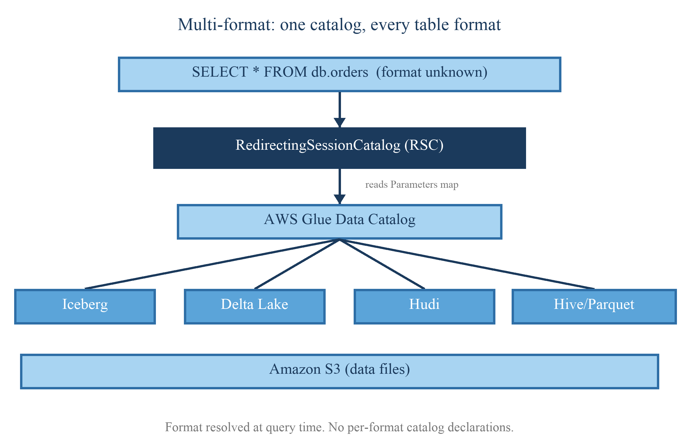
The following diagram shows how a single query flows through the RedirectingSessionCatalog to the correct format handler.
RedirectingSessionCatalog routing a query to Iceberg, Delta Lake, Hudi, and Hive handlers through AWS Glue

Figure 1: Multi-format routing. A single query enters the RedirectingSessionCatalog, which calls the AWS Glue Data Catalog to read each table’s format, then routes the table to the matching format-specific handler (Iceberg, Delta Lake, Hudi, or Hive) so results return through one catalog

As the diagram illustrates, the query enters through spark_catalog (the RSC). The RSC reads each table’s format from the AWS Glue Data Catalog and routes the operation to the matching engine: Iceberg, Delta Lake, Hudi, or Hive/Parquet. The four format handlers read the underlying data files from Amazon Simple Storage Service (Amazon S3). The caller issues one query with no format-specific catalog prefixes.

Multi-catalog: Cross-account access

When production data lives in a separate AWS account from your analytics compute, you can declare a named RSC catalog that points at that account’s AWS Glue Data Catalog. RSC resolves tables in the remote account the same way it resolves local tables, so a single query can join across accounts without copying data.

Previously, cross-account table resolution worked only for Iceberg (V2 catalog). Hive, Delta Lake, and Hudi tables in another account required manual Lake Formation and AWS RAM configuration rather than catalog-level resolution. With Amazon EMR 8.1.0, you declare a named RSC catalog for the remote account:

Configuration:

# Declare a named catalog pointing at the remote account's Glue catalog.
# "prod" is any name you choose for this catalog.
spark.sql.catalog.prod = org.apache.spark.sql.connector.catalog.\
redirecting.RedirectingSessionCatalog

# Tell it to use Glue as the metastore backend.
spark.sql.catalog.prod.metastore.type = glue

# Point it at the remote account's Glue catalog ID.
spark.sql.catalog.prod.metastore.hadoop.hive.metastore.glue.catalogid = 111122223333

Query:

-- Join local and remote tables directly. No data copy.
SELECT o.order_id, f.status
FROM spark_catalog.analytics.orders o -- local Iceberg table
JOIN prod.salesdb.fulfillment f -- remote Hudi table (account 111122223333)
ON o.order_id = f.order_id;

Each named RSC instance creates its own V1 metastore delegate and registers it with the global SessionCatalog, removing the singleton limitation.

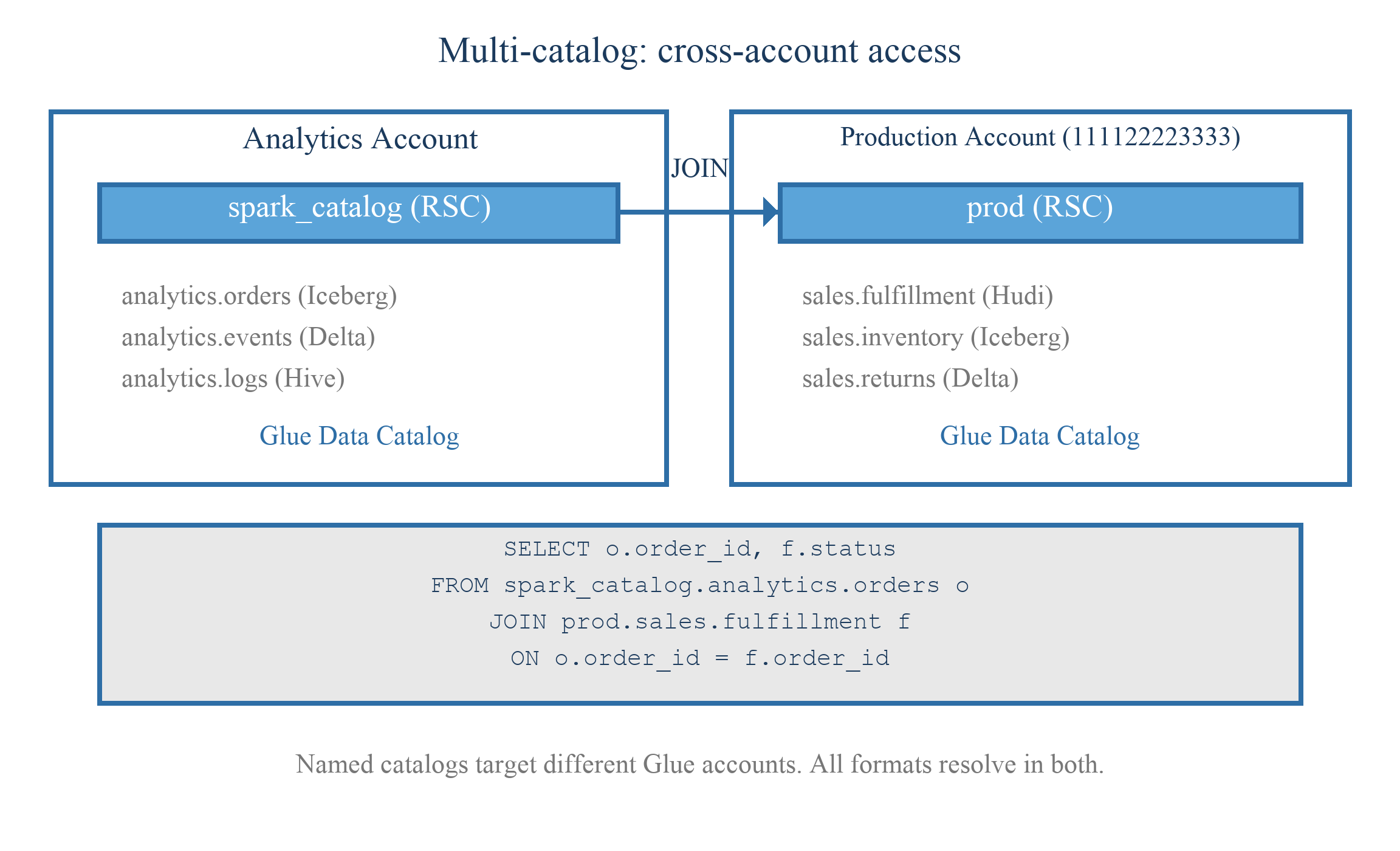
The following diagram shows how a single query joins tables across two AWS accounts through named catalogs.
A query joining a local table and a remote table across two AWS accounts through named catalogs

Figure 2: Cross-account access. A query in the local account references a named RSC catalog that points at a second account’s AWS Glue Data Catalog, so the local and remote tables join in one query without copying data between accounts

As the diagram illustrates, the analytics account uses spark_catalog (the RSC) for its local Glue Data Catalog, while a named catalog (prod) points at the production account’s Glue Data Catalog. The query joins a local table to a remote table in a single statement, shown by the JOIN between the two accounts. Each account keeps its own Glue Data Catalog, and no data is copied between them.

Auto-wiring

The preceding multi-catalog setup requires you to pre-declare each remote catalog in spark.sql.catalog.* properties. Auto-wiring in Amazon EMR 8.1.0 removes this requirement at two levels.

Before Amazon EMR 8.1.0, you declared the resolver, a handler per format, and each handler’s delegate class explicitly:

# Declare the resolver, a per-format handler, and each handler's delegate catalog
spark.sql.catalog.spark_catalog.table-format-resolver = \
com.amazonaws.glue.catalog.redirecting.GlueTableFormatResolver
spark.sql.catalog.spark_catalog.handler.iceberg = \
org.apache.spark.sql.connector.catalog.redirecting.DefaultTableFormatCatalogHandler
spark.sql.catalog.spark_catalog.handler.delta = \
org.apache.spark.sql.connector.catalog.redirecting.DefaultTableFormatCatalogHandler
spark.sql.catalog.spark_catalog.handler.hudi = \
org.apache.spark.sql.connector.catalog.redirecting.DefaultTableFormatCatalogHandler
spark.sql.catalog.spark_catalog.iceberg.delegate-class = org.apache.iceberg.spark.SparkCatalog
spark.sql.catalog.spark_catalog.iceberg.catalog-impl = org.apache.iceberg.aws.glue.GlueCatalog
spark.sql.catalog.spark_catalog.delta.delegate-class = \
org.apache.spark.sql.delta.catalog.DeltaCatalog
spark.sql.catalog.spark_catalog.hudi.delegate-class = \
org.apache.spark.sql.hudi.catalog.HoodieCatalog

# Manually declare every remote catalog you might query
spark.sql.catalog.prod = ...RedirectingSessionCatalog
spark.sql.catalog.prod.metastore.type = glue
spark.sql.catalog.prod.metastore.hadoop.hive.metastore.glue.catalogid = 111122223333
spark.sql.catalog.staging = ...RedirectingSessionCatalog
spark.sql.catalog.staging.metastore.type = glue
spark.sql.catalog.staging.metastore.hadoop.hive.metastore.glue.catalogid = 444455556666

Auto-wiring reduces this to:

Configuration:

# Set the default catalog. EMR auto-registers Iceberg, Delta, Hudi handlers.
# No handler.* properties needed.
spark.sql.catalog.spark_catalog = org.apache.spark.sql.connector.catalog.\
redirecting.RedirectingSessionCatalog

# Enable catalog discovery. The resolver inspects the connection type and
# registers the catalog at query time, with no upfront spark.sql.catalog.* config.
spark.sql.catalogResolver = com.amazonaws.glue.catalog.\
redirecting.GlueCatalogResolver

# Optional. Falls back to the SDK default region chain. Set this to query Glue catalogs in a specific region.
spark.sql.catalogResolver.region = us-east-1

Query:

-- Reference a remote catalog by its account ID. No prior declaration exists.
-- EMR calls Glue GetCatalog, determines the type, registers it on the spot.
SELECT o.order_id, f.status
FROM spark_catalog.analytics.orders o
JOIN `111122223333`.sales.fulfillment f
ON o.order_id = f.order_id;

The AWS Glue Data Catalog resolver is opt-in. When enabled, Amazon EMR issues an AWS Glue GetCatalog API call each time a query references a catalog that hasn’t been registered. This isn’t enabled by default to avoid unintended API calls for catalog names that don’t exist.

At the handler level, setting the default catalog to RedirectingSessionCatalog is enough. Amazon EMR fills in the Iceberg, Delta, and Hudi handlers automatically, so you don’t need to write handler.* properties.

At the catalog level, when you enable the Glue catalog resolver, Amazon EMR discovers new catalogs on demand. The first time a query references an undeclared catalog, Amazon EMR calls the AWS Glue GetCatalog API, inspects the connection type, and registers the catalog at query time.

Dynamic discovery is functional in Amazon EMR 8.1.0 for three catalog types. For standard cross-account AWS Glue catalogs, the resolver registers a redirecting catalog and multi-format routing applies. For Amazon S3 Tables, a capability of Amazon S3, the resolver reads the federated AWS Glue metadata and routes through Iceberg for both reads and writes. It also supports Amazon Redshift Managed Storage.

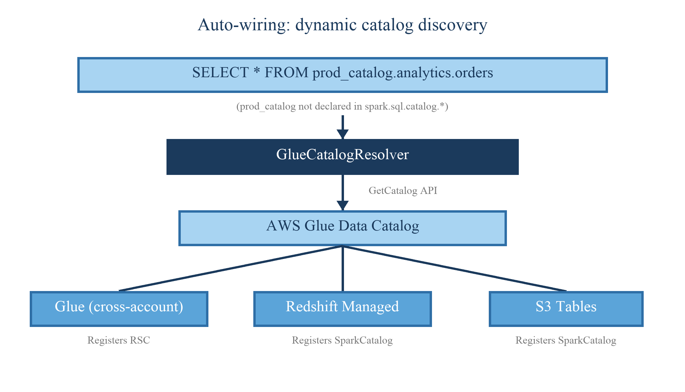
The following diagram shows how the GlueCatalogResolver discovers and registers a catalog the first time a query references it.
GlueCatalogResolver registering an undeclared catalog at query time through the AWS Glue GetCatalog API

Figure 3: Auto-wiring. When a query references an undeclared catalog, the Glue catalog resolver calls the AWS Glue GetCatalog API, inspects the connection type, and registers the catalog at query time, so no upfront catalog configuration is required

As the diagram illustrates, a query references a catalog that has not been declared, which raises a catalog-not-found condition. The GlueCatalogResolver intercepts it and calls the AWS Glue Data Catalog through the GetCatalog API. Based on the connection type, the resolver registers the appropriate catalog: a redirecting catalog for a cross-account AWS Glue Data Catalog, a push-down catalog for Redshift Managed Storage, or a Spark catalog for Amazon S3 Tables. Registration happens at query time, with no upfront configuration.

Quick start

Follow these steps to enable multi-catalog support on an existing Amazon EMR 8.1.0 application:

1. Set spark_catalog to the RedirectingSessionCatalog:

spark.sql.catalog.spark_catalog = org.apache.spark.sql.connector.catalog.\
redirecting.RedirectingSessionCatalog

Note: If using Delta Lake or Hudi, also add open table format (OTF) session extensions. Hudi additionally requires KryoSerializer.

Note: To query a different AWS account, add a named catalog pointing to that account’s AWS Glue Data Catalog.

2. (Optional) Enable the Glue catalog resolver:

spark.sql.catalogResolver = com.amazonaws.glue.catalog.\
redirecting.GlueCatalogResolver

Step 1 is all you need for Iceberg-only multi-format queries. The notes call out additional configuration for Delta Lake, Hudi, or cross-account scenarios. Step 2 removes the need to pre-declare catalogs by resolving them at query time.

Try it yourself

The following walkthrough creates four tables (one per format), runs a cross-format join, and extends to a cross-account query. The accompanying sample scripts handle resource creation, job submission, and cleanup. The accompanying code is in the aws-emr-utilities repository.

Prerequisites

  • An AWS account with permissions for Amazon EMR Serverless, AWS Glue Data Catalog, and Amazon S3.
  • An Amazon EMR Serverless application running release emr-spark-8.1.0 (Spark). The multi-catalog features also work on Amazon EMR on EC2 and Amazon EMR on EKS.
  • An Amazon EMR Serverless job execution role scoped to the specific AWS Glue databases and S3 prefixes.
  • An S3 bucket for scripts and output (this post uses s3://amzn-s3-demo-bucket/multicatalog/).
  • (For cross-account) A producer account with Lake Formation grants, AWS Glue resource policy, Amazon S3 bucket policy, and AWS Key Management Service (AWS KMS) key policy configured.

Step-by-step implementation

Step 1: Clone the repository and configure

git clone https://github.com/aws-samples/aws-emr-utilities.git
cd aws-emr-utilities/examples/emr-multi-catalog
cp env.template .env
# Edit .env with your application ID, role ARN, bucket, and region

The repository contains two phases: single-account multi-format and cross-account. The .env file stores resource identifiers referenced by all scripts.

Step 2: Bootstrap the environment

./scripts/bootstrap.sh

This script creates the AWS Glue database, uploads PySpark scripts to S3, and verifies that your Amazon EMR Serverless application is in CREATED state. Note the application ID from the output if you have not set it in .env.

Step 3: Create tables across four formats

./scripts/run_demo.sh --phase setup

The setup phase submits a PySpark job that creates one table per format (Iceberg, Delta Lake, Hudi, Hive/Parquet) in a single AWS Glue database with a shared id/val schema. Each CREATE TABLE uses a different USING clause but all go through the same spark_catalog. RSC routes each to the correct engine.

The job configuration includes the RedirectingSessionCatalog, OTF session extensions for Delta and Hudi, and KryoSerializer for Hudi. If your workload is Iceberg-only, you can omit the extensions and serializer.

Step 4: Run the cross-format join

./scripts/run_demo.sh --phase query

This submits a query that references four tables by database.table only, with no format prefix. The query joins all four through a single catalog with no format-specific configuration:

SELECT i.id, i.val AS iceberg, d.val AS delta, h.val AS hudi, p.val AS hive
FROM salesdb.orders_iceberg i
JOIN salesdb.returns_delta d ON i.id = d.id
JOIN salesdb.shipments_hudi h ON i.id = h.id
JOIN salesdb.products_hive p ON i.id = p.id;

Expected output:

+---+---------+-------+-------+------+
| id| iceberg | delta | hudi | hive |
+---+---------+-------+-------+------+
| 1| ice-1 | dl-1 | hu-1 | hv-1 |
| 2| ice-2 | dl-2 | hu-2 | hv-2 |
| 3| ice-3 | dl-3 | hu-3 | hv-3 |
+---+---------+-------+-------+------+

Each column came from a different table format, joined in one query with no format-specific catalog configuration.

Step 5: (Optional) Extend to cross-account

Cross-account access requires grants from the account that owns the data. Run one bootstrap in each account:

# In the consumer account (where EMR runs):
./scripts/bootstrap_consumer.sh --region us-east-1 \
--producer-account 111122223333

# In the producer account (which owns the data):
./scripts/bootstrap_producer.sh \
--consumer-role <ROLE_ARN from previous step>

Then, back in the consumer account, run the cross-account phase:

./scripts/run_demo.sh --phase xacct-autowire \
--producer-account 111122223333 --producer-table fulfillment

The result joins the producer account’s table to a local Iceberg table in a single query, with no data copy.

For the full cross-account policy setup (Lake Formation grants, AWS Glue resource policy, S3 bucket policy, and AWS KMS key policy), see the Cross-account setup section.

Tip: Add –dry-run to either bootstrap script to preview every action it would take (buckets, roles, policies, applications) without creating anything.

Clean up

To avoid ongoing charges, run the clean-up script or follow the steps in the repository README:

./scripts/cleanup.sh

This removes S3 data, AWS Glue databases and tables, Lake Formation permissions, and the Amazon EMR Serverless application.

Cross-account setup

Cross-account access requires configuration across four services. The following example shows the AWS Glue resource policy. The accompanying bootstrap_producer.sh script configures all four, so you don’t need to author each policy by hand.

1. AWS Lake Formation: Grant permissions on the database and tables to the consumer principal.

2. AWS Glue resource policy: Allow cross-account access to catalog metadata.

3. Amazon S3 bucket policy: Allow access to the underlying data files.

4. AWS KMS key policy: Use a customer managed key (the aws/glue managed key doesn’t support cross-account grants).

Example: AWS Glue resource policy

{ "Version": "2012-10-17", "Statement": [{
"Effect": "Allow",
"Principal": {"AWS": "arn:aws:iam::444455556666:role/EMRExecutionRole"},
"Action": ["glue:GetCatalog","glue:GetDatabase","glue:GetDatabases",
"glue:GetTable","glue:GetTables","glue:GetPartition","glue:GetPartitions"],
"Resource": ["arn:aws:glue:us-east-1:111122223333:catalog",
"arn:aws:glue:us-east-1:111122223333:database/*",
"arn:aws:glue:us-east-1:111122223333:table/*/*"]
}]}

Choosing the right configuration

Your situation What to set
Lake has Iceberg, Delta, and Hudi tables spark.sql.catalog.spark_catalog = RedirectingSessionCatalog (Delta and Hudi require additional spark.sql.extensions. See Quick start)
Analytics in one account, data in another spark.sql.catalog.<name> pointing at the remote Glue account (see Multi-catalog section)
Many accounts, want zero upfront config spark.sql.catalogResolver = GlueCatalogResolver
All of the above All three. They compose.

Note: Multi-catalog is query-time resolution. It doesn’t copy data between accounts, replicate tables, or grant access. Cross-account reads still require Lake Formation grants, AWS Glue resource policies, Amazon S3 bucket policies, and (if encrypted) AWS KMS key policies.

Conclusion

In this post, we configured the RedirectingSessionCatalog as the default Spark catalog on Amazon EMR 8.1.0. With a single configuration property, the RSC resolved Iceberg, Delta Lake, Hudi, and Hive tables through one catalog without format-specific prefixes. We then declared a named catalog to join tables across two AWS accounts, and enabled the GlueCatalogResolver to discover remote catalogs at query time without pre-declared spark.sql.catalog.* properties.

Multi-catalog support is available on Amazon EMR 8.1.0 across all deployment models: Amazon EMR Serverless, Amazon EMR on EC2, and Amazon EMR on EKS. To reproduce the walkthrough, clone the aws-samples/aws-emr-utilities repository and follow the steps in the Quick start section.

To learn more and get started, explore the following resources:


About the authors

Suthan Phillips

Suthan Phillips

Suthan is a Senior Specialist Solutions Architect at AWS, helping customers design and optimize scalable, high-performance data platforms that turn data into business insights. He brings expertise in system architecture, performance tuning, and security best practices across the full data stack, from ingestion and processing to analytics and visualization. Outside of work, Suthan enjoys swimming, hiking, and exploring the Pacific Northwest.

Manjeet Chayel

Manjeet Chayel

Manjeet serves as Big Data Manager, Worldwide Specialist Solutions Architects at AWS, where he leads a global team of specialist architects driving customer-facing engagements across Amazon EMR, AWS Glue, and the broader Big Data Analytics portfolio. With over 15 years at Amazon, he brings deep expertise in big data processing and building experiences that operate reliably at massive scale. He combines work with customers architecting their analytics platforms with a focus on scaling and developing the next generation of technical leaders across AWS.

[$] Python’s two modules for random numbers

Post Syndicated from jake original https://lwn.net/Articles/1097468/

Python’s random
and secrets
modules both include utilities for obtaining random values, but only one of them is suitable for generating passwords and security tokens.
For much of Python’s history, random was used for passwords and tokens anyway, despite documentation that called it unsuitable for cryptography.
In 2015, Python’s core team debated whether to fix that misuse by making random secure by default.
Instead, in 2016, Python 3.6 added a second module: secrets. The
random module is still misused at times, so it is instructive
to look into how the random-number modules should be used.

Securing Agent-to-Agent Communication: The Next Identity Frontier

Post Syndicated from Umair Mazhar original https://www.rapid7.com/blog/post/ai-securing-agent-to-agent-communication-next-identity-frontier

As organizations deploy autonomous AI agents, security teams face a significant shift as non-human non-human entities making decisions, invoking tools, and delegating tasks to other agents without human intervention. Security architectures built around human users, static APIs, and distinct endpoints break down when AI agents dynamically collaborate across an environment. 

As these interactions become more common, securing agent-to-agent communication without blocking adoption will require security leaders to treat autonomous agents as first-class identities, with their own permissions, behaviors, and activity to monitor.

The operational reality: A new attack surface

Consider a standard enterprise scenario where a primary agent delegates a task to a secondary agent, which then queries a production database through the Model Context Protocol and forwards a summary to external infrastructure. Traditional controls may struggle to capture the complete interaction, leaving security teams without visibility into intent, delegation chains, and scope of authority and introducing five security challenges that deserve particular attention:

  1. Identity and delegation chaining requires verifying an agent’s identity while ensuring its delegated authority never exceeds the permissions of the initiating user.

  2. Behavioral drift creates detection blind spots because when autonomous agents adapt execution paths dynamically, distinguishing normal operational variance from compromise or prompt injection becomes extremely difficult.

  3. Tool and protocol abuse allows agents to invoke APIs and tools autonomously, meaning that without strict guardrails, an agent quickly becomes an unwitting vector for data exfiltration or unauthorized execution.

  4. Cascading access can create systemic risk when a compromised high-privilege agent influences secondary agents and expands access across interconnected enterprise systems.

  5. Observability gaps arise when fragmented API logs cannot reconstruct multi-agent decision paths or explain why a particular action took place.

How agent activity fits existing security operations

Agent-to-agent communication can be treated as an extension of the security telemetry teams already collect across users, endpoints, cloud workloads, and applications. Bringing agent identities, delegation paths, tool invocations, and data access into the same investigation model allows existing detection engineering and behavioral analytics practices to evolve alongside agentic workloads.

For example, when a user initiates an action through a primary agent that delegates work to a secondary agent, the resulting identity chain and tool activity can be correlated with authentication events, endpoint activity, and network logs. This gives analysts a more complete investigation timeline, from the initiating user through each agent and tool involved.

Entity-based context expands the security model beyond users and devices to include AI agents as entities, allowing analysts to trace activity from the initiating user through sub-agents and tools.

Behavioral analytics can similarly extend from User Behavior Analytics toward Agent Behavior Analytics. By establishing baselines for how agents normally behave, detection engines can identify anomalies such as unexpected inter-agent communication, sudden privilege escalation, or unusually high-volume transfers.

Managed detection and response can incorporate agentic telemetry alongside the users, endpoints, and cloud workloads already monitored. Investigation workflows can then account for agent relationships, delegated actions, and tool invocations as part of the wider security picture.

Separation of duties remains important at the execution layer, where authorization gateways can enforce preventative policies while security operations maintain the broader visibility and behavioral detection needed when controls are misconfigured or bypassed.

How security teams can prepare for agent-to-agent communication

Security teams can begin preparing for autonomous agent workloads by extending familiar identity, telemetry, and least-privilege practices into agentic environments:

  1. Audit custom and third-party AI agents operating across the environment, including their active communication paths and tool access levels.

  2. Enforce least-privilege delegation by using temporary, task-scoped credentials tied to specific job definitions rather than persistent administrative permissions.

  3. Standardize telemetry requirements so teams capture structured logs for inter-agent delegation, tool invocations, and dataset access.

  4. Feed agent event streams into the Rapid7 platform to support behavioral detections for identity anomalies, authorization drift, and high-frequency communication between previously unlinked agents.

Build agent security into the SOC before autonomy scales

Agent-to-agent security is still evolving, but security teams can begin preparing now by extending principles they already understand across identity, access, visibility, and detection. Strong identity, least privilege, behavioral analytics, continuous monitoring, and detection and response provide a practical foundation for governing autonomous agents as they interact with systems and with one another.

As agent adoption grows, organizations will also need to make these interactions visible as part of normal security operations. For Rapid7 customers, agent activity could increasingly become another source of security telemetry and behavioral context, allowing analysts to follow the full chain from the initiating identity through delegated agents, tool invocations, and data movement.

The practical objective is to enable trusted agent collaboration while keeping each identity, delegation, action, and data movement observable, governed, and accountable. Organizations that begin building that visibility now will be better positioned to adopt autonomous agents without allowing their speed and flexibility to outpace the controls designed to protect the business.

[$] Last rites for Gentoo’s Chromium package

Post Syndicated from jzb original https://lwn.net/Articles/1097760/

Chromium, the open-source
upstream project for Google’s Chrome web browser, is the browser of choice for
many Linux users. It has also gained a reputation as being difficult for Linux distributions to
package and build
: Chromium has a complex build system, the project bundles
many of its dependencies, and it has frequent releases. All of that, plus user
complaints, has led the maintainers of the Gentoo Chromium
package
to give up on trying to maintain the package.

OpenSSH 10.6 released

Post Syndicated from jzb original https://lwn.net/Articles/1098980/

Version 10.6 of OpenSSH
has been released. The announcement notes that the OpenSSH team has been
receiving a large number of AI-assisted security bug reports. “We very much
welcome these reports, especially when combined with human triage, analysis,
test-cases and particularly when accompanied by proposed fixes
“. As a
result, the project expects to be making more frequent releases to get updates
to users more quickly rather than batching the bug fixes until the next planned
release.

Notable changes in this release include enabling the hybrid post-quantum
ssh-mldsa44-ed25519 signature algorithm, addition of a -p option for sftp‘s lmkdir/mkdir commands, as well
as disabling the LZ77 dictionary coder in ssh and sshd to mitigate side-channel
leaks (which will result in reduced effectiveness of the Compression
option). The scp -R option, which
allows copies between two remote hosts, is being deprecated due to security
risks; the option will be ignored in the future. See the announcement for full
details of all changes and bug fixes.

Security updates for Tuesday

Post Syndicated from jzb original https://lwn.net/Articles/1098979/

Security updates have been issued by AlmaLinux (gd, gimp, kernel, kernel-rt, libpcap, librabbitmq, mariadb-connector-c, osbuild-composer, ruby:2.5, and sudo), Debian (libmodule-cpants-analyse-perl, libpng1.6, libreoffice, roundcube, ruby-oauth2, and sabnzbdplus), Fedora (0install, alt-ergo, apron, brltty, chromium, coccinelle, cri-o1.36, emacs-common-tuareg, flocq, frama-c, freetennis, gappalib-coq, guestfs-tools, haxe, hevea, hivex, kernel, lem, libguestfs, libnbd, nbdkit, not-ocamlfind, ocaml, ocaml-afl-persistent, ocaml-alcotest, ocaml-astring, ocaml-atd, ocaml-augeas, ocaml-b0, ocaml-base, ocaml-base64, ocaml-benchmark, ocaml-bin-prot, ocaml-biniou, ocaml-bisect-ppx, ocaml-bos, ocaml-cairo, ocaml-calendar, ocaml-camlbz2, ocaml-camlidl, ocaml-camlimages, ocaml-camlp-streams, ocaml-camlp5, ocaml-camlp5-buildscripts, ocaml-camlpdf, ocaml-camomile, ocaml-capitalization, ocaml-cinaps, ocaml-cmdliner, ocaml-compiler-libs-janestreet, ocaml-cpdf, ocaml-cppo, ocaml-crowbar, ocaml-cryptokit, ocaml-csexp, ocaml-csv, ocaml-ctypes, ocaml-cudf, ocaml-curl, ocaml-curses, ocaml-dbus, ocaml-domain-name, ocaml-dose3, ocaml-dune, ocaml-easy-format, ocaml-expat, ocaml-extlib, ocaml-facile, ocaml-fieldslib, ocaml-fileutils, ocaml-findlib, ocaml-fmt, ocaml-fpath, ocaml-gen, ocaml-gettext, ocaml-graphics, ocaml-gsl, ocaml-integers, ocaml-intrinsics-kernel, ocaml-jane-street-headers, ocaml-jsonm, ocaml-jst-config, ocaml-lablgl, ocaml-lablgtk, ocaml-lablgtk3, ocaml-labltk, ocaml-lacaml, ocaml-lambda-term, ocaml-libvirt, ocaml-linenoise, ocaml-logs, ocaml-luv, ocaml-lwt, ocaml-mccs, ocaml-mdx, ocaml-menhir, ocaml-merlin, ocaml-mew, ocaml-mew-vi, ocaml-mlgmpidl, ocaml-mlmpfr, ocaml-monolith, ocaml-mtime, ocaml-mysql, ocaml-num, ocaml-obuild, ocaml-ocamlbuild, ocaml-ocamlgraph, ocaml-ocamlnet, ocaml-ocp-indent, ocaml-ocplib-endian, ocaml-ocplib-simplex, ocaml-omake, ocaml-omd, ocaml-opam-0install-cudf, ocaml-opam-file-format, ocaml-ounit, ocaml-parmap, ocaml-parsexp, ocaml-patch, ocaml-pcre2, ocaml-perl4caml, ocaml-postgresql, ocaml-pp, ocaml-pprint, ocaml-ppx-assert, ocaml-ppx-base, ocaml-ppx-bench, ocaml-ppx-bin-prot, ocaml-ppx-cold, ocaml-ppx-compare, ocaml-ppx-custom-printf, ocaml-ppx-derivers, ocaml-ppx-deriving, ocaml-ppx-deriving-yaml, ocaml-ppx-deriving-yojson, ocaml-ppx-enumerate, ocaml-ppx-expect, ocaml-ppx-fields-conv, ocaml-ppx-globalize, ocaml-ppx-hash, ocaml-ppx-here, ocaml-ppx-inline-test, ocaml-ppx-let, ocaml-ppx-optcomp, ocaml-ppx-sexp-conv, ocaml-ppx-stable-witness, ocaml-ppx-variants-conv, ocaml-ppxlib, ocaml-ppxlib-jane, ocaml-psmt2-frontend, ocaml-ptmap, ocaml-pyml, ocaml-qcheck, ocaml-qtest, ocaml-re, ocaml-react, ocaml-res, ocaml-result, ocaml-rresult, ocaml-SDL, ocaml-sedlex, ocaml-sexplib, ocaml-sexplib0, ocaml-sha, ocaml-spdx-licenses, ocaml-sqlite, ocaml-ssl, ocaml-stdcompat, ocaml-stdio, ocaml-stdlib-random, ocaml-store, ocaml-swhid-core, ocaml-testo, ocaml-time-now, ocaml-topkg, ocaml-trie, ocaml-unionfind, ocaml-uucd, ocaml-uucp, ocaml-uunf, ocaml-uuseg, ocaml-uutf, ocaml-variantslib, ocaml-version, ocaml-xml-light, ocaml-xmlm, ocaml-xmlrpc-light, ocaml-yaml, ocaml-yamlx, ocaml-yojson, ocaml-zarith, ocaml-zed, ocaml-zip, ocaml-zmq, ocamlify, ocamlmod, opam, perl-DBI, planets, plplot, prooftree, python3.12, rocq, rocq-stdlib, supermin, unison, utop, virt-top, virt-v2v, why3, xen, z3, and zenon), Oracle (bind, expat, gawk, gdb, ghostscript, gimp, gvfs, kernel, libpcap, libvirt, mod_auth_openidc, openssh, rsync, thunderbird, and webkit2gtk3), Red Hat (vim), Slackware (cups), SUSE (apache-sshd, binutils, cups, docker-stable, java-11-openjdk, libraw-devel, libX11, pcre2, perl-DBI, python-msgpack, python312, python313-tokenizers, rpcbind, rpm, rubygem-rails-html-sanitizer, squid, sssd, terraform-provider-susepubliccloud, valkey, and wpa_supplicant), and Ubuntu (aodh, watcher, edk2, libreoffice, libxmltok, linux, linux-aws, linux-aws-5.15, linux-aws-fips, linux-azure, linux-azure-5.15, linux-azure-fde-5.15, linux-azure-fips, linux-fips, linux-gke, linux-gkeop, linux-hwe-5.15, linux-ibm, linux-ibm-5.15, linux-intel-iot-realtime, linux-intel-iotg, linux-intel-iotg-5.15, linux-kvm, linux-lowlatency, linux-lowlatency-hwe-5.15, linux-oracle, linux-realtime, linux-xilinx-zynqmp, linux-azure-5.4, linux-azure-fde, linux-gcp, linux-gcp-fips, linux-gcp-5.15, linux-oracle-5.15, linux-raspi, rabbitmq-server, and unbound).

Possible Vulnerability in Apple’s Automatic Reboot

Post Syndicated from Bruce Schneier original https://www.schneier.com/blog/archives/2026/10/possible-vulnerability-in-apples-automatic-reboot.html

404Media is reporting (alternate link) that a cyber-weapons arms manufacturer is exploiting a vulnerability in iOS to bypass its automatic reboot security feature. This is the feature that automatically puts an iPhone into a more secure state if it hasn’t been used for 72 hours.

The new technology to get around inactivity reboot was developed by Magnet Forensics, the company behind GrayKey, a popular tool sold to law enforcement agencies that allows them to unlock and access data stored in iPhones and Android smartphones. Magnet has developed a new device called GrayKey Preserve and a feature for its regular GrayKey devices called Evidence Preservation Mode, according to the video.

“This is an absolute game changer for iOS forensics and a function that I wish we had years ago,” a Magnet employee says in the leaked video, specifically mentioning that the solution is targeted at the iPhone’s inactivity reboot feature and the data it makes unavailable. GrayKey Preserve and Evidence Preservation Mode are also designed to combat another iPhone feature that automatically deletes certain data ­- such as cached locations, and recently deleted photos and iMessages ­- after a certain number of days. “We’re gonna be able to preserve that data for an infinite amount of time.”

Presumably, now that Apple engineers know that this flaw exists they can find and fix it. AI turns out to be really good at this sort of thing.

Another news article.

Биляна Курташева: Смисълът на остаряването е да ни извади от клишетата на младостта

Post Syndicated from Роси Михова original https://www.toest.bg/bilyana-kurtasheva-smisulut-na-ostaryavaneto-e-da-ni-izvadi-ot-klishetata-na-mladostta/

Въпросите задават Сюзан Зонтаг и Роси Михова

Биляна Курташева: Смисълът на остаряването е да ни извади от клишетата на младостта

Американската писателка Сюзан Зонтаг (1933–2004), която е авторка и на емблематични есета в областта на литературната критика, философията и фотографията, е от онзи тип хора, които обожават да правят списъци. В своите дневници, публикувани посмъртно през 2012 г., тя разкрива почти агресивната си обсесия от подреждането на думи в колонки. Според психолозите това е нейната защитна поза „en garde“ срещу вселенския хаос – нейното хапче за облекчение в моменти на болка, самоконтрол в моменти на лудост и бистрота на ума в моменти на вдъхновение. Във втората част от тези дневници – „Когато съзнанието е впрегнато в плътта (1964–1980)“, писателката споделя:

Аз оценявам стойностното, аз придавам стойност, аз създавам стойност, аз дори гарантирам самото „съществуване“. Оттук идва и моята непреодолима потребност да правя списъци. Нещата (музиката на Бетовен, филмите, бизнес корпорациите) няма да съществуват, ако не заявя интереса си към тях, като поне запиша имената им.

Изброяванията, които Зонтаг прави в своите записки, са най-различни – поетични, медицински, изповедални, работни, философски. Нейният син Дейвид Риф ги определя като своеобразна „инвентаризация на душата“. Писателката е убедена, че човек се дефинира от това, което консумира и цени, и че личният вкус е нещо много повече от набор естетически и интелектуални предпочитания. И пояснява:

Ние притежаваме визуален вкус, но и вкус по отношение на хората, на емоциите, действията. Съществува вкус в морала, дори вкус в идеите.

Всички тези списъци обаче са създадени от думи. А Зонтаг настоява да гледаме на тях не като на символи и знаци за декодиране, а като на материални неща – всяка дума със свой звук, текстура, тежест, ритъм и физическо присъствие. Точно затова днес обсъждаме списъците на тази забележителна жена с една безспорна познавачка на теорията и практиката на думите – литературната критичка, редакторка и преподавателка Биляна Курташева*. 

Обичате ли да правите списъци?

Да, обичам. А още повече обичам жеста, с който задрасквам някоя задача в тях. Имам и нематериални, „ментални“ списъци, които живеят в главата ми, разнасям ги напред-назад, често с години.

Може би затова Умберто Еко казва, че „ние правим списъци, защото не искаме да умрем“.

Точно така. Списъкът често е мека форма на отлагане. А отлагайки, си казваме: „Има още време, още не съм на финалната черта…“ Затова мразя думата „дедлайн“ (английският е още по-брутален в сравнение с нашето „краен срок“). Като наближи поредният, просто изчаквам тихо да ме отмине. Разбира се, това не минава без душевни терзания, защото работя с текстове, бавя други хора… А и просроченият дедлайн те лишава от усещането за свършена работа. Така че може би най-тормозещият списък е този с крайни срокове в минало време.

Интересно е, че списъкът е едновременно древно, но и модерно, дори постмодерно занимание. Например първите писмени свидетелства на глинените плочки от Месопотамия са на практика счетоводни отчети и инвентарни списъци на домашни животни и стоки. Също редици от думи за обучение на начинаещите писари.

От друга страна, в литературата на XX век списъкът се превръща в жанр. Помислете за списъците на Гео Милев с неговите изведени до абсурд изреждания – в поемата „Септември“, но и преди това в незавършената поема „Ад“: „автомобили / със сто конски сили / мотоциклети / кеби / фиакри / карети…“ Гео прекарва няколко месеца в Лондон през 1914 г., шокът от движението в мегаполиса не го напуска и по-късно, през 20-те, се излива в поемата. Уловил е специфичния момент, когато четиритактовият двигател още се състезава с конете по улиците…

Впрочем моето първо влизане в правенето на литература през 90-те беше под знака на списък. Тогава с Елин Рахнев и Невена Дишлиева започнахме списанието „Аспирин Б“ (после „Витамин Б“), замислено в онези карнавални, луди времена като „списание за литература и блус“. В неговия първи брой излезе нашият „манифест“, оркестриран от Елин. Това беше именно списък, патетичен и ироничен едновременно:

Биляна Курташева: Смисълът на остаряването е да ни извади от клишетата на младостта
Личен архив

Аз и до днес се чувствам малко неловко – влязох в това посвещение само защото името ми започва с Б. Но продължавам да се самооблъщавам от този ред: „На Борхес и Биляна“. (Смее се.)

Да се насочим към Вашите лични списъци. Можете ли да изброите прилагателни имена, които намирате за особено интересни?

Прилагателните най-бързо се изчерпват и най-лесно се превръщат в кич. Голям майсторлък е да намериш нестандартно, различно прилагателно. Не само такова, което „пасва“, а и такова което „се сбива“ със съществителното, към което се отнася. Например (както Светлозар Игов е забелязал) Пенчо Славейков на едно място употребява фразата „импресионистичен кеф“. Вижте какъв челен сблъсък на епохи, на географии и манталитети…

Но за да не избягам от отговора, ще кажа, че обичам прилагателното „шантав“. Харесва ми чисто фонетично, даже бях изкушена да кажа „шашав“. Харесва ми и защото е по-стара дума, а в същото време е някак cool – съвременна, позитивна, по-скоро комплимент, отколкото обида.

Малко шантаво се получава това, защото в списъка от интересни прилагателни самата Зонтаг включва думата barmy, която в разговорния британски означава точно „шантав, луд“, но по някакъв весел и забавен начин. Кои съществителни имена харесвате?

Когато дъщеря ни Рая беше съвсем малка, измисляхме всякакви скоропоговорки и броилки. Оттогава ми е останала двойката „шибидах и маракуя“. „Шибидах“ по принцип не е моя дума, не ми се налага да я използвам и подозирам, че дълго време не съм знаела какво точно значи. Но ми е приятна. Може би защото не се случва често немска дума да звучи по този източен, екзотичен, ако щете – турско-персийски начин. Така е и с „маракуя“. Нямам особено отношение към плода, но в самите звуци има танц, песен, тяло, животни някакви. А комбинацията от двете думи е направо сюрреализъм в действие.

Има ли думи, които са Ви абсолютно безинтересни?

Тук бих казала „творец“. В годините на късния соц тази дума е била твърде експлоатирана. С нея се е злоупотребявало в речи и лозунги до степен на пълно обезсмисляне. През 90-те настъпи езикова революция и тогава точно тези квазивъзвишени понятия започнаха да звучат нелепо и архаично, някак демоде, но не и винтидж. И днес, когато някой каже „творец“, за себе си вече знам къде стои и политически, и естетически, и всякак.

Като оставим настрана думите, можете ли да изброите неща, които просто харесвате?

Харесвам списъците и правенето им. Харесвам планини – и на живо, и на картинка. Харесвам имената им. Ходили сме навремето с баща ми по задължителните български Стара планина, Рила, Пирин, Родопите, Витоша, също в Татрите. По-късно с Рая и Георги сме обикаляли из Алпите, включително Доломитите… Това е хубава върволица от имена. Както пее Висоцки, „по-хубави от планините са само планините, в които не си бил“.

И разбира се, харесвам (тази дума е някак недостатъчна) книги – печатни, но не само. Слушам доста книги, докато разхождам кучето Йори. Харесвам хартията във всички нейни разновидности. Заедно с това непрекъснато се налага да се боря с нея, защото домът ни има свойството да акумулира купища хартия – книги, списания, вестници, записки, подсещащи листчета. Все неща, които най-трудно се подреждат и разчистват.

Стигнахме до списъка с неща, които не харесвате…

Не понасям насилието – на първо, второ, трето и десетнайсето място. Това е, което, ако можех, бих изтрила от света и от човешката природа. Впрочем то е голям въпрос и по отношение на изкуството. Трябва ли да се описва и показва насилие? Някой би казал: „Трябва, за да се изобличава“, но друг би казал, че така то се и нормализира. Границата е много тънка. Сцените на насилие са най-сигурният начин да „стиснеш за гърлото“ читателя или зрителя, но често той е и най-евтиният.

С годините все повече мисля за границата, до която насилието следва да бъде визуализирано. И ми се струва – малко парадоксално, – че само най-виртуозните писатели и режисьори имат право да оголят агресията. Сещам се за романа „Позор“ (Disgrace) на Джон Кутси, безмилостен и все пак (може би) щадящ и героите си, и читателите. В кулминационната сцена тишината в съседната стая се чува по-страшна от писък.

Казвам тези неща със съзнанието за вътрешно противоречие, защото като човек от 90-те съм почитател на Тарантино. При него стратегията е друга – смесване на бруталност и ирония на най-различни равнища. За мен си остава класическа началната сцена на „Глутница кучета“, където бандитите, които след малко ще направят въоръжен грабеж на банка, водят философски и социално ангажиран спор трябва ли да се дава бакшиш на сервитьорките…

И тук ще се изкуша да кажа нещо за многообсъжданата „Одисея“ на Нолан и защо съм от феновете ѝ. С всички ресурси на блокбастъра той би могъл да удави зрителя в кървища. С напредването на филма осъзнах, че за мен решаващ ще е начинът, по който той ще ни представи падането на Троя. То се случи относително късно, когато зрителите (поне аз) вече дори не го очакваха. А това е пример за фина работа с ритъма на разказа. В крайна сметка падането на града беше съкрушаващо, жестоко, но по един обран, пестелив начин, който те оставя да го доработиш в главата си. Не бяха показани масовите изнасилвания, убийства, обезглавявания – тоест показаха ни ги, без да ни ги показват. И това е важно стилистично и смислово решение.

Вижте какво пише Зонтаг в списъка си с новогодишни обещания: „Искам да се помоля, а не да си обещавам. Молитвата ми ще бъде за храброст. Не просто да събера смелост да бъда лоша писателка, трябва да се престраша да бъда наистина нещастна. Отчаяна. И да не се спасявам, заобикаляйки отчаянието си. Отказвайки да бъда толкова нещастна, колкото всъщност съм, аз се лишавам от теми. Нямам за какво да пиша.“

Зонтаг страда от комплекса на есеиста спрямо романиста. Тя е гениална есеистка, но иска на всяка цена да пише романи, може би оттам и част от самобичуването. Цитатът е силен и категоричен. Аз обаче бих искала да си обещая да не бъда чак толкова категорична. Защото, така както съм колеблива, флуидна, има моменти, в които съм склонна към прекалена твърдост. То е вид самовъзпаляване – човек взема засилка по дадена тема и вече не може да се спре.

Мисля си, че мъжете дори не подозират колко гневна може да бъде една жена на средна възраст. Гневът е категория, която по принцип техният пол отдавна е узурпирал. Това е залегнало в основата на нашия канон и култура: „Музо, възпей оня гибелен гняв на Ахила, сина Пелеев…“

Но ми се струва, че има доста гибелен гняв, натрупан и у жените, и то у жените на средна възраст. Той невинаги е насочен навън към някого или нещо. Жените сме абсолютни царици на самоизяждането. Но една жена, като стане на 50, някак изведнъж светът ѝ става ясен. Знам ли, може би се понижават онези хормони, които преди това са ни правили такива симпатичнички, щастливички, лековерни, податливи. И когато това опиянение, подобно на анестезия, се оттегли, настъпва една студена яснота. Променяме се и не съм сигурна, че хората около нас са готови за това. Дори начините, по които се нарича този период, са много показателни – немците го наричат Wechseljahre (години на промяна). В други езици се обозначава като пауза, а ние го наричаме „критическа възраст“. Бих казала, критическа и в смисъла на Кант, без той дори да подозира. Настъпва критика на чистия разум, който не е никак чист, и ние изведнъж проглеждаме за това.

Добре, в тези години на промяна кои са нещата, които възстановяват силите Ви?

Разхождането на куче, също четенето… Да си поговоря с дъщеря ни. Или да си помълча в някой ъгъл на денонощието, да си постоя сама. Изобщо страшно важно е човек от време на време да остава сам със себе си.

Както пише Зонтаг: „Да си сред хора и да си сам е като да вдишваш и издишваш, систола и диастола.“

Както винаги проницателна. Колкото повече напредваме в живота, толкова повече глаголът „дишам“ става важен. А по отношение на тази проницателност бих си позволила да подредя самата Зонтаг в един специален кратък списък: Хана Аренд, Сюзан Зонтаг, Джоун Дидиън – трите големи на американската проза, много различни, но и много сходни в умението да виждат зад кулисите на живота и света.

Дойде ред на списъка с препятствия и трудности. Кои са нещата, които ни спъват и дърпат назад?

Струва ми се, че в живота няма празни ходове. Ето ви пример – баща ми беше инженер, но истинската му страст бе чистата математика. И може би защото не беше успял да я реализира като своя професия, тази задача се прехвърли на мен. Така от детската градина до 11-ти клас в математическата гимназия ходех на математически школи, лагери и олимпиади. Решаването на задачи беше неизменна част от дневния ми режим. Докато накрая събрах кураж и му казах, че искам да следвам философия. В крайна сметка завърших българска филология, но поне научих, че математиката и литературата не са взаимно изключващи се вселени. Макар че на въпроса какво стана с еди-кой-си Ваш студент, един от големите математици отговаря: нямаше достатъчно талант и стана поет. А аз дори и поет не станах. (Смее се.)

Това чудесно се допълва с тезата на съпруга Ви, писателя Георги Господинов, че ние сме всичко, което ни се е случило, и всичко неслучило се също, че понякога неслучилото се е дори по-важно от случилото се.

Да, това е усещане и тема, които пронизват всичките му книги. В тях има нещо окуражаващо, но и нещо съкрушително. Човек никога не знае кога е от second best половината на сбъдването. (Смее се.) Но това е важна мотивация за писането, а и за четенето – да наваксваме откъм неслучило се.

Кажете кой е най-големият Ви интелектуален предразсъдък.

При нас, литераторите, предразсъдъците обикновено са на жанрова основа. Аз обичам фантастиката (от която много сериозни литератори също имат дистанция), но стоя далеч от фентъзито. Независимо от естествената близост между тези два жанра, имам предубеждение, дори високомерие към втория. Струва ми се твърде сладникав, повърхностен и клиширан, за да се нареди до сериозната научна фантастика. От друга страна, вече има много хибридни текстове, чиито автори демонстрират как може да се направи сглобка между фентъзи и фантастика – да речем, още Робърт Шекли и Робърт Зелазни го правят. Съществува дори такова литературно „животно“ като социално-политико-историческо фентъзи, каквото според мен е „Игра на тронове“.

В дневниците си Зонтаг дебатира и някои на пръв поглед странни въпроси. Например коя ръка предпочитате – лявата или дясната?

С удоволствие ще отговоря, защото у мен има лека обсесия на тема ръце. Първо, нямаме особена свобода да предпочитаме, защото природата залага коя ще е нашата по-силна ръка. Аз съм банален десничар. Заедно с това обаче по-силната ръка е по-бързо остаряващата. И при моите собствени ръце това много личи. Моята по-млада ръка е лявата. И затова по чисто естетически причини предпочитам нея.

Ще Ви цитирам дословно отговора на Зонтаг: „Дясната ръка е агресивната ръка, ръката, която мастурбира. Затова за предпочитане е лявата ръка. Тя може да бъде романтизирана, да бъде сантиментализирана.“

Да, виждам връзката. И при мен лявата ръка е някак по-изнежена, щадена, глезена.

Какво означава да си влюбен?

Хм, предполагам, че влюбеността е чувство в потенция. То е яйце, от което не знаеш какво ще се пръкне.

Напоследък по разни поводи и през разни четива попадам на думата „кайрос“. С нея древните гърци обозначават онзи кратък времеви прозорец, когато още не са се случили окончателни неща и всички избори и развръзки са възможни. Влюбването според мен попада точно в това мимолетие. Но пък ако се случи кайросът на влюбването да се сблъска с хроноса, тоест с вече установената темпоралност на подредения живот, това може да е катаклизъм. Не си го пожелавам.

Нека завършим този разговор по секси начин. Каква е тайната на добрия секс?

За мен сексът си остава мегапарадоксът на човечеството – едновременно най-голямото табу и най-натрапчиво нещо в света около нас. Най-наглото и най-уязвимото, с най-крехка граница между удоволствие и насилие. Днес всичко, за което можете да се сетите, трябва да е сексапилно – власт, дрехи, храна, дори краят на нашия разговор.

Но напук на масовата култура, рекламите, социалните мрежи и пр. сексът е по-скоро мозъчно, отколкото телесно преживяване. Или особено късо съединение между мозък и тяло. Впрочем неговата задължителност (на секса) е едно от най-големите клишета. И вероятно това е големият смисъл на зрялата възраст – да ни извади от клишетата на младостта.

Харесва ми дефиницията Ви за секса като късо съединение между тяло и мозък. Тази интерпретация донякъде тича в съседен коридор с отговора на Зонтаг: „Самоуважението. Това е тайната на добрия секс… Да можех само да чувствам към секса това, което чувствам към писането. Че съм проводникът, медиумът, инструментът на някаква сила отвъд мен самата.“

Красиво казано. А красивото има тази склонност да бъде и убедително.


* Биляна Курташева e доцент по теория и история на литературата в Нов български университет. Автор на книгите „По ръба на сравнението. Яворов и „Ролинг Стоунс“ и други не/възможни интертекстове“ и „Антологии и канон: антологийни модели на българската литература“. Била е главен редактор на сп. „Следва“, издание на НБУ за университетска култура, изкуства и хуманитаристика (2001–2020), и на експерименталното списание за литература и блус „Витамин Б“ (1996–1999).

How classroom challenges can change how students see computing

Post Syndicated from Dan Fisher original https://www.raspberrypi.org/blog/how-classroom-challenges-can-change-how-students-see-computing/

Computing education in England is in a stronger position than it was a decade ago. Increased access to technology, free learning resources for young people, and improved training for computing teachers has put us on a path to success. 

But the subject is also at an important inflection point. Young people are growing up in a world shaped by digital technologies like AI, yet not all young people get the same opportunities to discover how computing can be creative, collaborative, and relevant to their lives. This is reflected in the number of learners who choose to study it. In England, GCSE Computer Science entries fell by 4.7% in summer 2025 (93,980 to 89,610), and A level entries fell by 2.4% (19,475 to 19,010)*. 

Creating positive, accessible experiences early in a students’ education, and helping them to build confidence and see computing as something they can engage with, has never been more important.

For educators, computing is about much more than preparing learners for a single subject or qualification. Skills England’s 2025 assessment of priority skills up to 2030 estimates that demand for priority occupations will grow by 0.9 million, including 87,000 additional programmers and software development professionals**. These roles are identified as a priority across seven industry sectors, underlining the value of the broader skills students develop through computing: problem-solving, logical reasoning, creativity, and confidence.

That’s why initiatives such as the UK Bebras Challenge and the Raspberry Pi Foundation Coding Challenge matter. They give teachers ready-made, engaging ways to introduce computational thinking and coding without needing students to already see themselves as ‘computer scientists’. Low-barrier, fun, and practical, they help students experience the satisfaction of solving problems for themselves. As Mitchel Resnick, Professor of Learning Research at the MIT Media Lab, puts it: “They are not just learning to code, they are coding to learn.”***

The UK Bebras Challenge 2026

Over the past year, the UK Bebras Challenge (November 2025), and the Raspberry Pi Foundation Coding Challenge (March 2026), have reached hundreds of thousands of students across the UK.

Participation continues to grow. In 2025, 562,924 students took part in Bebras, up from 467,000 in 2024, contributing over 1 million hours of learning. The Coding Challenge also grew, with 85,389 students taking part in 2026, up from 83,096 in 2025.

To understand what this looks like at the grassroots level, we spoke to two teachers about why they run these challenges and what their students gain from taking part.

Johanna Watkins, Head of Computer Science at Highcliffe School, on the UK Bebras Challenge

Johanna Watkins, Head of Computer Science at Highcliffe School, on the UK Bebras Challenge

What made you decide to take part in the UK Bebras Challenge?

I was introduced to the Bebras Challenge during my teacher training, where my placement school was already taking part in the competition. Not only was it an affordable way to introduce students to the world of computational thinking, but I quickly realised how useful it was in identifying which students would be a good fit for GCSE Computer Science. Since my initial positive experience, I’ve ensured that all computer science students take part in the challenge, no matter which school I’ve worked in.

What makes Bebras different from other activities or competitions?

From an admin perspective, it is quick and easy to create accounts for a large number of students in one go. Once student data is downloaded from your MIS, importing the spreadsheets is incredibly simple. As a busy teacher, this saves me a lot of time.

For students, the accessibility of Bebras is a big selling point. Due to the on-screen reader, ability to add extra time for SEND students and differentiated challenges, everyone can access the competition. The interactive elements within the questions also make it engaging and enjoyable to work with.

How do students usually respond when they first encounter Bebras tasks?

Students can be easily influenced by their teachers. When introducing the Bebras Challenge every year, it’s important to clarify its purpose and the reason behind taking part. With a genuine motive explained, I find students are receptive to attempting something new. Every individual challenge is unique and colourful, operating a simple UI to jump between questions. Students are spurred on to get stuck into the puzzles on their first encounter, responding to the tasks with confidence.

What skills do you think students develop through Bebras?

The number one skill that students develop is their ability to problem-solve. When faced with tasks of varying difficulties, they are able to apply the key principles of abstraction and decomposition to tackle problems. If I’m with a GCSE or A Level class, it presents as the perfect opportunity to reinforce their theory knowledge, linking computational thinking concepts to the question in front of them.

Additionally, it can promote the hard skill of literacy. By having separate competitions for different year groups, students are reading texts that are of an appropriate level for their age bracket. And if you’re in a primary school, there’s the option to work in groups, allowing students to develop another soft skill of teamwork.

Can you share a specific example of a student benefiting from the challenge?

I’ve previously taught a Year 9 student with a reading age of 10, who was finding all aspects of school a challenge. Utilising the adaptive technology available to them in the Bebras Challenge, they were one of few in their class to achieve a Merit. This student was able to showcase their strong logical reasoning skills, without being hindered by their reading comprehension.

Consequently, they chose Computer Science as one of their GCSE options and wanted to pursue a career as a software developer. It also raised an interesting discussion point with the school, investigating various access arrangements to better support them. The Bebras Challenge has quite literally changed this student’s life.

What advice would you give to a teacher wanting to run the challenge in their school?

Just go for it! Given how renowned the competition is, my sixth form students have mentioned their results in university and apprenticeship applications. If students are needing evidence to back up their problem-solving abilities, or wanting to differentiate themselves from others with similar grades, the UK Bebras Challenge gives them an extra string to their bow.

As a teacher, just make sure you’re organised and prepare the accounts well in advance. Once the student accounts have all been created, using the helpful Coordinator Handbook as guidance, you can export their details and create login slips. Coupled with Bebras’ instructions presentation for in-class, it made for a smooth set-up and delivery. As the competition is straight after October half-term, it also allows teachers to ease their way back into school life. We always look forward to Bebras week at my school!

Isobel Culmer, Teacher of Computer Science at Barton Peveril School, on the Raspberry Pi Foundation Coding Challenge

Isobel Culmer, Teacher of Computer Science at Barton Peveril School, on the Raspberry Pi Foundation Coding Challenge

How did you first get involved with the Coding Challenge?

We are always looking for more competitions for students to participate in. We run a few competitions, but most are for the elite only. For example, we run the British Informatics Olympiad and British Algorithmic Olympiad but only about 20 of our 340 students can attempt either.

So when we heard about the Coding Challenge, it was exactly what we were looking for, a competition where everyone could take part and achieve good results. It’s always good to practise more coding skills, so this competition is ideal for us. This year was the first time we had the whole cohort take part, both Year 12 and Year 13.

How do students usually respond when they first encounter the Coding Challenge tasks?

The vast majority of students are excited about the Coding Challenge. They love competition!

The very first time they see them, it can be a bit overwhelming. There is a lot to do in a short time, which is why we get students to practise before the actual competition.

The emphasis of this challenge is firmly on coding compared to the computational thinking focus on the Bebras Challenge. Why is coding still an important skill to teach learners?

It has always been about problem solving. This is a skill that is still very much in demand, perhaps more so now. We are still teaching computational thinking when teaching them to code. There are many transferable skills from learning to code that are useful in most careers and industries. The need for resilience and attention to detail are vital skills for all.

Besides specific coding skills, what other skills do you think students develop through the Coding Challenge?

It develops resilience and many other skills such as following instructions precisely, which are important in life. Also time management and planning, students need to decide what to try and in what order if they want to maximise their score.

Can you share any examples of a student or group doing something in the Challenge that ignited their interest in computing?

Quite a few students will continue to work on the problems they encountered after the challenge has finished. They are determined to solve the problems! I hear many groups discussing techniques they used to solve the trickier problems which gives them the confidence to use those techniques in their classwork.

What advice would you give to a teacher wanting to run the Challenge in their school?

Do it! It is so easy to do. We run it in a normal lesson; it is in our schedule of lessons so all teachers do it the same week. From two weeks before the day we choose to set the challenge, we set homework to be practice questions.

The tricky part is making sure the students understand the interface, what code to copy in and how to test and run it, so the homework gives them a chance to do this. One teacher sets up the spreadsheet with all the student names to import to the very easy-to-use teacher admin website. It is then easy to download each class’s usernames and passwords.

Making computing accessible at scale

Across both challenges, one thing is clear: when barriers are lowered, more students take part and discover that computing is for them. Whether through short problem-solving tasks or coding challenges, these experiences build confidence, develop transferable skills, and help learners see themselves in computing.

For teachers, they also offer something equally important: practical, structured activities that can fit into the school year and work with whole classes or cohorts. In a landscape where the UK needs more young people to develop digital and computational skills, accessible challenges like these can help spark interest early, celebrate success, and give every learner a meaningful first step into computing.

How to get involved

To register your school for the next UK Bebras Challenge coming in November 2026, go to bebras.uk.

References

*https://www.gov.uk/government/statistics/provisional-entries-for-gcse-as-and-a-level-summer-2025-exam-series/provisional-entries-for-gcse-as-and-a-level-summer-2025-exam-series

**https://www.gov.uk/government/publications/assessment-of-priority-skills-to-2030/assessment-of-priority-skills-to-2030

***https://web.media.mit.edu/~mres/papers/L2CC2L-handout.pdf

The post How classroom challenges can change how students see computing appeared first on Raspberry Pi Foundation.

Smarter personalization: How property data helps us understand user price sensitivity

Post Syndicated from Grab Tech original https://engineering.grab.com/price-sensitivity-profiling-using-llm

Introduction

Existing systems estimate user price sensitivity primarily from spending behavior or demographic proxies. They do not systematically account for residential property values, which can indicate a user’s financial circumstances. This omission creates three limitations:

  1. Limited property insights: Existing profiles do not account for property values.
  2. One-dimensional profiles: Users with similar spending patterns but different living standards receive the same classification.
  3. Regional variation: Manual classification does not adapt well to differences between property markets.

This invention adds property data to user profiles to produce affluence segments that account for regional property markets. The invention remains unimplemented and is not deployed in any live market.

Background

Property values vary across buildings, neighborhoods, and regions. A useful classification method must account for these differences while processing property records in several formats. The same classification method could support other industries that use affluence segments.

Solution

A four-step method that combines public property data with clustering techniques to classify user affluence was created:

  1. Data collection and enrichment.
  2. Building-level property price estimation.
  3. Property tier classification.
  4. User mapping to affluence tiers.

The method combines external property data, large language model (LLM) enrichment, and cluster-based segmentation. The resulting profiles can inform personalized offers, targeted marketing, and operational planning.

Data gathering and processing

The system collects public property data from external sources. These records include transaction prices, building types, and related attributes in raw text formats. LLMs standardize the records and extract key attributes such as postcode, building address, transaction price, price per square meter, property size, and floor level. This stage produces a structured property-level dataset for analysis and modeling.

Building-level price estimation

Under the proposed method, transaction records for properties within the same building would be aggregated to calculate a weighted average sale price. The weighting would account for transaction recency and data volume, with the aim of reflecting recent market conditions.

When transaction data is limited, the method could apply rules based on comparable properties in the area. It could also evaluate LLM-assisted extraction of contextual signals from appropriately licensed external sources, such as real estate listings. Any LLM-derived signals would require validation against independent reference data before contributing to a property-value estimate.

The invention has not been implemented, deployed, or tested in a live market. Its model and version, validation methodology, error bounds, and operational safeguards remain subjects for future technical evaluation.

Property tier classification

A hierarchical clustering model groups buildings into affluence tiers based on their estimated resale values. The model accounts for regional differences and local market-value distributions across property types and locations. This stage assigns each building to an affluence tier.

User mapping to property tiers

The system maps would use appropriately aggregated geographic signals to associate users with broad property-market segments and assign a corresponding affluence classification.

Potential future applications

This invention presents a conceptual approach for exploring new ways to support personalization, advertising, and operational planning. It has not been implemented, deployed, or tested in a live market. Subject to technical validation and approval from Privacy, Legal, PR, and the relevant product owners, potential applications could include:

  • Personalization: Tailoring promotions, discounts, subscription plans, and recommendations for optional products and services.
  • Advertising: Supporting more relevant connections between advertising content, merchants, and broad audience segments, alongside tailored marketing campaigns.
  • Operational planning: Informing aggregated analysis used to plan and prioritize delivery and transport capacity.

Learnings and conclusion

This invention presents a conceptual approach that combines publicly available property data, LLM-assisted data structuring, building-level value estimation, hierarchical clustering, and contextual tier assignment. It demonstrates how regional property-market context could complement existing signals, while highlighting dependencies on data quality, model accuracy, geographic coverage, privacy, and fairness.

The approach shows potential applications in personalization, advertising, and operational planning, but these are illustrative, not demonstrated outcomes.

Join us

Grab is a leading superapp in Southeast Asia, operating across the deliveries, mobility, and digital financial services sectors. Serving over 900 cities in eight Southeast Asian countries: Cambodia, Indonesia, Malaysia, Myanmar, the Philippines, Singapore, Thailand, and Vietnam. Grab enables millions of people every day to order food or groceries, send packages, hail a ride or taxi, pay for online purchases or access services such as lending and insurance, all through a single app. We operate supermarkets in Malaysia under Jaya Grocer and Everrise, which enables us to bring the convenience of on-demand grocery delivery to more consumers in the country. As part of our financial services offerings, we also provide digital banking services through GXS Bank in Singapore and GXBank in Malaysia. Grab was founded in 2012 with the mission to drive Southeast Asia forward by creating economic empowerment for everyone. Grab strives to serve a triple bottom line. We aim to simultaneously deliver financial performance for our shareholders and have a positive social impact, which includes economic empowerment for millions of people in the region, while mitigating our environmental footprint.

Powered by technology and driven by heart, our mission is to drive Southeast Asia forward by creating economic empowerment for everyone. If this mission speaks to you, join our team today!

Materialize once, query anywhere: Introducing Iceberg materialized views in Amazon Redshift

Post Syndicated from Sudipta Bagchi original https://aws.amazon.com/blogs/big-data/materialize-once-query-anywhere-introducing-iceberg-materialized-views-in-amazon-redshift/

Amazon Redshift has progressively deepened its integration with Apache Iceberg. Earlier this year we launched Amazon Redshift RG, powered by AWS Graviton, with a purpose-built, integrated vectorized query engine designed from the ground up for data lakes. Instead of sending scans to a separate fleet, RG runs them natively on the cluster using vectorized Parquet scans, a smart-prefetch I/O subsystem, partition- and file-level pruning, improved bloom filters, and automatic Iceberg statistics collection through JIT Analyze for better query plans. Together, these deliver up to 2.4x faster Apache Iceberg queries than RA3, at 30 percent lower cost per vCPU and with no per-terabyte scan charges on data lake queries. On top of that performance foundation, you can write directly to Iceberg tables with full ACID alignment using INSERT, CTAS, UPDATE, DELETE, and MERGE. You can govern access with AWS Identity and Access Management (IAM) permissions through the external schema’s IAM role or with AWS Lake Formation for fine-grained, cross-engine control.

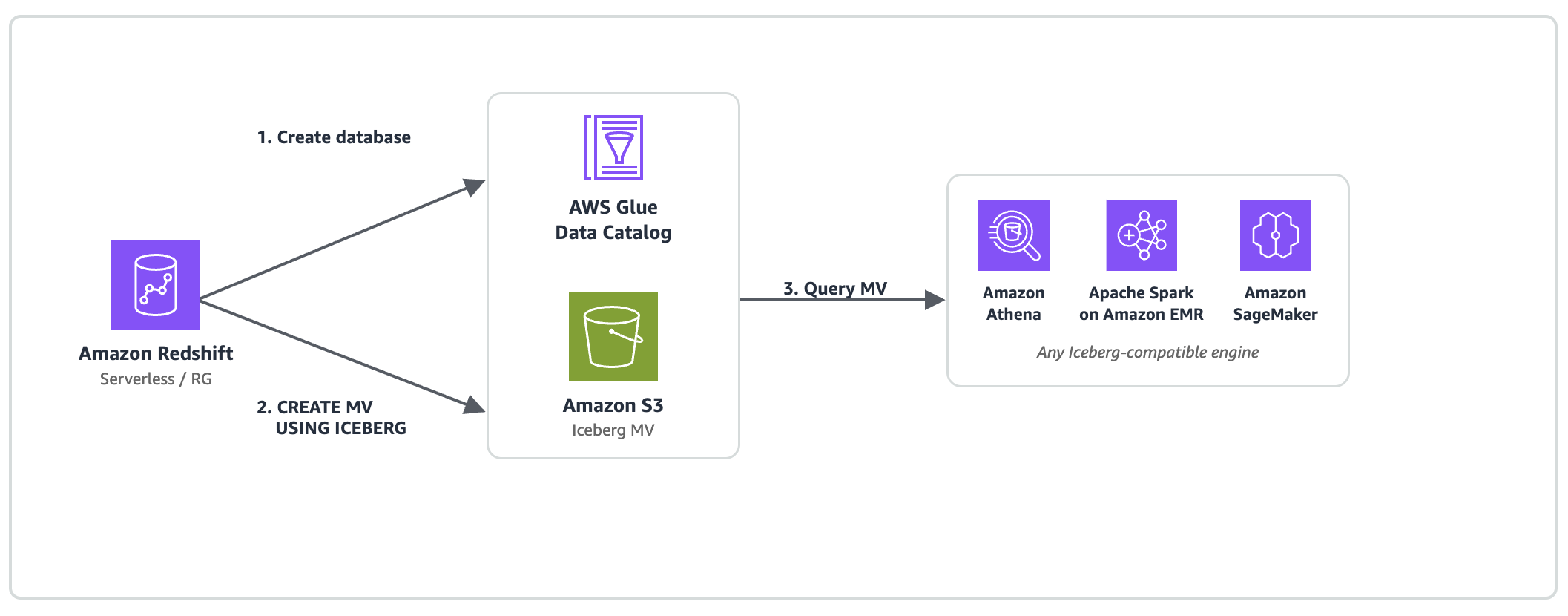
Amazon Redshift now also supports creating and refreshing Iceberg materialized views. A materialized view (MV) pre-computes expensive joins and aggregations once and stores the result as a standard Apache Iceberg table in Amazon Simple Storage Service (Amazon S3) or Amazon S3 Table Buckets, registered in the AWS Glue Data Catalog. You create one using familiar SQL (CREATE MATERIALIZED VIEW ... USING ICEBERG), and the result is instantly queryable by Iceberg-compatible engines, including Amazon Athena, Apache Spark on Amazon EMR, and AWS Glue. Amazon Redshift keeps it current with incremental refresh, and because the result is an ordinary Iceberg table in the AWS Glue Data Catalog, it is governed and discovered like any other catalog table.

Consider a team that runs its analytics on Amazon Redshift. Their transformations are already written in Amazon Redshift SQL, their staff know Amazon Redshift, and they’ve invested in its query engine. What they don’t have is a way to share their most expensive pre-computed results with the other engines in their organization, such as a data science group on Spark or an ad-hoc reporting team on Athena, without exporting copies or standing up a second transformation stack. The gap for this team is that they want interoperability and acceleration from the engine they already run.

Now they can create this materialized view in Amazon Redshift, in the SQL they already write, and Amazon Redshift stores the pre-computed result as an open Iceberg table. The Spark and Athena teams read that same result directly, without maintaining copies or separate pipelines. As new data lands, incremental refresh recomputes only what changed. The team gets a single, consistent source of truth for its most expensive queries that every engine shares. The Amazon Redshift team can run an end-to-end transformation pipeline in one engine, using materialized views as the building block between raw, cleaned, and serving layers without stitching multiple engines together stage by stage.

And you don’t need to choose between open and fast: for your most latency-sensitive dashboards, you can still load these Iceberg materialized views into Amazon Redshift Managed Storage (RMS) as native RMS materialized views.

When to use Iceberg MVs compared to Amazon Redshift (RMS) materialized views

Iceberg materialized views don’t replace the standard materialized views of Amazon Redshift. They serve a different need. Amazon Redshift materialized views store their results in Amazon Redshift Managed Storage (RMS), which is highly optimized for fast reads from Amazon Redshift. Iceberg materialized views store their results as open Iceberg tables in your Amazon S3, readable by your choice of engine. Choose based on where and how the result is consumed:

Use Amazon Redshift (RMS) materialized views when:

  • You query only from Amazon Redshift.
  • You need the lowest read latency. For interactive dashboards and sub-second lookups, reading from RMS is significantly faster than reading an Iceberg table from Amazon S3.
  • You want the most straightforward option for an Amazon Redshift-only workload.

Use Iceberg materialized views when:

  • You want the pre-computed result readable by engines beyond Amazon Redshift (Athena, Spark, Amazon SageMaker AI, third-party engines) without copying data.
  • You’re standardizing on Apache Iceberg for interoperability and don’t want acceleration tied to an Amazon Redshift-only storage format.
  • You want to run an end-to-end pipeline in a single engine and have every downstream consumer share the same open result.

They’re complementary. A common pattern is to build and transform data as Iceberg materialized views for openness and cross-engine access, then load the most performance-sensitive results into an RMS materialized view for your hottest interactive dashboards. This keeps your data open by default and fast where it counts.

In this post, you will:

  1. Understand why Iceberg materialized views matter and their key use cases.
  2. Learn how incremental refresh and cross-engine access work.
  3. Set up prerequisites (IAM, Amazon S3, AWS Glue).
  4. Create your first Iceberg materialized view.
  5. Verify cross-engine access from Amazon Athena and PyIceberg.

This solution uses the following AWS services:

  • Amazon Redshift (Serverless or RG provisioned).
  • AWS Glue Data Catalog.
  • Amazon S3 (general purpose buckets or Amazon S3 Tables).
  • AWS Identity and Access Management (IAM).
  • AWS Lake Formation (optional, for governed access).

Solution overview

With Iceberg materialized views, you can compute aggregations once in Amazon Redshift and store the results as standard Apache Iceberg tables in Amazon S3 or Amazon S3 Table buckets. Iceberg-compatible engines can then query these pre-computed results directly.

Iceberg-compatible engines reading the pre-computed materialized view directly from Amazon S3

Figure 1: Iceberg-compatible engines query the pre-computed materialized view directly from Amazon S3

Powered by Amazon Redshift Serverless and Amazon Redshift RG

Iceberg materialized views are supported on:

Amazon Redshift Serverless – Fully managed, auto scaling compute. Recommended for variable workloads where MV refreshes run alongside one-time queries without capacity planning.

Amazon Redshift RG (provisioned instances powered by AWS Graviton) – Provisioned clusters running on AWS Graviton processors with a custom-built integrated vectorized query engine. Up to 2.4x better performance for data lake workloads at 30% lower price per vCPU compared to RA3 instances.

Note: Amazon Redshift RA3 and DC2 instance types don’t support Iceberg materialized views.

Amazon Redshift does the heavy computation once on Serverless or Provisioned RG instances. Every Iceberg-compatible engine (Athena, Spark, SageMaker, and AWS Glue) consumes the pre-computed Iceberg MV from Amazon S3 or Amazon S3 Tables at standard Amazon S3 read cost. No additional compute charges on the consumer side.

Use cases

Iceberg materialized views support several patterns across analytics, cost optimization, and AI workloads.

1. Medallion architecture with shared optimization

The problem: In Bronze→Silver→Gold architectures, optimizations at silver/gold layers benefit only the engine that computed them.

With Iceberg MVs: Amazon Redshift RG computes silver and gold layers as Iceberg MVs with incremental refresh. Output is standard Iceberg on Amazon S3, so every consumer benefits without additional compute.

2. Empowering agentic AI, feature stores, and generative AI workloads

The problem: AI agents, machine learning (ML) pipelines, and generative AI applications need pre-computed features, such as rolling averages, customer lifetime value, and engagement scores, in a format frameworks can consume without direct warehouse connectivity.

With Iceberg MVs: The heavy computation (complex joins, window functions, statistical aggregations) runs once on Amazon Redshift Serverless or RG. Materialized views that use window functions or aggregations beyond COUNT and SUM are fully recomputed on each refresh rather than incrementally updated. Once the materialized view is computed and stored in Amazon S3 as a standard Iceberg table, it can be accessed by different consumers natively:

  • Amazon SageMaker notebooks and training jobs read features directly from Amazon S3 through PyIceberg, with no JDBC driver needed.
  • Amazon Bedrock agents access pre-computed analytics as structured data for Retrieval Augmented Generation (RAG).
  • Apache Spark on Amazon EMR consumes features through spark.table() for large-scale ML training pipelines.
  • Amazon Athena provides serverless SQL access to materialized features for ad-hoc analysis and dashboarding.

Incremental refresh keeps features fresh. For incremental refresh eligibility, see Materialized views stored as Apache Iceberg tables.

3. Cost optimization through compute consolidation

The problem: When the same aggregation is re-executed independently across multiple engines (Amazon Redshift, Athena, Spark, third-party tools), organizations pay for redundant compute on each engine, which multiplies cost linearly with the number of consumers.

With Iceberg MVs: One Amazon Redshift Serverless or RG refresh computes the aggregation once. Consumers read the pre-computed result directly from Amazon S3 at standard storage read cost, alleviating redundant compute across engines. The cost reduction can scale with the number of consuming engines you consolidate.

4. Governed data sharing without data movement

The problem: Sharing analytics across teams requires data copying or engine-specific sharing mechanisms.

With Iceberg MVs: Output is governed by AWS Lake Formation. Grant access with a single permission model. Consumers bring their preferred engine.

5. Single source of truth across analytics engines

The problem: Multiple teams recompute the same metrics independently across Spark, Amazon Redshift, Athena, and custom tools, producing inconsistent numbers.

With Iceberg MVs: One CREATE MATERIALIZED VIEW ... USING ICEBERG computes the metric once on Amazon Redshift Serverless or RG. Every engine reads the same Iceberg table from Amazon S3, with the same numbers, the same snapshot, and zero reconciliation.

How it works

Iceberg MVs extend the native materialized view capability of Amazon Redshift with the USING ICEBERG clause:

CREATE MATERIALIZED VIEW awsdatacatalog.analytics.daily_revenue
USING ICEBERG
LOCATION 's3://amzn-s3-demo-analytics/daily_revenue/'
PARTITIONED BY (day(order_date))
AS
SELECT order_date, region,
       SUM(amount) AS total_revenue, COUNT(*) AS transaction_count
FROM awsdatacatalog.source.transactions
GROUP BY 1, 2;

The MV can also be stored in Amazon S3 Table Buckets. If you omit the LOCATION clause, Amazon S3 Tables manages storage automatically.

Incremental refresh

Amazon Redshift tracks Iceberg snapshot IDs across refreshes. On REFRESH MATERIALIZED VIEW, it identifies changed source partitions and recomputes only the delta.

Patterns supporting incremental refresh:

  • SUM and COUNT aggregates with GROUP BY.
  • Non-aggregated queries (row-level delta tracking).
  • Inner JOINs between Iceberg tables.

Constructs that use full refresh (still supported):

  • DISTINCT, outer JOINs, window functions, subqueries.
  • Set operations (UNION ALL, UNION, INTERSECT, EXCEPT).
  • MIN, MAX, AVG, COUNT(DISTINCT), SUM(DISTINCT).
  • GROUPING SETS, ROLLUP, CUBE.

Cross-cluster refresh

The MV isn’t tied to the creating cluster. Amazon Redshift clusters or Serverless workgroups with the appropriate IAM role can refresh it. When multiple clusters attempt to refresh the same MV concurrently, Amazon Redshift coordinates through the AWS Glue Data Catalog to make sure that only one refresh succeeds at a time, helping prevent conflicts automatically. For more details on concurrency handling, see the Amazon Redshift Iceberg materialized views documentation.

Cross-engine access

The result is a standard Iceberg table that needs no special drivers. This materialized view can be read from different engines, as shown in the following examples:

Amazon Athena:

SELECT * FROM analytics.daily_revenue WHERE region = 'us-east';

Apache Spark on Amazon EMR:

spark.table("analytics.daily_revenue").filter(col("region") == "us-east")

Amazon SageMaker / PyIceberg:

from pyiceberg.catalog import load_catalog
catalog = load_catalog("glue", **{"type": "glue"})
df = catalog.load_table("analytics.daily_revenue").scan().to_pandas()

Prerequisites

Setting up Iceberg MVs requires IAM, Amazon S3, and AWS Glue configuration. Follow these steps to prepare your environment.

For a complete walkthrough with console screenshots, see Getting started with Iceberg materialized views in the Amazon Redshift documentation.

The following table summarizes the resources you will configure:

Resource Purpose Created in Step
IAM Role (IcebergMvDefiner) Definer role for MV operations (2-service trust policy) Steps 1–2
S3 Bucket Stores Iceberg MV data (Parquet files) Step 3
AWS Glue database Catalogs MV metadata in AWS Glue Data Catalog Step 4
Cluster Role Association Grants the Amazon Redshift cluster permission to assume the definer role Step 5

Step 1: Create the IAM role

Create an IAM role named IcebergMvDefiner with the following trust policy. Note that two service principals are required:

{
    "Version": "2012-10-17",
    "Statement": [
        {
            "Effect": "Allow",
            "Principal": {
                "Service": [
                    "redshift.amazonaws.com",
                    "glue.amazonaws.com"
                ]
            },
            "Action": "sts:AssumeRole"
        }
    ]
}

Why are these two principals? Amazon Redshift needs to assume the role to perform materialized view operations. AWS Glue needs to check base table permissions on behalf of the materialized view definer role.

Step 2: Attach IAM policies

Attach the following scoped inline policies to the IcebergMvDefiner role. These provide the minimum permissions required for Iceberg materialized view operations.

S3 access (scoped to your bucket):

Create an inline policy named s3-mv-access:

{
    "Version": "2012-10-17",
    "Statement": [
        {
            "Effect": "Allow",
            "Action": [
                "s3:GetObject",
                "s3:PutObject",
                "s3:DeleteObject",
                "s3:ListBucket",
                "s3:GetBucketLocation"
            ],
            "Resource": [
                "arn:aws:s3:::<<your-bucket>>",
                "arn:aws:s3:::<<your-bucket>>/*"
            ]
        }
    ]
}

AWS Glue Data Catalog access policy (scoped to your database):

Create an inline policy named glue-mv-access:

{
    "Version": "2012-10-17",
    "Statement": [
        {
            "Effect": "Allow",
            "Action": [
                "glue:GetDatabase",
                "glue:GetDatabases",
                "glue:GetTable",
                "glue:GetTables",
                "glue:CreateTable",
                "glue:UpdateTable",
                "glue:DeleteTable",
                "glue:GetPartitions",
                "glue:BatchGetPartition"
            ],
            "Resource": [
                "arn:aws:glue:<<your-region>>:<<your-account-id>>:catalog",
                "arn:aws:glue:<<your-region>>:<<your-account-id>>:database/<<your-glue-db>>",
                "arn:aws:glue:<<your-region>>:<<your-account-id>>:table/<<your-glue-db>>/*"
            ]
        }
    ]
}

IAM PassRole policy (scoped to the definer role):

Create an inline policy named mv-access:

{
    "Version": "2012-10-17",
    "Statement": [
        {
            "Effect": "Allow",
            "Action": "iam:PassRole",
            "Resource": "arn:aws:iam::<<your-account-id>>:role/IcebergMvDefiner"
        }
    ]
}

Step 3: Create S3 bucket

Create an S3 bucket for MV storage. We recommend the naming convention iceberg-mv-. Enable default encryption (SSE-S3) and block all public access.

Step 4: Create AWS Glue database

Create a database named iceberg_mv in the AWS Glue Data Catalog. Use a plain create-database command. The database inherits IAM_ALLOWED_PRINCIPALS by default, which allows cross-engine access from Amazon Athena and other engines.

Step 5: Associate role with Redshift

Associate the IcebergMvDefiner role with your Amazon Redshift cluster or Serverless namespace:

aws redshift modify-cluster-iam-roles --cluster-identifier --add-iam-roles arn:aws:iam:::role/IcebergMvDefiner

Step 6: Set case sensitivity

Connect to your Amazon Redshift cluster and run:

SET enable_case_sensitive_identifier TO FALSE;

Creating Your First Iceberg MV

With prerequisites in place, you can now create an external schema, a base Iceberg table, and your first materialized view.

Step 7: Create external schema

CREATE EXTERNAL SCHEMA iceberg_schema FROM DATA CATALOG DATABASE 'iceberg_mv' REGION '<<your-region>>' IAM_ROLE 'arn:aws:iam:::role/IcebergMvDefiner';

Step 8: Create Iceberg base table with sample data

CREATE TABLE iceberg_schema.orders USING ICEBERG LOCATION 's3://<<your-bucket>>/iceberg_mv_blog/orders' AS SELECT 1 AS id, 'us' AS region, 100 AS amount UNION ALL SELECT 2, 'eu', 200 UNION ALL SELECT 3, 'jp', 150;

Step 9: Create the Iceberg materialized view

CREATE MATERIALIZED VIEW iceberg_schema.sales_by_region USING ICEBERG LOCATION 's3://<<your-bucket>>/iceberg_mv_blog/sales_by_region' AS SELECT region, SUM(amount) AS total, COUNT(*) AS num_orders FROM iceberg_schema.orders GROUP BY region;

Step 10: Verify MV contents

SELECT * FROM iceberg_schema.sales_by_region;
Query results from the sales_by_region materialized view, showing total and order count per region

Figure 2: Initial materialized view query results aggregated by region

Step 11: Test incremental refresh

Insert new rows into the base table and refresh the MV:

INSERT INTO iceberg_schema.orders VALUES (4, 'us', 300), (5, 'eu', 50);
REFRESH MATERIALIZED VIEW iceberg_schema.sales_by_region;

SELECT * FROM iceberg_schema.sales_by_region;
Query results from the sales_by_region materialized view after inserting new rows and refreshing

Figure 3: Materialized view query results after inserting new rows and refreshing

Cross-engine verification

The materialized view is now a standard Iceberg table in the AWS Glue Data Catalog, accessible from compatible engines without an Amazon Redshift connection.

Amazon Athena:

SELECT * FROM iceberg_mv.sales_by_region WHERE region = 'us';
Amazon Athena query results reading the sales_by_region Iceberg table filtered to the us region

Figure 4: Querying the materialized view from Amazon Athena

Amazon SageMaker / PyIceberg:

from pyiceberg.catalog import load_catalog
catalog = load_catalog("glue", **{"type": "glue"})
df = catalog.load_table("iceberg_mv.sales_by_region").scan().to_pandas()
print(df)

Apache Spark on Amazon EMR:

spark.table("iceberg_mv.sales_by_region").filter(col("region") == "us").show()

The business case

The following table illustrates a representative scenario where a common aggregation is computed across multiple engines:

Dimension Traditional (siloed) Iceberg MVs on Serverless/RG
Compute cost ~$7,500/month (4 engines) ~$1,500/month (1 refresh)
Metric consistency 3–4 versions 1 version
Time to new metric Days (per engine) Hours (one definition)
Governance Per-engine ACLs IAM + optional Lake Formation

Cost estimate assumes a mid-size aggregation (1 TB input, 100 GB output) running daily across Athena ($5/TB scan), Spark on Amazon EMR ($0.096/hr × 4 nodes), Amazon Redshift Serverless (8 RPU), and a third-party engine. Actual savings vary by workload.

Current limitations

For the current list of supported SQL constructs, incremental refresh eligibility, and known limitations, see Materialized views stored as Apache Iceberg tables in the Amazon Redshift documentation.

(Optional) Add Lake Formation governance

If your organization requires centralized access control across engines, you can layer AWS Lake Formation governance on top of the IAM-only setup. Note that Lake Formation permissions for Iceberg MVs are coarse-grained (database and table level). Fine-grained access control (row filters, column filters) isn’t supported on Iceberg materialized views. The following additional steps were validated in the same environment used in this walkthrough:

  1. Add lakeformation.amazonaws.com to the IAM role trust policy (in addition to redshift.amazonaws.com and glue.amazonaws.com).
  2. Add lakeformation:GetDataAccess to the role’s inline policy.
  3. Register the S3 bucket as a Lake Formation data location:
    aws lakeformation register-resource --resource-arn arn:aws:s3:::<your-bucket> --role-arn arn:aws:iam::<account-id>:role/IcebergMvDefiner --region <region>

  4. Recreate the AWS Glue database with empty CreateTableDefaultPermissions (this makes Lake Formation authoritative for table-level access):
    aws glue delete-database --name iceberg_mv --region <region>
    aws glue create-database --region <region> --database-input '{"Name":"iceberg_mv","CreateTableDefaultPermissions":[]}'

  5. Grant Lake Formation permissions to the definer role: DATA_LOCATION_ACCESS on the S3 bucket, CREATE_TABLE/DESCRIBE/ALTER/DROP on the database, and ALL on tables (with grant option).

For a complete Lake Formation walkthrough, see How to use streamlined permissions for Amazon S3 Tables and Iceberg materialized views.

Clean up

To avoid incurring ongoing charges, remove the resources created in this walkthrough:

DROP MATERIALIZED VIEW iceberg_schema.sales_by_region;
DROP TABLE iceberg_schema.orders;
DROP SCHEMA iceberg_schema;

Note: DROP MATERIALIZED VIEW removes the AWS Glue catalog entry but does not delete the underlying data in Amazon S3. To remove the data, delete the Amazon S3 prefix manually:

aws s3 rm s3://<<your-bucket>>/iceberg_mv_blog/ --recursive

Conclusion

Iceberg materialized views take the open lakehouse promise further: optimization itself becomes portable. Amazon Redshift, whether running as Serverless or on RG instances powered by AWS Graviton, does the heavy computation once. Every other engine and ML pipeline benefits without additional compute. Start with one MV. Watch the numbers match across engines for the first time. Then scale from there.

Resources

Getting started with Iceberg materialized views (Amazon Redshift documentation)


About the authors

Sudipta Bagchi

Sudipta Bagchi

Sudipta is a Senior Specialist Solutions Architect for SQL Analytics at AWS, helping customers design high-performance analytical architectures with Amazon Redshift and open lakehouse patterns.

Dhaval Shah

Dhaval Shah

Dhaval is a Senior Specialist Solutions Architect for SQL Analytics at AWS, helping customers build the data foundations that fuel AI and analytics at scale.

Srishti Mittal

Srishti Mittal

Srishti is a Product Manager at AWS, with a focus on making open data lakes performant and interoperable across analytics engines. She leads product strategy for open table formats such as Apache Iceberg, partnering with customers and field teams to turn real-world data lake challenges into product capabilities.

Gaurav Saxena

Gaurav Saxena

Gaurav is a Principal Engineer in the Database Services (DBS) Amazon Redshift team at AWS.

Andre Hernich

Andre Hernich

Andre is a Principal Software Engineer in the Database Services (DBS) Amazon Redshift team at AWS.

AWS Continuum sets a new standard in autonomous code security

Post Syndicated from Alexander Greaves-Tunnell original https://aws.amazon.com/blogs/security/aws-continuum-sets-a-new-standard-in-autonomous-code-security/

As AI models become more capable, they uncover more security vulnerabilities and identify increasingly sophisticated paths to exploit them, raising the bar for how quickly defenders must respond. Security teams now face more potential vulnerabilities than their existing processes were designed to handle — each requiring investigation, reproduction, and a repair that must be tested to confirm it closes the vulnerability without breaking expected behavior.

AWS Continuum for code vulnerabilities accelerates this work with autonomous security at machine speed. To measure Continuum against a concrete public standard, we chose CyberGym-E2E, which asks an agent to find a vulnerability in a real codebase, demonstrate it with a working proof of concept, and repair it without breaking behavior covered by the project’s tests. Continuum passed 819 of 920 tasks within the benchmark’s 90-minute limit, achieving an 89.0% end-to-end success rate. This establishes a new standard 23.1 percentage points up from the previous public high of 65.9%.

Measuring the full vulnerability lifecycle

Many security benchmarks test a single task in isolation. Detection benchmarks test whether a system can identify suspicious code, while patching benchmarks begin with a known flaw and ask for a fix. CyberGym, the predecessor to CyberGym-E2E, also begins with a known vulnerability and focuses on exploit generation. By contrast, CyberGym-E2E evaluates the full vulnerability lifecycle, requiring a system to identify and demonstrate a vulnerability before producing a tested repair. This broader scope more closely reflects the work facing security teams.

Each CyberGym-E2E task places an agent in a container with a vulnerable revision of a real open-source project and the tools needed to build and test it. An agent can inspect and modify the source, but receives no vulnerability description, proof of concept, crash log, or original patch. External network access is blocked, and protected benchmark files cannot be modified. Within 90 minutes, the agent must submit an input demonstrating a vulnerability and a source-code patch. The full benchmark contains 920 tasks based on historical OSS-Fuzz vulnerabilities across 139 open-source projects. The median project contains more than 600,000 lines of code.

The benchmark evaluates each submission in four cumulative stages:

  1. S1 checks whether the agent produced an input that crashes the vulnerable program.
  2. S2 checks whether the agent’s patch prevents that crash.
  3. S3 checks whether the patched project still passes its functionality tests.
  4. S4 checks whether the patch also fixes the specific historical vulnerability selected by the benchmark.

CyberGym-E2E defines S3 as its main measure of end-to-end success. S4 is diagnostic because a repository may contain several valid vulnerabilities: an agent can find and repair a real flaw that differs from the benchmark’s selected target.

Continuum sets a new standard

Continuum for code vulnerabilities reached a new standard for every stage of CyberGym-E2E. The table below compares its performance with the previous best public results.

Stage

What it measures

Continuum

Previous public high

Difference

S1

Finds and reproduces a vulnerability

92.5%

67.9%

+24.6%

S2

Repairs its generated crash

89.6%

66.2%

+23.4%

S3

Preserves tested functionality

89.0%

65.9%

+23.1%

S4

Also repairs the benchmark’s selected vulnerability

37.8%

26.2%

+11.6%

On S3, the benchmark’s main measure of end-to-end success, Continuum passed 819 of 920 tasks. Its 89.0% success rate exceeds the previous public high of 65.9% by 23.1 percentage points. The result reflects both the capability of the underlying frontier models and Continuum’s design as a multi-agent security system. The next section examines how that system adds value beyond the models alone.

The official 89.0% result applies CyberGym-E2E’s 90-minute limit. When tasks were allowed to continue beyond that limit, Continuum’s end-to-end pass rate reached 93.7%, indicating higher potential coverage when longer-running analyses can complete.

We conducted the evaluation under CyberGym-E2E’s network-isolation and submission-review requirements. External retrieval was blocked during execution, and post-run trajectory review confirmed that successful results came from vulnerability analysis rather than retrieval of public historical fixes.

Harness design for end-to-end security

Continuum for code vulnerabilities is a multi-agent system organized around the main phases of the code vulnerability lifecycle: discovery, validation, and remediation. Each phase uses specialized agents adapted to the evidence and decisions it requires. The system carries evidence forward so that each phase builds on the work completed before it.

During discovery, Continuum analyzes the repository and develops candidate vulnerability findings. Its agents identify code paths that warrant deeper investigation and record the source evidence supporting each candidate.

During validation, specialized agents attempt to turn a candidate finding into a demonstrated security issue. They construct a proof of concept, run it against the vulnerable program, and determine whether the observed behavior supports the finding. This converts a potential code-level weakness into executable evidence.

During remediation, agents trace the vulnerability to its root cause and produce a patch. Continuum then verifies that the patch prevents the demonstrated failure and that the project’s functionality tests continue to pass. The repair is therefore evaluated against the same evidence used to establish the vulnerability.

Together, these phases create a connected record from suspicious code to a demonstrated vulnerability and tested repair. The architecture allows Continuum to adapt its tools, instructions, checks, and models to each phase while maintaining a consistent standard of evidence. It also supports a multi-model approach that can leverage complementary strengths and incorporate new models as they become available.

In customer environments, Continuum can also combine code-level evidence with available deployment context, including service exposure, network paths, permissions, and configuration. This context helps distinguish vulnerabilities with limited production impact from exposures that demand immediate action. CyberGym-E2E evaluates the code-level process but does not provide deployment context, placing this broader prioritization capability outside the benchmark’s scope.

Beyond CyberGym-E2E

CyberGym-E2E advances security evaluation by turning a complex, multi-stage process into a large public benchmark with reproducible tasks and outcomes that can be verified by running code. The CyberGym-E2E authors’ careful work on task construction, scoring, and submission standards gives the field a concrete foundation for measuring end-to-end progress.

To keep evaluation consistent and reproducible across 920 tasks, CyberGym-E2E focuses on memory-safety vulnerabilities in C and C++ projects. Sanitizer-detected crashes provide objective evidence of a defect, while subsequent checks determine whether a repair blocks the proof of concept and preserves functionality covered by the project’s tests. This design necessarily leaves many languages and vulnerability classes outside the benchmark’s current scope, including many of the most common and impactful bug classes observed in production systems. Evaluating these areas will require different task environments and equally rigorous forms of validation.

Our view of end-to-end security also extends beyond producing a tested code-level repair. In production systems, deployment context such as service exposure, network paths, permissions, and configuration often determines whether a vulnerability presents limited risk or demands immediate action. Future evaluations should test whether autonomous systems can reason about this context and prioritize findings according to their effect on the safety of the deployed system.

CyberGym-E2E’s value extends beyond the dataset itself. It makes the case that end-to-end security is worth defining and measuring as a task in its own right. That involves hard design choices about scope, evidence, and what counts as success, and CyberGym-E2E gives the field a concrete starting point for working through those choices. This system-level view complements our work on the Deception Benchmark, which evaluates a narrower but related capability: how reliably individual frontier models distinguish real vulnerabilities from safe code. Together, they examine security performance at both the model and system levels.

To learn how AWS Continuum for code vulnerabilities helps teams discover, validate, prioritize, and remediate vulnerabilities at machine speed, visit the AWS Continuum product page.


Alexander Greaves

Alexander Greaves-Tunnell

Alec is a scientist working on the design and evaluation of AWS Continuum for code vulnerabilities. At AWS, he has led projects across search, security, and observability that bring the AI state-of-the-art to complex application domains beyond the expertise of existing models. His academic background is in statistics.

Neha Rungta

Neha Rungta

Neha is a scientist and builder who has spent her career making machines reason about complex systems at scale. Her work spans automated reasoning, formal verification, security, and AI, shaping systems including Cedar, IAM Access Analyzer, and Continuum. Today, she is forging the next generation of machine reasoning, combining LLMs, formal methods, and agentic systems.

Introducing EC2 AMI Tag Sharing: Share EC2 tags across AWS accounts

Post Syndicated from Gena Gizzi original https://aws.amazon.com/blogs/compute/introducing-ec2-ami-tag-sharing-share-ec2-tags-across-aws-accounts/

Tags are an important and versatile tool on AWS. FinOps teams track costs with them, security teams enforce compliance, and governance teams gate access through attribute-based access control (ABAC).

Tags become especially important as infrastructure management grows more complex across multiple accounts in an organization. Because compute is a common shared resource, many organizations tag their AMIs to track approval status, OS versions, and team. However, when you share an AMI with another AWS account, the tags you attached to it stay behind. The other account sees the image, but tag metadata used to describe it could not be shared.

Until today, the only way to solve this was to build a custom workflow to copy tags into every account the AMI is shared with. Typically created with services such as AWS Simple Notification Service (Amazon SNS) and AWS Lambda, this caused operational burden.

Today, we’re introducing EC2 Tag Sharing, a new feature that AMI owners can use to share tags with any account that has access to the image. Whether an AMI is shared with an account, across an organization, or made public, a shared tag is automatically shared alongside the image by adding the ec2:SharedTag/ prefix to the tag key. Updates also propagate automatically without any need for custom replication workflows. In this post, we walk through how tag sharing works, demonstrate a common use case, and cover considerations and best practices.

How it works

Any tag whose key starts with ec2:SharedTag/ is visible to all AWS accounts the AMI is shared with, and also when the AMI is shared publicly. Tags without the prefix remain private to the account that created them, exactly as they do today.

Only the resource owner can create, modify, or delete tags with the ec2:SharedTag/ prefix. Accounts you share the AMI with can view these tags but cannot change them. They can continue to add their own private tags to a shared AMI.

Shared tags count against the resource owner’s 50-tag-per-resource quota for both shared and private tags. They do not count against the quota of accounts you share the image with. When you copy an AMI that has shared tags, AWS Elastic Compute Cloud (AWS EC2) copies the shared tags to the new image when the --copy-image-tags parameter is included. At launch, tag sharing is supported specifically for AMI resources.

Creating a shared tag (CLI)

To share a tag, create it with the ec2:SharedTag/ prefix on the key name. For example, to share a tag indicating the AMI’s approval status:

aws ec2 create-tags \
    --resources ami-0abcdef1234567890 \
    --tags Key=ec2:SharedTag/status,Value=approved

You can add multiple shared tags alongside your private tags. In the following example, status and os-version are shared with other accounts. The team tag remains private to the owner.

aws ec2 create-tags \
    --resources ami-0abcdef1234567890 \
    --tags \
    Key=ec2:SharedTag/status,Value=approved \
    Key=ec2:SharedTag/os-version,Value=al2023-2026.09 \
    Key=team,Value=platform-engineering

You can also apply shared tags when you create an AMI from the start, using the --tag-specifications parameter. For example:

aws ec2 create-image \
    --instance-id i-1234567890abcdef0 \
    --name "My server" \
    --tag-specifications "ResourceType=image,Tags=[{Key=ec2:SharedTag/publicTag,Value=text}]"

Listing all resources with shared tags (CLI)

To see which of your AMIs have shared tags, you can run the following CLI command:

aws ec2 describe-tags \
    --filters "Name=key,Values=ec2:SharedTag/*"

And get an output such as:

{
    "Tags": [
        {
            "Key": "ec2:SharedTag/status",
            "ResourceId": "ami-0abcdef1234567890",
            "ResourceType": "image",
            "Value": "approved"
        },
        {
            "Key": "ec2:SharedTag/os-version",
            "ResourceId": "ami-0abcdef1234567890",
            "ResourceType": "image",
            "Value": "al2023-2026.09"
        }
    ]
}

You can also receive a similar output using the describe-images command as shown in the following:

aws ec2 describe-images --filters "Name=tag-key,Values=ec2:SharedTag/*"

Stopping tag sharing

To stop sharing a specific tag, delete the tag with the ec2:SharedTag/ prefix:

# Remove the shared tag
aws ec2 delete-tags \
    --resources ami-0abcdef1234567890 \
    --tags Key=ec2:SharedTag/status

If you want to keep the tag private, recreate it without the prefix:

# Optionally, recreate as a private tag
aws ec2 create-tags \
    --resources ami-0abcdef1234567890 \
    --tags Key=status,Value=approved

Viewing shared tags as a recipient

When an AMI is shared with your account, you can see the shared tags alongside any tags you’ve added yourself. Figure 1 shows an example of an AMI shared from the original account with both private and shared tags. Figure 2 shows that AMI in the recipient account. The ec2:SharedTag/ prefix in the key name makes it clear which tags came from the owner.

Amazon EC2 console in the owner account showing an AMI with both private tags and ec2:SharedTag/ prefixed shared tags

Figure 1: AMI tags in the originating account, showing both private and shared tags

Amazon EC2 console in the recipient account showing only the shared tags on the same AMI, with the private tags absent

Figure 2: The same AMI in the recipient account, where only the shared tags are visible

As you can see in the preceding figures, the shared tags are visible across both accounts. However, the private tags created in the original account are only visible in the original account.

A common use case: Golden AMIs

Many organizations maintain a central build factory account that produces hardened, security-approved AMIs. These golden images can be shared with hundreds or thousands of workload accounts across an organization. Tags like status=approved or patch-date=2026-09-18 are commonly used by recipient accounts to enforce policies that only allow launches from approved images.

Before tag sharing, the build factory had to replicate tags to every account the AMI is shared with after each AMI publish. A typical workflow looked like this:

  1. The build factory creates a new AMI and tags it.
  2. An SNS notification triggers a Lambda function in each account.
  3. Each Lambda function reads the tag values from the AWS SNS message and calls CreateTags on the shared AMI in its own account.

Because this runs for every AMI, in every Region, across every account, the number of CreateTags API calls can grow rapidly in concentrated bursts. At that scale, teams risk throttling, failed Lambda invocations, and tag drift when calls silently fail.

With tag sharing, the build factory tags the AMI with the ec2:SharedTag/ prefix. Every account the AMI is shared with sees these tags, without the need for additional pipelines to replicate the tags. When the build factory updates a tag (for example, marking an older image as deprecated), the change is visible across all accounts without any additional API calls.

Considerations

Shared tags are visible to every account with access. We recommend that you do not include personally identifying, confidential, or sensitive information in these tags.

If consuming accounts have ABAC policies that evaluate tags, those policies will also apply to the shared AMI. For example, if a recipient account has a policy that allows ec2:RunInstances only when the AMI has the tag status=approved, and you share that tag by using ec2:SharedTag/status=approved, the policy will deny it.

When you adopt the shared tags model, any action that depends on those tags is controlled by the AMI owner, not by the recipient account. This includes tag-gated instance launches, AWS Identity and Access Management (IAM) and ABAC policy evaluations, and any downstream automation that reads tag values. Because only the owner can create, modify, or delete shared tags, the recipient account cannot change the values its own policies depend on. Before you rely on a shared tag in a policy or workflow, make sure you trust the owner account to set and maintain that value.

As a best practice, apply account-level governance so that you only consume AMIs from providers you trust. With Allowed AMIs, you can define criteria for which AMIs are allowed in your account, for example a list of trusted AMI provider account IDs. Only AMIs that meet the criteria are discoverable and available to launch in your account. To preview the impact before enforcing, start in audit mode.

Conclusion

EC2 Tag Sharing removes the need to build and maintain cross-account tag replication workflows. For organizations that share AMIs, this means less undifferentiated heavy lifting. To get started, add a tag with the ec2:SharedTag/ prefix to a shared AMI in the AWS EC2 console. To learn more, see Tag your AWS EC2 resources in the Amazon EC2 User Guide.

The collective thoughts of the interwebz