Tag Archives: Amazon EC2

Volotea MRO Modernization in AWS

Post Syndicated from Albert Capdevila original https://aws.amazon.com/blogs/architecture/volotea-mro-modernization-in-aws/

Volotea is one of the fastest growing independent airlines in Europe, and has increased its fleet, routes, and number of available seats year over year. Volotea has already transported more than 30 million passengers across Europe since 2012, and has bases in 16 European capitals.

The maintenance, repair, and overhaul (MRO) application is a critical system for every airline. It’s used to manage the maintenance, repair, service, and inspection of aircraft. The main goal of an MRO application is to ensure the safety and airworthiness of the aircraft. Traditionally, those systems have been based on monolithic, packaged applications. However, these are difficult to scale and do not offer the benefit of elasticity to adapt to changing demand. Volotea migrated to Amazon Web Services (AWS) to modernize their MRO without refactoring the code. In this blog post, we’ll show you an architecture solution that can be applied to modernize an MRO (or similarly packaged monolithic application) without refactoring, and discuss some considerations.

The challenges with an on-premises MRO solution

Volotea’s MRO software previously ran in an on-premises data center. The system was based on Windows, an outdated database engine, and a virtual desktop system based on Citrix. Costs were fixed, yet MRO usage is typically seasonal. All the interfaces with other systems were based on an outdated communications protocol. This presented security concerns, especially considering that ransomware attacks are an increasing threat.

The main challenge for Volotea was adapting the MRO system to changing business requirements. Seasonal workloads and high impact projects, like changing fleets from Boeing to Airbus, require flexibility. The company also needed to adapt to the changing protocols necessitated by the COVID-19 pandemic, as airlines are one of the most impacted industries in Europe.

Volotea needed to modernize the operating system (OS) and database, simplify the end user application access, and increase the overall platform security, including integration with other applications.

Modernizing the MRO without refactoring

Following Volotea’s cloud strategy, the MRO system was migrated in 2 months to AWS to reduce technology costs and gain higher operational performance, availability, security, and flexibility. The migration was not simply based on a lift-and-shift approach, but used an existing AWS reference architecture for the MRO system. This reference architecture incorporates AWS managed services to modernize the application without incurring refactoring costs.

Figure 1. Volotea MRO deployment in a multi-account architecture

Figure 1. Volotea MRO deployment in a multi-account architecture

As shown in the high-level architecture in Figure 1:

  1. Volotea migrated their servers to Amazon EC2 instances based on Linux, to minimize the OS costs. The database management system is now using an open source engine. Those changes have permitted saving more than €10K yearly in licenses.
  2. The user access technology was migrated to Amazon AppStream 2.0. This is a managed service with increased security, elasticity, and flexibility compared to traditional virtual desktop infrastructure (VDI) solutions. Volotea aligned the cost with the real usage and decreased the TCO by configuring Auto Scaling fleets, reducing the workplace costs by 50%.
  3. AWS Transfer Family was used to centralize the information exchanged with third-party applications, while increasing the security of the communication channel. This managed service enabled the migration of the SFTP, FTPS, and FTP interfaces without the need to manage servers.
  4. To modernize the access of the MRO administrators, AWS Systems Manager Session Manager was used. This provided an ideal browser-based shell access without requiring bastion hosts or opening SSH ports in the Amazon EC2 instances.
  5. The AWS services were linked to Volotea’s user directory using AWS Single Sign-On. This allowed users to authenticate with their corporate credentials, decreasing maintenance costs, and increasing the security.

The application was deployed in Volotea’s AWS Landing Zone, which included the following services:

To make the systems management homogeneous, AWS Systems Manager and AWS Backup offered a single management point for the backup policies, system inventory, and patching.

Incorporating high availability to the MRO

Once this initial modernization is finished, Volotea will use the AWS reference architecture for high availability (HA) to increase resiliency. They’ll configure Amazon EC2 Auto Scaling with application failover to another Availability Zone and the DB native replication mechanisms. This will use Elastic IP addresses to remap the endpoints in a failover scenario. This architecture can be easily implemented in AWS to incorporate HA to applications that do not natively support horizontal scaling.

Conclusion

Volotea successfully modernized its MRO software, which has given them greater flexibility, elasticity, and the increased security of AWS services. They intend to continue with their digital transformation journey. Volotea is increasing its capacity to innovate faster to deliver new digital services more efficiently and with reduced IT costs. The AWS services and strategies discussed in this blog post can be applied to other similarly packaged applications to implement a first level of modernization with little effort and low migration risk.

References:

New – Amazon EC2 M6a Instances Powered By 3rd Gen AMD EPYC Processors

Post Syndicated from Channy Yun original https://aws.amazon.com/blogs/aws/new-amazon-ec2-m6a-instances-powered-by-3rd-gen-amd-epyc-processors/

AWS and AMD have collaborated to give customers more choice and value in cloud computing, starting with the first generation AMD EPYC™ processors in 2018 such as M5a/R5a, M5ad/R5ad, and T3a instances. In 2020, we expanded the second generation AMD EPYC™ processors to include C5a/C5ad instances and recently G4ad instances, combining the power of both second-generation AMD EPYC™ processors and AMD Radeon Pro GPUs.

Today, I am happy to announce the general availability of Amazon EC2 M6a instances featuring the 3rd Gen AMD EPYC processors, running at frequencies up to 3.6 GHz to offer up to 35 percent price performance versus the previous generation M5a instances.

You can launch M6a instances today in ten sizes in the AWS US East (N. Virginia), US West (Oregon), and Europe (Ireland) Regions as On-Demand, Spot, and Reserved Instance or as part of a Savings Plan. Here are the specs:

Name vCPUs Memory
(GiB)
Network Bandwidth
(Gbps)
EBS Throughput
(Gbps)
m6a.large 2 8 Up to 12.5 Up to 6.6
m6a.xlarge 4 16 Up to 12.5 Up to 6.6
m6a.2xlarge 8 32 Up to 12.5 Up to 6.6
m6a.4xlarge 16 64 Up to 12.5 Up to 6.6
m6a.8xlarge 32 128 12.5 6.6
m6a.12xlarge 48 192 18.75 10
m6a.16xlarge 64 256 25 13.3
m6a.24xlarge 96 384 37.5 20
m6a.32xlarge 128 512 50 26.6
m6a.48xlarge 192 768 50 40

Compared to M5a instances, the new M6a instances offer:

  • Larger instance size with 48xlarge with up to 192 vCPUs and 768 GiB of memory, enabling you to consolidate more workloads on a single instance. M6a also offers Elastic Fabric Adapter (EFA) support for workloads that benefit from lower network latency and highly scalable inter-node communication, such as HPC and video processing.
  • Up to 35 percent higher price performance per vCPU versus comparable M5a instances, up to 50 Gbps of networking speed, and up to 40 Gbps bandwidth of Amazon EBS, more than twice that of M5a instances.
  • Always-on memory encryption and support for new AVX2 instructions for accelerating encryption and decryption algorithms

M6a instances expand the 6th generation general purpose instances portfolio and provide high-performance processing at 10 percent lower cost over comparable x86 instances. M6a instances are a good fit for running general-purpose workloads such as web servers,  application servers, and small data stores.

To learn more, visit the M6a instances page. Please send feedback to [email protected], AWS forum for EC2, or through your usual AWS Support contacts.

— Channy

New – Amazon EC2 G5g Instances Powered by AWS Graviton2 Processors and NVIDIA T4G Tensor Core GPUs

Post Syndicated from Channy Yun original https://aws.amazon.com/blogs/aws/new-amazon-ec2-g5g-instances-powered-by-aws-graviton2-processors-and-nvidia-t4g-tensor-core-gpus/

AWS Graviton2 processors are custom-designed by AWS to enable the best price performance in Amazon EC2. Thousands of customers are realizing significant price performance benefits for a wide variety of workloads with Graviton2-based instances.

Today, we are announcing the general availability of Amazon EC2 G5g instances that extend Graviton2 price-performance benefits to GPU-based workloads including graphics applications and machine learning inference. In addition to Graviton2 processors, G5g instances feature NVIDIA T4G Tensor Core GPUs to provide the best price performance for Android game streaming, with up to 25 Gbps of networking bandwidth and 19 Gbps of EBS bandwidth.

These instances provide up to 30 percent lower cost per stream per hour for Android game streaming than x86-based GPU instances. G5g instances are also ideal for machine learning developers who are looking for cost-effective inference, have ML models that are sensitive to CPU performance, and leverage NVIDIA’s AI libraries.

G5g instances are available in the six sizes as shown below.

Instance Name vCPUs Memory (GB) NVIDIA T4G Tensor Core GPU GPU Memory (GB) EBS Bandwidth (Gbps) Network Bandwidth (Gbps)
g5g.xlarge 4 8 1 16 Up to 3.5 Up to 10
g5g.2xlarge 8 16 1 16 Up to 3.5 Up to 10
g5g.4xlarge 16 32 1 16 Up to 3.5 Up to 10
g5g.8xlarge 32 64 1 16 9 12
g5g.16xlarge 64 128 2 32 19 25
g5g.metal 64 128 2 32 19 25

These instances are a great fit for many interesting types of workloads. Here are a few examples:

  • Streaming Android gaming—With G5g instances, Android game developers can build natively on Arm-based GPU instances without the need for cross-compilation or emulation on x86-based instances. They can encode the rendered graphics and stream the game over the network to a mobile device. This helps simplify development efforts and time and lowers the cost per stream per hour by up to 30 percent.
  • ML Inference —G5g instances are also ideal for machine learning developers who are looking for cost-effective inference, have ML models that are sensitive to CPU performance, and leverage NVIDIA’s AI If you don’t have any dependencies on NVIDIA software, you may use Inf1 instances, which deliver up to 70 percent lower cost-per-inference than G4dn instances.
  • Graphics rendering—G5g instances are the most cost-effective option for customers with rendering workloads and dependencies on NVIDIA libraries. These instances also support rendering applications and use cases that leverage industry-standard APIs such as OpenGL and Vulkan.
  • Autonomous Vehicle Simulations—Several of our customers are designing and simulating autonomous vehicles that include multiple real-time sensors. They can use ray tracing to simulate sensor input in real time.

The instances are compatible with a very long list of graphical and machine learning libraries on Linux, including NVENC, NVDEC, nvJPEG, OpenGL, Vulkan, CUDA, CuDNN, CuBLAS, and TensorRT.

Available Now
The new G5g instances are available now, and you can start using them today in the US East (N. Virginia), US West (Oregon), and Asia-Pacific (Seoul, Singapore and Tokyo) Regions in On-Demand, Spot, Savings Plan, and Reserved Instance form. To learn more, see the EC2 pricing page.

G5g instances are available now in AWS Deep Learning AMIs with NVIDIA drivers and popular ML frameworks, Amazon Elastic Container Service (Amazon ECS), or Amazon Elastic Kubernetes Service (Amazon EKS) clusters for containerized ML applications.

You can send feedback to the AWS forum for Amazon EC2 or through your usual AWS Support contacts.

Channy

New for AWS Compute Optimizer – Resource Efficiency Metrics to Estimate Savings Opportunities and Performance Risks

Post Syndicated from Danilo Poccia original https://aws.amazon.com/blogs/aws/new-for-aws-compute-optimizer-resource-efficiency-metrics-to-estimate-savings-opportunities-and-performance-risks/

By applying the knowledge drawn from Amazon’s experience running diverse workloads in the cloud, AWS Compute Optimizer identifies workload patterns and recommends optimal AWS resources.

Today, I am happy to share that AWS Compute Optimizer now delivers resource efficiency metrics alongside its recommendations to help you assess how efficiently you are using AWS resources:

  • A dashboard shows you savings and performance improvement opportunities at the account level. You can dive into resource types and individual resources from the dashboard.
  • The Estimated monthly savings (On-Demand) and Savings opportunity (%) columns estimate the possible savings for over-provisioned resources. You can sort your recommendations using these two columns to quickly find the resources on which to focus your optimization efforts.
  • The Current performance risk column estimates the bottleneck risk with the current configuration for under-provisioned resources.

These efficiency metrics are available for Amazon Elastic Compute Cloud (Amazon EC2), AWS Lambda, and Amazon Elastic Block Store (EBS) at the resource and AWS account levels.

For multi-account environments, Compute Optimizer continuously calculates resource efficiency metrics at individual account level in an AWS organization to help identify teams with low cost-efficiency or possible performance risks. This lets you to create goals and track progress over time. You can quickly understand just how resource-efficient teams and applications are, easily prioritize recommendation evaluation and adoption by engineering team, and establish a mechanism that drives a cost-aware culture and accountability across engineering teams.

Using Resource Efficiency Metrics in AWS Compute Optimizer
You can opt in using the AWS Management Console or the AWS Command Line Interface (CLI) to start using Compute Optimizer. You can enroll the account that you’re currently signed in to or all of the accounts within your organization. Depending on your choice, Compute Optimizer analyzes resources that are in your individual account or for each account in your organization, and then generates optimization recommendations for those resources.

To see your savings opportunity in Compute Optimizer, you should also opt in to AWS Cost Explorer and enable the rightsizing recommendations in the AWS Cost Explorer preferences page. For more details, see Getting started with rightsizing recommendations.

I already enrolled some time ago, and in the Compute Optimizer console I see the overall savings opportunity for my account.

Console screenshot.

Below that, I have a recap of the performance improvement opportunity. This includes an overview of the under-provisioned resources, as well as the performance risks that they pose by resource type.

Console screenshot.

Let’s dive into some of those savings. In the EC2 instances section, Compute Optimizer found 37 over-provisioned instances.

Console screenshot.

I follow the 37 instances link to get recommendations for those resources, and then sort the table by Estimated monthly savings (On-Demand) descending.

Console screenshot.

On the right, in the same table, I see which is the current instance type, the recommended instance type based on Computer Optimizer estimates, the difference in pricing, and if there are platform differences between the current and recommended instance types.

Console screenshot.

I can select each instance to further drill down into the metrics collected, as well as the other possible instance types suggested by Computer Optimizer.

Back to the Compute Optimizer Dashboard, in the Lambda functions section, I see that eight functions have under-provisioned memory.

Console screenshot.

Again, I follow the 8 functions link to get recommendations for those resources, and then sort the table by Current performance risk. In my case, the risk is always low, but different values can help prioritize your activities.

Console screenshot.

Here, I see the current and recommended configured memory for those Lambda functions. I can select each function to get a view of the metrics collected. Choosing the memory allocated to Lambda functions is an optimization process that balances speed (duration) and cost. See Profiling functions with AWS Lambda Power Tuning in the documentation for more information.

Availability and Pricing
You can use resource efficiency metrics with AWS Compute Optimizer in any AWS Region where it is offered. For more information, see the AWS Regional Services List. There is no additional charge for this new capability. See the AWS Compute Optimizer pricing page for more information.

This new feature lets you implement a periodic workflow to optimize your costs:

  • You can start by reviewing savings opportunities for all of your accounts to identify which accounts have the highest savings opportunity.
  • Then, you can drill into those accounts with the highest savings opportunity. You can refer to the estimated monthly savings to see which recommendations can drive the largest absolute cost impact.
  • Finally, you can communicate optimization opportunities and priority order to the teams using those accounts.

Start using AWS Compute Optimizer today to find and prioritize savings opportunities in your AWS account or organization.

Danilo

New for AWS Compute Optimizer – Enhanced Infrastructure Metrics to Extend the Look-Back Period to Three Months

Post Syndicated from Danilo Poccia original https://aws.amazon.com/blogs/aws/new-for-aws-compute-optimizer-enhanced-infrastructure-metrics-to-extend-the-look-back-period-to-three-months/

By using machine learning to analyze historical utilization metrics, AWS Compute Optimizer recommends optimal AWS resources for your workloads to reduce costs and improve performance. Over-provisioning resources can lead to unnecessary infrastructure costs, and under-provisioning resources can lead to poor application performance. Compute Optimizer helps you choose optimal configurations for three types of AWS resources: Amazon Elastic Compute Cloud (Amazon EC2) instances, Amazon Elastic Block Store (EBS) volumes, and AWS Lambda functions, based on your utilization data. Today, I am happy to share that AWS Compute Optimizer now supports recommendation preferences where you can opt in or out of features that enhance resource-specific recommendations.

For EC2 instances, AWS Compute Optimizer analyzes Amazon CloudWatch metrics from the past 14 days to generate recommendations. For this reason, recommendations weren’t relevant for a subset of workloads that had monthly or quarterly patterns. For those workloads, you had to look for unoptimized resources and determine the right resource configurations over a longer period of time. This can be time-consuming and requires deep cloud expertise, especially for large organizations.

With the launch of recommendation preferences, Compute Optimizer now offers enhanced infrastructure metrics, a new paid recommendation preference feature that enhances recommendation quality for EC2 instances and Auto Scaling groups. Activating it extends the metrics look-back period to three months. You can activate enhanced infrastructure metrics for individual resources or at the AWS account or AWS organization level.

Let’s see how that works in practice.

Using Enhanced Infrastructure Metrics with AWS Compute Optimizer
Here, I am using the management account of my AWS organization to see organization-level preferences. In the left pane of the Compute Optimizer console, I choose Accounts. Here, there is a new section to set up Organization level preferences for enhanced infrastructure metrics. The console warns me that this is a paid feature.

I want to activate enhanced infrastructure metrics for EC2 instances running in the US East (N. Virginia) Region for all accounts in my organization. I choose the Edit button. For Resource type, I select EC2 instances. For Region, I select US East (N. Virginia). I check that the flag is active and save.

Console screenshot.

If I select one of the AWS accounts on this page, I can choose View preferences and override the setting for that specific account. For example, I can disable accounts that I use for testing because EC2 instances there are created automatically by a CI/CD pipeline and are usually terminated within a few hours.

Console screenshot.

In the console Dashboard, I look at the overall recommendations for EC2 instances and Auto Scaling groups.

Console screenshot.

In the EC2 instances box, I choose View recommendations and then one of the instances. With the Edit button, I can activate or inactivate enhanced infrastructure metrics for this specific resource. Here, I can also see if, considering all settings at organization, account, and resource level, enhanced infrastructure metrics is actually active or not for this specific EC2 instance. I see Active (pending) here because I’ve just changed the setting and it may take a few hours for Compute Optimizer to consider my updated preferences in its recommendations.

Console screenshot.

Below, I see the recommended options for the instance. Considering the current workload, I should change instance type and size from c3.2xlarge to r5d.large and save some money.

Console screenshot.

In a few hours, Compute Optimizer updates its recommendations based on the latest three months of CloudWatch metrics. In this way, I get better suggestions for workloads that have monthly or quarterly activities.

Availability and Pricing
You can activate enhanced infrastructure metrics in the AWS Compute Optimizer account preferences page for all the accounts in your organization or for individual accounts. If you need more granular controls, you can activate (or deactivate) for an individual resource (Auto Scaling group or EC2 instance) in the resource detail page. You can also activate enhanced infrastructure metrics using the AWS Command Line Interface (CLI) or AWS SDKs.

Default preferences in Compute Optimizer (with 14-day look-back) are free. Enabling enhanced infrastructure metrics costs $0.0003360215 per resource per hour and is charged based on the number of hours per month the resource is running. For a resource running a full 31-day month, that’s $0.25. For more information, see the Compute Optimizer pricing page.

Use enhanced infrastructure metrics to generate recommendations with Compute Optimizer based on metrics from the past three months.

Danilo

Using EC2 Auto Scaling predictive scaling policies with Blue/Green deployments

Post Syndicated from Pranaya Anshu original https://aws.amazon.com/blogs/compute/retaining-metrics-across-blue-green-deployment-for-predictive-scaling/

This post is written by Ankur Sethi, Product Manager for EC2.

Amazon EC2 Auto Scaling allows customers to realize the elasticity benefits of AWS by automatically launching and shutting down instances to match application demand. Earlier this year we introduced predictive scaling, a new EC2 Auto Scaling policy that predicts demand and proactively scales capacity, resulting in better availability of your applications (if you are new to predictive scaling, I suggest you read this blog post before proceeding). In this blog, I will walk you through how to use a new feature, predictive scaling custom metrics, to configure predictive scaling for an application that follows a Blue/Green deployment strategy.

Blue/Green Deployment using Auto Scaling groups

The fundamental idea behind Blue/Green deployment is to shift traffic between two environments that are running different versions of your application. The Blue environment represents your current application version serving production traffic. In parallel, the Green environment is staged running the newer version. After the Green environment is ready and tested, production traffic is redirected from Blue to Green either all at once or in increments, similar to canary deployments. At the end of the load transfer, you can either terminate the Blue Auto Scaling group or reuse it to stage the next version update. Irrespective of the approach, when a new Auto Scaling group is created as part of Blue/Green deployment, EC2 Auto Scaling, and in turn predictive scaling, does not know that this new Auto Scaling group is running the same application that the Blue one was. Predictive scaling needs a minimum of 24 hours of historical metric data and up to 14 days for the most accurate results, neither of which the new Auto Scaling group has when the Blue/Green deployment is initiated. This means that if you frequently conduct Blue/Green deployments, predictive scaling regularly pauses for at least 24 hours, and you may experience less optimal forecasts after each deployment.

In Blue/Green deployment you have two Auto Scaling groups - Blue Auto Scaling Group running the current version and Green Auto Scaling group staged with the updated version. Once you are ready to make the updated version live, you switch production traffic from Blue to Green through your load balancer or your DNS settings.

Figure 1. In Blue/Green deployment you have two Auto Scaling groups running different versions of an application. You switch production traffic from Blue to Green to make the updated version public.

How to retain your application load history using predictive scaling custom metrics

To make predictive scaling work for Blue/Green deployment scenarios, we need to aggregate load metrics from both Blue and Green environments before using it to forecast capacity as depicted in the following illustration. The key benefit of using the aggregated metric is that, throughout the Blue/Green deployment, predictive scaling can continue to forecast load correctly without a pause, and it can retain the entire 14 days of data to provide the best predictions. For example, if your application observes different patterns during a weekday vs. a weekend, predictive scaling will be able to retain knowledge of that pattern after the deployment.

The aggregated metrics of Blue and Green Auto Scaling groups give you the total load traffic of an application. Prior to Blue/Green deployment, Blue Auto Scaling group served the entire traffic while after the deployment, Green Auto Scaling group handles it. There can be a period of overlap where traffic is split between the two Auto Scaling groups. By adding the traffic on two Auto Scaling groups, you get a single time series which allows predictive scaling to generate forecasts based on complete set of 14 days of history.

Figure 2. The aggregated metrics of Blue and Green Auto Scaling groups give you the total load traffic of an application. Predictive scaling gives most accurate forecasts when based on last 14 days of history.

Example

Let’s explore this solution with an example. I created a sample application and load simulation infrastructure that you can use to follow along by deploying this example AWS CloudFormation Stack in your account. This example deploys two Auto Scaling groups: ASG-myapp-v1 (Blue) and ASG-myapp-v2 (Green) to run a sample application. Only ASG-myapp-v1 is attached to a load balancer and has recurring requests generated for its application. I have applied a target tracking policy and predictive scaling policy to maintain CPU utilization at 25%. You should keep this Auto Scaling group running for at least 24 hours before proceeding with the rest of the example to have enough load generated for predictive scaling to start forecasting.

ASG-myapp-v2 does not have any requests generated of its own. In the following sections, to highlight how metric aggregation works, I will apply a predictive scaling policy to it using Custom Metric configurations aggregating CPU Utilization metrics of both Auto Scaling groups. I’ll then verify if the forecasts are generated for ASG-myapp-v2 based on the aggregated metrics.

As part of your Blue/Green deployment approach, if you alternate between exactly two Auto Scaling groups, then you can use simple math expressions such as SUM (m1, m2) where m1 and m2 are metrics for each Auto Scaling group. However, if you create new Auto Scaling groups for each deployment, then you need to refer to the metrics of all the Auto Scaling groups that were used to run the application in the last 14 days. You can simplify this task by following a naming convention for your Auto Scaling groups and leveraging the Search expression to select the required metrics. The naming convention is ASG-myapp-vx where we name the new Auto Scaling group according to the version number (ASG-myapp-v1ASG-myapp-v2 and so on). Using SEARCH(‘ {Namespace, DimensionName1, DimensionName2} SearchTerm’, ‘Statistic’, Period) expression I can identify the metrics of all the Auto Scaling groups that follow the name according to the SearchTerm. I can then aggregate the metrics by appending another expression. The final expression should look like SUM(SEARCH(…).

Step 1: Apply predictive scaling policy to Green Auto Scaling group ASG-myapp-v2 with custom metrics

To generate forecasts, the predictive scaling algorithm needs three metrics as input: a load metric that represents total demand on an Auto Scaling group, the number of instances that represents the capacity of the Auto Scaling groups, and a scaling metric that represents the average utilization of the instances in the Auto Scaling groups.

Here is how it would work with CPU Utilization metrics. First, create a scaling configuration file where you define the metrics, target value, and the predictive scaling mode for your policy.

cat predictive-scaling-policy-cpu.json
{
        "MetricSpecifications": [
      {
            "TargetValue": 25,
           "CustomizedLoadMetricSpecification": {
        },
           "CustomizedCapacityMetricSpecification": {  
        },
           "CustomizedScalingMetricSpecification": {
        },
            }
    ],
        "Mode": “ForecastOnly”
}
EoF

I’ll elaborate on each of these metric specifications separately in the following sections. You can download the complete JSON file in GitHub.

Customized Load Metric Specification: You can aggregate the demand across your Auto Scaling groups by using the SUM expression. The demand forecasts are generated every hour, so this metric has to be aggregated with a time period of 3600 seconds.

"CustomizedLoadMetricSpecification": {
    "MetricDataQueries": [
        {
            "Id": "load_sum",
            "Expression": "SUM(SEARCH('{AWS/EC2,AutoScalingGroupName} MetricName=\"CPUUtilization\" ASG-myapp', 'Sum', 3600))"
        }
    ]
}

Customized Capacity Metric Specification: Your customized capacity metric represents the total number of instances across your Auto Scaling groups. Similar to the load metric, the aggregation across Auto Scaling groups is done by using the SUM expression. Note that this metric has to follow a 300 seconds interval period.

"CustomizedCapacityMetricSpecification": {
    "MetricDataQueries": [
        {
            "Id": "capacity_sum",
            "Expression": "SUM(SEARCH('{AWS/AutoScaling,AutoScalingGroupName} MetricName=\"GroupInServiceIntances\" ASG-myapp', 'Average', 300))"
        }
    ]
}

Customized Scaling Metric Specification: Your customized scaling metric represents the average utilization of the instances across your Auto Scaling groups. We cannot simply SUM the scaling metric of each Auto Scaling group as the utilization is an average metric that depends on the capacity and demand of the Auto Scaling group. Instead, we need to find the weighted average unit load (Load Metric/Capacity). To do so, we will use an expression: Sum(load)/Sum(capacity). Note that this metric also has to follow a 300 seconds interval period.

"CustomizedScalingMetricSpecification": {
    "MetricDataQueries": [
        {
            "Id": "capacity_sum",
            "Expression": "SUM(SEARCH('{AWS/AutoScaling,AutoScalingGroupName} MetricName=\"GroupInServiceIntances\" ASG-myapp', 'Average', 300))"
            “ReturnData”: “False”
        },
        {
            "Id": "load_sum",
            "Expression": "SUM(SEARCH('{AWS/EC2,AutoScalingGroupName} MetricName=\"CPUUtilization\" ASG-myapp', 'Sum', 300))"
            “ReturnData”: “False”
        },
        {
            "Id": "weighted_average",
            "Expression": "load_sum / capacity_sum”
       }
    ]
}

Once you have created the configuration file, you can run the following CLI command to add the predictive scaling policy to your Green Auto Scaling group.

aws autoscaling put-scaling-policy \
    --auto-scaling-group-name "ASG-myapp-v2" \
    --policy-name "CPUUtilizationpolicy" \
    --policy-type "PredictiveScaling" \
    --predictive-scaling-configuration file://predictive-scaling-policy-cpu.json

Instantaneously, the forecasts will be generated for the Green Auto Scaling group (My-ASG-v2) as if this new Auto Scaling group has been running the application. You can validate this using the predictive scaling forecasts API. You can also use the console to review forecasts by navigating to the Amazon EC2 Auto Scaling console, selecting the Auto Scaling group that you configured with predictive scaling, and viewing the predictive scaling policy located under the Automatic Scaling section of the Auto Scaling group details view.

EC2 Auto Scaling console shows you the capacity and load forecasts generated by your predictive scaling policies against the actual metric values. In this case, we are looking at the forecasts generated for Green Auto Scaling group. Since we aggregated metrics across Auto Scaling groups, the forecasts are generated as if this Auto Scaling group has been running the application from the beginning. You see the actual load and capacity values also aggregated for easier comparison of the forecasted and actual values.

Figure 3. EC2 Auto Scaling console showing capacity and load forecasts for Green Auto Scaling group. The forecasts are generated as if this Auto Scaling group has been running the application from the beginning.

Step 2: Terminate ASG-myapp-v1 and see predictive scaling forecasts continuing

Now complete the Blue/Green deployment pattern by terminating the Blue Auto Scaling group, and then go to the console to check if the forecasts are retained for the Green Auto Scaling group.

aws autoscaling delete-auto-scaling-group \
 --auto-scaling-group-name ASG-myapp-v1

You can quickly check the forecasts on the console for ASG-myapp-v2 to find that terminating the Blue Auto Scaling group has no impact on the forecasts of the Green one. The forecasts are all based on aggregated metrics. As you continue to do Blue/Green deployments in future, the history of all the prior Auto Scaling groups will persist, ensuring that our predictions are always based on the complete set of metric history. Before we conclude, remember to delete the resources you created. As part of this example, to avoid unnecessary costs, delete the CloudFormation stack.

Conclusion

Custom metrics give you the flexibility to base predictive scaling on metrics that most accurately represent the load on your Auto Scaling groups. This blog focused on the use case where we aggregated metrics from different Auto Scaling groups across Blue/Green deployments to get accurate forecasts from predictive scaling. You don’t have to wait for 24 hours to get the first set of forecasts or manually set capacity when the new Auto Scaling group is created to deploy an updated version of the application. You can read about other use cases of custom metrics and metric math in the public documentation such as scaling based on queue metrics.

How to enable secure seamless single sign-on to Amazon EC2 Windows instances with AWS SSO

Post Syndicated from Todd Rowe original https://aws.amazon.com/blogs/security/how-to-enable-secure-seamless-single-sign-on-to-amazon-ec2-windows-instances-with-aws-sso/

Today, we’re launching new functionality that simplifies the experience to securely access your AWS compute instances running Microsoft Windows. We took on this update to respond to customer feedback around creating a more streamlined experience for administrators and users to more securely access their EC2 Windows instances. The new experience utilizes your existing identity solutions to run and manage your Microsoft Windows workloads on AWS. You can create and administer users in AWS Single Sign-On (AWS SSO) or an AWS SSO supported identity provider (such as Okta, Ping, and OneLogin), and provide a one-click single sign-on to your EC2 Windows instances from the AWS Fleet Manager console. You can also use your existing corporate usernames, passwords, and multi-factor authentication devices to securely access your EC2 windows instances, without having to enter your credentials multiple times.

Using AWS SSO eliminates the use of shared administrator credentials and the need to configure remote access client software. You can centrally grant and revoke access to your EC2 Windows instances at scale across multiple AWS accounts. For example, if you remove an employee from your AWS SSO integrated identity system, their access to all AWS resources (including EC2 Windows instances) is automatically revoked. Individual user actions can now be viewed in the Amazon EC2 Windows instances event log, making it easier to meet audit and compliance requirements.

AWS SSO background

AWS SSO simplifies managing SSO access to AWS accounts and business applications, and it is the central location where you can create or connect your workforce identities in AWS. You can control SSO access and user permissions across all your AWS accounts in AWS Organizations. You can choose to manage access to your AWS accounts, to cloud applications, or both.

When managing access to AWS accounts, AWS SSO enables you to define and assign roles centrally across your AWS Organizations account using permission sets. Permission sets are role definitions (templates) that AWS SSO uses to create and maintain roles in your AWS Organizations accounts. The permission set defines the session duration and policies for the role. When you assign a permission set to a user or group in a selected AWS account, AWS SSO creates a corresponding role in the target account, and AWS SSO controls access to the role through the AWS SSO user portal.

This post uses a permission set that manages access to AWS Fleet Manager to deliver one-click access into EC2 instances.

You will accomplish this in three steps:

  1. Create an AWS SSO permission set (for example, demoFMPermissionSet)
  2. Assign the permission set to an existing AWS SSO group (for example, demoFMGroup)
  3. Login to the AWS SSO User Portal and connect to your EC2 Windows instance via the AWS Fleet Manager console

Prerequisites

The prerequisites for this example are that you have:

  1. Configured AWS SSO in your account with provisioned users and groups
  2. An EC2 Windows instance managed by AWS Systems Manager Fleet Manager

Solution architecture

The following diagram shows the steps you will follow to configure and use an AWS SSO user identity to login to an EC2 Windows instance. 

Figure 1: Architecture diagram showing steps implemented in this solution

Figure 1: Architecture diagram showing steps implemented in this solution

How it works

The AWS SSO permission set creates a role in a target account that gives an authorized user permissions to use AWS Fleet Manager to sign into EC2 Windows instances. When a user chooses the role in the account, the user signs onto the AWS Fleet Manager console and selects the EC2 instance where they want to sign in.

AWS Fleet Manager creates a local Windows user account and a credential for that user, and then automates their sign-in to the instance.

To create an AWS SSO permission set

This procedure creates a permission set that grants assigned users and groups permissions to use AWS Fleet Manager for single sign-on to EC2 instances.

  1. From the AWS SSO console, go to AWS Accounts, select the Permission sets tab, select Create permission set and choose Create a custom permission set.
  2. Name your permission set, and fill out the required fields, making sure to select Create a custom permissions policy at the bottom of the page. See Sample custom permissions policy below for details on the policy.
  3. After creating the custom permissions policy, you can also apply optional tagging. When you are done, review and choose Create to complete creating your custom permission set, as shown in Figure 2.


Figure 2: Reviewing the custom permission set

Figure 2: Reviewing the custom permission set

Sample custom permissions policy

This is the sample policy you’ll use; you can download it here.
Code sample

This permission policy contains a separate statement ID (Sid) for each service, with the required actions for each.

On line 84, notice the reference to an AWSSSO-CreateSSOUser document resource. This document is responsible for creating a local Windows account based on the AWS SSO logged in user, as well as setting/resetting the user’s password for automatic log in to the Windows instance.

On lines 96-98, you will see a new ssm-guiconnect action. This is used to make the secure connection to your EC2 Windows instance, and render the GUI desktop in the Fleet Manager console.

To assign your AWS SSO group

Assign your AWS SSO group to the AWS Fleet Manager permission set in your selected accounts

In this procedure, we will select two AWS accounts in our AWS organization, and grant our AWS SSO group access to the previously-created permission set that enables sign-in via Fleet manager.

  1. From the AWS SSO console, navigate to AWS accounts and select an account (for example, demoAccount1 and demoAccount2), as shown in Figure 3.
  2. Choose the Assign users button. If you wish, you may also assign access to multiple groups or to users individually.
  3.  

    Figure 3: Selecting AWS Account to assign users or groups

    Figure 3: Selecting AWS Account to assign users or groups

  4. To enable multiple AWS SSO users to access this feature, choose an AWS SSO group from the Groups tab and then choose the Next button, as shown in Figure 4
  5.  

    Figure 4: Assigning group to AWS accounts

    Figure 4: Assigning group to AWS accounts

  6. Select the permission set you created previously and choose the Next button.
  7.  

    Figure 5: Selecting permission set to AWS accounts

    Figure 5: Selecting permission set to AWS accounts

  8. Review your choices, and press Submit to submit your assignments, as shown in Figure 6.
  9.  

    Figure 6: Reviewing submit assignments to AWS accounts

    Figure 6: Reviewing submit assignments to AWS accounts

AWS SSO will now use the permission set definition to create a role in each selected account, which grants users access to sign in via Fleet Manager. Users gain access to that role by signing into the AWS SSO user portal.

To access Fleet Managed EC2 instances

  1. From the console, navigate to your AWS SSO user portal URL and login as any AWS SSO user who is a member of the group (e.g., demoFMGroup) you selected in step 3 above.
  2. From the AWS SSO user portal page, choose Management console and navigate to the Fleet Manager console where you have your EC2 Windows managed instance, as shown in Figure 7
  3.  

    Figure 7: Navigating to the Management console from the user portal

    Figure 7: Navigating to the Management console from the user portal

  4. Select a managed Windows instance and select Instance actions and then Connect with Remote Desktop as shown in Figure 8.
  5.  

    Figure 8: Connecting with Remote Desktop

    Figure 8: Connecting with Remote Desktop

  6. Select Single Sign-On and then select Connect, as shown in Figure 9.
  7. This automatically logs you in using your AWS SSO credential. If this is the first time connecting to the instance, a new local user will be created. 

    Figure 9: Selecting Single Sign-On

    Figure 9: Selecting Single Sign-On

    Once connected, you will see your EC2 Windows instance in the All sessions tab, enabling you to have up to four concurrent sessions in a single view, as shown in Figure 10. For a single session view, select the Instance ID tab. 

    Figure 10: Selecting expanded desktop view

    Figure 10: Selecting expanded desktop view

  8. From the single session tab, we can see that AWS Fleet Manager created a local Windows Server user for the AWS SSO user (demoUser1).

After creating the local user, AWS Fleet Manager used the credentials it created to sign into the EC2 Windows server as sso-demoUser1 from the Windows Event Viewer, giving you individual user logging on your EC2 Windows servers. These logs are also available from within the Fleet Manager console. 

Figure 11: Showing AWS SSO username in Amazon EC2 Windows instance event log

Figure 11: Showing AWS SSO username in Amazon EC2 Windows instance event log

Conclusion

This post described how to provide a single sign-in experience to Windows EC2 instances using AWS Fleet Manager with AWS Single Sign-On. Doing this allows you to create users in AWS SSO, or to connect any supported identity provider to AWS SSO, and to give users one-click access to their EC2 instances through AWS Fleet Manager.

This is done by creating an AWS SSO permission set that grants users access to AWS Fleet Manager, then assigning a group from AWS SSO to the permission set in the selected AWS accounts. Users can sign into the AWS SSO user portal, navigate to the AWS Fleet Manager, select their Windows EC2 instance, and land in the Windows user experience without having to enter Windows credentials separately.

To learn more about AWS SSO, visit the AWS Single Sign-On Documentation. To learn more about Fleet Manager, visit the AWS Systems Manager Fleet Manager Documentation.

If you have feedback about this blog post, submit comments in the Comments section below. If you have questions about this post, start a new thread on the AWS Single Sign-On forum.

Want more AWS Security news? Follow us on Twitter.

Author

Todd Rowe

Todd is a Principal Product Manager focused on AWS workforce identity products. He enjoys tackling complex customer problems through intuitive connected solutions. Outside of work, Todd enjoys all water sports, mountain biking, and live music.

New – Amazon EC2 R6i Memory-Optimized Instances Powered by the Latest Generation Intel Xeon Scalable Processors

Post Syndicated from Danilo Poccia original https://aws.amazon.com/blogs/aws/new-amazon-ec2-r6i-memory-optimized-instances-powered-by-the-latest-generation-intel-xeon-scalable-processors/

In August, we introduced the general-purpose Amazon EC2 M6i instances powered by the latest generation Intel Xeon Scalable processors (code-named Ice Lake) with an all-core turbo frequency of 3.5 GHz. Compute-optimized EC2 C6i instances were also made available last month.

Today, I am happy to share that we are expanding our sixth-generation x86-based offerings to include memory-optimized Amazon EC2 R6i instances.

Here’s a quick recap of the advantages of the new R6i instances compared to R5 instances:

  • A larger instance size (r6i.32xlarge) with 128 vCPUs and 1,024 GiB of memory that makes it easier and more cost-efficient to consolidate workloads and scale up applications
  • Up to 15 percent improvement in compute price/performance
  • Up to 20 percent higher memory bandwidth
  • Up to 40 Gbps for Amazon Elastic Block Store (EBS) and 50 Gbps for networking which is 2x more than R5 instances
  • Always-on memory encryption.

R6i instances are SAP Certified and are an ideal fit for memory-intensive workloads such as SQL and NoSQL databases, distributed web scale in-memory caches like Memcached and Redis, in-memory databases, and real-time big data analytics like Apache Hadoop and Apache Spark clusters.

Compared to M6i and C6i instances, the only difference is in the amount of memory that is included per vCPU. R6i instances are available in ten sizes:

Name vCPUs Memory
(GiB)
Network Bandwidth
(Gbps)
EBS Throughput
(Gbps)
r6i.large 2 16 Up to 12.5 Up to 10
r6i.xlarge 4 32 Up to 12.5 Up to 10
r6i.2xlarge 8 64 Up to 12.5 Up to 10
r6i.4xlarge 16 128 Up to 12.5 Up to 10
r6i.8xlarge 32 256 12.5 10
r6i.12xlarge 48 384 18.75 15
r6i.16xlarge 64 512 25 20
r6i.24xlarge 96 768 37.5 30
r6i.32xlarge 128 1024 50 40
r6i.metal 128 1024 50 40

Like M6i and C6i instances, these new R6i instances are built on the AWS Nitro System, which is a collection of building blocks that offloads many of the traditional virtualization functions to dedicated hardware, delivering high performance, high availability, and highly secure cloud instances.

As with all sixth generation EC2 instances, you may need to upgrade your Elastic Network Adapter (ENA) for optimal networking performance. For more information, see this article about migrating an EC2 instance to a sixth-generation instance in the AWS Knowledge Center.

R6i instances support Elastic Fabric Adapter (EFA) on r6i.32xlarge and r6i.metal instances for workloads that benefit from lower network latency, such as HPC and video processing.

Availability and Pricing
EC2 R6i instances are available today in four AWS Regions: US East (N. Virginia), US West (Oregon), US East (Ohio), Europe (Ireland). As usual with EC2, you pay for what you use. For more information, see the EC2 pricing page.

Danilo

Field Notes: Building On-Demand Disaster Recovery for IBM DB2 on AWS

Post Syndicated from João Bozelli original https://aws.amazon.com/blogs/architecture/field-notes-building-on-demand-disaster-recovery-for-ibm-db2-on-aws/

With the increased adoption of critical applications running in the cloud, customers often find themselves revisiting traditional strategies that were adopted for on-premises workloads. When it comes to IBM DB2, one of the first decisions to make is to decide what backup and restore method will be used.

In this blog post, we will show you how IT architects, database administrators, and cloud administrators can use AWS services such as Amazon Machine Images (AMIs) and Amazon Simple Storage Service (Amazon S3) to build on-demand disaster recovery. This is useful for organizations who are flexible in their Recovery Time Objective (RTO) to reduce cost by only provisioning the target environment when needed.

Architecture overview

Figure 1. Architecture of AWS services used in this blog post

Figure 1 shows the Amazon Elastic Compute Cloud (Amazon EC2) instance running the DB2 database in the primary Region (São Paulo, in this example) and performing backups to Amazon S3 by a script initiated by AWS Systems Manager. The backups in Amazon S3 are then replicated to the secondary Region (N. Virginia, in this example) by the S3 Cross-Region Replication (CRR) feature of Amazon S3.

AWS Backup provides automation by performing the AMI copy and in a similar fashion to the database backups, the AMIs are copied to the secondary Region as well. You can further enhance the backup mechanism by activating monitoring through Amazon CloudWatch and using Amazon Simple Notification Service (Amazon SNS) to send out alerts in the event of failures. The architectural considerations will be outlined in detail.

Configuring IBM DB2 native data backup to Amazon S3

Database backups are stored in Amazon S3, which replicates the backups inside a Region by default and can be replicated to another Region using CRR. Since version 11.1, IBM DB2 running on Linux natively supports data backups to Amazon S3. To create this architecture, follow these steps:

  1. Log in to the Linux server and create a PKCS keystore to store the key and create a secret access key that will be used to transfer the data to Amazon S3. The remote storage credentials will be stored in this keystore.
cd /db2/db2<sid>/
mkdir .keystore
gsk8capicmd_64 -keydb -create -db "/db2/db2<sid>/.keystore/db6-s3.p12" -pw "<password>" -type pkcs12 -stash
  1. Configure IBM DB2 to use the keystore with the KEYSTORE_LOCATION and KEYSTORE_TYPE parameters.
db2 "update dbm cfg using keystore_location /db2/db2<sid>/.keystore/db6-s3.p12 keystore_type pkcs12"
  1. Validate that the parameters were successfully updated.
db2 get dbm cfg |grep -i KEYSTORE
 Keystore type                           (KEYSTORE_TYPE) = PKCS12
 Keystore location                   (KEYSTORE_LOCATION) = /db2/db2<sid>/.keystore/db6-s3.p12
  1. Create an S3 bucket in the same Region where your EC2 instance running the IBM DB2 database is located. Ensure that all security best practices are followed for the creation of the bucket. This bucket will store the backup images. You can create different folders to store different objects. For example, you can store the configuration files in a different path, or separate backups from different IBM DB2 instances by folders inside one bucket.

Figure 2. Example bucket for storing backups

In this example, the primary folder for this database is SBX. The folder data will store the data backups, the folder config will store the configuration parameters, the folder keystore will store the backup of the keystore, and the folder logs will store the database logs.

  1. A user with programmatic access is required, because the only method of authentication available is using an access key (access key ID and secret access key). Create the user with the proper S3 permissions (the best practice is to use the principle of least privilege) and note the access key ID and secret access key. Then, create an IBM DB2 storage access alias using the following syntax:
db2 "catalog storage access alias <alias_name> vendor S3 server <S3 endpoint> user '<access_key>' password '<secret_access_key>' container '<bucket_name>'"
  1. Set the staging path to where the backups will be stored before moving to Amazon S3. This is done by defining the environment variable. Ensure this is set to avoid that the backup is written to an unwanted path.
db2set DB2_OBJECT_STORAGE_LOCAL_STAGING_PATH=/backup/staging/data
  1. To validate if variable was properly set, check that the IBM DB2 variable DB2_OBJECT_STORAGE_LOCAL_STAGING_PATH is set as follows:
db2set |grep -i STAGING

DB2_OBJECT_STORAGE_LOCAL_STAGING_PATH=/backup/staging/data
  1. Initiate the database backup either by the following command or with your backup script.

Note: make sure that the target is DB2REMOTE as follows:

db2 BACKUP DATABASE <instance> TO DB2REMOTE://<alias>//<path>/<additional path> compress without prompting

While the backup is running, you will see data being stored in the staging directory (for this example: /backup/staging/data), and then uploaded to Amazon S3.

The backup script can be integrated with AWS Systems Manager maintenance windows to run on schedule to allow control and visibility. When combined with Amazon SNS, you can send out notifications in case of success, failures, or both.

Set log and DB2 config backup to Amazon S3

There are different options when it comes to storing the database logs into Amazon S3. In this example, we’re using a very simple script initiated by AWS Systems Manager to sync the logs from the staging disk to Amazon S3. This, combined with CRR, increases the durability of the backup by replicating the logs to another Region of your choice. The same backup method for the logs is applied to the IBM DB2 configuration files (parameters and variables) and the keystore. Figure 3 shows the CRR configured on the target bucket, which is then automatically replicating the data to a secondary Region (us-east-1).

Figure 3. Example buckets for IBM DB2 backup and disaster recovery, respectively

Figure 4. Amazon S3 Replication rules configured from sa-east-1 to us-east-1 (São Paulo to N. Virginia)

Figure 5. IBM DB2 logs backed up in São Paulo (sa-east-1) and replicated to N. Virginia (us-east-1)

Amazon S3 Lifecycle policy

For this use case, we have defined a lifecycle policy to maintain the objects (full and log backups) stored as Amazon S3 Standard for 30 days, afterwards they will be moved from Amazon S3 Standard to Amazon S3 Standard-IA. After 30 days, any objects stored as Amazon S3 Standard-IA will be deleted. When used in the context of a database, this allows you to automatically manage the lifecycle of your backups. If you have compliance needs to store specific backups with longer retention times, you can backup to a separate folder (prefix) with a different lifecycle rule.

Figure 6. Amazon S3 Lifecycle policy configure for buckets in São Paulo (sa-east-1) and N. Virginia (us-east-1)

AMI to aid with automation

Up to this point, this blog post has covered how you can manage the backups for a better Recovery Point Objective (RPO). However, let’s consider what happens in case of a disaster or if you have issues with the server running the IBM DB2 database. The Recovery Time Objective (RTO) will be higher because you will have to launch an EC2 instance, prepare the server, install the IBM DB2 database, and restore the full data and log backups.

To reduce your RTO, we recommend using automated AMI backups for your EC2 instance. AWS Backup helps you generate automated AMIs based on tags and resource IDs. AWS Backup can ship the AMI backup generated from your instance to another Region, for a multi-Region disaster recovery strategy.

In this example, we have created an AWS Backup plan to run twice a day and to ship a copy of the AMI from São Paulo (sa-east-1) to N. Virginia (sa-east-1).

Figure 7. Automated AMIs copied from São Paulo (sa-east-1) to N. Virginia (us-east-1) by AWS Backup

Performance considerations

It is important to discuss the factors that impact overall backup and restore performance, and ultimately the RTO.

We recommend using VPC endpoints to ensure that the traffic from your EC2 to Amazon S3 does not traverse the internet, and to provide improved throughput for data upload. Another important factor is the type of EBS volumes used for storing the IBM DB2 data files. In this example, to cover a 170 GB database, the disk used was GP2 not striped in Logical Volume Manager (LVM). Because the degree of parallelism (number of tablespaces read in parallel by the IBM DB2 backup process) can increase CPU usage, caution is warranted when running online backups so as not to cause too much overhead on your database server. When considering optimization for EBS volumes, note the maximum throughput and IOPS that can be reached by instance type.

A test was run using AWS Command Line Interface to sync 100 GB of logs (100 files of 1 GB) from Amazon S3 to the newly created instance. It took 16 minutes. The amount of logs will vary depending on the backup schedule implemented. The Amazon S3 costs will vary depending on the lifecycle policies implemented. For further details, refer to Amazon S3 pricing.

Results

In our tests, the backup time for a 170 GB database took 38 minutes, with a restore time of 14 minutes.

The restore time can vary depending on the backup size, the amount of logs to roll forward, and disk type (mentioned previously in the Performance considerations section).

With the results of this test, the RTO was the restore time plus the time taken to launch the new server based off the AMI backup taken.

Table 1. Recovery test
Disk Type DB Size Instance Type (Backup) Parallel Channels (Backup) Backup Time Instance Type (Restore) Parallel Channels (Restore) Restore Time
GP2 170 GB m5.4xlarge 12 38 Minutes m5.4xlarge 12 14 Minutes

Conclusion

To summarize, in this blog post we described how to configure IBM DB2 backups to Amazon S3, to build an on-demand strategy for backup and disaster recovery. By following these architecture design principles, you will continue to develop resilient business continuity. Let us know if you have any comments or questions. We value your feedback!

Field Notes provides hands-on technical guidance from AWS Solutions Architects, consultants, and technical account managers, based on their experiences in the field solving real-world business problems for customers.

New – EC2 Instances (G5) with NVIDIA A10G Tensor Core GPUs

Post Syndicated from Jeff Barr original https://aws.amazon.com/blogs/aws/new-ec2-instances-g5-with-nvidia-a10g-tensor-core-gpus/

Two years ago I told you about the then-new G4 instances, which featured up to eight NVIDIA T4 Tensor Core GPUs. These instances were designed to give you cost-effective GPU power for machine learning inference and graphics-intensive applications.

Today I am happy to tell you about the new G5 instances, which feature up to eight NVIDIA A10G Tensor Core GPUs. Powered by second generation AMD EPYC processors, these instances deliver up to 40% better price-performance for inferencing and graphics-intensive operations in comparison to their predecessors.

On the GPU side, the A10G GPUs deliver to to 3.3x better ML training performance, up to 3x better ML inferencing performance, and up to 3x better graphics performance, in comparison to the T4 GPUs in the G4dn instances. Each A10G GPU has 24 GB of memory, 80 RT (ray tracing) cores, 320 third-generation NVIDIA Tensor Cores, and can deliver up to 250 TOPS (Tera Operations Per Second) of compute power for your AI workloads.

Here are the specs:

Instance Name
NVIDIA A10G
Tensor Core GPUs
vCPUs Memory Local Storage EBS Bandwidth Network Bandwidth
g5.xlarge 1 4 16 GiB 250 GB Up to 3.5 Gbps Up to 10 Gbps
g5.2xlarge 1 8 32 GiB 450 GB Up to 3.5 Gbps Up to 10 Gbps
g5.4xlarge 1 16 64 GiB 600 GB 8 Gbps Up to 25 Gbps
g5.8xlarge 1 32 128 GiB 1900 GB 16 Gbps 25 Gbps
g5.12xlarge 4 48 192 GiB 3800 GB 16 Gbps 40 Gbps
g5.16xlarge 1 64 256 GiB 1900 GB 16 Gbps 25 Gbps
g5.24xlarge 4 96 384 GiB 3800 GB 19 Gbps 50 Gbps
g5.48xlarge 8 192 768 GiB 7600 GB 19 Gbps 100 Gbps

Like their predecessors, these instances are a great fit for many interesting types of workloads. Here are a few examples:

Media and Entertainment – Customers can use G5 instances to support finishing and color grading tasks, generally with the aid of high-end pro-grade tools. These tasks can also support real-time playback, aided by the plentiful amount of EBS bandwidth allocated to each instance. Customers can also use the increased ray-tracing power of G5 instances to support game development tools.

Remote Workstations – Customers in many different industries including Media and Entertainment, Gaming, Education, Architecture, Engineering and Construction want to run high-end graphical workstations in the cloud, and are looking for instances that come in a broad array of sizes.

Machine & Deep Learning – G5 instances deliver high performance and significant value for training and inferencing workloads. They also offer access to NVIDIA CuDNN, NVIDIA TensorRT, NVIDIA Triton Inference Server, and other ML/DL software from the NVIDIA NGC catalog, which have all been optimized for use with NVIDIA GPUs.

Autonomous Vehicles – Several of our customers are designing and simulating autonomous vehicles that include multiple real-time sensors. The customers make use of ray tracing to simulate sensor input in real time, and also gather data from real-world tests using tools that benefit from powerful networking and large amounts of memory.

The instances support Linux and Windows, and are compatible with a very long list of graphical and machine learning libraries including CUDA, CuDNN, CuBLAS, NVENC, TensorRT, OpenCL, DirectX, Vulkan, and OpenGL.

Available Now
The new G5 instances are available now and you can start using them today in the US East (N. Virginia), US West (Oregon), and Europe (Ireland) Regions in On-Demand, Spot, Savings Plan, and Reserved Instance form. You can also launch them in Amazon Elastic Container Service (Amazon ECS) and Amazon Elastic Kubernetes Service (EKS) clusters,

To learn more, check out the G5 Instances page.

Jeff;

Implementing interruption tolerance in Amazon EC2 Spot with AWS Fault Injection Simulator

Post Syndicated from Pranaya Anshu original https://aws.amazon.com/blogs/compute/implementing-interruption-tolerance-in-amazon-ec2-spot-with-aws-fault-injection-simulator/

This post is written by Steve Cole, WW SA Leader for EC2 Spot, and David Bermeo, Senior Product Manager for EC2.

On October 20, 2021, AWS released new functionality to the Amazon Fault Injection Simulator that supports triggering the interruption of Amazon EC2 Spot Instances. This functionality lets you test the fault tolerance of your software by interrupting instances on command. The triggered interruption will be preceded with a Rebalance Recommendation (RBR) and Instance Termination Notification (ITN) so that you can fully test your applications as if an actual Spot interruption had occurred.

In this post, we’ll provide two examples of how easy it has now become to simulate Spot interruptions and validate the fault-tolerance of an application or service. We will demonstrate testing an application through the console and a service via CLI.

Engineering use-case (console)

Whether you are building a Spot-capable product or service from scratch or evaluating the Spot compatibility of existing software, the first step in testing is identifying whether or not the software is tolerant of being interrupted.

In the past, one way this was accomplished was with an AWS open-source tool called the Amazon EC2 Metadata Mock. This tool let customers simulate a Spot interruption as if it had been delivered through the Instance Metadata Service (IMDS), which then let customers test how their code responded to an RBR or an ITN. However, this model wasn’t a direct plug-and-play solution with how an actual Spot interruption would occur, since the signal wasn’t coming from AWS. In particular, the method didn’t provide the centralized notifications available through Amazon EventBridge or Amazon CloudWatch Events that enabled off-instance activities like launching AWS Lambda functions or other orchestration work when an RBR or ITN was received.

Now, Fault Injection Simulator has removed the need for custom logic, since it lets RBR and ITN signals be delivered via the standard IMDS and event services simultaneously.

Let’s walk through the process in the AWS Management Console. We’ll identify an instance that’s hosting a perpetually-running queue worker that checks the IMDS before pulling messages from Amazon Simple Queue Service (SQS). It will be part of a service stack that is scaled in and out based on the queue depth. Our goal is to make sure that the IMDS is being polled properly so that no new messages are pulled once an ITN is received. The typical processing time of a message with this example is 30 seconds, so we can wait for an ITN (which provides a two minute warning) and need not act on an RBR.

First, we go to the Fault Injection Simulator in the AWS Management Console to create an experiment.

AWS Fault Injection Simulator start screen in AWS Management console

At the experiment creation screen, we start by creating an optional name (recommended for console use) and a description, and then selecting an IAM Role. If this is the first time that you’ve used Fault Injection Simulator, then you’ll need to create an IAM Role per the directions in the FIS IAM permissions documentation. I’ve named the role that we created ‘FIS.’ After that, I’ll select an action (interrupt) and identify a target (the instance).

Experiment template screen in AWS Management console with description “interrupt queue worker,” name “interrupt queue worker,” and IAM role “FIS.”

First, I name the action. The Action type I want is to interrupt the Spot Instance: aws:ec2:send-spot-instance-interruptions. In the Action parameters, we are given the option to set the duration. The minimum value here is two minutes, below which you will receive an error since Spot Instances will always receive a two minute warning. The advantage here is that, by setting the durationBeforeInterruption to a value above two minutes, you will get the RBR (an optional point for you to respond) and ITN (the actual two minute warning) at different points in time, and this lets you respond to one or both.

New action form in the create experiment template screen with name, description, action type and durationBeforeInterruption fields filled.

The target instance that we launched is depicted in the following screenshot. It is a Spot Instance that was launched as a persistent request with its interruption action set to ‘stop’ instead of ‘terminate.’ The option to stop a Spot Instance, introduced in 2020, will let us restart the instance, log in and retrieve logs, update code, and perform other work necessary to implement Spot interruption handling.

Now that an action has been defined, we configure the target. We have the option of naming the target, which we’ve done here to match the Name tagged on the EC2 instance ‘qWorker’. The target method we want to use here is Resource ID, and then we can either type or select the desired instance from a drop-down list. Selection mode will be ‘all’, as there is only one instance. If we were using tags, which we will in the next example, then we’d be able to select a count of instances, up to five, instead of just one.

Edit target form in the create experiment template screen with name, resource type, and resource id fields filled. Name is “qWorker,” Resource type is “aws:ec2:spot-Instance,” Target method is “Resource IDs” Resource IDs is “i-019ea405f8f81742b” and Selection mode is “All.”

Once you’ve saved the Action, the Target, and the Experiment, then you’ll be able to begin the experiment by selecting the ‘Start from the Action’ menu at the top right of the screen.

Fault Injection Simulator Experiment template summary screen in the AWS Management console highlights experiment template ID, stop conditions, description, creation time, IAM role, and last update time.

After the experiment starts, you’ll be able to observe its state by refreshing the screen. Generally, the process will take just seconds, and you should be greeted by the Completed state, as seen in the following screenshot.

Fault Injection Simulator Experiment summary screen in the AWS Management console shows status as “Completed.”

In the following screenshot, having opened an interruption log group created in CloudWatch Event Logs, we can see the JSON of the RBR.

CloudWatch Event Logs screen in the AWS Management Console with information on the EC2 Rebalance Recommendation.

Two minutes later, we see the ITN in the same log group.

Cloudwatch Event Logs screen in the AWS Management console with information on the Instance Termination Notification.

Another two minutes after the ITN, we can see the EC2 instance is in the process of stopping (or terminating, if you elect).

EC2 Instance List screen in the AWS Management console with information on the instance that is stopping.

Shortly after the stop is issued by EC2, we can see the instance stopped. It would now be possible to restart the instance and view logs, make code changes, or do whatever you find necessary before testing again.

EC2 Instance List screen in the AWS Management console with information on the Instance that is stopped.

Now that our experiment succeeded in interrupting our Spot Instance, we can evaluate the performance of the code running on the instance. It should have completed the processing of any messages already retrieved at the ITN, and it should have not pulled any new messages afterward.

This experiment can be saved for later use, but it will require selecting the specific instance each time that it’s run. We can also re-use the experiment template by using tags instead of an instance ID, as we’ll show in the next example. This shouldn’t prove troublesome for infrequent experiments, and especially those run through the console. Or, as we did in our example, you can set the instance interruption behavior to stop (versus terminate) and re-use the experiment as long as that particular instance continues to exist. When the experiments get more frequent, it might be advantageous to automate the process, possibly as part of the test phase of a CI/CD pipeline. Doing this is programmatically possible through the AWS CLI or SDK.

Operations use-case (CLI)

Once the developers of our product validate the single-instance fault tolerance, indicating that the target workload is capable of running on Spot Instances, then the next logical step is to deploy the product as a service on multiple instances. This will allow for more comprehensive testing of the service as a whole, and it is a key process in collecting valuable information, such as performance data, response times, error rates, and other metrics to be used in the monitoring of the service. Once data has been collected on a non-interrupted deployment, it is then possible to use the Spot interruption action of the Fault Injection Simulator to observe how well the service can handle RBR and ITN while running, and to see how those events influence the metrics collected previously.

When testing a service, whether it is launched as instances in an Amazon EC2 Auto Scaling group, or it is part of one of the AWS container services, such as Amazon Elastic Container Service (Amazon ECS) or the Amazon Elastic Kubernetes Service (EKS), EC2 Fleet, Amazon EMR, or across any instances with descriptive tagging, you now have the ability to trigger Spot interruptions to as many as five instances in a single Fault Injection Simulator experiment.

We’ll use tags, as opposed to instance IDs, to identify candidates for interruption to interrupt multiple Spot Instances simultaneously. We can further refine the candidate targets with one or more filters in our experiment, for example targeting only running instances if you perform an action repeatedly.

In the following example, we will be interrupting three instances in an Auto Scaling group that is backing a self-managed EKS node group. We already know the software will behave as desired from our previous engineering tests. Our goal here is to see how quickly EKS can launch replacement tasks and identify how the service as a whole responds during the event. In our experiment, we will identify instances that contain the tag aws:autoscaling:groupName with a value of “spotEKS”.

The key benefit here is that we don’t need a list of instance IDs in our experiment. Therefore, this is a re-usable experiment that can be incorporated into test automation without needing to make specific selections from previous steps like collecting instance IDs from the target Auto Scaling group.

We start by creating a file that describes our experiment in JSON rather than through the console:

{
    "description": "interrupt multiple random instances in ASG",
    "targets": {
        "spotEKS": {
            "resourceType": "aws:ec2:spot-instance",
            "resourceTags": {
                "aws:autoscaling:groupName": "spotEKS"
            },
            "selectionMode": "COUNT(3)"
        }
    },
    "actions": {
        "interrupt": {
            "actionId": "aws:ec2:send-spot-instance-interruptions",
            "description": "interrupt multiple instances",
            "parameters": {
                "durationBeforeInterruption": "PT4M"
            },
            "targets": {
            "SpotInstances": "spotEKS"
            }
        }
    },
    "stopConditions": [
        {
            "source": "none"
        }
    ],
    "roleArn": "arn:aws:iam::xxxxxxxxxxxx:role/FIS",
    "tags": {
        "Name": "multi-instance"
    }
}

Then we upload the experiment template to Fault Injection Simulator from the command-line.

aws fis create-experiment-template --cli-input-json file://experiment.json

The response we receive returns our template along with an ID, which we’ll need to execute the experiment.

{
    "experimentTemplate": {
        "id": "EXT3SHtpk1N4qmsn",
        ...
    }
}

We then execute the experiment from the command-line using the ID that we were given at template creation.

aws fis start-experiment --experiment-template-id EXT3SHtpk1N4qmsn

We then receive confirmation that the experiment has started.

{
    "experiment": {
        "id": "EXPaFhEaX8GusfztyY",
        "experimentTemplateId": "EXT3SHtpk1N4qmsn",
        "state": {
            "status": "initiating",
            "reason": "Experiment is initiating."
        },
        ...
    }
}

To check the status of the experiment as it runs, which for interrupting Spot Instances is quite fast, we can query the experiment ID for success or failure messages as follows:

aws fis get-experiment --id EXPaFhEaX8GusfztyY

And finally, we can confirm the results of our experiment by listing our instances through EC2. Here we use the following command-line before and after execution to generate pre- and post-experiment output:

aws ec2 describe-instances --filters\
 Name='tag:aws:autoscaling:groupName',Values='spotEKS'\
 Name='instance-state-name',Values='running'\
 | jq .Reservations[].Instances[].InstanceId | sort

We can then compare this to identify which instances were interrupted and which were launched as replacements.

< "i-003c8d95c7b6e3c63"
< "i-03aa172262c16840a"
< "i-02572fa37a61dc319"
---
> "i-04a13406d11a38ca6"
> "i-02723d957dc243981"
> "i-05ced3f71736b5c95"

Summary

In the previous examples, we have demonstrated through the console and command-line how you can use the Spot interruption action in the Fault Injection Simulator to ascertain how your software and service will behave when encountering a Spot interruption. Simulating Spot interruptions will help assess the fault-tolerance of your software and can assess the impact of interruptions in a running service. The addition of events can enable more tooling, and being able to simulate both ITNs and RBRs, along with the Capacity Rebalance feature of Auto scaling groups, now matches the end-to-end experience of an actual AWS interruption. Get started on simulating Spot interruptions in the console.

Migrating to an Amazon Redshift Cloud Data Warehouse from Microsoft APS

Post Syndicated from Sudarshan Roy original https://aws.amazon.com/blogs/architecture/migrating-to-an-amazon-redshift-cloud-data-warehouse-from-microsoft-aps/

Before cloud data warehouses (CDWs), many organizations used hyper-converged infrastructure (HCI) for data analytics. HCIs pack storage, compute, networking, and management capabilities into a single “box” that you can plug into your data centers. However, because of its legacy architecture, an HCI is limited in how much it can scale storage and compute and continue to perform well and be cost-effective. Using an HCI can impact your business’s agility because you need to plan in advance, follow traditional purchase models, and maintain unused capacity and its associated costs. Additionally, HCIs are often proprietary and do not offer the same portability, customization, and integration options as with open-standards-based systems. Because of their proprietary nature, migrating HCIs to a CDW can present technical hurdles, which can impact your ability to realize the full potential of your data.

One of these hurdles includes using AWS Schema Conversion Tool (AWS SCT). AWS SCT is used to migrate data warehouses, and it supports several conversions. However, when you migrate Microsoft’s Analytics Platform System (APS) SQL Server Parallel Data Warehouse (PDW) platform using only AWS SCT, it results in connection errors due to the lack of server-side cursor support in Microsoft APS. In this blog post, we show you three approaches that use AWS SCT combined with other AWS services to migrate Microsoft’s Analytics Platform System (APS) SQL Server Parallel Data Warehouse (PDW) HCI platform to Amazon Redshift. These solutions will help you overcome elasticity, scalability, and agility constraints associated with proprietary HCI analytics platforms and future proof your analytics investment.

AWS Schema Conversion Tool

Though using AWS SCT only will result in server-side cursor errors, you can pair it with other AWS services to migrate your data warehouses to AWS. AWS SCT converts source database schema and code objects, including views, stored procedures, and functions, to be compatible with a target database. It highlights objects that require manual intervention. You can also scan your application source code for embedded SQL statements as part of database-schema conversion project. During this process, AWS SCT optimizes cloud-native code by converting legacy Oracle and SQL Server functions to their equivalent AWS service. This helps you modernize applications simultaneously. Once conversion is complete, AWS SCT can also migrate data.

Figure 1 shows a standard AWS SCT implementation architecture.

AWS SCT migration approach

Figure 1. AWS SCT migration approach

The next section shows you how to pair AWS SCT with other AWS services to migrate a Microsoft APS PDW to Amazon Redshift CDW. We prove you a base approach and two extensions to use for data warehouses with larger datasets and longer release outage windows.

Migration approach using SQL Server on Amazon EC2

The base approach uses Amazon Elastic Compute Cloud (Amazon EC2) to host a SQL Server in a symmetric multi-processing (SMP) architecture that is supported by AWS SCT, as opposed to Microsoft’s APS PDW’s massively parallel processing (MPP) architecture. By changing the warehouse’s architecture from MPP to SMP and using AWS SCT, you’ll avoid server-side cursor support errors.

Here’s how you’ll set up the base approach (Figure 2):

  1. Set up the SMP SQL Server on Amazon EC2 and AWS SCT in your AWS account.
  2. Set up Microsoft tools, including SQL Server Data Tools (SSDT), remote table copy, and SQL Server Integration Services (SSIS).
  3. Use the Application Diagnostic Utility (ADU) and SSDT to connect and extract table lists, indexes, table definitions, view definitions, and stored procedures.
  4. Generate data description languages (DDLs) using step 3 outputs.
  5. Apply these DDLs to the SMP SQL Server on Amazon EC2.
  6. Run AWS SCT against the SMP SQL database to begin migrating schema and data to Amazon Redshift.
  7. Extract data using remote table copy from source, which copies data into the SMP SQL Server.
  8. Load this data into Amazon Redshift using AWS SCT or AWS Database Migration Service (AWS DMS).
  9. Use SSIS to load delta data from source to the SMP SQL Server on Amazon EC2.
Base approach using SMP SQL Server on Amazon EC2

Figure 2. Base approach using SMP SQL Server on Amazon EC2

Extending the base approach

The base approach overcomes server-side issues you would have during a direct migration. However, many organizations host terabytes (TB) of data. To migrate such a large dataset, you’ll need to adjust your approach.

The following sections extend the base approach. They still use the base approach to convert the schema and procedures, but the dataset is handled via separate processes.

Extension 1: AWS Snowball Edge

Note: AWS Snowball Edge is a Region-specific service. Verify that the service is available in your Region before planning your migration. See Regional Table to verify availability.

Snowball Edge lets you transfer large datasets to the cloud at faster-than-network speeds. Each Snowball Edge device can hold up to 100 TB and uses 256-bit encryption and an industry-standard Trusted Platform Module to ensure security and full chain-of-custody for your data. Furthermore, higher volumes can be transferred by clustering 5–10 devices for increased durability and storage.

Extension 1 enhances the base approach to allow you to transfer large datasets (Figure 3) while simultaneously setting up an SMP SQL Server on Amazon EC2 for delta transfers. Here’s how you’ll set it up:

  1. Once Snowball Edge is enabled in the on-premises environment, it allows data transfer via network file system (NFS) endpoints. The device can then be used with standard Microsoft tools like SSIS, remote table copy, ADU, and SSDT.
  2. While the device is being shipped back to an AWS facility, you’ll set up an SMP SQL Server database on Amazon EC2 to replicate the base approach.
  3. After your data is converted, you’ll apply a converted schema to Amazon Redshift.
  4. Once the Snowball Edge arrives at the AWS facility, data is transferred to the SMP SQL Server database.
  5. You’ll subsequently run schema conversions and initial and delta loads per the base approach.
Solution extension that uses Snowball Edge for large datasets

Figure 3. Solution extension that uses Snowball Edge for large datasets

Note: Where sequence numbers overlap in the diagram is a suggestion to possible parallel execution

Extension 1 transfers initial load and later applies delta load. This adds time to the project because of longer cutover release schedules. Additionally, you’ll need to plan for multiple separate outages, Snowball lead times, and release management timelines.

Note that not all analytics systems are classified as business-critical systems, so they can withstand a longer outage, typically 1-2 days. This gives you an opportunity to use AWS DataSync as an additional extension to complete initial and delta load in a single release window.

Extension 2: AWS DataSync

DataSync speeds up data transfer between on-premises environments and AWS. It uses a purpose-built network protocol and a parallel, multi-threaded architecture to accelerate your transfers.

Figure 4 shows the solution extension, which works as follows:

  1. Create SMP MS SQL Server on EC2 and the DDL, as shown in the base approach.
  2. Deploy DataSync agent(s) in your on-premises environment.
  3. Provision and mount an NFS volume on the source analytics platform and DataSync agent(s).
  4. Define a DataSync transfer task after the agents are registered.
  5. Extract initial load from source onto the NFS mount that will be uploaded to Amazon Simple Storage Service (Amazon S3).
  6. Load data extracts into the SMP SQL Server on Amazon EC2 instance (created using base approach).
  7. Run delta loads per base approach, or continue using solution extension for delta loads.
Solution extension that uses DataSync for large datasets

Figure 4. Solution extension that uses DataSync for large datasets

Note: where sequence numbers overlap in the diagram is a suggestion to possible parallel execution

Transfer rates for DataSync depend on the amount of data, I/O, and network bandwidth available. A single DataSync agent can fully utilize a 10 gigabit per second (Gbps) AWS Direct Connect link to copy data from on-premises to AWS. As such, depending on initial load size, transfer window calculations must be done prior to finalizing transfer windows.

Conclusion

The approach and its extensions mentioned in this blog post provide mechanisms to migrate your Microsoft APS workloads to an Amazon Redshift CDW. They enable elasticity, scalability, and agility for your workload to future proof your analytics investment.

Related information

Implementing Auto Scaling for EC2 Mac Instances

Post Syndicated from Rick Armstrong original https://aws.amazon.com/blogs/compute/implementing-autoscaling-for-ec2-mac-instances/

This post is written by: Josh Bonello, Senior DevOps Architect, AWS Professional Services; Wes Fabella, Senior DevOps Architect, AWS Professional Services

Amazon Elastic Compute Cloud (Amazon EC2) is a web service that provides secure, resizable compute capacity in the cloud. The introduction of Amazon EC2 Mac now enables macOS based workloads to run in the AWS Cloud. These EC2 instances require Dedicated Hosts usage. EC2 integrates natively with Amazon CloudWatch to provide monitoring and observability capabilities.

In order to best leverage EC2 for dynamic workloads, it is a best practice to use Auto Scaling whenever possible. This will allow your workload to scale to demand, while keeping a minimal footprint during low activity periods. With Auto Scaling, you don’t have to worry about provisioning more servers to handle peak traffic or paying for more than you need.

This post will discuss how to create an Auto Scaling Group for the mac1.metal instance type. We will produce an Auto Scaling Group, a Launch Template, a Host Resource Group, and a License Configuration. These resources will work together to produce the now expected behavior of standard instance types with Auto Scaling. At AWS Professional Services, we have implemented this architecture to allow the dynamic sizing of a compute fleet utilizing the mac1.metal instance type for a large customer. Depending on what should invoke the scaling mechanisms, this architecture can be easily adapted to integrate with other AWS services, such as Elastic Load Balancers (ELB). We will provide Terraform templates as part of the walkthrough. Please take special note of the costs associated with running three mac1.metal Dedicated Hosts for 24 hours.

How it works

First, we will begin in AWS License Manager and create a License Configuration. This License Configuration will be associated with an Amazon Machine Image (AMI), and can be associated with multiple AMIs. We will utilize this License Configuration as a parameter when we create a Host Resource Group. As part of defining the Launch Template, we will be referencing our Host Resource Group. Then, we will create an Auto Scaling Group based on the Launch Template.

Example flow of License Manager, AWS Auto Scaling, and EC2 Instances and their relationship to each other.

The License Configuration will control the software licensing parameters. Normally, License Configurations are used for software licensing controls. In our case, it is only a required element for a Host Resource Group, and it handles nothing significant in our solution.

The Host Resource Group will be responsible for allocating and deallocating the Dedicated Hosts for the Mac1 instance family. An available Dedicated Host is required to launch a mac1.metal EC2 instance.

The Launch Template will govern many aspects to our EC2 Instances, including AWS Identity and Access Management (IAM) Instance Profile, Security Groups, and Subnets. These will be similar to typical Auto Scaling Group expectations. Note that, in our solution, we will use Tenancy Host Resource Group as our compute source.

Finally, we will create an Auto Scaling Group based on our Launch Template. The Auto Scaling Group will be the controller to signal when to create new EC2 Instances, create new Dedicated Hosts, and similarly terminate EC2 Instances. Unutilized Dedicated Hosts will be tracked and terminated by the Host Resource Group.

Limits

Some limits exist for this solution. To deploy this solution, a Service Quota Increase must be submitted for mac1.metal Dedicated Hosts, as the default quota is 0. Deploying the solution without this increase will result in failures when provisioning the Dedicated Hosts for the mac1.metal instances.

While testing scale-in operations of the auto scaling group, you might find that Dedicated Hosts are in “Pending” state. Mac1 documentation says “When you stop or terminate a Mac instance, Amazon EC2 performs a scrubbing workflow on the underlying Dedicated Host to erase the internal SSD, to clear the persistent NVRAM variables. If the bridgeOS software does not need to be updated, the scrubbing workflow takes up to 50 minutes to complete. If the bridgeOS software needs to be updated, the scrubbing workflow can take up to 3 hours to complete.” The Dedicated Host cannot be reused for a new scale-out operation until this scrubbing is complete. If you attempt a scale-in and a scale-out operation during testing, you might find more Dedicated Hosts than EC2 instances for your ASG as a result.

Auto Scaling Group features like dynamic scaling, health checking, and instance refresh can also cause similar side effects as a result of terminating the EC2 instances. These side effects will subside after 24 hours when a mac1 dedicate host can be released.

Building the solution

This walkthrough will utilize a Terraform template to automate the infrastructure deployment required for this solution. The following prerequisites should be met prior to proceeding with this walkthrough:

Before proceeding, note that the AWS resources created as part of the walkthrough have costs associated with them. Delete any AWS resources created by the walkthrough that you do not intend to use. Take special note that at the time of writing, mac1.metal Dedicated Hosts require a 24 minimum allocation time to align with Apple macOS EULA, and that mac1.metal EC2 instances are not charged separately, only the underlying Dedicated Hosts are.

Step 1: Deploy Dedicated Hosts infrastructure

First, we will do one-time setup for AWS License Manager to have the required IAM Permissions through the AWS Management Console. If you have already used License Manager, this has already been done for you. Click on “create customer managed license”, check the box, and then click on “Grant Permissions.”

AWS License Manager IAM Permissions Grant

To deploy the infrastructure, we will utilize a Terraform template to automate every component setup. The code is available at https://github.com/aws-samples/amazon-autoscaling-mac1metal-ec2-with-terraform. First, initialize your Terraform host. For this solution, utilize a local machine. For this walkthrough, we will assume the use of the us-west-2 (Oregon) AWS Region and the following links to help check resources will account for this.

terraform -chdir=terraform-aws-dedicated-hosts init

Initializing Terraform host and showing an example of expected output.

Then, we will plan our Terraform deployment and verify what we will be building before deployment.

terraform -chdir=terraform-aws-dedicated-hosts plan

In our case, we will expect a CloudFormation Stack and a Host Resource Group.

Planning Terraform template and showing an example of expected output.

Then, apply our Terraform deployment and verify via the AWS Management Console.

terraform -chdir=terraform-aws-dedicated-hosts apply -auto-approve

Applying Terraform template and showing an example of expected output.

Check that the License Configuration has been made in License Manager with a name similar to MyRequiredLicense.

Example of License Manager License after Terraform Template is applied.

Check that the Host Resource Group has been made in the AWS Management Console. Ensure that the name is similar to mac1-host-resource-group-famous-anchovy.

Example of Cloudformation Stack that is created, with License Manager Host Resource Group name pictured.

Note the host resource group name in the HostResourceGroup “Physical ID” value for the next step.

Step 2: Deploy mac1.metal Auto Scaling Group

We will be taking similar steps as in Step 1 with a new component set.

Initialize your Terraform State:

terraform -chdir=terraform-aws-ec2-mac init

Then, update the following values in terraform-aws-ec2-mac/my.tfvars:

vpc_id : Check the ID of a VPC in the account where you are deploying. You will always have a “default” VPC.

subnet_ids : Check the ID of one or many subnets in your VPC.

hint: use https://us-west-2.console.aws.amazon.com/vpc/home?region=us-west-2#subnets

security_group_ids : Check the ID of a Security Group in the account where you are deploying. You will always have a “default” SG.

host_resource_group_cfn_stack_name : Use the Host Resource Group Name value from the previous step.

Then, plan your deployment using the following:

terraform -chdir=terraform-aws-ec2-mac plan -var-file="my.tfvars"

Once we’re ready to deploy, utilize Terraform to apply the following:

terraform -chdir=terraform-aws-ec2-mac apply -var-file="my.tfvars" -auto-approve

Note, this will take three to five minutes to complete.

Step 3: Verify Deployment

Check our Auto Scaling Group in the AWS Management Console for a group named something like “ec2-native-xxxx”. Verify all attributes that we care about, including the underlying EC2.

Example of Autoscaling Group listing the EC2 Instances with mac1.metal instance type showing InService after Terraform Template is applied.

Check our Elastic Load Balancer in the AWS Management Console with a Tag key “Name” and the value of your Auto Scaling Group.

Check for the existence of our Dedicated Hosts in the AWS Management Console.

Step 4: Test Scaling Features

Now we have the entire infrastructure in place for an Auto Scaling Group to conduct normal activity. We will test with a scale-out behavior, then a scale-in behavior. We will force operations by updating the desired count of the Auto Scaling Group.

For scaling out, update the my.tfvars variable number_of_instances to three from two, and then apply our terraform template. We will expect to see one more EC2 instance for a total of three instances, with three Dedicated Hosts.

terraform -chdir=terraform-aws-ec2-mac apply -var-file="my.tfvars" -auto-approve

Then, take the steps in Step 3: Verify Deployment in order to check for expected behavior.

For scaling in, update the my.tfvars variable number_of_instances to one from three, and then apply our terraform template. We will expect your Auto Scaling Group to reduce to one active EC2 instance and have three Dedicated Hosts remaining until they are capable of being released 24 hours later.

terraform -chdir=terraform-aws-ec2-mac apply -var-file="my.tfvars" -auto-approve

Then, take the steps in Step 3: Verify Deployment in order to check for expected behavior.

Cleaning up

Complete the following steps in order to cleanup resources created by this exercise:

terraform -chdir=terraform-aws-ec2-mac destroy -var-file="my.tfvars" -auto-approve

This will take 10 to 12 minutes. Then, wait 24 hours for the Dedicated Hosts to be capable of being released, and then destroy the next template. We recommend putting a reminder on your calendar to make sure that you don’t forget this step.

terraform -chdir=terraform-aws-dedicated-hosts destroy -auto-approve

Conclusion

In this post, we created an Auto Scaling Group using mac1.metal instance types. Scaling mechanisms will work as expected with standard EC2 instance types, and the management of Dedicated Hosts is automated. This enables the management of macOS based application workloads to be automated based on the Well Architected patterns. Furthermore, this automation allows for rapid reactions to surges of demand and reclamation of unused compute once the demand is cleared. Now you can augment this system to integrate with other AWS services, such as Elastic Load Balancing, Amazon Simple Cloud Storage (Amazon S3), Amazon Relational Database Service (Amazon RDS), and more.

Review the information available regarding CloudWatch custom metrics to discover possibilities for adding new ways for scaling your system. Now we would be eager to know what AWS solution you’re going to build with the content described by this blog post! To get started with EC2 Mac instances, please visit the product page.

Migrate your Applications to Containers at Scale

Post Syndicated from John O'Donnell original https://aws.amazon.com/blogs/architecture/migrate-your-applications-to-containers-at-scale/

AWS App2Container is a command line tool that you can install on a server to automate the containerization of applications. This simplifies the process of migrating a single server to containers. But if you have a fleet of servers, the process of migrating all of them could be quite time-consuming. In this situation, you can automate the process using App2Container. You’ll then be able to leverage configuration management tools such as Chef, Ansible, or AWS Systems Manager. In this blog, we will illustrate an architecture to scale out App2Container, using AWS Systems Manager.

Why migrate to containers?

Organizations can move to secure, low-touch services with Containers on AWS. A container is a lightweight, standalone collection of software that includes everything needed to run an application. This can include code, runtime, system tools, system libraries, and settings. Containers provide logical isolation and will always run the same, regardless of the host environment.

If you are running a .NET application hosted on Windows Internet Information Server (IIS), when it reaches end of life (EOL) you have two options. Either migrate entire server platforms, or re-host websites on other hosting platforms. Both options require manual effort and are often too complex to implement for legacy workloads. Once workloads have been migrated, you must still perform costly ongoing patching and maintenance.

Modernize with AWS App2Container

Containers can be used for these legacy workloads via AWS App2Container. AWS App2Container is a command line interface (CLI) tool for modernizing .NET and Java applications into containerized applications. App2Container analyzes and builds an inventory of all applications running in virtual machines, on-premises, or in the cloud. App2Container reduces the need to migrate the entire server OS, and moves only the specific workloads needed.

After you select the application you want to containerize, App2Container does the following:

  • Packages the application artifact and identified dependencies into container images
  • Configures the network ports
  • Generates the infrastructure, Amazon Elastic Container Service (ECS) tasks, and Kubernetes pod definitions

App2Container has a specific set of steps and requirements you must follow to create container images:

  1. Create an Amazon Simple Storage Service (S3) bucket to store your artifacts generated from each server.
  2. Create an AWS Identity and Access Management (IAM) user that has access to the Amazon S3 buckets and a designated Amazon Elastic Container Registry (ECR).
  3. Deploy a worker node as an Amazon Elastic Compute Cloud (Amazon EC2) instance. This will include a compatible operating system, which will take the artifacts and convert them into containers.
  4. Install the App2Container agent on each server that you want to migrate.
  5. Run a set of commands on each server for each application that you want to convert into a container.
  6. Run the commands on your worker node to perform the containerization and deployment.

Following, we will introduce a way to automate App2Container to reduce the time needed to deploy and scale this functionality throughout your environment.

Scaling App2Container

AWS App2Container streamlines the process of containerizing applications on a single server. For each server you must install the App2Container agent, initialize it, run an inventory, and run an analysis. But you can save time when containerizing a fleet of machines by automation, using AWS Systems Manager. AWS Systems Manager enables you to create documents with a set of command line steps that can be applied to one or more servers.

App2Container also supports setting up a worker node that can consume the output of the App2Container analysis step. This can be deployed to the new containerized version of the applications. This allows you to follow the security best practice of least privilege. Only the worker node will have permissions to deploy containerized applications. The migrating servers will need permissions to write the analysis output into an S3 bucket.

Separate the App2Container process into two parts to use the worker node.

  • Analysis. This runs on the target server we are migrating. The results are output into S3.
  • Deployment. This runs on the worker node. It pushes the container image to Amazon ECR. It can deploy a running container to either Amazon ECS or Amazon Elastic Kubernetes Service (EKS).
Figure 1. App2Container scaling architecture overview

Figure 1. App2Container scaling architecture overview

Architectural walkthrough

As you can see in Figure 1, we need to set up an Amazon EC2 instance as the worker node, an S3 bucket for the analysis output, and two AWS Systems Manager documents. The first document is run on the target server. It will install App2Container and run the analysis steps. The second document is run on the worker node and handles the deployment of the container image.
The AWS Systems Manager targets one or many hosts, enabling you to run the analysis step in parallel for multiple servers. Results and artifacts such as files or .Net assembly code, are sent to the preconfigured Amazon S3 bucket for processing as shown in Figure 2.

Figure 2. Container migration target servers

Figure 2. Container migration target servers

After the artifacts have been generated, a second document can be run against the worker node. This scans all files in the Amazon S3 bucket, and workloads are automatically containerized. The resulting images are pushed to Amazon ECR, as shown in Figure 3.

Figure 3. Container migration conversion

Figure 3. Container migration conversion

When this process is completed, you can then choose how to deploy these images, using Amazon ECS and/or Amazon EKS. Once the images and deployments are tested and the migration is completed, target servers and migration factory resources can be safely decommissioned.

This architecture demonstrates an automated approach to containerizing .NET web applications. AWS Systems Manager is used for discovery, package creation, and posting to an Amazon S3 bucket. An EC2 instance converts the package into a container so it is ready to use. The final step is to push the converted container to a scalable container repository (Amazon ECR). This way it can easily be integrated into our container platforms (ECS and EKS).

Summary

This solution offers many benefits to migrating legacy .Net based websites directly to containers. This proposed architecture is powered by AWS App2Container and automates the tooling on many targets in a secure manner. It is important to keep in mind that every customer portfolio and application requirements are unique. Therefore, it’s essential to validate and review any migration plans with business and application owners. With the right planning, engagement, and implementation, you should have a smooth and rapid journey to AWS Containers.

If you have any questions, post your thoughts in the comments section.

For further reading:

New – Amazon EC2 C6i Instances Powered by the Latest Generation Intel Xeon Scalable Processors

Post Syndicated from Channy Yun original https://aws.amazon.com/blogs/aws/new-amazon-ec2-c6i-instances-powered-by-the-latest-generation-intel-xeon-scalable-processors/

We recently introduced Amazon EC2 M6i instances powered by the latest generation Intel® Xeon® Scalable processors with an all-core turbo frequency of 3.5 GHz, which offer customers up to 15% improvement in price performance compared to M5 instances.

Today, I am happy to announce the availability of the new compute-optimized Amazon EC2 C6i instances, which offer up to 15% improvement in price performance for a variety of workloads, versus comparable C5 instances. These instances are ideal for running compute-intensive workloads such as batch processing, machine learning, high-end gaming, high performance computing (HPC) workloads, ad serving, and video encoding.

Compared to C5 instances using an Intel processor, this new instance type provides:

  • Up to 15% improvement in compute price performance.
  • Up to 9% higher memory bandwidth.
  • Up to 40 Gbps for Amazon Elastic Block Store (EBS) and 50 Gbps for networking.
  • Always-on memory encryption.

Like M6i, C6i instances are available in 9 sizes:

Name vCPUs Memory
(GiB)
Network Bandwidth
(Gbps)
EBS Throughput
(Gbps)
c6i.large 2 4 Up to 12.5 Up to 10
c6i.xlarge 4 8 Up to 12.5 Up to 10
c6i.2xlarge 8 16 Up to 12.5 Up to 10
c6i.4xlarge 16 32 Up to 12.5 Up to 10
c6i.8xlarge 32 64 12.5 10
c6i.12xlarge 48 96 18.75 15
c6i.16xlarge 64 128 25 20
c6i.24xlarge 96 192 37.5 30
c6i.32xlarge 128 256 50 40

The new instances are built on the AWS Nitro System, a collection of building blocks that offloads many of the traditional virtualization functions to dedicated hardware for high performance, high availability, and highly secure cloud instances.

As you should do with M6i instances, for optimal networking performance, upgrade your Elastic Network Adapter (ENA) drivers to version 3. For more information, see this article about migrating an EC2 instance to a sixth-generation instance in the AWS Knowledge Center.

C6i instances support Elastic Fabric Adapter (EFA) on the c6i.32xlarge size for workloads that can benefit from lower network latency, such as HPC and video processing.

Available Now
C6i instances are available today in four AWS Regions: US East (N. Virginia, Ohio), US West (Oregon), and EU (Ireland). As usual with EC2, you pay for what you use. For more information, see the EC2 pricing page.

To learn more, visit the EC2 C6i instance page. You can send feedback to the AWS forum for Amazon EC2 or through your usual AWS Support contacts.

Channy

Forensic investigation environment strategies in the AWS Cloud

Post Syndicated from Sol Kavanagh original https://aws.amazon.com/blogs/security/forensic-investigation-environment-strategies-in-the-aws-cloud/

When a deviation from your secure baseline occurs, it’s crucial to respond and resolve the issue quickly and follow up with a forensic investigation and root cause analysis. Having a preconfigured infrastructure and a practiced plan for using it when there’s a deviation from your baseline will help you to extract and analyze the information needed to determine the impact, scope, and root cause of an incident and return to operations confidently.

Time is of the essence in understanding the what, how, who, where, and when of a security incident. You often hear of automated incident response, which has repeatable and auditable processes to standardize the resolution of incidents and accelerate evidence artifact gathering.

Similarly, having a standard, pristine, pre-configured, and repeatable forensic clean-room environment that can be automatically deployed through a template allows your organization to minimize human interaction, keep the larger organization separate from contamination, hasten evidence gathering and root cause analysis, and protect forensic data integrity. The forensic analysis process assists in data preservation, acquisition, and analysis to identify the root cause of an incident. This approach can also facilitate the presentation or transfer of evidence to outside legal entities or auditors. AWS CloudFormation templates—or other infrastructure as code (IaC) provisioning tools—help you to achieve these goals, providing your business with consistent, well-structured, and auditable results that allow for a better overall security posture. Having these environments as a permanent part of your infrastructure allows them to be well documented and tested, and gives you opportunities to train your teams in their use.

This post provides strategies that you can use to prepare your organization to respond to secure baseline deviations. These strategies take the form of best practices around Amazon Web Services (AWS) account structure, AWS Organizations organizational units (OUs) and service control policies (SCPs), forensic Amazon Virtual Private Cloud (Amazon VPC) and network infrastructure, evidence artifacts to be collected, AWS services to be used, forensic analysis tool infrastructure, and user access and authorization to the above. The specific focus is to provide an environment where Amazon Elastic Compute Cloud (Amazon EC2) instances with forensic tooling can be used to examine evidence artifacts.

This post presumes that you already have an evidence artifact collection procedure or that you are implementing one and that the evidence can be transferred to the accounts described here. If you are looking for advice on how to automate artifact collection, see How to automate forensic disk collection for guidance.

Infrastructure overview

A well-architected multi-account AWS environment is based on the structure provided by Organizations. As companies grow and need to scale their infrastructure with multiple accounts, often in multiple AWS Regions, Organizations offers programmatic creation of new AWS accounts combined with central management and governance that helps them to do so in a controlled and standardized manner. This programmatic, centralized approach should be used to create the forensic investigation environments described in the strategy in this blog post.

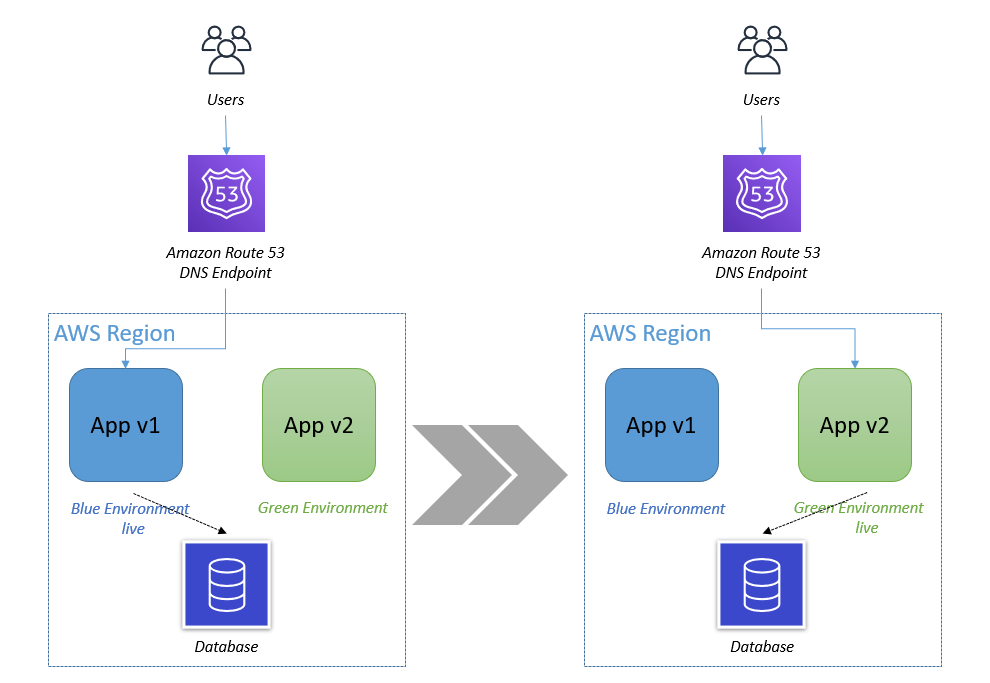
The example in this blog post uses a simplified structure with separate dedicated OUs and accounts for security and forensics, shown in Figure 1. Your organization’s architecture might differ, but the strategy remains the same.

Note: There might be reasons for forensic analysis to be performed live within the compromised account itself, such as to avoid shutting down or accessing the compromised instance or resource; however, that approach isn’t covered here.

Figure 1: AWS Organizations forensics OU example

Figure 1: AWS Organizations forensics OU example

The most important components in Figure 1 are:

  • A security OU, which is used for hosting security-related access and services. The security OU and the associated AWS accounts should be owned and managed by your security organization.
  • A forensics OU, which should be a separate entity, although it can have some similarities and crossover responsibilities with the security OU. There are several reasons for having it within a separate OU and account. Some of the more important reasons are that the forensics team might be a different team than the security team (or a subset of it), certain investigations might be under legal hold with additional access restrictions, or a member of the security team could be the focus of an investigation.

When speaking about Organizations, accounts, and the permissions required for various actions, you must first look at SCPs, a core functionality of Organizations. SCPs offer control over the maximum available permissions for all accounts in your organization. In the example in this blog post, you can use SCPs to provide similar or identical permission policies to all the accounts under the forensics OU, which is being used as a resource container. This policy overrides all other policies, and is a crucial mechanism to ensure that you can explicitly deny or allow any API calls desired. Some use cases of SCPs are to restrict the ability to disable AWS CloudTrail, restrict root user access, and ensure that all actions taken in the forensic investigation account are logged. This provides a centralized way to avoid changing individual policies for users, groups, or roles. Accessing the forensic environment should be done using a least-privilege model, with nobody capable of modifying or compromising the initially collected evidence. For an investigation environment, denying all actions except those you want to list as exceptions is the most straightforward approach. Start with the default of denying all, and work your way towards the least authorizations needed to perform the forensic processes established by your organization. AWS Config can be a valuable tool to track the changes made to the account and provide evidence of these changes.

Keep in mind that once the restrictive SCP is applied, even the root account or those with administrator access won’t have access beyond those permissions; therefore, frequent, proactive testing as your environment changes is a best practice. Also, be sure to validate which principals can remove the protective policy, if required, to transfer the account to an outside entity. Finally, create the environment before the restrictive permissions are applied, and then move the account under the forensic OU.

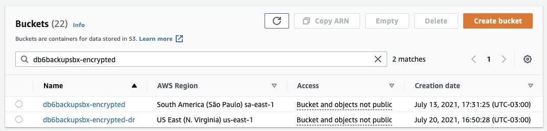
Having a separate AWS account dedicated to forensic investigations is best to keep your larger organization separate from the possible threat of contamination from the incident itself, ensure the isolation and protection of the integrity of the artifacts being analyzed, and keeping the investigation confidential. Separate accounts also avoid situations where the threat actors might have used all the resources immediately available to your compromised AWS account by hitting service quotas and so preventing you from instantiating an Amazon EC2 instance to perform investigations.

Having a forensic investigation account per Region is also a good practice, as it keeps the investigative capabilities close to the data being analyzed, reduces latency, and avoids issues of the data changing regulatory jurisdictions. For example, data residing in the EU might need to be examined by an investigative team in North America, but the data itself cannot be moved because its North American architecture doesn’t align with GDPR compliance. For global customers, forensics teams might be situated in different locations worldwide and have different processes. It’s better to have a forensic account in the Region where an incident arose. The account as a whole could also then be provided to local legal institutions or third-party auditors if required. That said, if your AWS infrastructure is contained within Regions only in one jurisdiction or country, then a single re-creatable account in one Region with evidence artifacts shared from and kept in their respective Regions could be an easier architecture to manage over time.

An account created in an automated fashion using a CloudFormation template—or other IaC methods—allows you to minimize human interaction before use by recreating an entirely new and untouched forensic analysis instance for each separate investigation, ensuring its integrity. Individual people will only be given access as part of a security incident response plan, and even then, permissions to change the environment should be minimal or none at all. The post-investigation environment would then be either preserved in a locked state or removed, and a fresh, blank one created in its place for the subsequent investigation with no trace of the previous artifacts. Templating your environment also facilitates testing to ensure your investigative strategy, permissions, and tooling will function as intended.

Accessing your forensics infrastructure

Once you’ve defined where your investigative environment should reside, you must think about who will be accessing it, how they will do so, and what permissions they will need.

The forensic investigation team can be a separate team from the security incident response team, the same team, or a subset. You should provide precise access rights to the group of individuals performing the investigation as part of maintaining least privilege.

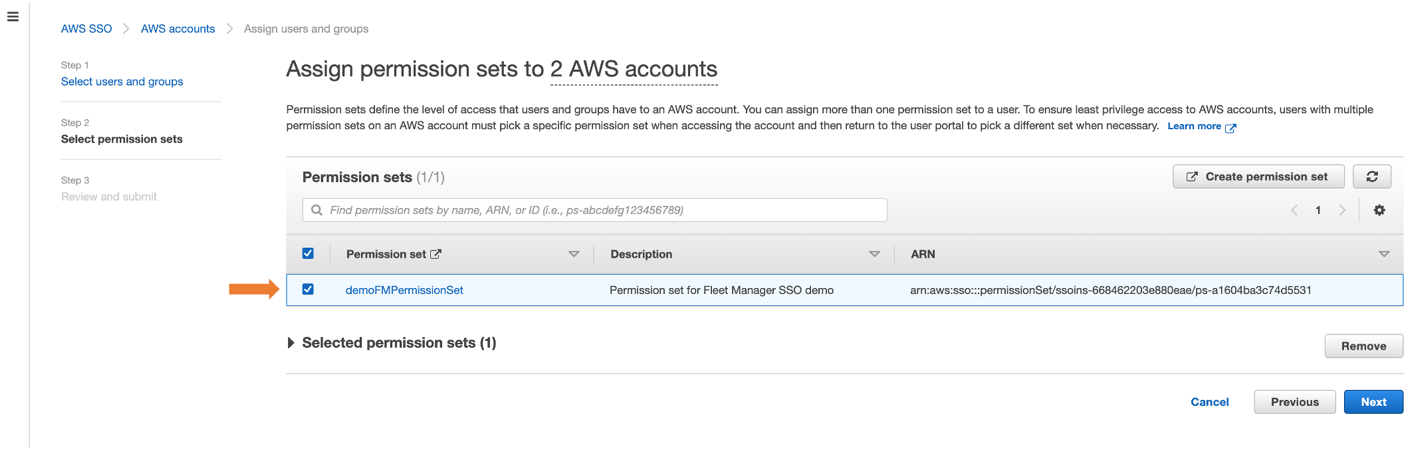
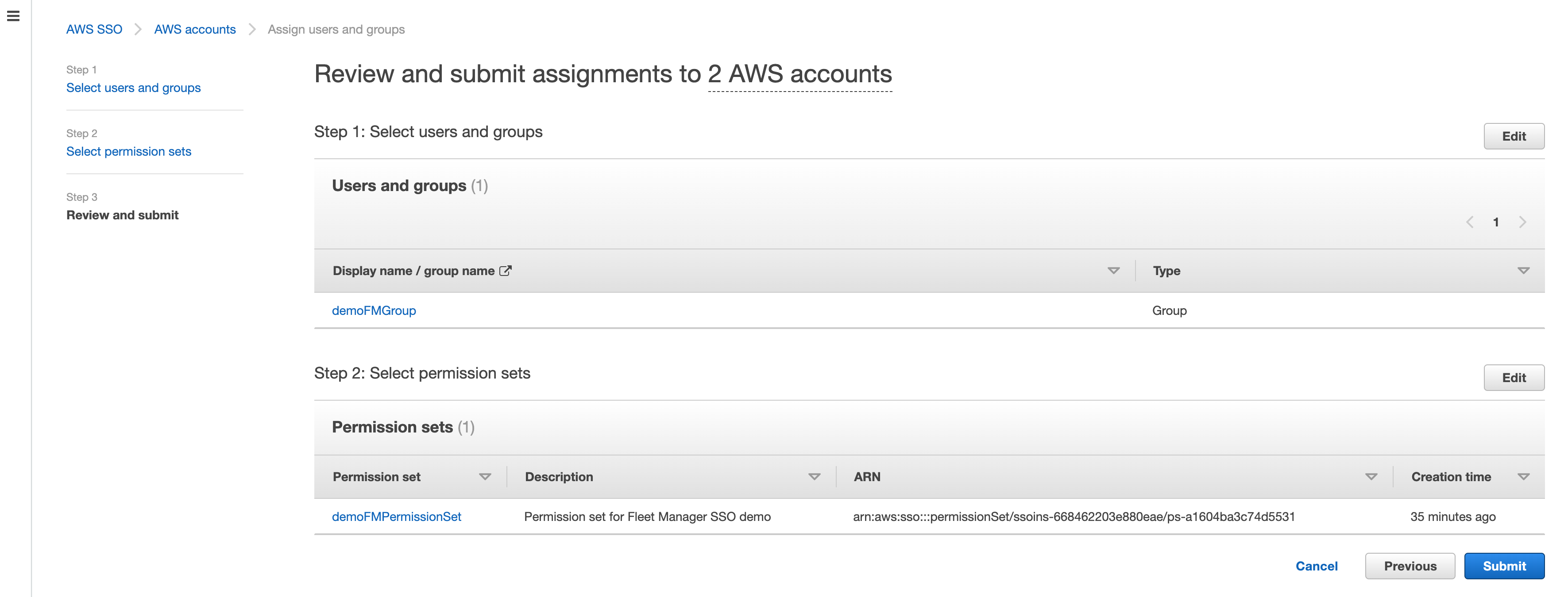
You should create specific roles for the various needs of the forensic procedures, each with only the permissions required. As with SCPs and other situations described here, start with no permissions and add authorizations only as required while establishing and testing your templated environments. As an example, you might create the following roles within the forensic account:

Responder – acquire evidence

Investigator – analyze evidence

Data custodian – manage (copy, move, delete, and expire) evidence

Analyst – access forensics reports for analytics, trends, and forecasting (threat intelligence)

You should establish an access procedure for each role, and include it in the response plan playbook. This will help you ensure least privilege access as well as environment integrity. For example, establish a process for an owner of the Security Incident Response Plan to verify and approve the request for access to the environment. Another alternative is the two-person rule. Alert on log-in is an additional security measure that you can add to help increase confidence in the environment’s integrity, and to monitor for unauthorized access.

You want the investigative role to have read-only access to the original evidence artifacts collected, generally consisting of Amazon Elastic Block Store (Amazon EBS) snapshots, memory dumps, logs, or other artifacts in an Amazon Simple Storage Service (Amazon S3) bucket. The original sources of evidence should be protected; MFA delete and S3 versioning are two methods for doing so. Work should be performed on copies of copies if rendering the original immutable isn’t possible, especially if any modification of the artifact will happen. This is discussed in further detail below.

Evidence should only be accessible from the roles that absolutely require access—that is, investigator and data custodian. To help prevent potential insider threat actors from being aware of the investigation, you should deny even read access from any roles not intended to access and analyze evidence.

Protecting the integrity of your forensic infrastructures

Once you’ve built the organization, account structure, and roles, you must decide on the best strategy inside the account itself. Analysis of the collected artifacts can be done through forensic analysis tools hosted on an EC2 instance, ideally residing within a dedicated Amazon VPC in the forensics account. This Amazon VPC should be configured with the same restrictive approach you’ve taken so far, being fully isolated and auditable, with the only resources being dedicated to the forensic tasks at hand.

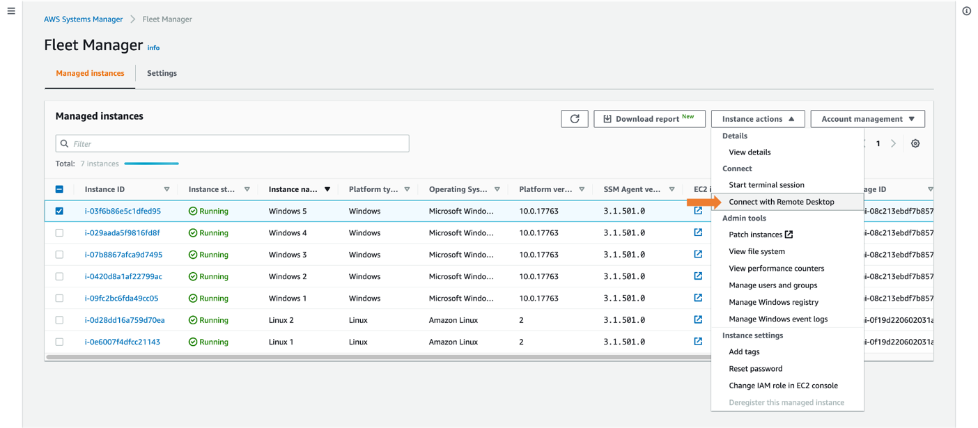
This might mean that the Amazon VPC’s subnets will have no internet gateways, and therefore all S3 access must be done through an S3 VPC endpoint. VPC flow logging should be enabled at the Amazon VPC level so that there are records of all network traffic. Security groups should be highly restrictive, and deny all ports that aren’t related to the requirements of the forensic tools. SSH and RDP access should be restricted and governed by auditable mechanisms such as a bastion host configured to log all connections and activity, AWS Systems Manager Session Manager, or similar.

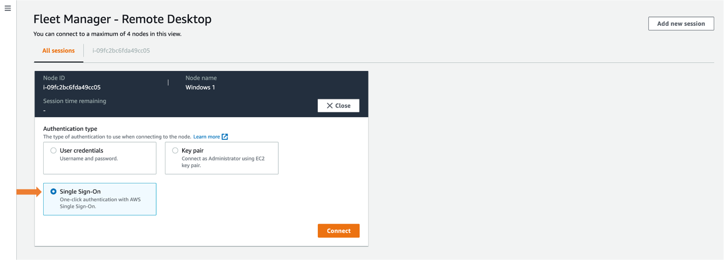
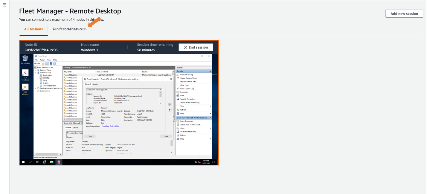
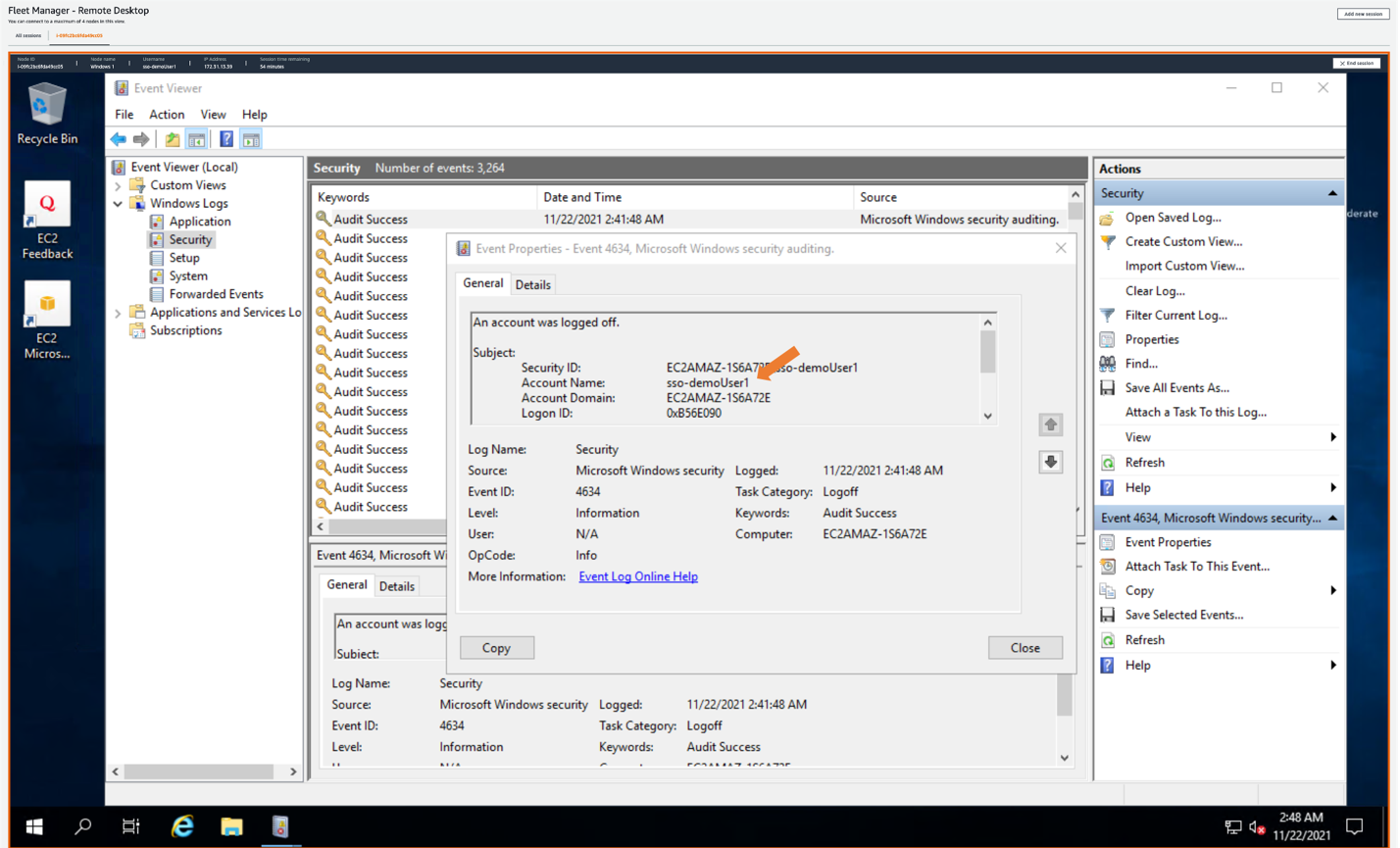
If using Systems Manager Session Manager with a graphical interface is required, RDP or other methods can still be accessed. Commands and responses performed using Session Manager can be logged to Amazon CloudWatch and an S3 bucket, this allows auditing of all commands executed on the forensic tooling Amazon EC2 instances. Administrative privileges can also be restricted if required. You can also arrange to receive an Amazon Simple Notification Service (Amazon SNS) notification when a new session is started.

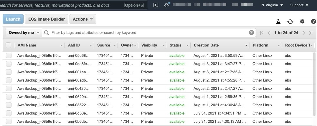
Given that the Amazon EC2 forensic tooling instances might not have direct access to the internet, you might need to create a process to preconfigure and deploy standardized Amazon Machine Images (AMIs) with the appropriate installed and updated set of tooling for analysis. Several best practices apply around this process. The OS of the AMI should be hardened to reduce its vulnerable surface. We do this by starting with an approved OS image, such as an AWS-provided AMI or one you have created and managed yourself. Then proceed to remove unwanted programs, packages, libraries, and other components. Ensure that all updates and patches—security and otherwise—have been applied. Configuring a host-based firewall is also a good precaution, as well as host-based intrusion detection tools. In addition, always ensure the attached disks are encrypted.

If your operating system is supported, we recommend creating golden images using EC2 Image Builder. Your golden image should be rebuilt and updated at least monthly, as you want to ensure it’s kept up to date with security patches and functionality.

EC2 Image Builder—combined with other tools—facilitates the hardening process; for example, allowing the creation of automated pipelines that produce Center for Internet Security (CIS) benchmark hardened AMIs. If you don’t want to maintain your own hardened images, you can find CIS benchmark hardened AMIs on the AWS Marketplace.

Keep in mind the infrastructure requirements for your forensic tools—such as minimum CPU, memory, storage, and networking requirements—before choosing an appropriate EC2 instance type. Though a variety of instance types are available, you’ll want to ensure that you’re keeping the right balance between cost and performance based on your minimum requirements and expected workloads.

The goal of this environment is to provide an efficient means to collect evidence, perform a comprehensive investigation, and effectively return to safe operations. Evidence is best acquired through the automated strategies discussed in How to automate incident response in the AWS Cloud for EC2 instances. Hashing evidence artifacts immediately upon acquisition is highly recommended in your evidence collection process. Hashes, and in turn the evidence itself, can then be validated after subsequent transfers and accesses, ensuring the integrity of the evidence is maintained. Preserving the original evidence is crucial if legal action is taken.

Evidence and artifacts can consist of, but aren’t limited to:

Access to the control plane logs mentioned above—such as the CloudTrail logs—can be accessed in one of two ways. Ideally, the logs should reside in a central location with read-only access for investigations as needed. However, if not centralized, read access can be given to the original logs within the source account as needed. Read access to certain service logs found within the security account, such as AWS Config, Amazon GuardDuty, Security Hub, and Amazon Detective, might be necessary to correlate indicators of compromise with evidence discovered during the analysis.

As previously mentioned, it’s imperative to have immutable versions of all evidence. This can be achieved in many ways, including but not limited to the following examples:

  • Amazon EBS snapshots, including hibernation generated memory dumps:
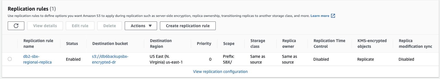
    • Original Amazon EBS disks are snapshotted, shared to the forensics account, used to create a volume, and then mounted as read-only for offline analysis.
  • Amazon EBS volumes manually captured:
    • Linux tools such as dc3dd can be used to stream a volume to an S3 bucket, as well as provide a hash, and then made immutable using an S3 method from the next bullet point.
  • Artifacts stored in an S3 bucket, such as memory dumps and other artifacts:
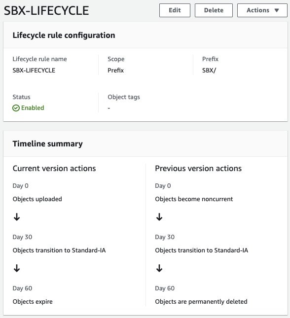
    • S3 Object Lock prevents objects from being deleted or overwritten for a fixed amount of time or indefinitely.
    • Using MFA delete requires the requestor to use multi-factor authentication to permanently delete an object.
    • Amazon S3 Glacier provides a Vault Lock function if you want to retain immutable evidence long term.
  • Disk volumes:
    • Linux: Mount in read-only mode.
    • Windows: Use one of the many commercial or open-source write-blocker applications available, some of which are specifically made for forensic use.
  • CloudTrail:
  • AWS Systems Manager inventory:
  • AWS Config data:
    • By default, AWS Config stores data in an S3 bucket, and can be protected using the above methods.

Note: AWS services such as KMS can help enable encryption. KMS is integrated with AWS services to simplify using your keys to encrypt data across your AWS workloads.

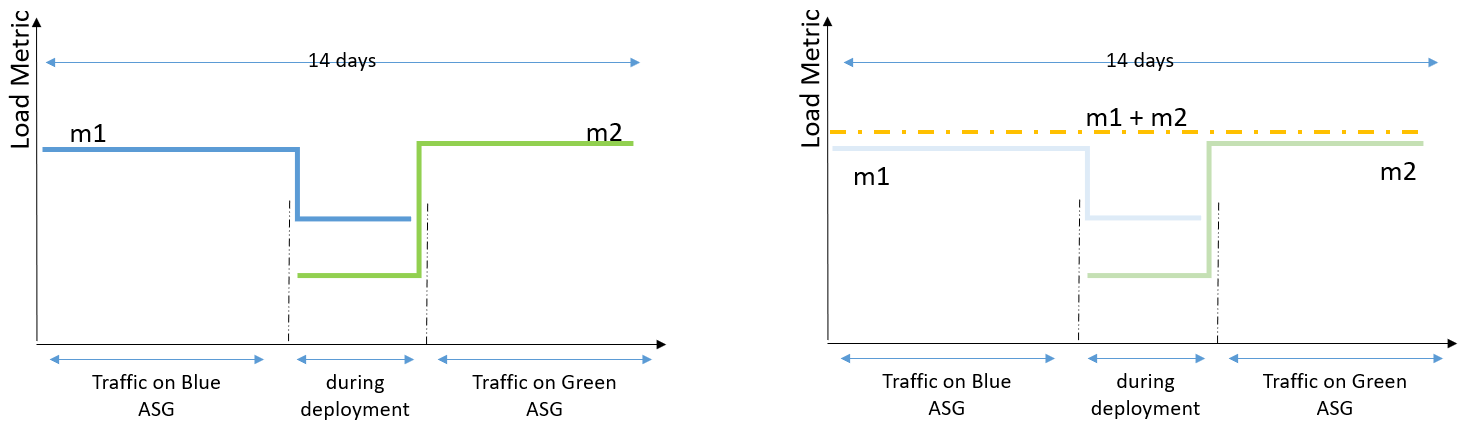
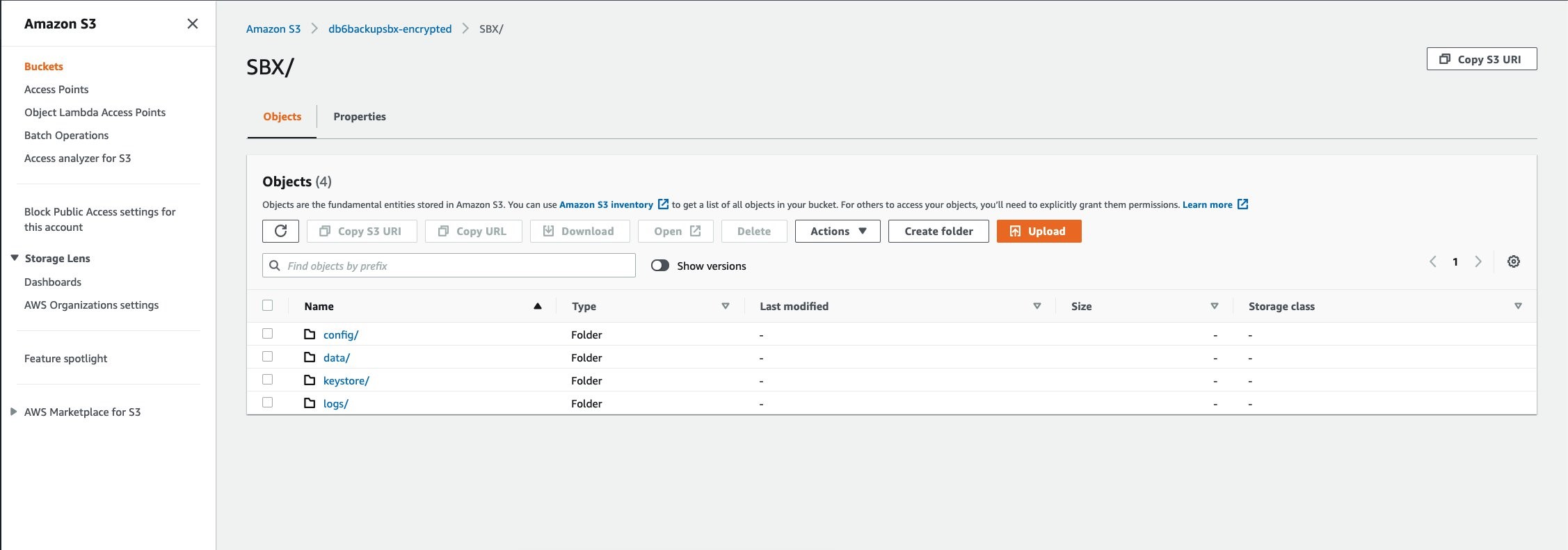
An example use case of Amazon EBS disks being shared as evidence to the forensics account, the following figure—Figure 2—is a simplified S3 bucket folder structure you could use to store and work with evidence.

Figure 2 shows an S3 bucket structure for a forensic account. An S3 bucket and folder is created to hold incoming data—for example, from Amazon EBS disks—which is streamed to Incoming Data > Evidence Artifacts using dc3dd. The data is then copied from there to a folder in another bucket—Active Investigation > Root Directory > Extracted Artifacts—to be analyzed by the tooling installed on your forensic Amazon EC2 instance. Also, there are folders under Active Investigation for any investigation notes you make during analysis, as well as the final reports, which are discussed at the end of this blog post. Finally, a bucket and folders for legal holds, where an object lock will be placed to hold evidence artifacts at a specific version.

Figure 2: Forensic account S3 bucket structure

Figure 2: Forensic account S3 bucket structure

Considerations

Finally, depending on the severity of the incident, your on-premises network and infrastructure might also be compromised. Having an alternative environment for your security responders to use in case of such an event reduces the chance of not being able to respond in an emergency. Amazon services such as Amazon Workspaces—a fully managed persistent desktop virtualization service—can be used to provide your responders a ready-to-use, independent environment that they can use to access the digital forensics and incident response tools needed to perform incident-related tasks.

Aside from the investigative tools, communications services are among the most critical for coordination of response. You can use Amazon WorkMail and Amazon Chime to provide that capability independent of normal channels.

Conclusion

The goal of a forensic investigation is to provide a final report that’s supported by the evidence. This includes what was accessed, who might have accessed it, how it was accessed, whether any data was exfiltrated, and so on. This report might be necessary for legal circumstances, such as criminal or civil investigations or situations requiring breach notifications. What output each circumstance requires should be determined in advance in order to develop an appropriate response and reporting process for each. A root cause analysis is vital in providing the information required to prepare your resources and environment to help prevent a similar incident in the future. Reports should not only include a root cause analysis, but also provide the methods, steps, and tools used to arrive at the conclusions.

This article has shown you how you can get started creating and maintaining forensic environments, as well as enable your teams to perform advanced incident resolution investigations using AWS services. Implementing the groundwork for your forensics environment, as described above, allows you to use automated disk collection to begin iterating on your forensic data collection capabilities and be better prepared when security events occur.

If you have feedback about this post, submit comments in the Comments section below. If you have questions about this post, start a new thread on one of the AWS Security, Identity, and Compliance forums or contact AWS Support.

Want more AWS Security how-to content, news, and feature announcements? Follow us on Twitter.

Author

Sol Kavanagh

Sol is a senior solutions architect and CISSP with 20+ years of experience in the enterprise space. He is passionate about security and helping customers build solutions in the AWS Cloud. In his spare time he enjoys distance cycling, adventure travelling, Buddhist philosophy, and Muay Thai.

Identifying optimal locations for flexible workloads with Spot placement score

Post Syndicated from Pranaya Anshu original https://aws.amazon.com/blogs/compute/identifying-optimal-locations-for-flexible-workloads-with-spot-placement-score/

This post is written by Jessie Xie, Solutions Architect for EC2 Spot, and Peter Manastyrny, Senior Product Manager for EC2 Auto Scaling and EC2 Fleet.

Amazon EC2 Spot Instances let you run flexible, fault-tolerant, or stateless applications in the AWS Cloud at up to a 90% discount from On-Demand prices. Since we introduced Spot Instances back in 2009, we have been building new features and integrations with a single goal – to make Spot easy and efficient to use for your flexible compute needs.

Spot Instances are spare EC2 compute capacity in the AWS Cloud available for steep discounts. In exchange for the discount, Spot Instances are interruptible and must be returned when EC2 needs the capacity back. The location and amount of spare capacity available at any given moment is dynamic and changes in real time. This is why Spot workloads should be flexible, meaning they can utilize a variety of different EC2 instance types and can be shifted in real time to where the spare capacity currently is. You can use Spot Instances with tools such as EC2 Fleet and Amazon EC2 Auto Scaling which make it easy to run workloads on multiple instance types.

The AWS Cloud spans 81 Availability Zones across 25 Regions with plans to launch 21 more Availability Zones and 7 more Regions. However, until now there was no way to find an optimal location (either a Region or Availability Zone) to fulfill your Spot capacity needs without trying to launch Spot Instances there first. Today, we are excited to announce Spot placement score, a new feature that helps you identify an optimal location to run your workloads on Spot Instances. Spot placement score recommends an optimal Region or Availability Zone based on the amount of Spot capacity you need and your instance type requirements.

Spot placement score is useful for workloads that could potentially run in a different Region. Additionally, because the score takes into account your instance type selection, it can help you determine if your request is sufficiently instance type flexible for your chosen Region or Availability Zone.

How Spot placement score works

To use Spot placement score you need to specify the amount of Spot capacity you need, what your instance type requirements are, and whether you would like a recommendation for a Region or a single Availability Zone. For instance type requirements, you can either provide a list of instance types, or the instance attributes, like the number of vCPUs and amount of memory. If you choose to use the instance attributes option, you can then use the same attribute configuration to request your Spot Instances in the recommended Region or Availability Zone with the new attribute-based instance type selection feature in EC2 Fleet or EC2 Auto Scaling.

Spot placement score provides a list of Regions or Availability Zones, each scored from 1 to 10, based on factors such as the requested instance types, target capacity, historical and current Spot usage trends, and time of the request. The score reflects the likelihood of success when provisioning Spot capacity, with a 10 meaning that the request is highly likely to succeed. Provided scores change based on the current Spot capacity situation, and the same request can yield different scores when ran at different times. It is important to note that the score serves as a guideline, and no score guarantees that your Spot request will be fully or partially fulfilled.

You can also filter your score by Regions or Availability Zones, which is useful for cases where you can use only a subset of AWS Regions, for example any Region in the United States.

Let’s see how Spot placement score works in practice through an example.

Using Spot placement score with AWS Management Console

To try Spot placement score, log into your AWS account, select EC2, Spot Requests, and click on Spot placement score to open the Spot placement score window.

Spot placement score screen in AWS Management Console.

Here, you need provide your target capacity and instance type requirements by clicking on Enter requirements. You can enter target capacity as a number of instances, vCPUs, or memory. vCPUs and memory options are useful for vertically scalable workloads that are sized for a total amount of compute resources and can utilize a wide range of instance sizes. Target capacity is limited and based on your recent Spot usage with accounting for potential usage growth. For accounts that do not have recent Spot usage, there is a default limit aligned with the Spot Instances limit.

For instance type requirements, there are two options. First option is to select Specify instance attributes that match your compute requirements tab and enter your compute requirements as a number of vCPUs, amount of memory, CPU architecture, and other optional attributes. Second option is to select Manually select instance types tab and select instance types from the list.

Please note that you need to select at least three different instance types (that is, different families, generations, or sizes). If you specify a smaller number of instance types, Spot placement score will always yield a low score. Spot placement score is designed to help you find an optimal location to request Spot capacity tailored to your specific workload needs, but it is not intended to be used for getting high-level Spot capacity information across all Regions and instance types.

Let’s try to find an optimal location to run a workload that can utilize r5.8xlarge, c5.9xlarge, and m5.8xlarge instance types and is sized at 2000 instances.

Spot placement score screen in AWS Management Console with selected target capacity at 2000 instances and selected r5.8xlarge, c5.9xlarge, and m5.8xlarge instance types..

Once you select 2000 instances under Target capacity, select r5.8xlarge, c5.9xlarge, and m5.8xlarge instances under Select instance types, and click Load placement score button, you will get a list of Regions sorted by score in a descending order. There is also an option to filter by specific Regions if needed.

The highest rated Region for your requirements turns out to be US East (N. Virginia) with a score of 8. The second closest contender is Europe (Ireland) with a score of 5. That tells you that right now the optimal Region for your Spot requirements is US East (N. Virginia).

Spot placement score screen in AWS Management Console with displayed scores on Region level scores.

Let’s now see if it is possible to get a higher score. Remember, the key best practice for Spot is to be flexible and utilize as many instance types as possible. To do that, press the Edit button on the Target capacity and instance type requirements tab. For the new request, keep the same target capacity at 2000, but expand the selection of instance types by adding similarly sized instance types from a variety of instance families and generations, i.e., r5.4xlarge, r5.12xlarge, m5zn.12xlarge, m5zn.6xlarge, m5n.8xlarge, m5dn.8xlarge, m5d.8xlarge, r5n.8xlarge, r5dn.8xlarge, r5d.8xlarge, c5.12xlarge, c5.4xlarge, c5d.12xlarge, c5n.9xlarge. c5d.9xlarge, m4.4xlarge, m4.16xlarge, m4.10xlarge, r4.8xlarge, c4.8xlarge.

After requesting the scores with updated requirements, you can see that even though the score in US East (N. Virginia) stays unchanged at 8, the scores for Europe (Ireland) and US West (Oregon) improved dramatically, both raising to 9. Now, you have a choice of three high-scored Regions to request your Spot Instances, each with a high likelihood to succeed.

To request Spot Instances based on the score, you can use EC2 Fleet or EC2 Auto Scaling. Please note, that the score implies that you use capacity-optimized Spot allocation strategy when requesting the capacity. If you use other allocation strategies, such as lowest-price, the result in the recommended Region or Availability Zone will not align with the score provided.

Spot placement score screen in AWS Management Console with selected target capacity at 2000 instances and selected r5.8xlarge, c5.9xlarge, m5.8xlarge, r5.4xlarge, r5.12xlarge, m5zn.12xlarge, m5zn.6xlarge, m5n.8xlarge, m5dn.8xlarge, m5d.8xlarge, r5n.8xlarge, r5dn.8xlarge, r5d.8xlarge, c5.12xlarge, c5.4xlarge, c5d.12xlarge, c5n.9xlarge. c5d.9xlarge, m4.4xlarge, m4.16xlarge, m4.10xlarge, r4.8xlarge, c4.8xlarge instance types.

You can also request the scores at the Availability Zone level. This is useful for running workloads that need to have all instances in the same Availability Zone, potentially to minimize inter-Availability Zone data transfer costs. Workloads such as Apache Spark, which involve transferring a high volume of data between instances, would be a good use case for this. To get scores per Availability Zone you can check the box Provide placement scores per Availability Zone.

When requesting instances based on Availability Zone recommendation, you need to make sure to configure EC2 Fleet or EC2 Auto Scaling request to only use that specific Availability Zone.

With Spot placement score, you can test different instance type combinations at different points in time, and find the most optimal Region or Availability Zone to run your workloads on Spot Instances.

Availability and pricing

You can use Spot placement score today in all public and AWS GovCloud Regions with the exception of those based in China, where we plan to release later. You can access Spot placement score using the AWS Command Line Interface (CLI), AWS SDKs, and Management Console. There is no additional charge for using Spot placement score, you will only pay EC2 standard rates if provisioning instances based on recommendation.

To learn more about using Spot placement score, visit the Spot placement score documentation page. To learn more about best practices for using Spot Instances, see Spot documentation.

New – Attribute-Based Instance Type Selection for EC2 Auto Scaling and EC2 Fleet

Post Syndicated from Danilo Poccia original https://aws.amazon.com/blogs/aws/new-attribute-based-instance-type-selection-for-ec2-auto-scaling-and-ec2-fleet/

The first AWS service I used, more than ten years ago, was Amazon Elastic Compute Cloud (Amazon EC2). Over time, EC2 has added a wide selection of instance types optimized to fit different use cases, with a varying combination of CPU/GPU, memory, storage, and networking capacity to give you the flexibility to choose the appropriate mix of resources for your applications.

One of the key advantages of the cloud is elasticity. With EC2 Fleet, you can synchronously request capacity across multiple instance types and purchase options, launching your instances across multiple Availability Zones, using the On-Demand, Reserved, and Spot Instances together. With EC2 Auto Scaling, you can automatically add or remove EC2 instances according to conditions you define and add advanced instance management capabilities such as warm pools, instance refresh, and health checks. With these tools, you need to manually update your configurations to benefit from the newest EC2 instances. Also, when you use EC2 Spot Instances to optimize your costs, it is important that you select multiple instance types to access the highest amount of Spot capacity. Until now, there was no easy way to build and maintain instance type configurations in a flexible way.

Today, I am happy to share that we are introducing attribute-based instance type selection (ABS), a new feature that lets you express your instance requirements as a set of attributes, such as vCPU, memory, and storage. Your requirements are translated by ABS to all matching instance types, simplifying the creation and maintenance of instance type configurations. This also allows you to automatically use newer generation instance types when they are released and access a broader range of capacity via EC2 Spot Instances. EC2 Fleet and EC2 Auto Scaling select and launch instances that fit the specified attributes, removing the need to manually pick instance types.

ABS is ideal for flexible workloads and frameworks, such as when running containers or web fleets, processing big data, and implementing continuous integration and deployment (CI/CD) tooling. When using Spot Instances, instead of picking and entering tens of instance types and sizes, you can now just use a simple attribute config to cover all of them and include new ones as they come out.

How Attribute-Based Instance Type Selection Works
With ABS, you replace the list of instance types with your instance requirements. You can specify instance requirements inside a launch template or in the EC2 Fleet or EC2 Auto Scaling requests as a launch template override.

ABS works in two steps:

  • First, ABS determines a list of instance types based on specified attributes, AWS Region, Availability Zone, and price.
  • Then, EC2 Auto Scaling or EC2 Fleet applies the selected allocation strategy to that list.

For Spot Instances, ABS supports the capacity-optimized and the lowest-price allocation strategies.

For On-Demand Instances, ABS supports the lowest-price allocation strategy. EC2 Auto Scaling or EC2 Fleet will resolve ABS attributes to a list of instance types and will launch the lowest priced instance first to fulfill the On-Demand portion of the capacity request, moving to the next lowest priced instance if needed.

By default ABS enables price protection to keep your spending under control. Price protection makes ABS avoid provisioning overly expensive instance types even if they happen to fit the attributes you selected and keeps the prices of provisioned instances within certain boundaries. With price protection enabled, ABS doesn’t select instance types whose price is above price protection thresholds. There are two separate thresholds for Spot and On-Demand instances that you can optionally customize.

Let’s see how ABS works in practice with a couple of examples.

Using Attribute-Based Instance Type Selection with EC2 Auto Scaling
I use the AWS Command Line Interface (CLI) with the --generate-cli-skeleton parameter to generate a file in YAML format with all the parameters accepted by the CreateAutoScalingGroup API.

aws autoscaling create-auto-scaling-group \
    --generate-cli-skeleton yaml-input > create-asg.yaml

In the YAML file, there is a new InstanceRequirements section that can be used to override the configuration of the launch template. These are all the attributes I can choose from with some sample values:

InstanceRequirements:
  VCpuCount:  # [REQUIRED] 
    Min: 0
    Max: 0
  MemoryMiB: # [REQUIRED] 
    Min: 0
    Max: 0
  CpuManufacturers:
  - amd
  MemoryGiBPerVCpu:
    Min: 0.0
    Max: 0.0
  ExcludedInstanceTypes:
  - ''
  InstanceGenerations:
  - previous
  SpotMaxPricePercentageOverLowestPrice: 0
  OnDemandMaxPricePercentageOverLowestPrice: 0
  BareMetal: required  #  Valid values are: included, excluded, required.
  BurstablePerformance: excluded #  Valid values are: included, excluded, required.
  RequireHibernateSupport: true
  NetworkInterfaceCount:
    Min: 0
    Max: 0
  LocalStorage: required  #  Valid values are: included, excluded, required.
  LocalStorageTypes:
  - ssd
  TotalLocalStorageGB:
    Min: 0.0
    Max: 0.0
  BaselineEbsBandwidthMbps:
    Min: 0
    Max: 0
  AcceleratorTypes:
  - inference
  AcceleratorCount:
    Min: 0
    Max: 0
  AcceleratorManufacturers:
  - amazon-web-services
  AcceleratorNames:
  - a100
  AcceleratorTotalMemoryMiB:
    Min: 0
    Max: 0

Instead of providing a list of overrides, each having an InstanceType attribute with a single instance type selected, I can now select the instance types based on my requirements. I can specify the minimum and maximum amount of vCPUs, and the range of memory. Optionally, I can ask for a minimum amount of memory per vCPUs.

There are many more attributes that I can select from. For example, I can include, exclude, or require the use of bare metal or burstable instances. I can add networking or storage requirements. If necessary, I can ask for GPU or FPGA accelerators, and so on.

In my case, I ask for instances with two to four vCPUs and at least 2048 MiB of memory. Previously, it would have taken about 40 overrides, one for each instance type that meets these requirements, but with ABS, I just have to specify three parameters in the InstanceRequirements section. This is the full configuration file I am going to use to create the Auto Scaling group:

AutoScalingGroupName: 'my-asg' # [REQUIRED] 
MixedInstancesPolicy:
  LaunchTemplate:
    LaunchTemplateSpecification:
      LaunchTemplateId: 'lt-0537239d9aef10a77'
    Overrides:
    - InstanceRequirements:
        VCpuCount: # [REQUIRED] 
          Min: 2
          Max: 4
        MemoryMiB: # [REQUIRED] 
          Min: 2048
  InstancesDistribution:
    OnDemandPercentageAboveBaseCapacity: 50
    SpotAllocationStrategy: 'capacity-optimized'
MinSize: 0 # [REQUIRED] 
MaxSize: 100 # [REQUIRED] 
DesiredCapacity: 4
VPCZoneIdentifier: 'subnet-e76a128a,subnet-e66a128b,subnet-e16a128c'

I create the Auto Scaling group passing the configuration file with the --cli-input-yaml parameter:

aws autoscaling create-auto-scaling-group \
    --cli-input-yaml file://my-create-asg.yaml

After a few minutes, four EC2 instances (corresponding to my DesiredCapacity) are running in the EC2 console. In the list, I find both C3 and C5a instances, spanning both time and CPU manufacturer.

Console screenshot.

Of those instances, 50 percent is On-Demand (based on the OnDemandPercentageAboveBaseCapacity option in the InstancesDistribution section). In the Spot Request tab of the EC2 console, I see the two requests:

Console screenshot.

As expected, all instance types follow my requirements and have size large. However, I quickly realize my application needs more compute capacity in each instance. I update the Auto Scaling group with the new requirements, asking for more vCPUs (between four and six):

aws autoscaling update-auto-scaling-group \
    --auto-scaling-group-name my-asg \
    --mixed-instances-policy '{
        "LaunchTemplate": {
            "Overrides": [
                {
                    "InstanceRequirements": {
                    "VCpuCount":{"Min": 4, "Max": 6},
                    "MemoryMiB":{"Min": 2048} }
                } ]
        } }' 

Then, I start the instance refresh of the Auto Scaling group:

aws autoscaling start-instance-refresh \
    --auto-scaling-group-name my-asg

EC2 Auto Scaling performs a rolling replacement of the instances based on the new requirements. After a few minutes, all instances have been replaced by new ones with size xlarge, and I have a mix of C5, C5a, and M3 instances running. All previous instances have been terminated.

Console screenshot.

Similar to before, two of the new instances are launched using Spot requests. The previous Spot requests have been closed.

Console screenshot.

How to Preview Matching Instances without Launching Them
To better understand how the new ABS works, I use the new EC2 GetInstanceTypesFromInstanceRequirements API. This API returns the list of instance types matching my requirements.

First, I create the YAML parameter file:

aws ec2 get-instance-types-from-instance-requirements --generate-cli-skeleton yaml-input > requirements.yaml

I edit the file with the same requirements I used to update the Auto Scaling group. This time, I also ask to use current generation instances:

ArchitectureTypes:  # [REQUIRED] 
- x86_64
VirtualizationTypes: # [REQUIRED] 
- hvm
InstanceRequirements: # [REQUIRED] 
  VCpuCount:
    Min: 4
    Max: 6
  MemoryMiB:
    Min: 2048
  InstanceGenerations:
    - current

Note that here I had to specify the type of architecture (x86_64) and virtualization (hvm). When creating the Auto Scaling group, this information was provided by the Amazon Machine Images (AMI) used by the launch template.

Now, let’s preview all the instance types selected by these requirements:

aws ec2 get-instance-types-from-instance-requirements \
    --cli-input-yaml file://requirements.yaml \
    --output table

------------------------------------------
|GetInstanceTypesFromInstanceRequirements|
+----------------------------------------+
||             InstanceTypes            ||
|+--------------------------------------+|
||             InstanceType             ||
|+--------------------------------------+|
||  c4.xlarge                           ||
||  c5.xlarge                           ||
||  c5a.xlarge                          ||
||  c5ad.xlarge                         ||
||  c5d.xlarge                          ||
||  c5n.xlarge                          ||
||  d2.xlarge                           ||
||  d3.xlarge                           ||
||  d3en.xlarge                         ||
||  g3s.xlarge                          ||
||  g4ad.xlarge                         ||
||  g4dn.xlarge                         ||
||  i3.xlarge                           ||
||  i3en.xlarge                         ||
||  inf1.xlarge                         ||
||  m4.xlarge                           ||
||  m5.xlarge                           ||
||  m5a.xlarge                          ||
||  m5ad.xlarge                         ||
||  m5d.xlarge                          ||
||  m5dn.xlarge                         ||
||  m5n.xlarge                          ||
||  m5zn.xlarge                         ||
||  m6i.xlarge                          ||
||  p2.xlarge                           ||
||  r4.xlarge                           ||
||  r5.xlarge                           ||
||  r5a.xlarge                          ||
||  r5ad.xlarge                         ||
||  r5b.xlarge                          ||
||  r5d.xlarge                          ||
||  r5dn.xlarge                         ||
||  r5n.xlarge                          ||
||  x1e.xlarge                          ||
||  z1d.xlarge                          ||
|+--------------------------------------+|

Using this new EC2 API, I can quickly test different requirements and see how they map to instance types. When new instance types are released, they are automatically added to the list if they match my requirements.

Availability and Pricing
You can use attribute-based instance type selection (ABS) with EC2 Auto Scaling and EC2 Fleet today in all public and GovCloud AWS Regions, with the exception of those based in China where we need more time. You can configure ABS using the AWS Command Line Interface (CLI), AWS SDKs, AWS Management Console, and AWS CloudFormation. There is no additional charge for using ABS; you only pay the standard EC2 pricing for the provisioned instances. For more information on price protection, see the EC2 Auto Scaling documentation.

This new feature makes it easy to use flexible instance type configurations instead of long lists of instance types. In this way, you can automatically use newer generation instance types when they are released in the Region. Also, you can easily access more capacity with your Spot requests.

Simplify your EC2 instance type configurations with attribute-based instance type selection.

Danilo

New – EC2 Instances Powered by Gaudi Accelerators for Training Deep Learning Models

Post Syndicated from Jeff Barr original https://aws.amazon.com/blogs/aws/new-ec2-instances-powered-by-gaudi-accelerators-for-training-deep-learning-models/

There are more applications today for deep learning than ever before. Natural language processing, recommendation systems, image recognition, video recognition, and more can all benefit from high-quality, well-trained models.

The process of building such a model is iterative: construct an initial model, train it on the ground truth data, do some test inferences, refine the model and repeat. Deep learning models contain many layers (hence the name), each of which transforms outputs of the previous layer. The training process is math and processor intensive, and places demands on just about every part of the systems used for training including the GPU or other training accelerator, the network, and local or network storage. This sophistication and complexity increases training time and raises costs.

New DL1 Instances
Today I would like to tell you about our new DL1 instances. Powered by Gaudi accelerators from Habana Labs, the dl1.24xlarge instances have the following specs:

Gaudi Accelerators – Each instance is equipped with eight Gaudi accelerators, with a total of 256 GB of High Bandwidth (HBM2) accelerator memory and high-speed, RDMA-powered communication between accelerators.

System Memory – 768 GB of system memory, enough to hold very large sets of training data in memory, as often requested by our customers.

Local Storage – 4 TB of local NVMe storage, configured as four 1 TB volumes.

Processor – Intel Cascade Lake processor with 96 vCPUs.

Network – 400 Gbps of network throughput.

As you can see, we have maxed out the specs in just about every dimension, with the goal of giving you a highly capable machine learning training platform with a low cost of entry and up to 40% better price-performance than current GPU-based EC2 instances.

Gaudi Inside
The Gaudi accelerators are custom-designed for machine learning training, and have a ton of cool & interesting features & attributes:

Data Types – Support for floating point (BF16 and FP32), signed integer (INT8, INT16, and INT32), and unsigned integer (UINT8, UINT16, and UINT32) data.

Generalized Matrix Multiplier Engine (GEMM) – Specialized hardware to accelerate matrix multiplication.

Tensor Processing Cores (TPCs) – Specialized VLIW SIMD (Very Long Instruction Word / Single Instruction Multiple Data) processing units designed for ML training. The TPCs are C-programmable, although most users will use higher-level tools and frameworks.

Getting Started with DL1 Instances
The Gaudi SynapseAI Software Suite for Training will help you to build new models and to migrate existing models from popular frameworks such as PyTorch and TensorFlow:

Here are some resources to get you started:

TensorFlow User Guide – Learn how to run your TensorFlow models on Gaudi.

PyTorch User Guide – Learn how to run your PyTorch models on Gaudi.

Gaudi Model Migration Guide – Learn how to port your PyTorch or TensorFlow to Gaudi.

HabanaAI Repo – This large, active repo contains setup instructions, reference models, academic papers, and much more.

You can use the TPC Programming Tools to write, simulate, and debug code that runs directly on the TPCs, and you can use the Habana Communication Library (HCL) to build applications that harness the power of multiple accelerators. The Habana Collective Communications Library (HCCL) runs atop HCL and gives you access to collective primitives for Reduce, Broadcast, Gather, and Scatter operations.

Now Available
DL1 instances are available today in the US East (N. Virginia) and US West (Oregon) Regions in On-Demand and Spot form. You can purchase Reserved Instances and Savings plans as well.

Jeff;

Optimizing your AWS Infrastructure for Sustainability, Part III: Networking

Post Syndicated from Katja Philipp original https://aws.amazon.com/blogs/architecture/optimizing-your-aws-infrastructure-for-sustainability-part-iii-networking/

In Part I: Compute and Part II: Storage of this series, we introduced strategies to optimize the compute and storage layer of your AWS architecture for sustainability.

This blog post focuses on the network layer of your AWS infrastructure and proposes concepts to optimize your network utilization.

Optimizing the networking layer of your AWS infrastructure

When you make your applications available to more customers, the packets that travel across the network will increase. Similarly, the larger the size of data, as well as the more distance a packet has to travel, the more resources are required to transmit it. With growing number of application users, optimizing network traffic can ensure that network resource consumption is not growing linearly.

The recommendations in the following sections will help you use your resources more efficiently for the network layer of your workload.

Reducing the network traveled per request

Reducing the data sent over the network and optimizing the path a packet takes will result in a more efficient data transfer. The following table provides metrics related to some AWS services that can help you find potential network optimization opportunities.

Service Metric/Check Source
Amazon CloudFront Cache hit rate Viewing CloudFront and Lambda@Edge metrics
AWS Trusted Advisor check reference
Amazon Simple Storage Service (Amazon S3) Data transferred in/out of a bucket Metrics and dimensions
AWS Trusted Advisor check reference
Amazon Elastic Compute Cloud (Amazon EC2) NetworkPacketsIn/NetworkPacketsOut List the available CloudWatch metrics for your instances
AWS Trusted Advisor CloudFront Content Delivery Optimization AWS Trusted Advisor check reference

We recommend the following concepts to optimize your network utilization.

Read local, write global

The following strategies allow users to read the data from the source closest to them; thus, fewer requests travel longer distances.

  • If you are operating within a single AWS Region, you should choose a Region that is near the majority of your users. The further your users are away from the Region, the further data needs to travel through the global network.
  • If your users are spread over multiple Regions, set up multiple copies of the data to reside in each Region. Amazon Relational Database Service (Amazon RDS) and Amazon Aurora let you set up cross-Region read replicas. Amazon DynamoDB global tables allow for fast performance and alleviate network load.

Use a content delivery network

Content delivery networks (CDNs) bring your data closer to the end user. When requested, they cache static content from the original server and deliver it to the user. This shortens the distance each packet has to travel.

  • CloudFront optimizes network utilization and delivers traffic over CloudFront’s globally distributed edge network. Figure 1 shows a global user base that accesses an S3 bucket directly versus serving cached data from edge locations.
  • Trusted Advisor includes a check that recommends whether you should use a CDN for your S3 buckets. It analyzes the data transferred out of your S3 bucket and flags the buckets that could benefit from a CloudFront distribution.
Comparison of accessing an S3 bucket directly versus via a CloudFront distribution/edge locations

Figure 1. Comparison of accessing an S3 bucket directly versus via a CloudFront distribution/edge locations

Optimize CloudFront cache hit ratio

CloudFront caches different versions of an object depending upon the request headers (for example, language, date, or user-agent). You can further optimize your CDN distribution’s cache hit ratio (the number of times an object is served from the CDN versus from the origin) with a Trusted Advisor check. It automatically checks for headers that do not affect the object and then recommends a configuration to ignore those headers and not forward the request to the origin.

Use edge-oriented services

Edge computing brings data storage and computation closer to users. By implementing this approach, you can perform data preprocessing or run machine learning algorithms on the edge.

  • Edge-oriented services applied on gateways or directly onto user devices reduce network traffic because data does not need to be sent back to the cloud server.
  • One-time, low-latency tasks are a good fit for edge use cases, like when an autonomous vehicle needs to detect objects nearby. You should generally archive data that needs to be accessed by multiple parties in the cloud, but consider factors such as device hardware and privacy regulations first.
  • CloudFront Functions can run compute on edge locations and Lambda@Edge can generate Regional edge caches. AWS IoT Greengrass provides edge computing for Internet of Things (IoT) devices.

Reducing the size of data transmitted

Serve compressed files

In addition to caching static assets, you can further optimize network utilization by serving compressed files to your users. You can configure CloudFront to automatically compress objects, which results in faster downloads, leading to faster rendering of webpages.

Enhance Amazon EC2 network performance

Network packets consist of data that you are sending (frame) and the processing overhead information. If you use larger packets, you can pass more data in a single packet and decrease processing overhead.

Jumbo frames use the largest permissible packet that can be passed over the connection. Keep in mind that outside a single virtual private cloud (VPC), over virtual private network (VPN) or internet gateway, traffic is limited to a lower frame regardless of using jumbo frames.

Optimize APIs

If your payloads are large, consider reducing their size to reduce network traffic by compressing your messages for your REST API payloads. Use the right endpoint for your use case. Edge-optimized API endpoints are best suited for geographically distributed clients. Regional API endpoints are best suited for when you have a few clients with higher demands, because they can help reduce connection overhead. Caching your API responses will reduce network traffic and enhance responsiveness.

Conclusion

As your organization’s cloud adoption grows, knowing how efficient your resources are is crucial when optimizing your AWS infrastructure for environmental sustainability. Using the fewest number of resources possible and using them to their fullest will have the lowest impact on the environment.

Throughout this three-part blog post series, we introduced you to the following architectural concepts and metrics for the compute, storage, and network layers of your AWS infrastructure.

  • Reducing idle resources and maximizing utilization
  • Shaping demand to existing supply
  • Managing your data’s lifecycle
  • Using different storage tiers
  • Optimizing the path data travels through a network
  • Reducing the size of data transmitted

This is not an exhaustive list. We hope it is a starting point for you to consider the environmental impact of your resources and how you can build your AWS infrastructure to be more efficient and sustainable. Figure 2 shows an overview of how you can monitor related metrics with CloudWatch and Trusted Advisor.

Overview of services that integrate with CloudWatch and Trusted Advisor for monitoring metrics

Figure 2. Overview of services that integrate with CloudWatch and Trusted Advisor for monitoring metrics

Ready to get started? Check out the AWS Sustainability page to find out more about our commitment to sustainability. It provides information about renewable energy usage, case studies on sustainability through the cloud, and more.

Other blog posts in this series

Related information