Post Syndicated from Shreya Pathak original https://aws.amazon.com/blogs/architecture/multi-region-migration-using-aws-application-migration-service/
AWS customers are in various stages of their cloud journey. Frequently, enterprises begin that journey by rehosting (lift-and-shift migrating) their on-premises workloads into AWS, and running Amazon Elastic Compute Cloud (Amazon EC2) instances. You can rehost using AWS Application Migration Service (MGN), a cloud-native migration tool.
You may need to relocate instances and workloads to a Region that is closer in proximity to one of your offices or data centers. Or you may have a resilience requirement to balance your workloads across multiple Regions. This rehosting migration pattern with AWS MGN can also be used to migrate Amazon EC2-hosted workloads from one AWS Region to another.
In this blog post, we will show you how to configure AWS MGN for migrating your workloads from one AWS Region to another.
Overview of AWS MGN migration
AWS MGN, an AWS native service, minimizes time-intensive, error-prone, manual processes by automatically converting your source servers from physical, virtual, or cloud infrastructure to run natively on AWS. It reduces overall migration costs, such as investment in multiple migration solutions, specialized cloud development, or application-specific skills. With AWS MGN, you can migrate your applications from physical infrastructure, VMware vSphere, Microsoft Hyper-V, Amazon EC2, and Amazon Virtual Private Cloud (Amazon VPC) to AWS.
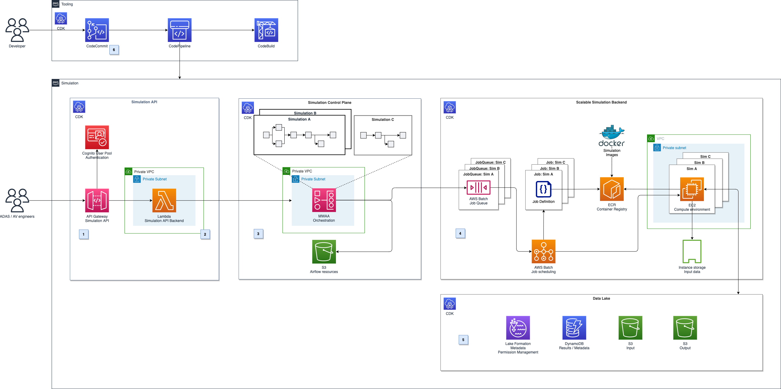
To migrate to AWS, install the AWS MGN Replication Agent on your source servers and define replication settings in the AWS MGN console, shown in Figure 1. Replication servers receive data from an agent running on source servers, and write this data to the Amazon Elastic Block Store (EBS) volumes. Your replicated data is compressed and encrypted in transit and at rest using EBS encryption.
AWS MGN keeps your source servers up to date on AWS using nearly continuous, block-level data replication. It uses your defined launch settings to launch instances when you conduct non-disruptive tests or perform a cutover. After confirming that your launched instances are operating properly on AWS, you can decommission your source servers.
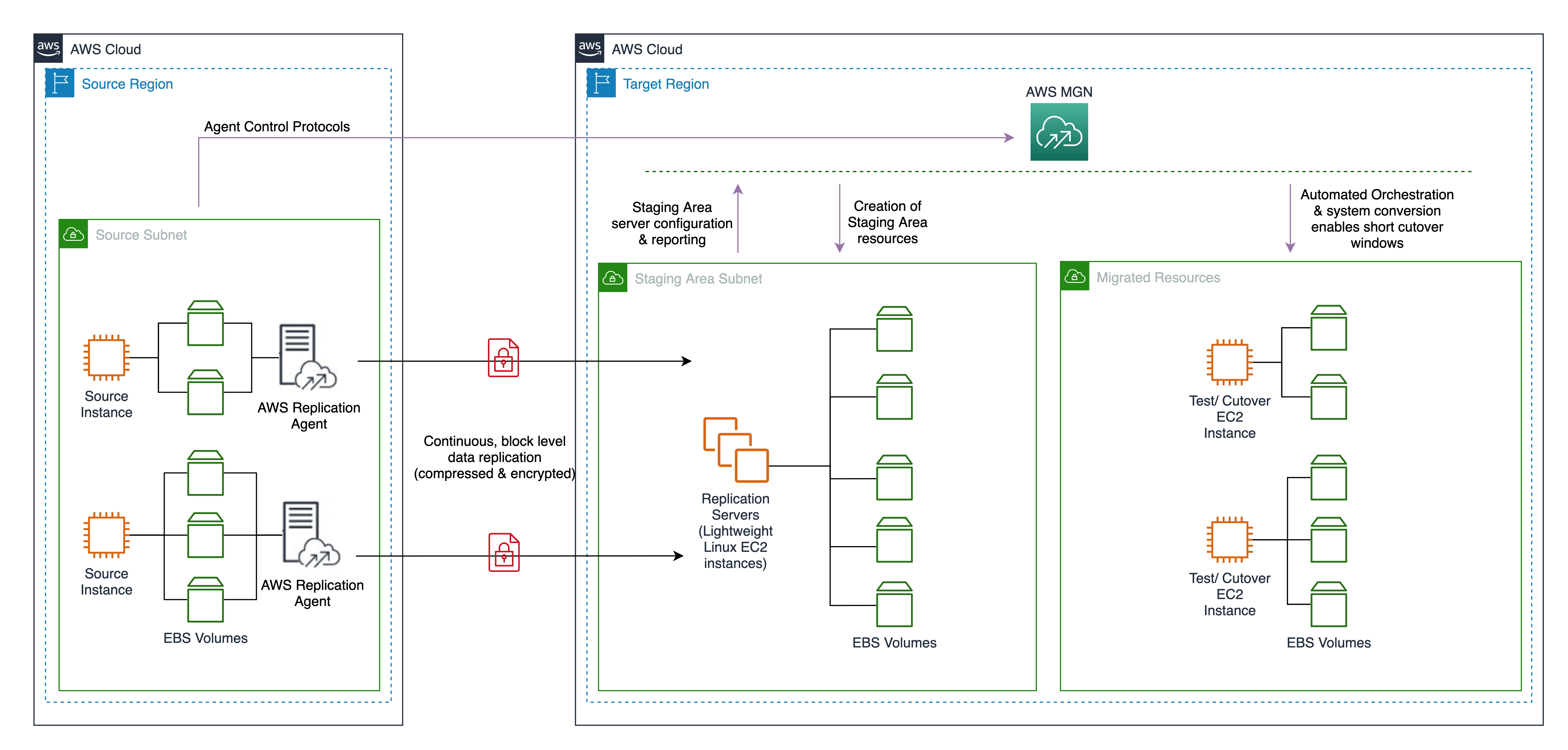
Figure 1. MGN service architecture
Steps for migration with AWS MGN
This tutorial assumes that you already have your source AWS Region set up with Amazon EC2-hosted workloads running and a target AWS Region defined.
Migrating Amazon EC2 workload across AWS Regions include the following steps:
- Create the Replication Settings template. These settings are used to create and manage your staging area subnet with lightweight Amazon EC2 instances. These instances act as replication servers used to replicate data between your source servers and AWS.
- Install the AWS Replication Agent on your source instances to add them to the AWS MGN console.
- Configure the launch settings for each source server. These are a set of instructions that determine how a Test or Cutover instance will be launched for each source server on AWS.
- Initiate the test/cutover to the target Region.
Prerequisites
Following are the prerequisites:
- AWS Identity and Access Management (IAM) user with required credentials, as defined in the AWS MGN documentation
- A staging area subnet created in the target Region, as defined in the AWS MGN documentation
- A VPC and subnet in the target Region where target instances will be launched
- Security groups that will be attached to migrated instances
- Network preparations in both Regions as defined in the AWS MGN documentation
Setting up AWS MGN for multi-Region migration
This section will guide you through AWS MGN configuration setup for multi-Region migration.
Log into your AWS account, select the target AWS Region, and complete the prerequisites. Then you are ready to configure AWS MGN:
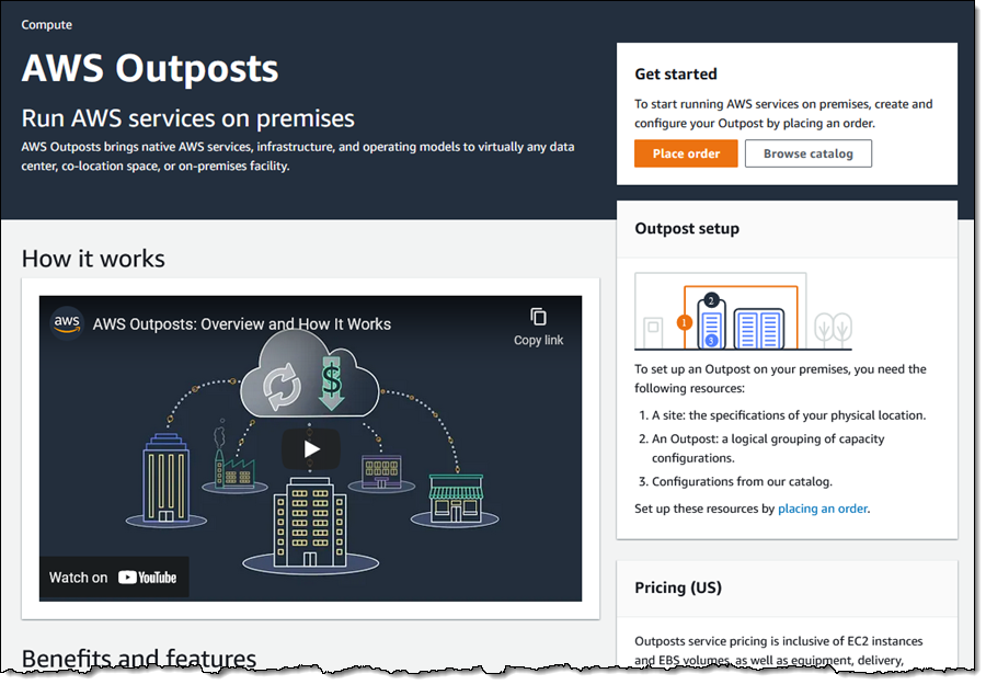
1. Choose Get started on the AWS MGN landing page.
2. Create the Replication Settings template (see Figure 2):
- Select Staging area subnet for Replication Server
- Choose Replication Server instance type (By default, AWS MGN uses t3.small instance type)
- Choose default or custom Amazon EBS encryption
- Enable ‘Always use the Application Migration Service security group’
- Add custom Replication resources tags
- Select Create Template button
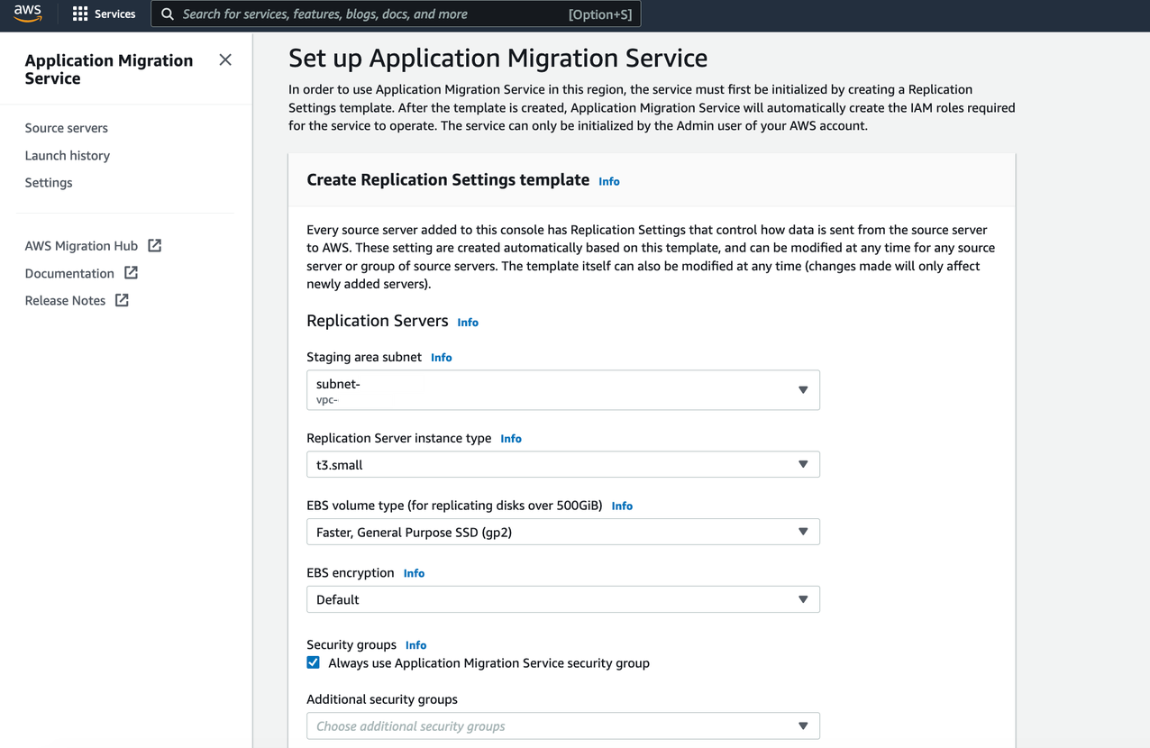
Figure 2. Replication Settings template creation
3. Add source servers to AWS MGN:
- Select Add Servers following Source Servers (AWS MGN > Source Servers)
- Enter OS, Replication Preferences, IAM Access Key and Secret Access Key ID of the IAM user created following Prerequisites. This does not expose your Secret Access Key ID in any request
- Copy the installation command and run on your source server for agent installation
After successful agent installation, the source server is listed on the Source Servers page. Data replication begins after completion of the Initial Sync steps.
4. Monitor the Initial Sync status (shown in Figure 3):
- Source server name > Migration Dashboard > Data Replication Status
(Refer to the Source Servers page documentation for more details) - After 100% initial data replication confirm:
- Migration Lifecycle = Ready for testing
- Next step = Launch test instance
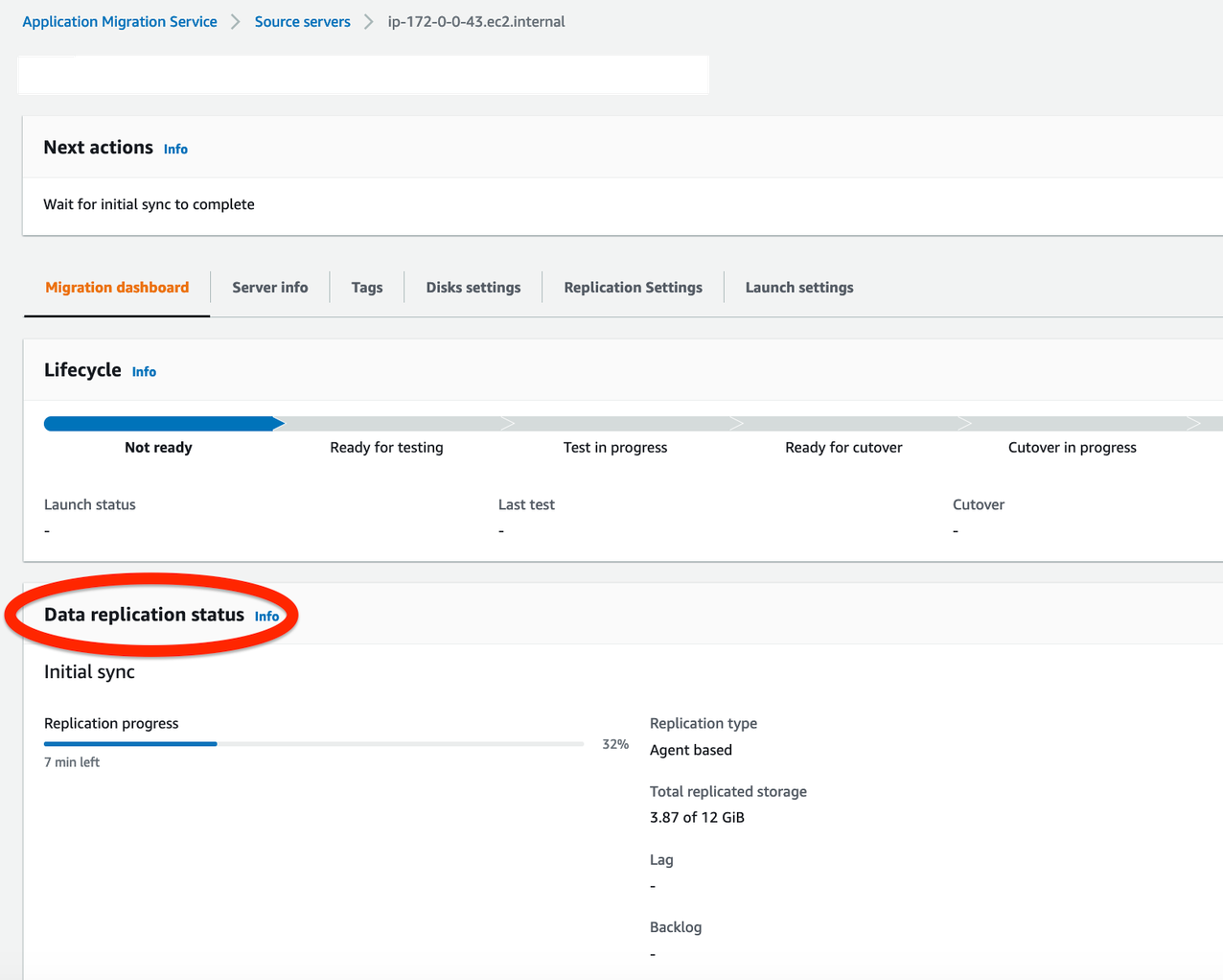
Figure 3. Monitoring initial replication status
5. Configure Launch Settings for each server:
- Source servers page > Select source server
- Navigate to the Launch settings tab (see Figure 4.) For this tutorial we won’t adjust the General launch settings. We will modify the EC2 Launch Template instead
- Click on EC2 Launch Template > About modifying EC2 Launch Templates > Modify
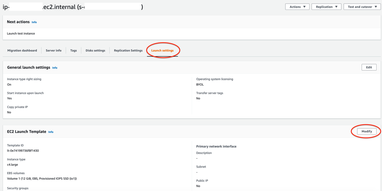
Figure 4. Modifying EC2 Launch Template
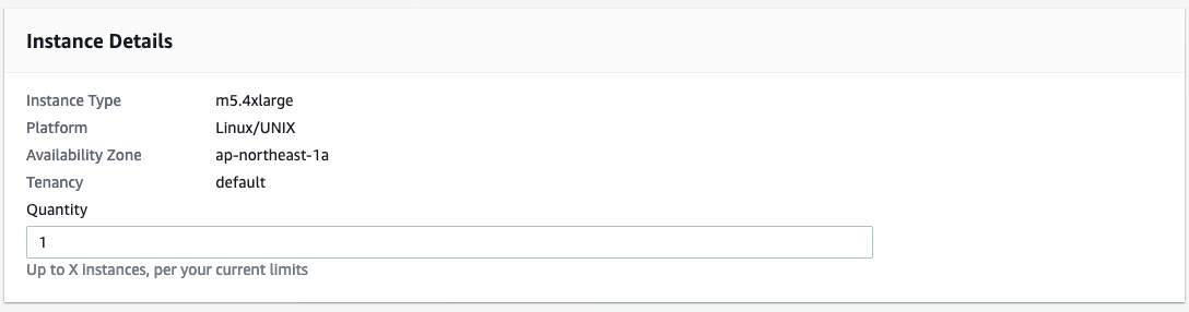
6. Provide values for Launch Template:
- AMI: Recents tab > Don’t include in launch template
- Instance Type: Can be kept same as source server or changed as per expected workload
- Key pair (login): Create new or use existing if already created in the Target AWS Region
- Network Settings > Subnet: Subnet for launching Test instance
- Advanced network configuration:
- Security Groups: For access to the test and final cutover instances
- Configure Storage: Size – Do not change or edit this field
- Volume type: Select any volume type (io1 is default)
- Review details and click Create Template Version under the Summary section on right side of the console
7. Every time you modify the Launch template, a new version is created. Set the launch template that you want to use with MGN as the default (shown in Figure 5):
- Navigate to Amazon EC2 dashboard > Launch Templates page
- Select the Launch template ID
- Open the Actions menu and choose Set default version and select the latest Launch template created
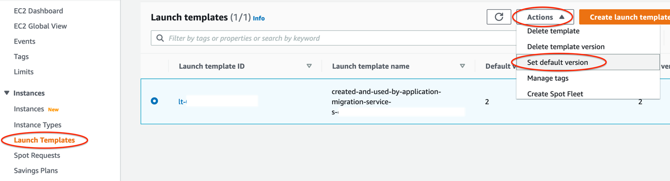
Figure 5. Setting up your Launch template as the default
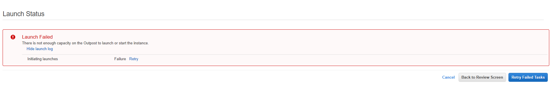
8. Launch a test instance and perform a Test prior to Cutover to identify potential problems and solve them before the actual Cutover takes place:
- Go to the Source Servers page (see Figure 6)
- Select source server > Open Test and Cutover menu
- Under Testing, choose Launch test instances
- Launch test instances for X servers > Launch
- Choose View job details on the ‘Launch Job Created’ dialog box to view the specific Job details for the test launch in the Launch History tab
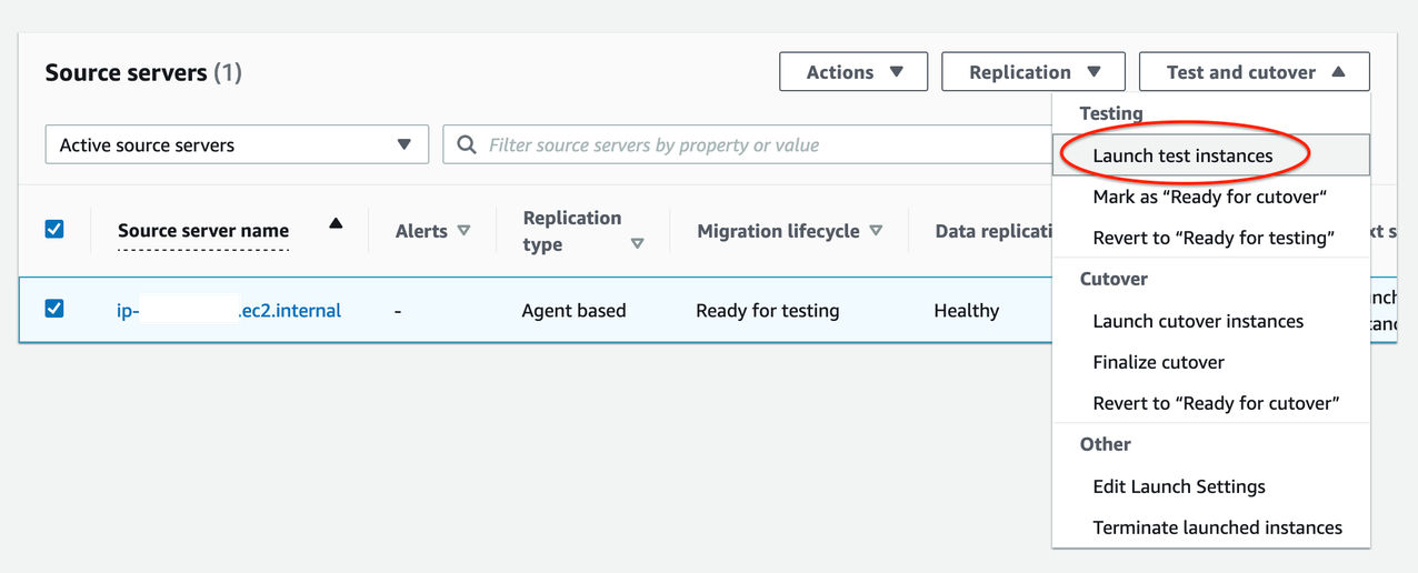
Figure 6. Launching test instances
9. Validate launch of test instance (shown in Figure 7) by confirming:
- Alerts column = Launched
- Migration lifecycle column = Test in progress
- Next step column = Complete testing and mark as ‘Ready for cutover’
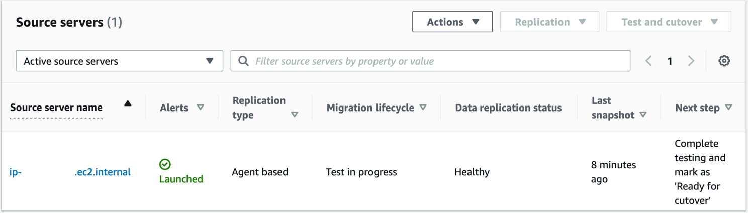
Figure 7. Validating launch of test instances
10. SSH/ RDP into Test instance (view from EC2 console) and validate connectivity. Perform acceptance tests for your application as required. Revert the test if you encounter any issues.
11. Terminate Test instances after successful testing:
- Go to Source servers page
- Select source server > Open Test and Cutover menu
- Under Testing, choose Mark as “Ready for cutover”
- Mark X servers as “Ready for cutover” > Yes, terminate launched instances (recommended) > Continue
12. Validate the status of termination job and cutover readiness:
- Migration Lifecycle = Ready for cutover
- Next step = Launch cutover instance
13. Perform the final cutover at a set date and time:
- Go to Source servers page (see Figure 8)
- Select source server > Open Test and Cutover menu
- Under Cutover, choose Launch cutover instances
- Launch cutover instances for X > Launch
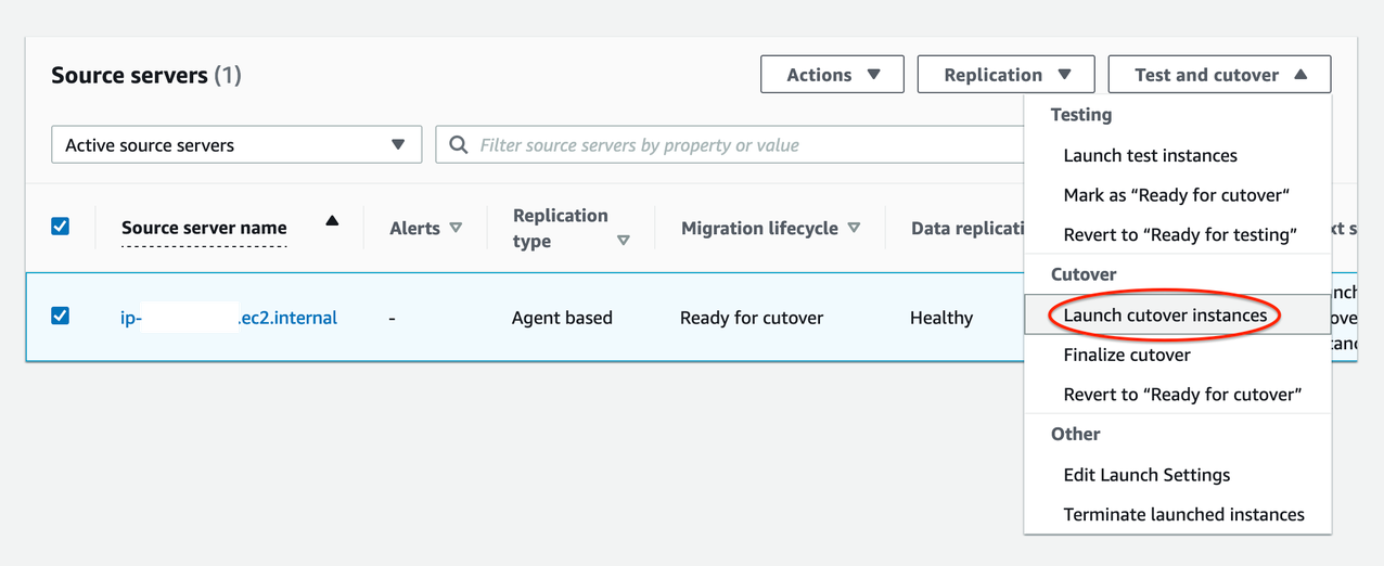
Figure 8. Performing final Cutover by launching Cutover instances
14. Monitor the indicators to validate the success of the launch of your Cutover instance (shown in Figure 9):
- Alerts column = Launched
- Migration lifecycle column = Cutover in progress
- Data replication status = Healthy
- Next step column = Finalize cutover
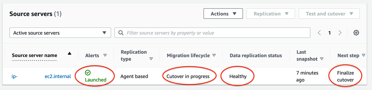
Figure 9. Indicators for successful launch of Cutover instances
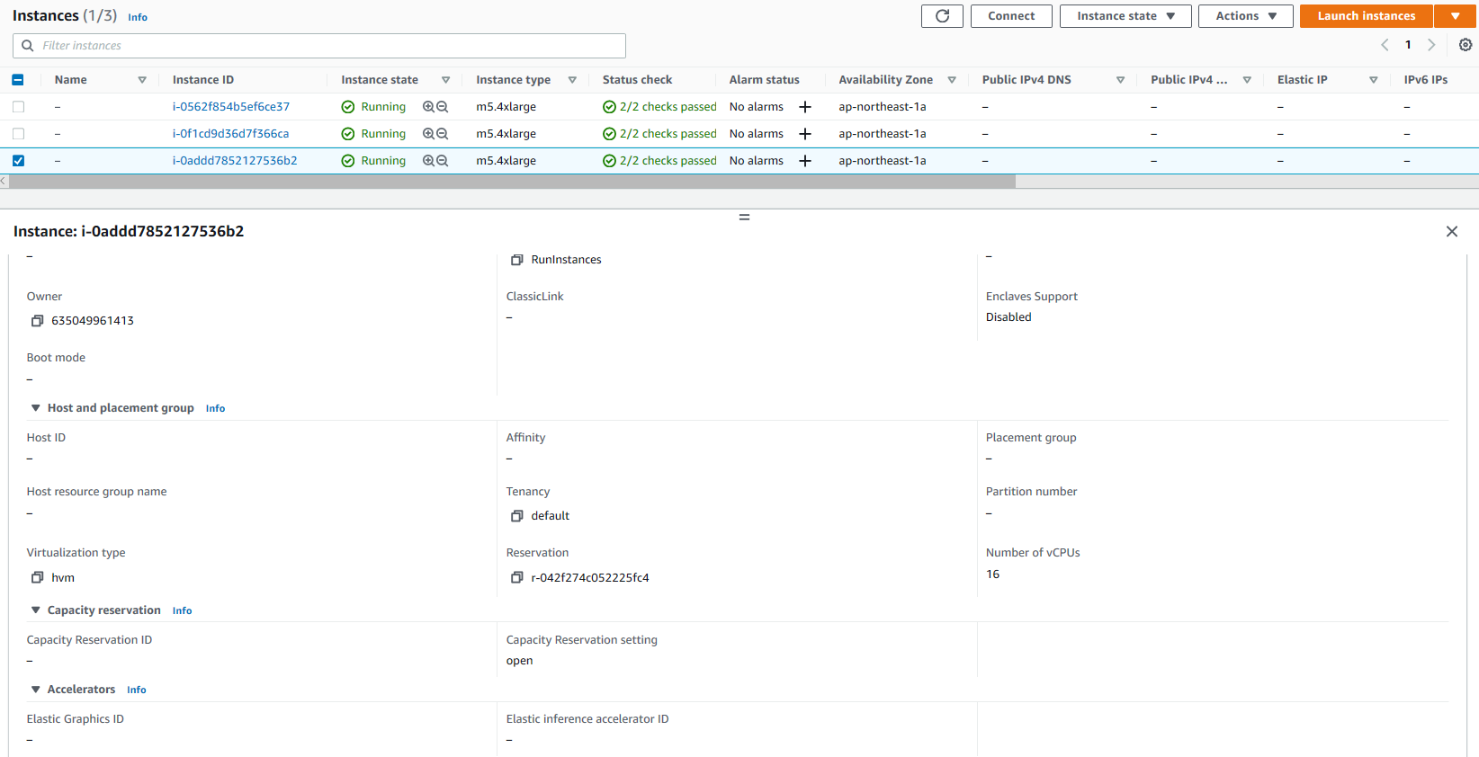
15. Test Cutover Instance:
- Navigate to Amazon EC2 console > Instances (running)
- Select Cutover instance
- SSH/ RDP into your Cutover instance to confirm that it functions correctly
- Validate connectivity and perform acceptance tests for your application
- Revert Cutover if any issues
16. Finalize the cutover after successful validation:
- Navigate to AWS MGN console > Source servers page
- Select source server > Open Test and Cutover menu
- Under Cutover, choose Finalize Cutover
- Finalize cutover for X servers > Finalize
17. At this point, if your cutover is successful:
- Migration lifecycle column = Cutover complete,
- Data replication status column = Disconnected
- Next step column = Mark as archived
The cutover is now complete and that the migration has been performed successfully. Data replication has also stopped and all replicated data will now be discarded.
Cleaning up
Archive your source servers that have launched Cutover instances to clean up your Source Servers page-
- Navigate to Source Servers page (see Figure 10)
- Select source server > Open Actions
- Choose Mark as archived
- Archive X server > Archive
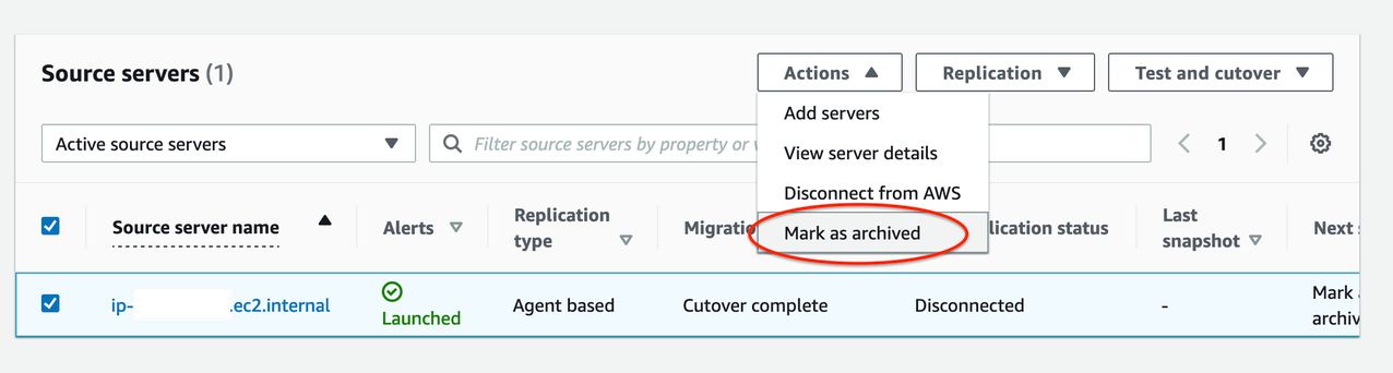
Figure 10. Mark source servers as archived that are cutover
Conclusion
In this post, we demonstrated how AWS MGN simplifies, expedites, and reduces the cost of migrating Amazon EC2-hosted workloads from one AWS Region to another. It integrates with AWS Migration Hub, enabling you to organize your servers into applications. You can track the progress of all your MGN at the server and app level, even as you move servers into multiple AWS Regions. Choose a Migration Hub Home Region for MGN to work with the Migration Hub.
Here are the AWS MGN supported AWS Regions. If your preferred AWS Region isn’t currently supported or you cannot install agents on your source servers, consider using CloudEndure Migration or AWS Server Migration Service respectively. CloudEndure Migration will be discontinued in all AWS Regions on December 30, 2022. Refer to CloudEndure Migration EOL for more information.
Note: Use of AWS MGN is free for 90 days but you will incur charges for any AWS infrastructure that is provisioned during migration and after cutover. For more information, refer to the pricing page.
Thanks for reading this blog post! If you have any comments or questions, feel free to put them in the comments section.


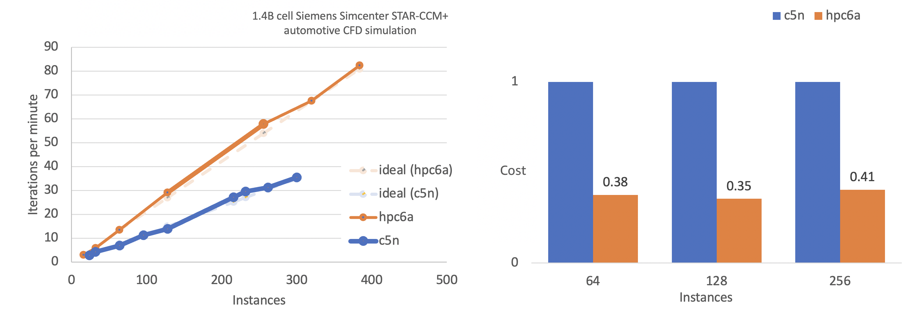
 processor (Milan) cores with 384 GB RAM, and offers up to 65 percent better price-performance over comparable x86-based compute-optimized instances.