Edge computing comprises elements of geography and networking and brings computing closer to the end users of the application.
For example, using a content delivery network (CDN) such as AWS CloudFront can help video streaming providers reduce latency for distributing their material by taking advantage of caching at the edge. Another example might look like an Internet of Things (IoT) solution that helps a company run business logic in remote areas or with low latency.
IoT is a challenging field because there are multiple aspects to consider as architects, like hardware, protocols, networking, and software. All of these aspects must be designed to interact together and be fault tolerant.
In this edition of Let’s Architect!, we share resources that are helpful for teams that are approaching or expanding their workloads for edge computing We cover macro topics such as security, best practices for IoT, patterns for machine learning (ML), and scenarios with strict latency requirements.
In Let’s Architect! Architecting for Machine Learning, we touched on some of the most relevant aspects to consider while putting ML into production. However, in many scenarios, you may also have specific constraints like latency or a lack of connectivity that require you to design a deployment at the edge.
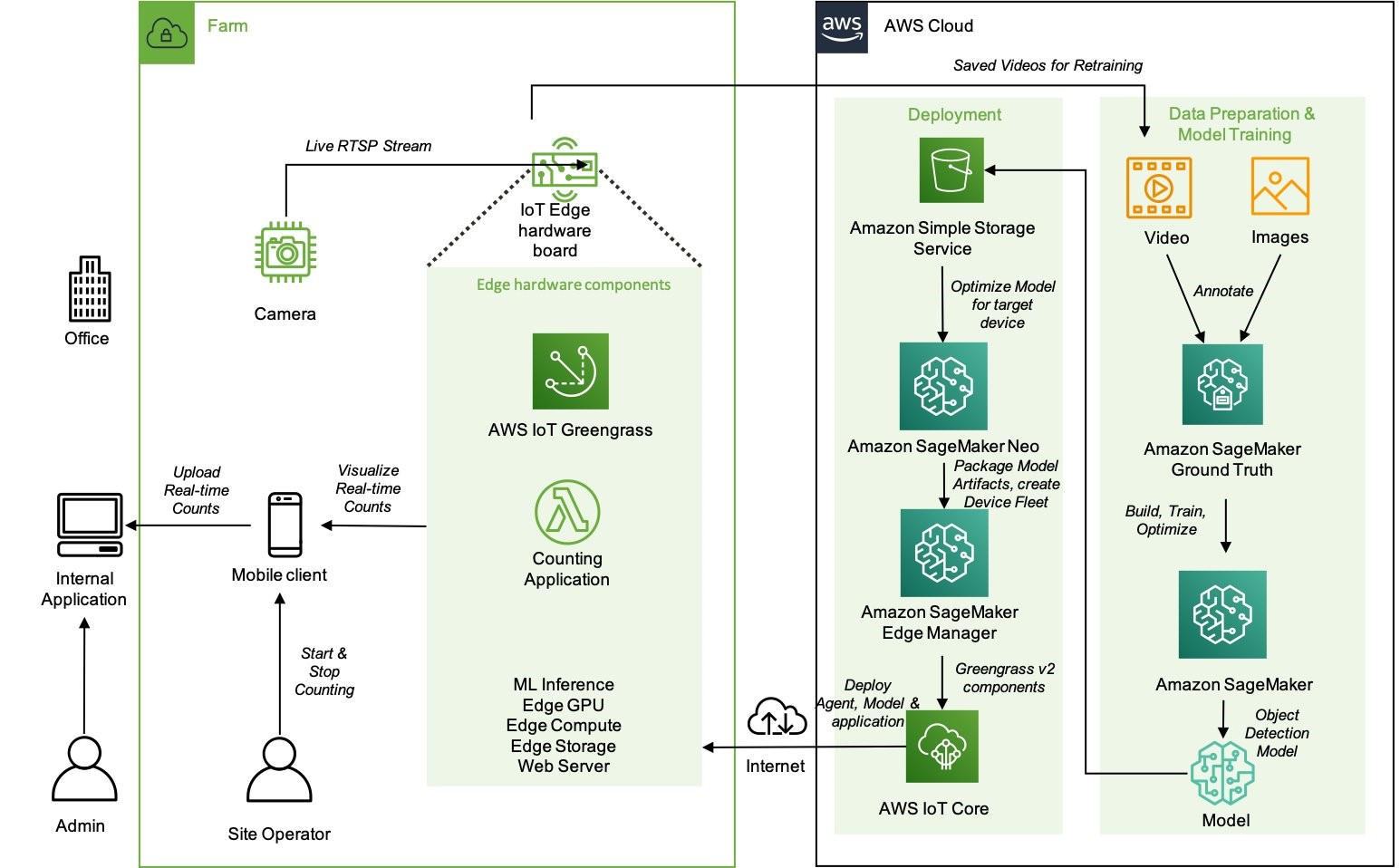
This blog post considers a solution based on ML applied to agriculture, where a reliable connection to the Internet is not always available. You can learn from this scenario, which includes information from model training to deployment, to design your ML workflows for the edge. The solution uses Amazon SageMaker in the cloud to explore, train, package, and deploy the model to AWS IoT Greengrass, which is used for inference at the edge.
High-level architecture of the components that reside on the farm and how they interact with the cloud environment
Security is one of the fundamental pillars described in the AWS Well-Architected Framework. In all organizations, security is a major concern both for the business and the technical stakeholders. It impacts the products they are building and the perception that customers have.
We covered security in Let’s Architect! Architecting for Security, but we didn’t focus specifically on edge technologies. This whitepaper shows approaches for implementing a security strategy at the edge, with a focus on describing how AWS services can be used. You can learn how to secure workloads designed for content delivery, as well as how to implement network protection to defend against DDoS attacks and protect your IoT solutions.
The AWS Well-Architected Tool is designed to help you review the state of your applications and workloads. It provides a central place for architectural best practices and guidance
AWS Outposts allows companies to run some AWS services on-premises, which may be crucial to comply with strict data residency or low latency requirements. With Outposts, you can deploy servers and racks from AWS directly into your data center.
This whitepaper introduces architectural patterns, anti-patterns, and recommended practices for building highly available systems based on Outposts. You will learn how to manage your Outposts capacity and use networking and data center facility services to set up highly available solutions. Moreover, you can learn from mental models that AWS engineers adopted to consider the different failure modes and the corresponding mitigations, and apply the same models to your architectural challenges.
An Outpost deployed in a customer data center and connected back to its anchor Availability Zone and parent Region
The AWS Well-Architected Lenses are designed for specific industry or technology scenarios. When approaching the IoT domain, the AWS IoT Lens is a key resource to learn the best practices to adopt for IoT. This whitepaper breaks down the IoT workloads into the different subdomains (for example, communication, ingestion) and maps the AWS services for IoT with each specific challenge in the corresponding subdomain.
As architects and developers, we tend to automate and reduce the risk of human errors, so the IoT Lens Checklist is a great resource to review your workloads by following a structured approach.
Workload context checklist from the IoT Lens Checklist
See you next time!
Thanks for joining our discussion on architecting for the edge! See you in two weeks when we talk about database architectures on AWS.
Packet captures are a critical tool used by network and security engineers every day. As more network functions migrate from legacy on-prem hardware to cloud-native services, teams risk losing the visibility they used to get by capturing 100% of traffic funneled through a single device in a datacenter rack. We know having easy access to packet captures across all your network traffic is important for troubleshooting problems and deeply understanding traffic patterns, so today, we’re excited to announce the general availability of on-demand packet captures from Cloudflare’s global network.
What are packet captures and how are they used?
A packet capture is a file that contains all packets that were seen by a particular network box, usually a firewall or router, during a specific time frame. Packet captures are a powerful and commonly used tool for debugging network issues or getting better visibility into attack traffic to tighten security (e.g. by adding firewall rules to block a specific attack pattern).
A network engineer might use a pcap file in combination with other tools, like mtr, to troubleshoot problems with reachability to their network. For example, if an end user reports intermittent connectivity to a specific application, an engineer can set up a packet capture filtered to the user’s source IP address to record all packets received from their device. They can then analyze that packet capture and compare it to other sources of information (e.g. pcaps from the end user’s side of the network path, traffic logs and analytics) to understand the magnitude and isolate the source of the problem.
Security engineers can also use packet captures to gain a better understanding of potentially malicious traffic. Let’s say an engineer notices an unexpected spike in traffic that they suspect could be an attempted attack. They can grab a packet capture to record the traffic as it’s hitting their network and analyze it to determine whether the packets are valid. If they’re not, for example, if the packet payload is randomly generated gibberish, the security engineer can create a firewall rule to block traffic that looks like this from entering their network.
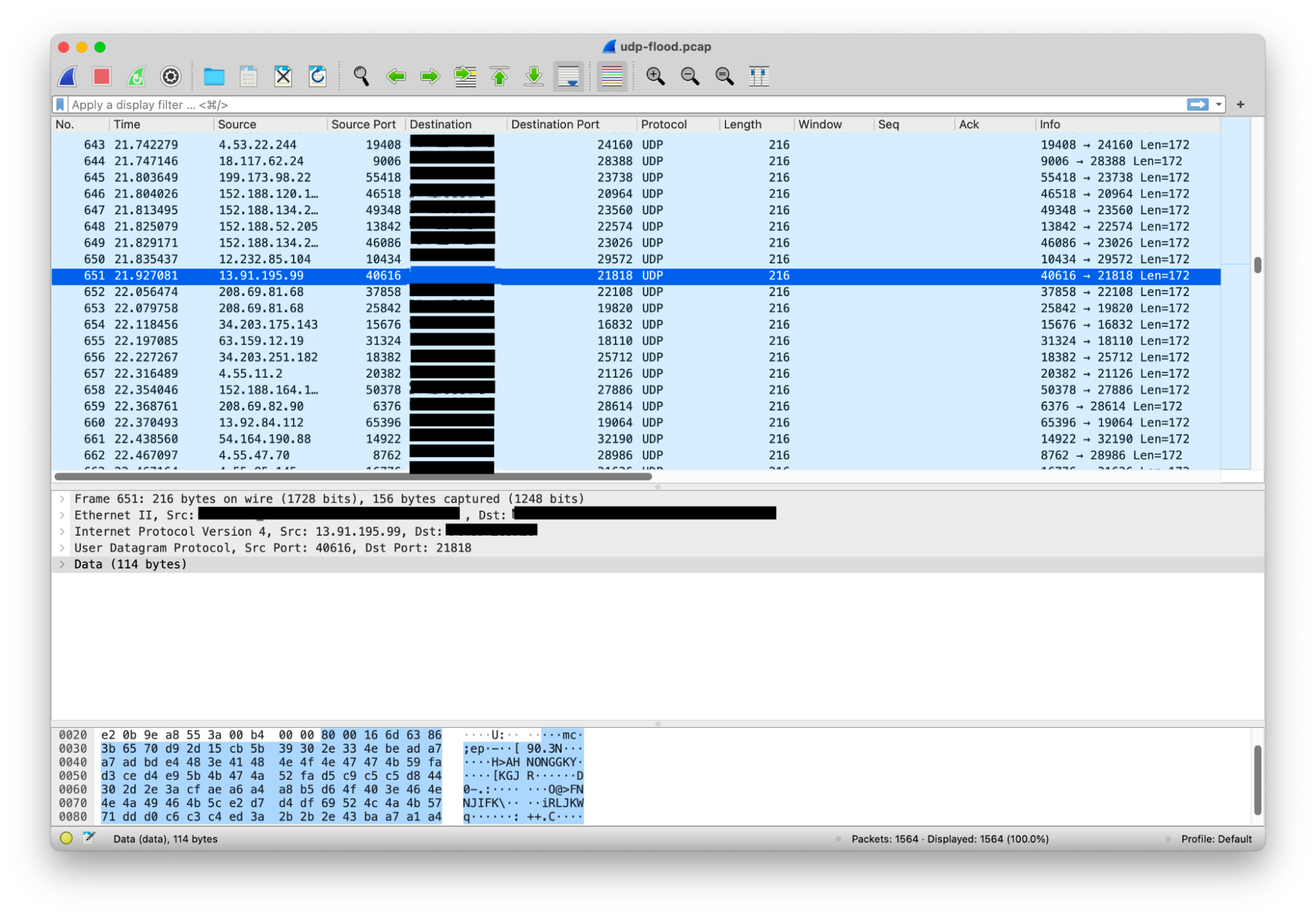
Example of a packet capture from a recent DDoS attack targeted at Cloudflare infrastructure. The contents of this pcap can be used to create a “signature” to block the attack.
Fragmenting traffic creates gaps in visibility
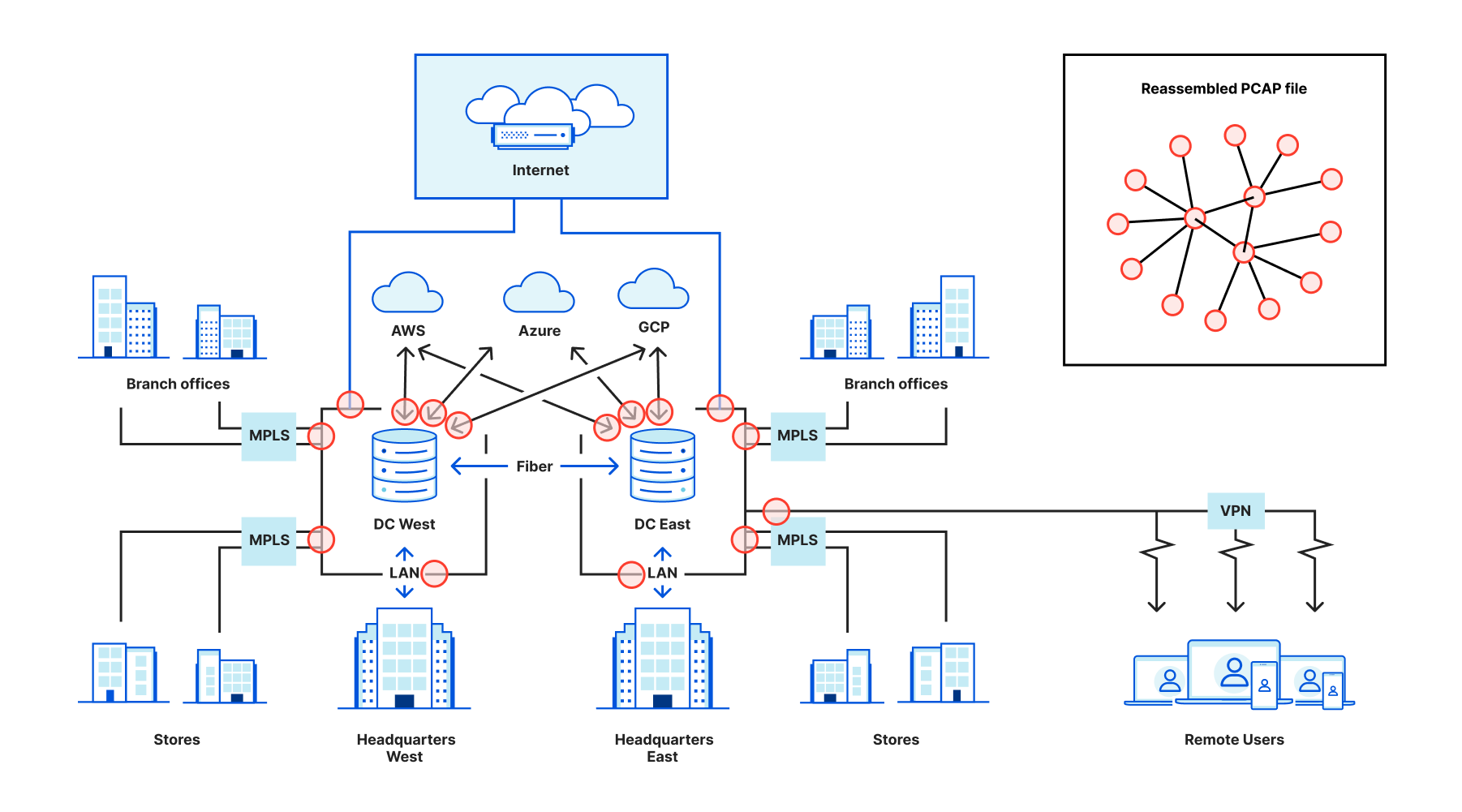
Traditionally, users capture packets by logging into their router or firewall and starting a process like tcpdump. They’d set up a filter to only match on certain packets and grab the file. But as networks have become more fragmented and users are moving security functions out to the edge, it’s become increasingly challenging to collect packet captures for relevant traffic. Instead of just one device that all traffic flows through (think of a drawbridge in the “castle and moat” analogy) engineers may have to capture packets across many different physical and virtual devices spread across locations. Many of these packets may not allow taking pcaps at all, and then users have to try to stitch them back together to create a full picture of their network traffic. This is a nearly impossible task today and only getting harder as networks become more fractured and complex.
On-demand packet captures from the Cloudflare global network
With Cloudflare, you can regain this visibility. With Magic Transit and Magic WAN, customers route all their public and private IP traffic through Cloudflare’s network to make it more secure, faster, and more reliable, but also to increase visibility. You can think of Cloudflare like a giant, globally distributed version of the drawbridge in our old analogy: because we act as a single cloud-based router and firewall across all your traffic, we can capture packets across your entire network and deliver them back to you in one place.
How does it work?
Customers can request a packet capture using our Packet Captures API. To get the packets you’re looking for you can provide a filter with the IP address, ports, and protocol of the packets you want.
Example of a request for packet capture using our API.
We leverage nftables to apply the filter to the customer’s incoming packets and log them using nflog:
table inet pcaps_1 {
    chain pcap_1 {
        ip protocol 6 ip saddr 1.2.3.4 log group 1 comment “packet capture”
    }
}
Example nftables configuration used to filter log customer packets
nflog creates a netfilter socket through which logs of a packet are sent from the Linux kernel to user space. In user space, we use tcpdump to read packets off the netfilter socket and generate a packet capture file:
tcpdump -i nflog:1 -w pcap_1.pcap
Example tcpdump command to create a packet capture file.
Usually tcpdump is used by listening to incoming packets on a network interface, but in our case we configure it to read packet logs from an nflog group. tcpdump will convert the packet logs into a packet capture file.
Once we have a packet capture file, we need to deliver it to customers. Because packet capture files can be large and contain sensitive information (e.g. packet payloads), we send them to customers directly from our machines to a cloud storage service of their choice. This means we never store sensitive data, and it’s easy for customers to manage and store these large files.
Get started today
On-demand packet captures are now generally available for customers who have purchased the Advanced features of Magic Firewall. The packet capture API allows customers to capture the first 160 bytes of packets, sampled at a default rate of 1/100. More functionality including full packet captures and on-demand packet capture control in the Cloudflare Dashboard is coming in the following weeks. Contact your account team to stay updated on the latest!
In 2020, we launched AWS IoT Greengrass 2.0, an open-source edge runtime and cloud service for building, deploying, and managing device software and applications. Today, we’re very excited to announce the ability to securely manage your AWS IoT Greengrass edge devices using AWS Systems Manager (SSM).
Managing vast fleets of varying systems and applications remotely can be a challenge for administrators of edge devices. AWS IoT Greengrass was built to enable these administrators to manage their edge device application stack. While this addressed the needs of many typical edge device administrators, system software on these devices still needed to be updated and maintained through operational policies consistent with those of their broader IT organizations. To this end, administrators would typically have to build or integrate tools to create a centralized interface for managing their edge and IT device software stacks – from security updates, to remote access, and operating system patches.
Until today, IT administrators have had to build or integrate custom tools to make sure edge devices can be managed alongside EC2 and on-prem instances, through a consistent set of policies. At scale, managing device and systems software across a wide variety of edge and IT systems becomes a significant investment in time and money. This is time that could be better spent deploying, optimizing, and managing the very edge devices that they’re maintaining.
What’s New? Today, we have integrated IoT Greengrass and Systems Manager to simplify the management and maintenance of system software for edge devices. When coupled with the AWS IoT Greengrass Client Software, edge device administrators now can remotely access and securely manage with the multitude of devices that they own – from OS patching, to application deployments. Additionally, regularly scheduled operations that maintain edge compute systems can be automated, all without the need for creating additional custom processes. For IT administrators, this release gives a complete overview of all of their devices through a centralized interface, and a consistent set of tools and policies with the AWS Systems Manager.
For customers new to the AWS IoT Greengrass platform, the integration with Systems Manager simplifies setup even further with a new on- boarding wizard that can reduce the time it takes to create operational management systems for edge devices from weeks to hours.
How is this achieved? This new capability is enabled by the AWS Systems Manager (SSM) Agent. As of today, customers can deploy the AWS Systems Manager Agent, via the AWS IoT Greengrass console, to their existing edge devices. Once installed on each device, AWS Systems Manager will list all of the devices in the Systems Manager Console, thereby giving administrators and IoT stakeholders an overview of their entire fleet. When coupled with the AWS IoT Greengrass console, administrators can manage their newly configured devices remotely; patching or updating operating systems, troubleshooting remotely, and deploying new applications, all through a centralized, integrated user interface. Devices can be patched individually, or in groups organized by tags or resource groups.
Further information These new features are now available in all regions where AWS Systems Manager and AWS IoT Greengrass are available. To get started, please visit the IoT Greengrass home page.
Today, the AWS Panorama Appliance is generally available to all of you. The AWS Panorama Appliance is a computer vision (CV) appliance designed to be deployed on your network to analyze images provided by your on-premises cameras.
Every week, I read about new and innovative use cases for computer vision. Some customers are using CV to verify pallet trucks are parked in designated areas to ensure worker safety in warehouses, some are analyzing customer walking flows in retail stores to optimize space and product placement, and some are using it to recognize cats and mice, just to name a few.
AWS customers agree the cloud is the most convenient place to train computer vision models thanks to its virtually infinite access to storage and compute resources. In the cloud, data scientists have access to powerful tools such as Amazon SageMaker and a wide variety of compute resources and frameworks.
However, when it’s time to analyze images from one or multiple video feeds, many of you are telling us the cloud is not the place where you want to run such workloads. There are a number of reasons for that: sometimes the facilities where the images are captured do not have enough bandwidth to send video feeds to the cloud, some use cases require very low latency, or some just want to keep their images on premises and not send them for analysis outside of their network.
AWS Panorama is a machine learning appliance and software development kit (SDK) that allows you to bring computer vision to on-premises cameras to make predictions locally with high accuracy and low latency. With the AWS Panorama Appliance, you can automate tasks that have traditionally required human inspection to improve visibility into potential issues. For example, you can use AWS Panorama Appliance to evaluate manufacturing quality, identify bottlenecks in industrial processes, and monitor workplace security even in environments with limited or no internet connectivity. The software development kit allows camera manufacturers to bring equivalent capabilities directly inside their IP camera.
As usual on this blog, I would like to walk you through the development and deployment of a computer vision application for the AWS Panorama Appliance. The demo application from this blog uses a machine learning model to recognise objects in frames of video from a network camera. The application loads a model onto the AWS Panorama Appliance, gets images from a camera, and runs those images through the model. The application then overlays the results on top of the original video and outputs it to a connected display. The application uses libraries provided by AWS Panorama to interact with input and output video streams and the model, no low level programming is required.
Concepts The AWS Panorama Appliance is the hardware that runs your applications. You use the AWS Panorama console or AWS SDKs to register an appliance, update its software, and deploy applications to it. The software that runs on the appliance discovers and connects to camera streams, sends frames of video to your application, and optionally displays video output on an attached display.
The appliance is an edge device. Instead of sending images to the AWS Cloud for processing, it runs applications locally on optimized hardware. This enables you to analyze video in real time and process the results with limited connectivity. The appliance only requires an internet connection to report its status, upload logs, and get software updates and deployments.
An application comprises multiple components called nodes, which represent cameras, models, code, or global variables. A node can be configuration only (inputs and outputs), or include artifacts (models and code). Application nodes are bundled in node packages that you upload to an S3 access point, where the AWS Panorama Appliance can access them. An application manifest is a configuration file that defines connections between the nodes.
A computer vision model is a machine learning network that is trained to process images. Computer vision models can perform various tasks such as classification, detection, segmentation, and tracking. A computer vision model takes an image as input and outputs information about the image or objects in the image.
Now that we grasp the concepts, let’s get our hands on.
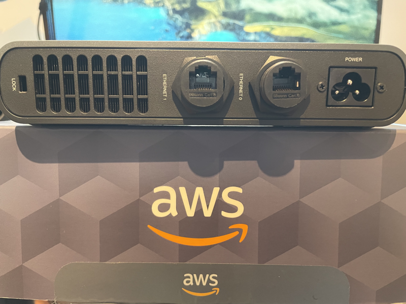
Unboxing Your AWS Panorama Appliance In the box the service team sent me, I found the appliance itself (no surprise!), a power cord and two ethernet cables. The box also contains a USB key to initially configure the appliance. The device is designed to work in industrial environments. It has two ethernet ports next to the power connector on the back. On the front, protected behind a sliding door, I found a SD card reader, one HDMI connector and two USB ports. There is also a power button and a reset button to reinitialise the device to its factory state.
Configuring Your Appliance I first configured it for my network (cable + DHCP, but it also supports static IP configuration) and registered it to securely connect back to my AWS Account. To do so, I navigated to the AWS Management Console, entered my network configuration details. It generated a set of configuration files and certificates. I copied them to the appliance using the provided USB key. My colleague Martin Beeby shared screenshots of this process. The team slightly modified the screens based on the feedback they received during the preview, but I don’t think it is worth going through the step-by-step process again. Tip from the field: be sure to use the USB key provided in the box, it is correctly formatted and automatically recognised by the appliance (my own USB key was not recognized properly).
When receiving an application developed by someone else, like the sample application, I have to replace AWS account IDs in all application files and directory names. I do this with one single command:
panorama-cli import-application
Application Structure A Panorama application structure looks as follows:
graph.json lists all the packages and nodes in this application. Nodes are the way to define an application in Panorama.
in each package package.json has details about the package and the assets it uses.
model package model has a descriptor.json which contains the metadata required for compiling the model.
container packagesample-app package contains the application code in the src directory and a Dockerfile to build the container. descriptor.json has details about which command and file to use when the container is launched.
assets directory is where all the assets reside, such as packaged code and compiled models. You should not make any changes in this directory.
Note that package names are prefixed with your account number.
A Note About the Cameras AWS Panorama Appliance has a concept of “abstract cameras”. Abstract camera sources are placeholders that can be mapped to actual camera devices during application deployment. The Test Utility for Panorama allows you to map abstract cameras to video files for easy, repeatable tests.
Adding a ML Model The AWS Panorama Appliance supports multiple ML Model frameworks. Models may be trained on Amazon SageMaker or any other solution of your choice. I downloaded my ML model from S3 and import it to my project:
Behind the scenes, ML Models are compiled to optimise them to the Nvidia Accelerated Linux Arm64 architecture of the AWS Panorama Appliance.
Package the Application Now that I have a ML model and my application code packaged in a container, I am ready to package my application assets for AWS Panorama Appliance:
panorama-cli package-application
This command uploads all my application assets to the AWS cloud account along with all the manifests.
Deploy the Application Finally I deploy the application to the AWS Panorama Appliance. A deployment copies the application and its configuration, like camera stream selection, from the AWS cloud to my on-premise AWS Panorama Appliance. I may deploy my application programmatically using Python code (and the Boto3 SDK you might know already):
client = boto3.client('panorama')
client.create_application_instance(
    Name="AWS News Blog Sample Application",
    Description="An object detection app",
    ManifestPayload={
       'PayloadData': manifest         # <== this is the graph.json file content
    },
    RuntimeRoleArn=role,               # <== this is a role that gives my app permissions to use AWS Services such as Cloudwatch
    DefaultRuntimeContextDevice=device # <== this is my device name
)
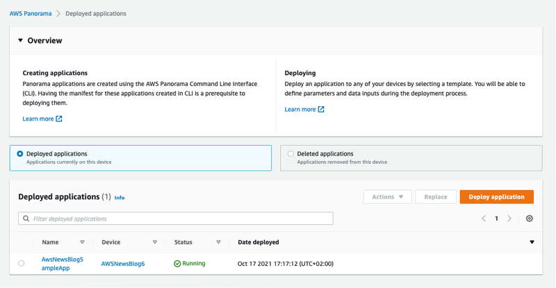
On Deployed applications, I select Deploy application.
I copy and paste the content of graphs/<project name>/graph.json to the console and select Next.
I give my application a name and an optional description. I select Proceed to deploy.
The next steps are
declare an IAM role to give permissions to my application to use AWS Service. The minimal permissions set allows to call the PuMetricData API on CloudWatch.
select the AWS Panorama Appliance I want to deploy to
map the abstract cameras defined in the application descriptors.json to physical cameras known by the AWS Panorama Appliance
fill in any application-specific inputs, such as acceptable threshold value, log level etc.
The deployment takes 15-30 minutes depending on the size of your code and your ML models, and the appliance available bandwidth. Eventually, the status turn green to “Running”.
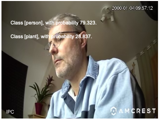
Once the application is deployed to your AWS Panorama Appliance it begins to run, continuously analyzing video and generating highly accurate predictions locally within milliseconds. I connect an HDMI cable to the AWS Panorama Appliance to monitor the output, and I can see:
Should anything goes wrong during the deployment or during the life of the application, I have access to the logs on Amazon CloudWatch. There are two log streams created, one for the AWS Panorama Appliance itself and one for the application.
Pricing and Availability The AWS Panorama Appliance is available to purchase at AWS Elemental order page in the AWS Console. You can place orders from the United States, Canada, the United Kingdom, and the European Union. There is a one-time charge of $4,000 for the appliance itself.
There is a usage charge of $8.33 / month / camera feed.
AWS Panorama stores versioned copies of all assets deployed to the AWS Panorama Appliance (including ML models and business logic) in the cloud. You are charged $0.10 per-GB, per-month for this storage.
You may incur additional charges if the business logic deployed to your AWS Panorama Appliance uses other AWS services. For example, if your business logic uploads ML predictions to S3 for offline analysis, you will be billed separately by S3 for any storage charges incurred.
The AWS Panorama Appliance can be installed anywhere. The appliance connects back to the AWS Panorama service in the AWS cloud in one of the following AWS Region : US East (N. Virginia), US West (Oregon), Canada (Central), or Europe (Ireland).
Amazon Web Services (AWS) recently released the Security at the Edge: Core Principles whitepaper. Today’s business leaders know that it’s critical to ensure that both the security of their environments and the security present in traditional cloud networks are extended to workloads at the edge. The whitepaper provides security executives the foundations for implementing a defense in depth strategy for security at the edge by addressing three areas of edge security:
Additional AWS edge services, which customers can use to help secure their edge environments or expand operations into new, previously unsupported environments
Together, these elements offer core principles for designing a security strategy at the edge, and demonstrate how AWS services can provide a secure environment extending from the core cloud to the edge of the AWS network and out to customer edge devices and endpoints. You can find more information in the Security at the Edge: Core Principles whitepaper.
If you have feedback about this post, submit comments in the Comments section below.
Want more AWS Security how-to content, news, and feature announcements? Follow us on Twitter.
With the introduction of cloud technology and by extension the rapid emergence of Internet of Things (IoT), the barrier to entry for creating smart building solutions has never been lower. These solutions offer commercial real estate customers potential cost savings and the ability to enhance their tenants’ experience. You can differentiate your business from competitors by offering new amenities and add new sources of revenue by understanding more about your buildings’ operations.
There are several building management systems to consider in commercial buildings, such as air conditioning, fire, elevator, security, and grey/white water. Each system continues to add more features and become more automated, meaning that control mechanisms use all kinds of standards and protocols. This has led to fragmented building systems and inefficiency.
In this blog, we’ll show you how to use AWS for the Edge to bring these systems into one data path for cloud processing. You’ll learn how to use AWS IoT services to review and use this data to build smart building functions. Some common use cases include:
Provide building facility teams a holistic view of building status and performance, alerting them to problems sooner and helping them solve problems faster.
Provide a detailed record of the efficiency and usage of the building over time.
Use historical building data to help optimize building operations and predict maintenance needs.
Offer enriched tenant engagement through services like building control and personalized experiences.
Allow building owners to gather granular usage data from multiple buildings so they can react to changing usage patterns in a single platform.
Securely connecting building devices to AWS IoT Core
AWS IoT Core supports connections with building devices, wireless gateways, applications, and services. Devices connect to AWS IoT Core to send and receive data from AWS IoT Core services and other devices. Buildings often use different device types, and AWS IoT Core has multiple options to ingest data and enabling connectivity within your building. AWS IoT Core is made up of the following components:
Device Gateway is the entry point for all devices. It manages your device connections and supports HTTPS and MQTT (3.1.1) protocols.
Message Broker is an elastic and fully managed pub/sub message broker that securely transmits messages (for example, device telemetry data) to and from all your building devices.
Registry is a database of all your devices and associated attributes and metadata. It allows you to group devices and services based upon attributes such as building, software version, vendor, class, floor, etc.
The architecture in Figure 1 shows how building devices can connect into AWS IoT Core. AWS IoT Core supports multiple connectivity options:
Native MQTT – Multiple building management systems or device controllers have MQTT support immediately.
AWS IoT Device SDK – This option supports MQTT protocol and multiple programming languages.
AWS IoT Greengrass – The previous options assume that devices are connected to the internet, but this isn’t always possible. AWS IoT Greengrass extends the cloud to the building’s edge. Devices can connect directly to AWS IoT Greengrass and send telemetry to AWS IoT Core.
AWS for the Edge partner products – There are several partner solutions, such as Ignition Edge from Inductive Automation, that offer protocol translation software to normalize in-building sensor data.
Figure 1. Data ingestion options from on-premises devices to AWS
Challenges when connecting buildings to the cloud
There are two common challenges when connecting building devices to the cloud:
You need a flexible platform to aggregate building device communication data
You need to transform the building data to a standard protocol, such as MQTT
Building data is made up of various protocols and formats. Many of these are system-specific or legacy protocols. To overcome this, we suggest processing building device data at the edge, extracting important data points/values before transforming to MQTT, and then sending the data to the cloud.
Transforming protocols can be complex because they can abstract naming and operation types. AWS IoT Greengrass and partner products such as Ignition Edge make it possible to read that data, normalize the naming, and extract useful information for device operation. Combined with AWS IoT Greengrass, this gives you a single way to validate the building device data and standardize its processing.
Using building data to develop smart building solutions
The architecture in Figure 2 shows an in-building lighting system. It is connected to AWS IoT Core and reports on devices’ status and gives users control over connected lights.
The architecture in Figure 2 has two data paths, which we’ll provide details on in the following sections, but here’s a summary:
The “cold” path gathers all incoming data for batch data analysis and historical dashboarding.
The “warm” bidirectional path is for faster, real-time data. It gathers devices’ current state data. This path is used by end-user applications for sending control messages, real-time reporting, or initiating alarms.
Figure 2. Architecture diagram of a building lighting system connected to AWS IoT Core
Cold data path
The cold data path gathers all lighting device telemetry data, such as power consumption, operating temperature, health data, etc. to help you understand how the lighting system is functioning.
Building devices can often deliver unstructured, inconsistent, and large volumes of data. AWS IoT Analytics helps clean up this data by applying filters, transformations, and enrichment from other data sources before storing it. By using Amazon Simple Storage Service (Amazon S3), you can analyze your data in different ways. Here we use Amazon Athena and Amazon QuickSight for building operational dashboard visualizations.
Let’s discuss a real-world example. For building lighting systems, understanding your energy consumption is important for evaluating energy and cost efficiency. Data ingested into AWS IoT Core can be stored long term in Amazon S3, making it available for historical reporting. Athena and QuickSight can quickly query this data and build visualizations that show lighting state (on or off) and annual energy consumption over a set period of time. You can also overlay this data with sunrise and sunset data to provide insight into whether you are using your lighting systems efficiently. For example, adjusting the lighting schedule accordingly to the darker winter months versus the brighter summer months.
Warm data path
In the warm data path, AWS IoT Device Shadow service makes the device state available. Shadow updates are forwarded by an AWS IoT rule into downstream services such an AWS IoT Event, which tracks and monitors multiple devices and data points. Then it initiates actions based on specific events. Further, you could build APIs that interact with AWS IoT Device Shadow. In this architecture, we have used AWS AppSync and AWS Lambda to enable building controls via a tenant smartphone application.
Let’s discuss a real-world example. In an office meeting room lighting system, maintaining a certain brightness level is important for health and safety. If that space is unoccupied, you can save money by turning the lighting down or off. AWS IoT Events can take inputs from lumen sensors, lighting systems, and motorized blinds and put them into a detector model. This model calculates and prompts the best action to maintain the room’s brightness throughout the day. If the lumen level drops below a specific brightness threshold in a room, AWS IoT Events could prompt an action to maintain an optimal brightness level in the room. If an occupancy sensor is added to the room, the model can know if someone is in the room and maintain the lighting state. If that person leaves, it will turn off that lighting. The ongoing calculation of state can also evaluate the time of day or weather conditions. It would then select the most economical option for the room, such as opening the window blinds rather than turning on the lighting system.
Conclusion
In this blog, we demonstrated how to collect and aggregate the data produced by on-premises building management platforms. We discussed how augmenting this data with the AWS IoT Core platform allows for development of smart building solutions such as building automation and operational dashboarding. AWS products and services can enable your buildings to be more efficient while and also provide engaging tenant experiences. For more information on how to get started please check out our getting started with AWS IoT Core developer guide.
Cloudflare’s network keeps growing, and that growth doesn’t just come from building new data centers in new cities. We’re also upgrading the capacity of existing data centers by adding newer generations of servers — a process that makes our network safer, faster, and more reliable for our users.
Connecting new Cloudflare servers to our network has always been complex, in large part because of the amount of manual effort that used to be required. Members of our Data Center and Infrastructure Operations, Network Operations, and Site Reliability Engineering teams had to carefully follow steps in an extremely detailed standard operating procedure (SOP) document, often copying command-line snippets directly from the document and pasting them into terminal windows.
But such a manual process can only scale so far, and we knew must be a way to automate the installation of new servers.
Here’s how we tackled that challenge by building our own Provisioning-as-a-Service (PraaS) platform and cut by 90% the amount of time our team spent on mundane operational tasks.
Choosing and using an automation framework
When we began our automation efforts, we quickly realized it made sense to replace each of these manual SOP steps with an API-call equivalent and to present them in a self-service web-based portal.
To organize these new automatic steps, we chose Apache Airflow, an open-source workflow management platform. Airflow is built around directed acyclic graphs, or DAGs, which are collections of all the tasks you want to run, organized in a way that reflects their relationships and dependencies.
In this new system, each SOP step is implemented as a task in the DAG. The majority of these tasks are API calls to Salt — software which automates the management and configuration of any infrastructure or application, and which we use to manage our servers, switches, and routers. Other DAG tasks are calls to query Prometheus (systems monitoring and alerting toolkit), Thanos (a highly available Prometheus setup with long-term storage capabilities), Google Chat webhooks, JIRA, and other internal systems.
Here is an example of one of these tasks. In the original SOP, SREs were given the following instructions to enable anycast:
Login to a remote system.
Copy and Paste the command in the terminal.
Replace the router placeholder in the command snippet with the actual value.
Execute the command.
MeanwhileIn our new workflow, this step becomes a single task in the DAG named “enable_anycast”:
As you can see, automation eliminates the need for a human operator to login to a remote system, and to figure out the router that will be used to replace the placeholder in the command to be executed.
In Airflow, a task is an implementation of an Operator. The Operator in the automated step is the “AsyncSaltAPIOperator”, a custom operator built in-house. This extensibility is one of the many reasons that made us decide to use Apache Airflow. It allowed us to extend its functionality by writing custom operators that suit our needs.
SREs from various teams have written quite a lot of custom Airflow Operators that integrate with Salt, Prometheus, Bitbucket, Google Chat, JIRA, PagerDuty, among others.
Manual SOP steps transformed into a feature-packed automation
The tasks that replaced steps in the SOP are marvelously feature-packed. Here are some highlights of what they are capable of, on top of just executing a command:
Failure Handling When a task fails for whatever reason, it automatically retries until it exhausts its maximum retry limit that we set for the task. We employ various retry strategies, including instructing tasks to not retry at all, especially when it’s impractical to retry, or when we deliberately do not want it to retry at all regardless of whether there are any retry attempts remaining, such as when an exception is encountered or a condition that is unlikely to change for the better.
Logging Each task provides a comprehensive log during executions. We’ve written our tasks to ensure that we log as much information as possible that would help us audit and troubleshoot issues.
Notifications We’ve written our tasks to send a notification with information such as the name of the DAG, the name of the task, its task state, the number of attempts it took to reach a certain state, and a link to view the task logs.
When a task fails, we definitely want to be notified, so we also set tasks to additionally provide information such as the number of retry attempts and links to view relevant wiki pages or Grafana dashboards.
Depending on the criticality of the failure, we can also instruct it to page the relevant on-call person on the provisioning shift, should it require immediate attention.
Jinja Templating Jinja templating allows providing dynamic content using code to otherwise static objects such as strings. We use this in combination with macros wherein we provide parameters that can change during the execution, since macros are evaluated while the task gets run.
Macros Macros are used to pass dynamic information into task instances at runtime. Macros are a way to expose objects to templates. In other words, macros are functions that take input, modify that input, and give the modified output.
Adapting tasks for preconditions and human intervention
There are a few steps in the SOP that require certain preconditions to be met. We use sensors to set dependencies between these tasks, and even between different DAGs, so that one does not run until the dependency has been met.
Below is an example of a sensor that waits until all nodes resolve to their assigned DNS records:
In addition, some of our tasks still require input from a human operator. In these circumstances, we use sensors as blocking tasks that prevent work from starting until certain preconditions are met. We use these to set dependencies between tasks and even DAGs so that one does not run until the dependency has finished successfully.
The code below is a simple example of a task that will send notifications to get the attention of a human operator, and waits until a Change Request ticket has been provided and verified:
verify_jira_input = builder.wrap_class(InputSensor)(
            task_id='verify_jira_input',
            var_key='jira',
            prompt='Please provide the Change Request ticket.',
            notify=True,
            require_human=True)
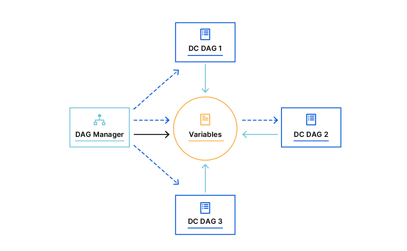
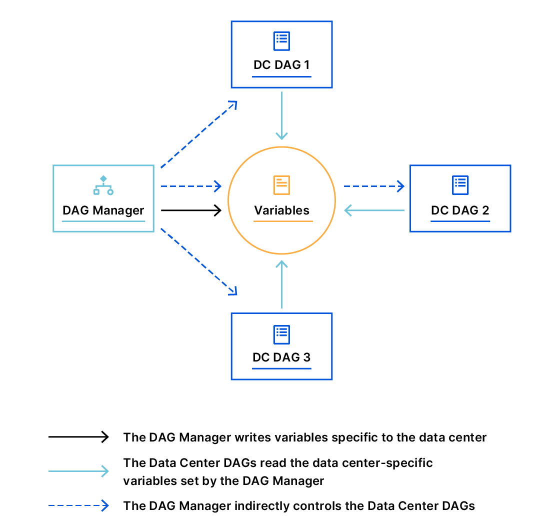
In order for PraaS to be able to accept human inputs, we’ve written a separate DAG we call our DAG Manager. Whenever we need to submit input back to a running expansion DAG, we simply trigger the DAG Manager and pass in our input as a JSON configuration, which will then be processed accordingly and submit the input back to the expansion DAG.
Managing Dependencies Between Tasks
Replacing SOP steps with DAG tasks was only the first part of our journey towards greater automation. We also had to define the dependencies between these tasks and construct the workflow accordingly.
Here’s an example of what this looks like in code:
With the bit shift operator, chaining multiple dependencies becomes concise.
By default, a downstream task will only run if its upstream has succeeded. For a more complex dependency setup, we set a trigger_rule which defines the rule by which the generated task gets triggered.
All operators have a trigger_rule argument. The Airflow scheduler decides whether to run the task or not depending on what rule was specified in the task. An example rule that we use a lot in PraaS is “one_success” — it fires as soon as at least one parent succeeds, and it does not wait for all parents to be done.
Solving Complex Workflows with Branching and Multi-DAGs
Having complex workflows means that we need a workflow to branch, or only go down a certain path, based on an arbitrary condition, which is typically related to something that happened in an upstream task. Branching is used to perform conditional logic, that is, execute a set of tasks based on a condition. We use BranchPythonOperator to achieve this.
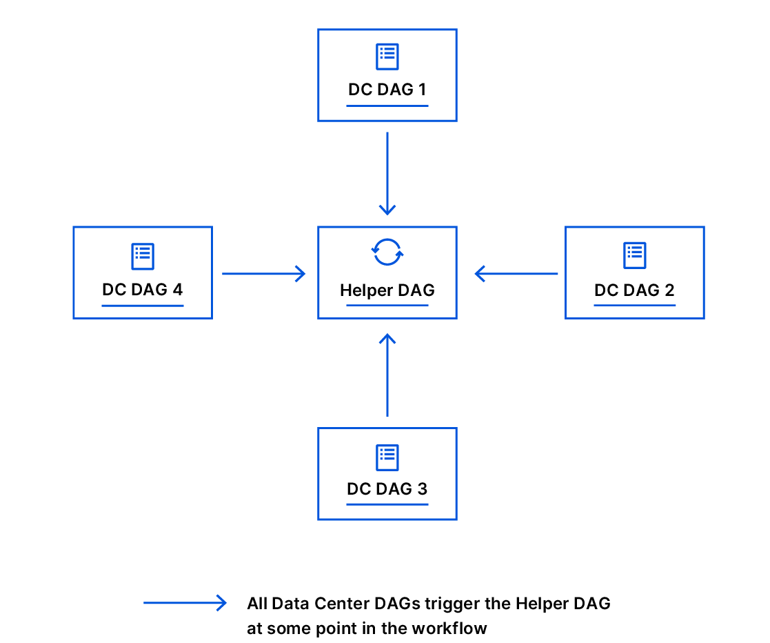
At some point in the workflow, our data center expansion DAGs trigger various external DAGs to accomplish complex tasks. This is why we have written our DAGs to be fully reusable. We did not try to incorporate all the logic into a single DAG; instead, we created other separable DAGs that are fully reusable and can be triggered on-demand manually by hand or programmatically — our DAG Manager and the “helper” DAG is an example of this.
The Helper DAG comprises logic that allows us to mimic a “for loop” by having the DAG respawn itself if needed, technically doing cycles. If you recall, a DAG is acyclic, but we have some tasks in our workflow that require us to do complex loops and are solved by using a helper DAG.
We designed reusable DAGs early on, which allowed us to build complex automation workflows from separable DAGs, each of which handles distinct and well-defined tasks. Each data center DAG could easily reuse other DAGs by triggering them programmatically.
Having separate DAGs that run independently, that are triggered by other DAGs, and that keep inter-dependencies between them, is a pattern we use a lot. It has allowed us to execute very complex workflows.
Creating DAGs that Scale and Executing Tasks at Scale
Data center expansions are done in two phases:
Phase 1 – this is the phase in which servers are powered on. It boots our custom Linux kernel, and begins the provisioning process.
Phase 2 – this is the phase in which newly provisioned servers are enabled in the cluster to receive production traffic.
To reflect these phases in the automation workflow, we also wrote two separate DAGs, one for each phase. However, we have over 200 data centers, so if we were to write a pair of DAGs for each, we would end up writing and maintaining 400 files!
A viable option could be to parameterize our DAGs. At first glance, this approach sounds reasonable. However, it poses one major challenge: tracking the progress of DAG runs will be too difficult and confusing for the human operator using PraaS.
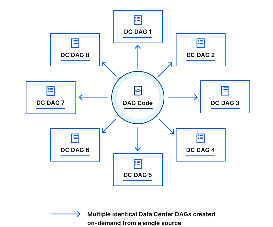
Following the software design principle called DRY (Don’t Repeat Yourself), and inspired by the Factory Method design pattern in programming, we’ve instead written both phase 1 and phase 2 DAGs in a way that allow them to dynamically create multiple different DAGs with exactly the same tasks, and to fully reuse the exact same code. As a result, we only maintain one code base, and as we add new data centers, we are also able to generate a DAG for each new data center instantly, without writing a single line of code.
And Airflow even made it easy to put a simple customized web UI on top of the process, which made it simple to use by more employees who didn’t have to understand all the details.
The death of SOPs?
We would like to think that all of this automation removes the need for our original SOP document. But this is not really the case. Automation can fail, the components in it can fail, and a particular task in the DAG may fail. When this happens, our SOPs will be used again to prevent provisioning and expansion activities from stopping completely.
Introducing automation paved the way for what we call an SOP-as-Code practice. We made sure that every task in the DAG had an equivalent manual step in the SOP that SREs can execute by hand, should the need arise, and that every change in the SOP has a corresponding pull request (PR) in the code.
What’s next for PraaS
Onboarding of the other provisioning activities into PraaS, such as decommissioning, is already ongoing.
For expansions, our ultimate goal is a fully autonomous system that monitors whether new servers have been racked in our edge data centers — and automatically triggers expansions — with no human intervention.
Our fleet of over 200 locations comprises various generations of servers and routers. And with the ever changing landscape of services and computing demands, it’s imperative that we manage power in our data centers right. This blog is a brief Electrical Engineering 101 session going over specifically how power distribution units (PDU) work, along with some good practices on how we use them. It appears to me that we could all use a bit more knowledge on this topic, and more love and appreciation of something that’s critical but usually taken for granted, like hot showers and opposable thumbs.
A PDU is a device used in data centers to distribute power to multiple rack-mounted machines. It’s an industrial grade power strip typically designed to power an average consumption of about seven US households. Advanced models have monitoring features and can be accessed via SSH or webGUI to turn on and off power outlets. How we choose a PDU depends on what country the data center is and what it provides in terms of voltage, phase, and plug type.
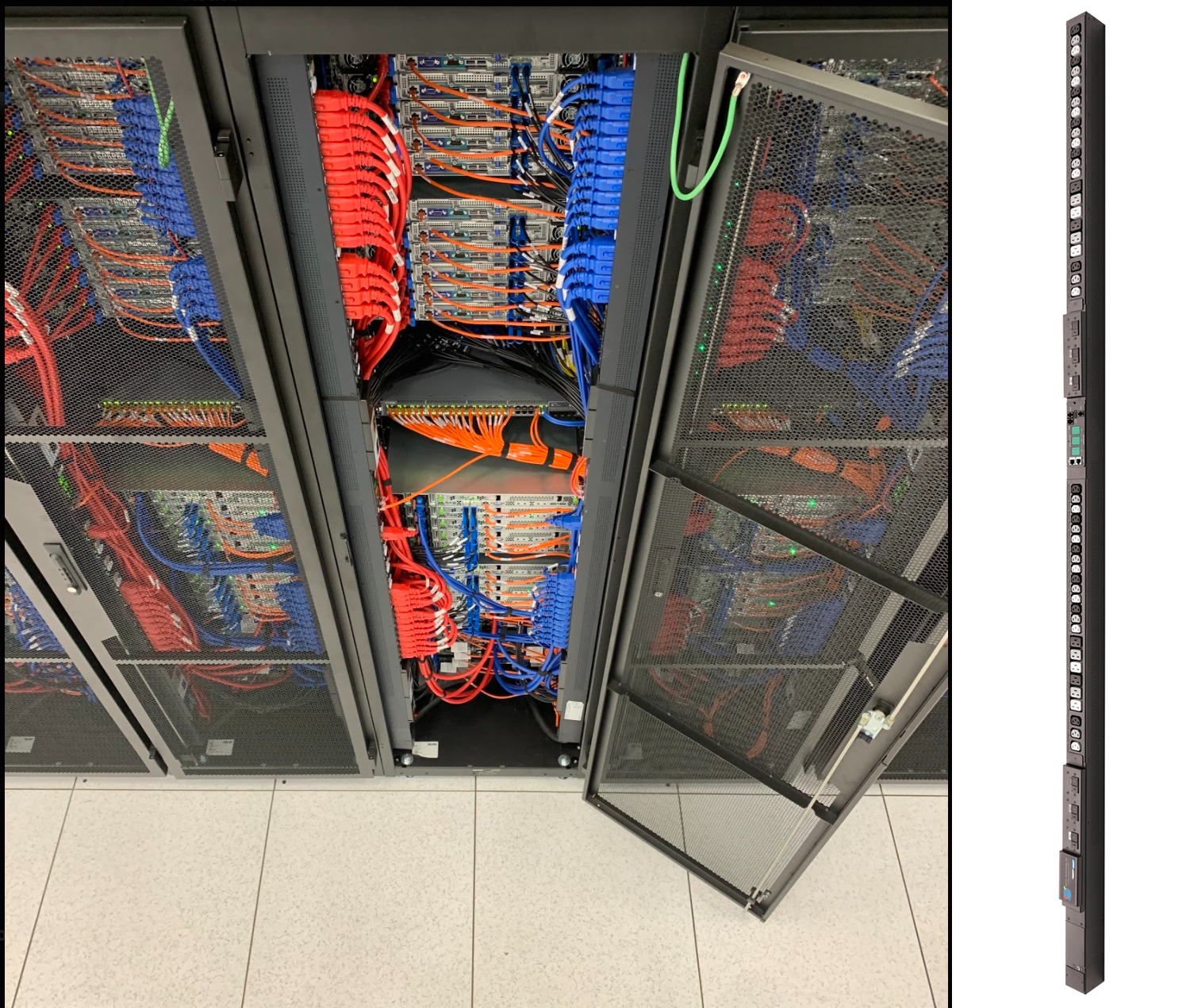
For each of our racks, all of our dual power-supply (PSU) servers are cabled to one of the two vertically mounted PDUs. As shown in the picture above, one PDU feeds a server’s PSU via a red cable, and the other PDU feeds that server’s other PSU via a blue cable. This is to ensure we have power redundancy maximizing our service uptime; in case one of the PDUs or server PSUs fail, the redundant power feed will be available keeping the server alive.
Faraday’s Law and Ohm’s Law
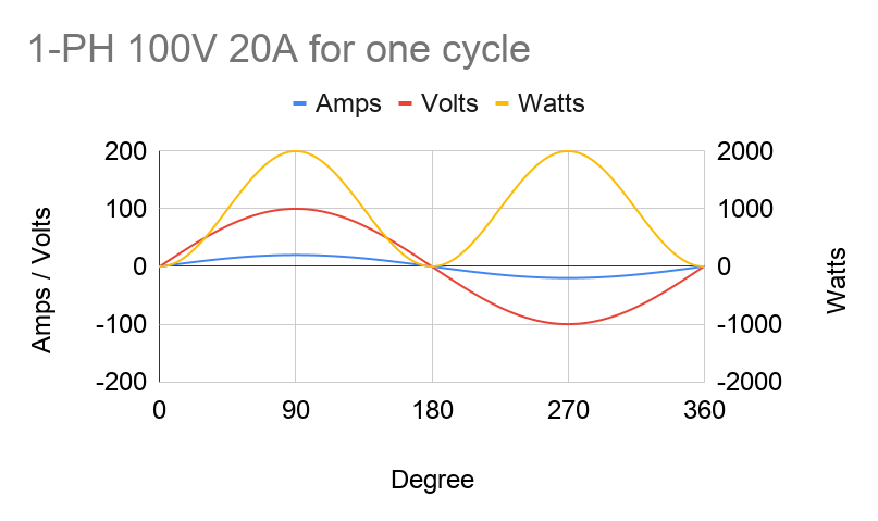
Like most high-voltage applications, PDUs and servers are designed to use AC power. Meaning voltage and current aren’t constant — they’re sine waves with magnitudes that can alternate between positive and negative at a certain frequency. For example, a voltage feed of 100V is not constantly at 100V, but it bounces between 100V and -100V like a sine wave. One complete sine wave cycle is one phase of 360 degrees, and running at 50Hz means there are 50 cycles per second.
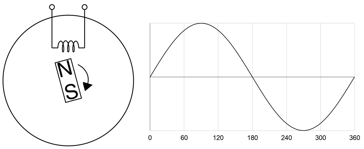
The sine wave can be explained by Faraday’s Law and by looking at how an AC power generator works. Faraday’s Law tells us that a current is induced to flow due to a changing magnetic field. Below illustrates a simple generator with a permanent magnet rotating at constant speed and a coil coming in contact with the magnet’s magnetic field. Magnetic force is strongest at the North and South ends of the magnet. So as it rotates on itself near the coil, current flow fluctuates in the coil. One complete rotation of the magnet represents one phase. As the North end approaches the coil, current increases from zero. Once the North end leaves, current decreases to zero. The South end in turn approaches, now the current “increases” in the opposite direction. And finishing the phase, the South end leaves returning the current back to zero. Current alternates its direction at every half cycle, hence the naming of Alternating Current.
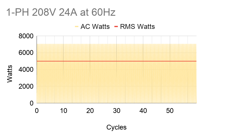
Current and voltage in AC power fluctuate in-phase, or “in tandem”, with each other. So by Ohm’s Law of Power = Voltage x Current, power will always be positive. Notice on the graph below that AC power (Watts) has two peaks per cycle. But for practical purposes, we’d like to use a constant power value. We do that by interpreting AC power into “DC” power using root-mean-square (RMS) averaging, which takes the max value and divides it by √2. For example, in the US, our conditions are 208V 24A at 60Hz. When we look at spec sheets, all of these values can be assumed as RMS’d into their constant DC equivalent values. When we say we’re fully utilizing a PDU’s max capacity of 5kW, it actually means that the power consumption of our machines bounces between 0 and 7.1kW (5kW x √2).
It’s also critical to figure out the sum of power our servers will need in a rack so that it falls under the PDU’s design max power capacity. For our US example, a PDU is typically 5kW (208 volts x 24 amps); therefore, we’re budgeting 5kW and fit as many machines as we can under that. If we need more machines and the total sum power goes above 5kW, we’d need to provision another power source. That would lead to possibly another set of PDUs and racks that we may not fully use depending on demand; e.g. more underutilized costs. All we can do is abide by P = V x I.
However there is a way we can increase the max power capacity economically — 3-phase PDU. Compared to single phase, its max capacity is √3 or 1.7 times higher. A 3-phase PDU of the same US specs above has a capacity of 8.6kW (5kW x √3), allowing us to power more machines under the same source. Using a 3-phase setup might mean it has thicker cables and bigger plug; but despite being more expensive than a 1-phase, its value is higher compared to two 1-phase rack setups for these reasons:
It’s more cost-effective, because there are fewer hardware resources to buy
Say the computing demand adds up to 215kW of hardware, we would need 25 3-phase racks compared to 43 1-phase racks.
Each rack needs two PDUs for power redundancy. Using the example above, we would need 50 3-phase PDUs compared to 86 1-phase PDUs to power 215kW worth of hardware.
That also means a smaller rack footprint and fewer power sources provided and charged by the data center, saving us up to √3 or 1.7 times in opex.
It’s more resilient, because there are more circuit breakers in a 3-phase PDU — one more than in a 1-phase. For example, a 48-outlet PDU that is 1-phase would be split into two circuits of 24 outlets. While a 3-phase one would be split into 3 circuits of 16 outlets. If a breaker tripped, we’d lose 16 outlets using a 3-phase PDU instead of 24.
The PDU shown above is a 3-phase model of 48 outlets. We can see three pairs of circuit breakers for the three branches that are intertwined with each other — white, grey, and black. Industry demands today pressure engineers to maximize compute performance and minimize physical footprint, making the 3-phase PDU a widely-used part of operating a data center.
What is 3-phase?
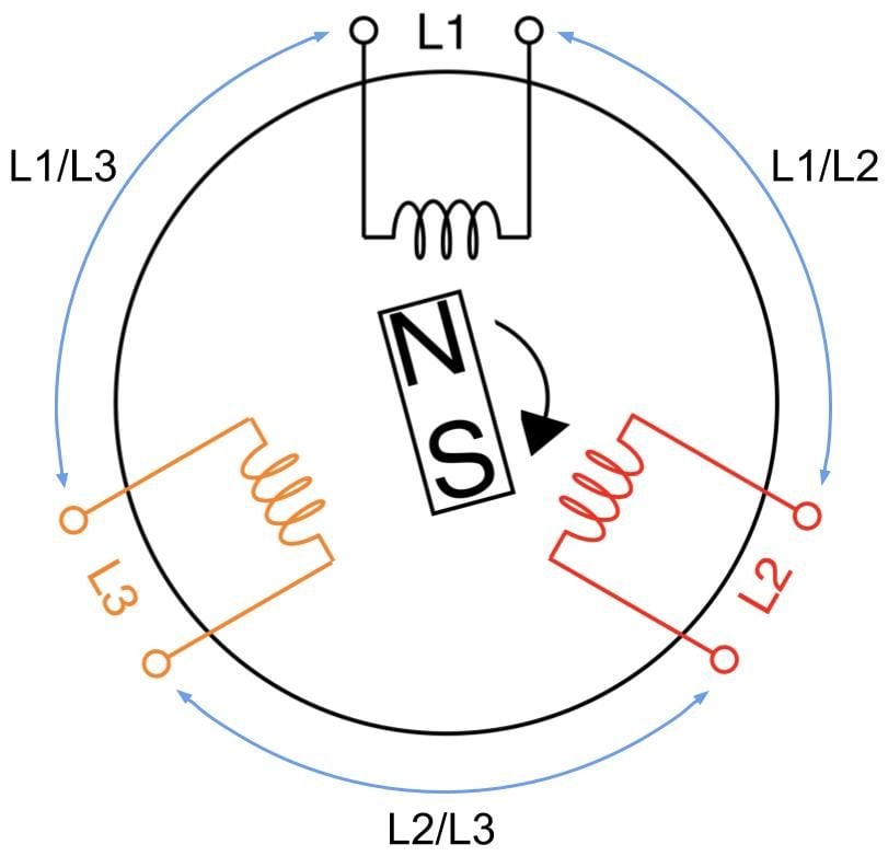
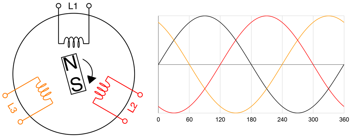
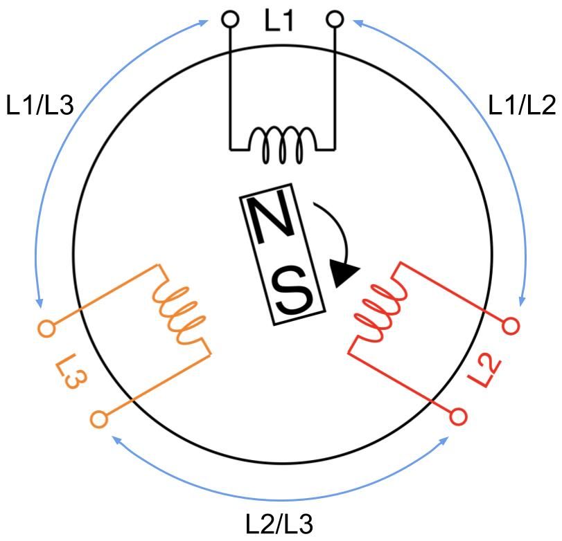
A 3-phase AC generator has three coils instead of one where the coils are 120 degrees apart inside the cylindrical core, as shown in the figure below. Just like the 1-phase generator, current flow is induced by the rotation of the magnet thus creating power from each coil sequentially at every one-third of the magnet’s rotation cycle. In other words, we’re generating three 1-phase power offset by 120 degrees.
A 3-phase feed is set up by joining any of its three coils into line pairs. L1, L2, and L3 coils are live wires with each on their own phase carrying their own phase voltage and phase current. Two phases joining together form one line carrying a common line voltage and line current. L1 and L2 phase voltages create the L1/L2 line voltage. L2 and L3 phase voltages create the L2/L3 line voltage. L1 and L3 phase voltages create the L1/L3 line voltage.
Let’s take a moment to clarify the terminology. Some other sources may refer to line voltage (or current) as line-to-line or phase-to-phase voltage (or current). It can get confusing, because line voltage is the same as phase voltage in 1-phase circuits, as there’s only one phase. Also, the magnitude of the line voltage is equal to the magnitude of the phase voltage in 3-phase Delta circuits, while the magnitude of the line current is equal to the magnitude of the phase current in 3-phase Wye circuits.
Conversely, the line current equals to phase current times √3 in Delta circuits. In Wye circuits, the line voltage equals to phase voltage times √3.
In Delta circuits:
Vline = Vphase
Iline = √3 x Iphase
In Wye circuits:
Vline = √3 x Vphase
Iline = Iphase
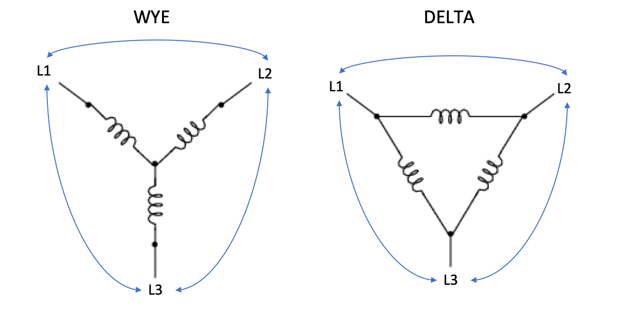
Delta and Wye circuits are the two methods that three wires can join together. This happens both at the power source with three coils and at the PDU end with three branches of outlets. Note that the generator and the PDU don’t need to match each other’s circuit types.
On PDUs, these phases join when we plug servers into the outlets. So we conceptually use the wirings of coils above and replace them with resistors to represent servers. Below is a simplified wiring diagram of a 3-phase Delta PDU showing the three line pairs as three modular branches. Each branch carries two phase currents and its own one common voltage drop.
And this one below is of a 3-phase Wye PDU. Note that Wye circuits have an additional line known as the neutral line where all three phases meet at one point. Here each branch carries one phase and a neutral line, therefore one common current. The neutral line isn’t considered as one of the phases.
Thanks to a neutral line, a Wye PDU can offer a second voltage source that is √3 times lower for smaller devices, like laptops or monitors. Common voltages for Wye PDUs are 230V/400V or 120V/208V, particularly in North America.
Where does the √3 come from?
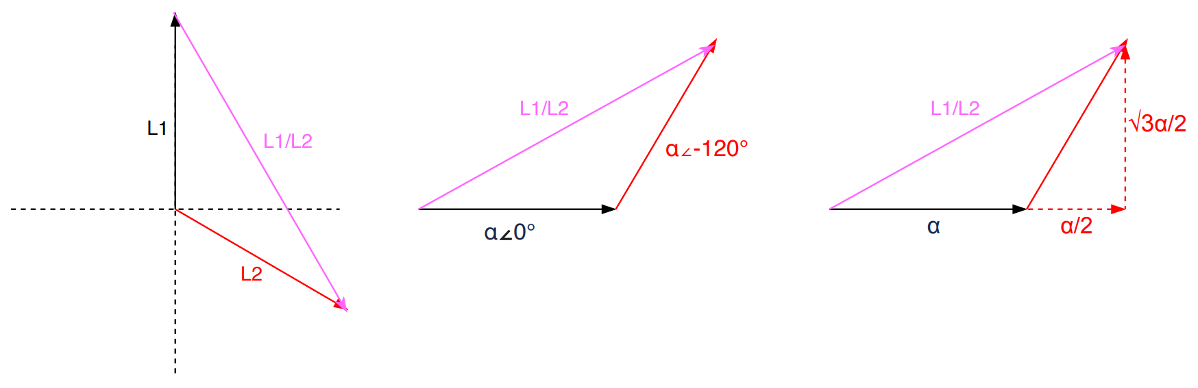
Why are we multiplying by √3? As the name implies, we are adding phasors. Phasors are complex numbers representing sine wave functions. Adding phasors is like adding vectors. Say your GPS tells you to walk 1 mile East (vector a), then walk a 1 mile North (vector b). You walked 2 miles, but you only moved by 1.4 miles NE from the original location (vector a+b). That 1.4 miles of “work” is what we want.
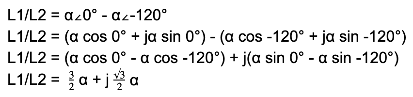
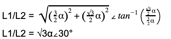
Let’s take in our application L1 and L2 in a Delta circuit. we add phases L1 and L2, we get a L1/L2 line. We assume the 2 coils are identical. Let’s say α represents the voltage magnitude for each phase. The 2 phases are 120 degrees offset as designed in the 3-phase power generator:
Since voltage is a scalar, we’re only interested in the “work”:
|L1/L2| = √3α
Given that α also applies for L3. This means for any of the three line pairs, we multiply the phase voltage by √3 to calculate the line voltage.
Vline = √3 x Vphase
Now with the three line powers being equal, we can add them all to get the overall effective power. The derivation below works for both Delta and Wye circuits.
Poverall = 3 x Pline
Poverall = 3 x (Vline x Iline)
Poverall = (3/√3) x (Vphase x Iphase)
Poverall = √3 x Vphase x Iphase
Using the US example, Vphase is 208V and Iphase is 24A. This leads to the overall 3-phase power to be 8646W (√3 x 208V x 24A) or 8.6kW. There lies the biggest advantage for using 3-phase systems. Adding 2 sets of coils and wires (ignoring the neutral wire), we’ve turned a generator that can produce √3 or 1.7 times more power!
Dealing with 3-phase
The derivation in the section above assumes that the magnitude at all three phases is equal, but we know in practice that’s not always the case. In fact, it’s barely ever. We rarely have servers and switches evenly distributed across all three branches on a PDU. Each machine may have different loads and different specs, so power could be wildly different, potentially causing a dramatic phase imbalance. Having a heavily imbalanced setup could potentially hinder the PDU’s available capacity.
A perfectly balanced and fully utilized PDU at 8.6kW means that each of its three branches has 2.88kW of power consumed by machines. Laid out simply, it’s spread 2.88 + 2.88 + 2.88. This is the best case scenario. If we were to take 1kW worth of machines out of one branch, spreading power to 2.88 + 1.88 + 2.88. Imbalance is introduced, the PDU is underutilized, but we’re fine. However, if we were to put back that 1kW into another branch — like 3.88 + 1.88 + 2.88 — the PDU is over capacity, even though the sum is still 8.6kW. In fact, it would be over capacity even if you just added 500W instead of 1kW on the wrong branch, thus reaching 3.18 + 1.88 + 2.88 (8.1kW).
That’s because a 8.6kW PDU is spec’d to have a maximum of 24A for each phase current. Overloading one of the branches can force phase currents to go over 24A. Theoretically, we can reach the PDU’s capacity by loading one branch until its current reaches 24A and leave the other two branches unused. That’ll render it into a 1-phase PDU, losing the benefit of the √3 multiplier. In reality, the branch would have fuses rated less than 24A (usually 20A) to ensure we won’t reach that high and cause overcurrent issues. Therefore the same 8.6kW PDU would have one of its branches tripped at 4.2kW (208V x 20A).
Loading up one branch is the easiest way to overload the PDU. Being heavily imbalanced significantly lowers PDU capacity and increases risk of failure. To help minimize that, we must:
Ensure that total power consumption of all machines is under the PDU’s max power capacity
Try to be as phase-balanced as possible by spreading cabling evenly across the three branches
Ensure that the sum of phase currents from powered machines at each branch is under the fuse rating at the circuit breaker.
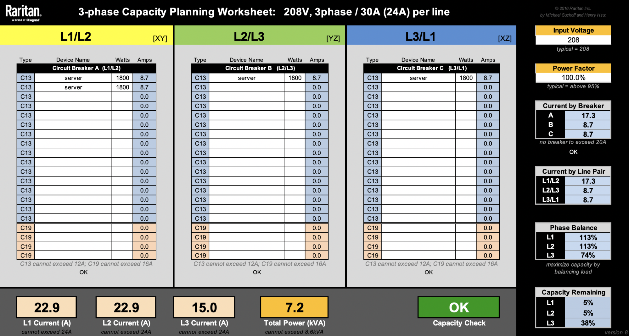
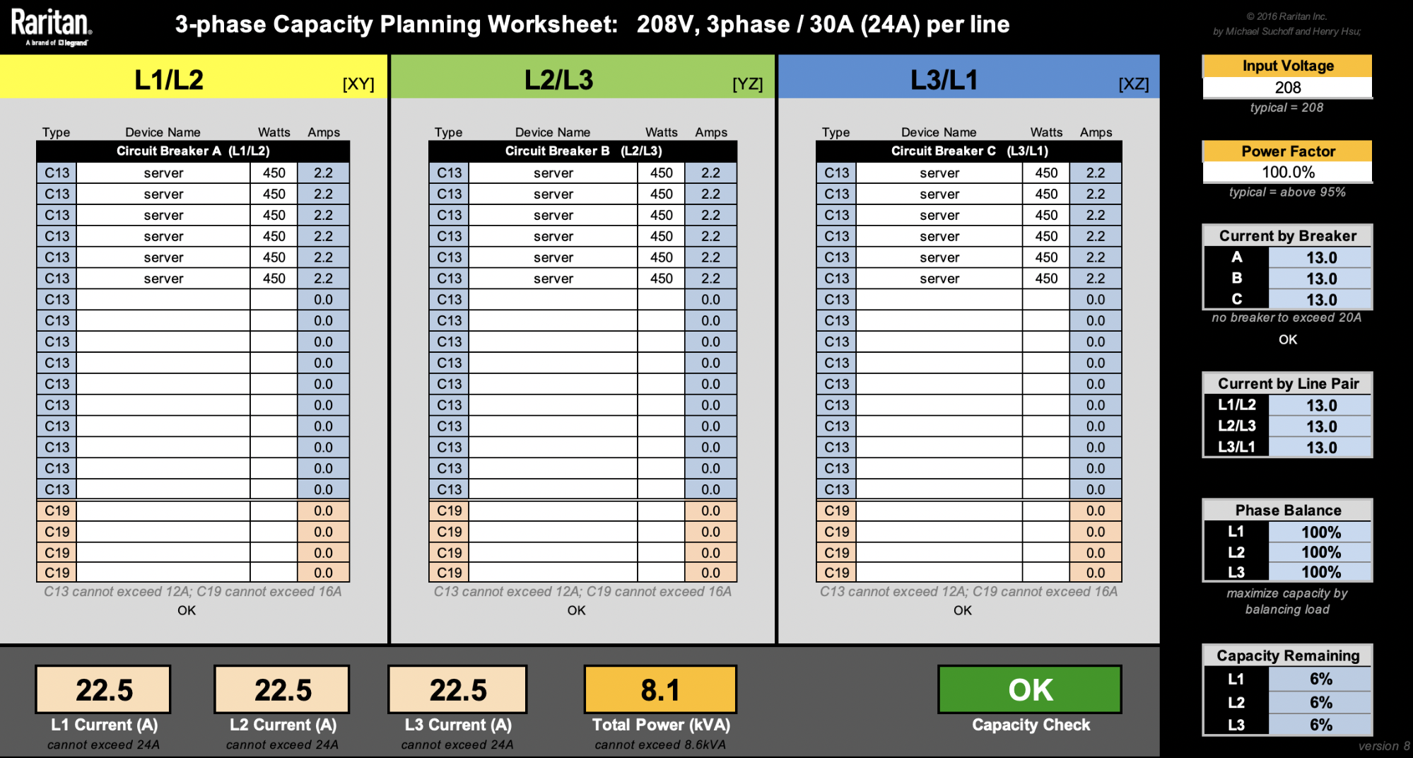
This spreadsheet from Raritan is very useful when designing racks.
For the sake of simplicity, let’s ignore other machines like switches. Our latest 2U4N servers are rated at 1800W. That means we can only fit a maximum of four of these 2U4N chassis (8600W / 1800W = 4.7 chassis). Rounding them up to 5 would reach a total rack level power consumption of 9kW, so that’s a no-no.
Splitting 4 chassis into 3 branches evenly is impossible, and will force us to have one of the branches to have 2 chassis. That would lead to a non-ideal phase balancing:
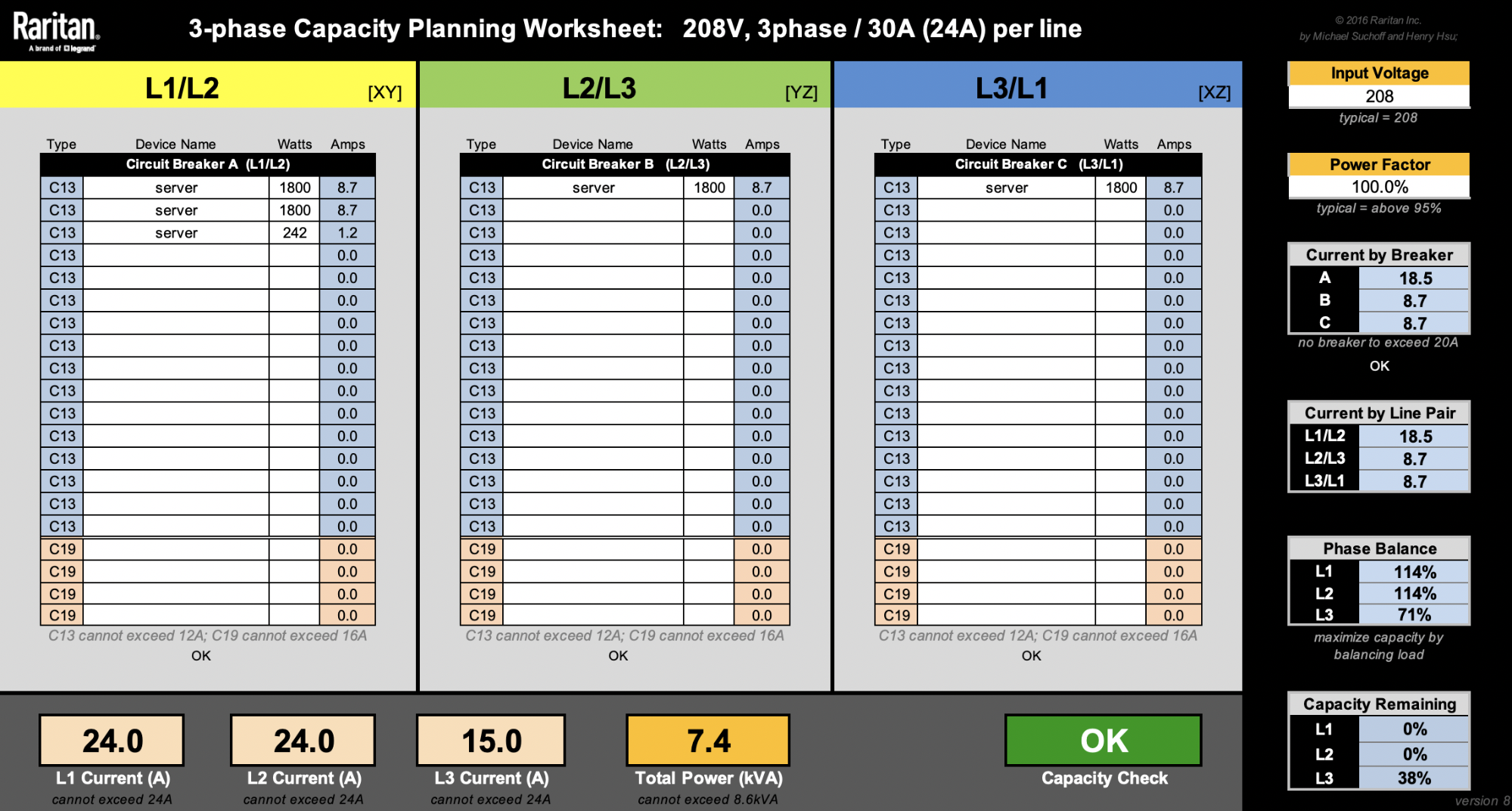
Keeping phase currents under 24A, there’s only 1.1A (24A – 22.9A) to add on L1 or L2 before the PDU gets overloaded. Say we want to add as many machines as we can under the PDU’s power capacity. One solution is we can add up to 242W on the L1/L2 branch until both L1 and L2 currents reach their 24A limit.
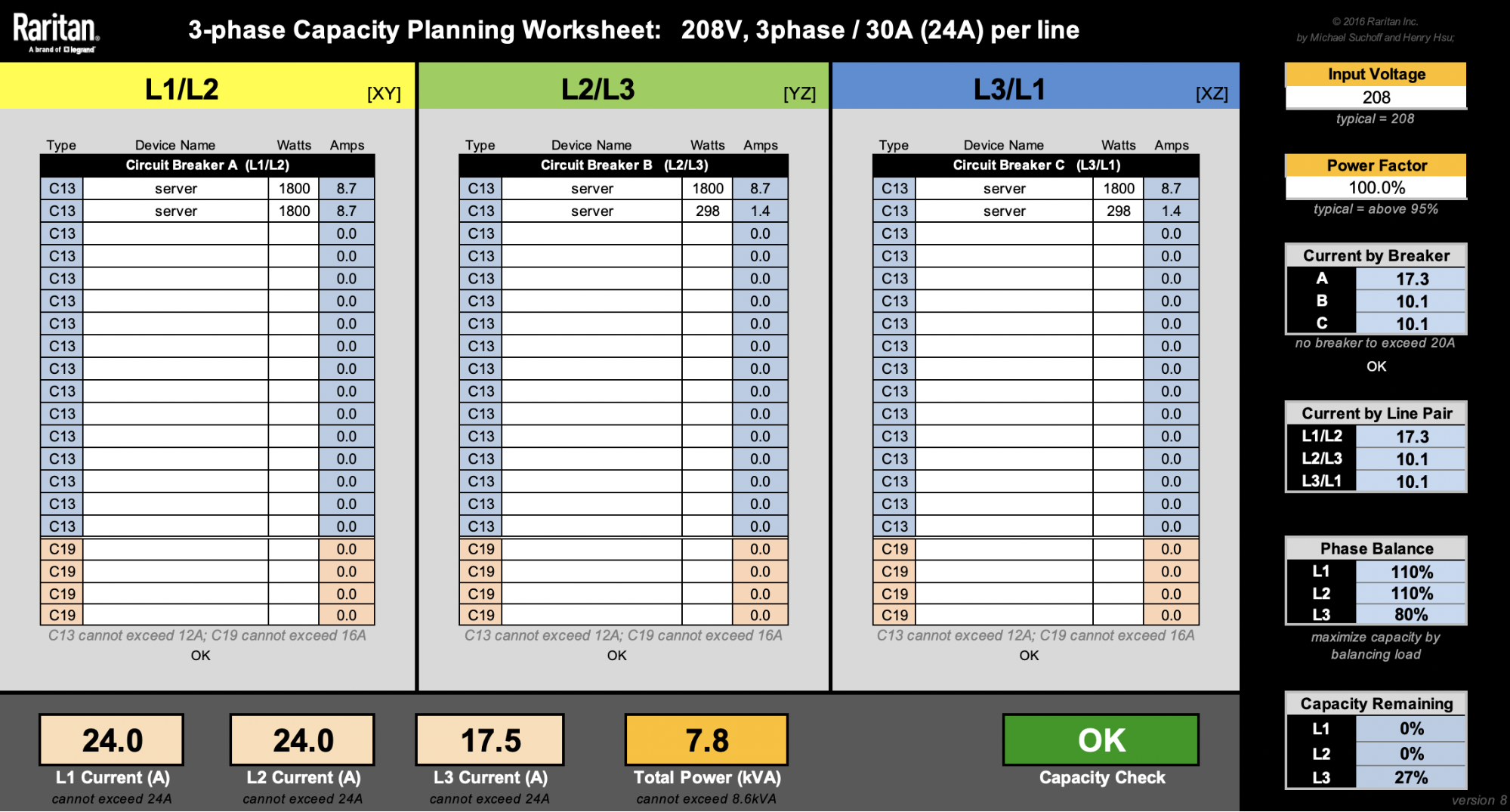
Alternatively, we can add up to 298W on the L2/L3 branch until L2 current reaches 24A. Note we can also add another 298W on the L3/L1 branch until L1 current reaches 24A.
In the examples above, we can see that various solutions are possible. Adding two 298W machines each at L2/L3 and L3/L1 is the most phase balanced solution, given the parameters. Nonetheless, PDU capacity isn’t optimized at 7.8kW.
Dealing with a 1800W server is not ideal, because whichever branch we choose to power one would significantly swing the phase balance unfavorably. Thankfully, our Gen X servers take up less space and are more power efficient. Smaller footprint allows us to have more flexibility and fine-grained control over our racks in many of our diverse data centers. Assuming each 1U server is 450W, as if we physically split the 1800W 2U4N into fours each with their own power supplies, we’re now able to fit 18 nodes. That’s 2 more nodes than the four 2U4N setup:
Adding two more servers here means we’ve increased our value by 12.5%. While there are more factors not considered here to calculate the Total Cost of Ownership, this is still a great way to show we can be smarter with asset costs.
Cloudflare provides the back-end services so that our customers can enjoy the performance, reliability, security, and global scale of our edge network. Meanwhile, we manage all of our hardware in over 100 countries with various power standards and compliances, and ensure that our physical infrastructure is as reliable as it can be.
As the scale of Cloudflare’s edge network has grown, we sometimes reach the limits of parts of our architecture. About two years ago we realized that our existing solution for spreading load within our data centers could no longer meet our needs. We embarked on a project to deploy a Layer 4 Load Balancer, internally called Unimog, to improve the reliability and operational efficiency of our edge network. Unimog has now been deployed in production for over a year.
This post explains the problems Unimog solves and how it works. Unimog builds on techniques used in other Layer 4 Load Balancers, but there are many details of its implementation that are tailored to the needs of our edge network.
The role of Unimog in our edge network
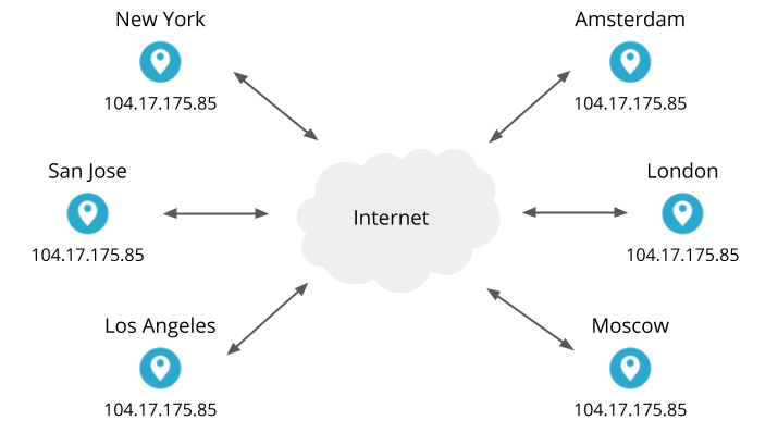
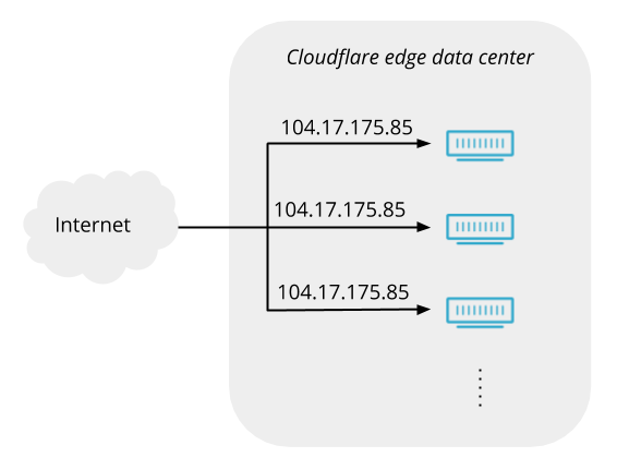
Cloudflare operates an anycast network, meaning that our data centers in 200+ cities around the world serve the same IP addresses. For example, our own cloudflare.com website uses Cloudflare services, and one of its IP addresses is 104.17.175.85. All of our data centers will accept connections to that address and respond to HTTP requests. By the magic of Internet routing, when you visit cloudflare.com and your browser connects to 104.17.175.85, your connection will usually go to the closest (and therefore fastest) data center.
Inside those data centers are many servers. The number of servers in each varies greatly (the biggest data centers have a hundred times more servers than the smallest ones). The servers run the application services that implement our products (our caching, DNS, WAF, DDoS mitigation, Spectrum, WARP, etc). Within a single data center, any of the servers can handle a connection for any of our services on any of our anycast IP addresses. This uniformity keeps things simple and avoids bottlenecks.
But if any server within a data center can handle any connection, when a connection arrives from a browser or some other client, what controls which server it goes to? That’s the job of Unimog.
There are two main reasons why we need this control. The first is that we regularly move servers in and out of operation, and servers should only receive connections when they are in operation. For example, we sometimes remove a server from operation in order to perform maintenance on it. And sometimes servers are automatically removed from operation because health checks indicate that they are not functioning correctly.
The second reason concerns the management of the load on the servers (by load we mean the amount of computing work each one needs to do). If the load on a server exceeds the capacity of its hardware resources, then the quality of service to users will suffer. The performance experienced by users degrades as a server approaches saturation, and if a server becomes sufficiently overloaded, users may see errors. We also want to prevent servers being underloaded, which would reduce the value we get from our investment in hardware. So Unimog ensures that the load is spread across the servers in a data center. This general idea is called load balancing (balancing because the work has to be done somewhere, and so for the load on one server to go down, the load on some other server must go up).
Note that in this post, we’ll discuss how Cloudflare balances the load on its own servers in edge data centers. But load balancing is a requirement that occurs in many places in distributed computing systems. Cloudflare also has a Layer 7 Load Balancing product to allow our customers to balance load across their servers. And Cloudflare uses load balancing in other places internally.
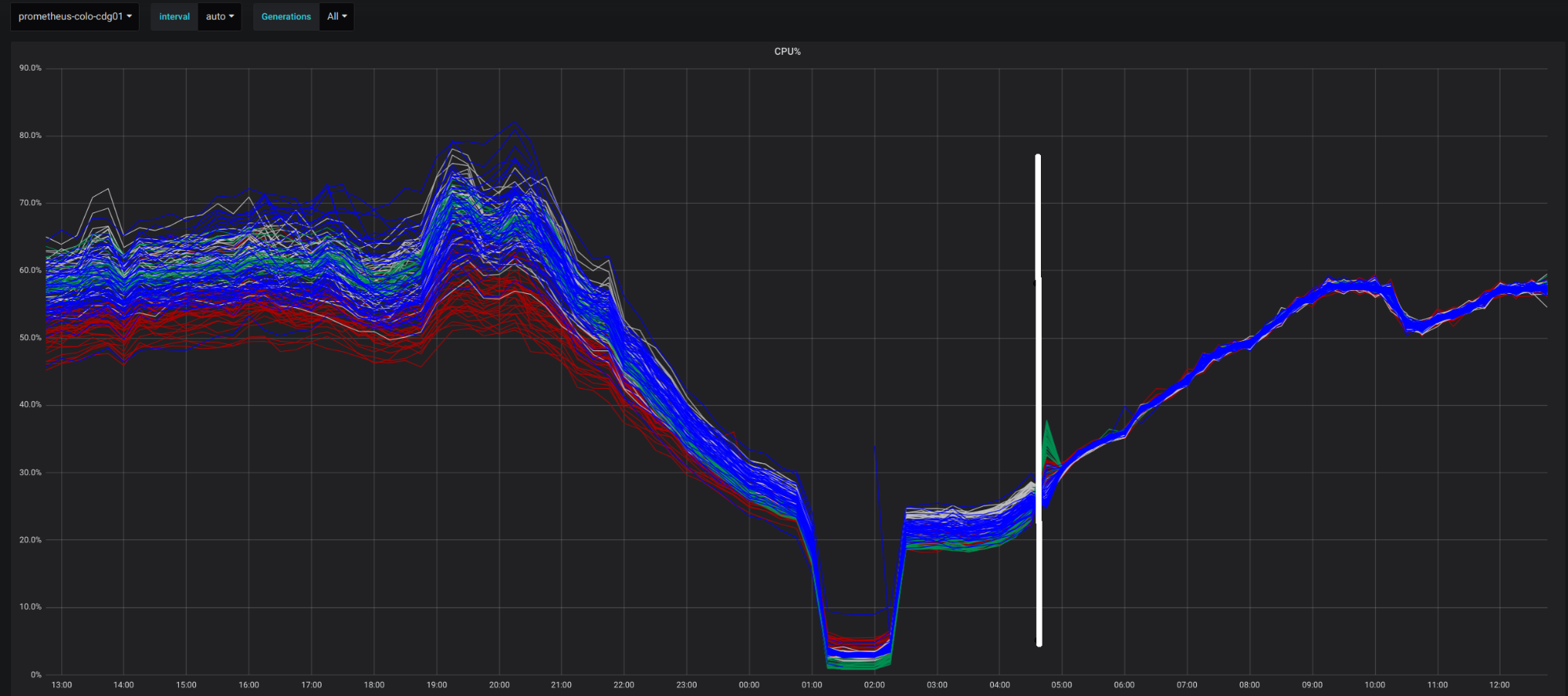
Deploying Unimog led to a big improvement in our ability to balance the load on our servers in our edge data centers. Here’s a chart for one data center, showing the difference due to Unimog. Each line shows the processor utilization of an individual server (the colour of the lines indicates server model). The load on the servers varies during the day with the activity of users close to this data center.The white line marks the point when we enabled Unimog. You can see that after that point, the load on the servers became much more uniform. We saw similar results when we deployed Unimog to our other data centers.
How Unimog compares to other load balancers
There are a variety of techniques for load balancing. Unimog belongs to a category called Layer 4 Load Balancers (L4LBs). L4LBs direct packets on the network by inspecting information up to layer 4 of the OSI network model, which distinguishes them from the more common Layer 7 Load Balancers.
The advantage of L4LBs is their efficiency. They direct packets without processing the payload of those packets, so they avoid the overheads associated with higher level protocols. For any load balancer, it’s important that the resources consumed by the load balancer are low compared to the resources devoted to useful work. At Cloudflare, we already pay close attention to the efficient implementation of our services, and that sets a high bar for the load balancer that we put in front of those services.
The downside of L4LBs is that they can only control which connections go to which servers. They cannot modify the data going over the connection, which prevents them from participating in higher-level protocols like TLS, HTTP, etc. (in contrast, Layer 7 Load Balancers act as proxies, so they can modify data on the connection and participate in those higher-level protocols).
L4LBs are not new. They are mostly used at companies which have scaling needs that would be hard to meet with L7LBs alone. Google has published about Maglev, Facebook open-sourced Katran, and Github has open-sourced their GLB.
Unimog is the L4LB that Cloudflare has built to meet the needs of our edge network. It shares features with other L4LBs, and it is particularly strongly influenced by GLB. But there are some requirements that were not well-served by existing L4LBs, leading us to build our own:
Unimog is designed to run on the same general-purpose servers that provide application services, rather than requiring a separate tier of servers dedicated to load balancing.
It performs dynamic load balancing: measurements of server load are used to adjust the number of connections going to each server, in order to accurately balance load.
It supports long-lived connections that remain established for days.
Virtual IP addresses are managed as ranges (Cloudflare serves hundreds of thousands of IPv4 addresses on behalf of our customers, so it is impractical to configure these individually).
Unimog is tightly integrated with our existing DDoS mitigation system, and the implementation relies on the same XDP technology in the Linux kernel.
The rest of this post describes these features and the design and implementation choices that follow from them in more detail.
For Unimog to balance load, it’s not enough to send the same (or approximately the same) number of connections to each server, because the performance of our servers varies. We regularly update our server hardware, and we’re now on our 10th generation. Once we deploy a server, we keep it in service for as long as it is cost effective, and the lifetime of a server can be several years. It’s not unusual for a single data center to contain a mix of server models, due to expansion and upgrades over time. Processor performance has increased significantly across our server generations. So within a single data center, we need to send different numbers of connections to different servers to utilize the same percentage of their capacity.
It’s also not enough to give each server a fixed share of connections based on static estimates of their capacity. Not all connections consume the same amount of CPU. And there are other activities running on our servers and consuming CPU that are not directly driven by connections from clients. So in order to accurately balance load across servers, Unimog does dynamic load balancing: it takes regular measurements of the load on each of our servers, and uses a control loop that increases or decreases the number of connections going to each server so that their loads converge to an appropriate value.
Refresher: TCP connections
The relationship between TCP packets and connections is central to the operation of Unimog, so we’ll briefly describe that relationship.
(Unimog supports UDP as well as TCP, but for clarity most of this post will focus on the TCP support. We explain how UDP support differs towards the end.)
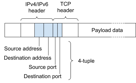
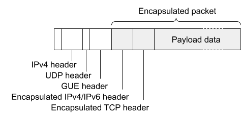
Here is the outline of a TCP packet:
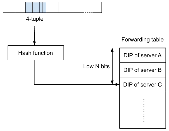
The TCP connection that this packet belongs to is identified by the four labelled header fields, which span the IPv4/IPv6 (i.e. layer 3) and TCP (i.e. layer 4) headers: the source and destination addresses, and the source and destination ports. Collectively, these four fields are known as the 4-tuple. When we say the Unimog sends a connection to a server, we mean that all the packets with the 4-tuple identifying that connection are sent to that server.
A TCP connection is established via a three-way handshake between the client and the server handling that connection. Once a connection has been established, it is crucial that all the incoming packets for that connection go to that same server. If a TCP packet belonging to the connection is sent to a different server, it will signal the fact that it doesn’t know about the connection to the client with a TCP RST (reset) packet. Upon receiving this notification, the client terminates the connection, probably resulting in the user seeing an error. So a misdirected packet is much worse than a dropped packet. As usual, we consider the network to be unreliable, and it’s fine for occasional packets to be dropped. But even a single misdirected packet can lead to a broken connection.
Cloudflare handles a wide variety of connections on behalf of our customers. Many of these connections carry HTTP, and are typically short lived. But some HTTP connections are used for websockets, and can remain established for hours or days. Our Spectrum product supports arbitrary TCP connections. TCP connections can be terminated or stall for many reasons, and ideally all applications that use long-lived connections would be able to reconnect transparently, and applications would be designed to support such reconnections. But not all applications and protocols meet this ideal, so we strive to maintain long-lived connections. Unimog can maintain connections that last for many days.
Forwarding packets
The previous section described that the function of Unimog is to steer connections to servers. We’ll now explain how this is implemented.
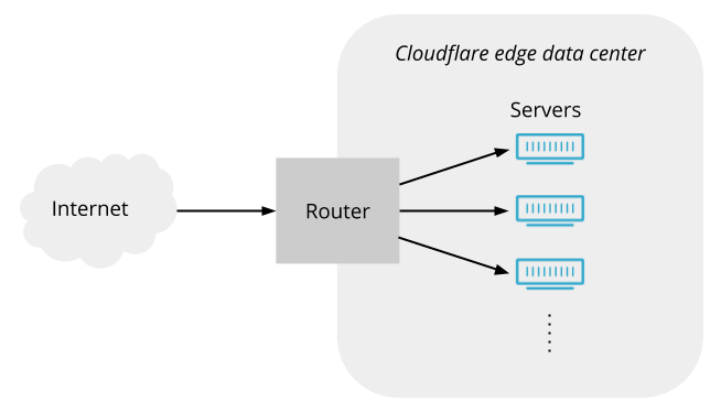
To start with, let’s consider how one of our data centers might look without Unimog or any other load balancer. Here’s a conceptual view:
Packets arrive from the Internet, and pass through the router, which forwards them on to servers (in reality there is usually additional network infrastructure between the router and the servers, but it doesn’t play a significant role here so we’ll ignore it).
But is such a simple arrangement possible? Can the router spread traffic over servers without some kind of load balancer in between? Routers have a feature called ECMP (equal cost multipath) routing. Its original purpose is to allow traffic to be spread across multiple paths between two locations, but it is commonly repurposed to spread traffic across multiple servers within a data center. In fact, Cloudflare relied on ECMP alone to spread load across servers before we deployed Unimog. ECMP uses a hashing scheme to ensure that packets on a given connection use the same path (Unimog also employs a hashing scheme, so we’ll discuss how this can work in further detail below) . But ECMP is vulnerable to changes in the set of active servers, such as when servers go in and out of service. These changes cause rehashing events, which break connections to all the servers in an ECMP group. Also, routers impose limits on the sizes of ECMP groups, which means that a single ECMP group cannot cover all the servers in our larger edge data centers. Finally, ECMP does not allow us to do dynamic load balancing by adjusting the share of connections going to each server. These drawbacks mean that ECMP alone is not an effective approach.
Ideally, to overcome the drawbacks of ECMP, we could program the router with the appropriate logic to direct connections to servers in the way we want. But although programmable network data planes have been a hot research topic in recent years, commodity routers are still essentially fixed-function devices.
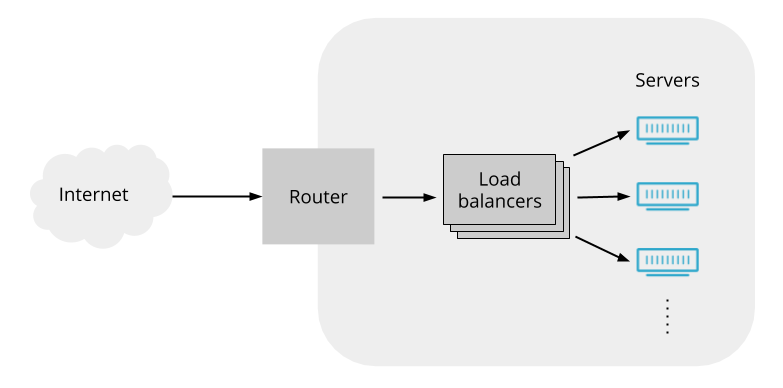
We can work around the limitations of routers by having the router send the packets to some load balancing servers, and then programming those load balancers to forward packets as we want. If the load balancers all act on packets in a consistent way, then it doesn’t matter which load balancer gets which packets from the router (so we can use ECMP to spread packets across the load balancers). That suggests an arrangement like this:
And indeed L4LBs are often deployed like this.
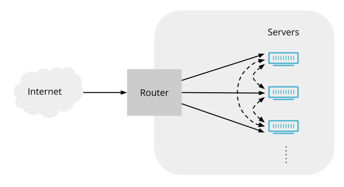
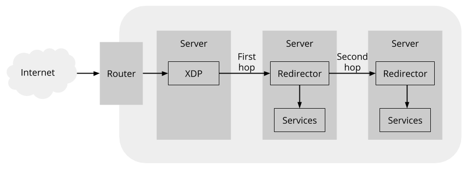
Instead, Unimog makes every server into a load balancer. The router can send any packet to any server, and that initial server will forward the packet to the right server for that connection:
We have two reasons to favour this arrangement:
First, in our edge network, we avoid specialised roles for servers. We run the same software stack on the servers in our edge network, providing all of our product features, whether DDoS attack prevention, website performance features, Cloudflare Workers, WARP, etc. This uniformity is key to the efficient operation of our edge network: we don’t have to manage how many load balancers we have within each of our data centers, because all of our servers act as load balancers.
The second reason relates to stopping attacks. Cloudflare’s edge network is the target of incessant attacks. Some of these attacks are volumetric – large packet floods which attempt to overwhelm the ability of our data centers to process network traffic from the Internet, and so impact our ability to service legitimate traffic. To successfully mitigate such attacks, it’s important to filter out attack packets as early as possible, minimising the resources they consume. This means that our attack mitigation system needs to occur before the forwarding done by Unimog. That mitigation system is called l4drop, and we’ve written about it before. l4drop and Unimog are closely integrated. Because l4drop runs on all of our servers, and because l4drop comes before Unimog, it’s natural for Unimog to run on all of our servers too.
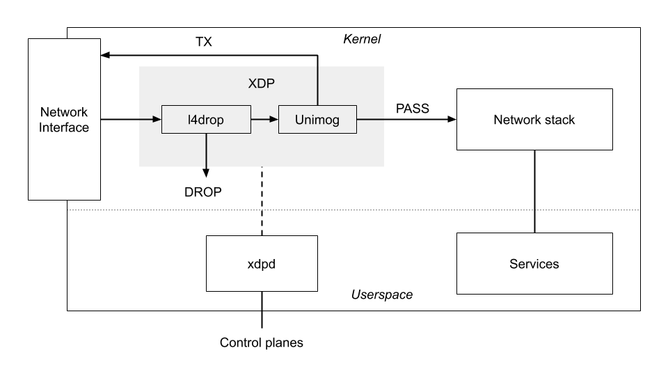
XDP and xdpd
Unimog implements packet forwarding using a Linux kernel facility called XDP. XDP allows a program to be attached to a network interface, and the program gets run for every packet that arrives, before it is processed by the kernel’s main network stack. The XDP program returns an action code to tell the kernel what to do with the packet:
PASS: Pass the packet on to the kernel’s network stack for normal processing.
DROP: Drop the packet. This is the basis for l4drop.
TX: Transmit the packet back out of the network interface. The XDP program can modify the packet data before transmission. This action is the basis for Unimog forwarding.
XDP programs run within the kernel, making this an efficient approach even at high packet rates. XDP programs are expressed as eBPF bytecode, and run within an in-kernel virtual machine. Upon loading an XDP program, the kernel compiles its eBPF code into machine code. The kernel also verifies the program to check that it does not compromise security or stability. eBPF is not only used in the context of XDP: many recent Linux kernel innovations employ eBPF, as it provides a convenient and efficient way to extend the behaviour of the kernel.
XDP is much more convenient than alternative approaches to packet-level processing, particularly in our context where the servers involved also have many other tasks. We have continued to enhance Unimog since its initial deployment. Our deployment model for new versions of our Unimog XDP code is essentially the same as for userspace services, and we are able to deploy new versions on a weekly basis if needed. Also, established techniques for optimizing the performance of the Linux network stack provide good performance for XDP.
There are two main alternatives for efficient packet-level processing:
Kernel-bypass networking (such as DPDK), where a program in userspace manages a network interface (or some part of one) directly without the involvement of the kernel. This approach works best when servers can be dedicated to a network function (due to the need to dedicate processor or network interface hardware resources, and awkward integration with the normal kernel network stack; see our old post about this). But we avoid putting servers in specialised roles. (Github’s open-source GLB uses DPDK, and this is one of the main factors that made GLB unsuitable for us.)
Kernel modules, where code is added to the kernel to perform the necessary network functions. The Linux IPVS (IP Virtual Server) subsystem falls into this category. But developing, testing, and deploying kernel modules is cumbersome compared to XDP.
The following diagram shows an overview of our use of XDP. Both l4drop and Unimog are implemented by an XDP program. l4drop matches attack packets, and uses the DROP action to discard them. Unimog forwards packets, using the TX action to resend them. Packets that are not dropped or forwarded pass through to the normal Linux network stack. To support our elaborate use of XPD, we have developed the xdpd daemon which performs the necessary supervisory and support functions for our XDP programs.
Rather than a single XDP program, we have a chain of XDP programs that must be run for each packet (l4drop, Unimog, and others we have not covered here). One of the responsibilities of xdpd is to prepare these programs, and to make the appropriate system calls to load them and assemble the full chain.
Our XDP programs come from two sources. Some are developed in a conventional way: engineers write C code, our build system compiles it (with clang) to eBPF ELF files, and our release system deploys those files to our servers. Our Unimog XDP code works like this. In contrast, the l4drop XDP code is dynamically generated by xdpd based on information it receives from attack detection systems.
xdpd has many other duties to support our use of XDP:
XDP programs can be supplied with data using data structures called maps. xdpd populates the maps needed by our programs, based on information received from control planes.
Programs (for instance, our Unimog XDP program) may depend upon configuration values which are fixed while the program runs, but do not have universal values known at the time their C code was compiled. It would be possible to supply these values to the program via maps, but that would be inefficient (retrieving a value from a map requires a call to a helper function). So instead, xdpd will fix up the eBPF program to insert these constants before it is loaded.
Cloudflare carefully monitors the behaviour of all our software systems, and this includes our XDP programs: They emit metrics (via another use of maps), which xdpd exposes to our metrics and alerting system (prometheus).
When we deploy a new version of xdpd, it gracefully upgrades in such a way that there is no interruption to the operation of Unimog or l4drop.
Although the XDP programs are written in C, xdpd itself is written in Go. Much of its code is specific to Cloudflare. But in the course of developing xdpd, we have collaborated with Cilium to develop https://github.com/cilium/ebpf, an open source Go library that provides the operations needed by xdpd for manipulating and loading eBPF programs and related objects. We’re also collaborating with the Linux eBPF community to share our experience, and extend the core eBPF technology in ways that make features of xdpd obsolete.
In evaluating the performance of Unimog, our main concern is efficiency: that is, the resources consumed for load balancing relative to the resources used for customer-visible services. Our measurements show that Unimog costs less than 1% of the processor utilization, compared to a scenario where no load balancing is in use. Other L4LBs, intended to be used with servers dedicated to load balancing, may place more emphasis on maximum throughput of packets. Nonetheless, our experience with Unimog and XDP in general indicates that the throughput is more than adequate for our needs, even during large volumetric attacks.
Unimog is not the first L4LB to use XDP. In 2018, Facebook open sourced Katran, their XDP-based L4LB data plane. We considered the possibility of reusing code from Katran. But it would not have been worthwhile: the core C code needed to implement an XDP-based L4LB is relatively modest (about 1000 lines of C, both for Unimog and Katran). Furthermore, we had requirements that were not met by Katran, and we also needed to integrate with existing components and systems at Cloudflare (particularly l4drop). So very little of the code could have been reused as-is.
Encapsulation
As discussed as the start of this post, clients make connections to one of our edge data centers with a destination IP address that can be served by any one of our servers. These addresses that do not correspond to a specific server are known as virtual IPs (VIPs). When our Unimog XDP program forwards a packet destined to a VIP, it must replace that VIP address with the direct IP (DIP) of the appropriate server for the connection, so that when the packet is retransmitted it will reach that server. But it is not sufficient to overwrite the VIP in the packet headers with the DIP, as that would hide the original destination address from the server handling the connection (the original destination address is often needed to correctly handle the connection).
Instead, the packet must be encapsulated: Another set of packet headers is prepended to the packet, so that the original packet becomes the payload in this new packet. The DIP is then used as the destination address in the outer headers, but the addressing information in the headers of the original packet is preserved. The encapsulated packet is then retransmitted. Once it reaches the target server, it must be decapsulated: the outer headers are stripped off to yield the original packet as if it had arrived directly.
Encapsulation is a general concept in computer networking, and is used in a variety of contexts. The headers to be added to the packet by encapsulation are defined by an encapsulation format. Many different encapsulation formats have been defined within the industry, tailored to the requirements in specific contexts. Unimog uses a format called GUE (Generic UDP Encapsulation), in order to allow us to re-use the glb-redirect component from github’s GLB (glb-redirect is discussed below).
GUE is a relatively simple encapsulation format. It encapsulates within a UDP packet, placing a GUE-specific header between the outer IP/UDP headers and the payload packet to allow extension data to be carried (and we’ll see how Unimog takes advantage of this):
When an encapsulated packet arrives at a server, the encapsulation process must be reversed. This step is called decapsulation. The headers that were added during the encapsulation process are removed, leaving the original packet to be processed by the network stack as if it had arrived directly from the client.
An issue that can arise with encapsulation is hitting limits on the maximum packet size, because the encapsulation process makes packets larger. The de-facto maximum packet size on the Internet is 1500 bytes, and not coincidentally this is also the maximum packet size on ethernet networks. For Unimog, encapsulating a 1500-byte packet results in a 1536-byte packet. To allow for these enlarged encapsulated packets, we have enabled jumbo frames on the networks inside our data centers, so that the 1500-byte limit only applies to packets headed out to the Internet.
Forwarding logic
So far, we have described the technology used to implement the Unimog load balancer, but not how our Unimog XDP program selects the DIP address when forwarding a packet. This section describes the basic scheme. But as we’ll see, there is a problem, so then we’ll describe how this scheme is elaborated to solve that problem.
In outline, our Unimog XDP program processes each packet in the following way:
Determine whether the packet is destined for a VIP address. Not all of the packets arriving at a server are for VIP addresses. Other packets are passed through for normal handling by the kernel’s network stack. (xdpd obtains the VIP address ranges from the Unimog control plane.)
Determine the DIP for the server handling the packet’s connection.
Encapsulate the packet, and retransmit it to the DIP.
In step 2, note that all the load balancers must act consistently – when forwarding packets, they must all agree about which connections go to which servers. The rate of new connections arriving at a data center is large, so it’s not practical for load balancers to agree by communicating information about connections amongst themselves. Instead L4LBs adopt designs which allow the load balancers to reach consistent forwarding decisions independently. To do this, they rely on hashing schemes: Take the 4-tuple identifying the packet’s connection, put it through a hash function to obtain a key (the hash function ensures that these key values are uniformly distributed), then perform some kind of lookup into a data structure to turn the key into the DIP for the target server.
Unimog uses such a scheme, with a data structure that is simple compared to some other L4LBs. We call this data structure the forwarding table, and it consists of an array where each entry contains a DIP specifying the server target server for the relevant packets (we call these entries buckets). The forwarding table is generated by the Unimog control plane and broadcast to the load balancers (more on this below), so that it has the same contents on all load balancers.
To look up a packet’s key in the forwarding table, the low N bits from the key are used as the index for a bucket (the forwarding table is always a power-of-2 in size):
Note that this approach does not provide per-connection control – each bucket typically applies to many connections. All load balancers in a data center use the same forwarding table, so they all forward packets in a consistent manner. This means it doesn’t matter which packets are sent by the router to which servers, and so ECMP re-hashes are a non-issue. And because the forwarding table is immutable and simple in structure, lookups are fast.
Although the above description only discusses a single forwarding table, Unimog supports multiple forwarding tables, each one associated with a trafficset – the traffic destined for a particular service. Ranges of VIP addresses are associated with a trafficset. Each trafficset has its own configuration settings and forwarding tables. This gives us the flexibility to differentiate how Unimog behaves for different services.
Precise load balancing requires the ability to make fine adjustments to the number of connections arriving at each server. So we make the number of buckets in the forwarding table more than 100 times the number of servers. Our data centers can contain hundreds of servers, and so it is normal for a Unimog forwarding table to have tens of thousands of buckets. The DIP for a given server is repeated across many buckets in the forwarding table, and by increasing or decreasing the number of buckets that refer to a server, we can control the share of connections going to that server. Not all buckets will correspond to exactly the same number of connections at a given point in time (the properties of the hash function make this a statistical matter). But experience with Unimog has demonstrated that the relationship between the number of buckets and resulting server load is sufficiently strong to allow for good load balancing.
But as mentioned, there is a problem with this scheme as presented so far. Updating a forwarding table, and changing the DIPs in some buckets, would break connections that hash to those buckets (because packets on those connections would get forwarded to a different server after the update). But one of the requirements for Unimog is to allow us to change which servers get new connections without impacting the existing connections. For example, sometimes we want to drain the connections to a server, maintaining the existing connections to that server but not forwarding new connections to it, in the expectation that many of the existing connections will terminate of their own accord. The next section explains how we fix this scheme to allow such changes.
Maintaining established connections
To make changes to the forwarding table without breaking established connections, Unimog adopts the “daisy chaining” technique described in the paper Stateless Datacenter Load-balancing with Beamer.
To understand how the Beamer technique works, let’s look at what can go wrong when a forwarding table changes: imagine the forwarding table is updated so that a bucket which contained the DIP of server A now refers to server B. A packet that would formerly have been sent to A by the load balancers is now sent to B. If that packet initiates a new connection (it’s a TCP SYN packet), there’s no problem – server B will continue the three-way handshake to complete the new connection. On the other hand, if the packet belongs to a connection established before the change, then the TCP implementation of server B has no matching TCP socket, and so sends a RST back to the client, breaking the connection.
This explanation hints at a solution: the problem occurs when server B receives a forwarded packet that does not match a TCP socket. If we could change its behaviour in this case to forward the packet a second time to the DIP of server A, that would allow the connection to server A to be preserved. For this to work, server B needs to know the DIP for the bucket before the change.
To accomplish this, we extend the forwarding table so that each bucket has two slots, each containing the DIP for a server. The first slot contains the current DIP, which is used by the load balancer to forward packets as discussed (and here we refer to this forwarding as the first hop). The second slot preserves the previous DIP (if any), in order to allow the packet to be forwarded again on a second hop when necessary.
For example, imagine we have a forwarding table that refers to servers A, B, and C, and then it is updated to stop new connections going to server A, but maintaining established connections to server A. This is achieved by replacing server A’s DIP in the first slot of any buckets where it appears, but preserving it in the second slot:
In addition to extending the forwarding table, this approach requires a component on each server to forward packets on the second hop when necessary. This diagram shows where this redirector fits into the path a packet can take:
The redirector follows some simple logic to decide whether to process a packet locally on the first-hop server or to forward it on the second-hop server:
If the packet is a SYN packet, initiating a new connection, then it is always processed by the first-hop server. This ensures that new connections go to the first-hop server.
For other packets, the redirector checks whether the packet belongs to a connection with a corresponding TCP socket on the first-hop server. If so, it is processed by that server.
Otherwise, the packet has no corresponding TCP socket on the first-hop server. So it is forwarded on to the second-hop server to be processed there (in the expectation that it belongs to some connection established on the second-hop server that we wish to maintain).
In that last step, the redirector needs to know the DIP for the second hop. To avoid the need for the redirector to do forwarding table lookups, the second-hop DIP is placed into the encapsulated packet by the Unimog XDP program (which already does a forwarding table lookup, so it has easy access to this value). This second-hop DIP is carried in a GUE extension header, so that it is readily available to the redirector if it needs to forward the packet again.
This second hop, when necessary, does have a cost. But in our data centers, the fraction of forwarded packets that take the second hop is usually less than 1% (despite the significance of long-lived connections in our context). The result is that the practical overhead of the second hops is modest.
When we initially deployed Unimog, we adopted the glb-redirect iptables module from github’s GLB to serve as the redirector component. In fact, some implementation choices in Unimog, such as the use of GUE, were made in order to facilitate this re-use. glb-redirect worked well for us initially, but subsequently we wanted to enhance the redirector logic. glb-redirect is a custom Linux kernel module, and developing and deploying changes to kernel modules is more difficult for us than for eBPF-based components such as our XDP programs. This is not merely due to Cloudflare having invested more engineering effort in software infrastructure for eBPF; it also results from the more explicit boundary between the kernel and eBPF programs (for example, we are able to run the same eBPF programs on a range of kernel versions without recompilation). We wanted to achieve the same ease of development for the redirector as for our XDP programs.
To that end, we decided to write an eBPF replacement for glb-redirect. While the redirector could be implemented within XDP, like our load balancer, practical concerns led us to implement it as a TC classifier program instead (TC is the traffic control subsystem within the Linux network stack). A downside to XDP is that the packet contents prior to processing by the XDP program are not visible using conventional tools such as tcpdump, complicating debugging. TC classifiers do not have this downside, and in the context of the redirector, which passes most packets through, the performance advantages of XDP would not be significant.
The result is cls-redirect, a redirector implemented as a TC classifier program. We have contributed our cls-redirect code as part of the Linux kernel test suite. In addition to implementing the redirector logic, cls-redirect also implements decapsulation, removing the need to separately configure GUE tunnel endpoints for this purpose.
There are some features suggested in the Beamer paper that Unimog does not implement:
Beamer embeds generation numbers in the encapsulated packets to address a potential corner case where a ECMP rehash event occurs at the same time as a forwarding table update is propagating from the control plane to the load balancers. Given the combination of circumstances required for a connection to be impacted by this issue, we believe that in our context the number of affected connections is negligible, and so the added complexity of the generation numbers is not worthwhile.
In the Beamer paper, the concept of daisy-chaining encompasses third hops etc. to preserve connections across a series of changes to a bucket. Unimog only uses two hops (the first and second hops above), so in general it can only preserve connections across a single update to a bucket. But our experience is that even with only two hops, a careful strategy for updating the forwarding tables permits connection lifetimes of days.
To elaborate on this second point: when the control plane is updating the forwarding table, it often has some choice in which buckets to change, depending on the event that led to the update. For example, if a server is being brought into service, then some buckets must be assigned to it (by placing the DIP for the new server in the first slot of the bucket). But there is a choice about which buckets. A strategy of choosing the least-recently modified buckets will tend to minimise the impact to connections.
Furthermore, when updating the forwarding table to adjust the balance of load between servers, Unimog often uses a novel trick: due to the redirector logic, exchanging the first-hop and second-hop DIPs for a bucket only affects which server receives new connections for that bucket, and never impacts any established connections. Unimog is able to achieve load balancing in our edge data centers largely through forwarding table changes of this type.
Control plane
So far, we have discussed the Unimog data plane – the part that processes network packets. But much of the development effort on Unimog has been devoted to the control plane – the part that generates the forwarding tables used by the data plane. In order to correctly maintain the forwarding tables, the control plane consumes information from multiple sources:
Server information: Unimog needs to know the set of servers present in a data center, some key information about each one (such as their DIP addresses), and their operational status. It also needs signals about transitional states, such as when a server is being withdrawn from service, in order to gracefully drain connections (preventing the server from receiving new connections, while maintaining its established connections).
Health: Unimog should only send connections to servers that are able to correctly handle those connections, otherwise those servers should be removed from the forwarding tables. To ensure this, it needs health information at the node level (indicating that a server is available) and at the service level (indicating that a service is functioning normally on a server).
Load: in order to balance load, Unimog needs information about the resource utilization on each server.
IP address information: Cloudflare serves hundreds of thousands of IPv4 addresses, and these are something that we have to treat as a dynamic resource rather than something statically configured.
The control plane is implemented by a process called the conductor. In each of our edge data centers, there is one active conductor, but there are also standby instances that will take over if the active instance goes away.
We use Hashicorp’s Consul in a number of ways in the Unimog control plane (we have an independent Consul server cluster in each data center):
Consul provides a key-value store, with support for blocking queries so that changes to values can be received promptly. We use this to propagate the forwarding tables and VIP address information from the conductor to xdpd on the servers.
Consul provides server- and service-level health checks. We use this as the source of health information for Unimog.
The conductor stores its state in the Consul KV store, and uses Consul’s distributed locks to ensure that only one conductor instance is active.
The conductor obtains server load information from Prometheus, which we already use for metrics throughout our systems. It balances the load across the servers using a control loop, periodically adjusting the forwarding tables to send more connections to underloaded servers and less connections to overloaded servers. The load for a server is defined by a Prometheus metric expression which measures processor utilization (with some intricacies to better handle characteristics of our workloads). The determination of whether a server is underloaded or overloaded is based on comparison with the average value of the load metric, and the adjustments made to the forwarding table are proportional to the deviation from the average. So the result of the feedback loop is that the load metric for all servers converges on the average.
Finally, the conductor queries internal Cloudflare APIs to obtain the necessary information on servers and addresses.
Unimog is a critical system: incorrect, poorly adjusted or stale forwarding tables could cause incoming network traffic to a data center to be dropped, or servers to be overloaded, to the point that a data center would have to be removed from service. To maintain a high quality of service and minimise the overhead of managing our many edge data centers, we have to be able to upgrade all components. So to the greatest extent possible, all components are able to tolerate brief absences of the other components without any impact to service. In some cases this is possible through careful design. In other cases, it requires explicit handling. For example, we have found that Consul can temporarily report inaccurate health information for a server and its services when the Consul agent on that server is restarted (for example, in order to upgrade Consul). So we implemented the necessary logic in the conductor to detect and disregard these transient health changes.
Unimog also forms a complex system with feedback loops: The conductor reacts to its observations of behaviour of the servers, and the servers react to the control information they receive from the conductor. This can lead to behaviours of the overall system that are hard to anticipate or test for. For instance, not long after we deployed Unimog we encountered surprising behaviour when data centers became overloaded. This is of course a scenario that we strive to avoid, and we have automated systems to remove traffic from overloaded data centers if it does. But if a data center became sufficiently overloaded, then health information from its servers would indicate that many servers were degraded to the point that Unimog would stop sending new connections to those servers. Under normal circumstances, this is the correct reaction to a degraded server. But if enough servers become degraded, diverting new connections to other servers would mean those servers became degraded, while the original servers were able to recover. So it was possible for a data center that became temporarily overloaded to get stuck in a state where servers oscillated between healthy and degraded, even after the level of demand on the data center had returned to normal. To correct this issue, the conductor now has logic to distinguish between isolated degraded servers and such data center-wide problems. We have continued to improve Unimog in response to operational experience, ensuring that it behaves in a predictable manner over a wide range of conditions.
UDP Support
So far, we have described Unimog’s support for directing TCP connections. But Unimog also supports UDP traffic. UDP does not have explicit connections between clients and servers, so how it works depends upon how the UDP application exchanges packets between the client and server. There are a few cases of interest:
Request-response UDP applications
Some applications, such as DNS, use a simple request-response pattern: the client sends a request packet to the server, and expects a response packet in return. Here, there is nothing corresponding to a connection (the client only sends a single packet, so there is no requirement to make sure that multiple packets arrive at the same server). But Unimog can still provide value by spreading the requests across our servers.
To cater to this case, Unimog operates as described in previous sections, hashing the 4-tuple from the packet headers (the source and destination IP addresses and ports). But the Beamer daisy-chaining technique that allows connections to be maintained does not apply here, and so the buckets in the forwarding table only have a single slot.
UDP applications with flows
Some UDP applications have long-lived flows of packets between the client and server. Like TCP connections, these flows are identified by the 4-tuple. It is necessary that such flows go to the same server (even when Cloudflare is just passing a flow through to the origin server, it is convenient for detecting and mitigating certain kinds of attack to have that flow pass through a single server within one of Cloudflare’s data centers).
It’s possible to treat these flows by hashing the 4-tuple, skipping the Beamer daisy-chaining technique as for request-response applications. But then adding servers will cause some flows to change servers (this would effectively be a form of consistent hashing). For UDP applications, we can’t say in general what impact this has, as we can for TCP connections. But it’s possible that it causes some disruption, so it would be nice to avoid this.
So Unimog adapts the daisy-chaining technique to apply it to UDP flows. The outline remains similar to that for TCP: the same redirector component on each server decides whether to send a packet on a second hop. But UDP does not have anything corresponding to TCP’s SYN packet that indicates a new connection. So for UDP, the part that depends on SYNs is removed, and the logic applied for each packet becomes:
The redirector checks whether the packet belongs to a connection with a corresponding UDP socket on the first-hop server. If so, it is processed by that server.
Otherwise, the packet has no corresponding TCP socket on the first-hop server. So it is forwarded on to the second-hop server to be processed there (in the expectation that it belongs to some flow established on the second-hop server that we wish to maintain).
Although the change compared to the TCP logic is not large, it has the effect of switching the roles of the first- and second-hop servers: For UDP, new flows go to the second-hop server. The Unimog control plane has to take account of this when it updates a forwarding table. When it introduces a server into a bucket, that server should receive new connections or flows. For a TCP trafficset, this means it becomes the first-hop server. For UDP trafficset, it must become the second-hop server.
This difference between handling of TCP and UDP also leads to higher overheads for UDP. In the case of TCP, as new connections are formed and old connections terminate over time, fewer packets will require the second hop, and so the overhead tends to diminish. But with UDP, new connections always involve the second hop. This is why we differentiate the two cases, taking advantage of SYN packets in the TCP case.
The UDP logic also places a requirement on services. The redirector must be able to match packets to the corresponding sockets on a server according to their 4-tuple. This is not a problem in the TCP case, because all TCP connections are represented by connected sockets in the BSD sockets API (these sockets are obtained from an accept system call, so that they have a local address and a peer address, determining the 4-tuple). But for UDP, unconnected sockets (lacking a declared peer address) can be used to send and receive packets. So some UDP services only use unconnected sockets. For the redirector logic above to work, services must create connected UDP sockets in order to expose their flows to the redirector.
UDP applications with sessions
Some UDP-based protocols have explicit sessions, with a session identifier in each packet. Session identifiers allow sessions to persist even if the 4-tuple changes. This happens in mobility scenarios – for example, if a mobile device passes from a WiFi to a cellular network, causing its IP address to change. An example of a UDP-based protocol with session identifiers is QUIC (which calls them connection IDs).
Our Unimog XDP program allows a flow dissector to be configured for different trafficsets. The flow dissector is the part of the code that is responsible for taking a packet and extracting the value that identifies the flow or connection (this value is then hashed and used for the lookup into the forwarding table). For TCP and UDP, there are default flow dissectors that extract the 4-tuple. But specialised flow dissectors can be added to handle UDP-based protocols.
We have used this functionality in our WARP product. We extended the Wireguard protocol used by WARP in a backwards-compatible way to include a session identifier, and added a flow dissector to Unimog to exploit it. There are more details in our post on the technical challenges of WARP.
Conclusion
Unimog has been deployed to all of Cloudflare’s edge data centers for over a year, and it has become essential to our operations. Throughout that time, we have continued to enhance Unimog (many of the features described here were not present when it was first deployed). So the ease of developing and deploying changes, due to XDP and xdpd, has been a significant benefit. Today we continue to extend it, to support more services, and to help us manage our traffic and the load on our servers in more contexts.
Imagine you’re the maintainer of a high-traffic media website, and your DNS is already hosted on Cloudflare.
Page speed is critical. You need to get content to your audience as quickly as possible on every device. You also need to render ads in a speedy way to maintain a good user experience and make money to support your journalism.
One solution would be to render your site statically and cache it at the edge. This would help ensure you have top-notch delivery speed because you don’t need a server to return a response. However, your site has decades worth of content. If you wanted to make even a small change to the site design, you would need to regenerate every single page during your next deploy. This would take ages.
Another issue is that your site would be static — and future updates to content or new articles would not be available until you deploy again.
That’s not going to work.
Another solution would be to render each page dynamically on your server. This ensures you can return a dynamic response for new or updated articles.
However, you’re going to need to pay for some beefy servers to be able to handle spikes in traffic and respond to requests in a timely manner. You’ll also probably need to implement a system of internal caches to optimize the performance of your app, which could lead to a more complicated development experience. That also means you’ll be at risk of a thundering herd problem if, for any reason, your cache becomes invalidated.
Neither of these solutions are great, and you’re forced to make a tradeoff between one of these two approaches.
Thankfully, you’ve recently come across a project like Next.js which offers a hybrid approach: static-site generation along with incremental regeneration. You’re in love with the patterns and developer experience in Next.js, but you’d also love to take advantage of the Cloudflare Workers platform to host your site.
Cloudflare Workers allow you to run your code on the edge quickly, efficiently and at scale. Instead of paying for a server to host your code, you can host it directly inside the datacenter — reducing the number of network trips required to load your application. In a perfect world, we wouldn’t need to find hosting for a Next.js site, because Cloudflare offers the same JavaScript hosting functionality with the Workers platform. With their dynamic runtime and edge caching capabilities, we wouldn’t need to worry about making a tradeoff between static and dynamic for our site.
Unfortunately, frameworks like Next.js and Cloudflare Workers don’t mesh together particularly well due to technical constraints. Until now:
I’m excited to announce Flareact, a new open-source React framework built for Cloudflare Workers.
With Flareact, you don’t need to make the tradeoff between a static site and a dynamic application.
Flareact allows you to render your React apps at the edge rather than on the server. It is modeled after Next.js, which means it supports file-based page routing, dynamic page paths and edge-side data fetching APIs.
Not only are Flareact pages rendered at the edge — they’re also cached at the edge using the Cache API. This allows you to provide a dynamic content source for your app without worrying about traffic spikes or response times.
With no servers or origins to deal with, your site is instantly available to your audience. Cloudflare Workers gives you a 0ms cold start and responses from the edge within milliseconds.
You can check out the docs and get started now by clicking the button below:
To get started manually, install the latest wrangler, and use the handy wrangler generate command below to create your first project:
npm i @cloudflare/wrangler -g
wrangler generate my-project https://github.com/flareact/flareact-template
What’s the big deal?
Hosting React apps on Cloudflare Workers Sites is not a new concept. In fact, you’ve always been able to deploy a create-react-app project to Workers Sites in addition to static versions of other frameworks like Gatsby and Next.js.
However, Flareact renders your React application at the edge. This allows you to provide an initial server response with HTML markup — which can be helpful for search engine crawlers. You can also cache the response at the edge and optionally invalidate that cache on a timed basis — meaning your static markup will be regenerated if you need it to be fresh.
This isn’t a new pattern: Next.js has done the hard work in defining the shape of this API with SSG support and Incremental Static Regeneration. While there are nuanced differences in the implementation between Flareact and Next.js, they serve a similar purpose: to get your application to your end-user in the quickest and most-scalable way possible.
As a longtime fan and user of Next.js, I wanted to experiment with running the framework on Cloudflare Workers. However, Next.js and its APIs are framed around the Node.js HTTP Server API, while Cloudflare Workers use V8 isolates and are modeled after the FetchEvent type.
Since we don’t have typical access to a filesystem inside V8 isolates, it’s tough to mimic the environment required to run a dynamic Next.js server at the edge. Though projects like Fab have come up with workarounds, I decided to approach the project with a clean slate and use existing patterns established in Next.js in a brand-new framework.
As a developer, I absolutely love the simplicity of exporting an asynchronous function from my page to have it supply props to the component. Flareact implements this pattern by allowing you to export a getEdgeProps function. This is similar to getStaticProps in Next.js, and it matches the expected return shape of that function in Next.js — including a revalidate parameter. Learn more about data fetching in Flareact.
I hope porting over an existing Next.js project to Flareact is a breeze!
How it works
When a FetchEvent request comes in, Flareact inspects the URL pathname to decide how to handle it:
If the request is for a page or for page props, it checks the cache for that request and returns it if there’s a hit. If there is a cache miss, it generates the page request or props function, stores the result in the cache, and returns the response.
If the request is for an API route, it sends the entire FetchEvent along to the user-defined API function, allowing the user to respond as they see fit.
If you want your cached page to be revalidated after a certain amount of time, you can return an additional revalidate property from getEdgeProps(). This instructs Flareact to cache the endpoint for that number of seconds before generating a new response.
Finally, if the request is for a static asset, it returns it directly from the Workers KV.
The Worker
The core responsibilities of the Worker — or in a traditional SSR framework, the server —are to:
Render the initial React page component into static HTML markup.
Provide the initial page props as a JSON object, embedded into the static markup in a script tag.
Load the client-side JavaScript bundles and stylesheets necessary to render the interactive page.
One challenge with building Flareact is that the Webpack targets the webworker output rather than the node output. This makes it difficult to inform the worker which pages exist in the filesystem, since there is no access to the filesystem.
To get around this, Flareact leverages require.context, a Webpack-specific API, to inspect the project and build a manifest of pages on the client and the worker. I’d love to replace this with a smarter bundling strategy on the client-side eventually.
The Client
In addition to handling incoming Worker requests, Flareact compiles a client bundle containing the code necessary for routing, data fetching and more from the browser.
The core responsibilities of the client are to:
Listen for routing events
Fetch the necessary page component and its props from the worker over AJAX
Building a client router from scratch has been a challenge. It listens for changes to the internal route state, updates the URL pathname with pushState, makes an AJAX request to the worker for the page props, and then updates the current component in the render tree with the requested page.
It was fun building a flareact/link component similar to next/link:
import Link from "flareact/link";

export default function Index() {
  return (
    <div>
      <Link href="/about">
        <a>Go to About</a>
      </Link>
    </div>
  );
}
I also set out to build a custom version of next/head for Flareact. As it turns out, this was non-trivial! With lots of interesting stuff going on behind the scenes to support SSR and client-side routing events, I decided to make flareact/head a simple wrapper around react-helmet instead:
import Head from "flareact/head";

export default function Index() {
  return (
    <div>
      <Head>
        <title>My page title</title>
      </Head>
      <h1>Hello, world.</h1>
    </div>
  );
}
Local Development
The local developer experience of Flareact leverages the new wrangler dev command, sending server requests through a local tunnel to the Cloudflare edge and back to your machine.
This is a huge win for productivity, since you don’t need to manually build and deploy your application to see how it will perform in a production environment.
It’s also a really exciting update to the serverless toolchain. Running a robust development environment in a serverless world has always been a challenge, since your code is executing in a non-traditional context. Tunneling local code to the edge and back is such a great addition to Cloudflare’s developer experience.
Use cases
Flareact is a great candidate for a lot of Jamstack-adjacent applications, like blogs or static marketing sites.
It could also be used for more dynamic applications, with robust API functions and authentication mechanisms — all implemented using Cloudflare Workers.
Imagine building a high-traffic e-commerce site with Flareact, where both site reliability and dynamic rendering for things like price changes and stock availability are crucial.
There are also untold possibilities for integrating the Workers KV into your edge props or API functions as a first-class database solution. No need to reach for an externally-hosted database!
While the project is still in its early days, here are a couple real-world examples:
I have to be honest: creating a server-side rendered React framework with little prior knowledge was very difficult. There’s still a ton to learn, and Flareact has a long way to go to reach parity with Next.js in the areas of optimization and production-readiness.
Here’s what I’m hoping to add to Flareact in the near future:
Smarter client bundling and Webpack chunks to reduce individual page weight
A more feature-complete client-side router
The ability to extend and customize the root document of the app
Support for more style frameworks (CSS-in-JS, Sass, CSS modules, etc)
A more stable development environment
Documentation and support for environment variables, secrets and KV namespaces
A guide for deploying from GitHub Actions and other CI tools
To provide the best experiences, we use technologies like cookies to store and/or access device information. Consenting to these technologies will allow us to process data such as browsing behavior or unique IDs on this site. Not consenting or withdrawing consent, may adversely affect certain features and functions.
Functional
Always active
The technical storage or access is strictly necessary for the legitimate purpose of enabling the use of a specific service explicitly requested by the subscriber or user, or for the sole purpose of carrying out the transmission of a communication over an electronic communications network.
Preferences
The technical storage or access is necessary for the legitimate purpose of storing preferences that are not requested by the subscriber or user.
Statistics
The technical storage or access that is used exclusively for statistical purposes.The technical storage or access that is used exclusively for anonymous statistical purposes. Without a subpoena, voluntary compliance on the part of your Internet Service Provider, or additional records from a third party, information stored or retrieved for this purpose alone cannot usually be used to identify you.
Marketing
The technical storage or access is required to create user profiles to send advertising, or to track the user on a website or across several websites for similar marketing purposes.