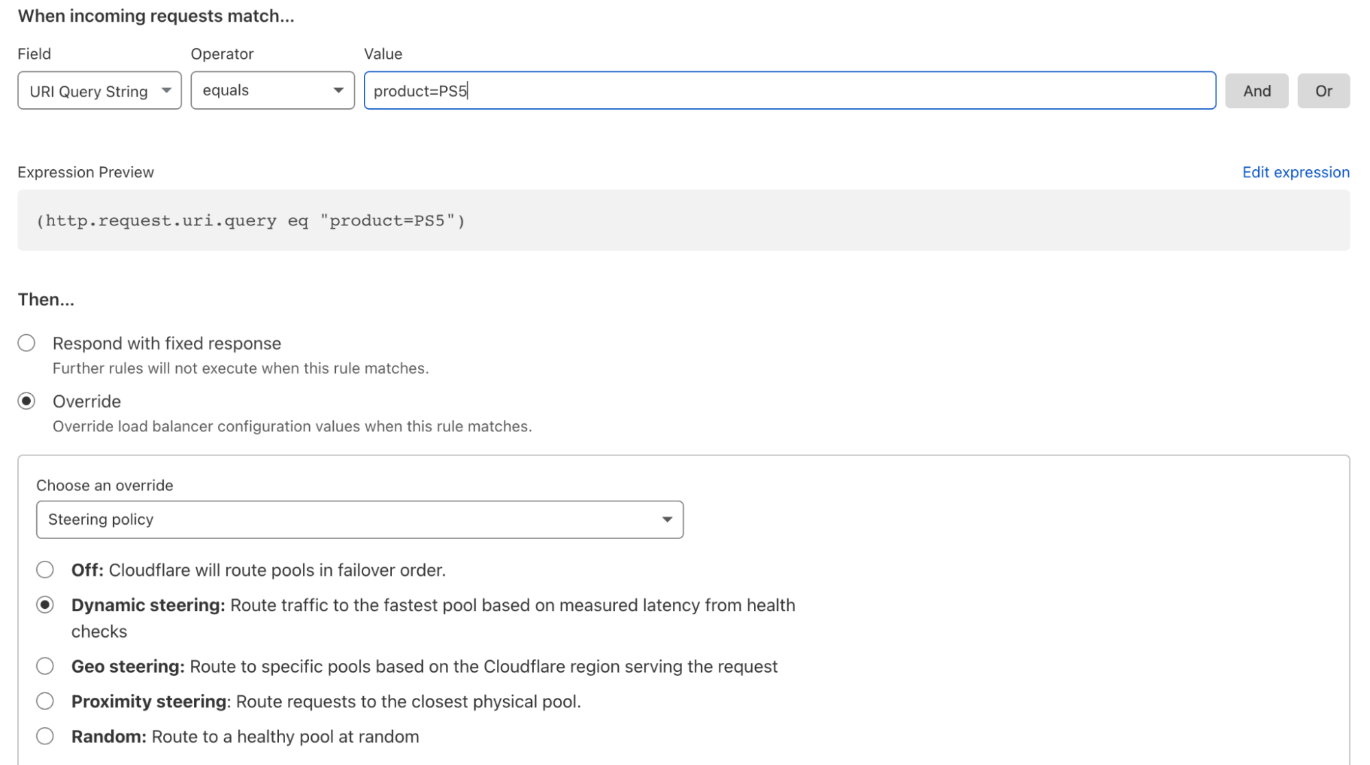
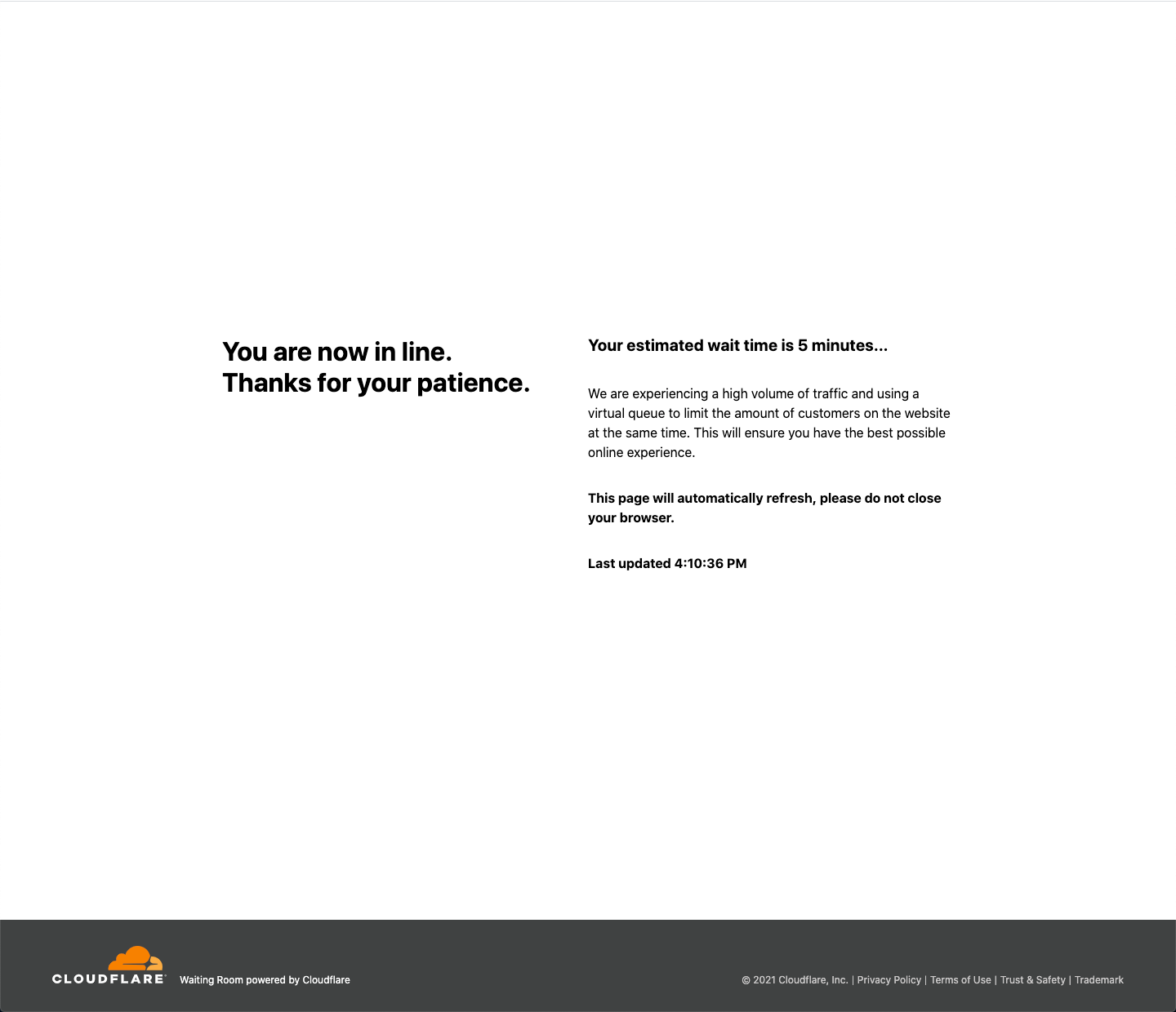
Modern applications are not monoliths. They are complex, distributed systems where availability depends on multiple independent components working in harmony. A web server might be running, but if its connection to the database is down or the authentication service is unresponsive, the application as a whole is unhealthy. Relying on a single health check is like knowing the “check engine” light is not on, but not knowing that one of your tires has a puncture. It’s great your engine is going, but you’re probably not driving far.
As applications grow in complexity, so does the definition of “healthy.” We’ve heard from customers, big and small, that they need to validate multiple services to consider an endpoint ready to receive traffic. For example, they may need to confirm that an underlying API gateway is healthy and that a specific ‘/login’ service is responsive before routing users there. Until now, this required building custom, synthetic services to aggregate these checks, adding operational overhead and another potential point of failure.
Today, we are introducing Monitor Groups for Cloudflare Load Balancing. This feature provides a new way to create sophisticated, multi-service health assessments directly on our platform. With Monitor Groups, you can bundle multiple health monitors into a single logical entity, define which components are critical, and use an aggregated health score to make more intelligent and resilient failover decisions.
This new capability, available via the API for our Enterprise customers, removes the need for custom health aggregation services and provides a far more accurate picture of your application’s true availability. In the near future this feature will be available in the Dashboard for all Load Balancing users, not just Enterprise!
How Monitor Groups Work
Monitor Groups function as a superset of monitors. Once you have created your monitors they can be bundled into a single unit – the Monitor Group! When you attach a Monitor Group to an endpoint pool, the health of each endpoint in that pool is determined by aggregating the results of all enabled monitors within the group. These settings, defined within the ‘members’ array of a monitor group, give you granular control over how the collective health is determined.
// Structure for a single monitor within a group
{
  "description": "Test Monitor Group",
  "members": [
    {
      "monitor_id": "string",
      "enabled": true,
      "monitoring_only": false,
      "must_be_healthy": true
    },
    {
      "monitor_id": "string",
      "enabled": true,
      "monitoring_only": false,
      "must_be_healthy": true
    }
  ]
}
Here’s what each property does:
Critical Monitors (must_be_healthy): You can designate a monitor as critical. If a monitor with this setting fails its health check against an endpoint, that endpoint is immediately marked as unhealthy. This provides a definitive override for essential services, regardless of the status of other monitors in the group.
Observational Probes (monitoring_only): Mark a monitor as “monitoring only” to receive alerts and data without it affecting a pool’s health status or traffic steering. This is perfect for testing new checks or observing non-critical dependencies without impacting production traffic.
Quorum-Based Health: In the absence of a failure from a critical monitor, an endpoint’s health is determined by a quorum of all other active monitors. An endpoint is considered globally unhealthy only if more than 50% of its assigned monitors report it as unhealthy. This system prevents an endpoint from being prematurely marked as unhealthy due to a transient failure from a single, non-critical monitor.
You can add up to five monitors to a group.
A diagram showing three health monitors (HTTP, TCP, and Database) combined into a single Monitor Group. The group is attached to a Cloudflare Load Balancing pool, which assesses the health of three origin servers.
A Globally Distributed Perspective
The power of Monitor Groups is amplified by the scale of Cloudflare’s global network. Health checks aren’t performed from a handful of static locations; they can be configured to execute from data centers in over 300 cities across the globe. While you can configure monitoring from every data center simultaneously (‘All Datacenters’ mode), we recommend a more targeted approach for most applications. Choosing a few diverse regions, like Western North America and Eastern Europe, or using the ‘All Regions’ setting provides a robust, global perspective on your application’s health while reducing the volume of health monitoring traffic sent to your origins. This creates a distributed consensus on application health, preventing a localized network issue from triggering a false positive and causing an unnecessary global failover. Your application’s health is determined not by a single perspective, but by a global one.
This same principle elevates Dynamic Steering when used in conjunction with Monitor Groups. The latency for a Monitor Group isn’t just a single RTT measurement. It’s a holistic performance score, averaged from, potentially, hundreds of points of presence, across all the critical services you’ve defined. This means your load balancer steers traffic based on a true, globally-aware understanding of your application’s performance.
For load balancers using Dynamic Steering and a Monitor Group, the latency used to make steering decisions is now calculated as the average Round Trip Time (RTT) of all active, non-monitoring-only members in the group. This provides a more stable and representative performance metric. Rather than relying on the latency of a single service, Dynamic Steering can now make decisions based on the collective performance of all critical components, ensuring traffic is sent to the endpoint that is truly the most performant overall.
Health Aggregation in Action
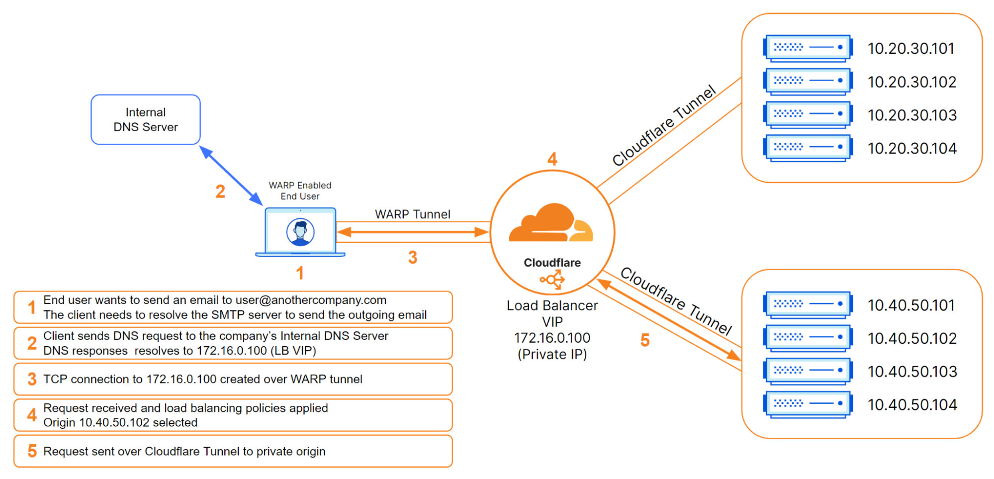
Let’s walk through an example to see how Cloudflare aggregates health signals from a Monitor Group to determine the overall health of a single endpoint. In this scenario, our application has three key components we need to check: a public-facing /health endpoint, another service running on a specific TCP port, and a database dependency. Privacy and security are paramount, so, to monitor the database without exposing it to the public Internet, you would securely connect it to Cloudflare using a Cloudflare Tunnel, allowing our health checks to reach it securely.
Setup
Health Monitors in the Group:
HTTP check for /health (must_be_healthy: true)
TCP check for Port 3000 connectivity (must_be_healthy: false)
DB check for database health (must_be_healthy: false)
Health Check Regions:
Western North America (3 data centers)
Eastern North America (3 data centers)
Quorum Threshold: An endpoint is considered healthy if more than 50% of checking data centers report it as UP.
First, Cloudflare determines the health from the perspective of each individual data center. If the critical monitor fails, that data center’s result is definitively DOWN. Otherwise, the result is based on the majority status of the remaining monitors.
Here are the results from our six data centers:
[image description: A table showing health check results from six data centers across two regions. One of the six data centers report a “DOWN” status because the critical HTTP monitor failed. The other five report “UP” because the critical monitor passed and a majority of the remaining monitors were healthy.]
Finally, the results from all six checking data centers are combined to determine the final, global health status for the endpoint.
Global Result: 5 out of the 6 total data centers (83%) report the endpoint as UP.
Conclusion: Because 83% is greater than the 50% quorum threshold, the endpoint is considered globally healthy and will continue to receive traffic.
This multi-layered quorum system provides incredible resilience, ensuring that failover decisions are based on a comprehensive and geographically distributed consensus.
Getting Started with Monitor Groups
Monitor Groups are now available via the API for all customers with an Enterprise Cloudflare Load Balancing subscription and will be made available to self-serve customers in the near future. To get started with building more sophisticated health checks for your applications today, check out our developer documentation.
POST accounts/{account_id}/load_balancers/monitor_groups
{
  "description": "Monitor group for checkout service",
  "members": [
    {
      "monitor_id": "string",
      "must_be_healthy": true,
	"enabled": true
    },
    {
      "monitor_id": "string",
      "monitoring_only": false,
	"enabled": true
    }
  ]
}
Once created, you can attach the group to a pool by referencing its ID in the monitor_group field of the pool object.
What’s Next
We are continuing to build a seamless platform experience that simplifies traffic management for both internal and external applications. Looking ahead, Monitor Groups will be making its way into the Dashboard for all users soon! We are also working on more flexible role-based access controls and even more advanced load-based load balancing capabilities to give you the granular control you need to manage your most complex applications.
A TURN server helps maintain connections during video calls when local networking conditions prevent participants from connecting directly to other participants. It acts as an intermediary, passing data between users when their networks block direct communication. TURN servers ensure that peer-to-peer calls go smoothly, even in less-than-ideal network conditions.
When building their own TURN infrastructure, developers often have to answer a few critical questions:
“How do we build and maintain a mesh network that achieves near-zero latency to all our users?”
“Where should we spin up our servers?”
“Can we auto-scale reliably to be cost-efficient without hurting performance?”
In April, we launched Cloudflare Calls TURN in open beta to help answer these questions. Starting today, Cloudflare Calls’ TURN service is now generally available to all Cloudflare accounts. Our TURN server works on our anycast network, which helps deliver global coverage and near-zero latency required by real time applications.
TURN solves connectivity and privacy problems for real time apps
When Internet Protocol version 4 (IPv4, RFC 791) was designed back in 1981, it was assumed that the 32-bit address space was big enough for all computers to be able to connect to each other. When IPv4 was created, billions of people didn’t have smartphones in their pockets and the idea of the Internet of Things didn’t exist yet. It didn’t take long for companies, ISPs, and even entire countries to realize they didn’t have enough IPv4 address space to meet their needs.
NATs are unpredictable
Fortunately, you can have multiple devices share the same IP address because the most common protocols run on top of IP are TCP and UDP, both of which support up to 65,535 port numbers. (Think of port numbers on an IP address as extensions behind a single phone number.) To solve this problem of IP scarcity, network engineers developed a way to share a single IP address across multiple devices by exploiting the port numbers. This is called Network Address Translation (NAT) and it is a process through which your router knows which packets to send to your smartphone versus your laptop or other devices, all of which are connecting to the public Internet through the IP address assigned to the router.
In a typical NAT setup, when a device sends a packet to the Internet, the NAT assigns a random, unused port to track it, keeping a forwarding table to map the device to the port. This allows NAT to direct responses back to the correct device, even if the source IP address and port vary across different destinations. The system works as long as the internal device initiates the connection and waits for the response.
However, real-time apps like video or audio calls are more challenging with NAT. Since NATs don’t reveal how they assign ports, devices can’t pre-communicate where to send responses, making it difficult to establish reliable connections. Earlier solutions like STUN (RFC 3489) couldn’t fully solve this, which gave rise to the TURN protocol.
TURN predictably relays traffic between devices while ensuring minimal delay, which is crucial for real-time communication where even a second of lag can disrupt the experience.
ICE to determine if a relay server is needed
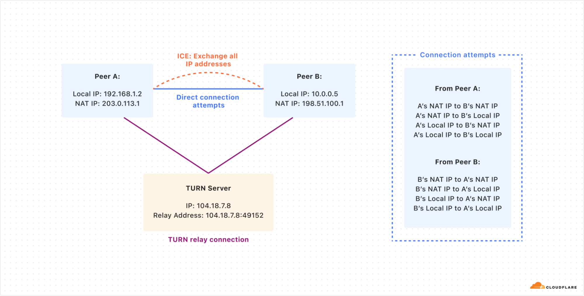
The ICE (Interactive Connectivity Establishment) protocol was designed to find the fastest communication path between devices. It works by testing multiple routes and choosing the one with the least delay. ICE determines whether a TURN server is needed to relay the connection when a direct peer-to-peer path cannot be established or is not performant enough.
How two peers (A and B) try to connect directly by sharing their public and local IP addresses using the ICE protocol. If the direct connection fails, both peers use the TURN server to relay their connection and communicate with each other.
While ICE is designed to find the most efficient connection path between peers, it can inadvertently expose sensitive information, creating privacy concerns. During the ICE process, endpoints exchange a list of all possible network addresses, including local IP addresses, NAT IP addresses, and TURN server addresses. This comprehensive sharing of network details can reveal information about a user’s network topology, potentially exposing their approximate geographic location or details about their local network setup.
The “brute force” nature of ICE, where it attempts connections on all possible paths, can create distinctive network traffic patterns that sophisticated observers might use to infer the use of specific applications or communication protocols.
TURN solves privacy problems
The threat from exposing sensitive information while using real-time applications is especially important for people that use end-to-end encrypted messaging apps for sensitive information — for example, journalists who need to communicate with unknown sources without revealing their location.
With Cloudflare TURN in place, traffic is proxied through Cloudflare, preventing either party in the call from seeing client IP addresses or associated metadata. Cloudflare simply forwards the calls to their intended recipients, but never inspects the contents — the underlying call data is always end-to-end encrypted. This masking of network traffic is an added layer of privacy.
Cloudflare is a trusted third-party when it comes to operating these types of services: we have experience operating privacy-preserving proxies at scale for our Consumer WARP product, Apple’s Private Relay, and Microsoft Edge’s Secure Network, preserving end-user privacy without sacrificing performance.
Cloudflare’s TURN is the fastest because of Anycast
Lots of real time communication services run their own TURN servers on a commercial cloud provider because they don’t want to leave a certain percentage of their customers with non-working communication. This results in additional costs for DevOps, egress bandwidth, etc. And honestly, just deploying and running a TURN server, like CoTURN, in a VPS isn’t an interesting project for most engineers.
Because using a TURN relay adds extra delay for the packets to travel between the peers, the relays should be located as close as possible to the peers. Cloudflare’s TURN service avoids all these headaches by simply running in all of the 330 cities where Cloudflare has data centers. And any time Cloudflare adds another city, the TURN service automatically becomes available there as well.
Anycast is the perfect network topology for TURN
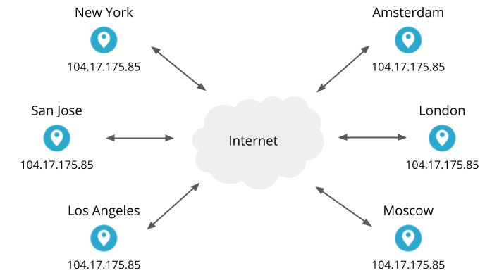
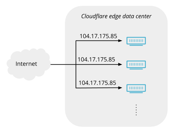
Anycast is a network addressing and routing methodology in which a single IP address is shared by multiple servers in different locations. When a client sends a request to an anycast address, the network automatically routes the request via BGP to the topologically nearest server. This is in contrast to unicast, where each destination has a unique IP address. Anycast allows multiple servers to have the same IP address, and enables clients to automatically connect to a server close to them. This is similar to emergency phone networks (911, 112, etc.) which connect you to the closest emergency communications center in your area.
Anycast allows for lower latency because of the sheer number of locations available around the world. Approximately 95% of the Internet-connected population globally is within approximately 50ms away from a Cloudflare location. For real-time communication applications that use TURN, leads to improved call quality and user experience.
Auto-scaling and inherently global
Running TURN over anycast allows for better scalability and global distribution. By naturally distributing load across multiple servers based on network topology, this setup helps balance traffic and improve performance. When you use Cloudflare’s TURN service, you don’t need to manage a list of servers for different parts of the world. And you don’t need to write custom scaling logic to scale VMs up or down based on your traffic.
Anycast allows TURN to use fewer IP addresses, making it easier to allowlist in restrictive networks. Stateless protocols like DNS over UDP work well with anycast. This includes stateless STUN binding requests used to determine a system’s external IP address behind a NAT.
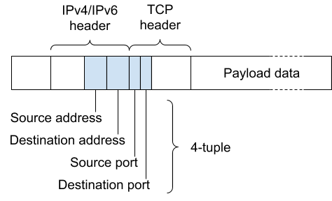
However, stateful protocols over UDP, like QUIC or TURN, are more challenging with anycast. QUIC handles this better due to its stable connection ID, which load balancers can use to consistently route traffic. However, TURN/STUN lacks a similar connection ID. So when a TURN client sends requests to the Cloudflare TURN service, the Unimog load balancer ensures that all its requests get routed to the same server within a data center. The challenges for the communication between a client on the Internet and Cloudflare services listening on an anycast IP address have been described multiple times before.
How does Cloudflare’s TURN server receive packets?
TURN servers act as relay points to help connect clients. This process involves two types of connections: the client-server connection and the third-party connection (relayed address).
The client-server connection uses published IP and port information to communicate with TURN clients using anycast.
For the relayed address, using anycast poses a challenge. The TURN protocol requires that packets reach the specific Cloudflare server handling the client connection. If we used anycast for relay addresses, packets might not arrive at the correct data center or server.
One alternative is to use unicast addresses for relay candidates. However, this approach has drawbacks, including making servers vulnerable to attacks and requiring many IP addresses.
To solve these issues, we’ve developed a middle-ground solution, previously discussed in “Cloudflare servers don’t own IPs anymore – so how do they connect to the Internet?”. We use anycast addresses but add extra handling for packets that reach incorrect servers. If a packet arrives at the wrong Cloudflare location, we forward it over our backbone to the correct datacenter, rather than sending it back over the public Internet.
This approach not only resolves routing issues but also improves TURN connection speed. Packets meant for the relay address enter the Cloudflare network as close to the sender as possible, optimizing the routing process.
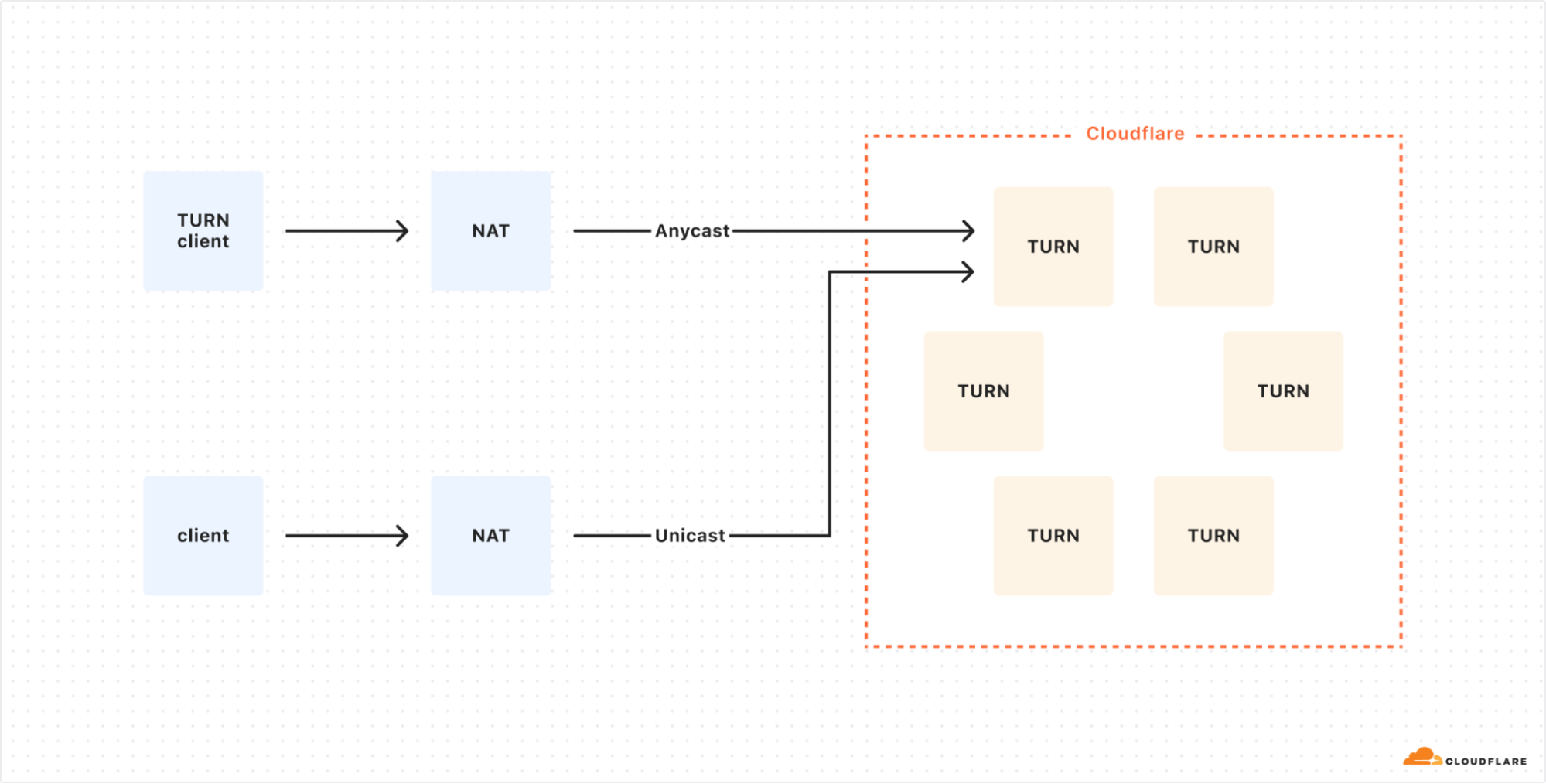
In this non-ideal setup, a TURN client connects to Cloudflare using Anycast, while a direct client uses Unicast, which would expose the TURN server to potential DDoS attacks.
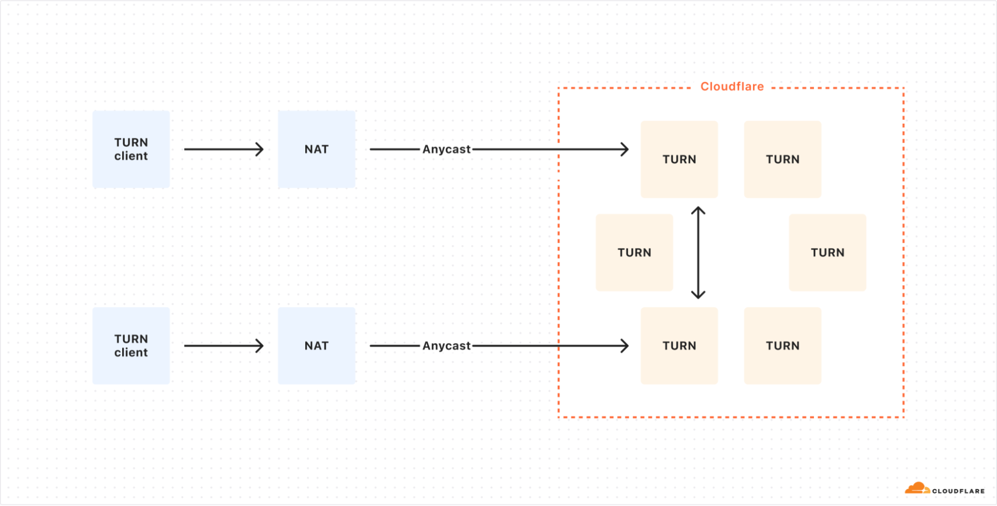
The optimized setup uses Anycast for all TURN clients, allowing for dynamic load distribution across Cloudflare’s globally distributed TURN servers.
Try Cloudflare Calls TURN today
The new TURN feature of Cloudflare Calls addresses critical challenges in real-time communication:
Connectivity: By solving NAT traversal issues, TURN ensures reliable connections even in complex network environments.
Privacy: Acting as an intermediary, TURN enhances user privacy by masking IP addresses and network details.
Performance: Leveraging Cloudflare’s global anycast network, our TURN service offers unparalleled speed and near-zero latency.
Scalability: With presence in over 330 cities, Cloudflare Calls TURN grows with your needs.
Cloudflare Calls TURN service is billed on a usage basis. It is available to self-serve and Enterprise customers alike. There is no cost for the first 1,000 GB (one terabyte) of Cloudflare Calls usage each month. It costs five cents per GB after your first terabyte of usage on self-serve. Volume pricing is available for Enterprise customers through your account team.
Switching TURN providers is likely as simple as changing a single configuration in your real-time app. To get started with Cloudflare’s TURN service, create a TURN app from your Cloudflare Calls Dashboard or read the Developer Docs.
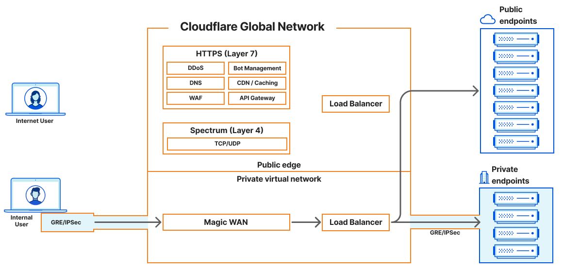
In 2023, Cloudflare introduced a new load balancing solution supporting Local Traffic Management (LTM). This year, we took it a step further by introducing support for layer 4 load balancing to private networks via Spectrum. Now, organizations can seamlessly balance public HTTP(S), TCP, and UDP traffic to their privately hosted applications. Today, we’re thrilled to unveil our latest enhancement: support for end-to-end private traffic flows as well as WARP authenticated device traffic, eliminating the need for dedicated hardware load balancers! These groundbreaking features are powered by the enhanced integration of Cloudflare load balancing with our Cloudflare One platform, and are available to our enterprise customers. With this upgrade, our customers can now utilize Cloudflare load balancers for both public and private traffic directed at private networks.
Cloudflare Load Balancing today
Before discussing the new features, let’s review Cloudflare’s existing load balancing support and the challenges customers face.
Cloudflare currently supports four main load balancing traffic flows:
Internet-facing load balancers connecting to publicly accessible endpoints at layer 7, supporting HTTP(S).
Internet-facing load balancers connecting to publicly accessible endpoints at layer 4 (Spectrum), supporting TCP and UDP services
Internet-facing load balancers connecting to private endpoints at layer 7 HTTP(S) via Cloudflare Tunnels.
Internet-facing load balancers connecting to private endpoints at layer 4 (Spectrum), supporting TCP and UDP services via Cloudflare Tunnels.
One of the biggest advantages of Cloudflare’s load balancing solutions is the elimination of hardware costs and maintenance. Unlike hardware-based load balancers, which are costly to purchase, license, operate, and upgrade, Cloudflare’s solution requires no hardware. There’s no need to buy additional modules or new licenses, and you won’t face end-of-life issues with equipment that necessitate costly replacements.
With Cloudflare, you can focus on innovation and growth. Load balancers are deployed in every Cloudflare data center across the globe, in over 300 cities, providing virtually unlimited scale and capacity. You never need to worry about bandwidth constraints, deployment locations, extra hardware modules, downtime, upgrades, or supply chain constraints. Cloudflare’s global Anycast network ensures that every customer connects to a nearby data center and load balancer, where policies, rules, and steering are applied efficiently. And now, the resilience, scale, and simplicity of Cloudflare load balancers can be integrated into your private networks! We have worked hard to ensure that Cloudflare load balancers are highly available and disaster ready, from the core to the edge – even when datacenters lose power.
Keeping private resources private with Magic WAN
Before today’s announcement, all of Cloudflare’s load balancers operating at layer 4 have been connected to the public Internet. Customers have been able to secure the traffic flowing to their load balancers with WAF rules and Zero Trust policies, but some customers would prefer to keep certain resources private and under no circumstances exposed to the Internet. It’s been possible to isolate origin servers and endpoints this way, which can exist on private networks that are only accessible via Cloudflare Tunnels. And as of today, we can offer a similar level of isolation to customers’ layer 4 load balancers.
In our previous LTM blog post, we discussed connecting these internal or private resources to the Cloudflare global network and how Cloudflare would soon introduce load balancers that are accessible via private IP addresses. Unlike other Cloudflare load balancers, these do not have an associated hostname. Rather, they are accessible via an RFC 1918 private IP address. In the land of load balancers, this is often referred to as a virtual IP (VIP). As of today, load balancers that are accessible at private IPs can now be used within a virtual network to isolate traffic to a certain set of Cloudflare tunnels, enabling customers to load balance traffic within their private network without exposing applications to the public Internet.
The question you might be asking is, “If I have a private IP load balancer and privately hosted applications, how do I or my users actually reach these now-private services?”
Cloudflare Magic WAN can now be used as an on-ramp in tandem with Cloudflare load balancers that are accessible via an assigned private IP address. Magic WAN provides a secure and high-performance connection to internal resources, ensuring that traffic remains private and optimized across our global network. With Magic WAN, customers can connect their corporate networks directly to Cloudflare’s global network with GRE or IPSec tunnels, maintaining privacy and security while enjoying seamless connectivity. The Magic WAN Connector easily establishes connectivity to Cloudflare without the need to configure network gear, and it can be deployed at any physical or cloud location! With the enhancements to Cloudflare’s load balancing solution, customers can confidently keep their corporate applications resilient while maintaining the end-to-end privacy and security of their resources.
This enhancement opens up numerous use cases for internal load balancing, such as managing traffic between different data centers, efficiently routing traffic for internally hosted applications, optimizing resource allocation for critical applications, and ensuring high availability for internal services. Organizations can now replace traditional hardware-based load balancers, reducing complexity and lowering costs associated with maintaining physical infrastructure. By leveraging Cloudflare load balancing and Magic WAN, companies can achieve greater flexibility and scalability, adapting quickly to changing network demands without the need for additional hardware investments.
But what about latency? Load balancing is all about keeping your applications resilient and performant and Cloudflare was built with speed at its core. There is a Cloudflare datacenter within 50ms of 95% of the Internet-connected population globally! Now, we support all Cloudflare One on-ramps to not only provide seamless and secure connectivity, but also to dramatically reduce latency compared to legacy solutions. Load balancing also works seamlessly with Argo Smart Routing to intelligently route around network congestion to improve your application performance by up to 30%! Check out the blogs here and here to read more about how Cloudflare One can reduce application latency.
Supporting distributed users with Cloudflare WARP
But what about when users are distributed and not connected to the local corporate network? Cloudflare WARP can now be used as an on-ramp to reach Cloudflare load balancers that are configured with private IP addresses. The Cloudflare WARP client allows you to protect corporate devices by securely and privately sending traffic from those devices to Cloudflare’s global network, where Cloudflare Gateway can apply advanced web filtering. The WARP client also makes it possible to apply advanced Zero Trust policies that check a device’s health before it connects to corporate applications.
In this load balancing use case, WARP pairs up perfectly with Cloudflare Tunnels so that customers can place their private origins within virtual networks to help either isolate traffic or handle overlapping private IP addresses. Once these virtual networks are defined, administrators can configure WARP profiles to allow their users to connect to the proper virtual networks. Once connected, WARP takes the configuration of the virtual networks and installs routes on the end users’ devices. These routes will tell the end user’s device how to reach the Cloudflare load balancer that was created with a private, non-publicly routable IP address. The administrator could then create a DNS record locally that would point to that private IP address. Once DNS resolves locally, the device would route all subsequent traffic over the WARP connection. This is all seamless to the user and occurs with minimal latency.
How we connected load balancing to Cloudflare One
In contrast to public L4 or L7 load balancers, private L4 load balancers are not going to have publicly addressable hostnames or IP addresses, but we still need to be able to handle their traffic. To make this possible, we had to integrate existing load balancing services with private networking services created by our Cloudflare One team. To do this, upon creation of a private load balancer, we now assign a private IP address within the customer’s virtual network. When traffic destined for a private load balancer enters Cloudflare, our private networking services make a request to load balancing to determine which endpoint to connect to. The information in the response from load balancing is used to connect directly to a privately hosted endpoint via a variety of secure traffic off-ramps. This differs significantly from our public load balancers where traffic is off-ramped to the public internet. In fact, we can now direct traffic from any on-ramp to any off-ramp! This allows for significant flexibility in architecture. For example, not only can we direct WARP traffic to an endpoint connected via GRE or IPSec, but we can also off-ramp this traffic to Cloudflare Tunnel, a CNI connection, or out to the public internet! Now, instead of purchasing a bespoke load balancing solution for each traffic type, like an application or network load balancer, you can configure a single load balancing solution to handle virtually any permutation of traffic that your business needs to run!
Getting started with internal load balancing
We are excited to be releasing these new load balancing features that solve critical connectivity issues for our customers and effectively eliminate the need for a hardware load balancer. Cloudflare load balancers now support end-to-end private traffic flows with Cloudflare One. To get started with configuring this feature, take a look at our load balancing documentation.
We are just getting started with our local traffic management load balancing support. There is so much more to come including user experience changes, enhanced layer 4 session affinity, new steering methods, refined control of egress ports, and more.
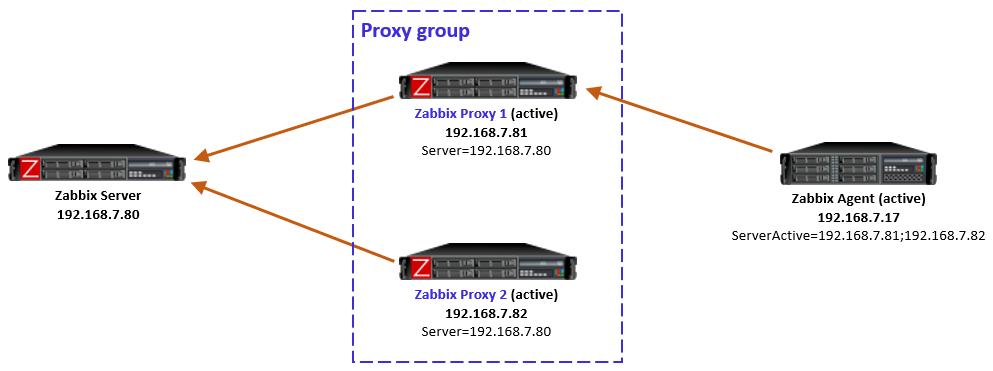
One of the new features in Zabbix 7.0 LTS is proxy load balancing. As the documentation says:
Proxy load balancing allows monitoring hosts by a proxy group with automated distribution of hosts between proxies and high proxy availability.
If one proxy from the proxy group goes offline, its hosts will be immediately distributed among other proxies having the least assigned hosts in the group.
Table of Contents
Proxy group is the new construct that enables Zabbix server to make dynamic decisions about the monitoring responsibilities within the group(s) of proxies. As you can see in the documentation, the proxy group has only a minimal set of configurable settings.
One important background information to understand is that Zabbix server always knows (within reasonable timeframe) which proxies in the proxy groups are online and which are not. That’s because all active proxies connect to the Zabbix server every 1 second by default (DataSenderFrequency setting in the proxy), and Zabbix server connects to the passive proxies also every 1 second by default (ProxyDataFrequency setting in the server), so if those connections are not happening anymore, then something is wrong with using the proxy.
Initially Zabbix server will balance the hosts between the proxies in the proxy group. It can also rebalance the hosts later if needed, the algorithm is described in the documentation. That’s something we don’t need to configure (that’s the “automated distribution of hosts” mentioned above). The idea is that, at any given time, any host configured to be monitored by the proxy group is monitored by one proxy only.
Now let’s see how the actual connections work with active and passive Zabbix agents. The active/passive modes of the proxies (with the Zabbix server connectivity) don’t matter in this context, but I’m using active proxies in my tests for simplicity.
Disclaimer: These are my own observations from my own Zabbix setup using 7.0.0, and they are not necessarily based on any official Zabbix documentation. I’m open for any comments or corrections in any case.
At the very end of this post I have included samples of captured agent traffic for each of the cases mentioned below.
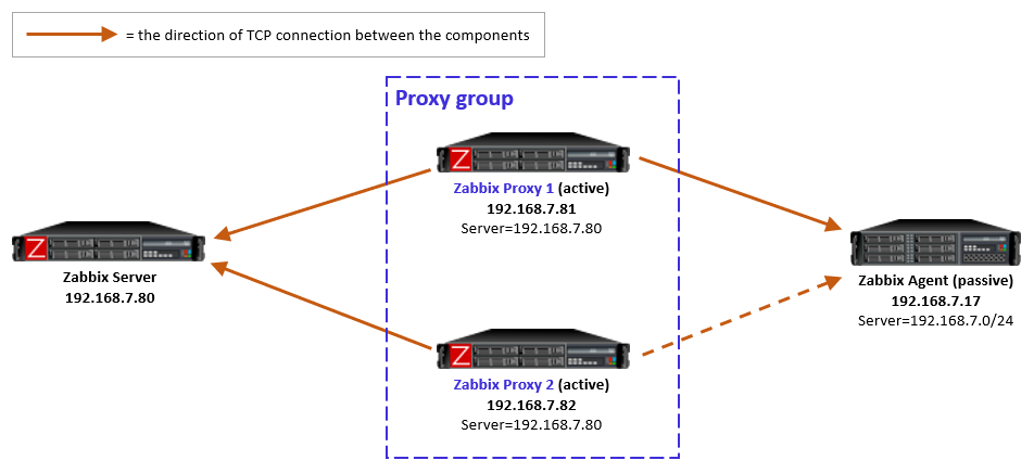
Passive agents monitored by a proxy group
For passive agents the proxy load balancing really is this simple: Whenever a proxy goes down in a proxy group, all the hosts that were previously monitored by that proxy will then be monitored by the other available proxies in the same proxy group.
There is nothing new to configure in the passive agents, only the usual Server directive to allow specific proxies (IP addresses, DNS names, subnets) to communicate with the agent.
As a reminder, a passive agent means that it listens to incoming requests from Zabbix proxies (or the Zabbix server), and then collects and returns the requested data. All relevant firewalls also need to be configured to allow the connections from the Zabbix proxies to the agent TCP port 10050.
As yet another reminder, each agent (or monitored host) can have both passive and active items configured, which means that it will both listen to incoming Zabbix requests but also actively request any active tasks from Zabbix proxies or servers. But again, this is long-existing functionality, nothing new in Zabbix 7.0.
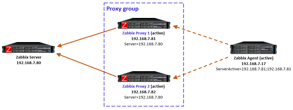
Active agents monitored by a proxy group
For active agents the proxy load balancing needs a bit new tweaking in the agent side.
By definition, an active agent is the party that initiates the connection to the Zabbix proxy (or server), to TCP port 10051 by default. The configuration happens with the ServerActive directive in the agent configuration. According to the official documentation, providing multiple comma-separated addresses in the ServerActive directive has been possible for ages, but it is for the purpose of providing data to multiple independent Zabbix installations at the same time. (Think about a Zabbix agent on a monitored host, being monitored by both a service provider and the inhouse IT department.)
Using semicolon-separated server addresses in ServerActive directive has been possible since Zabbix 6.0 when Zabbix servers are configured in high-availability cluster. That requires specific Zabbix server database implementation so that all the cluster nodes use the same database, and some other shared configurations.
Now in Zabbix 7.0 this same configuration style can be used for the agent to connect to all proxies in the proxy group, by entering all the proxy addresses in the ServerActive configuration, semicolon-separated. However, to be exact, this is not described in the ServerActive documentation as of this writing. Rather, it specifically says “More than one Zabbix proxy should not be specified from each Zabbix server/cluster.” But it works, let’s see how.
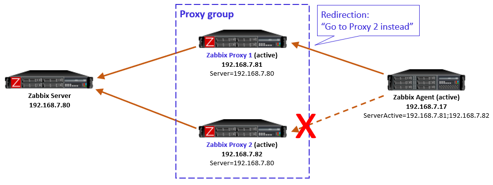
Using multiple semicolon-separated proxy addresses works because of the new redirection functionality in the proxy-agent communication: Whenever an active agent sends a message to a proxy, the proxy tells the agent to connect to another proxy, if the agent is currently assigned to some other proxy. The agent then ceases connecting to that previous proxy, and starts using the proxy address provided in the redirection instead. Thus the agent converges to using only that one designated proxy address.
In this simple example the Zabbix server determined that the agent should be monitored by Proxy 1, so when the agent initially contacted Proxy 1 (because its IP address is first in the ServerActive list), the proxy responded normally and agent was happy with that.
In case the Zabbix server had for any reason determined that the agent should be monitored by Proxy 2, then Proxy 1 would have responded with a redirection, and agent would have followed that. (There will be examples of redirections in the capture files below.)
To be clear, this agent redirection from the proxy group works only with Zabbix 7.0 agents as of this writing.
Note: In the initial version of this post I used comma-separated proxy addresses in ServerActive (instead of semicolon-separated), and that caused duplicate connections from the agent to the designated proxy (because the agent is not equipped to recognize that it connects to the same proxy twice), eventually causing data duplication in Zabbix database. Using comma-separated proxy addresses is thus not a working solution for proxy load balancing usage.
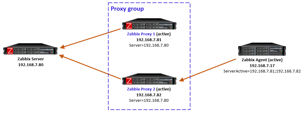
If the host-proxy assignments are changed by the Zabbix server for balancing the load between the proxies, the previously designated proxy will redirect the agent to the correct proxy address, and the situation is optimized again.
Side note: When configuring the proxies in Zabbix UI, there is a new Address for active agents field. That is the address value that is used by the proxies when responding with redirection messages to agents.
Proxy group failure scenarios with active agents
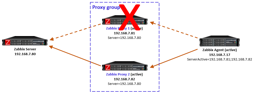
Proxy goes down
If the designated proxy of an active agent goes offline so that it doesn’t respond to the agent anymore, agent realizes the situation, discards the redirection information it had, and reverts to using the proxy addresses from ServerActive directive again.
Now, this is an interesting case because of some timing dependencies. In the proxy group configuration there is the Failover period configuration that controls the Zabbix server’s sensitivity to proxy availability in regards to agent rebalancing within the proxy group. Thus, if the agent reverts to using the other proxies faster than Zabbix server recognizes the situation and notifies the other proxies in the proxy group, the agent will get redirection responses from the other proxies, telling it to use the currently offline proxy. And the same happens again: agent fails to connect to the redirected proxy, and reverts to using the other locally configured proxies, and so on.
In my tests this looping was not very intense, only two rounds every second, so it was not very significant network-wise, and the situation will converge automatically when the Zabbix server has notified the proxies about the host rebalancing.
So this temporary looping is not a big deal. The takeaway is that the whole system converges automatically from a failed proxy.
After the failed proxy has recovered to online mode, the agents stay with their designated proxies in the proxy group.
As mentioned in the beginning, Zabbix server will automatically rebalance the hosts again after some time if needed.
Proxy is online but unreachable from the active agent
Another interesting case is one where the proxy itself is running and communicating with Zabbix server, thus being in online mode in the proxy group, but the active agent is not able to reach it, while still being able to connect to the other proxies in the group. This can happen due to various Internet-related routing issues for example, if the proxies are geographically distributed and far away from the agent.
Let’s start with the situation where the agent is currently monitored by Proxy 2 (as per the last picture above). When the failure starts and agent realizes that the connections to Proxy 2 are not succeeding anymore, the agent reverts to using the configured proxies in ServerActive, connecting to Proxy 1.
But, Proxy 1 knows (by the information given by Zabbix server) that Proxy 2 is still online and that the agent should be monitored by Proxy 2, so Proxy 1 responds to the agent with a redirection.
Obviously that won’t work for the agent as it doesn’t have connectivity to Proxy 2 anymore.
This is a non-recoverable situation (at least with the current Zabbix 7.0.0) while the reachability issue persists: The agent keeps on contacting Proxy 1, keeps receiving the redirection, and the same repeats over and over again.
Note that it does not matter if the agent is now locally reconfigured to only use Proxy 1 in this situation, because the load balancing of the hosts in the proxy group is not controlled by any of the agent-local configuration. The proxy group (led by Zabbix server) has the only authority to assign the hosts to the proxies.
One way to escape from this situation is to stop the unreachable Proxy 2. That way the Zabbix server will eventually notice that Proxy 2 is offline, and the hosts will be automatically rebalanced to other proxies in the group, thus removing the agent-side redirection to the unreachable proxy.
Keep this potential scenario in mind when planning proxy groups with proxy location diversity.
This is also something to think about if your Zabbix proxies have multiple network interfaces, where Zabbix server connectivity is using different interface from the agent connectivity. In that case the same problem can occur due to your own configurations.
Closing words
All in all, proxy load balancing looks very promising feature as it does not require any network-level tricks to achieve load balancing and high availability. In Zabbix 7.0 this is a new feature, so we can expect some further development for the details and behavior in the upcoming releases.
Appendix: Sample capture files
Ideally these capture files should be viewed with Wireshark version 4.3.0rc1 or newer because only the latest Wireshark builds include support for latest Zabbix protocol features. Wireshark 4.2.x should also show most of the Zabbix packet fields. Use display filter “zabbix” to see only the Zabbix protocol packets, but when examining cases more carefully you should also check the plain TCP packets (without any display filter) to get more understanding about the cases.
These samples are taken with Zabbix components version 7.0.0, using default timers in the Zabbix process configurations, and 20 seconds as the proxy group failover period.
Agent connected to Proxy 2, but Proxy 2 keeps sending redirects
Proxy 2 was assigned the agent before frame #1074, so it took over the monitoring and accepted the agent connections
Proxy 1 was later restarted (but agent didn’t try to connect to it yet)
The agent was manually restarted before frame #1498 and it connected to Proxy 1 again, was given a redirection to Proxy 2, and continued with Proxy 2 again
In 2023, Cloudflare introduced a new load balancing solution, supporting Local Traffic Management (LTM). This gives organizations a way to balance HTTP(S) traffic between private or internal servers within a region-specific data center. Today, we are thrilled to be able to extend those same LTM capabilities to non-HTTP(S) traffic. This new feature is enabled by the integration of Cloudflare Spectrum, Cloudflare Tunnels, and Cloudflare load balancers and is available to enterprise customers. Our customers can now use Cloudflare load balancers for all TCP and UDP traffic destined for private IP addresses, eliminating the need for expensive on-premise load balancers.
A quick primer
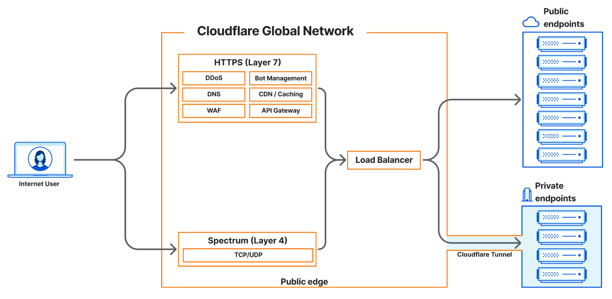
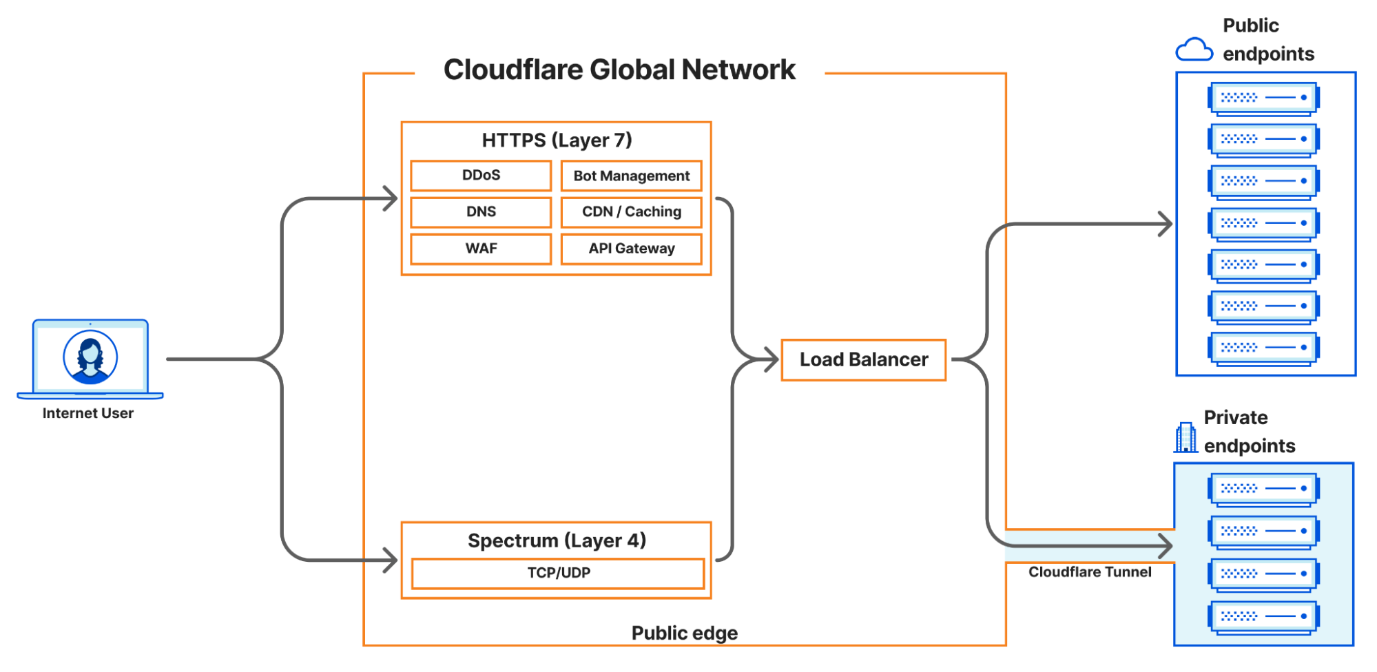
In this blog post, we will be referring to load balancers at either layer 4 or layer 7. This is, of course, referring to layers of the OSI model but more specifically, the ingress path that is being used to reach the load balancer. Layer 7, also known as the Application Layer, is where the HTTP(S) protocol exists. Cloudflare is well known for our layer 7 capabilities, which are built around speeding up and protecting websites which run over HTTP(S). When we refer to layer 7 load balancers, we are referring to HTTP(S)-based services. Our layer 7 stack allows Cloudflare to apply services like CDN, WAF, Bot Management, DDoS protection, and more to a customer’s website or application to improve performance, availability, and security.
Layer 4 load balancers operate at a lower level of the OSI model, called the Transport Layer, which means they can be used to support a much broader set of services and protocols. At Cloudflare, our public layer 4 load balancers are enabled by a Cloudflare product called Spectrum. Spectrum works as a layer 4 reverse proxy. This places Cloudflare in front of any DDoS attacks that may be launched against Spectrum-proxied services, and by using Spectrum in front of your application, your private origin IP address is concealed, which also prevents bad actors from discovering and attacking your origin’s IP address directly.
Services that use TCP or UDP for transport can leverage Spectrum with a Cloudflare load balancer. Layer 4 load balancing allows us to support other application layer protocols such as SSH, FTP, NTP, and SMTP since they operate over TCP and UDP. Given the breadth of services and protocols this represents, the treatment provided is more generalized. Cloudflare Spectrum supports features such as TLS/SSL offloading, DDoS protection, Argo Smart Routing, and session persistence with our layer 4 load balancers.
Cloudflare’s current load balancing capabilities
Before we dig into the new features we are announcing, it’s important to understand what Cloudflare load balancing supports today and the challenges our customers face with regard to their load balancing needs.
There are three main load balancing traffic flows that Cloudflare supports today:
Internet-facing load balancers connecting to publicly accessible origins operating at layer 7, which supports HTTP(S)
Internet-facing load balancers connecting to publicly accessible origins operating at layer 4 (Spectrum), which supports all TCP-based and UDP-based services such as SSH, FTP, NTP, SMTP, etc.
Publicly accessible load balancers connecting to private origins operating at layer 7 HTTP(S) over Cloudflare Tunnels
One of the biggest advantages Cloudflare’s load balancing solutions offer our customers is that there is no hardware to purchase or maintain. Hardware-based load balancers are expensive to purchase, license, operate, and upgrade. “Need more bandwidth? Just buy and install this additional module.” “Need more features? Just buy and install this new license.” “Oh, your hardware load balancer is End-of-Life? Just purchase an entire new kit which we will EOL in a few years!” The upgrade or refresh cycle on a fully integrated LTM load balancer setup can take years and, by the time you finish the planning, implementation, and cutover, it might actually be time to start planning the next refresh.
Cloudflare eliminates all these concerns and lets you focus on innovation and growth. Your load balancers exist in every Cloudflare data center across the globe, in over 300 cities, with virtually unlimited scale and capacity. You never need to worry about bandwidth constraints, deployment locations, extra hardware modules, downtime, upgrades, or maintenance windows ever again. With Cloudflare’s global Anycast network, every customer connects to a nearby Cloudflare data center and load balancer, where relevant policies, rules, and steering are applied.
Load balancing more than websites with Cloudflare Spectrum
Today, we are excited to announce that Cloudflare Spectrum can now support load balancing traffic to private networks. The addition of private IP origin support for Cloudflare load balancers is very powerful and that’s why we are extending that support to load balancing with Cloudflare Spectrum as well. This means that any set of private or internal applications that use TCP or UDP can now be locally load balanced via Cloudflare. These services will also benefit from Spectrum’s layer 3/4 DDoS protection and can leverage other features like session persistence without compromising security. So while the ingress to these load balancers is public, the origins to which they distribute traffic can all be private, inaccessible from the public Internet.
Ordinarily, load balancing to private networks would require expensive on-premise hardware or costly direct physical connections to cloud providers. But, by using Spectrum as the ingress path for TCP and UDP load balancing, customers can keep their origins completely protected and unreachable from the Internet and allow access exclusively through their Cloudflare load balancer – no expensive hardware required. Customers no longer need to manage complex ACLs or security settings to make sure only certain source IP addresses are connecting to the origins. These private origins can be hosted in private data centers, a public cloud, a private cloud, or on-premise.
How we enabled Spectrum to support private networks
All of our changes to create this feature center around integrations with Apollo, the unifying service created by the Cloudflare Zero Trust team. You can read their previous blog post on the Oxy framework for more details on how Zero Trust handles and routes traffic. Apollo accepts incoming traffic from supported on-ramps, applies Zero Trust logic as configured by the customer, and then routes the traffic to egress via supported off-ramps. For example, Apollo enables clients connected securely using Cloudflare’s WARP client to communicate over Cloudflare Tunnels with private origins in a customer’s data center. Now, Apollo is being extended to do more.
When a user creates a load balanced Spectrum app, they choose a hostname and port, and select a Cloudflare load balancer as their origin. This allocates a hostname which will resolve to an IP address where Spectrum will listen for incoming traffic on the customer-configured port. Spectrum makes a call to Cloudflare’s internal load balancing service, Director, which responds with the appropriate endpoint, to which Spectrum will proxy the connection. Previously, load balanced Spectrum apps only supported publicly addressable origins. Now, if the response from Director indicates that the traffic is destined for a private origin, Spectrum passes the private origin’s IP address and virtual network ID to Apollo, which then proxies the traffic to the customer’s private origin.
In short, new integrations between our Spectrum service and Apollo and between Apollo and Director have allowed us to expand our load balancing offerings not only to layer 4, but also enable us to leverage virtual networks to keep load balanced traffic private and off the public Internet. This also sets the stage for integrating load balancing with other traffic on-ramps and off-ramps, such as WARP, in the future. It also opens the door to a number of exciting possibilities like load balancing authenticated device traffic to private networks or even load balancing internal traffic that is never exposed to the public Internet.
Looking to the future
We are excited to be releasing this new load balancing feature which enables Cloudflare Spectrum to reach private IP endpoints. Cloudflare load balancers now support steering any TCP or UDP-based protocols over Cloudflare Tunnels to private IP endpoints, which are otherwise not accessible via the public Internet. You can learn more about how to configure this feature on our load balancing documentation pages.
We are just getting started with our local traffic management load balancing support. There is so much more to come including support for load balancing internal traffic, enhanced layer 4 session affinity, new steering methods, additional traffic ingress methods, and more!
In the dynamic world of modern applications, efficient load balancing plays a pivotal role in delivering exceptional user experiences. Customers commonly leverage load balancing, so they can efficiently use their existing infrastructure resources in the best way possible. Though, load balancing is not a ‘one-size-fits-all, out of the box’ solution for everyone. As you go deeper into the details of your traffic shaping requirements and as your architecture becomes more complex, different flavors of load balancing are usually required to achieve these varying goals, such as steering between datacenters for public traffic, creating high availability for critical internal services with private IPs, applying steering between servers in a single datacenter, and more. We are extremely excited to announce a new addition to our Load Balancing solution, Local Traffic Management (LTM) with deep integrations with Zero Trust!
A common problem businesses run into is that almost no providers can satisfy all these requirements, resulting in a growing list of vendors to manage disparate data sources to get a clear view of your traffic pipeline, and investment into incredibly expensive hardware that is complicated to set up and maintain. Not having a single source of truth to dwindle down ‘time to resolution’ and a single partner to work with in times when things are not operating within the ideal path can be the difference between a proactive, healthy growing business versus one that is reactive and constantly having to put out fires. The latter can result in extreme slowdown to developing amazing features/services, reduction in revenue, tarnishing of brand trust, decreases in adoption – the list goes on!
For eight years, we have provided top-tier global traffic load balancing (GTM) capabilities to thousands of customers across the globe. But why should the steering intelligence, failover, and reliability we guarantee stop at the front door of the selected datacenter and only operate with public traffic? We came to the conclusion that we should go even further. Today is the start of a long series of new features that allow traffic steering, failover, session persistence, SSL/TLS offloading and much more to take place between servers after datacenter selection has occurred! Instead of relying only on the relative weight to determine which server traffic should be sent to, you can now bring the same intelligent steering policies, such as least outstanding requests steering or hash steering, to any of your many data centers. This also means you have a single partner for all of your load balancing initiatives and a single pane of glass to inform business decisions! Cloudflare is thrilled to introduce the powerful combination of private IP support for Load Balancing with Cloudflare Tunnels and Local Traffic Management, offering customers a solution that blends unparalleled efficiency, security, flexibility, and privacy.
What is a load balancer?
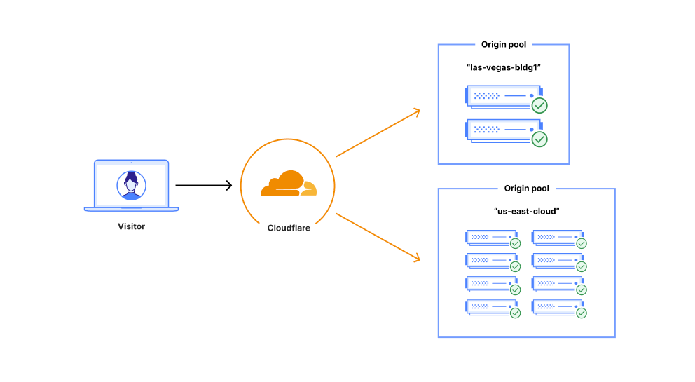
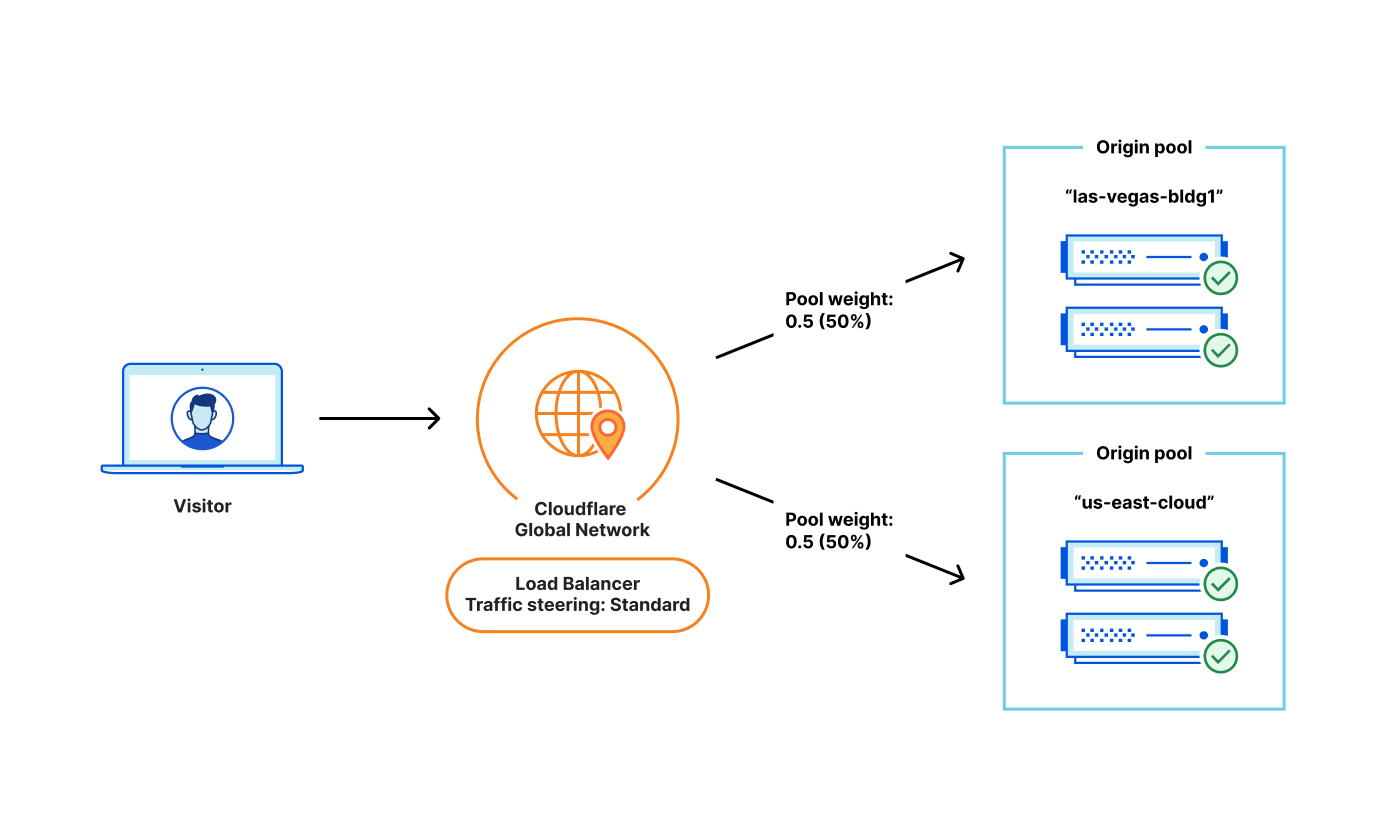
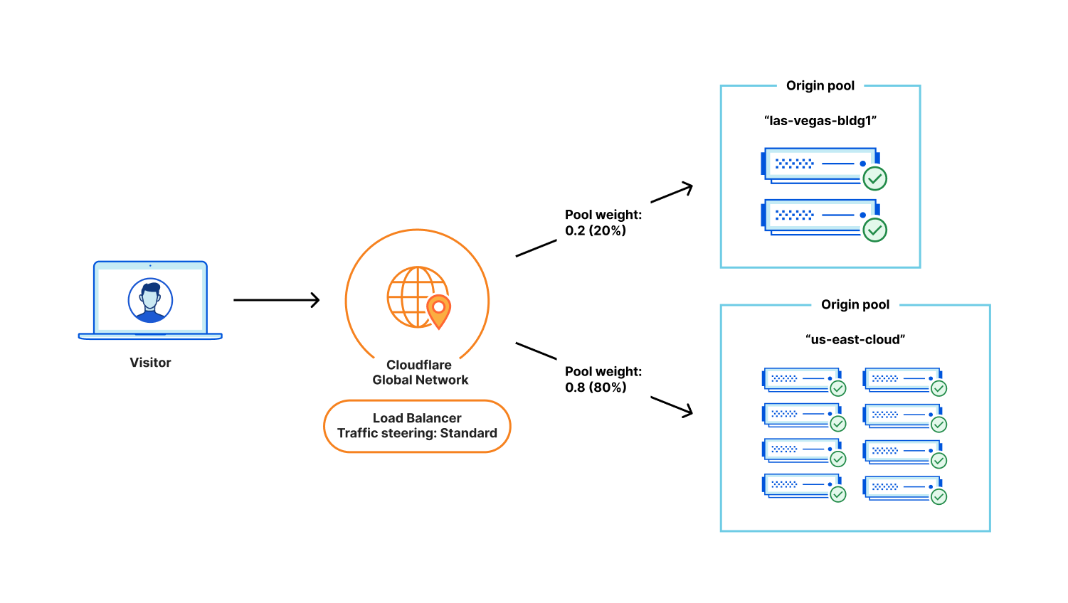
A Cloudflare load balancer directs a request from a user to the appropriate origin pool within a data center
Load balancing — functionality that’s been around for the last 30 years to help businesses leverage their existing infrastructure resources. Load balancing works by proactively steering traffic away from unhealthy origin servers and — for more advanced solutions — intelligently distributing traffic load based on different steering algorithms. This process ensures that errors aren’t served to end users and empowers businesses to tightly couple overall business objectives to their traffic behavior. Cloudflare Load Balancing has made it simpler and easier to securely and reliably manage your traffic across multiple data centers around the world. With Cloudflare Load Balancing, your traffic will be directed reliably regardless of the scale of traffic or where it originates with customizable steering, affinity and failover. This clearly has an advantage over a physical load balancer since it can be configured easily and traffic doesn’t have to reach one of your data centers to be routed to another location, introducing single points of failure and significant latency. When compared with other global traffic management load balancers, Cloudflare’s Load Balancing offering is easier to set up, simpler to understand, and is fully integrated with the Cloudflare platform as one single product for all load balancing needs.
What are Cloudflare Tunnels?
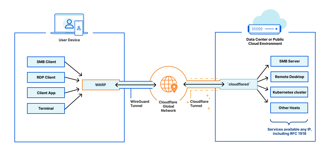
Origins and servers of various types can be connected to Cloudflare using Cloudflare Tunnel. Users can also secure their traffic using WARP, allowing traffic to be secured and managed end to end through Cloudflare.
In 2018, Cloudflare introduced Cloudflare Tunnels, a private, secure connection between your data center and Cloudflare. Traditionally, from the moment an Internet property is deployed, developers spend an exhaustive amount of time and energy locking it down through access control lists, rotating IP addresses, or more complex solutions like GRE tunnels. We built Tunnel to help alleviate that burden. With Tunnels, users can create a private link from their origin server directly to Cloudflare without exposing your services directly to the public internet or allowing incoming connections in your data center’s firewall. Instead, this private connection is established by running a lightweight daemon, cloudflared, in your data center, which creates a secure, outbound-only connection. This means that only traffic that you’ve configured to pass through Cloudflare can reach your private origin.
Unleashing the potential of Cloudflare Load Balancing with Cloudflare Tunnels
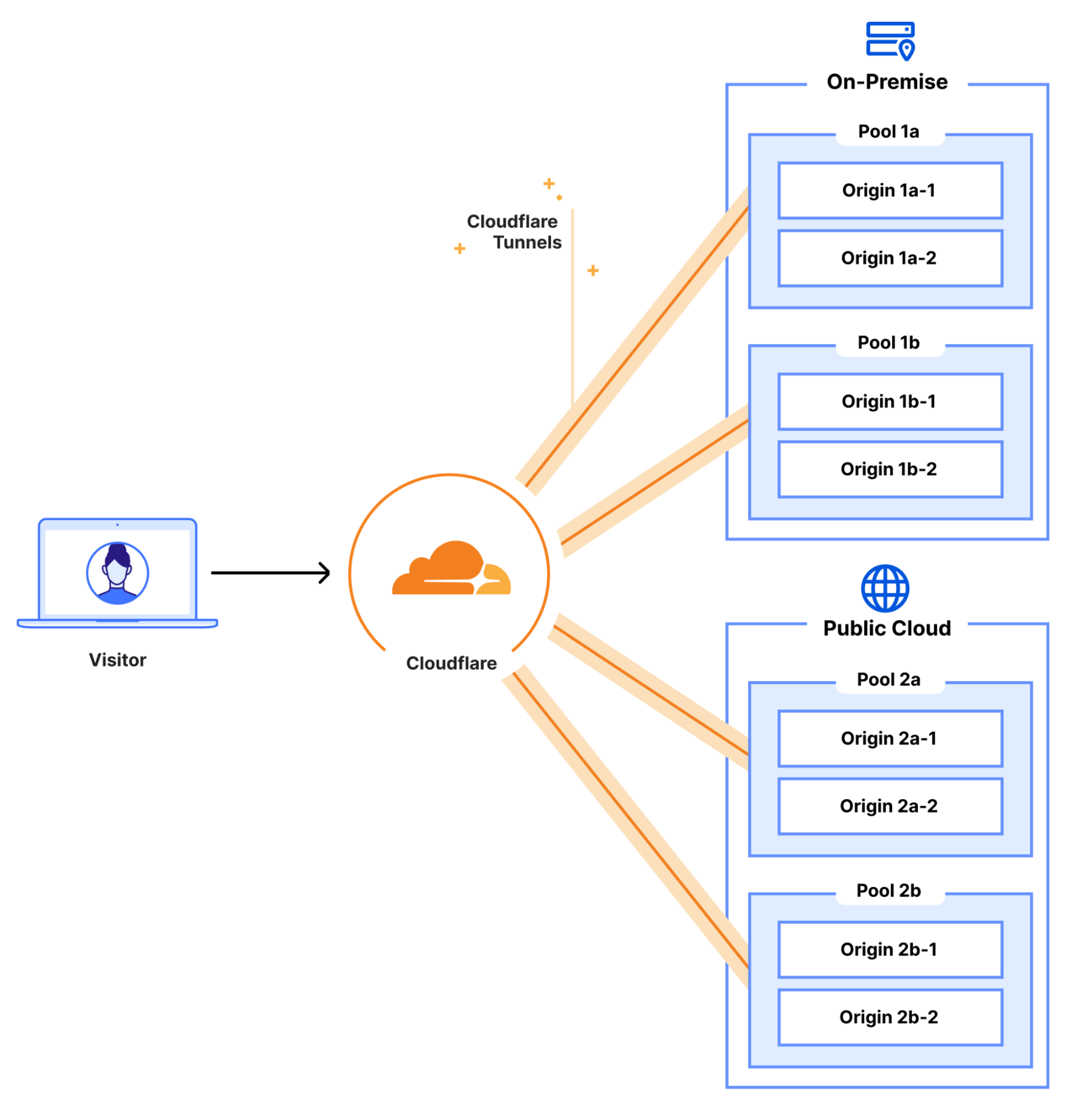
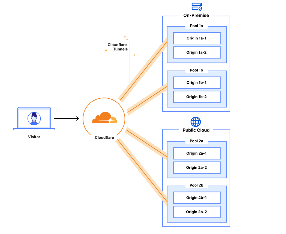
Cloudflare Load Balancing can easily and securely direct a user’s request to a specific origin within your private data center or public cloud using Cloudflare Tunnels
Combining Cloudflare Tunnels with Cloudflare Load Balancing allows you to remove your physical load balancers from your data center and have your Cloudflare load balancer reach out to your servers directly via their private IP addresses with health checks, steering, and all other Load Balancing features currently available. Instead of configuring your on-premise load balancer to expose each service and then updating your Cloudflare load balancer, you can configure it all in one place. This means that from the end-user to the server handling the request, all your configuration can be done in a single place – the Cloudflare dashboard. On top of this, you can say goodbye to the multi hundred thousand dollar price tag to hardware appliances, the incredible management overhead and investing in a solution that has a time limit for its delivered value.
Load Balancing serves as the backbone for online services, ensuring seamless traffic distribution across servers or data centers. Traditional load balancing techniques often require exposing services on a data center’s public IP addresses, forcing organizations to create complex configurations vulnerable to security risks and potential data exposure. By harnessing the power of private IP support for Load Balancing in conjunction with Cloudflare Tunnels, Cloudflare is revolutionizing the way businesses protect and optimize their applications. With clear steps to install the cloudflared agent to connect your private network to Cloudflare’s network via Cloudflare Tunnels, directly and securely routing traffic into your data centers becomes easier than ever before!
Publicly exposing services in private data centers is complicated
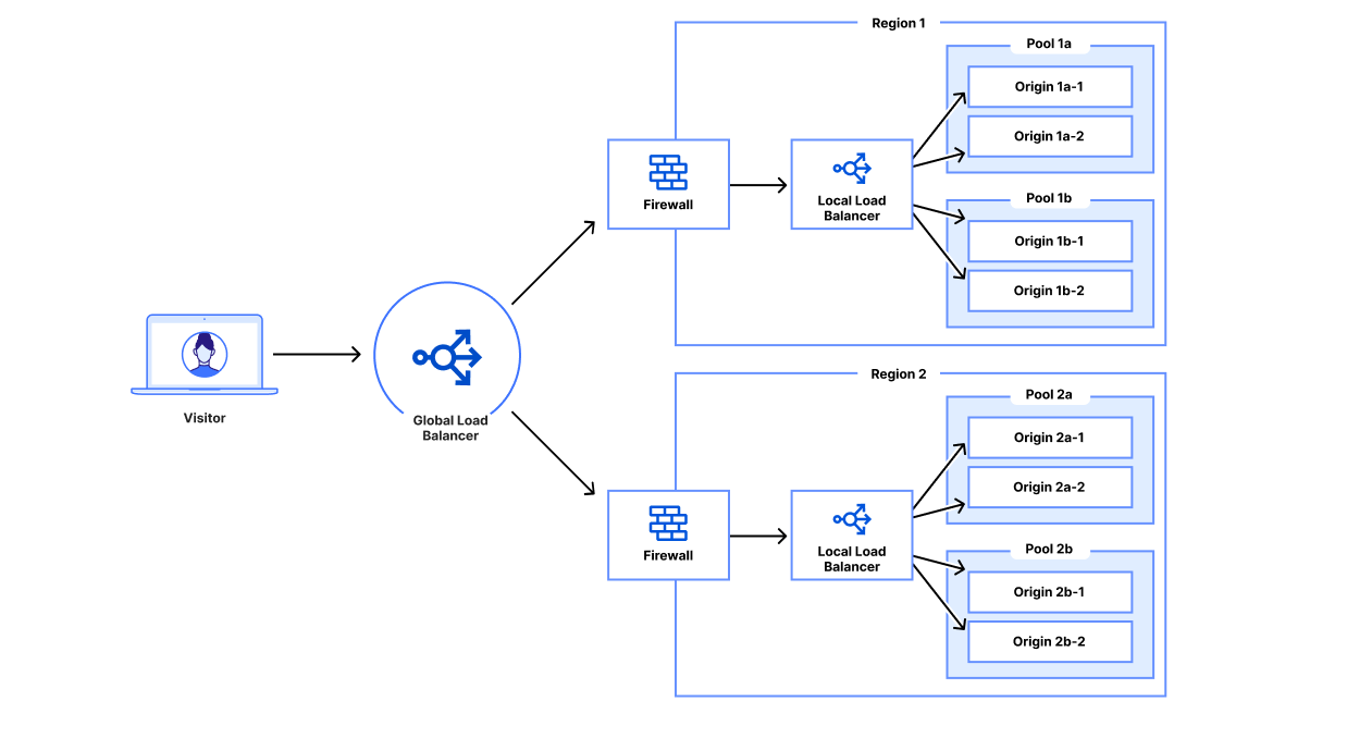
A visitor’s request hits a global traffic management (GTM) load balancer directing the request to a data center, then a firewall, then a local traffic management (LTM) load balancer and then an origin
Load balancing within a private data center can be expensive and difficult to manage. The idea of keeping security first while ensuring ease of use and flexibility for your internal workforce is a tricky balance to strike. It’s not only the ‘how’ of securely exposing internal services, but how to best balance traffic between servers at a single location within your private network!
In a private data center, even a very simple website can be fairly complex in terms of networking and configuration. Let’s walk through a simple example of a customer device connecting to a website. A customer device performs a DNS lookup for the business’s website and receives an IP address corresponding to a customer data center. The customer then makes an HTTPS request to that IP address, passing the original hostname via Server Name Indication (SNI). That load balancer forwards that request to the corresponding origin server and returns the response to the customer device.
This example doesn’t have any advanced functionality and the stack is already difficult to configure:
Expose the service or server on a private IP.
Configure your data center’s networking to expose the LB on a public IP or IP range.
Configure your load balancer to forward requests for that hostname and/or public IP to your server’s private IP.
Configure a DNS record for your domain to point to your load balancer’s public IP.
In large enterprises, each of these configuration changes likely requires approval from several stakeholders and modified through different repositories, websites and/or private web interfaces. Load balancer and networking configurations are often maintained as complex configuration files for Terraform, Chef, Puppet, Ansible or a similar infrastructure-as-code service. These configuration files can be syntax checked or tested but are rarely tested thoroughly prior to deployment. Each deployment environment is often unique enough that thorough testing is often not feasible given the time and hardware requirements needed to do so. This means that changes to these files can negatively affect other services within the data center. In addition, opening up an ingress to your data center widens the attack surface for varying security risks such as DDoS attacks or catastrophic data breaches. To make things worse, each vendor has a different interface or API for configuring their devices or services. For example, some registrars only have XML APIs while others have JSON REST APIs. Each device configuration may have different Terraform providers or Ansible playbooks. This results in complex configurations accumulating over time that are difficult to consolidate or standardize, inevitably resulting in technical debt.
Now let’s add additional origins. For each additional origin for our service, we’ll have to go set up and expose that origin and configure the physical load balancer to use our new origin. Now let’s add another data center. Now we need another solution to distribute across our data centers. This results in a separate global traffic management system and local traffic management system. These solutions have in the past come from different vendors and will have to be configured in different ways even though they should serve the same purpose: load balancing. This makes managing your web traffic unnecessarily difficult. Why should you have to configure your origins in two different load balancers? Why can’t you manage all the traffic for all the origins for a service in the same place?
Simpler and better: Load Balancing with Tunnels
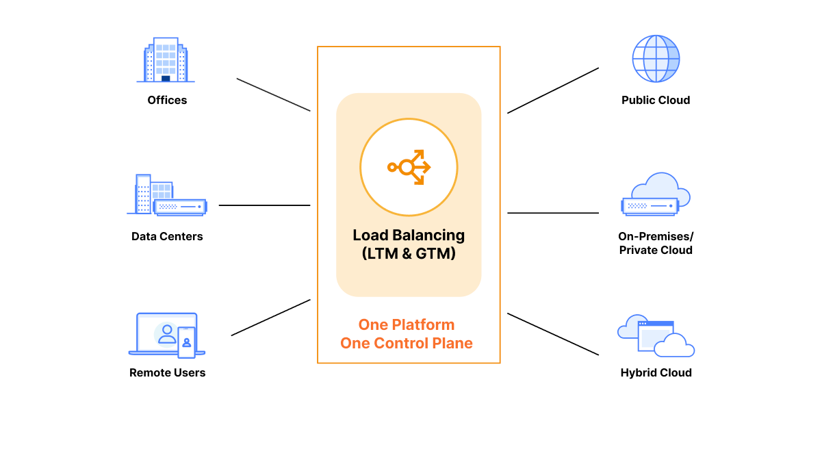
Cloudflare Load Balancing can manage traffic for all your offices, data centers, remote users, public clouds, private clouds and hybrid clouds in one place
With Cloudflare Load Balancing and Cloudflare Tunnel, you can manage all your public and private origins in one place: the Cloudflare dashboard. Cloudflare load balancers can be easily configured using the Cloudflare dashboard or the Cloudflare API. There’s no need to SSH or open a remote desktop to modify load balancer configurations for your public or private servers. All configurations can be done through the dashboard UI or Cloudflare API, with full parity between the two.
With Cloudflare Tunnel set up and running in your data center, everything is ready to connect your origin server to Cloudflare network and load balancers. You do not need to configure any ingress to your data center since Cloudflare Tunnel operates only over outbound connections and can securely reach out to privately addressed services inside your data center. To expose your service to Cloudflare, you just set up your private IP range to be routed over that tunnel. Then, you can create a Cloudflare load balancer and input the corresponding private IP address and virtual network ID into your origin pool. After that, Cloudflare manages the DNS and load balancing across your private servers. Now your origin is receiving traffic exclusively via Cloudflare Tunnel and your physical load balancer is no longer needed!
This groundbreaking integration enables organizations to deploy load balancers while keeping their applications securely shielded from the public Internet. The customer’s traffic passes through Cloudflare’s data centers, allowing customers to continue to take full advantage of Cloudflare’s security and performance services. Also, by leveraging Cloudflare Tunnels, traffic between Cloudflare and customer origins remains isolated within trusted networks, bolstering privacy, security, and peace of mind.
The advantages of Private IP support with Cloudflare Tunnels
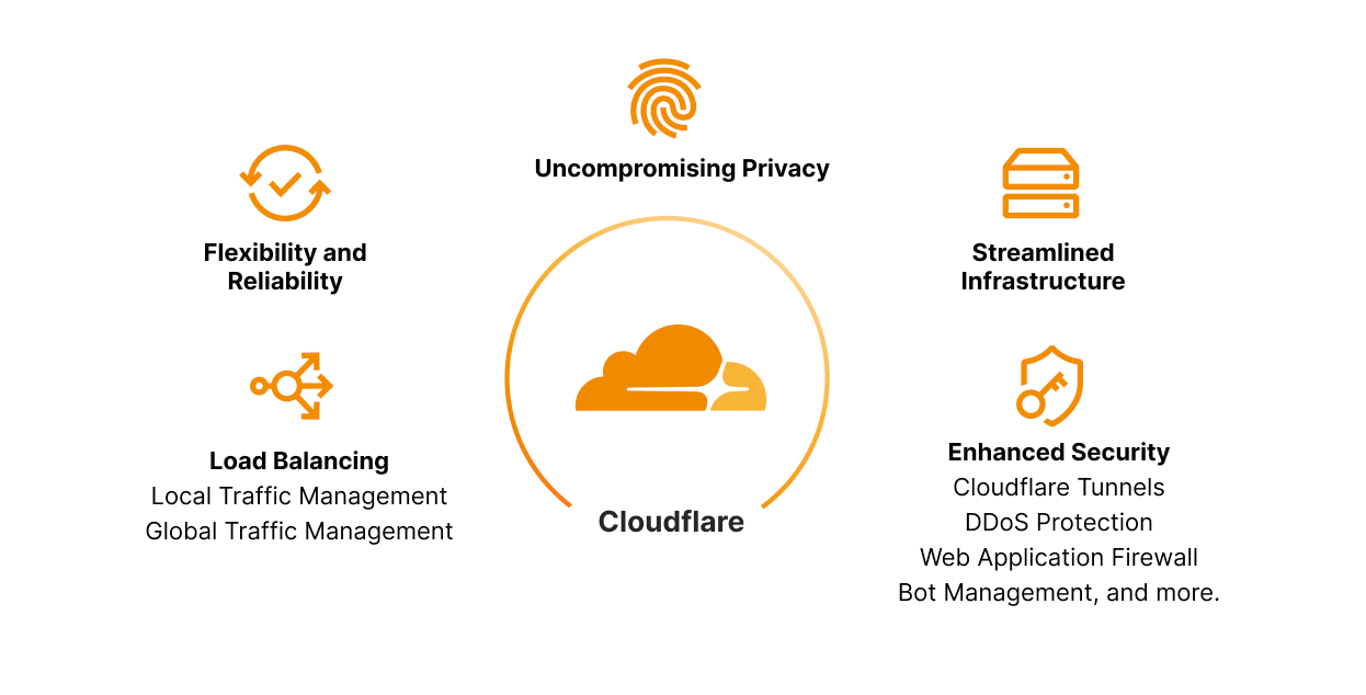
Cloudflare Load Balancing works in conjunction with all the security and privacy products that Cloudflare has to offer including DDoS protection, Web Application Firewall and Bot Managment
Combining Global and Local Traffic Management: All the features and ease of use that were part of Cloudflare Load Balancing for Global Traffic Management are also available with Local Traffic Management. You can configure your public and private origins in one dashboard as opposed to several services and vendors. Now, all your private origins can benefit from the features that Cloudflare Load Balancing is known for: instant failover, customizable steering between data centers, ease of use, custom rules and configuration updates in a matter of seconds. They will also benefit from our newer features including least connection steering, least outstanding request steering, and session affinity by header. This is just a small subset of the expansive feature set for Load Balancing. See our dev docs for more features and details on the offering.
Enhanced Security: By combining private IP support with Cloudflare Tunnels, organizations can fortify their security posture and protect sensitive data. With private IP addresses and encrypted connections via Cloudflare Tunnel, the risk of unauthorized access and potential attacks is significantly reduced – traffic remains within trusted networks. You can also configure Cloudflare Access to add single sign-on support for your application and restrict your application to a subset of authorized users. In addition, you still benefit from Firewall rules, Rate Limiting rules, Bot Management, DDoS protection and all the other Cloudflare products available today allowing comprehensive security configurations.
Uncompromising Privacy: As data privacy continues to take center stage, businesses must ensure the confidentiality of user information. Cloudflare's private IP support with Cloudflare Tunnels enables organizations to segregate applications and keep sensitive data within their private network boundaries. Custom rules also allow you to direct traffic for specific devices to specific data centers. For example, you can use custom rules to direct traffic from Eastern and Western Europe to your European data centers, so you can easily keep those users’ data within Europe. This minimizes the exposure of data to external entities, preserving user privacy and complying with strict privacy regulations across different geographies.
Flexibility & Reliability: Scale and adaptability are some of the major foundations of a well-operating business. Implementing solutions that fit your business’ needs today is not enough. Customers must find solutions that meet their needs for the next three or more years. The blend of Load Balancing with Cloudflare Tunnels within our Zero Trust solution lends to the very definition of flexibility and reliability! Changes to load balancer configurations propagate around the world in a matter of seconds, making load balancers an effective way to respond to incidents. Also, instant failover, health monitoring, and steering policies all help to maintain high availability for your applications, so you can deliver the reliability that your users expect. This is all in addition to best in class Zero Trust capabilities that are deeply integrated such as, but not limited to Secure Web Gateway (SWG), remote browser isolation, network logs. Data loss prevention.
Streamlined Infrastructure: Organizations can consolidate their network architecture and establish secure connections across distributed environments. This unification reduces complexity, lowers operational overhead, and facilitates efficient resource allocation. Whether you need to apply a global traffic manager to intelligently direct traffic between datacenters within your private network, or steer between specific servers after datacenter selection has taken place, there is now a clear, single lens to manage your global and local traffic, regardless of whether the source or destination of the traffic is public or private. Complexity can be a large hurdle in achieving and maintaining fast, agile business units. Consolidating into a single provider, like Cloudflare, that provides security, reliability, and observability will not only save significant cost but allows your teams to move faster and focus on growing their business, enhancing critical services, and developing incredible features, rather than taping together infrastructure that may not work in a few years. Leave the heavy lifting to us, and let us empower you and your team to focus on creating amazing experiences for your employees and end-users.
The lack of agility, flexibility, and lean operations of hardware appliances for Local Traffic Management does not justify the hundreds of thousands of dollars spent on them, along with the huge overhead of managing CPU, memory, power, cooling, etc. Instead, we want to help businesses move this logic to the cloud by abstracting away the needless overhead and bringing more focus back to teams to do what they do best, building amazing experiences, and allowing Cloudflare to do what we do best, protecting, accelerating, and building heightened reliability. Stay tuned for more updates on Cloudflare's Local Traffic Manager and how it can reduce architecture complexity while bringing more insight, security, and control to your teams. In the meantime, check out our new whitepaper!
Looking to the future
Cloudflare's impactful solution, private IP support for Load Balancing with Cloudflare Tunnels as part of the Zero Trust solution, reaffirms our commitment to providing cutting-edge tools that prioritize security, privacy, and performance. By leveraging private IP addresses and secure tunnels, Cloudflare empowers businesses to fortify their network infrastructure while ensuring compliance with regulatory requirements. With enhanced security, uncompromising privacy, and streamlined infrastructure, load balancing becomes a powerful driver of efficient and secure public or private services.
As a business grows and its systems scale up, they'll need the features that Cloudflare Load Balancing is known for: health monitoring, steering, and failover. As availability requirements increase due to growing demands and standards from end-users, customers can add health checks, enabling automatic failover to healthy servers when an unhealthy server begins to fail. When the business begins to receive more traffic from around the world, they can create new pools for different regions and use dynamic steering to reduce latency between the user and the server. For intensive or long-running requests, such as complex datastore queries, customers can benefit from leveraging least outstanding requests steering to reduce the number of concurrent requests per server. Before, this could all be done with publicly addressable IPs, but it is now available for pools with public IPs, private servers, or combinations of the two. Private IP Load Balancing along with Local Traffic Management is live and ready to use today! Check out our dev docs for instructions on how to get started.
Stay tuned for our next addition to add new Load Balancing onramp support for Spectrum and WARP with Cloudflare Tunnels with private IPs for your Layer 4 traffic, allowing us to support TCP and UDP applications in your private data centers!
When Zuul was designed and developed, there was an inherent assumption that connections were effectively free, given we weren’t using mutual TLS (mTLS). It’s built on top of Netty, using event loops for non-blocking execution of requests, one loop per core. To reduce contention among event loops, we created connection pools for each, keeping them completely independent. The result is that the entire request-response cycle happens on the same thread, significantly reducing context switching.
There is also a significant downside. It means that if each event loop has a connection pool that connects to every origin (our name for backend) server, there would be a multiplication of event loops by servers by Zuul instances. For example, a 16-core box connecting to an 800-server origin would have 12,800 connections. If the Zuul cluster has 100 instances, that’s 1,280,000 connections. That’s a significant amount and certainly more than is necessary relative to the traffic on most clusters.
As streaming has grown over the years, these numbers multiplied with bigger Zuul and origin clusters. More acutely, if a traffic spike occurs and Zuul instances scale up, it exponentially increases connections open to origins. Although this has been a known issue for a long time, it has never been a critical pain point until we moved large streaming applications to mTLS and our Envoy-based service mesh.
Fixing the Flows
The first step in improving connection overhead was implementing HTTP/2 (H2) multiplexing to the origins. Multiplexing allows the reuse of existing connections by creating multiple streams per connection, each able to send a request. Rather than requiring a connection for every request, we could reuse the same connection for many simultaneous requests. The more we reuse connections, the less overhead we have in establishing mTLS sessions with roundtrips, handshaking, and so on.
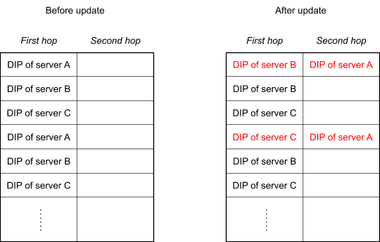
Although Zuul has had H2 proxying for some time, it never supported multiplexing. It effectively treated H2 connections as HTTP/1 (H1). For backward compatibility with existing H1 functionality, we modified the H2 connection bootstrap to create a stream and immediately release the connection back into the pool. Future requests will then be able to reuse the existing connection without creating a new one. Ideally, the connections to each origin server should converge towards 1 per event loop. It seems like a minor change, but it had to be seamlessly integrated into our existing metrics and connection bookkeeping.
The standard way to initiate H2 connections is, over TLS, via an upgrade with ALPN (Application-Layer Protocol Negotiation). ALPN allows us to gracefully downgrade back to H1 if the origin doesn’t support H2, so we can broadly enable it without impacting customers. Service mesh being available on many services made testing and rolling out this feature very easy because it enables ALPN by default. It meant that no work was required by service owners who were already on service mesh and mTLS.
Sadly, our plan hit a snag when we rolled out multiplexing. Although the feature was stable and functionally there was no impact, we didn’t get a reduction in overall connections. Because some origin clusters were so large, and we were connecting to them from all event loops, there wasn’t enough re-use of existing connections to trigger multiplexing. Even though we were now capable of multiplexing, we weren’t utilizing it.
Divide and Conquer
H2 multiplexing will improve connection spikes under load when there is a large demand for all the existing connections, but it didn’t help in steady-state. Partitioning the whole origin into subsets would allow us to reduce total connection counts while leveraging multiplexing to maintain existing throughput and headroom.
We had discussed subsetting many times over the years, but there was concern about disrupting load balancing with the algorithms available. An even distribution of traffic to origins is critical for accurate canary analysis and preventing hot-spotting of traffic on origin instances.
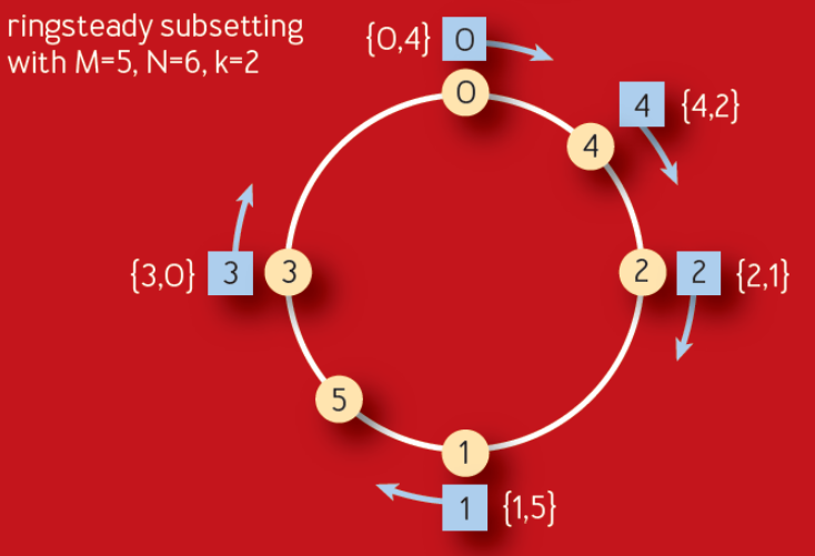
Subsetting was also top of mind after reading a recent ACM paper published by Google. It describes an improvement on their long-standing Deterministic Subsetting algorithm that they’ve used for many years. The Ringsteady algorithm (figure below) creates an evenly distributed ring of servers (yellow nodes) and then walks the ring to allocate them to each front-end task (blue nodes).
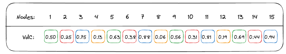
The algorithm relies on the idea of low-discrepancy numeric sequences to create a naturally balanced distribution ring that is more consistent than one built on a randomness-based consistent hash. The particular sequence used is a binary variant of the Van der Corput sequence. As long as the sequence of added servers is monotonically incrementing, for each additional server, the distribution will be evenly balanced between 0–1. Below is an example of what the binary Van der Corput sequence looks like.
Another big benefit of this distribution is that it provides a consistent expansion of the ring as servers are removed and added over time, evenly spreading new nodes among the subsets. This results in the stability of subsets and no cascading churn based on origin changes over time. Each node added or removed will only affect one subset, and new nodes will be added to a different subset every time.
Here’s a more concrete demonstration of the sequence above, in decimal form, with each number between 0–1 assigned to 4 subsets. In this example, each subset has 0.25 of that range depicted with its own color.
You can see that each new node added is balanced across subsets extremely well. If 50 nodes are added quickly, they will get distributed just as evenly. Similarly, if a large number of nodes are removed, it will affect all subsets equally.
The real killer feature, though, is that if a node is removed or added, it doesn’t require all the subsets to be shuffled and recomputed. Every single change will generally only create or remove one connection. This will hold for bigger changes, too, reducing almost all churn in the subsets.
Zuul’s Take
Our approach to implement this in Zuul was to integrate with Eureka service discovery changes and feed them into a distribution ring, based on the ideas discussed above. When new origins register in Zuul, we load their instances and create a new ring, and from then on, manage it with incremental deltas. We also take the additional step of shuffling the order of nodes before adding them to the ring. This helps prevent accidental hot spotting or overlap among Zuul instances.
The quirk in any load balancing algorithm from Google is that they do their load balancing centrally. Their centralized service creates subsets and load balances across their entire fleet, with a global view of the world. To use this algorithm, the key insight was to apply it to the event loops rather than the instances themselves. This allows us to continue having decentralized, client-side load balancing while also having the benefits of accurate subsetting. Although Zuul continues connecting to all origin servers, each event loop’s connection pool only gets a small subset of the whole. We end up with a singular, global view of the distribution that we can control on each instance — and a single sequence number that we can increment for each origin’s ring.
When a request comes in, Netty assigns it to an event loop, and it remains there for the duration of the request-response lifecycle. After running the inbound filters, we determine the destination and load the connection pool for this event loop. This will pull from a mapping of loop-to-subset, giving us the limited set of nodes we’re looking for. We then load balance using a modified choice-of-2, as discussed before. If this sounds familiar, it’s because there are no fundamental changes to how Zuul works. The only difference is that we provide a loop-bound subset of nodes to the load balancer as a starting point for its decision.
Another insight we had was that we needed to replicate the number of subsets among the event loops. This allows us to maintain low connection counts for large and small origins. At the same time, having a reasonable subset size ensures we can continue providing good balance and resiliency features for the origin. Most origins require this because they are not big enough to create enough instances in each subset.
However, we also don’t want to change this replication factor too often because it would cause a reshuffling of the entire ring and introduce a lot of churn. After a lot of iteration, we ended up implementing this by starting with an “ideal” subset size. We achieve this by computing the subset size that would achieve the ideal replication factor for a given cardinality of origin nodes. We can scale the replication factor across origins by growing our subsets until the desired subset size is achieved, especially as they scale up or down based on traffic patterns. Finally, we work backward to divide the ring into even slices based on the computed subset size.
Our ideal subset side is roughly 25–50 nodes, so an origin with 400 nodes will have 8 subsets of 50 nodes. On a 32-core instance, we’ll have a replication factor of 4. However, that also means that between 200 and 400 nodes, we’re not shuffling the subsets at all. An example of this subset recomputation is in the rollout graphs below.
An interesting challenge here was to satisfy the dual constraints of origin nodes with a range of cardinality, and the number of event loops that hold the subsets. Our goal is to scale the subsets as we run on instances with higher event loops, with a sub-linear increase in overall connections, and sufficient replication for availability guarantees. Scaling the replication factor elastically described above helped us achieve this successfully.
Subsetting Success
The results were outstanding. We saw improvements across all key metrics on Zuul, but most importantly, there was a significant reduction in total connection counts and churn.
Total Connections
This graph (as well as the ones below) shows a week’s worth of data, with the typical diurnal cycle of Netflix usage. Each of the 3 colors represents our deployment regions in AWS, and the blue vertical line shows when we turned on the feature.
Total connections at peak were significantly reduced in all 3 regions by a factor of 10x. This is a huge improvement, and it makes sense if you dig into how subsetting works. For example, a machine running 16 event loops could have 8 subsets — each subset is on 2 event loops. That means we’re dividing an origin by 8, hence an 8x improvement. As to why peak improvement goes up to 10x, it’s probably related to reduced churn (below).
Churn
This graph is a good proxy for churn. It shows how many TCP connections Zuul is opening per second. You can see the before and after very clearly. Looking at the peak-to-peak improvement, there is roughly an 8x improvement.
The decrease in churn is a testament to the stability of the subsets, even as origins scale up, down, and redeploy over time.
Looking specifically at connections created in the pool, the reduction is even more impressive:
The peak-to-peak reduction is massive and clearly shows how stable this distribution is. Although hard to see on the graph, the reduction went from thousands per second at peak down to about 60. Thereis effectively no churn of connections, even at peak traffic.
Load Balancing
The key constraint to subsetting is ensuring that the load balance on the backends is still consistent and evenly distributed. You’ll notice all the RPS on origin nodes grouped tightly, as expected. The thicker lines represent the subset size and the total origin size.
Balance at deployBalance 12 hours after deploy
In the second graph, you’ll note that we recompute the subset size (blue line) because the origin (purple line) became large enough that we could get away with less replication in the subsets. In this case, we went from a subset size of 100 for 400 servers (a division of 4) to 50 (a division of 8).
System Metrics
Given the significant reduction in connections, we saw reduced CPU utilization (~4%), heap usage (~15%), and latency (~3%) on Zuul, as well.
Zuul canary metrics
Rolling it Out
As we rolled this feature out to our largest origins — streaming playback APIs — we saw the pattern above continue, but with scale, it became more impressive. On some Zuul shards, we saw a reduction of as much as 13 million connections at peak, with almost no churn.
Today the feature is rolled out widely. We’re serving the same amount of traffic but with tens of millions fewer connections. Despite the reduction of connections, there is no decrease in resiliency or load balancing. H2 multiplexing allows us to scale up requests separately from connections, and our subsetting algorithm ensures an even traffic balance.
Although challenging to get right, subsetting is a worthwhile investment.
Acknowledgments
We would also like to thank Peter Ward, Paul Wankadia, and Kavita Guliani at Google for developing this algorithm and publishing their work for the benefit of the industry.
Anyone can take advantage of Cloudflare’s far-reaching network to protect and accelerate their online presence. Our vast number of data centers, and their proximity to Internet users around the world, enables us to secure and accelerate our customers’ Internet applications, APIs and websites. Even a simple service with a single origin server can leverage the massive scale of the Cloudflare network in 270+ cities. Using the Cloudflare cache, you can support more requests and users without purchasing new servers.
Whether it is to guarantee high availability through redundancy, or to support more dynamic content, an increasing number of services require multiple origin servers. The Cloudflare Load Balancer keeps our customer’s services highly available and makes it simple to spread out requests across multiple origin servers. Today, we’re excited to announce a frequently requested feature for our Load Balancer – Weighted Pools!
What’s a Weighted Pool?
Before we can answer that, let’s take a quick look at how our load balancer works and define a few terms:
Origin Servers – Servers which sit behind Cloudflare and are often located in a customer-owned datacenter or at a public cloud provider.
Origin Pool – A logical collection of origin servers. Most pools are named to represent data centers, or cloud providers like “us-east,” “las-vegas-bldg1,” or “phoenix-bldg2”. It is recommended to use pools to represent a collection of servers in the same physical location.
Traffic Steering Policy – A policy specifies how a load balancer should steer requests across origin pools. Depending on the steering policy, requests may be sent to the nearest pool as defined by latitude and longitude, the origin pool with the lowest latency, or based upon the location of the Cloudflare data center.
Pool Weight – A numerical value to describe what percentage of requests should be sent to a pool, relative to other pools.
When a request from a visitor arrives at the Cloudflare network for a hostname with a load balancer attached to it, the load balancer must decide where the request should be forwarded. Customers can configure this behavior with traffic steering policies.
The Cloudflare Load Balancer already supports Standard Steering, Geo Steering, Dynamic Steering, and Proximity Steering. Each of these respective traffic steering policies control how requests are distributed across origin pools. Weighted Pools are an extension of our standard, random steering policy which allows the specification of what relative percentage of requests should be sent to each respective pool.
In the example above, our load balancer has two origin pools, “las-vegas-bldg1” (which is a customer operated data center), and “us-east-cloud” (which is a public cloud provider with multiple virtual servers). Each pool has a weight of 0.5, so 50% of requests should be sent to each respective pool.
Why would someone assign weights to origin pools?
Before we built this, Weighted Pools was a frequently requested feature from our customers. Part of the reason we’re so excited about this feature is that it can be used to solve many types of problems.
Unequally Sized Origin Pools
In the example below, the amount of dynamic and uncacheable traffic has significantly increased due to a large sales promotion. Administrators notice that the load on their Las Vegas data center is too high, so they elect to dynamically increase the number of origins within their public cloud provider. Our two pools, “las-vegas-bldg1” and “us-east-cloud” are no longer equally sized. Our pool representing the public cloud provider is now much larger, so administrators change the pool weights so that the cloud pool receives 0.8 (80%) of the traffic, relative to the 0.2 (20%) of the traffic which the Las Vegas pool receives. The administrators were able to use pool weights to very quickly fine-tune the distribution of requests across unequally sized pools.
Data center kill switch
In addition to balancing out unequal sized pools, Weighted Pools may also be used to completely take a data center (an origin pool) out of rotation by setting the pool’s weight to 0. This feature can be particularly useful if a data center needs to be quickly eliminated during troubleshooting or a proactive maintenance where power may be unavailable. Even if a pool is disabled with a weight of 0, Cloudflare will still monitor the pool for health so that the administrators can assess when it is safe to return traffic.
Network A/B testing
One final use case we’re excited about is the ability to use weights to attract a very small amount of requests to pool. Did the team just stand up a brand-new data center, or perhaps upgrade all the servers to a new software version? Using weighted pools, the administrators can use a load balancer to effectively A/B test their network. Only send 0.05 (5%) of requests to a new pool to verify the origins are functioning properly before gradually increasing the load.
How do I get started?
When setting up a load balancer, you need to configure one or more origin pools, and then place origins into your respective pools. Once you have more than one pool, the relative weights of the respective pools will be used to distribute requests.
To set up a weighted pool using the Dashboard, create a load balancer in the Traffic > Load Balancing area.
Once you have set up the load balancer, you’re navigated to the Origin Pools setup page. Under the Traffic Steering Policy, select Random, and then assign relative weights to every pool.
If your weights do not add up to 1.00 (100%), that’s fine! We will do the math behind the scenes to ensure how much traffic the pool should receive relative to other pools.
Weighted Pools may also be configured via the API. We’ve edited an example illustrating the relevant parts of the REST API.
The load balancer should employ a “steering_policy” of random.
Each pool has a UUID, which can then be assigned a “pool_weight.”
We’re excited to launch this simple, yet powerful and capable feature. Weighted pools may be utilized in tons of creative new ways to solve load balancing challenges. It’s available for all customers with load balancers today!
Today, we are announcing the general availability of Cloudflare Waiting Room to customers on our Enterprise plans, making it easier than ever to protect your website against traffic spikes. We are also excited to present several new features that have user experience in mind — an alternative queueing method and support for custom web/mobile applications.
First-In-First-Out (FIFO) Queueing
Whether you’ve waited to check out at a supermarket or stood in line at a bank, you’ve undoubtedly experienced FIFO queueing. FIFO stands for First-In-First-Out, which simply means that people are seen in the order they arrive — i.e., those who arrive first are processed before those who arrive later.
When Waiting Room was introduced earlier this year, it was first deployed to protect COVID-19 vaccine distributors from overwhelming demand — a service we offer free of charge under Project Fair Shot. At the time, FIFO queueing was the natural option due to its wide acceptance in day-to-day life and accurate estimated wait times. One problem with FIFO is that users who arrive later could see long estimated wait times and decide to abandon the website.
We take customer feedback seriously and improve products based on it. A frequent request was to handle users irrespective of the time they arrive in the Waiting Room. In response, we developed an additional approach: random queueing.
A New Approach to Fairness: Random Queueing
You can think of random queueing as participating in a raffle for a prize. In a raffle, people obtain tickets and put them into a big container. Later, tickets are drawn at random to determine the winners. The more time you spend in the raffle, the better your chances of winning at least once, since there will be fewer tickets in the container. No matter what, everyone participating in the raffle has an opportunity to win.
Similarly, in a random queue, users are selected from the Waiting Room at random, regardless of their initial arrival time. This means that you could be let into the application before someone who arrived earlier than you, or vice versa. Just like how you can buy more tickets in a raffle, joining a random queue earlier than someone else will give you more attempts to be accepted, but does not guarantee you will be let in. However, at any particular time, you will have the same chance to be let into the website as anyone else. This is different from a raffle, where you could have more tickets than someone else at a given time, providing you with an advantage.
Random queueing is designed to give everyone a fair chance. Imagine waking up excited to purchase new limited-edition sneakers only to find that the FIFO queue is five hours long and full of users that either woke up in the middle of the night to get in line or joined from earlier time zones. Even if you waited five hours, those sneakers would likely be sold out by the time you reach the website. In this case, you’d probably abandon the Waiting Room completely and do something else. On the other hand, if you were aware that the queue was random, you’d likely stick around. After all, you have a chance to be accepted and make a purchase!
As a result, random queueing is perfect for short-lived scenarios with lots of hype, such as product launches, holiday traffic, special events, and limited-time sales.
By contrast, when the event ends and traffic returns to normal, a FIFO queue is likely more suitable, since its widely accepted structure and accurate estimated wait times provide a consistent user experience.
How Does Random Queueing Work?
Perhaps the best part about random queueing is that it maintains the same internal structure that powers FIFO. As a result, if you change the queueing method in the dashboard — even when you may be actively queueing users — the transition to the new method is seamless. Imagine you have users 1, 2, 3, 4, and 5 waiting in a FIFO queue in the order 5 → 4 → 3 → 2 → 1, where user 1 will be the next user to access the application. Let’s assume you switch to random queueing. Now, any user can be accepted next. Let’s assume user 4 is accepted. If you decide to immediately switch back to FIFO queueing, the queue will reflect the order 5 → 3 → 2 → 1. In other words, transitioning from FIFO to random and back to FIFO will respect the initial queue positions of the users! But how does this work? To understand, we first need to remember how we built Waiting Room for FIFO.
Recall the Waiting Room configurations:
Total Active Users. The total number of active users that can be using the application at any given time.
New Users Per Minute.The maximum number of new users per minute that can be accepted to the application.
Next, remember that Waiting Room is powered by cookies. When you join the Waiting Room for the first time, you are assigned an encrypted cookie. You bring this cookie back to the Waiting Room and update it with every request, using it to prove your initial arrival time and status.
Properties in the Waiting Room cookie include:
bucketId. The timestamp rounded down to the nearest minute of the user’s first request to the Waiting Room. If you arrive at 10:23:45, you will be grouped into a bucket for 10:23:00.
acceptedAt. The timestamp when the user got accepted to the origin website for the first time.
refreshIntervalSeconds. When queueing, this is the number of seconds the user must wait before sending another request to the Waiting Room.
lastCheckInTime. The last time each user checked into the Waiting Room or origin website. When queueing, this is only updated for requests every refreshIntervalSeconds.
For any given minute, we can calculate the number of users we can let into the origin website. Let’s say we deploy a Waiting Room on “https://example.com/waitingroom” that can support 10,000 Total Active Users, and we allow up to 2,000 New Users Per Minute. If there are currently 7,000 active users on the website, we have 10,000 – 7,000 = 3,000 open slots. However, we need to take the minimum (3,000, 2,000) = 2,000 since we need to respect the New Users Per Minute limit. Thus, we have 2,000 available slots we can give out.
Let’s assume there are 2,500 queued users that joined over the last three minutes in groups of 500, 1,000, and 1,000, respectively for the timestamps 15:54, 15:55, and 15:56. To respect FIFO queueing, we will take our 2,000 available slots and try to reserve them for users who joined first. Thus, we will reserve 500 available slots for the users who joined at 15:54 and then reserve 1000 available slots for the users who joined at 15:55. When we get to the users for 15:56, we see that we only have 500 slots left, which is not enough for the 1,000 queued users for this minute:
Since we have reserved slots for all users with bucketIds of 15:54 and 15:55, they can be let into the origin website from any data center. However, we can only let in a subset of the users who initially arrived at 15:56.
Timestamp (bucketId)
Queued Users
Reserved Slots
Strategy
15:54
500
500
Accept all users
15:55
1,000
1,000
Accept all users
15:56
1,000
500
Accept subset of users
These 500 slots for 15:56 are allocated to each Cloudflare edge data center based on its respective historical traffic data, and further divided for each Cloudflare Worker within the data center. For example, let’s assume there are two data centers — Nairobi and Dublin — which share 60% and 40% of the traffic, respectively, for this minute. In this case, we will allocate 500 * .6 = 300 slots for Nairobi and 500 * .4 = 200 slots for Dublin. In Nairobi, let’s say there are 3 active workers, so we will grant each of them 300 / 3 = 100 slots. If you make a request to a worker in Nairobi and your bucketId is 15:56, you will be allowed in and consume a slot if the worker still has at least one of its 100 slots available. Since we have reserved all 2,000 available slots, users with bucketIds after 15:56 will have to continue queueing.
Let’s modify this case and assume we only have 200 queued users, all of which are in the 15:54 bucket. First, we reserve 200 slots for these queued users, leaving us 2,000 – 200 = 1,800 remaining slots. Since we have reserved slots for all queued users, we can use the remaining 1,800 slots on new users — people who have just made their first request to the Waiting Room and don’t have a cookie or bucketId yet. Similar to how we handle buckets with fewer slots than queued users, we will distribute these 1,800 slots to each data center, allocating 1,800 * .6 = 1,080 to Nairobi and 1,800 * .4 = 720 to Dublin. In Nairobi, we will split these equally across the 3 workers, giving them 1,080 / 3 = 360 slots each. If you are a new user making a request to a worker in Nairobi, you will be accepted and take a slot if the worker has at least one of its 360 slots available, otherwise you will be marked as a queued user and enter the Waiting Room.
Now that we have outlined the concepts for FIFO, we can understand how random queueing operates. Simply put, random queueing functions the same way as FIFO, except we pretend that every user is new. In other words, we will not look at reserved slots when making the decision if the user should be let in. Let’s revisit the last case with 200 queued users in the 15:54 bucket and 2,000 available slots. When random queueing, we allocate the full 2,000 slots to new users, meaning Nairobi gets 2,000 * .6 = 1,200 slots and each of its 3 workers gets 1,200 / 3 = 400 slots. No matter how many users are queued or freshly joining the Waiting Room, all of them will have a chance at taking these slots.
Finally, let’s reiterate that we are only pretending that all users are new — we still assign them to bucketIds and reserve slots as if we were FIFO queueing, but simply don’t make any use of this logic while random queueing is active. That way, we can maintain the same FIFO structure while we are random queueing so that if necessary, we can smoothly transition back to FIFO queueing and respect initial user arrival times.
How “Random” is Random Queueing?
Since random queueing is basically a race for available slots, we were concerned that it could be exploited if the available user slots and the queued user check-ins did not occur randomly.
To ensure all queued users can attempt to get into the website at the same rate, we store (in the encrypted cookie) the last time each user checked into the Waiting Room (lastCheckInTime) to prevent them from attempting to gain access to the website until a number of seconds have passed (refreshIntervalSeconds). This means that spamming the page refresh button will not give you an advantage over other queued users! Be patient — the browser will refresh automatically the moment you are eligible for another chance.
Next, let’s imagine five queued users checking into the Waiting Room every refreshIntervalSeconds=30 at approximately the :00 and :30 minute marks. A new queued user joins the Waiting Room and checks in at approximately :15 and :45. If new slots are randomly released, this new user will have about a 50% chance of being selected next, since it monopolizes over the :00-15 and :30-45 ranges. On the other hand, the other five queued users share the :15-30 and :45-00 ranges, giving them about a 50% / 5 = 10% chance each. Let’s consider that new slots are not randomly released and assume they are always released at :59. In this case, the new queued user will have virtually no chance to be selected before the other five queued users because these users will always check in one second later at :00, immediately consuming any newly released slots.
To address this vulnerability, we changed our implementation to ensure that slots are released randomly and encouraged users to check in at random offsets from each other. To help split up users that are checking in at similar times, we vary each user’s refreshIntervalSeconds by a small, pseudo-randomly generated offset for each check-in and store this new refresh interval in the encrypted Waiting Room cookie for validation on the next request. Thus, a user who previously checked in every 30 seconds might now check in after 29 seconds, then 31 seconds, then 27 seconds, and so on — but still averaging a 30-second refresh interval. Over time, these slight check-in variations become significant, spreading out user check-in times and strengthening the randomness of the queue. If you are curious to learn more about the apparent “randomness” behind mixing user check-in intervals, you can think of it as a chaotic system subjected to the butterfly effect.
Nevertheless, we weren’t convinced our efforts were enough and wanted to test random queueing empirically to validate its integrity. We conducted a simulation of 10,000 users joining a Waiting Room uniformly across 30 minutes. When let into the application, users spent approximately 1 minute “browsing” before they stopped checking in. We ran this experiment for both FIFO and random queueing and graphed each user’s observed wait time in seconds in the Waiting Room against the minute they initially arrived (starting from 0). Recall that users are grouped by minute using bucketIds, so each user’s arrival minute is truncated down to the current minute.
Based on our data, we can see immediately for FIFO queueing that, as the arrival minute increases, the observed wait time increases linearly. This makes sense for a FIFO queue, since the “line” will just get longer if there are more users entering the queue than leaving it. For each arrival minute, there is very little variation among user wait times, meaning that if you and your friend join a Waiting Room at approximately the same time, you will both be accepted around the same time. If you join a couple of minutes before your friend, you will almost always be accepted first.
When looking at the results for random queueing, we observe users experiencing varied wait times regardless of the arrival minute. This is expected, and helps prove the “randomness” of the random queue! We can see that, if you join five minutes after your friend, although your friend will have more chances to get in, you may still be accepted first! However, there are so many data points overlapping with each other in the plot that it is hard to tell how they are distributed. For instance, it could be possible that most of these data points experience extreme wait times, but as humans we aren’t able to tell.
import json
import numpy as np
import matplotlib.pyplot as plt
import sys

filename = sys.argv[1]

with open(filename) as file:
   data = json.load(file)

   x = data["ArrivalMinutes"]
   y = data["WaitTimeSeconds"]

   heatmap, _, _ = np.histogram2d(x, y, bins=(30, 30))

   plt.clf()
   plt.title(filename)
   plt.xlabel('Arrival Minute Buckets')
   plt.ylabel('WaitTime Buckets')
   plt.imshow(heatmap.T, origin='lower')
   plt.show()
The heatmaps display where the data points are concentrated in the original plot, using brighter (hotter) colors to represent areas containing more points:
By inspecting the generated heatmaps, we can conclude that FIFO and random queueing are working properly. For FIFO queueing, users are being accepted in the order they arrive. For random queueing, we can see that users are accepted to the origin regardless of arrival time. Overall, we can see the heatmap for random queueing is well distributed, indicating it is sufficiently random!
If you are curious why random queueing has very hot colors along the lowest wait times followed by very dark colors afterward, it is actually because of how we are simulating the queue. For the simulation, we spoofed the bucketIds of the users and let them all join the Waiting Room at once to see who would be let in first. In the random queueing heatmap, the bright colors along the lowest wait time buckets indicate that many users were accepted quickly after joining the queue across all bucketIds. This is expected, demonstrating that random queueing does not give an edge to users who join earlier, giving each user a fair chance regardless of its bucketId. The reason why these users were almost immediately accepted in WaitTime Bucket 0 is because this simulation started with no users on the origin, meaning new users would be accepted until the Waiting Room limits were reached. Since this first wave of accepted users “browsed” on the origin for a minute before leaving, no additional users during this time were let in. Thus, the colors are very dark for WaitTime Buckets 1 and 2. Similarly, the second wave of users is randomly selected afterward, followed by another period of time when no users were accepted in WaitTime Bucket 5. As the wait time increases, the more attempts a particular user will have to be let in, meaning it is unlikely for users to have extreme wait times. We can see this by observing the colors grow darker as the WaitTime Bucket approaches 29.
How Is Estimated Time Calculated for Random Queueing?
In a random queue, you can be accepted at any moment… so how can you display an estimated wait time? For a particular user, this is an impossible task, but when you observe all the users together, you can accurately account for most user experiences using a probabilistic estimated wait time range.
At any given moment, we know:
letInPerMinute. The current average users per minute being let into the origin.
currentlyWaiting. The current number of users waiting in the queue.
Therefore, we can calculate the probability of a user being let into the origin in the next minute:
If there are 100 users waiting in the queue, and we are currently letting in 10 users per minute, the probability a user will be let in over the next minute is 10 / 100 = .1 (10%).
Using P(LetInOverMinute), we can determine the n minutes needed for a p chance of being let into the origin:
p = 1 – (1 – P(LetInOverMinute))n
Recall that the probability of getting in at least once is the complement of not getting in at all. The probability of not being let into the origin over n minutes is (1 – P(LetInOverMinutes))n. Therefore, the probability of getting in at least once is 1 – (1 – P(LetInOverMinute))n. This equation can be simplified further:
n = log(1 – p) / log(1 – P(LetInOverMinute))
Thus, if we want to calculate the estimated wait time to have a p = .5 (50%) chance of getting into the origin with the probability of getting let in during a particular minute P(LetInOverMinute) = .1 (10%), we calculate:
n = log(1 – .5) / log(1 – .1) ≈ 6.58 minutes or 6 minutes and 35 seconds
In this case, we estimate that 50% of users will wait less than 6 minutes and 35 seconds and the remaining 50% of users will wait longer than this.
So, which estimated wait times are displayed to the user? It is up to you! If you create a Mustache HTML template for a Waiting Room, you will now be able to use the variables waitTime25Percentile, waitTime50Percentile, and waitTime75Percentile to display the estimated wait times in minutes when p = .25, p = .5, and p = .75, respectively. There are also new variables that are used to display and determine the queueing method, such as queueingMethod, isFIFOQueue, and isRandomQueue. If you want to display something more dynamic like a custom view in a mobile app, keep reading to learn about our new JSON response, which provides a REST API for the same set of variables.
Supporting Dynamic Applications with a JSON Response
Before, customers could only deploy static Mustache HTML templates to customize the style of their Waiting Rooms. These templates work well for most use cases, but fall short if you want to display anything that requires state. Let’s imagine you’re queueing to buy concert tickets on your mobile device, and you see an embedded video of your favorite song. Naturally, you click on it and start singing along! A couple seconds later, the browser refreshes the page automatically to update your status in the Waiting Room, resetting your video to the start.
The purpose of the new JSON response is to give full control to a custom application, allowing it to determine what to display to the user and when to refresh. As a result, the application can maintain state and make sure your videos are never interrupted again!
Once the JSON response is enabled for a Waiting Room, any request to the Waiting Room with the header Accept: application/json will receive a JSON object with all the fields from the Mustache template.
An example request when the queueing method is FIFO:
Don’t forget that Waiting Room uses a cookie to maintain a user’s status! Without a cookie in the request, the Waiting Room will think the user has just joined the queue.
Don’t forget to refresh! Inspect the ‘Refresh’ HTTP response header or the refreshIntervalSeconds property and send another request to the Waiting Room after that number of seconds.
Keep in mind that if the user’s request is let into the origin, JSON may not necessarily be returned. To gracefully parse all responses, send JSON from the origin website if the header Accept: application/json is present. For example, the origin could return:
SameSite and Secure are attributes in the HTTP response Set-Cookie header. SameSite is used to determine when cookies are sent to a website while Secure indicates if there must be a secure context (HTTPS).
There are three different values of SameSite:
SameSite=Lax.This is the default value when the SameSite attribute is not present. Cookies are not sent on cross-site sub-requests unless the user is following a link to the third-party site. If you are on example1.com, cookies will not be sent to example2.com unless you click a link that navigates to example2.com.
SameSite=Strict. Cookies are sent only in first-party contexts. If you are on example1.com, cookies will never be sent to example2.com even if you click a link that navigates to example2.com.
SameSite=None. Cookies are sent for all contexts, but the Secure attribute must be set. If you are on example1.com, cookies will be sent to example2.com for all sub-requests. If Secure is not set, the browser will block the cookie.
IFrames (Inline Frames) allow HTML documents to embed other HTML documents, such as an advertisement, video, or webpage. When an application from a third-party website is rendered inside an IFrame, cookies will only be sent to it if SameSite=None is set.
Why is this all important? In the past, we did not set SameSite, meaning it defaulted to SameSite=Lax for all responses. As a result, a user queueing through an IFrame would never have its cookie updated and appear to the Waiting Room as joining for the first time on every request. Today, we are introducing customization for both the SameSite and Secure attributes, which will allow Waiting Rooms to be displayed in IFrames!
At the moment, this is only configurable through the Cloudflare API. By default, the configuration for SameSite and Secure will be set to “auto”, automatically selecting the most flexible option. In this case, SameSite will be set to None if Always Use HTTPS is enabled, otherwise it will be set to Lax. Similarly, Secure will only be set if Always Use HTTPS is enabled. In other words, Waiting Room IFrames will work properly by default as long as Always Use HTTPS is toggled. If you are wondering why Always Use HTTPS is used here, remember that SameSite=None requires that Secure is also set, or else the browser will block the Waiting Room cookie.
If you decide to manually configure the behavior of SameSite and Secure through the API, be careful! We do guard against setting SameSite=None without Secure, but if you decide to set Secure on every request (secure=”always”) and don’t have Always Use HTTPS enabled, this means that a user who sends an insecure (HTTP) request to the Waiting Room will have its cookie blocked by its browser!
If you want to explore using IFrames with Waiting Room yourself, here is a simple example of a Cloudflare Worker that renders the Waiting Room on “https://example.com/waitingroom” in an IFrame:
Waiting Room still has plenty of room to grow! Every day, we are seeing more Waiting Rooms deployed to protect websites from traffic spikes. As Waiting Room continues to be used for new purposes, we will keep adding features to make it as customizable and user-friendly as possible.
Stay tuned — what we have announced today is just the tip of the iceberg of what we have planned for Waiting Room!
Load Balancing — functionality that’s been around for the last 30 years to help businesses leverage their existing infrastructure resources. Load balancing works by proactively steering traffic away from unhealthy origin servers and — for more advanced solutions — intelligently distributing traffic load based on different steering algorithms. This process ensures that errors aren’t served to end users and empowers businesses to tightly couple overall business objectives to their traffic behavior.
What’s important for load balancing today?
We are no longer in the age where setting up a fixed amount of servers in a data center is enough to meet the massive growth of users browsing the Internet. This means that we are well past the time when there is a one size fits all solution to suffice the needs of different businesses. Today, customers look for load balancers that are easy to use, propagate changes quickly, and — especially now — provide the most feature flexibility. Feature flexibility has become so important because different businesses have different paths to success and, consequently, different challenges! Let’s go through a few common use cases:
You might have an application split into microservices, where specific origins support segments of your application. You need to route your traffic based on specific paths to ensure no single origin can be overwhelmed and users get sent to the correct server to answer the originating request.
You may want to route traffic based on a specific value within a header request such as “PS5” and send requests to the data center with the matching header.
If you heavily prioritize security and privacy, you may adopt a split-horizon DNS setup within your network architecture. You might choose this architecture to separate internal network requests from public requests from the rest of the public Internet. Then, you could route each type of request to pools specifically suited to handle the amount and type of traffic.
As we continue to build new features and products, we also wanted to build a framework that would allow us to increase our velocity to add new items to our Load Balancing solution while we also take the time to create first class features as well. The result was the creation of our custom rule builder!
Now you can build complex, custom rules to direct traffic using Cloudflare Load Balancing, empowering customers to create their own custom logic around their traffic steering and origin selection decisions. As we mentioned, there is no one size fits all solution in today’s world. We provide the tools to easily and quickly create rules that meet the exact requirements needed for any customer’s unique situation and architecture. On top of that, we also support ‘and’ and ‘or’ statements within a rule, allowing very powerful and complex rules to be created for any situation!
Load Balancing by path becomes easy, requiring just a few minutes to enter the paths and some boolean statements to create complex rules. Steer by a specific header, query string, or cookie. It’s no longer a pain point. Leverage a split horizon DNS design by creating a rule looking at the IP source address and then routing to the appropriate pool based on the value. This is just a small subset of the very robust capabilities that load balancing custom rules makes available to our users and this is just the start! Not only do we have a large amount of functionality right out of the box, but we’re also providing a consistent, intuitive experience by building on our Firewall Rules Engine.
Let’s go through some use cases to explore how custom rules can open new possibilities by giving you more granular control of your traffic.
High-volume transactions for ecommerce
For any high-volume transaction business such as an ecommerce or retail store, ensuring the transactions go through as fast and reliably as possible is a table stakes requirement. As transaction volume increases, no single origin can handle the incoming traffic, and it doesn’t always make sense for it to do so. Why have a transaction request travel around the world to a specifically nominated origin for payment processing? This setup would only add latency, leading to degraded performance, increased errors, and a poor customer experience. But what if you could create custom logic to segment transactions to different origin servers based on a specific value in a query string, such as a PS5 (associated with Sony’s popular PlayStation 5)? What if you could then couple that value with dynamic latency steering to ensure your load balancer always chooses the most performant path to the origin? This would be game changing to not only ensure that table-stakes transactions are reliable and fast but also drastically improve the customer experience. You could do this in minutes with load balancing custom rules:
For any requests where the query string shows ‘PS5’, then route based on which pool is the most performant.
Load balance across multiple DNS vendors to support privacy and security
Some customers may want to use multiple DNS providers to bolster their resiliency along with their security and privacy for the different types of traffic going through their network. By utilizing two DNS providers, customers can not only be sure that they remain highly available in times of outages, but also direct different types of traffic, whether that be internal network traffic across offices or unknown traffic from the public Internet.
Without flexibility, however, it can be difficult to easily and intelligently route traffic to the proper data centers to maintain that security and privacy posture. Not anymore! With load balancing custom rules, supporting a split horizon DNS architecture takes as little as five minutes to set up a rule based on the IP source condition and then overwriting which pools or data centers that traffic should route to.
This can also be extremely helpful if your data centers are spread across multiple areas of the globe that don’t align with the 13 current regions within Cloudflare. By segmenting where traffic goes based on the IP source address, you can create a type of geo-steering setup that is also finely tuned to the requirements of the business!
How did we build it?
We built Load Balancing rules on top of our open-source wirefilter execution engine. People familiar with Firewall Rules and other products will notice similar syntax since both products are built on top of this execution engine.
By reusing the same underlying engine, we can take advantage of a battle-tested production library used by other products that have the performance and stability requirements of their own. For those experienced with our rule-based products, you can reuse your knowledge due to the shared syntax to define conditionals statements. For new users, the Wireshark-like syntax is often familiar and relatively simple.
DNS vs Proxied?
Our Load Balancer supports both DNS and Proxied load balancing. These two protocols operate very differently and as such are handled differently.
For DNS-based load balancing, our load balancer responses to DNS queries sent from recursive resolvers. These resolvers are normally not the end user directly requesting the traffic nor is there a 1-to-1 ratio between DNS query and end-user requests. The DNS makes extensive use of caching at all levels so the result of each query could potentially be used by thousands of users. Combined, this greatly limits the possible feature set for DNS. Since you don’t see the end user directly nor know if your response is going to be used by one or more users, all responses can only be customized to a limited degree.
Our Proxied load balancing, on the other hand, processes rules logic for every request going through the system. Since we act as a proxy for all these requests, we can invoke this logic for all requests and access user-specific data.
These different modes mean the fields available to each end up being quite different. The DNS load balancer gets access to DNS-specific fields such as “dns.qry.name” (the query name) while our Proxied load balancer has access to “http.request.method” (the HTTP method used to access the proxied resource). Some more general fields — like the name of the load balancer being used — are available in both modes.
How does it work under the hood?
When a load balancer rule is configured, that API call will validate that the conditions and actions of the rules are valid. It makes sure the condition only references known fields, isn’t excessively long, and is syntactically valid. The overrides are processed and applied to the load balancers configuration to make sure they won’t cause an invalid configuration. After validation, the new rule is saved to our database.
With the new rule saved, we take the load balancer’s data and all rules used by it and package that data together into one configuration to be shipped out to our edge. This process happens very quickly, so any changes are visible to you in just a few seconds.
While DNS and proxied load balancers have access to different fields and the protocols themselves are quite different, the two code paths overlap quite a bit. When either request type makes it to our load balancer, we first load up the load balancer specific configuration data from our edge datastore. This object contains all the “static” data for a load balancer, such as rules, origins, pools, steering policy, and so forth. We load dynamic data such as origin health and RTT data when evaluating each pool.
At the start of the load balancer processing, we run our rules. This ends up looking very much like a loop where we check each condition and — if the condition is true — we apply the effects specified by the rules. After each condition is processed and the effects are applied we then run our normal load balancing logic as if you have configured the load balancer with the overridden settings. This style of applying each override in turn allows more than one rule to change a given setting multiple times during execution. This lets users avoid extremely long and specific conditionals and instead use shorter conditionals and rule ordering to override specific settings creating a more modular ruleset.
What’s coming next?
For you, the next steps are simple. Start building custom load balancing rules! For more guidance, check out our developer documentation.
For us, we’re looking to expand this functionality. As this new feature develops, we are going to be identifying new fields for conditionals and new options for overrides to allow more specific behavior. As an example, we’ve been looking into exposing a means to creating more time-based conditionals, so users can create rules that only apply during certain times of the day or month. Stay tuned to the blog for more!
Today, we are excited to announce Cloudflare Waiting Room! It will first be available to select customers through a new program called Project Fair Shot which aims to help with the problem of overwhelming demand for COVID-19 vaccinations causing appointment registration websites to fail. General availability in our Business and Enterprise plans will be added in the near future.
Wait, you’re excited about a… Waiting Room?
Most of us are familiar with the concept of a waiting room, and rarely are we excited about the idea of being in one. Usually our first experience of one is at a doctor’s office — yes, you have an appointment, but sometimes the doctor is running late (or one of the patients was). Given the doctor can only see one person at a time… the waiting room was born, as a mechanism to queue up patients.
While servers can handle more concurrent requests than a doctor can, they too can be overwhelmed. If, in a pre-COVID world, you’ve ever tried buying tickets to a popular concert or event, you’ve probably encountered a waiting room online. It limits requests inbound to an application, and places these requests into a virtual queue. Once the number of users in the application has reduced, new users are let in within the defined thresholds the application can handle. This protects the origin servers supporting the application from being inundated with too many requests, while also ensuring equity from a user perspective — users who try to access a resource when the system is overloaded are not unfairly dropped and forced to reconnect, hoping to join their chance in the queue.
Why Now?
Given not many of us are going to live concerts any time soon, why is Cloudflare doing this now?
Well, perhaps we aren’t going to concerts, but the second order effects of COVID-19 have created a huge need for waiting rooms. First of all, given social distancing and the closing of many places of business and government, customers and citizens have shifted to online channels, putting substantially more strain on business and government infrastructure.
Second, the pandemic and the flow-on consequences of it have meant many folks around the world have come to rely on resources that they didn’t need twelve months earlier. To be specific, these are often health or government-related resources — for example, unemployment insurance websites. The online infrastructure was set up to handle a peak load that didn’t foresee the impact of COVID-19. We’re seeing a similar pattern emerge with websites that are related to vaccines.
Historically, the number of organizations that needed waiting rooms was quite small. The nature of most businesses online usually involve a more consistent user load, rather than huge crushes of people all at once. Those organizations were able to build custom waiting rooms and were integrated deeply into their application (for example, buying tickets). With Cloudflare’s Waiting Room, no code changes to the application are necessary and a Waiting Room can be set up in a matter of minutes for any website without writing a single line of code.
Whether you are an engineering architect or a business operations analyst, setting up a Waiting Room is simple. We make it quick and easy to ensure your applications are reliable and protected from unexpected spikes in traffic. Other features we felt were important are automatic enablement and dynamic outflow. In other words, a waiting room should turn on automatically when thresholds are exceeded and as users finish their tasks in the application, let out different sized buckets of users and intake new ones already in the queue. It should just work. Lastly, we’ve seen the major impact COVID-19 has made on users and businesses alike, especially, but not limited to, the health and government sectors. We wanted to provide another way to ensure these applications remain available and functional so all users can receive the care that they need and not errors within their browser.
How does Cloudflare’s Waiting Room work?
We built Waiting Room on top of our edge network and our Workers product. By leveraging Workers and our new Durable Objects offerings, we were able to remove the need for any customer coding and provide a seamless, out of the box product that will ‘just work’. On top of this, we get the benefits of the scale and performance of our Workers product to ensure we maintain extremely low latency overhead, keep estimated times presented to end users accurate as can be and not keep any user in the queue longer than needed. But building a centralized system in a decentralized network is no easy task. When requests come into an application from around the world, we need to be able to get a broad, accurate view of what that load looks like inbound and outbound to a given application.
Request going through Cloudflare without a Waiting Room
These requests, as fast as they are, still take time to travel across the planet. And so, a unique edge case was presented. What if a website is getting reasonable traffic from North America and Europe, but then a sudden major spike of traffic takes place from South America – how do we know when to keep letting users into the application and when to kick in the Waiting Room to protect the origin servers from being overloaded?
Thanks to some clever engineering and our Workers product, we were able to create a system that almost immediately keeps itself synced with global demand to an application giving us the necessary insight into when we should and should not be queueing users into the Waiting Room. By leveraging our global Anycast network and over 200+ data centers, we remove any single point of failure to protect our customers’ infrastructure yet also provide a great experience to end-users who have to wait a small amount of time to enter the application under high load.
Request going through Cloudflare with a Waiting Room
How to setup a Waiting Room
Setting up a Waiting Room is incredibly easy and very fast! At the easiest side of the scale, a user needs to fill out only five fields: 1) the name of the Waiting Room, 2) a hostname (which will already be pre-populated with the zone it’s being configured on), 3) the total active users that can be in the application at any given time, 4) the new users per minute allowed into the application, and 5) the session duration for any given user. No coding or any application changes are necessary.
We provide the option of using our default Waiting Room template for customers who don’t want to add additional branding. This simplifies the process of getting a Waiting Room up and running.
That’s it! Press save and the Waiting Room is ready to go!
For customers with more time and technical ability, the same process is followed, except we give full customization capabilities to our users so they can brand the Waiting Room, ensuring it matches the look and feel of their overall product.
Lastly, managing different Waiting Rooms is incredibly easy. With our Manage Waiting Room table, at a glance you are able to get a full snapshot of which rooms are actively queueing, not queueing, and/or disabled.
We are very excited to put the power of our Waiting Room into the hands of our customers to ensure they continue to focus on their businesses and customers. Keep an eye out for another blog post coming soon with major updates to our Waiting Room product for Enterprise!
As the scale of Cloudflare’s edge network has grown, we sometimes reach the limits of parts of our architecture. About two years ago we realized that our existing solution for spreading load within our data centers could no longer meet our needs. We embarked on a project to deploy a Layer 4 Load Balancer, internally called Unimog, to improve the reliability and operational efficiency of our edge network. Unimog has now been deployed in production for over a year.
This post explains the problems Unimog solves and how it works. Unimog builds on techniques used in other Layer 4 Load Balancers, but there are many details of its implementation that are tailored to the needs of our edge network.
The role of Unimog in our edge network
Cloudflare operates an anycast network, meaning that our data centers in 200+ cities around the world serve the same IP addresses. For example, our own cloudflare.com website uses Cloudflare services, and one of its IP addresses is 104.17.175.85. All of our data centers will accept connections to that address and respond to HTTP requests. By the magic of Internet routing, when you visit cloudflare.com and your browser connects to 104.17.175.85, your connection will usually go to the closest (and therefore fastest) data center.
Inside those data centers are many servers. The number of servers in each varies greatly (the biggest data centers have a hundred times more servers than the smallest ones). The servers run the application services that implement our products (our caching, DNS, WAF, DDoS mitigation, Spectrum, WARP, etc). Within a single data center, any of the servers can handle a connection for any of our services on any of our anycast IP addresses. This uniformity keeps things simple and avoids bottlenecks.
But if any server within a data center can handle any connection, when a connection arrives from a browser or some other client, what controls which server it goes to? That’s the job of Unimog.
There are two main reasons why we need this control. The first is that we regularly move servers in and out of operation, and servers should only receive connections when they are in operation. For example, we sometimes remove a server from operation in order to perform maintenance on it. And sometimes servers are automatically removed from operation because health checks indicate that they are not functioning correctly.
The second reason concerns the management of the load on the servers (by load we mean the amount of computing work each one needs to do). If the load on a server exceeds the capacity of its hardware resources, then the quality of service to users will suffer. The performance experienced by users degrades as a server approaches saturation, and if a server becomes sufficiently overloaded, users may see errors. We also want to prevent servers being underloaded, which would reduce the value we get from our investment in hardware. So Unimog ensures that the load is spread across the servers in a data center. This general idea is called load balancing (balancing because the work has to be done somewhere, and so for the load on one server to go down, the load on some other server must go up).
Note that in this post, we’ll discuss how Cloudflare balances the load on its own servers in edge data centers. But load balancing is a requirement that occurs in many places in distributed computing systems. Cloudflare also has a Layer 7 Load Balancing product to allow our customers to balance load across their servers. And Cloudflare uses load balancing in other places internally.
Deploying Unimog led to a big improvement in our ability to balance the load on our servers in our edge data centers. Here’s a chart for one data center, showing the difference due to Unimog. Each line shows the processor utilization of an individual server (the colour of the lines indicates server model). The load on the servers varies during the day with the activity of users close to this data center.The white line marks the point when we enabled Unimog. You can see that after that point, the load on the servers became much more uniform. We saw similar results when we deployed Unimog to our other data centers.
How Unimog compares to other load balancers
There are a variety of techniques for load balancing. Unimog belongs to a category called Layer 4 Load Balancers (L4LBs). L4LBs direct packets on the network by inspecting information up to layer 4 of the OSI network model, which distinguishes them from the more common Layer 7 Load Balancers.
The advantage of L4LBs is their efficiency. They direct packets without processing the payload of those packets, so they avoid the overheads associated with higher level protocols. For any load balancer, it’s important that the resources consumed by the load balancer are low compared to the resources devoted to useful work. At Cloudflare, we already pay close attention to the efficient implementation of our services, and that sets a high bar for the load balancer that we put in front of those services.
The downside of L4LBs is that they can only control which connections go to which servers. They cannot modify the data going over the connection, which prevents them from participating in higher-level protocols like TLS, HTTP, etc. (in contrast, Layer 7 Load Balancers act as proxies, so they can modify data on the connection and participate in those higher-level protocols).
L4LBs are not new. They are mostly used at companies which have scaling needs that would be hard to meet with L7LBs alone. Google has published about Maglev, Facebook open-sourced Katran, and Github has open-sourced their GLB.
Unimog is the L4LB that Cloudflare has built to meet the needs of our edge network. It shares features with other L4LBs, and it is particularly strongly influenced by GLB. But there are some requirements that were not well-served by existing L4LBs, leading us to build our own:
Unimog is designed to run on the same general-purpose servers that provide application services, rather than requiring a separate tier of servers dedicated to load balancing.
It performs dynamic load balancing: measurements of server load are used to adjust the number of connections going to each server, in order to accurately balance load.
It supports long-lived connections that remain established for days.
Virtual IP addresses are managed as ranges (Cloudflare serves hundreds of thousands of IPv4 addresses on behalf of our customers, so it is impractical to configure these individually).
Unimog is tightly integrated with our existing DDoS mitigation system, and the implementation relies on the same XDP technology in the Linux kernel.
The rest of this post describes these features and the design and implementation choices that follow from them in more detail.
For Unimog to balance load, it’s not enough to send the same (or approximately the same) number of connections to each server, because the performance of our servers varies. We regularly update our server hardware, and we’re now on our 10th generation. Once we deploy a server, we keep it in service for as long as it is cost effective, and the lifetime of a server can be several years. It’s not unusual for a single data center to contain a mix of server models, due to expansion and upgrades over time. Processor performance has increased significantly across our server generations. So within a single data center, we need to send different numbers of connections to different servers to utilize the same percentage of their capacity.
It’s also not enough to give each server a fixed share of connections based on static estimates of their capacity. Not all connections consume the same amount of CPU. And there are other activities running on our servers and consuming CPU that are not directly driven by connections from clients. So in order to accurately balance load across servers, Unimog does dynamic load balancing: it takes regular measurements of the load on each of our servers, and uses a control loop that increases or decreases the number of connections going to each server so that their loads converge to an appropriate value.
Refresher: TCP connections
The relationship between TCP packets and connections is central to the operation of Unimog, so we’ll briefly describe that relationship.
(Unimog supports UDP as well as TCP, but for clarity most of this post will focus on the TCP support. We explain how UDP support differs towards the end.)
Here is the outline of a TCP packet:
The TCP connection that this packet belongs to is identified by the four labelled header fields, which span the IPv4/IPv6 (i.e. layer 3) and TCP (i.e. layer 4) headers: the source and destination addresses, and the source and destination ports. Collectively, these four fields are known as the 4-tuple. When we say the Unimog sends a connection to a server, we mean that all the packets with the 4-tuple identifying that connection are sent to that server.
A TCP connection is established via a three-way handshake between the client and the server handling that connection. Once a connection has been established, it is crucial that all the incoming packets for that connection go to that same server. If a TCP packet belonging to the connection is sent to a different server, it will signal the fact that it doesn’t know about the connection to the client with a TCP RST (reset) packet. Upon receiving this notification, the client terminates the connection, probably resulting in the user seeing an error. So a misdirected packet is much worse than a dropped packet. As usual, we consider the network to be unreliable, and it’s fine for occasional packets to be dropped. But even a single misdirected packet can lead to a broken connection.
Cloudflare handles a wide variety of connections on behalf of our customers. Many of these connections carry HTTP, and are typically short lived. But some HTTP connections are used for websockets, and can remain established for hours or days. Our Spectrum product supports arbitrary TCP connections. TCP connections can be terminated or stall for many reasons, and ideally all applications that use long-lived connections would be able to reconnect transparently, and applications would be designed to support such reconnections. But not all applications and protocols meet this ideal, so we strive to maintain long-lived connections. Unimog can maintain connections that last for many days.
Forwarding packets
The previous section described that the function of Unimog is to steer connections to servers. We’ll now explain how this is implemented.
To start with, let’s consider how one of our data centers might look without Unimog or any other load balancer. Here’s a conceptual view:
Packets arrive from the Internet, and pass through the router, which forwards them on to servers (in reality there is usually additional network infrastructure between the router and the servers, but it doesn’t play a significant role here so we’ll ignore it).
But is such a simple arrangement possible? Can the router spread traffic over servers without some kind of load balancer in between? Routers have a feature called ECMP (equal cost multipath) routing. Its original purpose is to allow traffic to be spread across multiple paths between two locations, but it is commonly repurposed to spread traffic across multiple servers within a data center. In fact, Cloudflare relied on ECMP alone to spread load across servers before we deployed Unimog. ECMP uses a hashing scheme to ensure that packets on a given connection use the same path (Unimog also employs a hashing scheme, so we’ll discuss how this can work in further detail below) . But ECMP is vulnerable to changes in the set of active servers, such as when servers go in and out of service. These changes cause rehashing events, which break connections to all the servers in an ECMP group. Also, routers impose limits on the sizes of ECMP groups, which means that a single ECMP group cannot cover all the servers in our larger edge data centers. Finally, ECMP does not allow us to do dynamic load balancing by adjusting the share of connections going to each server. These drawbacks mean that ECMP alone is not an effective approach.
Ideally, to overcome the drawbacks of ECMP, we could program the router with the appropriate logic to direct connections to servers in the way we want. But although programmable network data planes have been a hot research topic in recent years, commodity routers are still essentially fixed-function devices.
We can work around the limitations of routers by having the router send the packets to some load balancing servers, and then programming those load balancers to forward packets as we want. If the load balancers all act on packets in a consistent way, then it doesn’t matter which load balancer gets which packets from the router (so we can use ECMP to spread packets across the load balancers). That suggests an arrangement like this:
And indeed L4LBs are often deployed like this.
Instead, Unimog makes every server into a load balancer. The router can send any packet to any server, and that initial server will forward the packet to the right server for that connection:
We have two reasons to favour this arrangement:
First, in our edge network, we avoid specialised roles for servers. We run the same software stack on the servers in our edge network, providing all of our product features, whether DDoS attack prevention, website performance features, Cloudflare Workers, WARP, etc. This uniformity is key to the efficient operation of our edge network: we don’t have to manage how many load balancers we have within each of our data centers, because all of our servers act as load balancers.
The second reason relates to stopping attacks. Cloudflare’s edge network is the target of incessant attacks. Some of these attacks are volumetric – large packet floods which attempt to overwhelm the ability of our data centers to process network traffic from the Internet, and so impact our ability to service legitimate traffic. To successfully mitigate such attacks, it’s important to filter out attack packets as early as possible, minimising the resources they consume. This means that our attack mitigation system needs to occur before the forwarding done by Unimog. That mitigation system is called l4drop, and we’ve written about it before. l4drop and Unimog are closely integrated. Because l4drop runs on all of our servers, and because l4drop comes before Unimog, it’s natural for Unimog to run on all of our servers too.
XDP and xdpd
Unimog implements packet forwarding using a Linux kernel facility called XDP. XDP allows a program to be attached to a network interface, and the program gets run for every packet that arrives, before it is processed by the kernel’s main network stack. The XDP program returns an action code to tell the kernel what to do with the packet:
PASS: Pass the packet on to the kernel’s network stack for normal processing.
DROP: Drop the packet. This is the basis for l4drop.
TX: Transmit the packet back out of the network interface. The XDP program can modify the packet data before transmission. This action is the basis for Unimog forwarding.
XDP programs run within the kernel, making this an efficient approach even at high packet rates. XDP programs are expressed as eBPF bytecode, and run within an in-kernel virtual machine. Upon loading an XDP program, the kernel compiles its eBPF code into machine code. The kernel also verifies the program to check that it does not compromise security or stability. eBPF is not only used in the context of XDP: many recent Linux kernel innovations employ eBPF, as it provides a convenient and efficient way to extend the behaviour of the kernel.
XDP is much more convenient than alternative approaches to packet-level processing, particularly in our context where the servers involved also have many other tasks. We have continued to enhance Unimog since its initial deployment. Our deployment model for new versions of our Unimog XDP code is essentially the same as for userspace services, and we are able to deploy new versions on a weekly basis if needed. Also, established techniques for optimizing the performance of the Linux network stack provide good performance for XDP.
There are two main alternatives for efficient packet-level processing:
Kernel-bypass networking (such as DPDK), where a program in userspace manages a network interface (or some part of one) directly without the involvement of the kernel. This approach works best when servers can be dedicated to a network function (due to the need to dedicate processor or network interface hardware resources, and awkward integration with the normal kernel network stack; see our old post about this). But we avoid putting servers in specialised roles. (Github’s open-source GLB uses DPDK, and this is one of the main factors that made GLB unsuitable for us.)
Kernel modules, where code is added to the kernel to perform the necessary network functions. The Linux IPVS (IP Virtual Server) subsystem falls into this category. But developing, testing, and deploying kernel modules is cumbersome compared to XDP.
The following diagram shows an overview of our use of XDP. Both l4drop and Unimog are implemented by an XDP program. l4drop matches attack packets, and uses the DROP action to discard them. Unimog forwards packets, using the TX action to resend them. Packets that are not dropped or forwarded pass through to the normal Linux network stack. To support our elaborate use of XPD, we have developed the xdpd daemon which performs the necessary supervisory and support functions for our XDP programs.
Rather than a single XDP program, we have a chain of XDP programs that must be run for each packet (l4drop, Unimog, and others we have not covered here). One of the responsibilities of xdpd is to prepare these programs, and to make the appropriate system calls to load them and assemble the full chain.
Our XDP programs come from two sources. Some are developed in a conventional way: engineers write C code, our build system compiles it (with clang) to eBPF ELF files, and our release system deploys those files to our servers. Our Unimog XDP code works like this. In contrast, the l4drop XDP code is dynamically generated by xdpd based on information it receives from attack detection systems.
xdpd has many other duties to support our use of XDP:
XDP programs can be supplied with data using data structures called maps. xdpd populates the maps needed by our programs, based on information received from control planes.
Programs (for instance, our Unimog XDP program) may depend upon configuration values which are fixed while the program runs, but do not have universal values known at the time their C code was compiled. It would be possible to supply these values to the program via maps, but that would be inefficient (retrieving a value from a map requires a call to a helper function). So instead, xdpd will fix up the eBPF program to insert these constants before it is loaded.
Cloudflare carefully monitors the behaviour of all our software systems, and this includes our XDP programs: They emit metrics (via another use of maps), which xdpd exposes to our metrics and alerting system (prometheus).
When we deploy a new version of xdpd, it gracefully upgrades in such a way that there is no interruption to the operation of Unimog or l4drop.
Although the XDP programs are written in C, xdpd itself is written in Go. Much of its code is specific to Cloudflare. But in the course of developing xdpd, we have collaborated with Cilium to develop https://github.com/cilium/ebpf, an open source Go library that provides the operations needed by xdpd for manipulating and loading eBPF programs and related objects. We’re also collaborating with the Linux eBPF community to share our experience, and extend the core eBPF technology in ways that make features of xdpd obsolete.
In evaluating the performance of Unimog, our main concern is efficiency: that is, the resources consumed for load balancing relative to the resources used for customer-visible services. Our measurements show that Unimog costs less than 1% of the processor utilization, compared to a scenario where no load balancing is in use. Other L4LBs, intended to be used with servers dedicated to load balancing, may place more emphasis on maximum throughput of packets. Nonetheless, our experience with Unimog and XDP in general indicates that the throughput is more than adequate for our needs, even during large volumetric attacks.
Unimog is not the first L4LB to use XDP. In 2018, Facebook open sourced Katran, their XDP-based L4LB data plane. We considered the possibility of reusing code from Katran. But it would not have been worthwhile: the core C code needed to implement an XDP-based L4LB is relatively modest (about 1000 lines of C, both for Unimog and Katran). Furthermore, we had requirements that were not met by Katran, and we also needed to integrate with existing components and systems at Cloudflare (particularly l4drop). So very little of the code could have been reused as-is.
Encapsulation
As discussed as the start of this post, clients make connections to one of our edge data centers with a destination IP address that can be served by any one of our servers. These addresses that do not correspond to a specific server are known as virtual IPs (VIPs). When our Unimog XDP program forwards a packet destined to a VIP, it must replace that VIP address with the direct IP (DIP) of the appropriate server for the connection, so that when the packet is retransmitted it will reach that server. But it is not sufficient to overwrite the VIP in the packet headers with the DIP, as that would hide the original destination address from the server handling the connection (the original destination address is often needed to correctly handle the connection).
Instead, the packet must be encapsulated: Another set of packet headers is prepended to the packet, so that the original packet becomes the payload in this new packet. The DIP is then used as the destination address in the outer headers, but the addressing information in the headers of the original packet is preserved. The encapsulated packet is then retransmitted. Once it reaches the target server, it must be decapsulated: the outer headers are stripped off to yield the original packet as if it had arrived directly.
Encapsulation is a general concept in computer networking, and is used in a variety of contexts. The headers to be added to the packet by encapsulation are defined by an encapsulation format. Many different encapsulation formats have been defined within the industry, tailored to the requirements in specific contexts. Unimog uses a format called GUE (Generic UDP Encapsulation), in order to allow us to re-use the glb-redirect component from github’s GLB (glb-redirect is discussed below).
GUE is a relatively simple encapsulation format. It encapsulates within a UDP packet, placing a GUE-specific header between the outer IP/UDP headers and the payload packet to allow extension data to be carried (and we’ll see how Unimog takes advantage of this):
When an encapsulated packet arrives at a server, the encapsulation process must be reversed. This step is called decapsulation. The headers that were added during the encapsulation process are removed, leaving the original packet to be processed by the network stack as if it had arrived directly from the client.
An issue that can arise with encapsulation is hitting limits on the maximum packet size, because the encapsulation process makes packets larger. The de-facto maximum packet size on the Internet is 1500 bytes, and not coincidentally this is also the maximum packet size on ethernet networks. For Unimog, encapsulating a 1500-byte packet results in a 1536-byte packet. To allow for these enlarged encapsulated packets, we have enabled jumbo frames on the networks inside our data centers, so that the 1500-byte limit only applies to packets headed out to the Internet.
Forwarding logic
So far, we have described the technology used to implement the Unimog load balancer, but not how our Unimog XDP program selects the DIP address when forwarding a packet. This section describes the basic scheme. But as we’ll see, there is a problem, so then we’ll describe how this scheme is elaborated to solve that problem.
In outline, our Unimog XDP program processes each packet in the following way:
Determine whether the packet is destined for a VIP address. Not all of the packets arriving at a server are for VIP addresses. Other packets are passed through for normal handling by the kernel’s network stack. (xdpd obtains the VIP address ranges from the Unimog control plane.)
Determine the DIP for the server handling the packet’s connection.
Encapsulate the packet, and retransmit it to the DIP.
In step 2, note that all the load balancers must act consistently – when forwarding packets, they must all agree about which connections go to which servers. The rate of new connections arriving at a data center is large, so it’s not practical for load balancers to agree by communicating information about connections amongst themselves. Instead L4LBs adopt designs which allow the load balancers to reach consistent forwarding decisions independently. To do this, they rely on hashing schemes: Take the 4-tuple identifying the packet’s connection, put it through a hash function to obtain a key (the hash function ensures that these key values are uniformly distributed), then perform some kind of lookup into a data structure to turn the key into the DIP for the target server.
Unimog uses such a scheme, with a data structure that is simple compared to some other L4LBs. We call this data structure the forwarding table, and it consists of an array where each entry contains a DIP specifying the server target server for the relevant packets (we call these entries buckets). The forwarding table is generated by the Unimog control plane and broadcast to the load balancers (more on this below), so that it has the same contents on all load balancers.
To look up a packet’s key in the forwarding table, the low N bits from the key are used as the index for a bucket (the forwarding table is always a power-of-2 in size):
Note that this approach does not provide per-connection control – each bucket typically applies to many connections. All load balancers in a data center use the same forwarding table, so they all forward packets in a consistent manner. This means it doesn’t matter which packets are sent by the router to which servers, and so ECMP re-hashes are a non-issue. And because the forwarding table is immutable and simple in structure, lookups are fast.
Although the above description only discusses a single forwarding table, Unimog supports multiple forwarding tables, each one associated with a trafficset – the traffic destined for a particular service. Ranges of VIP addresses are associated with a trafficset. Each trafficset has its own configuration settings and forwarding tables. This gives us the flexibility to differentiate how Unimog behaves for different services.
Precise load balancing requires the ability to make fine adjustments to the number of connections arriving at each server. So we make the number of buckets in the forwarding table more than 100 times the number of servers. Our data centers can contain hundreds of servers, and so it is normal for a Unimog forwarding table to have tens of thousands of buckets. The DIP for a given server is repeated across many buckets in the forwarding table, and by increasing or decreasing the number of buckets that refer to a server, we can control the share of connections going to that server. Not all buckets will correspond to exactly the same number of connections at a given point in time (the properties of the hash function make this a statistical matter). But experience with Unimog has demonstrated that the relationship between the number of buckets and resulting server load is sufficiently strong to allow for good load balancing.
But as mentioned, there is a problem with this scheme as presented so far. Updating a forwarding table, and changing the DIPs in some buckets, would break connections that hash to those buckets (because packets on those connections would get forwarded to a different server after the update). But one of the requirements for Unimog is to allow us to change which servers get new connections without impacting the existing connections. For example, sometimes we want to drain the connections to a server, maintaining the existing connections to that server but not forwarding new connections to it, in the expectation that many of the existing connections will terminate of their own accord. The next section explains how we fix this scheme to allow such changes.
Maintaining established connections
To make changes to the forwarding table without breaking established connections, Unimog adopts the “daisy chaining” technique described in the paper Stateless Datacenter Load-balancing with Beamer.
To understand how the Beamer technique works, let’s look at what can go wrong when a forwarding table changes: imagine the forwarding table is updated so that a bucket which contained the DIP of server A now refers to server B. A packet that would formerly have been sent to A by the load balancers is now sent to B. If that packet initiates a new connection (it’s a TCP SYN packet), there’s no problem – server B will continue the three-way handshake to complete the new connection. On the other hand, if the packet belongs to a connection established before the change, then the TCP implementation of server B has no matching TCP socket, and so sends a RST back to the client, breaking the connection.
This explanation hints at a solution: the problem occurs when server B receives a forwarded packet that does not match a TCP socket. If we could change its behaviour in this case to forward the packet a second time to the DIP of server A, that would allow the connection to server A to be preserved. For this to work, server B needs to know the DIP for the bucket before the change.
To accomplish this, we extend the forwarding table so that each bucket has two slots, each containing the DIP for a server. The first slot contains the current DIP, which is used by the load balancer to forward packets as discussed (and here we refer to this forwarding as the first hop). The second slot preserves the previous DIP (if any), in order to allow the packet to be forwarded again on a second hop when necessary.
For example, imagine we have a forwarding table that refers to servers A, B, and C, and then it is updated to stop new connections going to server A, but maintaining established connections to server A. This is achieved by replacing server A’s DIP in the first slot of any buckets where it appears, but preserving it in the second slot:
In addition to extending the forwarding table, this approach requires a component on each server to forward packets on the second hop when necessary. This diagram shows where this redirector fits into the path a packet can take:
The redirector follows some simple logic to decide whether to process a packet locally on the first-hop server or to forward it on the second-hop server:
If the packet is a SYN packet, initiating a new connection, then it is always processed by the first-hop server. This ensures that new connections go to the first-hop server.
For other packets, the redirector checks whether the packet belongs to a connection with a corresponding TCP socket on the first-hop server. If so, it is processed by that server.
Otherwise, the packet has no corresponding TCP socket on the first-hop server. So it is forwarded on to the second-hop server to be processed there (in the expectation that it belongs to some connection established on the second-hop server that we wish to maintain).
In that last step, the redirector needs to know the DIP for the second hop. To avoid the need for the redirector to do forwarding table lookups, the second-hop DIP is placed into the encapsulated packet by the Unimog XDP program (which already does a forwarding table lookup, so it has easy access to this value). This second-hop DIP is carried in a GUE extension header, so that it is readily available to the redirector if it needs to forward the packet again.
This second hop, when necessary, does have a cost. But in our data centers, the fraction of forwarded packets that take the second hop is usually less than 1% (despite the significance of long-lived connections in our context). The result is that the practical overhead of the second hops is modest.
When we initially deployed Unimog, we adopted the glb-redirect iptables module from github’s GLB to serve as the redirector component. In fact, some implementation choices in Unimog, such as the use of GUE, were made in order to facilitate this re-use. glb-redirect worked well for us initially, but subsequently we wanted to enhance the redirector logic. glb-redirect is a custom Linux kernel module, and developing and deploying changes to kernel modules is more difficult for us than for eBPF-based components such as our XDP programs. This is not merely due to Cloudflare having invested more engineering effort in software infrastructure for eBPF; it also results from the more explicit boundary between the kernel and eBPF programs (for example, we are able to run the same eBPF programs on a range of kernel versions without recompilation). We wanted to achieve the same ease of development for the redirector as for our XDP programs.
To that end, we decided to write an eBPF replacement for glb-redirect. While the redirector could be implemented within XDP, like our load balancer, practical concerns led us to implement it as a TC classifier program instead (TC is the traffic control subsystem within the Linux network stack). A downside to XDP is that the packet contents prior to processing by the XDP program are not visible using conventional tools such as tcpdump, complicating debugging. TC classifiers do not have this downside, and in the context of the redirector, which passes most packets through, the performance advantages of XDP would not be significant.
The result is cls-redirect, a redirector implemented as a TC classifier program. We have contributed our cls-redirect code as part of the Linux kernel test suite. In addition to implementing the redirector logic, cls-redirect also implements decapsulation, removing the need to separately configure GUE tunnel endpoints for this purpose.
There are some features suggested in the Beamer paper that Unimog does not implement:
Beamer embeds generation numbers in the encapsulated packets to address a potential corner case where a ECMP rehash event occurs at the same time as a forwarding table update is propagating from the control plane to the load balancers. Given the combination of circumstances required for a connection to be impacted by this issue, we believe that in our context the number of affected connections is negligible, and so the added complexity of the generation numbers is not worthwhile.
In the Beamer paper, the concept of daisy-chaining encompasses third hops etc. to preserve connections across a series of changes to a bucket. Unimog only uses two hops (the first and second hops above), so in general it can only preserve connections across a single update to a bucket. But our experience is that even with only two hops, a careful strategy for updating the forwarding tables permits connection lifetimes of days.
To elaborate on this second point: when the control plane is updating the forwarding table, it often has some choice in which buckets to change, depending on the event that led to the update. For example, if a server is being brought into service, then some buckets must be assigned to it (by placing the DIP for the new server in the first slot of the bucket). But there is a choice about which buckets. A strategy of choosing the least-recently modified buckets will tend to minimise the impact to connections.
Furthermore, when updating the forwarding table to adjust the balance of load between servers, Unimog often uses a novel trick: due to the redirector logic, exchanging the first-hop and second-hop DIPs for a bucket only affects which server receives new connections for that bucket, and never impacts any established connections. Unimog is able to achieve load balancing in our edge data centers largely through forwarding table changes of this type.
Control plane
So far, we have discussed the Unimog data plane – the part that processes network packets. But much of the development effort on Unimog has been devoted to the control plane – the part that generates the forwarding tables used by the data plane. In order to correctly maintain the forwarding tables, the control plane consumes information from multiple sources:
Server information: Unimog needs to know the set of servers present in a data center, some key information about each one (such as their DIP addresses), and their operational status. It also needs signals about transitional states, such as when a server is being withdrawn from service, in order to gracefully drain connections (preventing the server from receiving new connections, while maintaining its established connections).
Health: Unimog should only send connections to servers that are able to correctly handle those connections, otherwise those servers should be removed from the forwarding tables. To ensure this, it needs health information at the node level (indicating that a server is available) and at the service level (indicating that a service is functioning normally on a server).
Load: in order to balance load, Unimog needs information about the resource utilization on each server.
IP address information: Cloudflare serves hundreds of thousands of IPv4 addresses, and these are something that we have to treat as a dynamic resource rather than something statically configured.
The control plane is implemented by a process called the conductor. In each of our edge data centers, there is one active conductor, but there are also standby instances that will take over if the active instance goes away.
We use Hashicorp’s Consul in a number of ways in the Unimog control plane (we have an independent Consul server cluster in each data center):
Consul provides a key-value store, with support for blocking queries so that changes to values can be received promptly. We use this to propagate the forwarding tables and VIP address information from the conductor to xdpd on the servers.
Consul provides server- and service-level health checks. We use this as the source of health information for Unimog.
The conductor stores its state in the Consul KV store, and uses Consul’s distributed locks to ensure that only one conductor instance is active.
The conductor obtains server load information from Prometheus, which we already use for metrics throughout our systems. It balances the load across the servers using a control loop, periodically adjusting the forwarding tables to send more connections to underloaded servers and less connections to overloaded servers. The load for a server is defined by a Prometheus metric expression which measures processor utilization (with some intricacies to better handle characteristics of our workloads). The determination of whether a server is underloaded or overloaded is based on comparison with the average value of the load metric, and the adjustments made to the forwarding table are proportional to the deviation from the average. So the result of the feedback loop is that the load metric for all servers converges on the average.
Finally, the conductor queries internal Cloudflare APIs to obtain the necessary information on servers and addresses.
Unimog is a critical system: incorrect, poorly adjusted or stale forwarding tables could cause incoming network traffic to a data center to be dropped, or servers to be overloaded, to the point that a data center would have to be removed from service. To maintain a high quality of service and minimise the overhead of managing our many edge data centers, we have to be able to upgrade all components. So to the greatest extent possible, all components are able to tolerate brief absences of the other components without any impact to service. In some cases this is possible through careful design. In other cases, it requires explicit handling. For example, we have found that Consul can temporarily report inaccurate health information for a server and its services when the Consul agent on that server is restarted (for example, in order to upgrade Consul). So we implemented the necessary logic in the conductor to detect and disregard these transient health changes.
Unimog also forms a complex system with feedback loops: The conductor reacts to its observations of behaviour of the servers, and the servers react to the control information they receive from the conductor. This can lead to behaviours of the overall system that are hard to anticipate or test for. For instance, not long after we deployed Unimog we encountered surprising behaviour when data centers became overloaded. This is of course a scenario that we strive to avoid, and we have automated systems to remove traffic from overloaded data centers if it does. But if a data center became sufficiently overloaded, then health information from its servers would indicate that many servers were degraded to the point that Unimog would stop sending new connections to those servers. Under normal circumstances, this is the correct reaction to a degraded server. But if enough servers become degraded, diverting new connections to other servers would mean those servers became degraded, while the original servers were able to recover. So it was possible for a data center that became temporarily overloaded to get stuck in a state where servers oscillated between healthy and degraded, even after the level of demand on the data center had returned to normal. To correct this issue, the conductor now has logic to distinguish between isolated degraded servers and such data center-wide problems. We have continued to improve Unimog in response to operational experience, ensuring that it behaves in a predictable manner over a wide range of conditions.
UDP Support
So far, we have described Unimog’s support for directing TCP connections. But Unimog also supports UDP traffic. UDP does not have explicit connections between clients and servers, so how it works depends upon how the UDP application exchanges packets between the client and server. There are a few cases of interest:
Request-response UDP applications
Some applications, such as DNS, use a simple request-response pattern: the client sends a request packet to the server, and expects a response packet in return. Here, there is nothing corresponding to a connection (the client only sends a single packet, so there is no requirement to make sure that multiple packets arrive at the same server). But Unimog can still provide value by spreading the requests across our servers.
To cater to this case, Unimog operates as described in previous sections, hashing the 4-tuple from the packet headers (the source and destination IP addresses and ports). But the Beamer daisy-chaining technique that allows connections to be maintained does not apply here, and so the buckets in the forwarding table only have a single slot.
UDP applications with flows
Some UDP applications have long-lived flows of packets between the client and server. Like TCP connections, these flows are identified by the 4-tuple. It is necessary that such flows go to the same server (even when Cloudflare is just passing a flow through to the origin server, it is convenient for detecting and mitigating certain kinds of attack to have that flow pass through a single server within one of Cloudflare’s data centers).
It’s possible to treat these flows by hashing the 4-tuple, skipping the Beamer daisy-chaining technique as for request-response applications. But then adding servers will cause some flows to change servers (this would effectively be a form of consistent hashing). For UDP applications, we can’t say in general what impact this has, as we can for TCP connections. But it’s possible that it causes some disruption, so it would be nice to avoid this.
So Unimog adapts the daisy-chaining technique to apply it to UDP flows. The outline remains similar to that for TCP: the same redirector component on each server decides whether to send a packet on a second hop. But UDP does not have anything corresponding to TCP’s SYN packet that indicates a new connection. So for UDP, the part that depends on SYNs is removed, and the logic applied for each packet becomes:
The redirector checks whether the packet belongs to a connection with a corresponding UDP socket on the first-hop server. If so, it is processed by that server.
Otherwise, the packet has no corresponding TCP socket on the first-hop server. So it is forwarded on to the second-hop server to be processed there (in the expectation that it belongs to some flow established on the second-hop server that we wish to maintain).
Although the change compared to the TCP logic is not large, it has the effect of switching the roles of the first- and second-hop servers: For UDP, new flows go to the second-hop server. The Unimog control plane has to take account of this when it updates a forwarding table. When it introduces a server into a bucket, that server should receive new connections or flows. For a TCP trafficset, this means it becomes the first-hop server. For UDP trafficset, it must become the second-hop server.
This difference between handling of TCP and UDP also leads to higher overheads for UDP. In the case of TCP, as new connections are formed and old connections terminate over time, fewer packets will require the second hop, and so the overhead tends to diminish. But with UDP, new connections always involve the second hop. This is why we differentiate the two cases, taking advantage of SYN packets in the TCP case.
The UDP logic also places a requirement on services. The redirector must be able to match packets to the corresponding sockets on a server according to their 4-tuple. This is not a problem in the TCP case, because all TCP connections are represented by connected sockets in the BSD sockets API (these sockets are obtained from an accept system call, so that they have a local address and a peer address, determining the 4-tuple). But for UDP, unconnected sockets (lacking a declared peer address) can be used to send and receive packets. So some UDP services only use unconnected sockets. For the redirector logic above to work, services must create connected UDP sockets in order to expose their flows to the redirector.
UDP applications with sessions
Some UDP-based protocols have explicit sessions, with a session identifier in each packet. Session identifiers allow sessions to persist even if the 4-tuple changes. This happens in mobility scenarios – for example, if a mobile device passes from a WiFi to a cellular network, causing its IP address to change. An example of a UDP-based protocol with session identifiers is QUIC (which calls them connection IDs).
Our Unimog XDP program allows a flow dissector to be configured for different trafficsets. The flow dissector is the part of the code that is responsible for taking a packet and extracting the value that identifies the flow or connection (this value is then hashed and used for the lookup into the forwarding table). For TCP and UDP, there are default flow dissectors that extract the 4-tuple. But specialised flow dissectors can be added to handle UDP-based protocols.
We have used this functionality in our WARP product. We extended the Wireguard protocol used by WARP in a backwards-compatible way to include a session identifier, and added a flow dissector to Unimog to exploit it. There are more details in our post on the technical challenges of WARP.
Conclusion
Unimog has been deployed to all of Cloudflare’s edge data centers for over a year, and it has become essential to our operations. Throughout that time, we have continued to enhance Unimog (many of the features described here were not present when it was first deployed). So the ease of developing and deploying changes, due to XDP and xdpd, has been a significant benefit. Today we continue to extend it, to support more services, and to help us manage our traffic and the load on our servers in more contexts.
The collective thoughts of the interwebz
Manage Consent
To provide the best experiences, we use technologies like cookies to store and/or access device information. Consenting to these technologies will allow us to process data such as browsing behavior or unique IDs on this site. Not consenting or withdrawing consent, may adversely affect certain features and functions.
Functional
Always active
The technical storage or access is strictly necessary for the legitimate purpose of enabling the use of a specific service explicitly requested by the subscriber or user, or for the sole purpose of carrying out the transmission of a communication over an electronic communications network.
Preferences
The technical storage or access is necessary for the legitimate purpose of storing preferences that are not requested by the subscriber or user.
Statistics
The technical storage or access that is used exclusively for statistical purposes.The technical storage or access that is used exclusively for anonymous statistical purposes. Without a subpoena, voluntary compliance on the part of your Internet Service Provider, or additional records from a third party, information stored or retrieved for this purpose alone cannot usually be used to identify you.
Marketing
The technical storage or access is required to create user profiles to send advertising, or to track the user on a website or across several websites for similar marketing purposes.