In April, we shared our vision for a global virtual private cloud on Cloudflare, a way to unlock your applications from regionally constrained clouds and on-premise networks, enabling you to build truly cross-cloud applications.
Today, we’re announcing the first milestone of our Workers VPC initiative: VPC Services. VPC Services allow you to connect to your APIs, containers, virtual machines, serverless functions, databases and other services in regional private networks via Cloudflare Tunnels from your Workers running anywhere in the world.
Once you set up a Tunnel in your desired network, you can register each service that you want to expose to Workers by configuring its host or IP address. Then, you can access the VPC Service as you would any other Workers service binding — Cloudflare’s network will automatically route to the VPC Service over Cloudflare’s network, regardless of where your Worker is executing:
export default {
  async fetch(request, env, ctx) {
    // Perform application logic in Workers here

    // Call an external API running in a ECS in AWS when needed using the binding
    const response = await env.AWS_VPC_ECS_API.fetch("http://internal-host.com");

    // Additional application logic in Workers
    return new Response();
  },
};
Workers VPC is now available to everyone using Workers, at no additional cost during the beta, as is Cloudflare Tunnels. Try it out now. And read on to learn more about how it works under the hood.
Connecting the networks you trust, securely
Your applications span multiple networks, whether they are on-premise or in external clouds. But it’s been difficult to connect from Workers to your APIs and databases locked behind private networks.
We have previously described how traditional virtual private clouds and networks entrench you into traditional clouds. While they provide you with workload isolation and security, traditional virtual private clouds make it difficult to build across clouds, access your own applications, and choose the right technology for your stack.
A significant part of the cloud lock-in is the inherent complexity of building secure, distributed workloads. VPC peering requires you to configure routing tables, security groups and network access-control lists, since it relies on networking across clouds to ensure connectivity. In many organizations, this means weeks of discussions and many teams involved to get approvals. This lock-in is also reflected in the solutions invented to wrangle this complexity: Each cloud provider has their own bespoke version of a “Private Link” to facilitate cross-network connectivity, further restricting you to that cloud and the vendors that have integrated with it.
With Workers VPC, we’re simplifying that dramatically. You set up your Cloudflare Tunnel once, with the necessary permissions to access your private network. Then, you can configure Workers VPC Services, with the tunnel and hostname (or IP address and port) of the service you want to expose to Workers. Any request made to that VPC Service will use this configuration to route to the given service within the network.
This ensures that, once represented as a Workers VPC Service, a service in your private network is secured in the same way other Cloudflare bindings are, using the Workers binding model. Let’s take a look at a simple VPC Service binding example:
Like other Workers bindings, when you deploy a Worker project that tries to connect to a VPC Service, the access permissions are verified at deploy time to ensure that the Worker has access to the service in question. And once deployed, the Worker can use the VPC Service binding to make requests to that VPC Service — and only that service within the network.
That’s significant: Instead of exposing the entire network to the Worker, only the specific VPC Service can be accessed by the Worker. This access is verified at deploy time to provide a more explicit and transparent service access control than traditional networks and access-control lists do.
This is a key factor in the design of Workers bindings: de facto security with simpler management and making Workers immune to Server-Side Request Forgery (SSRF) attacks. We’ve gone deep on the binding security model in the past, and it becomes that much more critical when accessing your private networks.
Notably, the binding model is also important when considering what Workers are: scripts running on Cloudflare’s global network. They are not, in contrast to traditional clouds, individual machines with IP addresses, and do not exist within networks. Bindings provide secure access to other resources within your Cloudflare account – and the same applies to Workers VPC Services.
A peek under the hood
So how do VPC Services and their bindings route network requests from Workers anywhere on Cloudflare’s global network to regional networks using tunnels? Let’s look at the lifecycle of a sample HTTP Request made from a VPC Service’s dedicated fetch() request represented here:
It all starts in the Worker code, where the .fetch() function of the desired VPC Service is called with a standard JavaScript Request (as represented with Step 1). The Workers runtime will use a Cap’n Proto remote-procedure-call to send the original HTTP request alongside additional context, as it does for many other Workers bindings.
The Binding Worker of the VPC Service System receives the HTTP request along with the binding context, in this case, the Service ID of the VPC Service being invoked. The Binding Worker will proxy this information to the Iris Service within an HTTP CONNECT connection, a standard pattern across Cloudflare’s bindings to place connection logic to Cloudflare’s edge services within Worker code rather than the Workers runtime itself (Step 2).
The Iris Service is the main service for Workers VPC. Its responsibility is to accept requests for a VPC Service and route them to the network in which your VPC Service is located. It does this by integrating with Apollo, an internal service of Cloudflare One. Apollo provides a unified interface that abstracts away the complexity of securely connecting to networks and tunnels, across various layers of networking.
To integrate with Apollo, Iris must complete two tasks. First, Iris will parse the VPC Service ID from the metadata and fetch the information of the tunnel associated with it from our configuration store. This includes the tunnel ID and type from the configuration store (Step 3), which is the information that Iris needs to send the original requests to the right tunnel.
Second, Iris will create the UDP datagrams containing DNS questions for the A and AAAA records of the VPC Service’s hostname. These datagrams will be sent first, via Apollo. Once DNS resolution is completed, the original request is sent along, with the resolved IP address and port (Step 4). That means that steps 4 through 7 happen in sequence twice for the first request: once for DNS resolution and a second time for the original HTTP Request. Subsequent requests benefit from Iris’ caching of DNS resolution information, minimizing request latency.
In Step 5, Apollo receives the metadata of the Cloudflare Tunnel that needs to be accessed, along with the DNS resolution UDP datagrams or the HTTP Request TCP packets. Using the tunnel ID, it determines which datacenter is connected to the Cloudflare Tunnel. This datacenter is in a region close to the Cloudflare Tunnel, and as such, Apollo will route the DNS resolution messages and the Original Request to the Tunnel Connector Service running in that datacenter (Step 5).
The Tunnel Connector Service is responsible for providing access to the Cloudflare Tunnel to the rest of Cloudflare’s network. It will relay the DNS resolution questions, and subsequently the original request to the tunnel over the QUIC protocol (Step 6).
Finally, the Cloudflare Tunnel will send the DNS resolution questions to the DNS resolver of the network it belongs to. It will then send the original HTTP Request from its own IP address to the destination IP and port (Step 7). The results of the request are then relayed all the way back to the original Worker, from the datacenter closest to the tunnel all the way to the original Cloudflare datacenter executing the Worker request.
What VPC Service allows you to build
This unlocks a whole new tranche of applications you can build on Cloudflare. For years, Workers have excelled at the edge, but they’ve largely been kept “outside” your core infrastructure. They could only call public endpoints, limiting their ability to interact with the most critical parts of your stack—like a private accounts API or an internal inventory database. Now, with VPC Services, Workers can securely access those private APIs, databases, and services, fundamentally changing what’s possible.
This immediately enables true cross-cloud applications that span Cloudflare Workers and any other cloud like AWS, GCP or Azure. We’ve seen many customers adopt this pattern over the course of our private beta, establishing private connectivity between their external clouds and Cloudflare Workers. We’ve even done so ourselves, connecting our Workers to Kubernetes services in our core datacenters to power the control plane APIs for many of our services. Now, you can build the same powerful, distributed architectures, using Workers for global scale while keeping stateful backends in the network you already trust.
It also means you can connect to your on-premise networks from Workers, allowing you to modernize legacy applications with the performance and infinite scale of Workers. More interesting still are some emerging use cases for developer workflows. We’ve seen developers run cloudflared on their laptops to connect a deployed Worker back to their local machine for real-time debugging. The full flexibility of Cloudflare Tunnels is now a programmable primitive accessible directly from your Worker, opening up a world of possibilities.
The path ahead of us
VPC Services is the first milestone within the larger Workers VPC initiative, but we’re just getting started. Our goal is to make connecting to any service and any network, anywhere in the world, a seamless part of the Workers experience. Here’s what we’re working on next:
Deeper network integration. Starting with Cloudflare Tunnels was a deliberate choice. It’s a highly available, flexible, and familiar solution, making it the perfect foundation to build upon. To provide more options for enterprise networking, we’re going to be adding support for standard IPsec tunnels, Cloudflare Network Interconnect (CNI), and AWS Transit Gateway, giving you and your teams more choices and potential optimizations. Crucially, these connections will also become truly bidirectional, allowing your private services to initiate connections back to Cloudflare resources such as pushing events to Queues or fetching from R2.
Expanded protocol and service support. The next step beyond HTTP is enabling access to TCP services. This will first be achieved by integrating with Hyperdrive. We’re evolving the previous Hyperdrive support for private databases to be simplified with VPC Services configuration, avoiding the need to add Cloudflare Access and manage security tokens. This creates a more native experience, complete with Hyperdrive’s powerful connection pooling. Following this, we will add broader support for raw TCP connections, unlocking direct connectivity to services like Redis caches and message queues from Workers ‘connect()’.
Ecosystem compatibility. We want to make connecting to a private service feel as natural as connecting to a public one. To do so, we will be providing a unique autogenerated hostname for each Workers VPC Service, similar to Hyperdrive’s connection strings. This will make it easier to use Workers VPC with existing libraries and object–relational mapping libraries that may require a hostname (e.g., in a global ‘fetch()’ call or a MongoDB connection string). Workers VPC Service hostname will automatically resolve and route to the correct VPC Service, just as the ‘fetch()’ command does.
Get started with Workers VPC
We’re excited to release Workers VPC Services into open beta today. We’ve spent months building out and testing our first milestone for Workers to private network access. And we’ve refined it further based on feedback from both internal teams and customers during the closed beta.
Now, we’re looking forward to enabling everyone to build cross-cloud apps on Workers with Workers VPC, available for free during the open beta. With Workers VPC, you can bring your apps on private networks to region Earth, closer to your users and available to Workers across the globe.
Here at Cloudflare, we’ve been celebrating Halloween with some zombie hunting of our own. The zombies we’d like to remove are those that disrupt the core framework responsible for how the Internet routes traffic: BGP (Border Gateway Protocol).
A BGP zombie is a silly name for a route that has become stuck in the Internet’s Default-Free Zone (aka the DFZ: the collection of all internet routers that do not require a default route, potentially due to a missed or lost prefix withdrawal).
The underlying root cause of a zombie could be multiple things, spanning from buggy software in routers or just general route processing slowness. It’s when a BGP prefix is meant to be gone from the Internet, but for one reason or another it becomes a member of the undead and hangs around for some period of time.
The longer these zombies linger, the more they create operational impact and become a real headache for network operators. Zombies can lead packets astray, either by trapping them inside of route loops or by causing them to take an excessively scenic route. Today, we’d like to celebrate Halloween by covering how BGP zombies form and how we can lessen the likelihood that they wreak havoc on Internet traffic.
Path hunting
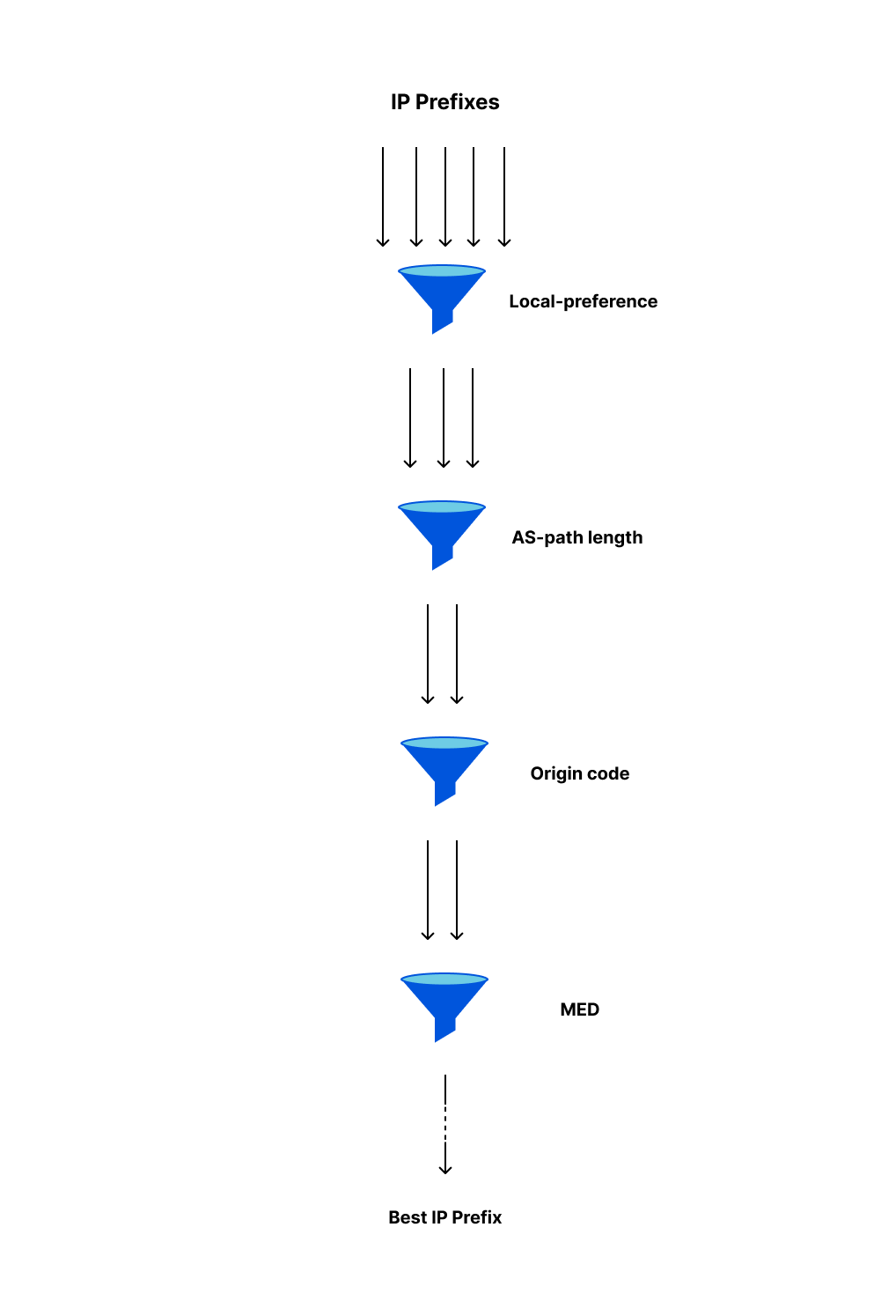
To understand the slowness that can often lead to BGP zombies, we need to talk about path hunting. Path hunting occurs when routers running BGP exhaustively search for the best path to a prefix as determined by Longest Prefix Matching (LPM) and BGP routing attributes like path length and local preference. This becomes relevant in our observations of exactly how routes become stuck, for how long they become stuck, and how visible they are on the Internet.
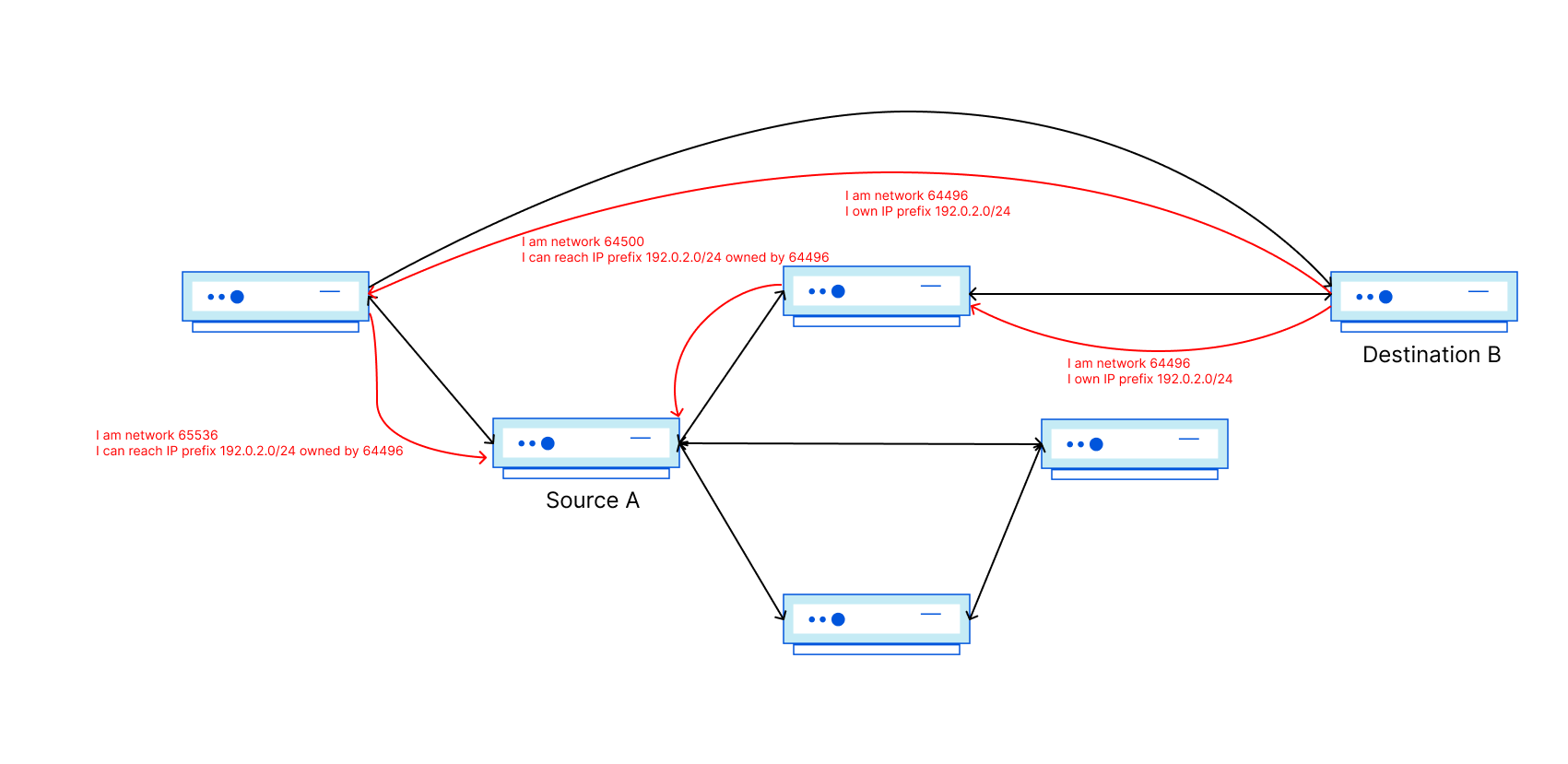
For example, path hunting happens when a more-specific BGP prefix is withdrawn from the global routing table, and networks need to fallback to a less-specific BGP advertisement. In this example, we use 2001:db8::/48 for the more-specific BGP announcement and 2001:db8::/32 for the less-specific prefix. When the /48 is withdrawn by the originating Autonomous System (AS), BGP routers have to recognize that route as missing and begin routing traffic to IPs such as 2001:db8::1 via the 2001:db8::/32 route, which still remains while the prefix 2001:db8::/48 is gone.
Let’s see what this could look like in action with a few diagrams.
Diagram 1: Active 2001:db8::/48 route
In this initial state, 2001:db8::/48 is used actively for traffic forwarding, which all flows through AS13335 on the way to AS64511. In this case, AS64511 would be a BYOIP customer of Cloudflare. AS64511 also announces a backup route to another Internet Service Provider (ISP), AS64510, but this route is not active even in AS64510’s routing table for forwarding to 2001:db8::1 because 2001:db8::/48 is a longer prefix match when compared to 2001:db8::/32.
Things get more interesting when AS64510 signals for 2001:db8::/48 to be withdrawn by Cloudflare (AS13335), perhaps because a DDoS attack is over and the customer opts to use Cloudflare only when they are actively under attack.
When the customer signals to Cloudflare (via BGP Control or API call) to withdraw the 2001:db8::/48 announcement, all BGP routers have to converge upon this update, which involves path hunting. AS13335 sends a BGP withdrawal message for 2001:db8::/48 to its directly-connected BGP neighbors. While the news of withdrawal may travel quickly from AS13335 to the other networks, news may travel more quickly to some of the neighbors than others. This means that until everyone has received and processed the withdrawal, networks may try routing through one another to reach the 2001:db8::/48 prefix – even after AS13335 has withdrawn it.
Diagram 2: 2001:db8::/48 route withdrawn via AS13335
Imagine AS64501 is a little slower than the rest – perhaps due to using older hardware, hardware being overloaded, a software bug, specific configuration settings, poor luck, or some other factor – and still has not processed the withdrawal of the /48. This in itself could be a BGP zombie, since the route is stuck for a small period. Our pings toward 2001:db8::1 are never able to actually reach AS64511, because AS13335 knows the /48 is meant to be withdrawn, but some routers carrying a full table have not yet converged upon that result.
The length of time spent path hunting is amplified by something called the Minimum Route Advertisement Interval (MRAI). The MRAI specifies the minimum amount of time between BGP advertisement messages from a BGP router, meaning it introduces a purposeful number of seconds of delay between each BGP advertisement update. RFC4271 recommends an MRAI value of 30-seconds for eBGP updates, and while this can cut down on the chattiness of BGP, or even potential oscillation of updates, it also makes path hunting take longer.
At the next cycle of path hunting, even AS64501, which was previously still pointing toward a nonexistent /48 route from AS13335, should find the /32 advertisement is all that is left toward 2001:db8::1. Once it has done so, the traffic flow will become the following:
Diagram 3: Routing fallback to 2001:db8::/32 and 2001:db8::/48 is gone from DFZ
This would mean BGP path hunting is over, and the Internet has realized that the 2001:db8::/32 is the best route available toward 2001:db8::1, and that 2001:db8::/48 is really gone. While in this example we’ve purposely made path hunting only last two cycles, in reality it can be far more, especially with how highly connected AS13335 is to thousands of peer networks and Tier-1’s globally.
Now that we’ve discussed BGP path hunting and how it works, you can probably already see how a BGP zombie outbreak can begin and how routing tables can become stuck for a lengthy period of time. Excessive BGP path hunting for a previously-known more-specific prefix can be an early indicator that a zombie could follow.
Spawning a zombie
Zombies have captured our attention more recently as they were noticed by some of our customers leveraging Bring-Your-Own-IP (BYOIP) on-demand advertisement for Magic Transit. BYOIP may be configured in two modes: “always-on”, in which a prefix is continuously announced, or “on-demand”, where a prefix is announced only when a customer chooses to. For some on-demand customers, announcement and withdrawal cycles may be a more frequent occurrence, which can lead to an increase in BGP zombies.
With that in mind and also knowing how path hunting works, let’s spawn our own zombie onto the Internet. To do so, we’ll take a spare block of IPv4 and IPv6 and announce them like so:
Once the routes are announced and stable, we’ll then proceed to withdraw the more specific routes advertised via Cloudflare globally. With a few quick clicks, we’ve successfully re-animated the dead.
Variant A: Ghoulish Gateways
One place zombies commonly occur is between upstream ISPs. When one router in a given ISP’s network is a little slower to update, routes can become stuck.
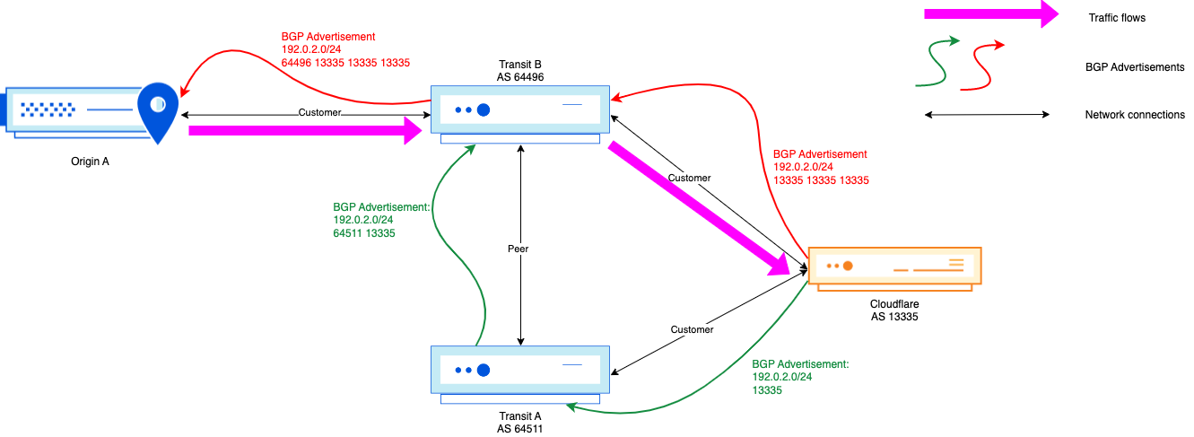
Take, for example, the following loop we observed between two of our upstream partners:
Simultaneously, zombies can occur entirely within a given network. When a route is withdrawn from Cloudflare’s network, each device in our network must individually begin the process of withdrawing the route. While this is generally a smooth process, things can still become stuck.
Take, for instance, a situation where one router inside of our network has not yet fully processed the withdrawal. Connectivity partners will continue routing traffic towards that router (as they have not yet received the withdrawal) while no host remains behind the router which is capable of actually processing the traffic. The result is an internal-only looping path:
Unlike most fictionally-depicted hoards of the walking dead, our highly-visible zombie has a limited lifetime in most major networks – in this instance, only around around 6 minutes, after which most had re-converged around the less-specific as the best path. Sadly, this is on the shorter side – in some cases, we have seen long-lived zombies cause reachability issues for more than 10 minutes. It’s safe to say this is longer than most network operators would expect BGP convergence to take in a normal situation.
But, you may ask – is this the excessive path hunting we talked about earlier, or a BGP zombie? Really, it depends on the expectation and tolerance around how long BGP convergence should take to process the prefix withdrawal. In any case, even over 30 minutes after our withdrawal of our more-specific prefix, we are able to see zombie routes in the route-views public collectors easily:
You might argue that six to eleven minutes (or more) is a reasonable time for worst-case BGP convergence in the Tier-1 network layer, though that itself seems like a stretch. Even setting that aside, our data shows that very real BGP zombies exist in the global routing table, and they will negatively impact traffic. Curiously, we observed the path hunting delay is worse on IPv4, with the longest observed IPv6 impact in major (Tier-1) networks being just over 4 minutes. One could speculate this is in part due to the much higher number of IPv4 prefixes in the Internet global routing table than the IPv6 global table, and how BGP speakers handle them separately.
Source: RIPEstat’s BGPlay
Part of the delay appears to originate from how interconnected AS13335 is; being heavily peered with a large portion of the Internet increases the likelihood of a route becoming stuck in a given location. Given that, perhaps a zombie would be shorter-lived if we operated in the opposite direction: announcing a less-specific persistently to 13335 and announcing more specifics via our local ISP during normal operation. Since the withdrawal will come from what is likely a less well-peered network, the time-to-convergence may be shorter:
Indeed, as predicted, we still get a stuck route, and it only lives for around 20 seconds in the Tier-1 network layer:
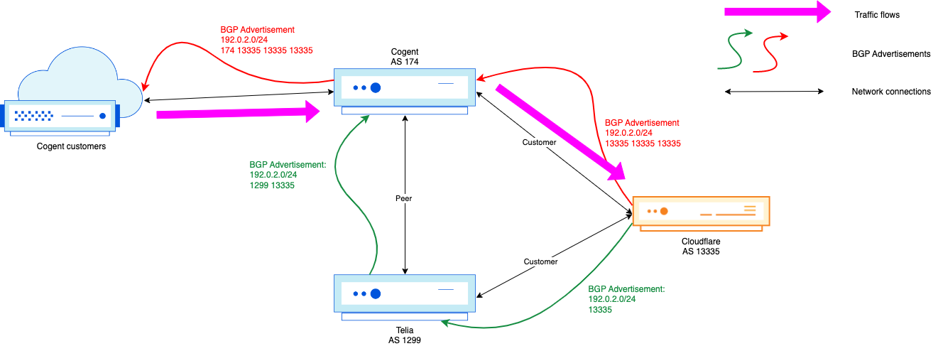
19. be12488.ccr42.ams03.atlas.cogentco.com
20. 38.88.214.142
21. be2020.ccr41.ams03.atlas.cogentco.com
22. 38.88.214.142
23. (waiting for reply)
24. 38.88.214.142
25. (waiting for reply)
26. 38.88.214.142
Unfortunately, that 20 seconds is still an impactful 20 seconds – while better, it’s not where we want to be. The exact length of time will depend on the native ISP networks one is connected with, and it could certainly ease into the minutes worth of stuck routing.
In both cases, the initial time-to-announce yielded no loss, nor was a zombie created, as both paths remained valid for the entirety of their initial lifetime. Zombies were only created when a more specific prefix was fully withdrawn. A newly-announced route is not subject to path hunting in the same way a withdrawn more-specific route is. As they say, good (new) news travels fast.
Lessening the zombie outbreak
Our findings lead us to believe that the withdrawal of a more-specific prefix may lead to zombies running rampant for longer periods of time. Because of this, we are exploring some improvements that make the consequences of BGP zombie routing less impactful for our customers relying on our on-demand BGP functionality.
For the traffic that does reach Cloudflare with stuck routes, we will introduce some BGP traffic forwarding improvements internally that allow for a more graceful withdrawal of traffic, even if routes are erroneously pointing toward us. In many ways, this will closely resemble the BGP well-known no-export community’s functionality from our servers running BGP. This means even if we receive traffic from external parties due to stuck routing, we will still have the opportunity to deliver traffic to our far-end customers over a tunneled connection or via a Cloudflare Network Interconnect (CNI). We look forward to reporting back the positive impact after making this improvement for a more graceful draining of traffic by default.
For the traffic that does not reach Cloudflare’s edge, and instead loops between network providers, we need to use a different approach. Since we know more-specific to less-specific prefix routing fallback is more prone to BGP zombie outbreak, we are encouraging customers to instead use a multi-step draining process when they want traffic drained from the Cloudflare edge for an on-demand prefix without introducing route loops or blackhole events. The draining process when removing traffic for a BYOIP prefix from Cloudflare should look like this:
The customer is already announcing an example prefix from Cloudflare, ex. 198.18.0.0/24
The customer begins natively announcing the prefix 198.18.0.0/24 (i.e. the same-length as the prefix they are advertising via Cloudflare) from their network to the Internet Service Providers that they wish to fail over traffic to.
After a few minutes, the customer signals BGP withdrawal from Cloudflare for the 198.18.0.0/24 prefix.
The result is a clean cut over: impactful zombies are avoided because the same-length prefix (198.18.0.0/24) remains in the global routing table. Excessive path hunting is avoided because instead of routers needing to aggressively seek out a missing more-specific prefix match, they can fallback to the same-length announcement that persists in the routing table from the natively-originated path to the customer’s network.
Source: RIPEstat’s BGPlay
What next?
We are going to continue to refine our methods of measuring BGP zombies, so you can look forward to more insights in the future. There is also work from others in the community around zombie measurement that is interesting and producing useful data. In terms of combatting the software bugs around BGP zombie creation, routing vendors should implement RFC9687, the BGP SendHoldTimer. The general idea is that a local router can detect via the SendHoldTimer if the far-end router stops processing BGP messages unexpectedly, which lowers the possibility of zombies becoming stuck for long periods of time.
In addition, it’s worth keeping in mind our observations made in this post about more-specific prefix announcements and excessive path hunting. If as a network operator you rely on more-specific BGP prefix announcements for failover, or for traffic engineering, you need to be aware that routes could become stuck for a longer period of time before full BGP convergence occurs.
If you’re interested in problems like BGP zombies, consider coming to work at Cloudflare or applying for an internship. Together we can help build a better Internet!
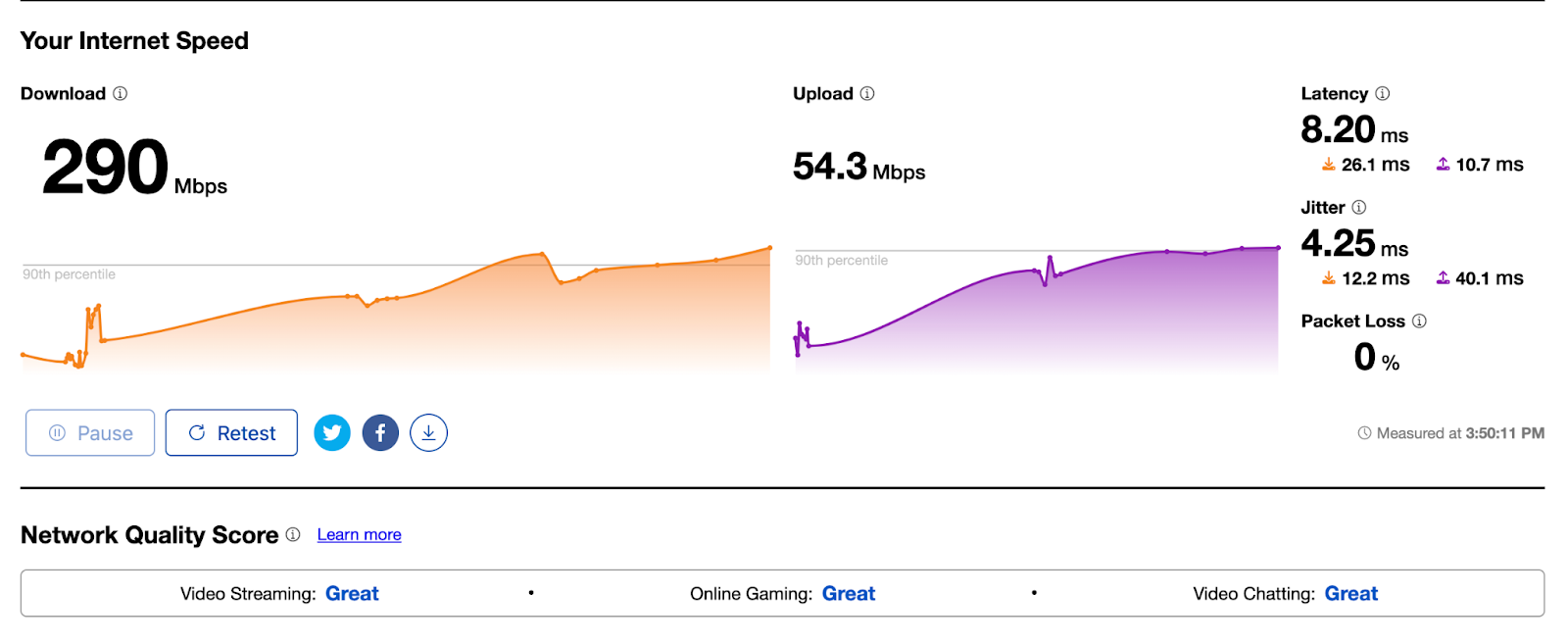
As the Internet has become enmeshed in our everyday lives, so has our need for speed. No one wants to wait when adding shoes to our shopping carts, or accessing corporate assets from across the globe. And as the Internet supports more and more of our critical infrastructure, speed becomes more than just a measure of how quickly we can place a takeout order. It becomes the connective tissue between the systems that keep us safe, healthy, and organized. Governments, financial institutions, healthcare ecosystems, transit — they increasingly rely on the Internet. This is why at Cloudflare, building the fastest network is our north star.
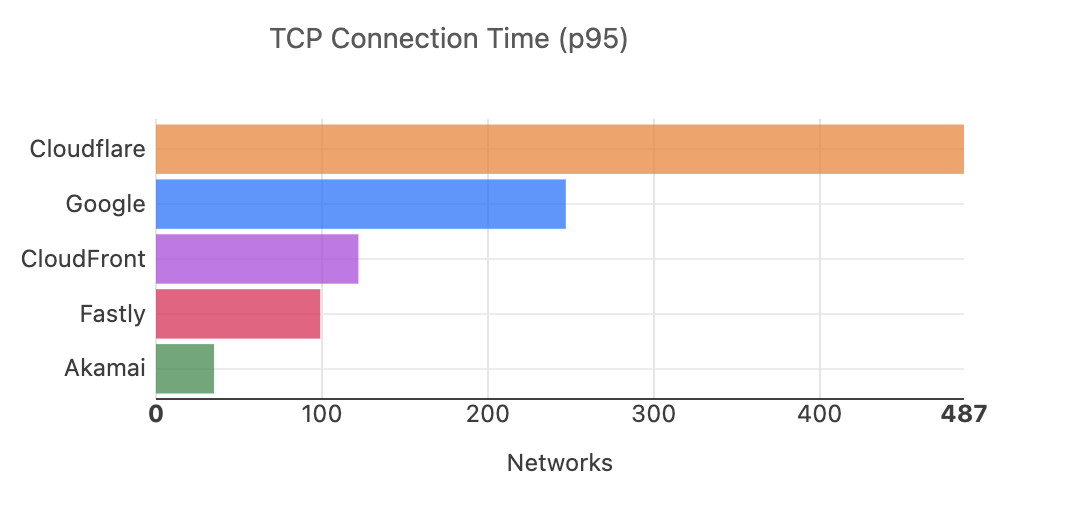
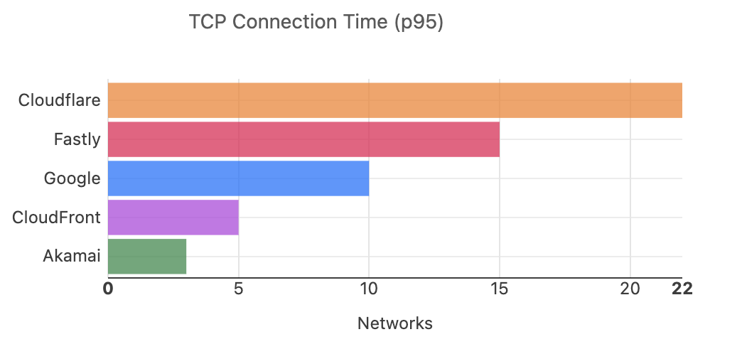
We’re happy to announce that we are the fastest network in 48% of the top 1000 networks by 95th percentile TCP connection time between November 2024, and March 2025, up from 44% in September 2024.
In this post, we’re going to share with you how our network performance has changed since our last post in September 2024, and talk about what makes us faster than other networks. But first, let’s talk a little bit about how we get this data.
How does Cloudflare get this data?
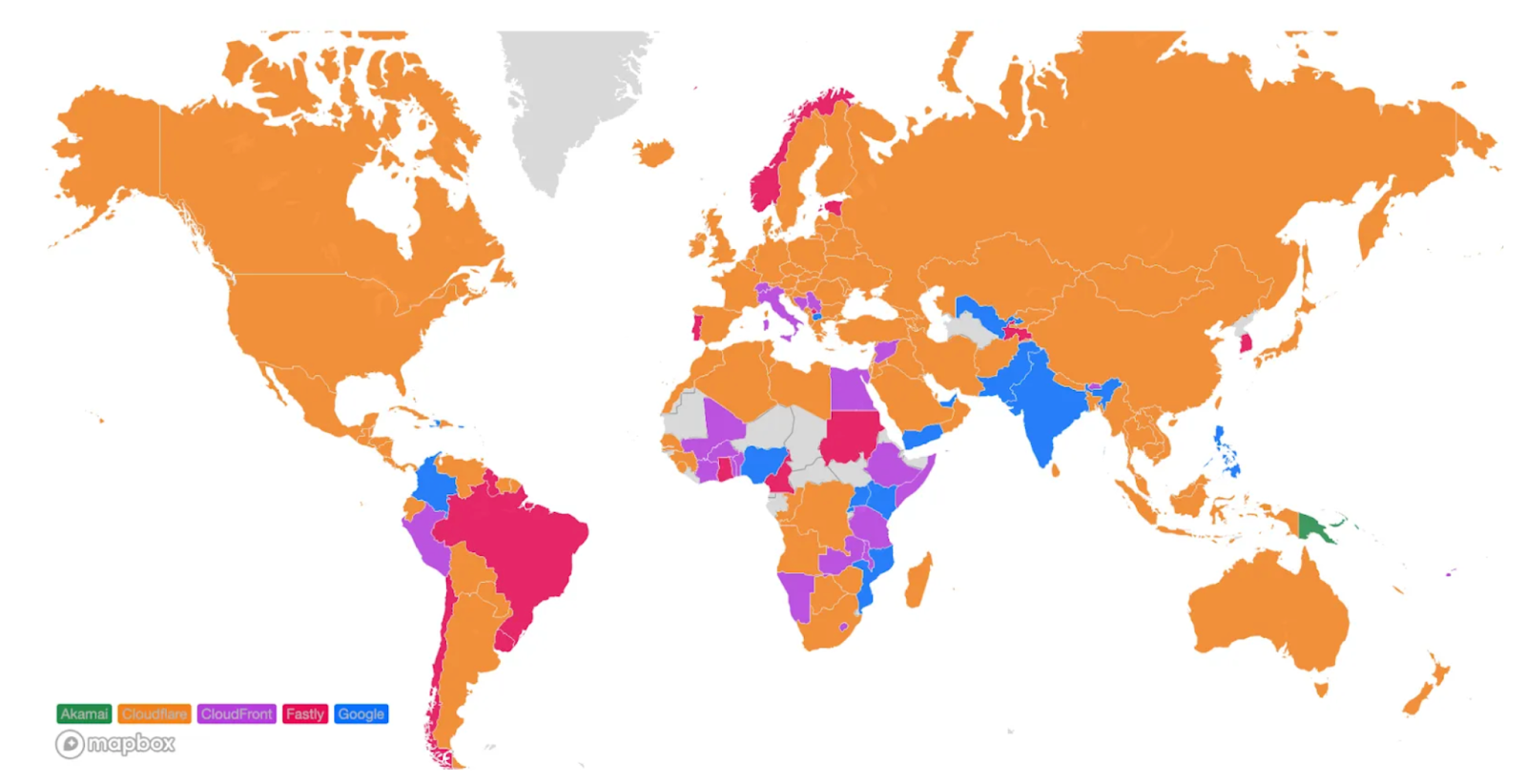
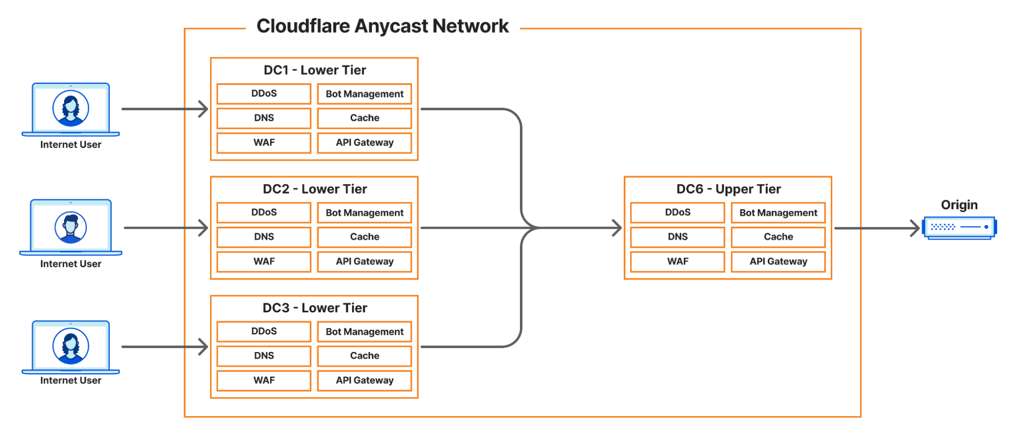
It’s happened to all of us — you casually click on a site, and suddenly you’ve reached a Cloudflare-branded error page. While you are shaking your fist at the sky, something interesting is happening on the back end. Cloudflare is using Real User Monitoring (RUM) to collect the data used to compare our performance against other networks. The monitoring we do is slightly different than the RUM Cloudflare offers to customers. When the error page loads, a 100 KB file is fetched and loaded. This file is hosted on networks like Cloudflare, Akamai, Amazon CloudFront, Fastly, and Google Cloud CDN. Your browser processes the performance data, and sends it to Cloudflare, where we use it to get a clear view of how these different networks stack up in terms of speed.
We’ve been collecting and refining this data since June 2021. You can read more about how we collect that data here, and we regularly track our performance during Innovation Weeks to hold ourselves accountable to you that we are always in pursuit of being the fastest network in the world.
How are we doing?
In order to evaluate Cloudflare’s speed relative to others, we measure performance across the top 1000 “eyeball” networks using the list provided by the Asia Pacific Network Information Centre (APNIC). So-called “eyeball” networks are those with a large concentration of subscribers/end users. This information is important, because it gives us signals for where we can expand our presence or peering, or optimize our traffic engineering. When benchmarking, we assess the 95th percentile TCP connection time. This is the time it takes a user to establish a TCP connection to the server they are trying to reach. This metric helps us illustrate how Cloudflare’s network makes your traffic faster by serving your customers as locally as possible.
When we look at Cloudflare’s performance across the top 1000 networks, we can see that we’re fastest in 487, or over 48%, of these networks, between November 2024 and March 2025:
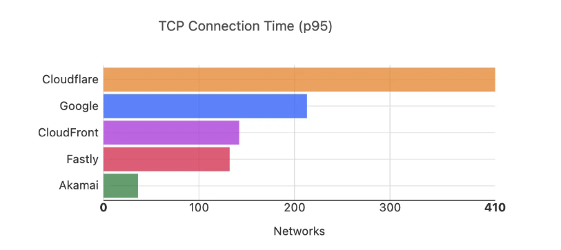
In September 2024, we ranked #1 in 44% of these networks:
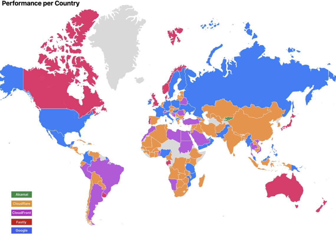
So why did we jump? To get a better understanding of why, let’s take a look at the countries where we improved, which will give us a better sense of where to dive in. This is what our network map looked like in September 2024 (grey countries mean we do not have enough data or users to derive insights):
(September 2024)
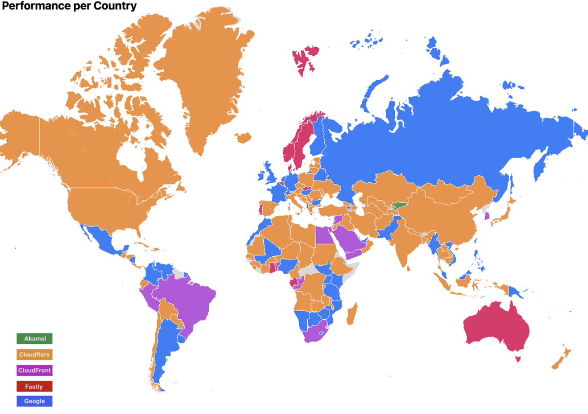
Today, using those same 95th percentile TCP connect times, we rank #1 in 48% of networks and the network map looks like this:
(March 2025)
We made most of our gains in Africa, where countries that previously didn’t have enough samples saw an increase in samples, and Cloudflare pulled ahead. This could mean that there was either an increase in Cloudflare users, or an increase in error pages shown. These countries got faster almost exclusively due to the presence of our Edge Partner deployments, which are Cloudflare locations embedded in last mile networks. In next-generation markets like many African countries, these locations are crucial towards being faster as connectivity to end users tends to fall back to places like South Africa or London if in-country peering does not exist.
But let’s take a look at a couple of other places and see why we got faster.
In Canada, we were not the fastest in September 2024, but we are the fastest today. Today, we are the fastest in 40% of networks, which is the most out of all of our competitors:
But when you look at the overall country numbers, we see that the race for the fastest network is quite close:
Canada 95th Percentile TCP Connect Time by Provider
Rank
Entity
Connect Time (P95)
#1 Diff
1
Cloudflare
179 ms
–
2
Fastly
180 ms
+0.48% (+0.87 ms)
3
Google
180 ms
+0.74% (+1.32 ms)
4
CloudFront
182 ms
+1.74% (+3.11 ms)
5
Akamai
215 ms
+20% (+36 ms)
The difference between Cloudflare and the third-fastest network is a little over a millisecond! As we’ve pointed out previously, such fluctuations are quite common, especially at higher percentiles. But there is still a significant difference between us and the slowest network; we’re around 20% faster.
However, looking at a place like Japan where were not the fastest in September 2024 but are now the fastest, there is a significant difference between Cloudflare and the number two network:
Japan 95th Percentile TCP Connect Time by Provider
Rank
Entity
Connect Time (P95)
#1 Diff
1
Cloudflare
116 ms
–
2
Fastly
122 ms
+5.23% (+6.08 ms)
3
Google
124 ms
+6.21% (+7.22 ms)
4
CloudFront
127 ms
+8.91% (+10 ms)
5
Akamai
153 ms
+32% (+37 ms)
Why is this? We are in more locations in Japan than our competitors and added more Edge Partner deployments in these locations, bringing us even closer to end-users. Edge Partner deployments are collaborations with ISPs, where we take space in their data centers, and peer with them directly.
Why?
Why do we track our network performance like this? The answer is simple: to improve user experience. This data allows us to track a key performance metric for Cloudflare and the other networks. When we see that we’re lagging in a region, it serves as a signal to dig deeper into our network.
This data is a gold mine for the teams tasked with improving Cloudflare’s network. When there are countries where Cloudflare is behind, it gives us signals for where we should expand or investigate. If we’re slow, we may need to invest in additional peering. If a region we have invested in heavily is slower, we may need to investigate our hardware. The example from Japan shows exactly how this can benefit: we took a location where we were previously on par with our competitors, added peering in new locations, and we pulled ahead.
On top of this map, we have autonomous system (ASN) level granularity on how we are performing on each one of the top 1000 eyeball networks, and we continuously optimize our traffic flow with each of them. This allows us to track individual networks that may lag and improve the customer experience in those networks through turning up peering, or even adding new deployments in those regions.
What’s next?
We’re sharing our updates on our journey to become #1 everywhere so that you can see what goes into running the fastest network in the world. From here, our plan is the same as always: identify where we’re slower, fix it, and then tell you how we’ve gotten faster.
Cloudflare was recently contacted by a group of anonymous security researchers who discovered a broadcast amplification vulnerability through their QUIC Internet measurement research. Our team collaborated with these researchers through our Public Bug Bounty program, and worked to fully patch a dangerous vulnerability that affected our infrastructure.
Since being notified about the vulnerability, we’ve implemented a mitigation to help secure our infrastructure. According to our analysis, we have fully patched this vulnerability and the amplification vector no longer exists.
Summary of the amplification attack
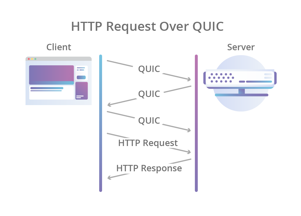
QUIC is an Internet transport protocol that is encrypted by default. It offers equivalent features to TCP (Transmission Control Protocol) and TLS (Transport Layer Security), while using a shorter handshake sequence that helps reduce connection establishment times. QUIC runs over UDP (User Datagram Protocol).
The researchers found that a single client QUIC Initial packet targeting a broadcast IP destination address could trigger a large response of initial packets. This manifested as both a server CPU amplification attack and a reflection amplification attack.
Transport and security handshakes
When using TCP and TLS there are two handshake interactions. First, is the TCP 3-way transport handshake. A client sends a SYN packet to a server, it responds with a SYN-ACK to the client, and the client responds with an ACK. This process validates the client IP address. Second, is the TLS security handshake. A client sends a ClientHello to a server, it carries out some cryptographic operations and responds with a ServerHello containing a server certificate. The client verifies the certificate, confirms the handshake and sends application traffic such as an HTTP request.
QUIC follows a similar process, however the sequence is shorter because the transport and security handshake is combined. A client sends an Initial packet containing a ClientHello to a server, it carries out some cryptographic operations and responds with an Initial packet containing a ServerHello with a server certificate. The client verifies the certificate and then sends application data.
The QUIC handshake does not require client IP address validation before starting the security handshake. This means there is a risk that an attacker could spoof a client IP and cause a server to do cryptographic work and send data to a target victim IP (aka a reflection attack). RFC 9000 is careful to describe the risks this poses and provides mechanisms to reduce them (for example, see Sections 8 and 9.3.1). Until a client address is verified, a server employs an anti-amplification limit, sending a maximum of 3x as many bytes as it has received. Furthermore, a server can initiate address validation before engaging in the cryptographic handshake by responding with a Retry packet. The retry mechanism, however, adds an additional round-trip to the QUIC handshake sequence, negating some of its benefits compared to TCP. Real-world QUIC deployments use a range of strategies and heuristics to detect traffic loads and enable different mitigations.
In order to understand how the researchers triggered an amplification attack despite these QUIC guardrails, we first need to dive into how IP broadcast works.
Broadcast addresses
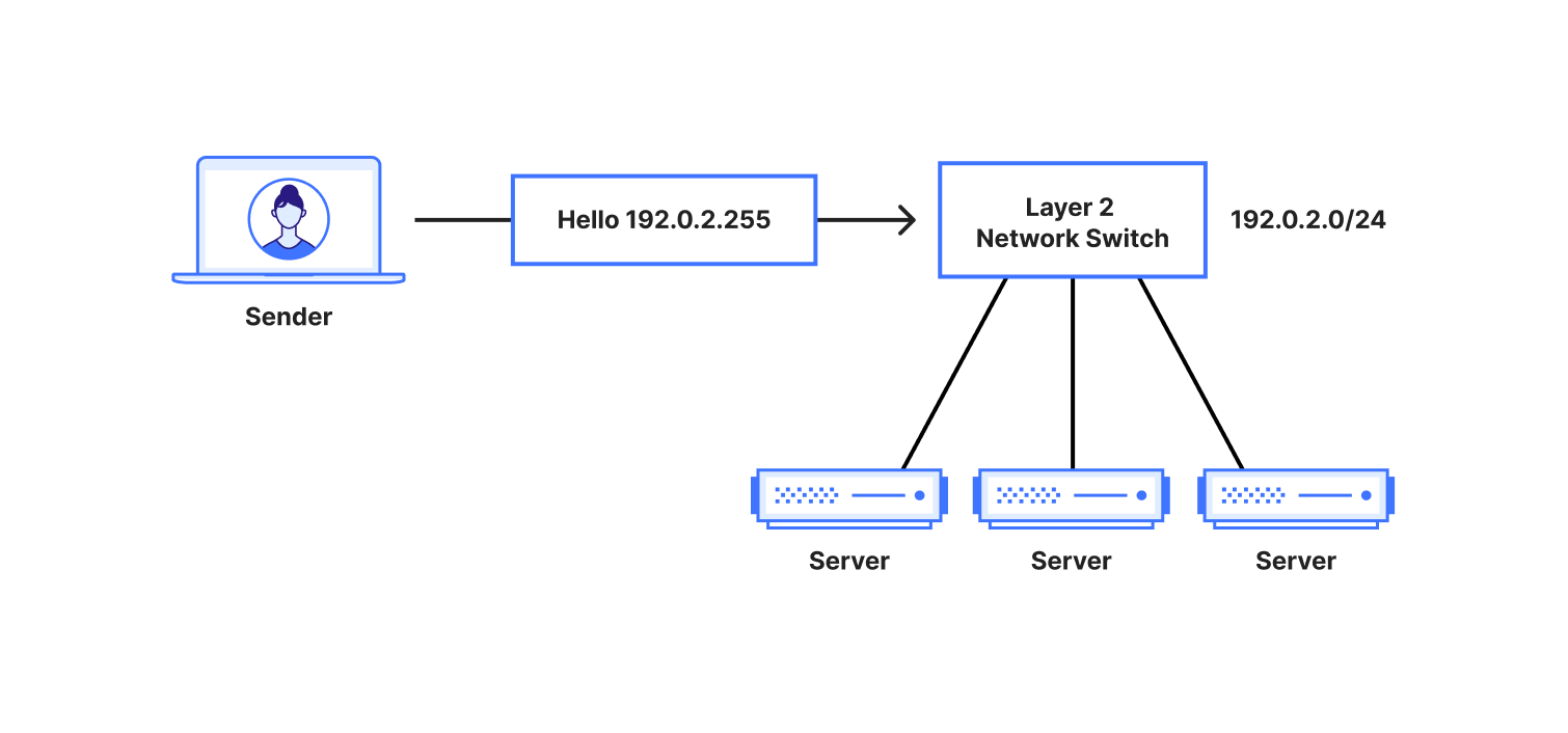
In Internet Protocol version 4 (IPv4) addressing, the final address in any given subnet is a special broadcast IP address used to send packets to every node within the IP address range. Every node that is within the same subnet receives any packet that is sent to the broadcast address, enabling one sender to send a message that can be “heard” by potentially hundreds of adjacent nodes. This behavior is enabled by default in most network-connected systems and is critical for discovery of devices within the same IPv4 network.
The broadcast address by nature poses a risk of DDoS amplification; for every one packet sent, hundreds of nodes have to process the traffic.
Dealing with the expected broadcast
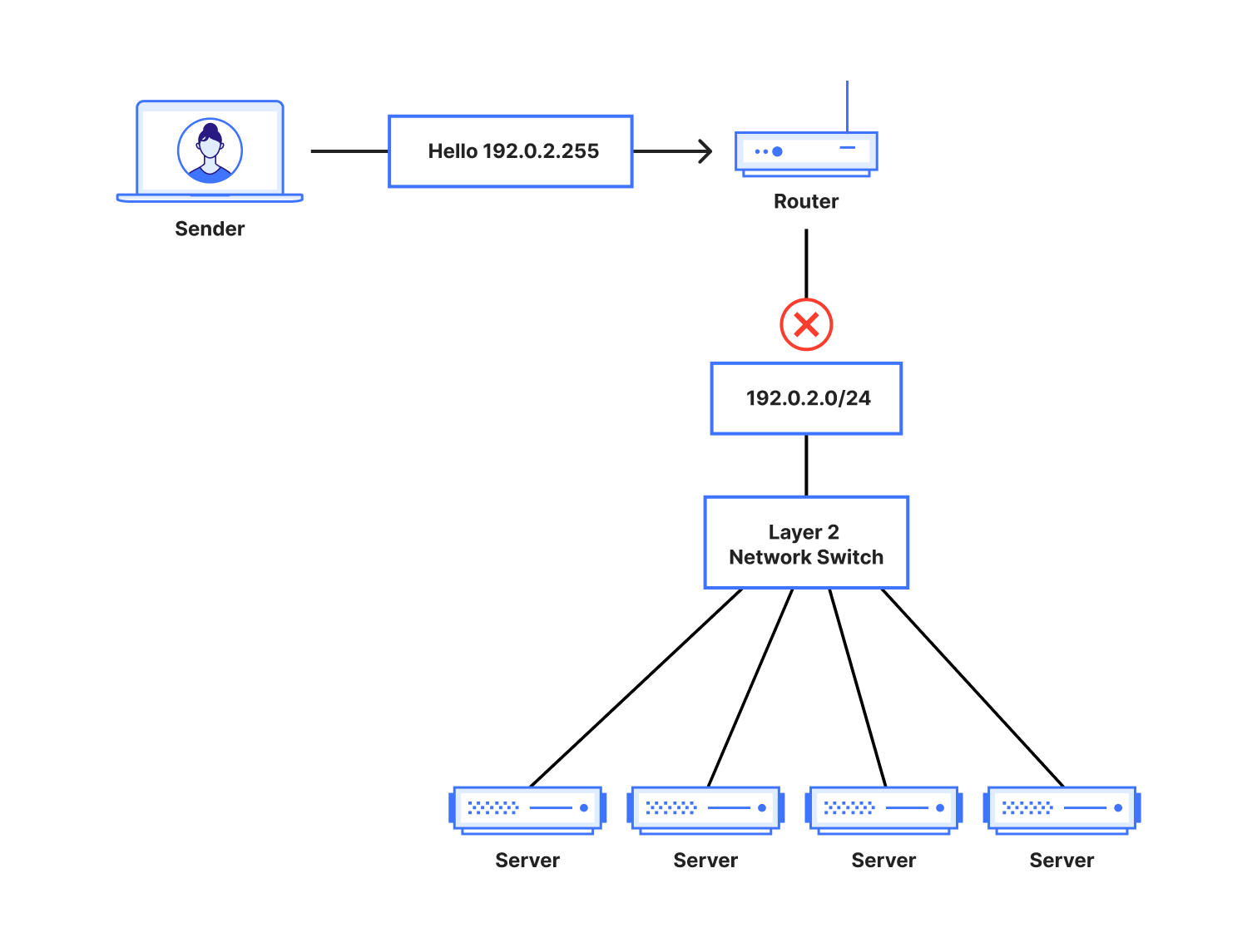
To combat the risk posed by broadcast addresses, by default most routers reject packets originating from outside their IP subnet which are targeted at the broadcast address of networks for which they are locally connected. Broadcast packets are only allowed to be forwarded within the same IP subnet, preventing attacks from the Internet from targeting servers across the world.
The same techniques are not generally applied when a given router is not directly connected to a given subnet. So long as an address is not locally treated as a broadcast address, Border Gateway Protocol (BGP) or other routing protocols will continue to route traffic from external IPs toward the last IPv4 address in a subnet. Essentially, this means a “broadcast address” is only relevant within a local scope of routers and hosts connected together via Ethernet. To routers and hosts across the Internet, a broadcast IP address is routed in the same way as any other IP.
Binding IP address ranges to hosts
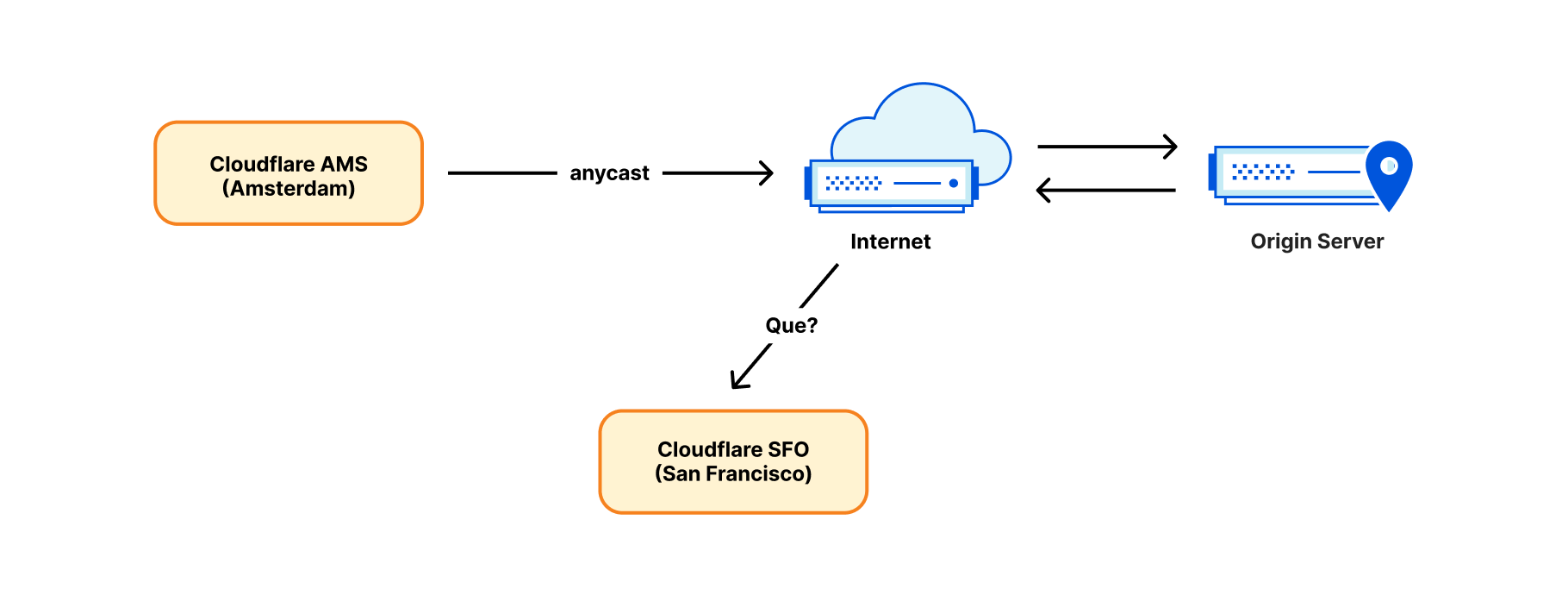
Each Cloudflare server is expected to be capable of serving content from every website on the Cloudflare network. Because our network utilizes Anycast routing, each server necessarily needs to be listening on (and capable of returning traffic from) every Anycast IP address in use on our network.
To do so, we take advantage of the loopback interface on each server. Unlike a physical network interface, all IP addresses within a given IP address range are made available to the host (and will be processed locally by the kernel) when bound to the loopback interface.
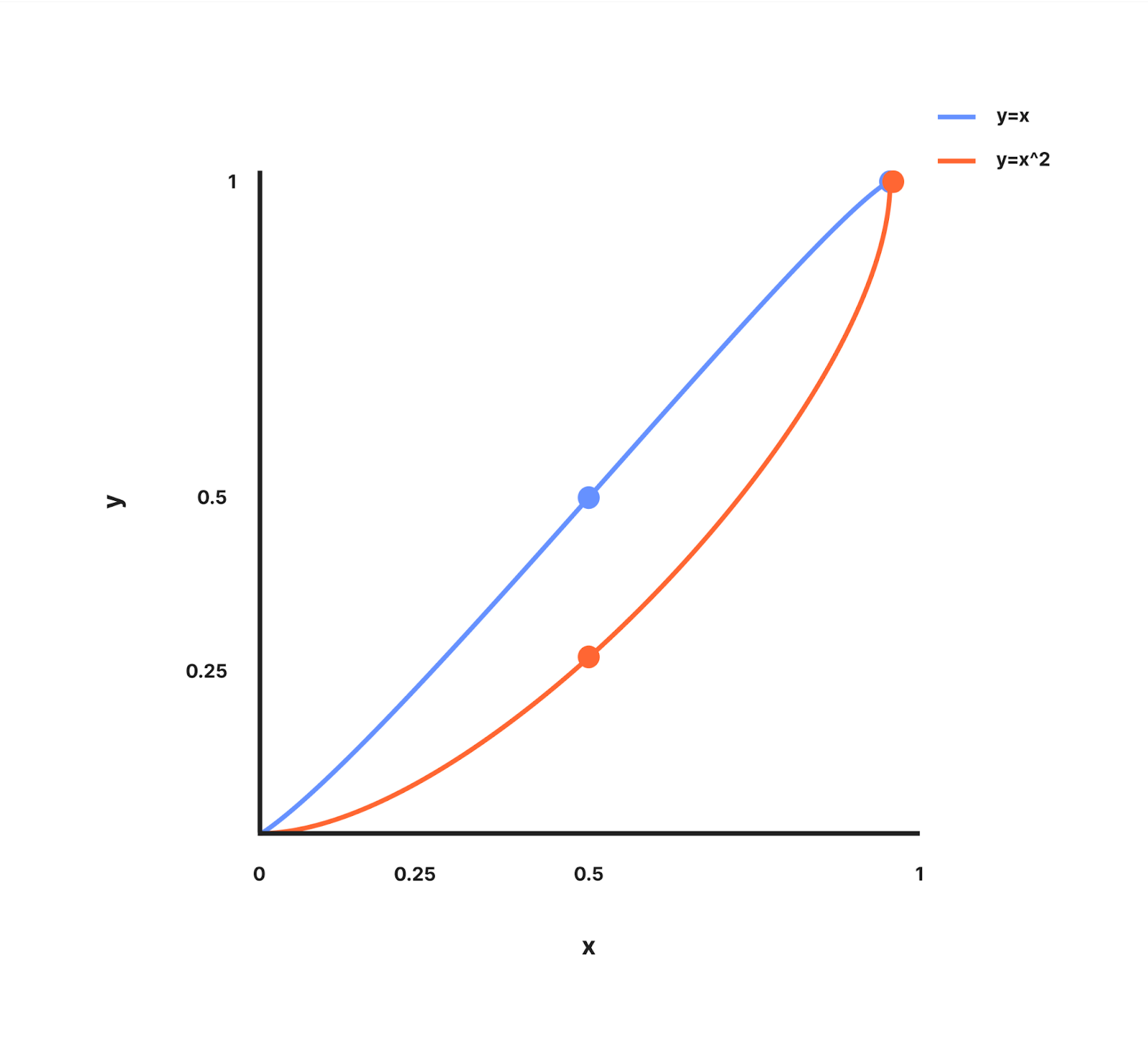
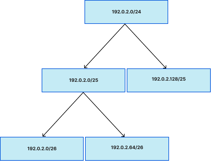
The mechanism by which this works is straightforward. In a traditional routing environment, longest prefix matching is employed to select a route. Under longest prefix matching, routes towards more specific blocks of IP addresses (such as 192.0.2.96/29, a range of 8 addresses) will be selected over routes to less specific blocks of IP addresses (such as 192.0.2.0/24, a range of 256 addresses).
While Linux utilizes longest prefix matching, it consults an additional step — the Routing Policy Database (RPDB) — before immediately searching for a match. The RPDB contains a list of routing tables which can contain routing information and their individual priorities. The default RPDB looks like this:
$ ip rule show
0:	from all lookup local
32766:	from all lookup main
32767:	from all lookup default
Linux will consult each routing table in ascending numerical order to try and find a matching route. Once one is found, the search is terminated and the route immediately used.
If you’ve previously worked with routing rules on Linux, you are likely familiar with the contents of the main table. Contrary to the existence of the table named “default”, “main” generally functions as the default lookup table. It is also the one which contains what we traditionally associate with route table information:
$ ip route show table main
default via 192.0.2.1 dev eth0 onlink
192.0.2.0/24 dev eth0 proto kernel scope link src 192.0.2.2
This is, however, not the first routing table that will be consulted for a given lookup. Instead, that task falls to the local table:
$ ip route show table local
local 127.0.0.0/8 dev lo proto kernel scope host src 127.0.0.1
local 127.0.0.1 dev lo proto kernel scope host src 127.0.0.1
broadcast 127.255.255.255 dev lo proto kernel scope link src 127.0.0.1
local 192.0.2.2 dev eth0 proto kernel scope host src 192.0.2.2
broadcast 192.0.2.255 dev eth0 proto kernel scope link src 192.0.2.2
Looking at the table, we see two new types of routes — local and broadcast. As their names would suggest, these routes dictate two distinctly different functions: routes that are handled locally and routes that will result in a packet being broadcast. Local routes provide the desired functionality — any prefix with a local route will have all IP addresses in the range processed by the kernel. Broadcast routes will result in a packet being broadcast to all IP addresses within the given range. Both types of routes are added automatically when an IP address is bound to an interface (and, when a range is bound to the loopback (lo) interface, the range itself will be added as a local route).
Vulnerability discovery
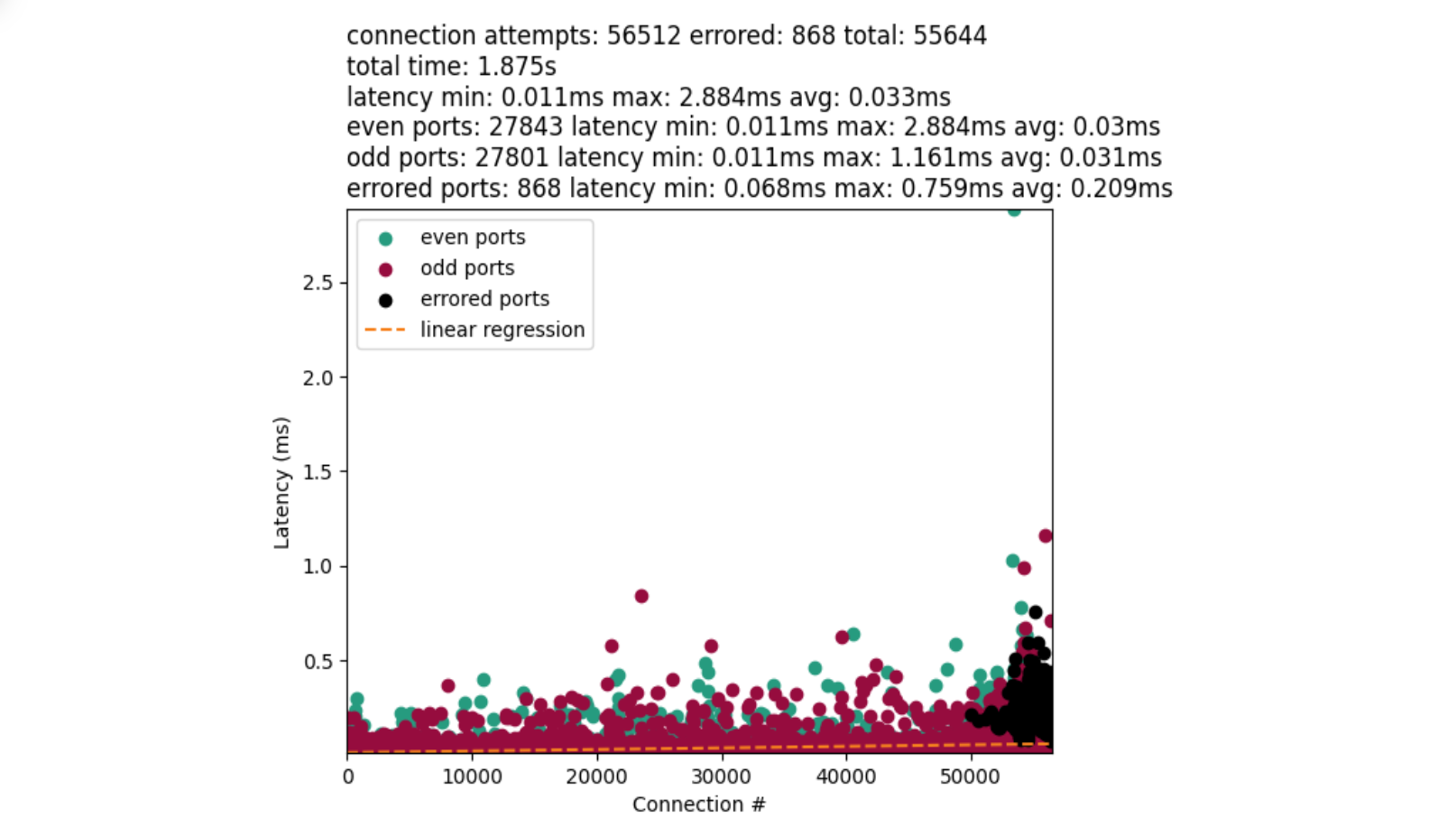
Deployments of QUIC are highly dependent on the load-balancing and packet forwarding infrastructure that they sit on top of. Although QUIC’s RFCs describe risks and mitigations, there can still be attack vectors depending on the nature of server deployments. The reporting researchers studied QUIC deployments across the Internet and discovered that sending a QUIC Initial packet to one of Cloudflare’s broadcast addresses triggered a flood of responses. The aggregate amount of response data exceeded the RFC’s 3x amplification limit.
Taking a look at the local routing table of an example Cloudflare system, we see a potential culprit:
$ ip route show table local
local 127.0.0.0/8 dev lo proto kernel scope host src 127.0.0.1
local 127.0.0.1 dev lo proto kernel scope host src 127.0.0.1
broadcast 127.255.255.255 dev lo proto kernel scope link src 127.0.0.1
local 192.0.2.2 dev eth0 proto kernel scope host src 192.0.2.2
broadcast 192.0.2.255 dev eth0 proto kernel scope link src 192.0.2.2
local 203.0.113.0 dev lo proto kernel scope host src 203.0.113.0
local 203.0.113.0/24 dev lo proto kernel scope host src 203.0.113.0
broadcast 203.0.113.255 dev lo proto kernel scope link src 203.0.113.0
On this example system, the anycast prefix 203.0.113.0/24 has been bound to the loopback interface (lo) through the use of standard tooling. Acting dutifully under the standards of IPv4, the tooling has assigned both special types of routes — a local one for the IP range itself and a broadcast one for the final address in the range — to the interface.
While traffic to the broadcast address of our router’s directly connected subnet is filtered as expected, broadcast traffic targeting our routed anycast prefixes still arrives at our servers themselves. Normally, broadcast traffic arriving at the loopback interface does little to cause problems. Services bound to a specific port across an entire range will receive data sent to the broadcast address and continue as normal. Unfortunately, this relatively simple trait breaks down when normal expectations are broken.
Cloudflare’s frontend consists of several worker processes, each of which independently binds to the entire anycast range on UDP port 443. In order to enable multiple processes to bind to the same port, we use the SO_REUSEPORT socket option. While SO_REUSEPORT has additional benefits, it also causes traffic sent to the broadcast address to be copied to every listener.
Each individual QUIC server worker operates in isolation. Each one reacted to the same client Initial, duplicating the work on the server side and generating response traffic to the client’s IP address. Thus, a single packet could trigger a significant amplification. While specifics will vary by implementation, a typical one-listener-per-core stack (which sends retries in response to presumed timeouts) on a 128-core system could result in 384 replies being generated and sent for each packet sent to the broadcast address.
Although the researchers demonstrated this attack on QUIC, the underlying vulnerability can affect other UDP request/response protocols that use sockets in the same way.
Mitigation
As a communication methodology, broadcast is not generally desirable for anycast prefixes. Thus, the easiest method to mitigate the issue was simply to disable broadcast functionality for the final address in each range.
Ideally, this would be done by modifying our tooling to only add the local routes in the local routing table, skipping the inclusion of the broadcast ones altogether. Unfortunately, the only practical mechanism to do so would involve patching and maintaining our own internal fork of the iproute2 suite, a rather heavy-handed solution for the problem at hand.
Instead, we decided to focus on removing the route itself. Similar to any other route, it can be removed using standard tooling:
$ sudo ip route del 203.0.113.255 table local
To do so at scale, we made a relatively minor change to our deployment system:
  {%- for lo_route in lo_routes %}
    {%- if lo_route.type == "broadcast" %}
        # All broadcast addresses are implicitly ipv4
        {%- do remove_route({
        "dev": "lo",
        "dst": lo_route.dst,
        "type": "broadcast",
        "src": lo_route.src,
        }) %}
    {%- endif %}
  {%- endfor %}
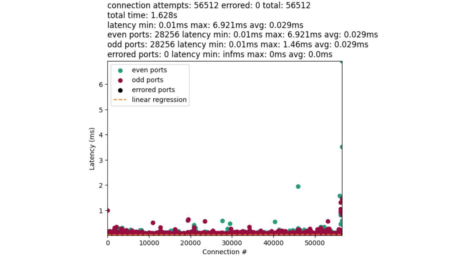
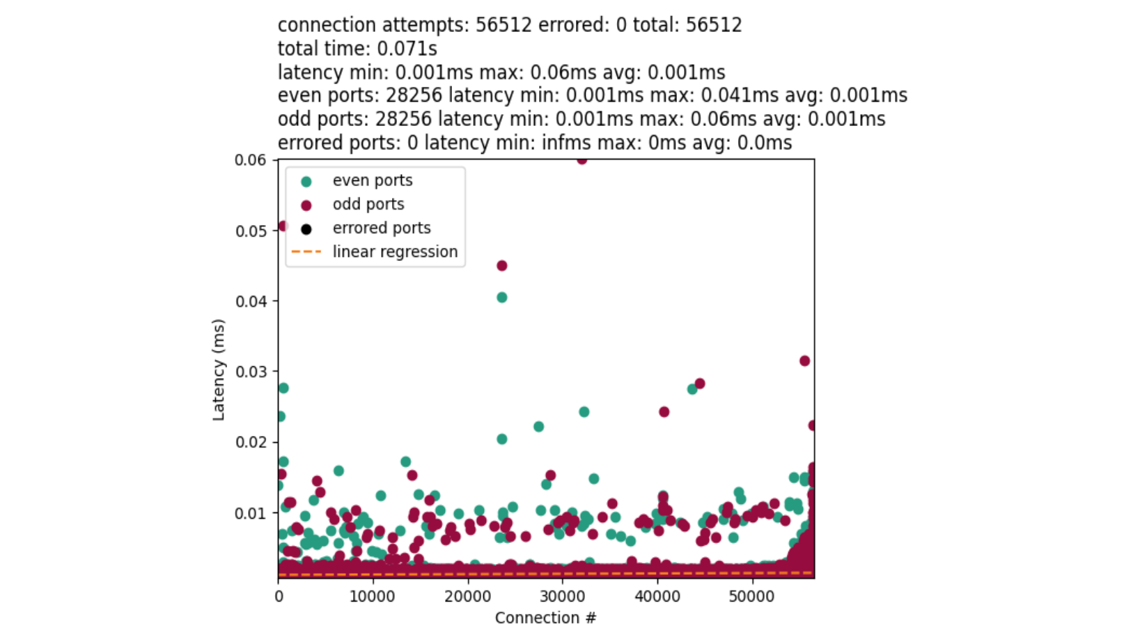
In doing so, we effectively ensure that all broadcast routes attached to the loopback interface are removed, mitigating the risk by ensuring that the specification-defined broadcast address is treated no differently than any other address in the range.
Next steps
While the vulnerability specifically affected broadcast addresses within our anycast range, it likely expands past our infrastructure. Anyone with infrastructure that meets the relatively narrow criteria (a multi-worker, multi-listener UDP-based service that is bound to all IP addresses on a machine with routable IP prefixes attached in such a way as to expose the broadcast address) will be affected unless mitigations are in place. We encourage network administrators and security professionals to assess their systems for configurations that may present a local amplification attack vector.
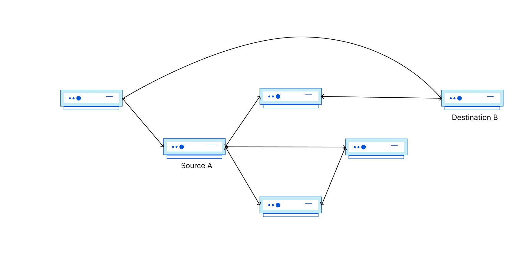
The Internet is designed to provide multiple paths between two endpoints. Attempts to exploit multi-path opportunities are almost as old as the Internet, culminating in RFCs documenting some of the challenges. Still, today, virtually all end-to-end communication uses only one available path at a time. Why? It turns out that in multi-path setups, even the smallest differences between paths can harm the connection quality due to packet reordering and other issues. As a result, Internet devices usually use a single path and let the routers handle the path selection.
There is another way. Enter Multi-Path TCP (MPTCP), which exploits the presence of multiple interfaces on a device, such as a mobile phone that has both Wi-Fi and cellular antennas, to achieve multi-path connectivity.
MPTCP has had a long history — see the Wikipedia article and the spec (RFC 8684) for details. It’s a major extension to the TCP protocol, and historically most of the TCP changes failed to gain traction. However, MPTCP is supposed to be mostly an operating system feature, making it easy to enable. Applications should only need minor code changes to support it.
There is a caveat, however: MPTCP is still fairly immature, and while it can use multiple paths, giving it superpowers over regular TCP, it’s not always strictly better than it. Whether MPTCP should be used over TCP is really a case-by-case basis.
In this blog post we show how to set up MPTCP to find out.
Subflows
Internally, MPTCP extends TCP by introducing “subflows”. When everything is working, a single TCP connection can be backed by multiple MPTCP subflows, each using different paths. This is a big deal – a single TCP byte stream is now no longer identified by a single 5-tuple. On Linux you can see the subflows with ss -M, like:
Here you can see a single MPTCP connection, composed of two underlying TCP flows.
MPTCP aspirations
Being able to separate the lifetime of a connection from the lifetime of a flow allows MPTCP to address two problems present in classical TCP: aggregation and mobility.
Aggregation: MPTCP can aggregate the bandwidth of many network interfaces. For example, in a data center scenario, it’s common to use interface bonding. A single flow can make use of just one physical interface. MPTCP, by being able to launch many subflows, can expose greater overall bandwidth. I’m personally not convinced if this is a real problem. As we’ll learn below, modern Linux has a BLESS-like MPTCP scheduler and macOS stack has the “aggregation” mode, so aggregation should work, but I’m not sure how practical it is. However, there are certainly projects that are trying to do link aggregation using MPTCP.
Mobility: On a customer device, a TCP stream is typically broken if the underlying network interface goes away. This is not an uncommon occurrence — consider a smartphone dropping from Wi-Fi to cellular. MPTCP can fix this — it can create and destroy many subflows over the lifetime of a single connection and survive multiple network changes.
Improving reliability for mobile clients is a big deal. While some software can use QUIC, which also works on Multipath Extensions, a large number of classical services still use TCP. A great example is SSH: it would be very nice if you could walk around with a laptop and keep an SSH session open and switch Wi-Fi networks seamlessly, without breaking the connection.
MPTCP work was initially driven by UCLouvain in Belgium. The first serious adoption was on the iPhone. Apparently, users have a tendency to use Siri while they are walking out of their home. It’s very common to lose Wi-Fi connectivity while they are doing this. (source)
Implementations
Currently, there are only two major MPTCP implementations — Linux kernel support from v5.6, but realistically you need at least kernel v6.1 (MPTCP is not supported on Android yet) and iOS from version 7 / Mac OS X from 10.10.
Typically, Linux is used on the server side, and iOS/macOS as the client. It’s possible to get Linux to work as a client-side, but it’s not straightforward, as we’ll learn soon. Beware — there is plenty of outdated Linux MPTCP documentation. The code has had a bumpy history and at least two different APIs were proposed. See the Linux kernel source for the mainline API and the mptcp.dev website.
Linux as a server
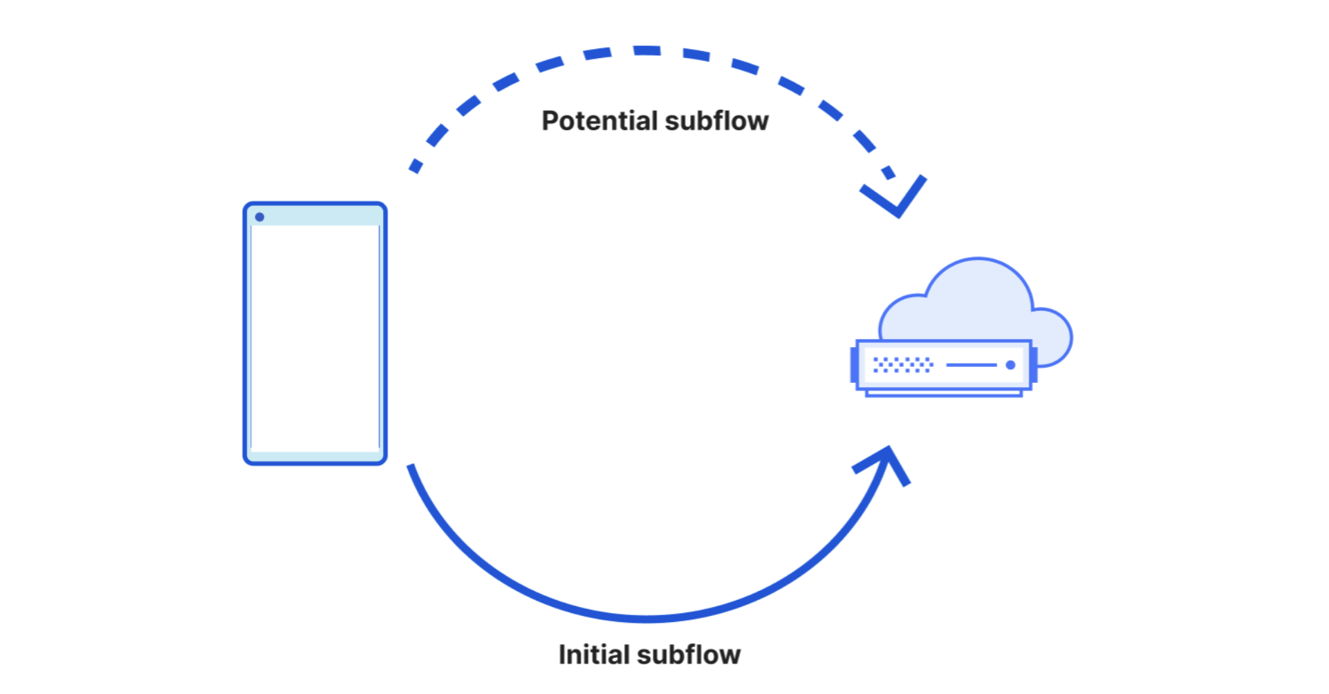
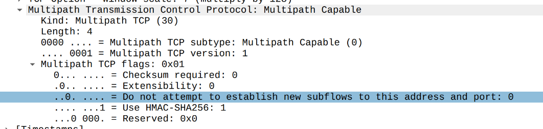
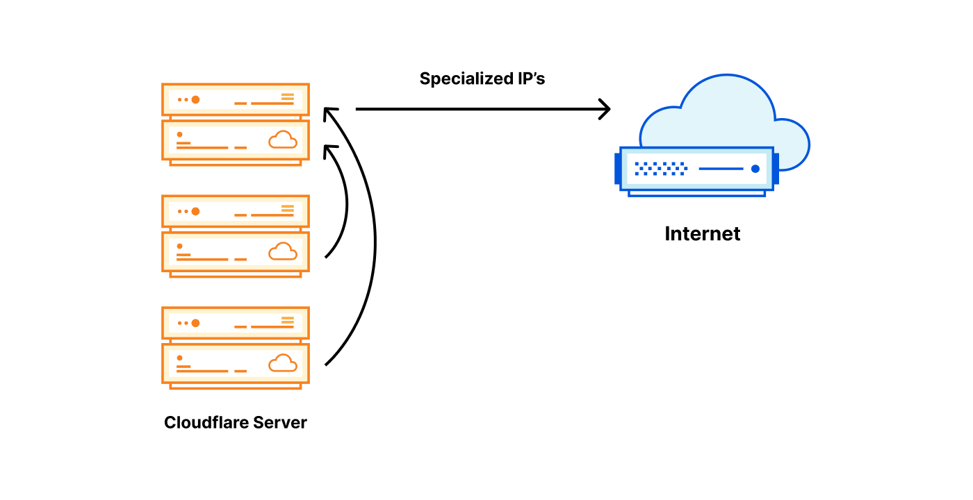
Conceptually, the MPTCP design is pretty sensible. After the initial TCP handshake, each peer may announce additional addresses (and ports) on which it can be reached. There are two ways of doing this. First, in the handshake TCP packet each peer specifies the “Do not attempt to establish new subflows to this address and port” bit, also known as bit [C], in the MPTCP TCP extensions header.
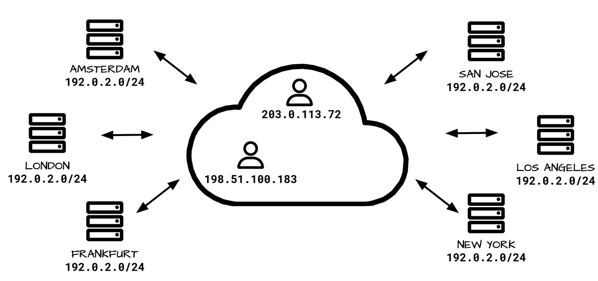
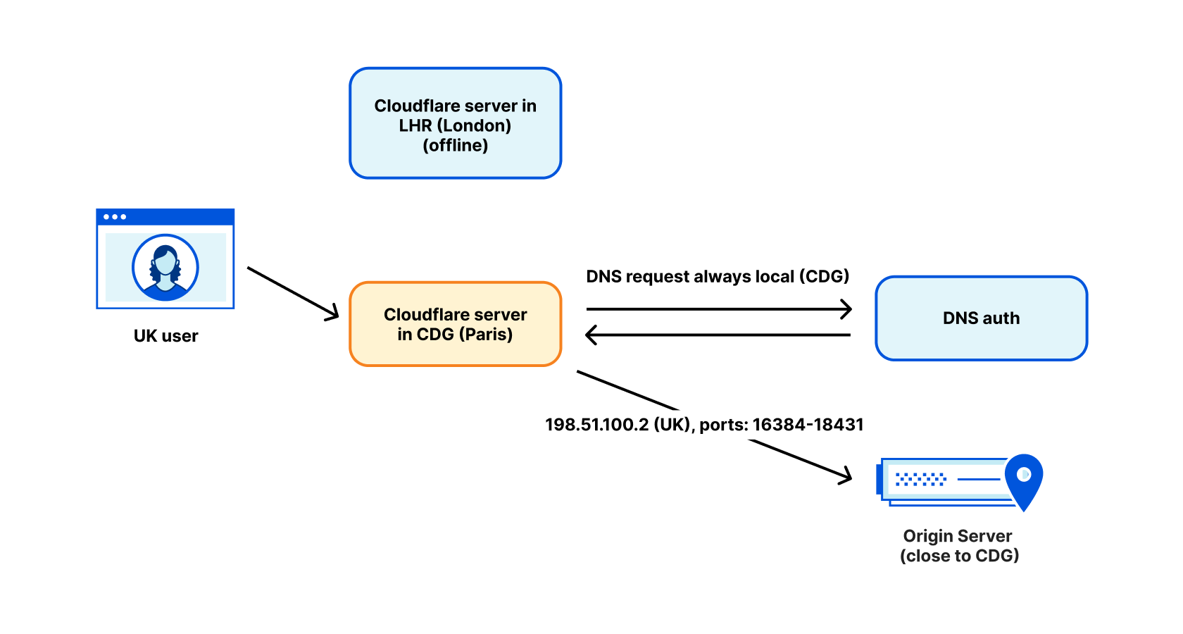
With this bit cleared, the other peer is free to assume the two-tuple is fine to be reconnected to. Typically, the server allows the client to reuse the server IP/port address. Usually, the client is not listening and disallows the server to connect back to it. There are caveats though. For example, in the context of Cloudflare, where our servers are using Anycast addressing, reconnecting to the server IP/port won’t work. Going twice to the IP/port pair is unlikely to reach the same server. For us it makes sense to set this flag, disallowing clients from reconnecting to our server addresses. This can be done on Linux with:
# Linux server sysctl - useful for ECMP or Anycast servers
$ sysctl -w net.mptcp.allow_join_initial_addr_port=0
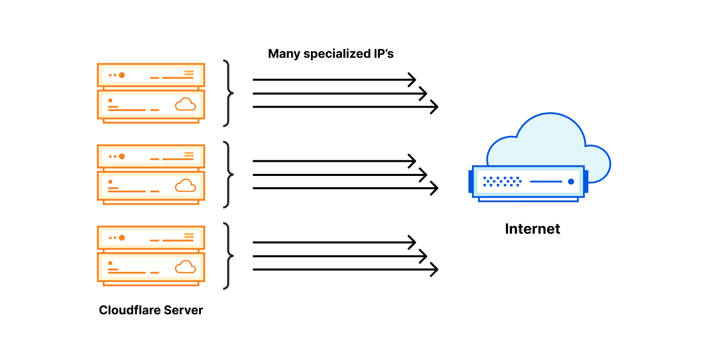
There is also a second way to advertise a listening IP/port. During the lifetime of a connection, a peer can send an ADD-ADDR MPTCP signal which advertises a listening IP/port. This can be managed on Linux by ip mptcp endpoint ... signal, like:
# Linux server - extra listening address
$ ip mptcp endpoint add 192.51.100.1 dev eth0 port 4321 signal
With such a config, a Linux peer (typically server) will report the additional IP/port with ADD-ADDR MPTCP signal in an ACK packet, like this:
It’s important to realize that either peer can send ADD-ADDR messages. Unusual as it might sound, it’s totally fine for the client to advertise extra listening addresses. The most common scenario though, consists of either nobody, or just a server, sending ADD-ADDR.
Technically, to launch an MPTCP socket on Linux, you just need to replace IPPROTO_TCP with IPPROTO_MPTCP in the application code:
In practice, though, this introduces some changes to the sockets API. Currently not all setsockopt’s work yet — like TCP_USER_TIMEOUT. Additionally, at this stage, MPTCP is incompatible with kTLS.
Path manager / scheduler
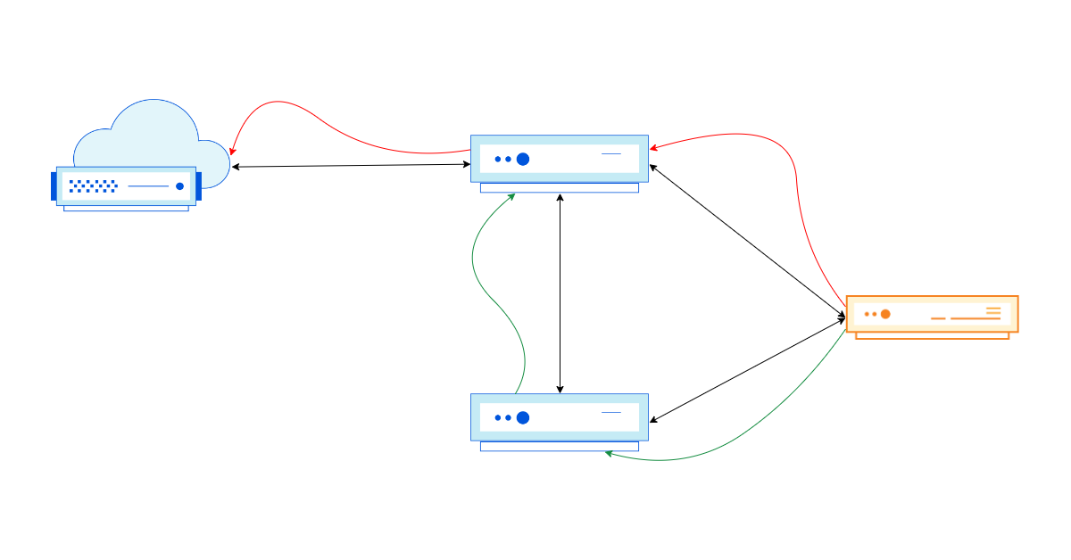
Once the peers have exchanged the address information, MPTCP is ready to kick in and perform the magic. There are two independent pieces of logic that MPTCP handles. First, given the address information, MPTCP must figure out if it should establish additional subflows. The component that decides on this is called “Path Manager”. Then, another component called “scheduler” is responsible for choosing a specific subflow to transmit the data over.
Both peers have a path manager, but typically only the client uses it. A path manager has a hard task to launch enough subflows to get the benefits, but not too many subflows which could waste resources. This is where the MPTCP stacks get complicated.
Linux as client
On Linux, path manager is an operating system feature, not an application feature. The in-kernel path manager requires some configuration — it must know which IP addresses and interfaces are okay to start new subflows. This is configured with ip mptcp endpoint ... subflow, like:
$ ip mptcp endpoint add dev wlp1s0 192.0.2.3 subflow # Linux client
This informs the path manager that we (typically a client) own a 192.0.2.3 IP address on interface wlp1s0, and that it’s fine to use it as source of a new subflow. There are two additional flags that can be passed here: “backup” and “fullmesh”. Maintaining these ip mptcp endpoints on a client is annoying. They need to be added and removed every time networks change. Fortunately, NetworkManager from 1.40 supports managing these by default. If you want to customize the “backup” or “fullmesh” flags, you can do this here (see the documentation):
ubuntu$ cat /etc/NetworkManager/conf.d/95-mptcp.conf
# set "subflow" on all managed "ip mptcp endpoints". 0x22 is the default.
[connection]
connection.mptcp-flags=0x22
Path manager also takes a “limit” setting, to set a cap of additional subflows per MPTCP connection, and limit the received ADD-ADDR messages, like:
$ ip mptcp limits set subflow 4 add_addr_accepted 2 # Linux client
I experimented with the “mobility” use case on my Ubuntu 22 Linux laptop. I repeatedly enabled and disabled Wi-Fi and Ethernet. On new kernels (v6.12), it works, and I was able to hold a reliable MPTCP connection over many interface changes. I was less lucky with the Ubuntu v6.8 kernel. Unfortunately, the default path manager on Linux client only works when the flag “Do not attempt to establish new subflows to this address and port” is cleared on the server. Server-announced ADD-ADDR don’t result in new subflows created, unless ip mptcp endpoint has a fullmesh flag.
It feels like the underlying MPTCP transport code works, but the path manager requires a bit more intelligence. With a new kernel, it’s possible to get the “interactive” case working out of the box, but not for the ADD-ADDR case.
Custom path manager
Linux allows for two implementations of a path manager component. It can either use built-in kernel implementation (default), or userspace netlink daemon.
$ sysctl -w net.mptcp.pm_type=1 # use userspace path manager
However, from what I found there is no serious implementation of configurable userspace path manager. The existing implementations don’t do much, and the API seemsimmature yet.
Scheduler and BPF extensions
Thus far we’ve covered Path Manager, but what about the scheduler that chooses which link to actually use? It seems that on Linux there is only one built-in “default” scheduler, and it can do basic failover on packet loss. The developers want to write MPTCP schedulers in BPF, and this work is in-progress.
macOS
As opposed to Linux, macOS and iOS expose a raw MPTCP API. On those operating systems, path manager is not handled by the kernel, but instead can be an application responsibility. The exposed low-level API is based on connectx(). For example, here’s an example of obscure code that establishes one connection with two subflows:
This powerful API is hard to use though, as it would require every application to listen for network changes. Fortunately, macOS and iOS also expose higher-level APIs. One example is nw_connection in C, which uses nw_parameters_set_multipath_service.
Another, more common example is using Network.framework, and would look like this:
let parameters = NWParameters.tcp
parameters.multipathServiceType = .interactive
let connection = NWConnection(host: host, port: port, using: parameters)
The API supports three MPTCP service type modes:
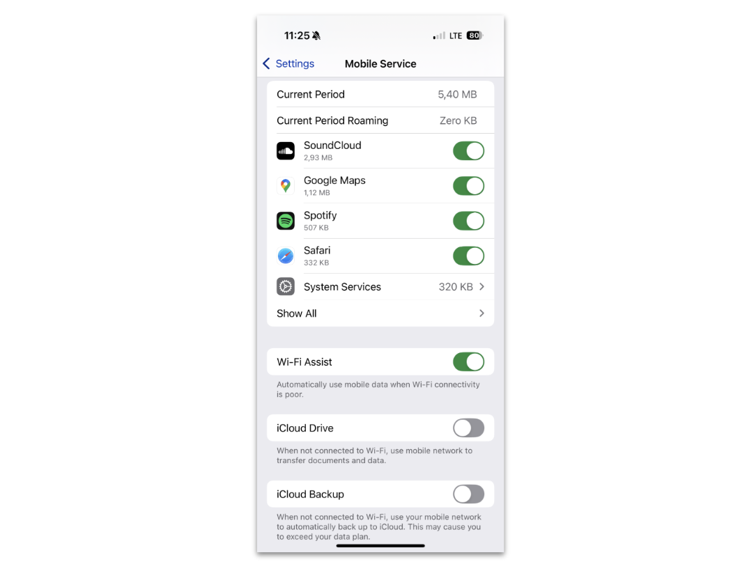
Handover Mode: Tries to minimize cellular. Uses only Wi-Fi. Uses cellular only when Wi-Fi Assist is enabled and makes such a decision.
Interactive Mode: Used for Siri. Reduces latency. Only for low-bandwidth flows.
Aggregation Mode: Enables resource pooling but it’s only available for developer accounts and not deployable.
The MPTCP API is nicely integrated with the iPhone “Wi-Fi Assist” feature. While the official documentation is lacking, it’s possible to find sources explaining how it actually works. I was able to successfully test both the cleared “Do not attempt to establish new subflows” bit and ADD-ADDR scenarios. Hurray!
IPv6 caveat
Sadly, MPTCP IPv6 has a caveat. Since IPv6 addresses are long, and MPTCP uses the space-constrained TCP Extensions field, there is not enough room for ADD-ADDR messages if TCP timestamps are enabled. If you want to use MPTCP and IPv6, it’s something to consider.
Summary
I find MPTCP very exciting, being one of a few deployable serious TCP extensions. However, current implementations are limited. My experimentation showed that the only practical scenario where currently MPTCP might be useful is:
Linux as a server
macOS/iOS as a client
“interactive” use case
With a bit of effort, Linux can be made to work as a client.
Don’t get me wrong, Linux developers did tremendous work to get where we are, but, in my opinion for any serious out-of-the-box use case, we’re not there yet. I’m optimistic that Linux can develop a good MPTCP client story relatively soon, and the possibility of implementing the Path manager and Scheduler in BPF is really enticing.
Time will tell if MPTCP succeeds — it’s been 15 years in the making. In the meantime, Multi-Path QUIC is under active development, but it’s even further from being usable at this stage.
We’re not quite sure if it makes sense for Cloudflare to support MPTCP. Reach out if you have a use case in mind!
Shoutout to Matthieu Baerts for tremendous help with this blog post.
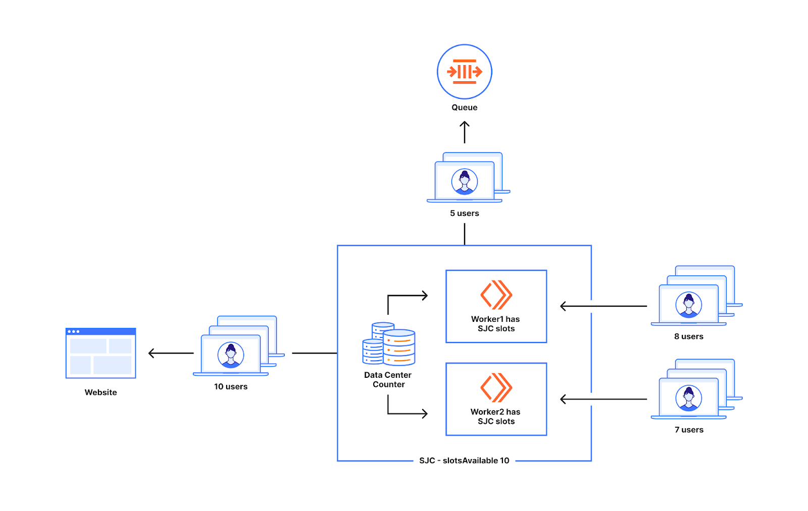
Netflix operates a highly efficient cloud computing infrastructure that supports a wide array of applications essential for our SVOD (Subscription Video on Demand), live streaming and gaming services. Utilizing Amazon AWS, our infrastructure is hosted across multiple geographic regions worldwide. This global distribution allows our applications to deliver content more effectively by serving traffic closer to our customers. Like any distributed system, our applications occasionally require data synchronization between regions to maintain seamless service delivery.
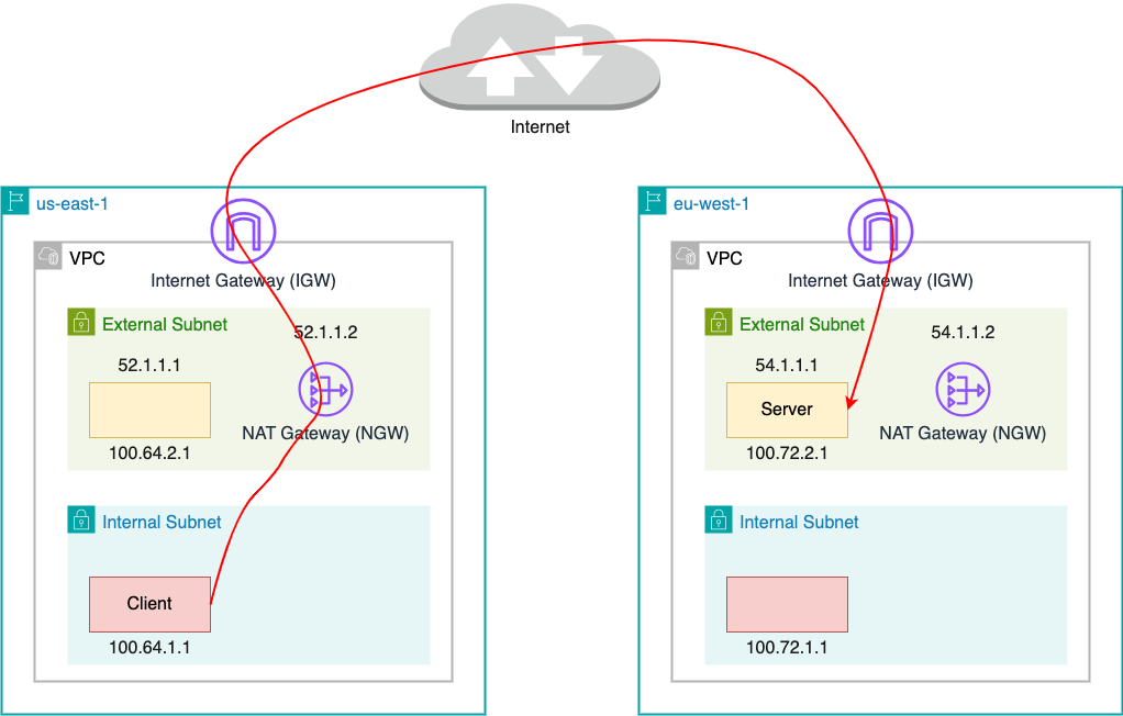
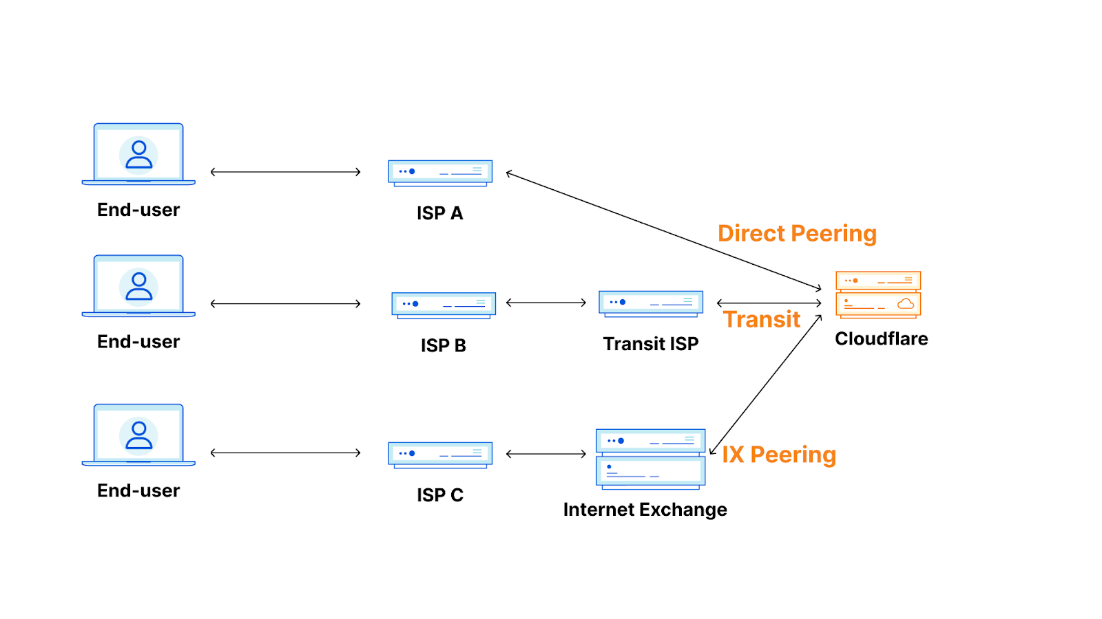
The following diagram shows a simplified cloud network topology for cross-region traffic.
The Problem At First Glance
Our Cloud Network Engineering on-call team received a request to address a network issue affecting an application with cross-region traffic. Initially, it appeared that the application was experiencing timeouts, likely due to suboptimal network performance. As we all know, the longer the network path, the more devices the packets traverse, increasing the likelihood of issues. For this incident, the client application is located in an internal subnet in the US region while the server application is located in an external subnet in a European region. Therefore, it is natural to blame the network since packets need to travel long distances through the internet.
As network engineers, our initial reaction when the network is blamed is typically, “No, it can’t be the network,” and our task is to prove it. Given that there were no recent changes to the network infrastructure and no reported AWS issues impacting other applications, the on-call engineer suspected a noisy neighbor issue and sought assistance from the Host Network Engineering team.
Blame the Neighbors
In this context, a noisy neighbor issue occurs when a container shares a host with other network-intensive containers. These noisy neighbors consume excessive network resources, causing other containers on the same host to suffer from degraded network performance. Despite each container having bandwidth limitations, oversubscription can still lead to such issues.
Upon investigating other containers on the same host — most of which were part of the same application — we quickly eliminated the possibility of noisy neighbors. The network throughput for both the problematic container and all others was significantly below the set bandwidth limits. We attempted to resolve the issue by removing these bandwidth limits, allowing the application to utilize as much bandwidth as necessary. However, the problem persisted.
Blame the Network
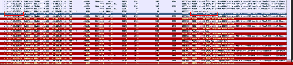
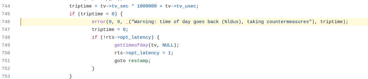
We observed some TCP packets in the network marked with the RST flag, a flag indicating that a connection should be immediately terminated. Although the frequency of these packets was not alarmingly high, the presence of any RST packets still raised suspicion on the network. To determine whether this was indeed a network-induced issue, we conducted a tcpdump on the client. In the packet capture file, we spotted one TCP stream that was closed after exactly 30 seconds.
SYN at 18:47:06
After the 3-way handshake (SYN,SYN-ACK,ACK), the traffic started flowing normally. Nothing strange until FIN at 18:47:36 (30 seconds later)
The packet capture results clearly indicated that it was the client application that initiated the connection termination by sending a FIN packet. Following this, the server continued to send data; however, since the client had already decided to close the connection, it responded with RST packets to all subsequent data from the server.
To ensure that the client wasn’t closing the connection due to packet loss, we also conducted a packet capture on the server side to verify that all packets sent by the server were received. This task was complicated by the fact that the packets passed through a NAT gateway (NGW), which meant that on the server side, the client’s IP and port appeared as those of the NGW, differing from those seen on the client side. Consequently, to accurately match TCP streams, we needed to identify the TCP stream on the client side, locate the raw TCP sequence number, and then use this number as a filter on the server side to find the corresponding TCP stream.
With packet capture results from both the client and server sides, we confirmed that all packets sent by the server were correctly received before the client sent a FIN.
Now, from the network point of view, the story is clear. The client initiated the connection requesting data from the server. The server kept sending data to the client with no problem. However, at a certain point, despite the server still having data to send, the client chose to terminate the reception of data. This led us to suspect that the issue might be related to the client application itself.
Blame the Application
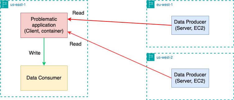
In order to fully understand the problem, we now need to understand how the application works. As shown in the diagram below, the application runs in the us-east-1 region. It reads data from cross-region servers and writes the data to consumers within the same region. The client runs as containers, whereas the servers are EC2 instances.
Notably, the cross-region read was problematic while the write path was smooth. Most importantly, there is a 30-second application-level timeout for reading the data. The application (client) errors out if it fails to read an initial batch of data from the servers within 30 seconds. When we increased this timeout to 60 seconds, everything worked as expected. This explains why the client initiated a FIN — because it lost patience waiting for the server to transfer data.
Could it be that the server was updated to send data more slowly? Could it be that the client application was updated to receive data more slowly? Could it be that the data volume became too large to be completely sent out within 30 seconds? Sadly, we received negative answers for all 3 questions from the application owner. The server had been operating without changes for over a year, there were no significant updates in the latest rollout of the client, and the data volume had remained consistent.
Blame the Kernel
If both the network and the application weren’t changed recently, then what changed? In fact, we discovered that the issue coincided with a recent Linux kernel upgrade from version 6.5.13 to 6.6.10. To test this hypothesis, we rolled back the kernel upgrade and it did restore normal operation to the application.
Honestly speaking, at that time I didn’t believe it was a kernel bug because I assumed the TCP implementation in the kernel should be solid and stable (Spoiler alert: How wrong was I!). But we were also out of ideas from other angles.
There were about 14k commits between the good and bad kernel versions. Engineers on the team methodically and diligently bisected between the two versions. When the bisecting was narrowed to a couple of commits, a change with “tcp” in its commit message caught our attention. The final bisecting confirmed that this commit was our culprit.
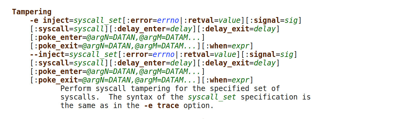
Interestingly, while reviewing the email history related to this commit, we found that another user had reported a Python test failure following the same kernel upgrade. Although their solution was not directly applicable to our situation, it suggested that a simpler test might also reproduce our problem. Using strace, we observed that the application configured the following socket options when communicating with the server:
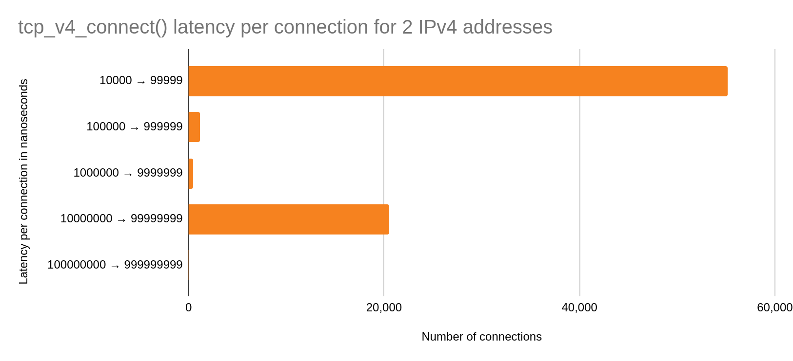
We then developed a minimal client-server C application that transfers a file from the server to the client, with the client configuring the same set of socket options. During testing, we used a 10M file, which represents the volume of data typically transferred within 30 seconds before the client issues a FIN. On the old kernel, this cross-region transfer completed in 22 seconds, whereas on the new kernel, it took 39 seconds to finish.
The Root Cause
With the help of the minimal reproduction setup, we were ultimately able to pinpoint the root cause of the problem. In order to understand the root cause, it’s essential to have a grasp of the TCP receive window.
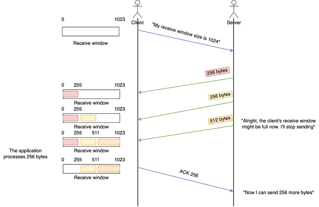
TCP Receive Window
Simply put, the TCP receive window is how the receiver tells the sender “This is how many bytes you can send me without me ACKing any of them”. Assuming the sender is the server and the receiver is the client, then we have:
The Window Size
Now that we know the TCP receive window size could affect the throughput, the question is, how is the window size calculated? As an application writer, you can’t decide the window size, however, you can decide how much memory you want to use for buffering received data. This is configured using SO_RCVBUF socket option we saw in the strace result above. However, note that the value of this option means how much application data can be queued in the receive buffer. In man 7 socket, there is
SO_RCVBUF
Sets or gets the maximum socket receive buffer in bytes. The kernel doubles this value (to allow space for bookkeeping overhead) when it is set using setsockopt(2), and this doubled value is returned by getsockopt(2). The default value is set by the /proc/sys/net/core/rmem_default file, and the maximum allowed value is set by the /proc/sys/net/core/rmem_max file. The minimum (doubled) value for this option is 256.
This means, when the user gives a value X, then the kernel stores 2X in the variable sk->sk_rcvbuf. In other words, the kernel assumes that the bookkeeping overhead is as much as the actual data (i.e. 50% of the sk_rcvbuf).
sysctl_tcp_adv_win_scale
However, the assumption above may not be true because the actual overhead really depends on a lot of factors such as Maximum Transmission Unit (MTU). Therefore, the kernel provided this sysctl_tcp_adv_win_scale which you can use to tell the kernel what the actual overhead is. (I believe 99% of people also don’t know how to set this parameter correctly and I’m definitely one of them. You’re the kernel, if you don’t know the overhead, how can you expect me to know?).
Obsolete since linux-6.6 Count buffering overhead as bytes/2^tcp_adv_win_scale (if tcp_adv_win_scale > 0) or bytes-bytes/2^(-tcp_adv_win_scale), if it is <= 0.
Possible values are [-31, 31], inclusive.
Default: 1
For 99% of people, we’re just using the default value 1, which in turn means the overhead is calculated by rcvbuf/2^tcp_adv_win_scale = 1/2 * rcvbuf. This matches the assumption when setting the SO_RCVBUF value.
Let’s recap. Assume you set SO_RCVBUF to 65536, which is the value set by the application as shown in the setsockopt syscall. Then we have:
(Note, this calculation is simplified. The real calculation is more complex.)
In short, the receive window size before the kernel upgrade was 65536. With this window size, the application was able to transfer 10M data within 30 seconds.
The Change
This commit obsoleted sysctl_tcp_adv_win_scale and introduced a scaling_ratio that can more accurately calculate the overhead or window size, which is the right thing to do. With the change, the window size is now rcvbuf * scaling_ratio.
So how is scaling_ratio calculated? It is calculated using skb->len/skb->truesize where skb->len is the length of the tcp data length in an skb and truesize is the total size of the skb. This is surely a more accurate ratio based on real data rather than a hardcoded 50%. Now, here is the next question: during the TCP handshake before any data is transferred, how do we decide the initial scaling_ratio? The answer is, a magic and conservative ratio was chosen with the value being roughly 0.25.
In short, the receive window size halved after the kernel upgrade. Hence the throughput was cut in half, causing the data transfer time to double.
Naturally, you may ask, I understand that the initial window size is small, but why doesn’t the window grow when we have a more accurate ratio of the payload later (i.e. skb->len/skb->truesize)? With some debugging, we eventually found out that the scaling_ratio does get updated to a more accurate skb->len/skb->truesize, which in our case is around 0.66. However, another variable, window_clamp, is not updated accordingly. window_clamp is the maximum receive window allowed to be advertised, which is also initialized to 0.25 * rcvbuf using the initial scaling_ratio. As a result, the receive window size is capped at this value and can’t grow bigger.
The Fix
In theory, the fix is to update window_clamp along with scaling_ratio. However, in order to have a simple fix that doesn’t introduce other unexpected behaviors, our final fix was to increase the initial scaling_ratio from 25% to 50%. This will make the receive window size backward compatible with the original default sysctl_tcp_adv_win_scale.
Meanwhile, notice that the problem is not only caused by the changed kernel behavior but also by the fact that the application sets SO_RCVBUF and has a 30-second application-level timeout. In fact, the application is Kafka Connect and both settings are the default configurations (receive.buffer.bytes=64k and request.timeout.ms=30s). We also created a kafka ticket to change receive.buffer.bytes to -1 to allow Linux to auto tune the receive window.
Conclusion
This was a very interesting debugging exercise that covered many layers of Netflix’s stack and infrastructure. While it technically wasn’t the “network” to blame, this time it turned out the culprit was the software components that make up the network (i.e. the TCP implementation in the kernel).
If tackling such technical challenges excites you, consider joining our Cloud Infrastructure Engineering teams. Explore opportunities by visiting Netflix Jobs and searching for Cloud Engineering positions.
We constantly measure our own network’s performance against other networks, look for ways to improve our performance compared to them, and share the results of our efforts. Since June 2021, we’ve been sharing benchmarking results we’ve run against other networks to see how we compare.
In this post we are going to share the most recent updates since our last post in September, and talk about how we are getting as fast as we are.
How we stack up
Since June 2021, we’ve been taking a close look at the most reported eyeball-facing ISPs and taking actions for the specific networks where we have some room for improvement. Cloudflare was already the fastest provider for TCP Connection time at the 95th percentile for 44% of the networks around the world (we define a network as country and AS number pair). We chose this metric to show how our network helps make your websites faster by getting you to where your customers are. Taking a look at the numbers, in July 2022, Cloudflare was ranked #1 in 33% of the networks and was within 2 ms (95th percentile TCP Connection Time) or 5% of the #1 provider for 8% of the networks that we measured. For reference, our closest competitor was the fastest for 20% of networks.
As of August 30, 2023, Cloudflare was the fastest provider for 44% of networks — and was within 2 ms (95th percentile TCP Connection Time) or 5% of the fastest provider for 10% of the networks that we measured—whereas our closest competitor (Amazon Cloudfront) was the fastest for 19% of networks. As of February 15, 2024, we are still #1 in 44% of networks for 95th percentile TCP Connection Time. Let’s dig into the data.
Lightning fast
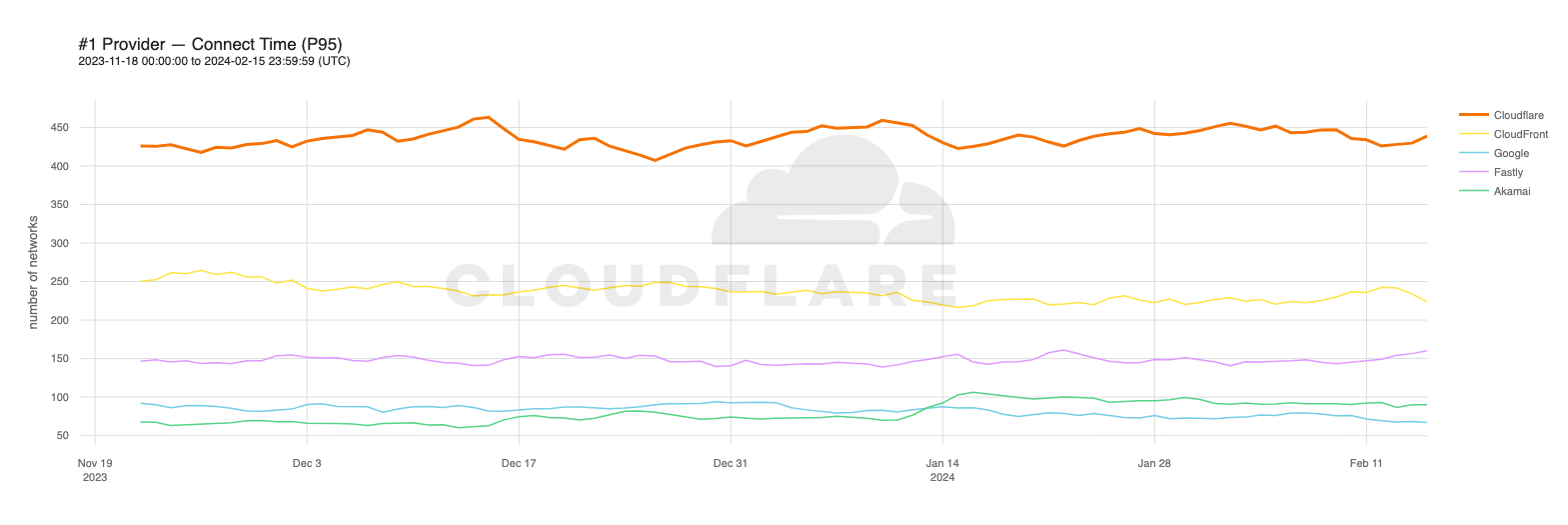
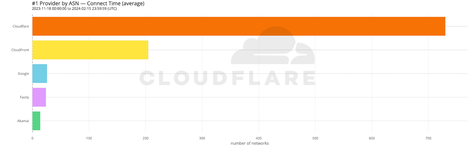
Looking at 95th percentile TCP connect times from November 18, 2023, to February 15, 2024, Cloudflare is the #1 provider in 44% of the top 1000 networks:
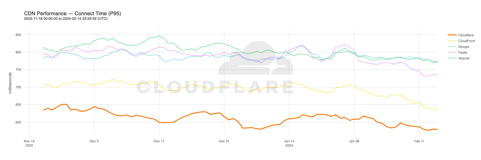
Our P95 TCP Connection time has been trending down since November, and we are consistently 50ms faster at P95 than our closest competitor (Amazon CloudFront):
Connect time comparisons between providers at 50th and 95th percentile
P50 Connect (ms)
P95 Connect (ms)
Cloudflare
130
579
Amazon
145
637
Google
190
772
Akamai
195
774
Fastly
189
734
These graphs show that day over day, Cloudflare was consistently the fastest provider. They also show the gaps between Cloudflare and the other competitors. When you look at the 95th percentile, Cloudflare is almost 200ms faster than Akamai across the world for connect times. This shows that our network reaches more places and allows users to get their content faster than Akamai on a consistent basis.
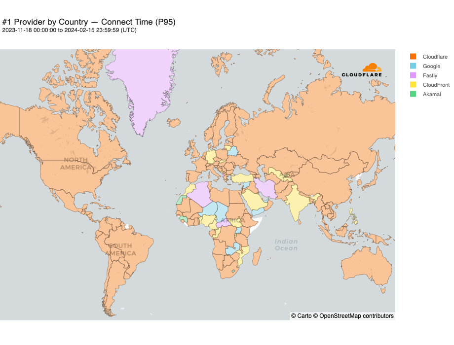
When we aggregate this data over the whole time period, Cloudflare is the fastest in the most networks. For that whole time span of November 18, 2023, to February 15, 2024, Cloudflare was number 1 in 73% of networks for mean TCP connection time:
Looking at a map plotting by 95th percentile TCP connect time, Cloudflare is the fastest in the most countries, and you can see this by the fact that most of the map is orange:
For comparison, here’s what the map looked like in September 2023:
These numbers show that we’re reducing the overall TCP connection time around the world while simultaneously staying ahead of the competition. Let’s talk about how we get these numbers and what we’re doing to make you even faster.
Measuring What Matters
As a quick reminder, here’s how we get the data for our measurements: when users receive a Cloudflare-branded error page, we use Real User Measurements (RUM) and fetch a small file from Cloudflare, Akamai, Amazon CloudFront, Fastly, and Google Cloud CDN. Browsers around the world report the performance of those providers from the perspective of the end-user network they are on. The goal is to provide an accurate picture of where different providers are faster, and more importantly, where Cloudflare can improve. You can read more about the methodology in the original Speed Week blog post.
Using the RUM data, we measure various performance metrics, such as TCP Connection Time, Time to First Byte (TTFB), and Time to Last Byte (TTLB), for ourselves and other providers.
If we only collect data from a browser when we return an error page, you could see how variable the data can get: if one network or website is having a problem in a certain country, that country could overreport, meaning those networks would be more highly weighted in the calculations because more users reported from that network during a given time period.
For example, if a lot of users connecting over a small Brazilian network were generating reports because their websites were throwing errors more frequently, that could make this small network look a lot bigger to us. This small network in Brazil could have as many reports as Claro, a major network in the region, despite them being totally different when you look at the number of subscribers. If we only look at the networks that report to us the most, it could cause smaller networks with fewer subscribers to be treated as more important because of point-in-time error conditions.
This phenomenon could cause the networks we look at to change week over week. Going back to the Brazil example, if the website that was throwing a bunch of errors fixed their problem, and we no longer saw measurements from that network, they may not show up as a “most reported network” depending on when we look at the data. This means that the networks we look at to consider where we are fastest are dependent on which networks are sending us the most reports at any given time, which is not optimal if we’re trying to get faster in these networks. We need to be able to get a consistent signal on these networks to understand where we’re faster and where we’re not.
We’ve addressed this issue by creating a fixed list of the networks we want to look at. We did this by looking at public stats on user population by network and then comparing that with our sample sizes by network until we identified the 1000 networks we want to examine. This ensures that day over day, the networks we look at are the same.
Now let’s talk about what makes us faster in more places than other networks: HTTP/3.
Blazing fast speeds with HTTP/3
One reason why Cloudflare is the fastest in the most networks is because we’ve been leading the charge with adoption and usage of HTTP/3 on our platform. HTTP/3 allows for faster connectivity behavior which means we can get connections established faster and get data flowing. HTTP/3 is currently used by around 31% of Internet traffic:
To show that HTTP/3 improves connection times, we looked at two different Cloudflare endpoints that these tests ran against: one with HTTP/3 enabled and one with HTTP/3 disabled. The performance difference between the two is night and day. Here’s a table showing the performance difference for 95th percentile connect time between Cloudflare zones when one zone has HTTP/3 enabled:
P50 connect (ms)
P95 connect (ms)
Cloudflare HTTP/3
130
579
Cloudflare non-HTTP/3
174
695
At P95, Cloudflare is 116 ms faster for connection times when HTTP/3 is enabled. This performance gain helps us be the fastest in the most networks.
But why does HTTP/3 help make us faster? HTTP/3 allows for faster connection setup times, which lets us take greater advantage of our global network footprint to be the fastest in the most networks. HTTP/3 is built on top of the QUIC protocol, which multiplexes UDP packets to allow for parallel streams to be sent at the same time. This means that TLS encryption can happen in parallel with connection establishment, shortening the amount of time that is needed to set up a secure connection. Paired with Cloudflare’s network that is incredibly close to end-users, this makes for significant latency reductions on user Connect times. All major browsers have HTTP/3 enabled by default, so you too can realize these latency improvements by enabling HTTP/3 on your website today.
What’s next
We’re sharing our updates on our journey to become #1 everywhere so that you can see what goes into running the fastest network in the world. From here, our plan is the same as always: identify where we’re slower, fix it, and then tell you how we’ve gotten faster.
A key component of effective corporate network security is establishing end to end visibility across all traffic that flows through the network. Every network engineer needs a complete overview of their network traffic to confirm their security policies work, to identify new vulnerabilities, and to analyze any shifts in traffic behavior. Often, it’s difficult to build out effective network monitoring as teams struggle with problems like configuring and tuning data collection, managing storage costs, and analyzing traffic across multiple visibility tools.
Today, we’re excited to announce that a free version of Cloudflare’s network flow monitoring product, Magic Network Monitoring, is available to all Enterprise Customers. Every Enterprise Customer can configure Magic Network Monitoring and immediately improve their network visibility in as little as 30 minutes via our self-serve onboarding process.
Enterprise Customers can visit the Magic Network Monitoring product page, click “Talk to an expert”, and fill out the form. You’ll receive access within 24 hours of submitting the request. Over the next month, the free version of Magic Network Monitoring will be rolled out to all Enterprise Customers. The product will automatically be available by default without the need to submit a form.
How it works
Cloudflare customers can send their network flow data (either NetFlow or sFlow) from their routers to Cloudflare’s network edge.
Magic Network Monitoring will pick up this data, parse it, and instantly provide insights and analytics on your network traffic. These analytics include traffic volume overtime in bytes and packets, top protocols, sources, destinations, ports, and TCP flags.
Dogfooding Magic Network Monitoring during the remediation of the Thanksgiving 2023 security incident
Let’s review a recent example of how Magic Network Monitoring improved Cloudflare’s own network security and traffic visibility during the Thanksgiving 2023 security incident. Our security team needed a lightweight method to identify malicious packet characteristics in our core data center traffic. We monitored for any network traffic sourced from or destined to a list of ASNs associated with the bad actor. Our security team setup Magic Network Monitoring and established visibility into our first core data center within 24 hours of the project kick-off. Today, Cloudflare continues to use Magic Network Monitoring to monitor for traffic related to bad actors and to provide real time traffic analytics on more than 1 Tbps of core data center traffic.
Magic Network Monitoring – Traffic Analytics
Monitoring local network traffic from IoT devices
Magic Network Monitoring also improves visibility on any network traffic that doesn’t go through Cloudflare. Imagine that you’re a network engineer at ACME Corporation, and it’s your job to manage and troubleshoot IoT devices in a factory that are connected to the factory’s internal network. The traffic generated by these IoT devices doesn’t go through Cloudflare because it is destined to other devices and endpoints on the internal network. Nonetheless, you still need to establish network visibility into device traffic over time to monitor and troubleshoot the system.
To solve the problem, you configure a router or other network device to securely send encrypted traffic flow summaries to Cloudflare via an IPSec tunnel. Magic Network Monitoring parses the data, and instantly provides you with insights and analytics on your network traffic. Now, when an IoT device goes down, or a connection between IoT devices is unexpectedly blocked, you can analyze historical network traffic data in Magic Network Monitoring to speed up the troubleshooting process.
Monitoring cloud network traffic
As cloud networking becomes increasingly prevalent, it is essential for enterprises to invest in visibility across their cloud environments. Let’s say you’re responsible for monitoring and troubleshooting your corporation’s cloud network operations which are spread across multiple public cloud providers. You need to improve visibility into your cloud network traffic to analyze and troubleshoot any unexpected traffic patterns like configuration drift that leads to an exposed network port.
To improve traffic visibility across different cloud environments, you can export cloud traffic flow logs from any virtual device that supports NetFlow or sFlow to Cloudflare. In the future, we are building support for native cloud VPC flow logs in conjunction with Magic Cloud Networking. Cloudflare will parse this traffic flow data and provide alerts plus analytics across all your cloud environments in a single pane of glass on the Cloudflare dashboard.
Improve your security posture today in less than 30 minutes
If you’re an existing Enterprise customer, and you want to improve your corporate network security, you can get started right away. Visit the Magic Network Monitoring product page, click “Talk to an expert”, and fill out the form. You’ll receive access within 24 hours of submitting the request. You can begin the self-serve onboarding tutorial, and start monitoring your first batch of network traffic in less than 30 minutes.
Over the next month, the free version of Magic Network Monitoring will be rolled out to all Enterprise Customers. The product will be automatically available by default without the need to submit a form.
If you’re interested in becoming an Enterprise Customer, and have more questions about Magic Network Monitoring, you can talk with an expert. If you’re a free customer, and you’re interested in testing a limited beta of Magic Network Monitoring, you can fill out this form to request access.
Today we are excited to announce Magic Cloud Networking, supercharged by Cloudflare’s recent acquisition of Nefeli Networks’ innovative technology. These new capabilities to visualize and automate cloud networks will give our customers secure, easy, and seamless connection to public cloud environments.
Public clouds offer organizations a scalable and on-demand IT infrastructure without the overhead and expense of running their own datacenter. Cloud networking is foundational to applications that have been migrated to the cloud, but is difficult to manage without automation software, especially when operating at scale across multiple cloud accounts. Magic Cloud Networking uses familiar concepts to provide a single interface that controls and unifies multiple cloud providers’ native network capabilities to create reliable, cost-effective, and secure cloud networks.
Nefeli’s approach to multi-cloud networking solves the problem of building and operating end-to-end networks within and across public clouds, allowing organizations to securely leverage applications spanning any combination of internal and external resources. Adding Nefeli’s technology will make it easier than ever for our customers to connect and protect their users, private networks and applications.
Why is cloud networking difficult?
Compared with a traditional on-premises data center network, cloud networking promises simplicity:
Much of the complexity of physical networking is abstracted away from users because the physical and ethernet layers are not part of the network service exposed by the cloud provider.
There are fewer control plane protocols; instead, the cloud providers deliver a simplified software-defined network (SDN) that is fully programmable via API.
There is capacity — from zero up to very large — available instantly and on-demand, only charging for what you use.
However, that promise has not yet been fully realized. Our customers have described several reasons cloud networking is difficult:
Poor end-to-end visibility: Cloud network visibility tools are difficult to use and silos exist even within single cloud providers that impede end-to-end monitoring and troubleshooting.
Faster pace: Traditional IT management approaches clash with the promise of the cloud: instant deployment available on-demand. Familiar ClickOps and CLI-driven procedures must be replaced by automation to meet the needs of the business.
Different technology: Established network architectures in on-premises environments do not seamlessly transition to a public cloud. The missing ethernet layer and advanced control plane protocols were critical in many network designs.
New cost models: The dynamic pay-as-you-go usage-based cost models of the public clouds are not compatible with established approaches built around fixed cost circuits and 5-year depreciation. Network solutions are often architected with financial constraints, and accordingly, different architectural approaches are sensible in the cloud.
New security risks: Securing public clouds with true zero trust and least-privilege demands mature operating processes and automation, and familiarity with cloud-specific policies and IAM controls.
Multi-vendor: Oftentimes enterprise networks have used single-vendor sourcing to facilitate interoperability, operational efficiency, and targeted hiring and training. Operating a network that extends beyond a single cloud, into other clouds or on-premises environments, is a multi-vendor scenario.
Nefeli considered all these problems and the tensions between different customer perspectives to identify where the problem should be solved.
Trains, planes, and automation
Consider a train system. To operate effectively it has three key layers:
tracks and trains
electronic signals
a company to manage the system and sell tickets.
A train system with good tracks, trains, and signals could still be operating below its full potential because its agents are unable to keep up with passenger demand. The result is that passengers cannot plan itineraries or purchase tickets.
The train company eliminates bottlenecks in process flow by simplifying the schedules, simplifying the pricing, providing agents with better booking systems, and installing automated ticket machines. Now the same fast and reliable infrastructure of tracks, trains, and signals can be used to its full potential.
Solve the right problem
In networking, there are an analogous set of three layers, called the networking planes:
Data Plane: the network paths that transport data (in the form of packets) from source to destination.
Control Plane: protocols and logic that change how packets are steered across the data plane.
Management Plane: the configuration and monitoring interfaces for the data plane and control plane.
In public cloud networks, these layers map to:
Cloud Data Plane: The underlying cables and devices are exposed to users as the Virtual Private Cloud (VPC) or Virtual Network (VNet) service that includes subnets, routing tables, security groups/ACLs and additional services such as load-balancers and VPN gateways.
Cloud Control Plane: In place of distributed protocols, the cloud control plane is a software defined network (SDN) that, for example, programs static route tables. (There is limited use of traditional control plane protocols, such as BGP to interface with external networks and ARP to interface with VMs.)
Cloud Management Plane: An administrative interface with a UI and API which allows the admin to fully configure the data and control planes. It also provides a variety of monitoring and logging capabilities that can be enabled and integrated with 3rd party systems.
Like our train example, most of the problems that our customers experience with cloud networking are in the third layer: the management plane.
Nefeli simplifies, unifies, and automates cloud network management and operations.
Avoid cost and complexity
One common approach to tackle management problems in cloud networks is introducing Virtual Network Functions (VNFs), which are virtual machines (VMs) that do packet forwarding, in place of native cloud data plane constructs. Some VNFs are routers, firewalls, or load-balancers ported from a traditional network vendor’s hardware appliances, while others are software-based proxies often built on open-source projects like NGINX or Envoy. Because VNFs mimic their physical counterparts, IT teams could continue using familiar management tooling, but VNFs have downsides:
VMs do not have custom network silicon and so instead rely on raw compute power. The VM is sized for the peak anticipated load and then typically runs 24x7x365. This drives a high cost of compute regardless of the actual utilization.
High-availability (HA) relies on fragile, costly, and complex network configuration.
Service insertion — the configuration to put a VNF into the packet flow — often forces packet paths that incur additional bandwidth charges.
VNFs are typically licensed similarly to their on-premises counterparts and are expensive.
VNFs lock in the enterprise and potentially exclude them benefitting from improvements in the cloud’s native data plane offerings.
For these reasons, enterprises are turning away from VNF-based solutions and increasingly looking to rely on the native network capabilities of their cloud service providers. The built-in public cloud networking is elastic, performant, robust, and priced on usage, with high-availability options integrated and backed by the cloud provider’s service level agreement.
In our train example, the tracks and trains are good. Likewise, the cloud network data plane is highly capable. Changing the data plane to solve management plane problems is the wrong approach. To make this work at scale, organizations need a solution that works together with the native network capabilities of cloud service providers.
Nefeli leverages native cloud data plane constructs rather than third party VNFs.
Introducing Magic Cloud Networking
The Nefeli team has joined Cloudflare to integrate cloud network management functionality with Cloudflare One. This capability is called Magic Cloud Networking and with it, enterprises can use the Cloudflare dashboard and API to manage their public cloud networks and connect with Cloudflare One.
End-to-end
Just as train providers are focused only on completing train journeys in their own network, cloud service providers deliver network connectivity and tools within a single cloud account. Many large enterprises have hundreds of cloud accounts across multiple cloud providers. In an end-to-end network this creates disconnected networking silos which introduce operational inefficiencies and risk.
Imagine you are trying to organize a train journey across Europe, and no single train company serves both your origin and destination. You know they all offer the same basic service: a seat on a train. However, your trip is difficult to arrange because it involves multiple trains operated by different companies with their own schedules and ticketing rates, all in different languages!
Magic Cloud Networking is like an online travel agent that aggregates multiple transportation options, books multiple tickets, facilitates changes after booking, and then delivers travel status updates.
Through the Cloudflare dashboard, you can discover all of your network resources across accounts and cloud providers and visualize your end-to-end network in a single interface. Once Magic Cloud Networking discovers your networks, you can build a scalable network through a fully automated and simple workflow.
Resource inventory shows all configuration in a single and responsive UI
Taming per-cloud complexity
Public clouds are used to deliver applications and services. Each cloud provider offers a composable stack of modular building blocks (resources) that start with the foundation of a billing account and then add on security controls. The next foundational layer, for server-based applications, is VPC networking. Additional resources are built on the VPC network foundation until you have compute, storage, and network infrastructure to host the enterprise application and data. Even relatively simple architectures can be composed of hundreds of resources.
The trouble is, these resources expose abstractions that are different from the building blocks you would use to build a service on prem, the abstractions differ between cloud providers, and they form a web of dependencies with complex rules about how configuration changes are made (rules which differ between resource types and cloud providers). For example, say I create 100 VMs, and connect them to an IP network. Can I make changes to the IP network while the VMs are using the network? The answer: it depends.
Magic Cloud Networking handles these differences and complexities for you. It configures native cloud constructs such as VPN gateways, routes, and security groups to securely connect your cloud VPC network to Cloudflare One without having to learn each cloud’s incantations for creating VPN connections and hubs.
Continuous, coordinated automation
Returning to our train system example, what if the railway maintenance staff find a dangerous fault on the railroad track? They manually set the signal to a stop light to prevent any oncoming trains using the faulty section of track. Then, what if, by unfortunate coincidence, the scheduling office is changing the signal schedule, and they set the signals remotely which clears the safety measure made by the maintenance crew? Now there is a problem that no one knows about and the root cause is that multiple authorities can change the signals via different interfaces without coordination.
The same problem exists in cloud networks: configuration changes are made by different teams using different automation and configuration interfaces across a spectrum of roles such as billing, support, security, networking, firewalls, database, and application development.
Once your network is deployed, Magic Cloud Networking monitors its configuration and health, enabling you to be confident that the security and connectivity you put in place yesterday is still in place today. It tracks the cloud resources it is responsible for, automatically reverting drift if they are changed out-of-band, while allowing you to manage other resources, like storage buckets and application servers, with other automation tools. And, as you change your network, Cloudflare takes care of route management, injecting and withdrawing routes globally across Cloudflare and all connected cloud provider networks.
Magic Cloud Networking is fully programmable via API, and can be integrated into existing automation toolchains.
The interface warns when cloud network infrastructure drifts from intent
Ready to start conquering cloud networking?
We are thrilled to introduce Magic Cloud Networking as another pivotal step to fulfilling the promise of the Connectivity Cloud. This marks our initial stride in empowering customers to seamlessly integrate Cloudflare with their public clouds to get securely connected, stay securely connected, and gain flexibility and cost savings as they go.
Join us on this journey for early access: learn more and sign up here.
It is no secret that Cloudflare is encouraging companies to deprecate their use of IPv4 addresses and move to IPv6 addresses. We have a couple articles on the subject from this year:
And many more in our catalog. To help with this, we spent time this last year investigating and implementing infrastructure to reduce our internal and egress use of IPv4 addresses. We prefer to re-allocate our addresses than to purchase more due to increasing costs. And in this effort we discovered that our cache service is one of our bigger consumers of IPv4 addresses. Before we remove IPv4 addresses for our cache services, we first need to understand how cache works at Cloudflare.
How does cache work at Cloudflare?
Describing the full scope of the architecture is out of scope of this article, however, we can provide a basic outline:
Internet User makes a request to pull an asset
Cloudflare infrastructure routes that request to a handler
Handler machine returns cached asset, or if miss
Handler machine reaches to origin server (owned by a customer) to pull the requested asset
The particularly interesting part is the cache miss case. When a very popular origin has an uncached asset that many Internet Users are trying to access at once, we may make upwards of: 50k TCP unicast connections to a single destination.
That is a lot of connections! We have strategies in place to limit the impact of this or avoid this problem altogether. But in these rare cases when it occurs, we will then balance these connections over two source IPv4 addresses.
Our goal is to remove the load balancing and prefer one IPv4 address. To do that, we need to understand the performance impact of two IPv4 addresses vs one.
TCP connect() performance of two source IPv4 addresses vs one IPv4 address
We leveraged a tool called wrk, and modified it to distribute connections over multiple source IP addresses. Then we ran a workload of 70k connections over 48 threads for a period of time.
During the test we measured the function tcp_v4_connect() with the BPF BCC libbpf-tool funclatency tool to gather latency metrics as time progresses.
Note that throughout the rest of this article, all the numbers are specific to a single machine with no production traffic. We are making the assumption that if we can improve a worse case scenario in an algorithm with a best case machine, that the results could be extrapolated to production. Lock contention was specifically taken out of the equation, but will have production implications.
Two IPv4 addresses
The y-axis are buckets of nanoseconds in powers of ten. The x-axis represents the number of connections made per bucket. Therefore, more connections in a lower power of ten buckets is better.
We can see that the majority of the connections occur in the fast case with roughly ~20k in the slow case. We should expect this bimodal to increase over time due to wrk continuously closing and establishing connections.
Now let us look at the performance of one IPv4 address under the same conditions.
One IPv4 address
In this case, the bimodal distribution is even more pronounced. Over half of the total connections are in the slow case than in the fast! We may conclude that simply switching to one IPv4 address for cache egress is going to introduce significant latency on our connect() syscalls.
The next logical step is to figure out where this bottleneck is happening.
Port selection is not what you think it is
To investigate this, we first took a flame graph of a production machine:
Flame graphs depict a run-time function call stack of a system. Y-axis depicts call-stack depth, and x-axis depicts a function name in a horizontal bar that represents the amount of times the function was sampled. Checkout this in-depth guide about flame graphs for more details.
Most of the samples are taken in the function __inet_hash_connect(). We can see that there are also many samples for __inet_check_established() with some lock contention sampled between. We have a better picture of a potential bottleneck, but we do not have a consistent test to compare against.
Wrk introduces a bit more variability than we would like to see. Still focusing on the function tcp_v4_connect(), we performed another synthetic test with a homegrown benchmark tool to test one IPv4 address. A tool such as stress-ng may also be used, but some modification is necessary to implement the socket option IP_LOCAL_PORT_RANGE. There is more about that socket option later.
We are now going to ensure a deterministic amount of connections, and remove lock contention from the problem. The result is something like this:
On the y-axis we measured the latency between the start and end of a connect() syscall. The x-axis denotes when a connect() was called. Green dots are even numbered ports, and red dots are odd numbered ports. The orange line is a linear-regression on the data.
The disparity between the average time for port allocation between even and odd ports provides us with a major clue. Connections with odd ports are found significantly slower than the even. Further, odd ports are not interleaved with earlier connections. This implies we exhaust our even ports before attempting the odd. The chart also confirms our bimodal distribution.
__inet_hash_connect()
At this point we wanted to understand this split a bit better. We know from the flame graph and the function __inet_hash_connect() that this holds the algorithm for port selection. For context, this function is responsible for associating the socket to a source port in a late bind. If a port was previously provided with bind(), the algorithm just tests for a unique TCP 4-tuple (src ip, src port, dest ip, dest port) and ignores port selection.
Before we dive in, there is a little bit of setup work that happens first. Linux first generates a time-based hash that is used as the basis for the starting port, then adds randomization, and then puts that information into an offset variable. This is always set to an even integer.
   offset &= ~1U;

other_parity_scan:
    port = low + offset;
    for (i = 0; i < remaining; i += 2, port += 2) {
        if (unlikely(port >= high))
            port -= remaining;

        inet_bind_bucket_for_each(tb, &head->chain) {
            if (inet_bind_bucket_match(tb, net, port, l3mdev)) {
                if (!check_established(death_row, sk, port, &tw))
                    goto ok;
                goto next_port;
            }
        }
    }

    offset++;
    if ((offset & 1) && remaining > 1)
        goto other_parity_scan;
Then in a nutshell: loop through one half of ports in our range (all even or all odd ports) before looping through the other half of ports (all odd or all even ports respectively) for each connection. Specifically, this is a variation of the Double-Hash Port Selection Algorithm. We will ignore the bind bucket functionality since that is not our main concern.
Depending on your port range, you either start with an even port or an odd port. In our case, our low port, 9024, is even. Then the port is picked by adding the offset to the low port:
If low was odd, we will have an odd starting port because odd + even = odd.
There is a bit too much going on in the loop to explain in text. I have an example instead:
This example is bound by 8 ports and 8 possible connections. All ports start unused. As a port is used up, the port is grayed out. Green boxes represent the next chosen port. All other colors represent open ports. Blue arrows are even port iterations of offset, and red are the odd port iterations of offset. Note that the offset is randomly picked, and once we cross over to the odd range, the offset is incremented by one.
For each selection of a port, the algorithm then makes a call to the function check_established() which dereferences __inet_check_established(). This function loops over sockets to verify that the TCP 4-tuple is unique. The takeaway is that the socket list in the function is usually smaller than not. This grows as more unique TCP 4-tuples are introduced to the system. Longer socket lists may slow down port selection eventually. We have a blog post that dives into the socket list and port uniqueness criteria.
At this point, we can summarize that the odd/even port split is what is causing our performance bottleneck. And during the investigation, it was not obvious to me (or even maybe you) why the offset was initially calculated the way it was, and why the odd/even port split was introduced. After some git-archaeology the decisions become more clear.
Security considerations
Port selection has been shown to be used in device fingerprinting in the past. This led the authors to introduce more randomization into the initial port selection. Prior, ports were predictably picked solely based on their initial hash and a salt value which does not change often. This helps with explaining the offset, but does not explain the split.
Why the even/odd split?
Prior to this patch and that patch, services may have conflicts between the connect() and bind() heavy workloads. Thus, to avoid those conflicts, the split was added. An even offset was chosen for the connect() workloads, and an odd offset for the bind() workloads. However, we can see that the split works great for connect() workloads that do not exceed one half of the allotted port range.
Now we have an explanation for the flame graph and charts. So what can we do about this?
User space solution (kernel < 6.8)
We have a couple of strategies that would work best for us. Infrastructure or architectural strategies are not considered due to significant development effort. Instead, we prefer to tackle the problem where it occurs.
Select, test, repeat
For the “select, test, repeat” approach, you may have code that ends up looking like this:
sys = get_ip_local_port_range()
estab = 0
i = sys.hi
while i >= 0:
    if estab >= sys.hi:
        break

    random_port = random.randint(sys.lo, sys.hi)
    connection = attempt_connect(random_port)
    if connection is None:
        i += 1
        continue

    i -= 1
    estab += 1
The algorithm simply loops through the system port range, and randomly picks a port each iteration. Then test that the connect() worked. If not, rinse and repeat until range exhaustion.
This approach is good for up to ~70-80% port range utilization. And this may take roughly eight to twelve attempts per connection as we approach exhaustion. The major downside to this approach is the extra syscall overhead on conflict. In order to reduce this overhead, we can consider another approach that allows the kernel to still select the port for us.
Select port by random shifting range
This approach leverages the IP_LOCAL_PORT_RANGE socket option. And we were able to achieve performance like this:
That is much better! The chart also introduces black dots that represent errored connections. However, they have a tendency to clump at the very end of our port range as we approach exhaustion. This is not dissimilar to what we may see in “select, test, repeat”.
We first fetch the system’s local port range, define a custom port range, and then randomly shift the custom range within the system range. Introducing this randomization helps the kernel to start port selection randomly at an odd or even port. Then reduces the loop search space down to the range of the custom window.
We tested with a few different window sizes, and determined that a five hundred or one thousand size works fairly well for our port range:
Window size
Errors
Total test time
Connections/second
500
868
~1.8 seconds
~30,139
1,000
1,129
~2 seconds
~27,260
5,000
4,037
~6.7 seconds
~8,405
10,000
6,695
~17.7 seconds
~3,183
As the window size increases, the error rate increases. That is because a larger window provides less random offset opportunity. A max window size of 56,512 is no different from using the kernels default behavior. Therefore, a smaller window size works better. But you do not want it to be too small either. A window size of one is no different from “select, test, repeat”.
In kernels >= 6.8, we can do even better.
Kernel solution (kernel >= 6.8)
A new patch was introduced that eliminates the need for the window shifting. This solution is going to be available in the 6.8 kernel.
Instead of picking a random window offset for setsockopt(IPPROTO_IP, IP_LOCAL_PORT_RANGE, …), like in the previous solution, we instead just pass the full system port range to activate the solution. The code may look something like this:
Setting IP_LOCAL_PORT_RANGE option is what tells the kernel to use a similar approach to “select port by random shifting range” such that the start offset is randomized to be even or odd, but then loops incrementally rather than skipping every other port. We end up with results like this:
The performance of this approach is quite comparable to our user space implementation. Albeit, a little faster. Due in part to general improvements, and that the algorithm can always find a port given the full search space of the range. Then there are no cycles wasted on a potentially filled sub-range.
These results are great for TCP, but what about other protocols?
Other protocols & connect()
It is worth mentioning at this point that the algorithms used for the protocols are mostly the same for IPv4 & IPv6. Typically, the key difference is how the sockets are compared to determine uniqueness and where the port search happens. We did not compare performance for all protocols. But it is worth mentioning some similarities and differences with TCP and a couple of others.
DCCP
The DCCP protocol leverages the same port selection algorithm as TCP. Therefore, this protocol benefits from the recent kernel changes. It is also possible the protocol could benefit from our user space solution, but that is untested. We will let the reader exercise DCCP use-cases.
UDP & UDP-Lite
UDP leverages a different algorithm found in the function udp_lib_get_port(). Similar to TCP, the algorithm will loop over the whole port range space incrementally. This is only the case if the port is not already supplied in the bind() call. The key difference between UDP and TCP is that a random number is generated as a step variable. Then, once a first port is identified, the algorithm loops on that port with the random number. This relies on an uint16_t overflow to eventually loop back to the chosen port. If all ports are used, increment the port by one and repeat. There is no port splitting between even and odd ports.
The best comparison to the TCP measurements is a UDP setup similar to:
sk = socket(AF_INET, SOCK_DGRAM)
sk.bind((src_ip, 0))
sk.connect((dest_ip, dest_port))
And the results should be unsurprising with one IPv4 source address:
UDP fundamentally behaves differently from TCP. And there is less work overall for port lookups. The outliers in the chart represent a worst-case scenario when we reach a fairly bad random number collision. In that case, we need to more-completely loop over the ephemeral range to find a port.
UDP has another problem. Given the socket option SO_REUSEADDR, the port you get back may conflict with another UDP socket. This is in part due to the function udp_lib_lport_inuse() ignoring the UDP 2-tuple (src ip, src port) check given the socket option. When this happens you may have a new socket that overwrites a previous. Extra care is needed in that case. We wrote more in depth about these cases in a previous blog post.
In summary
Cloudflare can make a lot of unicast egress connections to origin servers with popular uncached assets. To avoid port-resource exhaustion, we balance the load over a couple of IPv4 source addresses during those peak times. Then we asked: “what is the performance impact of one IPv4 source address for our connect()-heavy workloads?”. Port selection is not only difficult to get right, but is also a performance bottleneck. This is evidenced by measuring connect() latency with a flame graph and synthetic workloads. That then led us to discovering TCP’s quirky port selection process that loops over half your ephemeral ports before the other for each connect().
We then proposed three solutions to solve the problem outside of adding more IP addresses or other architectural changes: “select, test, repeat”, “select port by random shifting range”, and an IP_LOCAL_PORT_RANGE socket option solution in newer kernels. And finally closed out with other protocol honorable mentions and their quirks.
Do not take our numbers! Please explore and measure your own systems. With a better understanding of your workloads, you can make a good decision on which strategy works best for your needs. Even better if you come up with your own strategy!
Picture this: you’re at an airport, and you’re going through an airport security checkpoint. There are a bunch of agents who are scanning your boarding pass and your passport and sending you through to your gate. All of a sudden, some of the agents go on break. Maybe there’s a leak in the ceiling above the checkpoint. Or perhaps a bunch of flights are leaving at 6pm, and a number of passengers turn up at once. Either way, this imbalance between localized supply and demand can cause huge lines and unhappy travelers — who just want to get through the line to get on their flight. How do airports handle this?
Some airports may not do anything and just let you suffer in a longer line. Some airports may offer fast-lanes through the checkpoints for a fee. But most airports will tell you to go to another security checkpoint a little farther away to ensure that you can get through to your gate as fast as possible. They may even have signs up telling you how long each line is, so you can make an easier decision when trying to get through.
At Cloudflare, we have the same problem. We are located in 300 cities around the world that are built to receive end-user traffic for all of our product suites. And in an ideal world, we always have enough computers and bandwidth to handle everyone at their closest possible location. But the world is not always ideal; sometimes we take a data center offline for maintenance, or a connection to a data center goes down, or some equipment fails, and so on. When that happens, we may not have enough attendants to serve every person going through security in every location. It’s not because we haven’t built enough kiosks, but something has happened in our data center that prevents us from serving everyone.
So, we built Traffic Manager: a tool that balances supply and demand across our entire global network. This blog is about Traffic Manager: how it came to be, how we built it, and what it does now.
The world before Traffic Manager
The job now done by Traffic Manager used to be a manual process carried out by network engineers: our network would operate as normal until something happened that caused user traffic to be impacted at a particular data center.
When such events happened, user requests would start to fail with 499 or 500 errors because there weren’t enough machines to handle the request load of our users. This would trigger a page to our network engineers, who would then remove some Anycast routes for that data center. The end result: by no longer advertising those prefixes in the impacted data center, user traffic would divert to a different data center. This is how Anycast fundamentally works: user traffic is drawn to the closest data center advertising the prefix the user is trying to connect to, as determined by Border Gateway Protocol. For a primer on what Anycast is, check out this reference article.
Depending on how bad the problem was, engineers would remove some or even all the routes in a data center. When the data center was again able to absorb all the traffic, the engineers would put the routes back and the traffic would return naturally to the data center.
As you might guess, this was a challenging task for our network engineers to do every single time any piece of hardware on our network had an issue. It didn’t scale.
Never send a human to do a machine’s job
But doing it manually wasn’t just a burden on our Network Operations team. It also resulted in a sub-par experience for our customers; our engineers would need to take time to diagnose and re-route traffic. To solve both these problems, we wanted to build a service that would immediately and automatically detect if users were unable to reach a Cloudflare data center, and withdraw routes from the data center until users were no longer seeing issues. Once the service received notifications that the impacted data center could absorb the traffic, it could put the routes back and reconnect that data center. This service is called Traffic Manager, because its job (as you might guess) is to manage traffic coming into the Cloudflare network.
Accounting for second order consequences
When a network engineer removes a route from a router, they can make the best guess at where the user requests will move to, and try to ensure that the failover data center has enough resources to handle the requests — if it doesn’t, they can adjust the routes there accordingly prior to removing the route in the initial data center. To be able to automate this process, we needed to move from a world of intuition to a world of data — accurately predicting where traffic would go when a route was removed, and feeding this information to Traffic Manager, so it could ensure it doesn’t make the situation worse.
Meet Traffic Predictor
Although we can adjust which data centers advertise a route, we are unable to influence what proportion of traffic each data center receives. Each time we add a new data center, or a new peering session, the distribution of traffic changes, and as we are in over 300 cities and 12,500 peering sessions, it has become quite difficult for a human to keep track of, or predict the way traffic will move around our network. Traffic manager needed a buddy: Traffic Predictor.
In order to do its job, Traffic Predictor carries out an ongoing series of real world tests to see where traffic actually moves. Traffic Predictor relies on a testing system that simulates removing a data center from service and measuring where traffic would go if that data center wasn’t serving traffic. To help understand how this system works, let’s simulate the removal of a subset of a data center in Christchurch, New Zealand:
First, Traffic Predictor gets a list of all the IP addresses that normally connect to Christchurch. Traffic Predictor will send a ping request to hundreds of thousands of IPs that have recently made a request there.
Traffic Predictor records if the IP responds, and whether the response returns to Christchurch using a special Anycast IP range specifically configured for Traffic Predictor.
Once Traffic Predictor has a list of IPs that respond to Christchurch, it removes that route containing that special range from Christchurch, waits a few minutes for the Internet routing table to be updated, and runs the test again.
Instead of being routed to Christchurch, the responses are instead going to data centers around Christchurch. Traffic Predictor then uses the knowledge of responses for each data center, and records the results as the failover for Christchurch.
This allows us to simulate Christchurch going offline without actually taking Christchurch offline!
But Traffic Predictor doesn’t just do this for any one data center. To add additional layers of resiliency, Traffic Predictor even calculates a second layer of indirection: for each data center failure scenario, Traffic Predictor also calculates failure scenarios and creates policies for when surrounding data centers fail.
Using our example from before, when Traffic Predictor tests Christchurch, it will run a series of tests that remove several surrounding data centers from service including Christchurch to calculate different failure scenarios. This ensures that even if something catastrophic happens which impacts multiple data centers in a region, we still have the ability to serve user traffic. If you think this data model is complicated, you’re right: it takes several days to calculate all of these failure paths and policies.
Here’s what those failure paths and failover scenarios look like for all of our data centers around the world when they’re visualized:
This can be a bit complicated for humans to parse, so let’s dig into that above scenario for Christchurch, New Zealand to make this a bit more clear. When we take a look at failover paths specifically for Christchurch, we see they look like this:
In this scenario we predict that 99.8% of Christchurch’s traffic would shift to Auckland, which is able to absorb all Christchurch traffic in the event of a catastrophic outage.
Traffic Predictor allows us to not only see where traffic will move to if something should happen, but it allows us to preconfigure Traffic Manager policies to move requests out of failover data centers to prevent a thundering herd scenario: where sudden influx of requests can cause failures in a second data center if the first one has issues. With Traffic Predictor, Traffic Manager doesn’t just move traffic out of one data center when that one fails, but it also proactively moves traffic out of other data centers to ensure a seamless continuation of service.
From a sledgehammer to a scalpel
With Traffic Predictor, Traffic Manager can dynamically advertise and withdraw prefixes while ensuring that every datacenter can handle all the traffic. But withdrawing prefixes as a means of traffic management can be a bit heavy-handed at times. One of the reasons for this is that the only way we had to add or remove traffic to a data center was through advertising routes from our Internet-facing routers. Each one of our routes has thousands of IP addresses, so removing only one still represents a large portion of traffic.
Specifically, Internet applications will advertise prefixes to the Internet from a /24 subnet at an absolute minimum, but many will advertise prefixes larger than that. This is generally done to prevent things like route leaks or route hijacks: many providers will actually filter out routes that are more specific than a /24 (for more information on that, check out this blog here). If we assume that Cloudflare maps protected properties to IP addresses at a 1:1 ratio, then each /24 subnet would be able to service 256 customers, which is the number of IP addresses in a /24 subnet. If every IP address sent one request per second, we’d have to move 4 /24 subnets out of a data center if we needed to move 1,000 requests per second (RPS).
But in reality, Cloudflare maps a single IP address to hundreds of thousands of protected properties. So for Cloudflare, a /24 might take 3,000 requests per second, but if we needed to move 1,000 RPS out, we would have no choice but to move a single /24 out. And that’s just assuming we advertise at a /24 level. If we used /20s to advertise, the amount we can withdraw gets less granular: at a 1:1 website to IP address mapping, that’s 4,096 requests per second for each prefix, and even more if the website to IP address mapping is many to one.
While withdrawing prefix advertisements improved the customer experience for those users who would have seen a 499 or 500 error — there may have been a significant portion of users who wouldn’t have been impacted by an issue who still were moved away from the data center they should have gone to, probably slowing them down, even if only a little bit. This concept of moving more traffic out than is necessary is called “stranding capacity”: the data center is theoretically able to service more users in a region but cannot because of how Traffic Manager was built.
We wanted to improve Traffic Manager so that it only moved the absolute minimum of users out of a data center that was seeing a problem and not strand any more capacity. To do so, we needed to shift percentages of prefixes, so we could be extra fine-grained and only move the things that absolutely need to be moved. To solve this, we built an extension of our Layer 4 load balancer Unimog, which we call Plurimog.
A quick refresher on Unimog and layer 4 load balancing: every single one of our machines contains a service that determines whether that machine can take a user request. If the machine can take a user request then it sends the request to our HTTP stack which processes the request before returning it to the user. If the machine can’t take the request, the machine sends the request to another machine in the data center that can. The machines can do this because they are constantly talking to each other to understand whether they can serve requests for users.
Plurimog does the same thing, but instead of talking between machines, Plurimog talks in between data centers and points of presence. If a request goes into Philadelphia and Philadelphia is unable to take the request, Plurimog will forward to another data center that can take the request, like Ashburn, where the request is decrypted and processed. Because Plurimog operates at layer 4, it can send individual TCP or UDP requests to other places which allows it to be very fine-grained: it can send percentages of traffic to other data centers very easily, meaning that we only need to send away enough traffic to ensure that everyone can be served as fast as possible. Check out how that works in our Frankfurt data center, as we are able to shift progressively more and more traffic away to handle issues in our data centers. This chart shows the number of actions taken on free traffic that cause it to be sent out of Frankfurt over time:
But even within a data center, we can route traffic around to prevent traffic from leaving the datacenter at all. Our large data centers, called Multi-Colo Points of Presence (MCPs) contain logical sections of compute within a data center that are distinct from one another. These MCP data centers are enabled with another version of Unimog called Duomog, which allows for traffic to be shifted between logical sections of compute automatically. This makes MCP data centers fault-tolerant without sacrificing performance for our customers, and allows Traffic Manager to work within a data center as well as between data centers.
When evaluating portions of requests to move, Traffic Manager does the following:
Traffic Manager identifies the proportion of requests that need to be removed from a data center or subsection of a data center so that all requests can be served.
Traffic Manager then calculates the aggregated space metrics for each target to see how many requests each failover data center can take.
Traffic Manager then identifies how much traffic in each plan we need to move, and moves either a proportion of the plan, or all of the plan through Plurimog/Duomog, until we've moved enough traffic. We move Free customers first, and if there are no more Free customers in a data center, we'll move Pro, and then Business customers if needed.
For example, let’s look at Ashburn, Virginia: one of our MCPs. Ashburn has nine different subsections of capacity that can each take traffic. On 8/28, one of those subsections, IAD02, had an issue that reduced the amount of traffic it could handle.
During this time period, Duomog sent more traffic from IAD02 to other subsections within Ashburn, ensuring that Ashburn was always online, and that performance was not impacted during this issue. Then, once IAD02 was able to take traffic again, Duomog shifted traffic back automatically. You can see these actions visualized in the time series graph below, which tracks the percentage of traffic moved over time between subsections of capacity within IAD02 (shown in green):
How does Traffic Manager know how much to move?
Although we used requests per second in the example above, using requests per second as a metric isn’t accurate enough when actually moving traffic. The reason for this is that different customers have different resource costs to our service; a website served mainly from cache with the WAF deactivated is much cheaper CPU wise than a site with all WAF rules enabled and caching disabled. So we record the time that each request takes in the CPU. We can then aggregate the CPU time across each plan to find the CPU time usage per plan. We record the CPU time in ms, and take a per second value, resulting in a unit of milliseconds per second.
CPU time is an important metric because of the impact it can have on latency and customer performance. As an example, consider the time it takes for an eyeball request to make it entirely through the Cloudflare front line servers: we call this the cfcheck latency. If this number goes too high, then our customers will start to notice, and they will have a bad experience. When cfcheck latency gets high, it’s usually because CPU utilization is high. The graph below shows 95th percentile cfcheck latency plotted against CPU utilization across all the machines in the same data center, and you can see the strong correlation:
So having Traffic Manager look at CPU time in a data center is a very good way to ensure that we’re giving customers the best experience and not causing problems.
After getting the CPU time per plan, we need to figure out how much of that CPU time to move to other data centers. To do this, we aggregate the CPU utilization across all servers to give a single CPU utilization across the data center. If a proportion of servers in the data center fail, due to network device failure, power failure, etc., then the requests that were hitting those servers are automatically routed elsewhere within the data center by Duomog. As the number of servers decrease, the overall CPU utilization of the data center increases. Traffic Manager has three thresholds for each data center; the maximum threshold, the target threshold, and the acceptable threshold:
Maximum: the CPU level at which performance starts to degrade, where Traffic Manager will take action
Target: the level to which Traffic Manager will try to reduce the CPU utilization to restore optimal service to users
Acceptable: the level below which a data center can receive requests forwarded from another data center, or revert active moves
When a data center goes above the maximum threshold, Traffic Manager takes the ratio of total CPU time across all plans to current CPU utilization, then applies that to the target CPU utilization to find the target CPU time. Doing it this way means we can compare a data center with 100 servers to a data center with 10 servers, without having to worry about the number of servers in each data center. This assumes that load increases linearly, which is close enough to true for the assumption to be valid for our purposes.
Target ratio equals current ratio:
Therefore:
Subtracting the target CPU time from the current CPU time gives us the CPU time to move:
For example, if the current CPU utilization was at 90% across the data center, the target was 85%, and the CPU time across all plans was 18,000, we would have:
This would mean Traffic Manager would need to move 1,000 CPU time:
Now we know the total CPU time needed to move, we can go through the plans, until the required time to move has been met.
What is the maximum threshold?
A frequent problem that we faced was determining at which point Traffic Manager should start taking action in a data center – what metric should it watch, and what is an acceptable level?
As said before, different services have different requirements in terms of CPU utilization, and there are many cases of data centers that have very different utilization patterns.
To solve this problem, we turned to machine learning. We created a service that will automatically adjust the maximum thresholds for each data center according to customer-facing indicators. For our main service-level indicator (SLI), we decided to use the cfcheck latency metric we described earlier.
But we also need to define a service-level objective (SLO) in order for our machine learning application to be able to adjust the threshold. We set the SLO for 20ms. Comparing our SLO to our SLI, our 95th percentile cfcheck latency should never go above 20ms and if it does, we need to do something. The below graph shows 95th percentile cfcheck latency over time, and customers start to get unhappy when cfcheck latency goes into the red zone:
If customers have a bad experience when CPU gets too high, then the goal of Traffic Manager’s maximum thresholds are to ensure that customer performance isn’t impacted and to start redirecting traffic away before performance starts to degrade. At a scheduled interval the Traffic Manager service will fetch a number of metrics for each data center and apply a series of machine learning algorithms. After cleaning the data for outliers we apply a simple quadratic curve fit, and we are currently testing a linear regression algorithm.
After fitting the models we can use them to predict the CPU usage when the SLI is equal to our SLO, and then use it as our maximum threshold. If we plot the cpu values against the SLI we can see clearly why these methods work so well for our data centers, as you can see for Barcelona in the graphs below, which are plotted against curve fit and linear regression fit respectively.
In these charts the vertical line is the SLO, and the intersection of this line with the fitted model represents the value that will be used as the maximum threshold. This model has proved to be very accurate, and we are able to significantly reduce the SLO breaches. Let’s take a look at when we started deploying this service in Lisbon:
Before the change, cfcheck latency was constantly spiking, but Traffic Manager wasn’t taking actions because the maximum threshold was static. But after July 29, we see that cfcheck latency has never hit the SLO because we are constantly measuring to make sure that customers are never impacted by CPU increases.
Where to send the traffic?
So now that we have a maximum threshold, we need to find the third CPU utilization threshold which isn’t used when calculating how much traffic to move – the acceptable threshold. When a data center is below this threshold, it has unused capacity which, as long as it isn’t forwarding traffic itself, is made available for other data centers to use when required. To work out how much each data center is able to receive, we use the same methodology as above, substituting target for acceptable:
Therefore:
Subtracting the current CPU time from the acceptable CPU time gives us the amount of CPU time that a data center could accept:
To find where to send traffic, Traffic Manager will find the available CPU time in all data centers, then it will order them by latency from the data center needing to move traffic. It moves through each of the data centers, using all available capacity based on the maximum thresholds before moving onto the next. When finding which plans to move, we move from the lowest priority plan to highest, but when finding where to send them, we move in the opposite direction.
To make this clearer let's use an example:
We need to move 1,000 CPU time from data center A, and we have the following usage per plan: Free: 500ms/s, Pro: 400ms/s, Business: 200ms/s, Enterprise: 1000ms/s.
We would move 100% of Free (500ms/s), 100% of Pro (400ms/s), 50% of Business (100ms/s), and 0% of Enterprise.
Nearby data centers have the following available CPU time: B: 300ms/s, C: 300ms/s, D: 1,000ms/s.
With latencies: A-B: 100ms, A-C: 110ms, A-D: 120ms.
Starting with the lowest latency and highest priority plan that requires action, we would be able to move all the Business CPU time to data center B and half of Pro. Next we would move onto data center C, and be able to move the rest of Pro, and 20% of Free. The rest of Free could then be forwarded to data center D. Resulting in the following action: Business: 50% → B, Pro: 50% → B, 50% → C, Free: 20% → C, 80% → D.
Reverting actions
In the same way that Traffic Manager is constantly looking to keep data centers from going above the threshold, it is also looking to bring any forwarded traffic back into a data center that is actively forwarding traffic.
Above we saw how Traffic Manager works out how much traffic a data center is able to receive from another data center — it calls this the available CPU time. When there is an active move we use this available CPU time to bring back traffic to the data center — we always prioritize reverting an active move over accepting traffic from another data center.
When you put this all together, you get a system that is constantly measuring system and customer health metrics for every data center and spreading traffic around to make sure that each request can be served given the current state of our network. When we put all of these moves between data centers on a map, it looks something like this, a map of all Traffic Manager moves for a period of one hour. This map doesn’t show our full data center deployment, but it does show the data centers that are sending or receiving moved traffic during this period:
Data centers in red or yellow are under load and shifting traffic to other data centers until they become green, which means that all metrics are showing as healthy. The size of the circles represent how many requests are shifted from or to those data centers. Where the traffic is going is denoted by where the lines are moving. This is difficult to see at a world scale, so let’s zoom into the United States to see this in action for the same time period:
Here you can see Toronto, Detroit, New York, and Kansas City are unable to serve some requests due to hardware issues, so they will send those requests to Dallas, Chicago, and Ashburn until equilibrium is restored for users and data centers. Once data centers like Detroit are able to service all the requests they are receiving without needing to send traffic away, Detroit will gradually stop forwarding requests to Chicago until any issues in the data center are completely resolved, at which point it will no longer be forwarding anything. Throughout all of this, end users are online and are not impacted by any physical issues that may be happening in Detroit or any of the other locations sending traffic.
Happy network, happy products
Because Traffic Manager is plugged into the user experience, it is a fundamental component of the Cloudflare network: it keeps our products online and ensures that they’re as fast and reliable as they can be. It’s our real time load balancer, helping to keep our products fast by only shifting necessary traffic away from data centers that are having issues. Because less traffic gets moved, our products and services stay fast.
But Traffic Manager can also help keep our products online and reliable because they allow our products to predict where reliability issues may occur and preemptively move the products elsewhere. For example, Browser Isolation directly works with Traffic Manager to help ensure the uptime of the product. When you connect to a Cloudflare data center to create a hosted browser instance, Browser Isolation first asks Traffic Manager if the data center has enough capacity to run the instance locally, and if so, the instance is created right then and there. If there isn’t sufficient capacity available, Traffic Manager tells Browser Isolation which the closest data center with sufficient available capacity is, thereby helping Browser Isolation to provide the best possible experience for the user.
Happy network, happy users
At Cloudflare, we operate this huge network to service all of our different products and customer scenarios. We’ve built this network for resiliency: in addition to our MCP locations designed to reduce impact from a single failure, we are constantly shifting traffic around on our network in response to internal and external issues.
But that is our problem — not yours.
Similarly, when human beings had to fix those issues, it was customers and end users who would be impacted. To ensure that you’re always online, we’ve built a smart system that detects our hardware failures and preemptively balances traffic across our network to ensure it’s online and as fast as possible. This system works faster than any person — not only allowing our network engineers to sleep at night — but also providing a better, faster experience for all of our customers.
And finally: if these kinds of engineering challenges sound exciting to you, then please consider checking out the Traffic Engineering team's open position on Cloudflare’s Careers page!
Almost three years ago, we launched Cloudflare Waiting Room to protect our customers’ sites from overwhelming spikes in legitimate traffic that could bring down their sites. Waiting Room gives customers control over user experience even in times of high traffic by placing excess traffic in a customizable, on-brand waiting room, dynamically admitting users as spots become available on their sites. Since the launch of Waiting Room, we’ve continued to expand its functionality based on customer feedback with features like mobile app support, analytics, Waiting Room bypass rules, and more.
We love announcing new features and solving problems for our customers by expanding the capabilities of Waiting Room. But, today, we want to give you a behind the scenes look at how we have evolved the core mechanism of our product–namely, exactly how it kicks in to queue traffic in response to spikes.
How was the Waiting Room built, and what are the challenges?
The diagram below shows a quick overview of where the Waiting room sits when a customer enables it for their website.
Waiting Room is built on Workers that runs across a global network of Cloudflare data centers. The requests to a customer’s website can go to many different Cloudflare data centers. To optimize for minimal latency and enhanced performance, these requests are routed to the data center with the most geographical proximity. When a new user makes a request to the host/path covered by the Waiting room, the waiting room worker decides whether to send the user to the origin or the waiting room. This decision is made by making use of the waiting room state which gives an idea of how many users are on the origin.
The waiting room state changes continuously based on the traffic around the world. This information can be stored in a central location or changes can get propagated around the world eventually. Storing this information in a central location can add significant latency to each request as the central location can be really far from where the request is originating from. So every data center works with its own waiting room state which is a snapshot of the traffic pattern for the website around the world available at that point in time. Before letting a user into the website, we do not want to wait for information from everywhere else in the world as that adds significant latency to the request. This is the reason why we chose not to have a central location but have a pipeline where changes in traffic get propagated eventually around the world.
This pipeline which aggregates the waiting room state in the background is built on Cloudflare Durable Objects. In 2021, we wrote a blog talking about how the aggregation pipeline works and the different design decisions we took there if you are interested. This pipeline ensures that every data center gets updated information about changes in traffic within a few seconds.
The Waiting room has to make a decision whether to send users to the website or queue them based on the state that it currently sees. This has to be done while making sure we queue at the right time so that the customer's website does not get overloaded. We also have to make sure we do not queue too early as we might be queueing for a falsely suspected spike in traffic. Being in a queue could cause some users to abandon going to the website. Waiting Room runs on every server in Cloudflare’s network, which spans over 300 cities in more than 100 countries. We want to make sure, for every new user, the decision whether to go to the website or the queue is made with minimal latency.This is what makes the decision of when to queue a hard question for the waiting room. In this blog, we will cover how we approached that tradeoff. Our algorithm has evolved to decrease the false positives while continuing to respect the customer’s set limits.
How a waiting room decides when to queue users
The most important factor that determines when your waiting room will start queuing is how you configured the traffic settings. There are two traffic limits that you will set when configuring a waiting room–total active users and new users per minute.The total active users is a target threshold for how many simultaneous users you want to allow on the pages covered by your waiting room. New users per minute defines the target threshold for the maximum rate of user influx to your website per minute. A sharp spike in either of these values might result in queuing. Another configuration that affects how we calculate the total active users is session duration. A user is considered active for session duration minutes since the request is made to any page covered by a waiting room.
The graph below is from one of our internal monitoring tools for a customer and shows a customer's traffic pattern for 2 days. This customer has set their limits, new users per minute and total active users to 200 and 200 respectively.
If you look at their traffic you can see that users were queued on September 11th around 11:45. At that point in time, the total active users was around 200. As the total active users ramped down (around 12:30), the queued users progressed to 0. The queueing started again on September 11th around 15:00 when total active users got to 200. The users that were queued around this time ensured that the traffic going to the website is around the limits set by the customer.
Once a user gets access to the website, we give them an encrypted cookie which indicates they have already gained access. The contents of the cookie can look like this.
The cookie is like a ticket which indicates entry to the waiting room.The bucketId indicates which cluster of users this user is part of. The acceptedAt time and lastCheckInTime indicate when the last interaction with the workers was. This information can ensure if the ticket is valid for entry or not when we compare it with the session duration value that the customer sets while configuring the waiting room. If the cookie is valid, we let the user through which ensures users who are on the website continue to be able to browse the website. If the cookie is invalid, we create a new cookie treating the user as a new user and if there is queueing happening on the website they get to the back of the queue. In the next section let us see how we decide when to queue those users.
To understand this further, let's see what the contents of the waiting room state are. For the customer we discussed above, at the time "Mon, 11 Sep 2023 11:45:54 GMT", the state could look like this.
{
  "activeUsers": 50,
}
As mentioned above the customer’s configuration has new users per minute and total active users equal to 200 and 200 respectively.
So the state indicates that there is space for the new users as there are only 50 active users when it's possible to have 200. So there is space for another 150 users to go in. Let's assume those 50 users could have come from two data centers San Jose (20 users) and London (30 users). We also keep track of the number of workers that are active across the globe as well as the number of workers active at the data center in which the state is calculated. The state key below could be the one calculated at San Jose.
Imagine at the time "Mon, 11 Sep 2023 11:45:54 GMT", we get a request to that waiting room at a datacenter in San Jose.
To see if the user that reached San Jose can go to the origin we first check the traffic history in the past minute to see the distribution of traffic at that time. This is because a lot of websites are popular in certain parts of the world. For a lot of these websites the traffic tends to come from the same data centers.
Looking at the traffic history for the minute "Mon, 11 Sep 2023 11:44:00 GMT" we see San Jose has 20 users out of 200 users going there (10%) at that time. For the current time "Mon, 11 Sep 2023 11:45:54 GMT" we divide the slots available at the website at the same ratio as the traffic history in the past minute. So we can send 10% of 150 slots available from San Jose which is 15 users. We also know that there are three active workers as "dataCenterWorkersActive" is 3.
The number of slots available for the data center is divided evenly among the workers in the data center. So every worker in San Jose can send 15/3 users to the website. If the worker that received the traffic has not sent any users to the origin for the current minute they can send up to five users (15/3).
At the same time ("Mon, 11 Sep 2023 11:45:54 GMT"), imagine a request goes to a data center in Delhi. The worker at the data center in Delhi checks the trafficHistory and sees that there are no slots allotted for it. For traffic like this we have reserved the Anywhere slots as we are really far away from the limit.
The Anywhere slots are divided among all the active workers in the globe as any worker around the world can take a part of this pie. 75% of the remaining 150 slots which is 113.
The state key also keeps track of the number of workers (globalWorkersActive) that have spawned around the world. The Anywhere slots allotted are divided among all the active workers in the world if available. globalWorkersActive is 10 when we look at the waiting room state. So every active worker can send as many as 113/10 which is approximately 11 users. So the first 11 users that come to a worker in the minute Mon, 11 Sep 2023 11:45:00 GMT gets admitted to the origin. The extra users get queued. The extra reserved slots (5) in San Jose for minute Mon, 11 Sep 2023 11:45:00 GMT discussed before ensures that we can admit up to 16(5 + 11) users from a worker from San Jose to the website.
Queuing at the worker level can cause users to get queued before the slots available for the data center
As we can see from the example above, we decide whether to queue or not at the worker level. The number of new users that go to workers around the world can be non-uniform. To understand what can happen when there is non-uniform distribution of traffic to two workers, let us look at the diagram below.
Imagine the slots available for a data center in San Jose are ten. There are two workers running in San Jose. Seven users go to worker1 and one user goes to worker2. In this situation worker1 will let in five out of the seven workers to the website and two of them get queued as worker1 only has five slots available. The one user that shows up at worker2 also gets to go to the origin. So we queue two users, when in reality ten users can get sent from the datacenter San Jose when only eight users show up.
This issue while dividing slots evenly among workers results in queueing before a waiting room’s configured traffic limits, typically within 20-30% of the limits set. This approach has advantages which we will discuss next. We have made changes to the approach to decrease the frequency with which queuing occurs outside that 20-30% range, queuing as close to limits as possible, while still ensuring Waiting Room is prepared to catch spikes. Later in this blog, we will cover how we achieved this by updating how we allocate and count slots.
What is the advantage of workers making these decisions?
The example above talked about how a worker in San Jose and Delhi makes decisions to let users through to the origin. The advantage of making decisions at the worker level is that we can make decisions without any significant latency added to the request. This is because to make the decision, there is no need to leave the data center to get information about the waiting room as we are always working with the state that is currently available in the data center. The queueing starts when the slots run out within the worker. The lack of additional latency added enables the customers to turn on the waiting room all the time without worrying about extra latency to their users.
Waiting Room’s number one priority is to ensure that customer’s sites remain up and running at all times, even in the face of unexpected and overwhelming traffic surges. To that end, it is critical that a waiting room prioritizes staying near or below traffic limits set by the customer for that room. When a spike happens at one data center around the world, say at San Jose, the local state at the data center will take a few seconds to get to Delhi.
Splitting the slots among workers ensures that working with slightly outdated data does not cause the overall limit to be exceeded by an impactful amount. For example, the activeUsers value can be 26 in the San Jose data center and 100 in the other data center where the spike is happening. At that point in time, sending extra users from Delhi may not overshoot the overall limit by much as they only have a part of the pie to start with in Delhi. Therefore, queueing before overall limits are reached is part of the design to make sure your overall limits are respected. In the next section we will cover the approaches we implemented to queue as close to limits as possible without increasing the risk of exceeding traffic limits.
Allocating more slots when traffic is low relative to waiting room limits
The first case we wanted to address was queuing that occurs when traffic is far from limits. While rare and typically lasting for one refresh interval (20s) for the end users who are queued, this was our first priority when updating our queuing algorithm. To solve this, while allocating slots we looked at the utilization (how far you are from traffic limits) and allotted more slots when traffic is really far away from the limits. The idea behind this was to prevent the queueing that happens at lower limits while still being able to readjust slots available per worker when there are more users on the origin.
To understand this let's revisit the example where there is non-uniform distribution of traffic to two workers. So two workers similar to the one we discussed before are shown below. In this case the utilization is low (10%). This means we are far from the limits. So the slots allocated(8) are closer to the slotsAvailable for the datacenter San Jose which is 10. As you can see in the diagram below, all the eight users that go to either worker get to reach the website with this modified slot allocation as we are providing more slots per worker at lower utilization levels.
The diagram below shows how the slots allocated per worker changes with utilization (how far you are away from limits). As you can see here, we are allocating more slots per worker at lower utilization. As the utilization increases, the slots allocated per worker decrease as it’s getting closer to the limits, and we are better prepared for spikes in traffic. At 10% utilization every worker gets close to the slots available for the data center. As the utilization is close to 100% it becomes close to the slots available divided by worker count in the data center.
How do we achieve more slots at lower utilization?
This section delves into the mathematics which helps us get there. If you are not interested in these details, meet us at the “Risk of over provisioning” section.
To understand this further, let's revisit the previous example where requests come to the Delhi data center. The activeUsers value is 50, so utilization is 50/200 which is around 25%.
The idea is to allocate more slots at lower utilization levels. This ensures that customers do not see unexpected queueing behaviors when traffic is far away from limits. At time Mon, 11 Sep 2023 11:45:54 GMT requests to Delhi are at 25% utilization based on the local state key.
To allocate more slots to be available at lower utilization we added a workerMultiplier which moves proportionally to the utilization. At lower utilization the multiplier is lower and at higher utilization it is close to one.
utilization – how far away from the limits you are.
curveFactor – is the exponent which can be adjusted which decides how aggressive we are with the distribution of extra budgets at lower worker counts. To understand this let's look at the graph of how y = x and y = x^2 looks between values 0 and 1.
The graph for y=x is a straight line passing through (0, 0) and (1, 1).
The graph for y=x^2 is a curved line where y increases slower than x when x < 1 and passes through (0, 0) and (1, 1)
Using the concept of how the curves work, we derived the formula for workerCountMultiplier where y=workerCountMultiplier,x=utilization and curveFactor is the power which can be adjusted which decides how aggressive we are with the distribution of extra budgets at lower worker counts. When curveFactor is 1, the workerMultiplier is equal to the utilization.
Let's come back to the example we discussed before and see what the value of the curve factor will be. At time Mon, 11 Sep 2023 11:45:54 GMT requests to Delhi are at 25% utilization based on the local state key. The Anywhere slots are divided among all the active workers in the globe as any worker around the world can take a part of this pie. i.e. 75% of the remaining 150 slots (113).
globalWorkersActive is 10 when we look at the waiting room state. In this case we do not divide the 113 slots by 10 but instead divide by the adapted worker count which is globalWorkersActive * workerMultiplier. If curveFactor is 1, the workerMultiplier is equal to the utilization which is at 25% or 0.25.
So effective workerCount = 10 * 0.25 = 2.5
So, every active worker can send as many as 113/2.5 which is approximately 45 users. The first 45 users that come to a worker in the minute Mon, 11 Sep 2023 11:45:00 GMT gets admitted to the origin. The extra users get queued.
Therefore, at lower utilization (when traffic is farther from the limits) each worker gets more slots. But, if the sum of slots are added up, there is a higher chance of exceeding the overall limit.
Risk of over provisioning
The method of giving more slots at lower limits decreases the chances of queuing when traffic is low relative to traffic limits. However, at lower utilization levels a uniform spike happening around the world could cause more users to go into the origin than expected. The diagram below shows the case where this can be an issue. As you can see the slots available are ten for the data center. At 10% utilization we discussed before, each worker can have eight slots each. If eight users show up at one worker and seven show up at another, we will be sending fifteen users to the website when only ten are the maximum available slots for the data center.
With the range of customers and types of traffic we have, we were able to see cases where this became a problem. A traffic spike from low utilization levels could cause overshooting of the global limits. This is because we are over provisioned at lower limits and this increases the risk of significantly exceeding traffic limits. We needed to implement a safer approach which would not cause limits to be exceeded while also decreasing the chance of queueing when traffic is low relative to traffic limits.
Taking a step back and thinking about our approach, one of the assumptions we had was that the traffic in a data center directly correlates to the worker count that is found in a data center. In practice what we found is that this was not true for all customers. Even if the traffic correlates to the worker count, the new users going to the workers in the data centers may not correlate. This is because the slots we allocate are for new users but the traffic that a data center sees consists of both users who are already on the website and new users trying to go to the website.
In the next section we are talking about an approach where worker counts do not get used and instead workers communicate with other workers in the data center. For that we introduced a new service which is a durable object counter.
Decrease the number of times we divide the slots by introducing Data Center Counters
From the example above, we can see that overprovisioning at the worker level has the risk of using up more slots than what is allotted for a data center. If we do not over provision at low levels we have the risk of queuing users way before their configured limits are reached which we discussed first. So there has to be a solution which can achieve both these things.
The overprovisioning was done so that the workers do not run out of slots quickly when an uneven number of new users reach a bunch of workers. If there is a way to communicate between two workers in a data center, we do not need to divide slots among workers in the data center based on worker count. For that communication to take place, we introduced counters. Counters are a bunch of small durable object instances that do counting for a set of workers in the data center.
To understand how it helps with avoiding usage of worker counts, let's check the diagram below. There are two workers talking to a Data Center Counter below. Just as we discussed before, the workers let users through to the website based on the waiting room state. The count of the number of users let through was stored in the memory of the worker before. By introducing counters, it is done in the Data Center Counter. Whenever a new user makes a request to the worker, the worker talks to the counter to know the current value of the counter. In the example below for the first new request to the worker the counter value received is 9. When a data center has 10 slots available, that will mean the user can go to the website. If the next worker receives a new user and makes a request just after that, it will get a value 10 and based on the slots available for the worker, the user will get queued.
The Data Center Counter acts as a point of synchronization for the workers in the waiting room. Essentially, this enables the workers to talk to each other without really talking to each other directly. This is similar to how a ticketing counter works. Whenever one worker lets someone in, they request tickets from the counter, so another worker requesting the tickets from the counter will not get the same ticket number. If the ticket value is valid, the new user gets to go to the website. So when different numbers of new users show up at workers, we will not over allocate or under allocate slots for the worker as the number of slots used is calculated by the counter which is for the data center.
The diagram below shows the behavior when an uneven number of new users reach the workers, one gets seven new users and the other worker gets one new user. All eight users that show up at the workers in the diagram below get to the website as the slots available for the data center is ten which is below ten.
This also does not cause excess users to get sent to the website as we do not send extra users when the counter value equals the slotsAvailable for the data center. Out of the fifteen users that show up at the workers in the diagram below ten will get to the website and five will get queued which is what we would expect.
Risk of over provisioning at lower utilization also does not exist as counters help workers to communicate with each other.
To understand this further, let's look at the previous example we talked about and see how it works with the actual waiting room state.
The waiting room state for the customer is as follows.
The objective is to not divide the slots among workers so that we don’t need to use that information from the state. At time Mon, 11 Sep 2023 11:45:54 GMT requests come to San Jose. So, we can send 10% of 150 slots available from San Jose which is 15.
The durable object counter at San Jose keeps returning the counter value it is at right now for every new user that reaches the data center. It will increment the value by 1 after it returns to a worker. So the first 15 new users that come to the worker get a unique counter value. If the value received for a user is less than 15 they get to use the slots at the data center.
Once the slots available for the data center runs out, the users can make use of the slots allocated for Anywhere data-centers as these are not reserved for any particular data center. Once a worker in San Jose gets a ticket value that says 15, it realizes that it's not possible to go to the website using the slots from San Jose.
The Anywhere slots are available for all the active workers in the globe i.e. 75% of the remaining 150 slots (113). The Anywhere slots are handled by a durable object that workers from different data centers can talk to when they want to use Anywhere slots. Even if 128 (113 + 15) users end up going to the same worker for this customer we will not queue them. This increases the ability of Waiting Room to handle an uneven number of new users going to workers around the world which in turn helps the customers to queue close to the configured limits.
Why do counters work well for us?
When we built the Waiting Room, we wanted the decisions for entry into the website to be made at the worker level itself without talking to other services when the request is in flight to the website. We made that choice to avoid adding latency to user requests. By introducing a synchronization point at a durable object counter, we are deviating from that by introducing a call to a durable object counter.
However, the durable object for the data center stays within the same data center. This leads to minimal additional latency which is usually less than 10 ms. For the calls to the durable object that handles Anywhere data centers, the worker may have to cross oceans and long distances. This could cause the latency to be around 60 or 70 ms in those cases. The 95th percentile values shown below are higher because of calls that go to farther data centers.
The design decision to add counters adds a slight extra latency for new users going to the website. We deemed the trade-off acceptable because this reduces the number of users that get queued before limits are reached. In addition, the counters are only required when new users try to go into the website. Once new users get to the origin, they get entry directly from workers as the proof of entry is available in the cookies that the customers come with, and we can let them in based on that.
Counters are really simple services which do simple counting and do nothing else. This keeps the memory and CPU footprint of the counters minimal. Moreover, we have a lot of counters around the world handling the coordination between a subset of workers.This helps counters to successfully handle the load for the synchronization requirements from the workers. These factors add up to make counters a viable solution for our use case.
Summary
Waiting Room was designed with our number one priority in mind–to ensure that our customers’ sites remain up and running, no matter the volume or ramp up of legitimate traffic. Waiting Room runs on every server in Cloudflare’s network, which spans over 300 cities in more than 100 countries. We want to make sure, for every new user, the decision whether to go to the website or the queue is made with minimal latency and is done at the right time. This decision is a hard one as queuing too early at a data center can cause us to queue earlier than the customer set limits. Queuing too late can cause us to overshoot the customer set limits.
With our initial approach where we divide slots among our workers evenly we were sometimes queuing too early but were pretty good at respecting customer set limits. Our next approach of giving more slots at low utilization (low traffic levels compared to customer limits) ensured that we did better at the cases where we queued earlier than the customer set limits as every worker has more slots to work with at each worker. But as we have seen, this made us more likely to overshoot when a sudden spike in traffic occurred after a period of low utilization.
With counters we are able to get the best of both worlds as we avoid the division of slots by worker counts. Using counters we are able to ensure that we do not queue too early or too late based on the customer set limits. This comes at the cost of a little bit of latency to every request from a new user which we have found to be negligible and creates a better user experience than getting queued early.
We keep iterating on our approach to make sure we are always queuing people at the right time and above all protecting your website. As more and more customers are using the waiting room, we are learning more about different types of traffic and that is helping the product be better for everyone.
Once my holidays had passed, I found myself reluctantly reemerging into the world of the living. I powered on a corporate laptop, scared to check on my email inbox. However, before turning on the browser, obviously, I had to run a ping. Debugging the network is a mandatory first step after a boot, right? As expected, the network was perfectly healthy but what caught me off guard was this message:
I was not expecting ping to take countermeasures that early on in a day. Gosh, I wasn't expecting any countermeasures that Monday!
Once I got over the initial confusion, I took a deep breath and collected my thoughts. You don't have to be Sherlock Holmes to figure out what has happened. I'm really fast – I started pingbefore the system NTP daemon synchronized the time. In my case, the computer clock was rolled backward, confusing ping.
While this doesn't happen too often, a computer clock can be freely adjusted either forward or backward. However, it's pretty rare for a regular network utility, like ping, to try to manage a situation like this. It's even less common to call it "taking countermeasures". I would totally expect ping to just print a nonsensical time value and move on without hesitation.
Ping developers clearly put some thought into that. I wondered how far they went. Did they handle clock changes in both directions? Are the bad measurements excluded from the final statistics? How do they test the software?
I can't just walk past ping "taking countermeasures" on me. Now I have to understand what ping did and why.
Understanding ping
An investigation like this starts with a quick glance at the source code:
 *			P I N G . C
 *
 * Using the InterNet Control Message Protocol (ICMP) "ECHO" facility,
 * measure round-trip-delays and packet loss across network paths.
 *
 * Author -
 *	Mike Muuss
 *	U. S. Army Ballistic Research Laboratory
 *	December, 1983
Ping goes back a long way. It was originally written by Mike Muuss while at the U. S. Army Ballistic Research Laboratory, in 1983, before I was born. The code we're looking for is under iputils/ping/ping_common.c gather_statistics() function:
The code is straightforward: the message in question is printed when the measured RTT is negative. In this case ping resets the latency measurement to zero. Here you are: "taking countermeasures" is nothing more than just marking an erroneous measurement as if it was 0ms.
But what precisely does ping measure? Is it the wall clock? The man page comes to the rescue. Ping has two modes.
The "old", -U mode, in which it uses the wall clock. This mode is less accurate (has more jitter). It calls gettimeofday before sending and after receiving the packet.
The "new", default, mode in which it uses "network time". It calls gettimeofday before sending, and gets the receive timestamp from a more accurate SO_TIMESTAMP CMSG. More on this later.
It doesn't show any calls to gettimeofday. What is going on?
On modern Linux some syscalls are not true syscalls. Instead of jumping to the kernel space, which is slow, they remain in userspace and go to a special code page provided by the host kernel. This code page is called vdso. It's visible as a .so library to the program:
Calls to the vdso region are not syscalls, they remain in userspace and are super fast, but classic strace can't see them. For debugging it would be nice to turn off vdso and fall back to classic slow syscalls. It's easier said than done.
There is no way to prevent loading of the vdso. However there are two ways to convince a loaded program not to use it.
The first technique is about fooling glibc into thinking the vdso is not loaded. This case must be handled for compatibility with ancient Linux. When bootstrapping in a freshly run process, glibc inspects the Auxiliary Vector provided by ELF loader. One of the parameters has the location of the vdso pointer, the man page gives this example:
A technique proposed on Stack Overflow works like that: let's hook on a program before execve() exits and overwrite the Auxiliary Vector AT_SYSINFO_EHDR parameter. Here's the novdso.c code. However, the linked code doesn't quite work for me (one too many kill(SIGSTOP)), and has one bigger, fundamental flaw. To hook on execve() it uses ptrace() therefore doesn't work under our strace!
While this technique of rewriting AT_SYSINFO_EHDR is pretty cool, it won't work for us. (I wonder if there is another way of doing that, but without ptrace. Maybe with some BPF? But that is another story.)
A second technique is to use LD_PRELOAD and preload a trivial library overloading the functions in question, and forcing them to go to slow real syscalls. This works fine:
I forgot that ping might need special permissions to read and write raw packets. Historicallyithad a suid bit set, which granted the program elevated user identity. However LD_PRELOAD doesn't work with suid. When a program is being loaded a dynamic linker checks if it has suid bit, and if so, it ignores LD_PRELOAD and LD_LIBRARY_PATH settings.
However, does ping need suid? Nowadays it's totally possible to send and receive ICMP Echo messages without any extra privileges, like this:
Now you know how to write "ping" in eight lines of Python. This Linux API is known as ping socket. It generally works on modern Linux, however it requires a correct sysctl, which is typically enabled:
The ping socket is not as mature as UDP or TCP sockets. The "ICMP ID" field is used to dispatch an ICMP Echo Response to an appropriate socket, but when using bind() this property is settable by the user without any checks. A malicious user can deliberately cause an "ICMP ID" conflict.
But we're not here to discuss Linux networking API's. We're here to discuss the ping utility and indeed, it's using the ping sockets:
Ping sockets are rootless, and ping, at least on my laptop, is not a suid program:
$ ls -lah `which ping`
-rwxr-xr-x 1 root root 75K Feb  5  2022 /usr/bin/ping
So why doesn't the LD_PRELOAD? It turns out ping binary holds a CAP_NET_RAW capability. Similarly to suid, this is preventing the library preloading machinery from working:
I think this capability is enabled only to handle the case of a misconfigured net.ipv4.ping_group_range sysctl. For me ping works perfectly fine without this capability.
Rootless is perfectly fine
Let's remove the CAP_NET_RAWand try out LD_PRELOAD hack again:
We finally made it! Without -U, in the "network timestamp" mode, ping:
Sets SO_TIMESTAMP flag on a socket.
Calls gettimeofday before sending the packet.
When fetching a packet, gets the timestamp from the CMSG.
Fault injection – fooling ping
With strace up and running we can finally do something interesting. You see, strace has a little known fault injection feature, named "tampering" in the manual:
With a couple of command line parameters we can overwrite the result of the gettimeofday call. I want to set it forward to confuse ping into thinking the SO_TIMESTAMP time is in the past:
LD_PRELOAD=./vdso_override.so \
    strace -o /dev/null -e trace=gettimeofday \
            -e inject=gettimeofday:poke_exit=@arg1=ff:when=1 -f \
    ./ping -c 1 -n 1.1.1.1

PING 1.1.1.1 (1.1.1.1) 56(84) bytes of data.
./ping: Warning: time of day goes back (-59995290us), taking countermeasures
./ping: Warning: time of day goes back (-59995104us), taking countermeasures
64 bytes from 1.1.1.1: icmp_seq=1 ttl=60 time=0.000 ms

--- 1.1.1.1 ping statistics ---
1 packets transmitted, 1 received, 0% packet loss, time 0ms
rtt min/avg/max/mdev = 0.000/0.000/0.000/0.000 ms
It worked! We can now generate the "taking countermeasures" message reliably!
While we can cheat on the gettimeofday result, with strace it's impossible to overwrite the CMSG timestamp. Perhaps it might be possible to adjust the CMSG timestamp with Linux time namespaces, but I don't think it'll work. As far as I understand, time namespaces are not taken into account by the network stack. A program using SO_TIMESTAMP is deemed to compare it against the system clock, which might be rolled backwards.
Fool me once, fool me twice
At this point we could conclude our investigation. We're now able to reliably trigger the "taking countermeasures" message using strace fault injection.
There is one more thing though. When sending ICMP Echo Request messages, does pingremember the send timestamp in some kind of hash table? That might be wasteful considering a long-running ping sending thousands of packets.
Ping is smart, and instead puts the timestamp in the ICMP Echo Request packet payload!
Here's how the full algorithm works:
Ping sets the SO_TIMESTAMP_OLD socket option to receive timestamps.
It looks at the wall clock with gettimeofday.
It puts the current timestamp in the first bytes of the ICMP payload.
After receiving the ICMP Echo Reply packet, it inspects the two timestamps: the send timestamp from the payload and the receive timestamp from CMSG.
It calculates the RTT delta.
This is pretty neat! With this algorithm, ping doesn't need to remember much, and can have an unlimited number of packets in flight! (For completeness, ping maintains a small fixed-size bitmap to account for the DUP! packets).
What if we set a packet length to be less than 16 bytes? Let's see:
$ ping 1.1 -c2 -s0
PING 1.1 (1.0.0.1) 0(28) bytes of data.
8 bytes from 1.0.0.1: icmp_seq=1 ttl=60
8 bytes from 1.0.0.1: icmp_seq=2 ttl=60
--- 1.1 ping statistics ---
2 packets transmitted, 2 received, 0% packet loss, time 1002ms
In such a case ping just skips the RTT from the output. Smart!
Right… this opens two completely new subjects. While ping was written back when everyone was friendly, today’s Internet can have rogue actors. What if we spoofed responses to confuse ping. Can we: cut the payload to prevent ping from producing RTT, and spoof the timestamp and fool the RTT measurements?
Both things work! The truncated case will look like this to the sender:
$ ping 139.162.188.91
PING 139.162.188.91 (139.162.188.91) 56(84) bytes of data.
8 bytes from 139.162.188.91: icmp_seq=1 ttl=53 (truncated)
The second case, of an overwritten timestamp, is even cooler. We can move timestamp forwards causing ping to show our favorite "taking countermeasures" message:
$ ping 139.162.188.91  -c 2 -n
PING 139.162.188.91 (139.162.188.91) 56(84) bytes of data.
./ping: Warning: time of day goes back (-1677721599919015us), taking countermeasures
./ping: Warning: time of day goes back (-1677721599918907us), taking countermeasures
64 bytes from 139.162.188.91: icmp_seq=1 ttl=53 time=0.000 ms
./ping: Warning: time of day goes back (-1677721599905149us), taking countermeasures
64 bytes from 139.162.188.91: icmp_seq=2 ttl=53 time=0.000 ms

--- 139.162.188.91 ping statistics ---
2 packets transmitted, 2 received, 0% packet loss, time 1001ms
rtt min/avg/max/mdev = 0.000/0.000/0.000/0.000 ms
In practice, how often does time change on a computer? The NTP daemon adjusts the clock all the time to account for any drift. However, these are very small changes. Apart from initial clock synchronization after boot or sleep wakeup, big clock shifts shouldn't really happen.
There are exceptions as usual. Systems that operate in virtual environments or have unreliable Internet connections often experience their clocks getting out of sync.
One notable case that affects all computers is a coordinated clock adjustment called a leap second. It causes the clock to move backwards, which is particularly troublesome. An issue with handling leap second caused our engineers a headache in late 2016.
Leap seconds often cause issues, so the current consensus is to deprecate them by 2035. However, according to Wikipedia the solution seem to be to just kick the can down the road:
A suggested possible future measure would be to let the discrepancy increase to a full minute, which would take 50 to 100 years, and then have the last minute of the day taking two minutes in a "kind of smear" with no discontinuity.
In any case, there hasn't been a leap second since 2016, there might be some in the future, but there likely won't be any after 2035. Many environments already use a leap second smear to avoid the problem of clock jumping back.
In most cases, it might be completely fine to ignore the clock changes. When possible, to count time durations use CLOCK_MONOTONIC, which is bulletproof.
We haven't mentioned daylight savings clock adjustments here because, from a computer perspective they are not real clock changes! Most often programmers deal with the operating system clock, which is typically set to the UTC timezone. DST timezone is taken into account only when pretty printing the date on screen. The underlying software operates on integer values. Let's consider an example of two timestamps, which in my Warsaw timezone, appear as two different DST timezones. While it may like the clock rolled back, this is just a user interface illusion. The integer timestamps are sequential:
$ date --date=@$[1698541199+0]
Sun Oct 29 02:59:59 AM CEST 2023

$ date --date=@$[1698541199+1]
Sun Oct 29 02:00:00 AM CET 2023
Lessons
Arguably, the clock jumping backwards is a rare occurrence. It's very hard to test for such cases, and I was surprised to find that ping made such an attempt. To avoid the problem, to measure the latency ping might use CLOCK_MONOTONIC, its developers already use this time source in another place.
Unfortunately this won't quite work here. Ping needs to compare send timestamp to receive timestamp from SO_TIMESTAMP CMSG, which uses the non-monotonic system clock. Linux API's are sometimes limited, and dealing with time is hard. For time being, clock adjustments will continue to confuse ping.
In any case, now we know what to do when ping is "taking countermeasures"! Pull down your periscope and check the NTP daemon status!
Cloudflare’s mission is to help build a better Internet for everyone, and Orpheus plays an important role in realizing this mission. Orpheus identifies Internet connectivity outages beyond Cloudflare’s network in real time then leverages the scale and speed of Cloudflare’s network to find alternative paths around those outages. This ensures that everyone can reach a Cloudflare customer’s origin server no matter what is happening on the Internet. The end result is powerful: Cloudflare protects customers from Internet incidents outside our network while maintaining the average latency and speed of our customer’s traffic.
A little less than two years ago, Cloudflare made Orpheus automatically available to all customers for free. Since then, Orpheus has saved 132 billion Internet requests from failing by intelligently routing them around connectivity outages, prevented 50+ Internet incidents from impacting our customers, and made our customer’s origins more reachable to everyone on the Internet. Let’s dive into how Orpheus accomplished these feats over the last year.
Increasing origin reachability
One service that Cloudflare offers is a reverse proxy that receives Internet requests from end users then applies any number of services like DDoS protection, caching, load balancing, and / or encryption. If the response to an end user’s request isn’t cached, Cloudflare routes the request to our customer’s origin servers. To be successful, end users need to be able to connect to Cloudflare, and Cloudflare needs to connect to our customer’s origin servers. With end users and customer origins around the world, and ~20% of websites using our network, this task is a tall order!
Orpheus provides origin reachability benefits to everyone using Cloudflare by identifying invalid paths on the Internet in real time, then routing traffic via alternative paths that are working as expected. This ensures Cloudflare can reach an origin no matter what problems are happening on the Internet on any given day.
Reducing 522 errors
At some point while browsing the Internet, you may have run into this 522 error.
This error indicates that you, the end user, was unable to access content on a Cloudflare customer’s origin server because Cloudflare couldn’t connect to the origin. Sometimes, this error occurs because the origin is offline for everyone, and ultimately the origin owner needs to fix the problem. Other times, this error can occur even when the origin server is up and able to receive traffic. In this case, some people can reach content on the origin server, but other people using a different Internet routing path cannot because of connectivity issues across the Internet.
Some days, a specific network may have excellent connectivity, while other days that network may be congested or have paths that are impassable altogether. The Internet is a massive and unpredictable network of networks, and the “weather” of the Internet changes every day.
When you see this error, Cloudflare attempted to connect to an origin on behalf of the end user, but did not receive a response back from the origin. Either the connection request never reached the origin, or the origin’s reply was dropped on the way back to Cloudflare. In the case of 522 errors, Cloudflare and the origin server could both be working as expected, but packets are dropped on the network path between them.
These 522 errors can cause a lot of frustration, and Orpheus was built to reduce them. The goal of Orpheus is to ensure that if at least one Cloudflare data center can connect to an origin, then anyone using Cloudflare’s network can also reach that origin, even if there are Internet connectivity problems happening outside of Cloudflare’s network.
Improving origin reachability for an example customer using Cloudflare
Let’s look at a concrete example of how Orpheus makes the Internet better for everyone by saving an origin request that would have otherwise failed. Imagine that you’re running an e-commerce website that sells dog toys online, and your store is hosted by an origin server in Chicago.
Imagine there are two different customers visiting your website at the same time: the first customer lives in Seattle, and the second customer lives in Tampa. The customer in Seattle reaches your origin just fine, but the customer in Tampa tries to connect to your origin and experiences a problem. It turns out that a construction crew accidentally damaged an Internet fiber line in Tampa, and Tampa is having connectivity issues with Chicago. As a result, any customer in Tampa receives a 522 error when they try to buy your dog toys online.
This is where Orpheus comes in to save the day. Orpheus detects that users in Tampa are receiving 522 errors when connecting to Chicago. Its database shows there is another route from Tampa through Boston and then to Chicago that is valid. As a result, Orpheus saves the end user’s request by rerouting it through Boston and taking an alternative path. Now, everyone in Tampa can still buy dog toys from your website hosted in Chicago, even though a fiber line was damaged unexpectedly.
How does Orpheus save requests that would otherwise fail via only BGP?
BGP (Border Gateway Protocol) is like the postal service of the Internet. It’s the protocol that makes the Internet work by enabling data routing. When someone requests data over the Internet, BGP is responsible for looking at all the available paths a request could take, then selecting a route.
BGP is designed to route around network failures by finding alternative paths to the destination IP address after the preferred path goes down. Sometimes, BGP does not route around a network failure at all. In this case, Cloudflare still receives BGP advertisements that an origin network is reachable via a particular autonomous system (AS), when actually packets sent through that AS will be dropped. In contrast, Orpheus will test alternate paths via synthetic probes and with real time traffic to ensure it is always using valid routes. Even when working as designed, BGP takes time to converge after a network disruption; Orpheus can react faster, find alternative paths to the origin that route around temporary or persistent errors, and ultimately save more Internet requests.
Additionally, BGP routes can be vulnerable to hijacking. If a BGP route is hijacked, Orpheus can prevent Internet requests from being dropped by invalid BGP routes by frequently testing all routes and examining the results to ensure they’re working as expected. In any of these cases, Orpheus routes around these BGP issues by taking advantage of the scale of Cloudflare’s global network which directly connects to 11,000 networks, features data centers across 275 cities, and has 172 Tbps of network capacity.
Let’s give an example of how Orpheus can save requests that would otherwise fail if only using BGP. Imagine an end user in Mumbai sends a request to a Cloudflare customer with an origin server in New York. For any request that misses Cloudflare’s cache, Cloudflare forwards the request from Mumbai to the website’s origin server in New York. Now imagine something happens, and the origin is no longer reachable from India: maybe a fiber optic cable was cut in Egypt, a different network advertised a BGP route it shouldn’t have, or an intermediary AS between Cloudflare and the origin was misconfigured that day.
In any of these scenarios, Orpheus can leverage the scale of Cloudflare’s global network to reach the origin in New York via an alternate path. While the direct path from Mumbai to New York may be unreachable, an alternate path from Mumbai, through London, then to New York may be available. This alternate path is valid because it uses different physical Internet connections that are unaffected by the issues with directly connecting from Mumbai to New York. In this case, Orpheus selects the alternate route through London and saves a request that would otherwise fail via the direct connection.
How Orpheus was built by reusing components of Argo Smart Routing
Back in 2017, Cloudflare released Argo Smart Routing which decreases latency by an average of 30%, improves security, and increases reliability. To help Cloudflare achieve its goal of helping build a better Internet for everyone, we decided to take the features that offered “increased reliability” in Argo Smart Routing and make them available to every Cloudflare user for free with Orpheus.
Argo Smart Routing’s architecture has two primary components: the data plane and the control plane. The control plane is responsible for computing the fastest routes between two locations and identifying potential failover paths in case the fastest route is down. The data plane is responsible for sending requests via the routes defined by the control plane, or detecting in real-time when a route is down and sending a request via a failover path as needed.
Orpheus was born with a simple technical idea: Cloudflare could deploy an alternate version of Argo’s control plane where the routing table only includes failover paths. Today, this alternate control plane makes up the core of Orpheus. If a request that travels through Cloudflare’s network is unable to connect to the origin via a preferred path, then Orpheus’s data plane selects a failover path from the routing table in its control plane. Orpheus prioritizes using failover paths that are more reliable to increase the likelihood a request uses the failover route and is successful.
Orpeus also takes advantage of a complex Internet monitoring system that we had already built for Argo Smart Routing. This system is constantly testing the health of many internet routing paths between different Cloudflare data centers and a customer’s origin by periodically opening then closing a TCP connection. This is called a synthetic probe, and the results are used for Argo Smart Routing, Orpheus, and even in other Cloudflare products. Cloudflare directly connects to 11,000 networks, and typically there are many different Internet routing paths that reach the same origin. Argo and Orpheus maintain a database of the results of all TCP connections that opened successfully or failed with their corresponding routing paths.
Scaling the Orpheus data plane to save requests for everyone
Cloudflare proxies millions of requests to customers' origins every second, and we had to make some improvements to Orpheus before it was ready to save users’ requests at scale. In particular, Cloudflare designed Orpheus to only process and reroute requests that would otherwise fail. In order to identify these requests, we added an error cache to Cloudflare’s layer 7 HTTP stack.
When you send an Internet request (TCP SYN) through Cloudflare to our customer’s origin, and Cloudflare doesn’t receive a response (TCP SYN/ACK), the end user receives a 522 error (learn more about TCP flags). Orpheus creates an entry in the error cache for each unique combination of a 522 error, origin address, and a specific route to that origin. The next time a request is sent to the same origin address via the same route, Orpheus will check the error cache for relevant entries. If there is a hit in the error cache, then Orpheus’s data plane will select an alternative route to prevent subsequent requests from failing.
To keep entries in the error cache updated, Orpheus will use live traffic to retry routes that previously failed to check their status. Routes in the error cache are periodically retried with a bounded exponential backoff. Unavailable routes are tested every 5th, 25th, 125th, 625th, and 3,125th request (the maximum bound). If the test request that’s sent down the original path fails, Orpheus saves the test request, sends it via the established alternate path, and updates the backoff counter. If a test request is successful, then the failed route is removed from the error cache, and normal routing operations are restored. Additionally, the error cache has an expiry period of 10 minutes. This prevents the cache from storing entries on failed routes that rarely receive additional requests.
The error cache has notable a trade-off; one direct-to-origin request must fail before Orpheus engages and saves subsequent requests. Clearly this isn’t ideal, and the Argo / Orpheus engineering team is hard at work improving Orpheus so it can prevent any request from failing.
Making Orpheus faster and more responsive
Orpheus does a great job of identifying congested or unreachable paths on the Internet, and re-routing requests that would have otherwise failed. However, there is always room for improvement, and Cloudflare has been hard at work to make Orpheus even better.
Since its release, Orpheus was built to select failover paths with the highest predicted reliability when it saves a request to an origin. This was an excellent first step, but sometimes a request that was re-routed by Orpheus would take an inefficient path that had better origin reachability but also increased latency. With recent improvements, the Orpheus routing algorithm balances both latency and origin reachability when selecting a new route for a request. If an end user makes a request to an origin, and that request is re-routed by Orpheus, it’s nearly as fast as any other request on Cloudflare’s network.
In addition to decreasing the latency of Orpheus requests, we’re working to make Orpheus more responsive to connectivity changes across the Internet. Today, Orpheus leverages synthetic probes to test whether Internet routes are reachable or unreachable. In the near future, Orpheus will also leverage real-time traffic data to more quickly identify Internet routes that are unreachable and reachable. This will enable Orpheus to re-route traffic around connectivity problems on the Internet within minutes rather than hours.
Expanding Orpheus to save WebSockets requests
Previously, Orpheus focused on saving HTTP and TCP Internet requests. Cloudflare has seen amazing benefits to origin reliability and Internet stability for these types of requests, and we’ve been hard at work to expand Orpheus to also save WebSocket requests from failing.
WebSockets is a common Internet protocol that prioritizes sending real time data between a client and server by maintaining an open connection between that client and server. Imagine that you (the client) have sent a request to see a website’s home page (which is generated by the server). When using HTTP, the connection between the client and server is established by the client, and the connection is closed once the request is completed. That means that if you send three requests to a website, three different connections are opened and closed for each request.
In contrast, when using the WebSockets protocol, one connection is established between the client and server. All requests moving in between the client and server are sent through this connection until the connection is terminated. In this case, you could send 10 requests to a website, and all of those requests would travel over the same connection. Due to these differences in protocol, Cloudflare had to adjust to Orpheus to make it capable of also saving WebSockets requests. Now all Cloudflare customers that use WebSockets in their Internet applications can expect the same level of stability and resiliency across their HTTP, TCP, and WebSockets traffic.
P.S. If you’re interested in working on Orpheus, drop us a line!
Orpheus and Argo Smart Routing
Orpheus runs on the same technology that powers Cloudflare’s Argo Smart Routing product. While Orpheus is designed to maximize origin reachability, Argo Smart Routing leverages network latency data to accelerate traffic on Cloudflare’s network and find the fastest route between an end user and a customer’s origin. On average, customers using Argo Smart Routing see that their web assets perform 30% faster. Together, Orpheus and Argo Smart Routing work to improve the end user experience for websites and contribute to Cloudflare’s goal of helping build a better Internet.
If you’re a Cloudflare customer, you are automatically using Orpheus behind the scenes and improving your website’s availability. If you want to make the web faster for your users, you can log in to the Cloudflare dashboard and add Argo Smart Routing to your contract or plan today.
We make no secret about how passionate we are about building a world-class global network to deliver the best possible experience for our customers. This means an unwavering and continual dedication to always improving the breadth (number of cities) and depth (number of interconnects) of our network.
This is why we are pleased to announce that Cloudflare is now connected to over 12,000 Internet networks in over 300 cities around the world!
The Cloudflare global network runs every service in every data center so your users have a consistent experience everywhere—whether you are in Reykjavík, Guam or in the vicinity of any of the 300 cities where Cloudflare lives. This means all customer traffic is processed at the data center closest to its source, with no backhauling or performance tradeoffs.
Having Cloudflare’s network present in hundreds of cities globally is critical to providing new and more convenient ways to serve our customers and their customers. However, the breadth of our infrastructure network provides other critical purposes. Let’s take a closer look at the reasons we build and the real world impact we’ve seen to customer experience:
Reduce latency
Our network allows us to sit approximately 50 ms from 95% of the Internet-connected population globally. Nevertheless, we are constantly reviewing network performance metrics and working with local regional Internet service providers to ensure we focus on growing underserved markets where we can add value and improve performance. So far, in 2023 we’ve already added 12 new cities to bring our network to over 300 cities spanning 122 unique countries!
City
Albuquerque, New Mexico, US
Austin, Texas, US
Bangor, Maine, US
Campos dos Goytacazes, Brazil
Fukuoka, Japan
Kingston, Jamaica
Kinshasa, Democratic Republic of the Congo
Lyon, France
Oran, Algeria
São José dos Campos, Brazil
Stuttgart, Germany
Vitoria, Brazil
In May, we activated a new data center in Campos dos Goytacazes, Brazil, where we interconnected with a regional network provider, serving 100+ local ISPs. While it's not too far from Rio de Janeiro (270km) it still cut our 50th and 75th percentile latency measured from the TCP handshake between Cloudflare's servers and the user's device in half and provided a noticeable performance improvement!
Improve interconnections
A larger number of local interconnections facilitates direct connections between network providers, content delivery networks, and regional Internet Service Providers. These interconnections enable faster and more efficient data exchange, content delivery, and collaboration between networks.
Currently there are approximately 74,0001 AS numbers routed globally. An Autonomous System (AS) number is a unique number allocated per ISP, enterprise, cloud, or similar network that maintains Internet routing capabilities using BGP. Of these approximate 74,000 ASNs, 43,0002 of them are stub ASNs, or only connected to one other network. These are often enterprise, or internal use ASNs, that only connect to their own ISP or internal network, but not with other networks.
It’s mind blowing to consider that Cloudflare is directly connected to 12,372 unique Internet networks, or approximately 1/3rd of the possible networks to connect globally! This direct connectivity builds resilience and enables performance, making sure there are multiple places to connect between networks, ISPs, and enterprises, but also making sure those connections are as fast as possible.
A previous example of this was shown as we started connecting more locally. As seen in this blog post the local connections even increased how much our network was being used: better performance drives further usage!
At Cloudflare we ensure that infrastructure expansion strategically aligns to building in markets where we can interconnect deeper, because increasing our network breadth is only as valuable as the number of local interconnections that it enables. For example, we recently connected to a local ISP (representing a new ASN connection) in Pakistan, where the 50th percentile improved from ~90ms to 5ms!
Build resilience
Network expansion may be driven by reducing latency and improving interconnections, but it’s equally valuable to our existing network infrastructure. Increasing our geographic reach strengthens our redundancy, localizes failover and helps further distribute compute workload resulting in more effective capacity management. This improved resilience reduces the risk of service disruptions and ensures network availability even in the event of hardware failures, natural disasters, or other unforeseen circumstances. It enhances reliability and prevents single points of failure in the network architecture.
Ultimately, our commitment to strategically expanding the breadth and depth of our network delivers improved latency, stronger interconnections and a more resilient architecture – all critical components of a better Internet! If you’re a network operator, and are interested in how, together, we can deliver an improved user experience, we’re here to help! Please check out our Edge Partner Program and let’s get connected.
There’s an important debate happening in Europe that could affect the future of the Internet. The European Commission is considering new rules for how networks connect to each other on the Internet. It’s considering proposals that – no hyperbole – will slow the Internet for consumers and are dangerous for the Internet.
The large incumbent telcos are complaining loudly to anyone who wants to listen that they aren’t being adequately compensated for the capital investments they’re making. These telcos are a set of previously regulated monopolies who still constitute the largest telcos by revenue in Europe in today's competitive market. They say traffic volumes, largely due to video streaming, are growing rapidly, implying they need to make capital investments to keep up. And they call for new charges on big US tech companies: a “fair share” contribution that those networks should make to European Internet infrastructure investment.
In response to this campaign, in February the European Commission released a set of recommended actions and proposals “aimed to make Gigabit connectivity available to all citizens and businesses across the EU by 2030.” The Commission goes on to say that “Reliable, fast and secure connectivity is a must for everybody and everywhere in the Union, including in rural and remote areas.” While this goal is certainly the right one, our agreement with the European Commission’s approach, unfortunately, ends right there. A close reading of the Commission’s exploratory consultation that accompanies the Gigabit connectivity proposals shows that the ultimate goal is to intervene in the market for how networks interconnect, with the intention to extract fees from large tech companies and funnel them to large incumbent telcos.
This debate has been characterised as a fight between Big Tech and Big European Telco. But it’s about much more than that. Contrary to its intent, these proposals would give the biggest technology companies preferred access to the largest European ISPs. European consumers and small businesses, when accessing anything on the Internet outside Big Tech (Netflix, Google, Meta, Amazon, etc), would get the slow lane. Below we’ll explain why Cloudflare, although we are not currently targeted for extra fees, still feels strongly that these fees are dangerous for the Internet:
Network usage fees would create fast lanes for Big Tech content, and slow lanes for everything else, slowing the Internet for European consumers;
Small businesses, Internet startups, and consumers are the beneficiaries of Europe’s low wholesale bandwidth prices. Regulatory intervention in this market would lead to higher prices that would be passed onto SMEs and consumers;
The Internet works best – fastest and most reliably – when networks connect freely and frequently, bringing content and service as close to consumers as possible. Network usage fees artificially disincentivize efforts to bring content close to users, making the Internet experience worse for consumers.
Why network interconnection matters
Understanding why the debate in Europe matters for the future of the Internet requires understanding how Internet traffic gets to end users, as well as the steps that can be taken to improve Internet performance.
At Cloudflare, we know a lot about this. According to Hurricane Electric, Cloudflare connects with other networks at 287 Internet exchange points (IXPs), the second most of any network on the planet. And we’re directly connected to other networks on the Internet in more than 285 cities in over 100 countries. So when we see a proposal to change how networks interconnect, we take notice. What the European Commission is considering might appear to be targeting the direct relationship between telcos and large tech companies, but we know it will have much broader effects.
There are different ways in which networks exchange data on the Internet. In some cases, networks connect directly to exchange data between users of each network. This is called peering. Cloudflare has an open peering policy; we’ll peer with any other network. Peering is one hop between networks – it’s the gold standard. Fewer hops from start to end generally means faster and more reliable data delivery. We peer with more than 12,000 networks around the world on a settlement-free basis, which means neither network pays the other to send traffic. This settlement-free peering is one of the aspects of Cloudflare’s business that allows us to offer a free version of our services to millions of users globally, permitting individuals and small businesses to have websites that load quickly and efficiently and are better protected from cyberattacks. We’ll talk more about the benefits of settlement-free peering below.
Figure 1: Traffic takes one of three paths between an end-user’s ISP and the content or service they are trying to access. Traffic could go over direct peering which is 1:1 between the ISP and the content or service provider; it could go through IX Peering which is a many:many connection between networks; or it could go via a transit provider, which is a network that gets compensated for delivering traffic anywhere on the Internet.
When networks don’t connect directly, they might pay a third-party IP transit network to deliver traffic on their behalf. No network is connected to every other network on the Internet, so transit networks play an important role making sure any network can reach any other network. They’re compensated for doing so; generally a network will pay their transit provider based on how much traffic they ask the transit provider to deliver. Cloudflare is connected to more than 12,000 other networks, but there are over 100,000 Autonomous Systems (networks) on the Internet, so we use transit networks to reach the “long tail”. For example, the Cloudflare network (AS 13335) provides the website cloudflare.com to any network that requests it. If a user of a small ISP with whom Cloudflare doesn’t have direct connections requests cloudflare.com from their browser, it’s likely that their ISP will use a transit provider to send that request to Cloudflare. Then Cloudflare would respond to the request, sending the website content back to the user via a transit provider.
In Europe, transit providers play a critical role because many of the largest incumbent telcos won’t do settlement-free direct peering connections. Therefore, many European consumers that use large incumbent telcos for their Internet service interact with Cloudflare’s services through third party transit networks. It isn’t the gold standard of network interconnection (which is peering, and would be faster and more reliable) but it works well enough most of the time.
Cloudflare would of course be happy to directly connect with EU telcos because we have an open peering policy. As we’ll show, the performance and reliability improvement for their subscribers and our customers’ content and services would significantly improve. And if the telcos offered us transit – the ability to send traffic to their network and onwards to the Internet – at market rates, we would consider use of that service as part of competitive supplier selection. While it’s unfortunate that incumbent telcos haven’t offered services at market-competitive prices, overall the interconnection market in Europe – indeed the Internet itself – currently works well. Others agree. BEREC, the body of European telecommunications regulators, wrote recently in a preliminary assessment:
BEREC's experience shows that the internet has proven its ability to cope with increasing traffic volumes, changes in demand patterns, technology, business models, as well as in the (relative) market power between market players. These developments are reflected in the IP interconnection mechanisms governing the internet which evolved without a need for regulatory intervention. The internet’s ability to self-adapt has been and still is essential for its success and its innovative capability.
There is a competitive market for IP transit. According to market analysis firm Telegeography’s State of the Network 2023 report, “The lowest [prices on offer for] 100 GigE [IP transit services in Europe] were $0.06 per Mbps per month.” These prices are consistent with what Cloudflare sees in the market. In our view, the Commission should be proud of the effective competition in this market, and it should protect it. These prices are comparable to IP transit prices in the United States and signal, overall, a healthy Internet ecosystem. Competitive wholesale bandwidth prices (transit prices) mean it is easier for small independent telcos to enter the market, and lower prices for all types of Internet applications and services. In our view, regulatory intervention in this well-functioning market has significant down-side risks.
Large incumbent telcos are seeking regulatory intervention in part because they are not willing to accept the fair market prices for transit. Very Large Telcos and Content and Application Providers (CAPs) – the term the European Commission uses for networks that have the content and services consumers want to see – negotiate freely for transit and peering. In our experience, large incumbent telcos ask for paid peering fees that are many multiples of what a CAP could pay to transit networks for a similar service. At the prices offered, many networks – including Cloudflare – continue to use transit providers instead of paying incumbent telcos for peering. Telcos are trying to use regulation to force CAPs into these relationships at artificially high prices.
If the Commission’s proposal is adopted, the price for interconnection in Europe would likely be set by this regulation, not the market. Once there’s a price for interconnection between CAPs and telcos, whether that price is found via negotiation, or more likely arbitrators set the price, that is likely to become the de facto price for all interconnection. After all, if telcos can achieve artificially high prices from the largest CAPs, why would they accept much lower rates from any other network – including transits – to connect with them? Instead of falling wholesale prices spurring Internet innovation as is happening now in Europe and the United States, rising wholesale prices will be passed onto small businesses and consumers.
Network usage fees would give Big Tech a fast lane, at the expense of consumers and smaller service providers
If network fees become a reality, the current Internet experience for users in Europe will deteriorate. Notwithstanding existing net neutrality regulations, we already see large telcos relegate content from transit providers to more congested connections. If the biggest CAPs pay for interconnection, consumer traffic to other networks will be relegated to a slow and/or congested lane. Networks that aren’t paying would still use transit providers to reach the large incumbent telcos, but those transit links would be second class citizens to the paid traffic. Existing transit links will become (more) slow and congested. By targeting only the largest CAPs, a proposal based on network fees would perversely, and contrary to intent, cement those CAPs’ position at the top by improving the consumer experience for those networks at the expense of all others. By mandating that the CAPs pay the large incumbent telcos for peering, the European Commission would therefore be facilitating discrimination against services using smaller networks and organisations that cannot match the resources of the large CAPs.
Indeed, we already see evidence that some of the large incumbent telcos treat transit networks as second-class citizens when it comes to Internet traffic. In November 2022, HWSW, a Hungarian tech news site, reported on recurring Internet problems for users of Magyar Telekom, a subsidiary of Deutsche Telekom, because of congestion between Deutsche Telekom and its transit networks:
Network problem that exists during the fairly well-defined period, mostly between 4 p.m. and midnight Hungarian time, … due to congestion in the connection (Level3) between Deutsche Telekom, the parent company that operates Magyar Telekom's international peering routes, and Cloudflare, therefore it does not only affect Hungarian subscribers, but occurs to a greater or lesser extent at all DT subsidiaries that, like Magyar Telekom, are linked to the parent company. (translated by Google Translate)
Going back many years, large telcos have demonstrated that traffic reaching them through transit networks is not a high priority to maintain quality. In 2015, Cogent, a transit provider, sued Deutsche Telekom over interconnection, writing, “Deutsche Telekom has interfered with the free flow of internet traffic between Cogent customers and Deutsche Telekom customers by refusing to increase the capacity of the interconnection ports that allow the exchange of traffic”.
Beyond the effect on consumers, the implementation of Network Usage Fees would seem to violate the European Union’s Open Internet Regulation, sometimes referred to as the net neutrality provision. Article 3(3) of the Open Internet Regulation states:
Providers of internet access services shall treat all traffic equally, when providing internet access services, without discrimination, restriction or interference, and irrespective of the sender and receiver, the content accessed or distributed, the applications or services used or provided, or the terminal equipment used. (emphasis added)
Fees from certain sources of content in exchange for private paths between the CAP and large incumbent telcos would seem to be a plain-language violation of this provision.
Network usage fees would endanger the benefits of Settlement-Free Peering
Let’s now talk about the ecosystem that leads to a thriving Internet. We first talked about transit, now we’ll move on to peering, which is quietly central to how the Internet works. “Peering” is the practice of two networks directly interconnecting (they could be backbones, CDNs, mobile networks or broadband telcos to exchange traffic. Almost always, networks peer without any payments (“settlement-free”) in recognition of the performance benefits and resiliency we’re about to discuss. A recent survey of over 10,000 ISPs shows that 99.99% of their exchanged traffic is on settlement-free terms. The Internet works best when these peering arrangements happen freely and frequently.
These types of peering arrangements and network interconnection also significantly improve latency for the end-user of services delivered via the Internet. The speed of an Internet connection depends more on latency (the time it takes for a consumer to request data and receive the response) than on bandwidth (the maximum amount of data that is flowing at any one time over a connection). Latency is critical to many Internet use-cases. A recent technical paper used the example of a mapping application that responds to user scrolling. The application wouldn’t need to pre-load unnecessary data if it can quickly get a small amount of data in response to a user swiping in a certain direction.
In recognition of the myriad benefits, settlement-free peering between CDNs and terminating ISPs is the global norm in the industry. Most networks understand that through settlement-free peering, (1) customers get the best experience through local traffic delivery, (2) networks have increased resilience through multiple traffic paths, and (3) data is exchanged locally instead of backhauled and aggregated in larger volumes at regional Internet hubs. By contrast, paid peering is rare, and is usually employed by networks that operate in markets without robust competition. Unfortunately, when an incumbent telco achieves a dominant market position or has no significant competition, they may be less concerned about the performance penalty they impose on their own users by refusing to peer directly.
As an example, consider the map in Figure 2. This map shows the situation in Germany, where most traffic is exchanged via transit providers at the Internet hub in Frankfurt. Consumers are losing in this situation for two reasons: First, the farther they are from Frankfurt, the higher latency they will experience for Cloudflare services. For customers in northeast Germany, for example, the distance from Cloudflare’s servers in Frankfurt means they will experience nearly double the latency of consumers closer to Cloudflare geographically. Second, the reliance on a small number of transit providers exposes their traffic to congestion and reliability risks. The remedy is obvious: if large telcos would interconnect (“peer”) with Cloudflare in all five cities where Cloudflare has points of presence, every consumer, regardless of where they are in Germany, would have the same excellent Internet experience.
We’ve shown that local settlement-free interconnection benefits consumers by improving the speed of their Internet experience, but local interconnection also reduces the amount of traffic that aggregates at regional Internet hubs. If a telco interconnects with a large video provider in a single regional hub, the telco needs to carry their subscribers’ request for content through their network to the hub. Data will be exchanged at the hub, then the telco needs to carry the data back through their “backbone” network to the subscriber. (While this situation can result in large traffic volumes, modern networks can easily expand the capacity between themselves at almost no cost by adding additional port capacity. The fibre-optic cable capacity in this “backbone” part of the Internet is not constrained.)
Figure 3. A hypothetical example where a telco only interconnects with a video provider at a regional Internet hub, showing how traffic aggregates at the interconnection point.
Local settlement-free peering is one way to reduce the traffic across those interconnection points. Another way is to use embedded caches, which are offered by most CDNs, including Cloudflare. In this scenario, a CDN sends hardware to the telco, which installs it in their network at local aggregation points that are private to the telco. When their subscriber requests data from the CDN, the telco can find that content at a local infrastructure point and send it back to the subscriber. The data doesn’t need to aggregate on backhaul links, or ever reach a regional Internet hub. This approach is common. Cloudflare has hundreds of these deployments with telcos globally.
Figure 4. A hypothetical example where a telco has deployed embedded caches from a video provider, removing the backhaul and aggregation of traffic across Internet exchange points
Conclusion: make your views known to the European Commission!
In conclusion, it’s our view that despite the unwillingness of many large European incumbents to peer on a settlement-free basis, the IP interconnection market is healthy, which benefits European consumers. We believe regulatory intervention that forces content and application providers into paid peering agreements would have the effect of relegating all other traffic to a slow, congested lane. Further, we fear this intervention will do nothing to meet Europe’s Digital Decade goals, and instead will make the Internet experience worse for consumers and small businesses.
If you agree that major intervention in how networks interconnect in Europe is unnecessary, and even harmful, consider reading more about the European Commission’s consultation. While the consultation itself may look intimidating, anyone can submit a narrative response (deadline: 19 May). Consider telling the European Commission that their goals of ubiquitous connectivity are the right ones but that the approach they are considering is going into the wrong direction.
You’re visiting your family for the holidays and you connect to the WiFi, and then notice Netflix isn’t loading as fast as it normally does. You go to speed.cloudflare.com, fast.com, speedtest.net, or type “speed test” into Google Chrome to figure out if there is a problem with your Internet connection, and get something that looks like this:
If you want to see what that looks like for you, try it yourself here. But what do those numbers mean? How do those numbers relate to whether or not your Netflix isn’t loading or any of the other common use cases: playing games or audio/video chat with your friends and loved ones? Even network engineers find that speed tests are difficult to relate to the user experience of… using the Internet..
Amazingly, speed tests have barely changed in nearly two decades, even though the way we use the Internet has changed a lot. With so many more people on the Internet, the gaps between speed tests and the user’s experience of network quality are growing. The problem is so important that the Internet’s standards organization is paying attention, too.
From a high-level, there are three grand network test challenges:
Finding ways to efficiently and accurately measure network quality, and convey to end-users if and how the quality affects their experience.
When a problem is found, figuring out where the problem exists, be it the wireless connection, or one many cables and machines that make up the Internet.
Understanding a single user’s test results in context of their neighbors’, or archiving the results to, for example, compare neighborhoods or know if the network is getting better or worse.
Cloudflare is excited to announce a new Aggregated Internet Measurement (AIM) initiative to help address all three challenges. AIM is a new and open format for displaying Internet quality in a way that makes sense to end users of the Internet, around use cases that demand specific types of Internet performance while still retaining all of the network data engineers need to troubleshoot problems on the Internet. We’re excited to partner with Measurement Lab on this project and store all of this data in a publicly available repository that you can access to analyze the data behind the scores you see on your speed test page.
What is a speed test?
A speed test is a point-in-time measurement of your Internet connection. When you connect to any speed test, it typically tries to fetch a large file (important for video streaming), performs a packet loss test (important for gaming), measures jitter (important for video/VoIP calls), and latency (important for all Internet use cases). The goal of this test is to measure your Internet connection’s ability to perform basic tasks.
There are some challenges with this approach that start with a simple observation: At the “network-layer” of the Internet that moves data and packets around, there are three and only three measures that can be directly observed. They are,
available bandwidth, sometimes known as “throughput;
packet loss, which has to happen but not too much; and
latency, often referred to as the round-trip time (RTT).
These three attributes are tightly interwoven. In particular, the portion of available bandwidth that a user actually achieves (throughput) is directly affected by loss and latency. Your computer uses loss and latency to decide when to send a packet, or not. Some loss and latency is expected, even needed! Too much of either, and bandwidth starts to fall.
These are simple numbers, but their relationship is far from simple. Think about all the ways to add two numbers to equal as much as one-hundred, x + y ≤ 100. If x and y are just right, then they add to one hundred. However, there are many combinations of x and y that do. Worse is that if either x or y or both are a little wrong, then they add to less than one-hundred. In this example, x and y are loss and latency, and 100 is the available bandwidth.
There are other forces at work, too, and these numbers do not tell the whole story. But they are the only numbers that are directly observable. Their meaning and the reasons they matter for diagnosis are important, so let’s discuss each one of those in order and how Aggregated Internet Measurement tries to solve each of these.
What do the numbers in a speed test mean?
Most speed tests will run and produce the numbers you saw above: bandwidth, latency, jitter, and packet loss. Let’s break down each of these numbers one by one to explain what they mean:
Bandwidth
Bandwidth is the maximum throughput/capacity over a communication link. The common analogy used to define bandwidth is if your Internet connection is a highway, bandwidth is how many lanes the highway has and cars that fit on it. Bandwidth has often been called “speed” in the past because Internet Service Providers (ISPs) measure speed as the amount of time it takes to download a large file, and having more bandwidth on your connection can make that happen faster.
Packet loss
Packet loss is exactly what it sounds like: some packets are sent from a source to a destination, but the packets are not received by the destination. This can be very impactful for many applications, because if information is lost in transit en route to the receiver, it an e ifiult fr te recvr t udrsnd wt s bng snt (it can be difficult for the receiver to understand what is being sent).
Latency
Latency is the time it takes for a packet/message to travel from point A to point B. At its core, the Internet is composed of computers sending signals in the form of electrical signals or beams of light over cables to other computers. Latency has generally been defined as the time it takes for that electrical signal to go from one computer to another over a cable or fiber. Therefore, it follows that one way to reduce latency is to shrink the distance the signals need to travel to reach their destination.
There is a distinction in latency between idle latency and latency under load. This is because there are queues at routers and switches that store data packets when they arrive faster than they can be transmitted. Queuing is normal, by design, and keeps data flowing correctly. However, if the queues are too big, or when other applications behave very differently from yours, the connection can feel slower than it actually is. This event is called bufferbloat.
In our AIM test we look at idle latency to show you what your latency could be, but we also collect loaded latency, which is a better reflection of what your latency is during your day-to-day Internet experience.
Jitter
Jitter is a special way of measuring latency. It is the variance in latency on your Internet connection. If jitter is high, it may take longer for some packets to arrive, which can impact Internet scenarios that require content to be delivered in real time, such as voice communication.
A good way to think about jitter is to think about a commute to work along some route or path. Latency, alone, asks “how far am I from the destination measured in time?” For example, the average journey on a train is 40 minutes. Instead of journey time, jitter asks, “how consistent is my travel time?” Thinking about the commute, a jitter of zero means the train always takes 40 minutes. However, if the jitter is 15 then, well, the commute becomes a lot more challenging because it could take anywhere from 25 to 55 minutes.
But even if we understand these numbers, for all that they might tell us what is happening, they are unable to tell us where something is happening.
Is Wi-Fi or my Internet connection the problem?
When you run a speed test, you’re not just connecting to your ISP, you’re also connecting to your local network which connects to your ISP. And your local network may have problems of its own. Take a speed test that has high packet loss and jitter: that generally means something on the network could be dropping packets. Normally, you would call your ISP, who will often say something like “get closer to your Wi-Fi access point or get an extender”.
This is important — Wi-Fi uses radio waves to transmit information, and materials like brick, plaster, and concrete can interfere with the signal and make it weaker the farther away you get from your access point. Mesh Wi-Fi appliances like Nest Wi-Fi and Eero periodically take speed tests from their main access point specifically to help detect issues like this. So having potential quick solutions for problems like high packet loss and jitter and giving that to users up front can help users better ascertain if the problem is related to their wireless connection setup.
While this is true for most issues that we see on the Internet, it often helps if network operators are able to look at this data in aggregate in addition to simply telling users to get closer to their access points. If your speed test went to a place where your network operator could see it and others in your area, network engineers may be able to proactively detect issues before users report them. This not only helps users, it helps network providers as well, because fielding calls and sending out technicians for issues due to user configuration are expensive in addition to being time-consuming.
This is one of the goals of AIM: to help solve the problem before anyone picks up a phone. End users can get a series of tips that will help them understand what their Internet connection can and can’t do and how they can improve it in an easy-to-read format, and network operators can get all the data they need to detect last mile issues before anyone picks up a phone, saving time and money. Let’s talk about how that can work with a real example.
An example from real life
When you get a speed test result, the numbers you get can be confusing. This is because you may not understand how those numbers combine to impact your Internet experience. Let’s talk about a real life example and how that impacts you.
Say you work in a building with four offices and a main area that looks like this:
You have to make video calls to your clients all day, and you sit in the office the farthest away from the wireless access point. Your calls are dropping constantly, and you’re having an awful experience. When you run a speed test from your office, you see this result:
Metric
Far away from access point
Close to access point
Download Bandwidth
21.8 Mbps
25.7 Mbps
Upload Bandwidth
5.66 Mbps
5.26 Mbps
Unloaded Latency
19.6 ms
19.5 ms
Jitter
61.4 ms
37.9 ms
Packet Loss
7.7%
0%
How can you make sense of these? A network engineer would take a look at the high jitter and the packet loss and think “well this user probably needs to move closer to the router to get a better signal”. But you may take a look at these results and have no idea, and have to ask a network engineer for help, which could lead to a call to your ISP, wasting the time and money of everyone. But you shouldn’t have to consult a network engineer to figure out if you need to move your Wi-Fi access point, or if your ISP isn’t giving her a good experience.
Aggregated Internet Measurement assigns qualitative assessments to the numbers on your speed test to help you make sense of these numbers. We’ve created scenario-specific scores, which is a singular qualitative value that is calculated on a scenario level: we calculate different quality scores based on what you’re trying to do. To start, we’ve created three AIM scores: Streaming, Gaming, and WebChat/RTC. Those scores weigh each metric differently based on what Internet conditions are required for the application to run successfully.
The AIM scoring rubric assigns point values to your connection based on the tests. We’re releasing AIM with a “weighted score,” in which the point values are calculated based on what metrics matter the most in those scenarios. These point scores aren’t designed to be static, but to evolve based on what application developers, network operators, and the Internet community discover about how different performance characteristics affect application experience for each scenario — and it’s one more reason to post the data to M-Lab, so that the community can help design and converge on good scoring mechanisms.
Here is the full rubric and each of the point values associated with the metrics today:
Metric
0 points
5 points
10 points
20 points
30 points
50 points
Loss Rate
> 5%
< 5%
< 1%
Jitter
> 20 ms
< 20ms
< 10ms
Unloaded latency
> 100ms
< 50ms
< 20ms
< 10ms
Download Throughput
< 1Mbps
< 10Mbps
< 50Mbps
< 100Mbps
< 1000Mbps
Upload Throughput
< 1Mbps
< 10Mbps
< 50Mbps
< 100Mbps
< 1000Mbps
Difference between loaded and unloaded latency
> 50ms
< 50ms
< 20ms
< 10ms
And here’s a quick overview of what values matter and how we calculate scores for each scenario:
To calculate each score, we take the point values from your speed test and calculate that out of the total possible points for that scenario. So based on the result, we can give your Internet connection a judgment for each scenario: Bad, Poor, Average, Good, and Great. For example, for Video calls, packet loss, jitter, unloaded latency, and the difference between loaded and unloaded latency matter when determining whether your Internet quality is good for video calls. We add together the point values derived from your speed test values, and we get a score that shows how far away from the perfect video call experience your Internet quality is. Based on your speed test, here are the AIM scores from your office far away from the access point:
Metric
Result
Streaming Score
25/70 pts (Average)
Gaming Score
15/40 pts (Poor)
RTC Score
15/50 pts (Average)
So instead of saying “Your bandwidth is X and your jitter is Y”, we can say “Your Internet is okay for Netflix, but poor for gaming, and only average for Zoom”. In this case, moving the Wi-Fi access point to a more centralized location turned out to be the solution, and turned your AIM scores into this:
Metric
Result
Streaming Score
45/70 pts (Good)
Gaming Score
35/40 pts (Great)
RTC Score
35/50 pts (Great)
You can even see these results on the Cloudflare speed test today as a Network Quality Score:
In this particular case, there was no call required to the ISP, and no network engineers were consulted. Simply moving the access point closer to the middle of the office improved the experience for everyone, and no one needed to pick up the phone, providing a more seamless experience for everyone.
AIM takes the metrics that network engineers care about, and it translates them into a more human-readable metric that’s based on the applications you are trying to use. Aggregated data is anonymously stored in a public repository (in compliance with our privacy policy), so that your ISP can actually look up speed tests in your metro area and that use your ISP and get the underlying data to help translate user complaints into something that is actionable by network engineers. Additionally, policymakers and researchers can examine the aggregate data to better understand what users in their communities are experiencing to help lobby for better Internet quality.
Working conditions
Here’s an interesting question: When you run a speed test, where are you connecting to, and what is the Internet like at the other end of the connection? One of the challenges that speed tests often face is that the servers you run your test against are not the same servers that run or protect your websites. Because of this, the network paths your speed test may take to the host on the other side may be vastly different, and may even be optimized to serve as many speed tests as possible. This means that your speed test is not actually testing the path that your traffic normally takes when it’s reaching the applications you normally use. The tests that you ran are measuring a network path, but it’s not the network path you use on a regular basis.
Speed tests should be run under real-world network conditions that reflect how people use the Internet, with multiple applications, browser tabs, and devices all competing for connectivity. This concept of measuring your Internet connection using application-facing tools and doing so while your network is being used as much as possible is called measuring under working conditions. Today, when speed tests run, they make entirely new connections to a website that is reserved for testing network performance. Unfortunately, day-to-day Internet usage isn’t done on new connections to dedicated speed test websites. This is actually by design for many Internet applications, which rely on reusing the same connection to a website to provide a better performing experience to the end-user by eliminating costly latency incurred by establishing encryption, exchanging of certificates, and more.
AIM is helping to solve this problem in several ways. The first is that we’ve implemented all of our tests the same way our applications would, and measure them under working conditions. We measure loaded latency to show you how your Internet connection behaves when you’re actually using it. You can see it on the speed test today:
The second is that we are collecting speed test results against endpoints that you use today. By measuring speed tests against Cloudflare and other sites, we are showing end user Internet quality against networks that are frequently used in your daily life, which gives a better idea of what actual working conditions are.
AIM database
We’re excited to announce that AIM data is publicly available today through a partnership with Measurement Lab (M-Lab), and end-users and network engineers alike can parse through network quality data across a variety of networks. M-Lab and Cloudflare will both be calculating AIM scores derived from their speed tests and putting them into a shared database so end-users and network operators alike can see Internet quality from as many points as possible across a multitude of different speed tests.
For just a sample of what we’re seeing, let’s take a look at a visual we’ve made using this data plotting scores from only Cloudflare data per scenario in Tokyo, Japan for the first week of October:
Based on this, you can see that out of the 5,814 speed tests run, 50.7% of those users had a good streaming quality, but 48.2% were only average. Gaming is hard in Tokyo as 39% of users had a poor gaming experience, but most users had a pretty average-to-decent RTC experience. Let’s take a look at how that compares to some of the other cities we see:
City
Average Streaming Score
Average Gaming Score
Average RTC Score
Tokyo
31
13
16
New York
33
13
17
Mumbai
25
13
16
Dublin
32
14
18
Based on our data, we can see that most users do okay for video streaming except for Mumbai, which is a bit behind. Users generally have a pretty bad gaming experience due to high latency, but their RTC apps do slightly better, being generally average in all the locales.
Collaboration with M-Lab
M-Lab is an open, Internet measurement repository whose mission is to measure the Internet, save the data, and make it universally accessible and useful. In addition to providing free and open access to the AIM data for network operators, M-Lab will also be giving policymakers, academic researchers, journalists, digital inclusion advocates, and anyone who is interested access to the data they need to make important decisions that can help improve the Internet.
In addition to already being an established name in open sharing of Internet quality data to policymakers and academics, M-Lab already provides a “speed” test called Network Diagnostic Test (NDT) that is the same speed test you run when you type “speed test” into Google. By partnering with M-Lab, we are getting Aggregated Internet Measurement metrics from many more users. We want to partner with other speed tests as well to get the complete picture of how Internet quality is mapped across the world for as many users as possible. If you measure Internet performance today, we want you to join us to help show users what their Internet is really good for.
A bright future for Internet quality
We’re excited to put this data together to show Internet quality across a variety of tests and networks. We’re going to be analyzing this data and improving our scoring system, even open-sourcing it so that you can see how we are using speed test measurements to score Internet quality across a variety of different applications and even implement AIM yourself. Eventually we’re going to put our AIM scores in the speed test alongside all the tests you see today so that you can finally get a better understanding of what your Internet is good for.
If you’re running a speed test today, and you’re interested in partnering with us to help gather data on how users experience Internet quality, reach out to us and let’s work together to help make the Internet better.
Figuring out what your Internet is good for shouldn’t require you to become a networking expert; that’s what we’re here for. With AIM and our collaborators at MLab, we want to be able to tell you what your Internet can do and use that information to help make the Internet better for everyone.
IT teams have historically faced challenges with performance, security, and reliability for employees and network resources in mainland China. Today, along with our strategic partners, we’re excited to announce expansion of our Cloudflare One product suite to tackle these problems, with the goal of creating the best SASE experience for users and organizations in China.
Cloudflare One, our comprehensive SASE platform, allows organizations to connect any source or destination and apply single-pass security policies from one unified control plane. Cloudflare One is built on our global network, which spans 275 cities across the globe and is within 50ms of 95% of the world’s Internet-connected population. Our ability to serve users extremely close to wherever they’re working—whether that’s in a corporate office, their home, or a coffee shop—has been a key reason customers choose our platform since day one.
In 2015, we extended our Application Services portfolio to cities in mainland China; in 2020, we expanded these capabilities to offer better performance and security through our strategic partnership with JD Cloud. Today, we’re unveiling our latest steps in this journey: extending the capabilities of Cloudflare One to users and organizations in mainland China, through additional strategic partnerships. Let’s break down a few ways you can achieve better connectivity, security, and performance for your China network and users with Cloudflare One.
Accelerating traffic from China networks to private or public resources outside of China through China partner networks
Performance and reliability for traffic flows across the mainland China border have been a consistent challenge for IT teams within multinational organizations. Packets crossing the China border often experience reachability, congestion, loss, and latency challenges on their way to an origin server outside of China (and vice versa on the return path). Security and IT teams can also struggle to enforce consistent policies across this traffic, since many aspects of China networking are often treated separately from the rest of an organization’s global network because of their unique challenges.
Cloudflare is excited to address these challenges with our strategic China partners, combining our network infrastructure to deliver a better end-to-end experience to customers. Here’s an example architecture demonstrating the optimized packet flow with our partners and Cloudflare together:
Acme Corp, a multinational organization, has offices in Shanghai and Beijing. Users in those offices need to reach resources hosted in Acme’s data centers in Ashburn and London, as well as SaaS applications like Jira and Workday. Acme procures last mile connectivity at each office in mainland China from Cloudflare’s China partners.
Cloudflare’s partners route local traffic to its destination within China, and global traffic across a secure link to the closest available Cloudflare data center on the other side of the Chinese border.
At that data center, Cloudflare enforces a full stack of security functions across the traffic including network firewall-as-a-service and Secure Web Gateway policies. The traffic is then routed to its destination, whether that’s another connected location on Acme’s private network (via Anycast GRE or IPsec tunnel or direct connection) or a resource on the public Internet, across an optimized middle-mile path. Acme can choose whether Internet-bound traffic egresses from a shared or dedicated Cloudflare-owned IP pool.
Return traffic back to Acme’s connected network location in China takes the opposite path: source → Cloudflare’s network (where, again, security policies are applied) → Partner network → Acme local network.
Cloudflare and our partners are excited to help customers solve challenges with cross-border performance and security. This solution is easy to deploy and available now – reach out to your account team to get started today.
Enforcing uniform security policy across remote China user traffic
The same challenges that impact connectivity from China-based networks reaching out to global resources also impact remote users working in China. Expanding on the network connectivity solution we just described, we’re looking forward to improving user connectivity to cross-border resources by adapting our device client (WARP). This solution will also allow security teams to enforce consistent policy across devices connecting to corporate resources, rather than managing separate security stacks for users inside and outside of China.
Acme Corp has users that are either based in or traveling to China for business and need to access corporate resources that are hosted beyond China, without necessarily being physically in an Acme office in order to enable this access. Acme uses an MDM provider to install the WARP client on company-managed devices and enroll them in Acme’s Cloudflare Zero Trust organization. Within China, the WARP client utilizes Cloudflare’s China partner networks to establish the same Wireguard tunnel to the nearest Cloudflare point of presence outside of mainland China. Cloudflare’s partners act as the carrier of our customers’ IP traffic through their acceleration service and the content remains secure inside WARP.
Just as with traffic routed via our partners to Cloudflare at the network layer, WARP client traffic arriving at its first stop outside of China is filtered through Gateway and Access policies. Acme’s IT administrators can choose to enforce the same, or additional policies for device traffic from China vs other global locations. This setup makes life easier for Acme’s IT and security teams – they only need to worry about installing and managing a single device client in order to grant access and control security regardless of where employees are in the world.
Cloudflare and our partners are actively testing this solution in private beta. If you’re interested in getting access as soon as it’s available to the broader public, please contact your account team.
Extending SASE filtering to local China data centers (future)
The last two use cases have focused primarily on granting network and user access from within China to resources on the other side of the border – but what about improving connectivity and security for local traffic?
We’ve heard from both China-based and multinational organizations that are excited to have the full suite of Cloudflare One functions available across China to achieve a full SASE architecture just a few milliseconds from everywhere their users and applications are in the world. We’re actively working toward this objective with our strategic partners, expanding upon the current availability of our application services platform across 45 data centers in 38 unique cities in mainland China.
Talk to your account team today to get on the waitlist for the full suite of Cloudflare One functions delivered across our China Network and be notified as soon as beta access is available!
Get started today
We’re so excited to help organizations improve connectivity, performance and security for China networks and users. Contact your account team today to learn more about how Cloudflare One can help you transform your network and achieve a SASE architecture inside and outside of mainland China.
If you’d like to learn more, join us for a live webinar on Dec 6, 2022 10:00 AM PST through this link where we can answer all your questions about connectivity in China.
However, we have rarely talked about the second part of our networking setup — how our servers fetch the content from the Internet. In this blog we’re going to cover this gap. We’ll discuss how we manage Cloudflare IP addresses used to retrieve the data from the Internet, how our egress network design has evolved and how we optimized it for best use of available IP space.
Brace yourself. We have a lot to cover.
Terminology first!
Each Cloudflare server deals with many kinds of networking traffic, but two rough categories stand out:
Internet sourced traffic – Inbound connections initiated by eyeball to our servers. In the context of this blog post we’ll call these “ingress connections”.
Cloudflare sourced traffic – Outgoing connections initiated by our servers to other hosts on the Internet. For brevity, we’ll call these “egress connections”.
The egress part, while rarely discussed on this blog, is critical for our operation. Our servers must initiate outgoing connections to get their jobs done! Like:
For the Spectrum product, each ingress TCP connection results in one egress connection.
Workers often run multiple subrequests to construct an HTTP response. Some of them might be querying servers to the Internet.
We also operate client-facing forward proxy products – like WARP and Teams. These proxies deal with eyeball connections destined to the Internet. Our servers need to establish connections to the Internet on behalf of our users.
And so on.
Anycast on ingress, unicast on egress
Our ingress network architecture is very different from the egress one. On ingress, the connections sourced from the Internet are handled exclusively by our anycast IP ranges. Anycast is a technology where each of our data centers “announces” and can handle the same IP ranges. With many destinations possible, how does the Internet know where to route the packets? Well, the eyeball packets are routed towards the closest data center based on Internet BGP metrics, often it’s also geographically the closest one. Usually, the BGP routes don’t change much, and each eyeball IP can be expected to be routed to a single data center.
However, while anycast works well in the ingress direction, it can’t operate on egress. Establishing an outgoing connection from an anycast IP won’t work. Consider the response packet. It’s likely to be routed back to a wrong place – a data center geographically closest to the sender, not necessarily the source data center!
For this reason, until recently, we established outgoing connections in a straightforward and conventional way: each server was given its own unicast IP address. “Unicast IP” means there is only one server using that address in the world. Return packets will work just fine and get back exactly to the right server identified by the unicast IP.
Segmenting traffic based on egress IP
Originally connections sourced by Cloudflare were mostly HTTP fetches going to origin servers on the Internet. As our product line grew, so did the variety of traffic. The most notable example is our WARP app. For WARP, our servers operate a forward proxy, and handle the traffic sourced by end-user devices. It’s done without the same degree of intermediation as in our CDN product. This creates a problem. Third party servers on the Internet — like the origin servers — must be able to distinguish between connections coming from Cloudflare services and our WARP users. Such traffic segmentation is traditionally done by using different IP ranges for different traffic types (although recently we introduced more robust techniques like Authenticated Origin Pulls).
To work around the trusted vs untrusted traffic pool differentiation problem, we added an untrusted WARP IP address to each of our servers:
Country tagged egress IP addresses
It quickly became apparent that trusted vs untrusted weren’t the only tags needed. For WARP service we also need country tags. For example, United Kingdom based WARP users expect the bbc.com website to just work. However, the BBC restricts many of its services to people just in the UK.
It does this by geofencing — using a database mapping public IP addresses to countries, and allowing only the UK ones. Geofencing is widespread on today’s Internet. To avoid geofencing issues, we need to choose specific egress addresses tagged with an appropriate country, depending on WARP user location. Like many other parties on the Internet, we tag our egress IP space with country codes and publish it as a geofeed (like this one). Notice, the published geofeed is just data. The fact that an IP is tagged as say UK does not mean it is served from the UK, it just means the operator wants it to be geolocated to the UK. Like many things on the Internet, it is based on trust.
Notice, at this point we have three independent geographical tags:
the country tag of the WARP user – the eyeball connecting IP
the location of the data center the eyeball connected to
the country tag of the egressing IP
For best service, we want to choose the egressing IP so that its country tag matches the country from the eyeball IP. But egressing from a specific country tagged IP is challenging: our data centers serve users from all over the world, potentially from many countries! Remember: due to anycast we don’t directly control the ingress routing. Internet geography doesn’t always match physical geography. For example our London data center receives traffic not only from users in the United Kingdom, but also from Ireland, and Saudi Arabia. As a result, our servers in London need many WARP egress addresses associated with many countries:
Can you see where this is going? The problem space just explodes! Instead of having one or two egress IP addresses for each server, now we require dozens, and IPv4 addresses aren’t cheap. With this design, we need many addresses per server, and we operate thousands of servers. This architecture becomes very expensive.
Is anycast a problem?
Let me recap: with anycast ingress we don’t control which data center the user is routed to. Therefore, each of our data centers must be able to egress from an address with any conceivable tag. Inside the data center we also don’t control which server the connection is routed to. There are potentially many tags, many data centers, and many servers inside a data center.
Maybe the problem is the ingress architecture? Perhaps it’s better to use a traditional networking design where a specific eyeball is routed with DNS to a specific data center, or even a server?
That’s one way of thinking, but we decided against it. We like our anycast on ingress. It brings us many advantages:
Performance: with anycast, by definition, the eyeball is routed to the closest (by BGP metrics) data center. This is usually the fastest data center for a given user.
Automatic failover: if one of our data centers becomes unavailable, the traffic will be instantly, automatically re-routed to the next best place.
DDoS resilience: during a denial of service attack or a traffic spike, the load is automatically balanced across many data centers, significantly reducing the impact.
Uniform software: The functionality of every data center and of every server inside a data center is identical. We use the same software stack on all the servers around the world. Each machine can perform any action, for any product. This enables easy debugging and good scalability.
For these reasons we’d like to keep the anycast on ingress. We decided to solve the issue of egress address cardinality in some other way.
Solving a million dollar problem
Out of the thousands of servers we operate, every single one should be able to use an egress IP with any of the possible tags. It’s easiest to explain our solution by first showing two extreme designs.
Each server owns all the needed IPs: each server has all the specialized egress IPs with the needed tags.
One server owns the needed IP: a specialized egress IP with a specific tag lives in one place, other servers forward traffic to it.
Both options have pros and cons:
Specialized IP on every server
Specialized IP on one server
Super expensive $$$, every server needs many IP addresses.
Cheap $, only one specialized IP needed for a tag.
Egress always local – fast
Egress almost always forwarded – slow
Excellent reliability – every server is independent
Poor reliability – introduced chokepoints
There’s a third way
We’ve been thinking hard about this problem. Frankly, the first extreme option of having every needed IP available locally on every Cloudflare server is not totally unworkable. This is, roughly, what we were able to pull off for IPv6. With IPv6, access to the large needed IP space is not a problem.
However, in IPv4 neither option is acceptable. The first offers fast and reliable egress, but requires great cost — the IPv4 addresses needed are expensive. The second option uses the smallest possible IP space, so it’s cheap, but compromises on performance and reliability.
The solution we devised is a compromise between the extremes. The rough idea is to change the assignment unit. Instead of assigning one /32 IPv4 address for each server, we devised a method of assigning a /32 IP per data center, and then sharing it among physical servers.
Specialized IP on every server
Specialized IP per data center
Specialized IP on one server
Super expensive $$$
Reasonably priced $$
Cheap $
Egress always local – fast
Egress always local – fast
Egress almost always forwarded – slow
Excellent reliability – every server is independent
Excellent reliability – every server is independent
Poor reliability – many choke points
Sharing an IP inside data center
The idea of sharing an IP among servers is not new. Traditionally this can be achieved by Source-NAT on a router. Sadly, the sheer number of egress IP’s we need and the size of our operation, prevents us from relying on stateful firewall / NAT at the router level. We also dislike shared state, so we’re not fans of distributed NAT installations.
What we chose instead, is splitting an egress IP across servers by a port range. For a given egress IP, each server owns a small portion of available source ports – a port slice.
When return packets arrive from the Internet, we have to route them back to the correct machine. For this task we’ve customized “Unimog” – our L4 XDP-based load balancer – (“Unimog, Cloudflare’s load balancer (2020)“) and it’s working flawlessly.
This is pretty much it. Each server is aware which IP addresses and port slices it owns. For inbound routing Unimog inspects the ports and dispatches the packets to appropriate machines.
Sharing a subnet between data centers
This is not the end of the story though, we haven’t discussed how we can route a single /32 address into a datacenter. Traditionally, in the public Internet, it’s only possible to route subnets with granularity of /24 or 256 IP addresses. In our case this would lead to great waste of IP space.
To solve this problem and improve the utilization of our IP space, we deployed our egress ranges as… anycast! With that in place, we customized Unimog and taught it to forward the packets over our backbone network to the right data center. Unimog maintains a database like this:
198.51.100.1 - forward to LHR
198.51.100.2 - forward to CDG
198.51.100.3 - forward to MAN
...
With this design, it doesn’t matter to which data center return packets are delivered. Unimog can always fix it and forward the data to the right place. Basically, while at the BGP layer we are using anycast, due to our design, semantically an IP identifies a datacenter and an IP and port range identify a specific machine. It behaves almost like a unicast.
We call this technology stack “soft-unicast” and it feels magical. It’s like we did unicast in software over anycast in the BGP layer.
Soft-unicast is indistinguishable from magic
With this setup we can achieve significant benefits:
We are able to share a /32 egress IP amongst many servers.
We can spread a single subnet across many data centers, and change it easily on the fly. This allows us to fully use our egress IPv4 ranges.
We can group similar IP addresses together. For example, all the IP addresses tagged with the “UK” tag might form a single continuous range. This reduces the size of the published geofeed.
It’s easy for us to onboard new egress IP ranges, like customer IP’s. This is useful for some of our products, like Cloudflare Zero Trust.
All this is done at sensible cost, at no loss to performance and reliability:
Typically, the user is able to egress directly from the closest datacenter, providing the best possible performance.
Depending on the actual needs we can allocate or release the IP addresses. This gives us flexibility with the IP cost management, we don’t need to overspend upfront.
Since we operate multiple egress IP addresses in different locations, the reliability is not compromised.
The true location of our IP addresses is: “the cloud”
While soft-unicast allows us to gain great efficiency, we’ve hit some issues. Sometimes we get a question “Where does this IP physically exist?”. But it doesn’t have an answer! Our egress IPs don’t exist physically anywhere. From a BGP standpoint our egress ranges are anycast, so they live everywhere. Logically each address is used in one data center at a time, but we can move it around on demand.
Content Delivery Networks misdirect users
As another example of problems, here’s one issue we’ve hit with third party CDNs. As we mentioned before, there are three country tags in our pipeline:
The country tag of the IP eyeball is connecting from.
The location of our data center.
The country tag of the IP addresses we chose for the egress connections.
The fact that our egress address is tagged as “UK” doesn’t always mean it actually is being used in the UK. We’ve had cases when a UK-tagged WARP user, due to the maintenance of our LHR data center, was routed to Paris. A popular CDN performed a reverse-lookup of our egress IP, found it tagged as “UK”, and directed the user to a London CDN server. This is generally OK… but we actually egressed from Paris at the time. This user ended up routing packets from their home in the UK, to Paris, and back to the UK. This is bad for performance.
We address this issue by performing DNS requests in the egressing data center. For DNS we use IP addresses tagged with the location of the data center, not the intended geolocation for the user. This generally fixes the problem, but sadly, there are still some exceptions.
The future is here
Our 2021 experiments with Addressing Agility proved we have plenty of opportunity to innovate with the addressing of the ingress. Soft-unicast shows us we can achieve great flexibility and density on the egress side.
With each new product, the number of tags we need on the egress grows – from traffic trustworthiness, product category to geolocation. As the pool of usable IPv4 addresses shrinks, we can be sure there will be more innovation in the space. Soft-unicast is our solution, but for sure it’s not our last development.
For now though, it seems like we’re moving away from traditional unicast. Our egress IP’s really don’t exist in a fixed place anymore, and some of our servers don’t even own a true unicast IP nowadays.
The Internet, in its purest form, is a loosely connected graph of independent networks (also called Autonomous Systems (AS for short)). These networks use a signaling protocol called BGP (Border Gateway Protocol) to inform their neighbors (also known as peers) about the reachability of IP prefixes (a group of IP addresses) in and through their network. Part of this exchange contains useful metadata about the IP prefix that are used to inform network routing decisions. One example of the metadata is the full AS-path, which consists of the different autonomous systems an IP packet needs to pass through to reach its destination.
As we all want our packets to get to their destination as fast as possible, selecting the shortest AS-path for a given prefix is a good idea. This is where something called prepending comes into play.
Routing on the Internet, a primer
Let’s briefly talk about how the Internet works at its most fundamental level, before we dive into some nitty-gritty details.
The Internet is, at its core, a massively interconnected network of thousands of networks. Each network owns two things that are critical:
1. An Autonomous System Number (ASN): a 32-bit integer that uniquely identifies a network. For example, one of the Cloudflare ASNs (we have multiple) is 13335.
2. IP prefixes: An IP prefix is a range of IP addresses, bundled together in powers of two: In the IPv4 space, two addresses form a /31 prefix, four form a /30, and so on, all the way up to /0, which is shorthand for “all IPv4 prefixes”. The same applies for IPv6 but instead of aggregating 32 bits at most, you can aggregate up to 128 bits. The figure below shows this relationship between IP prefixes, in reverse — a /24 contains two /25s that contains two /26s, and so on.
To communicate on the Internet, you must be able to reach your destination, and that’s where routing protocols come into play. They enable each node on the Internet to know where to send your message (and for the receiver to send a message back).
As mentioned earlier, these destinations are identified by IP addresses, and contiguous ranges of IP addresses are expressed as IP prefixes. We use IP prefixes for routing as an efficiency optimization: Keeping track of where to go for four billion (232) IP addresses in IPv4 would be incredibly complex, and require a lot of resources. Sticking to prefixes reduces that number down to about one million instead.
Now recall that Autonomous Systems are independently operated and controlled. In the Internet’s network of networks, how do I tell Source A in some other network that there is an available path to get to Destination B in (or through) my network? In comes BGP! BGP is the Border Gateway Protocol, and it is used to signal reachability information. Signal messages generated by the source ASN are referred to as ‘announcements’ because they declare to the Internet that IP addresses in the prefix are online and reachable.
Have a look at the figure above. Source A should now know how to get to Destination B through 2 different networks!
This is what an actual BGP message would look like:
As you can see, BGP messages contain more than just the IP prefix (the NLRI bit) and the path, but also a bunch of other metadata that provides additional information about the path. Other fields include communities (more on that later), as well as MED, or origin code. MED is a suggestion to other directly connected networks on which path should be taken if multiple options are available, and the lowest value wins. The origin code can be one of three values: IGP, EGP or Incomplete. IGP will be set if you originate the prefix through BGP, EGP is no longer used (it’s an ancient routing protocol), and Incomplete is set when you distribute a prefix into BGP from another routing protocol (like IS-IS or OSPF).
Now that source A knows how to get to Destination B through two different networks, let’s talk about traffic engineering!
Traffic engineering
Traffic engineering is a critical part of the day to day management of any network. Just like in the physical world, detours can be put in place by operators to optimize the traffic flows into (inbound) and out of (outbound) their network. Outbound traffic engineering is significantly easier than inbound traffic engineering because operators can choose from neighboring networks, even prioritize some traffic over others. In contrast, inbound traffic engineering requires influencing a network that is operated by someone else entirely. The autonomy and self-governance of a network is paramount, so operators use available tools to inform or shape inbound packet flows from other networks. The understanding and use of those tools is complex, and can be a challenge.
The available set of traffic engineering tools, both in- and outbound, rely on manipulating attributes (metadata) of a given route. As we’re talking about traffic engineering between independent networks, we’ll be manipulating the attributes of an EBGP-learned route. BGP can be split into two categories:
EBGP: BGP communication between two different ASNs
IBGP: BGP communication within the same ASN.
While the protocol is the same, certain attributes can be exchanged on an IBGP session that aren’t exchanged on an EBGP session. One of those is local-preference. More on that in a moment.
BGP best path selection
When a network is connected to multiple other networks and service providers, it can receive path information to the same IP prefix from many of those networks, each with slightly different attributes. It is then up to the receiving network of that information to use a BGP best path selection algorithm to pick the “best” prefix (and route), and use this to forward IP traffic. I’ve put “best” in quotation marks, as best is a subjective requirement. “Best” is frequently the shortest, but what can be best for my network might not be the best outcome for another network.
BGP will consider multiple prefix attributes when filtering through the received options. However, rather than combine all those attributes into a single selection criteria, BGP best path selection uses the attributes in tiers — at any tier, if the available attributes are sufficient to choose the best path, then the algorithm terminates with that choice.
The BGP best path selection algorithm is extensive, containing 15 discrete steps to select the best available path for a given prefix. Given the numerous steps, it’s in the interest of the network to decide the best path as early as possible. The first four steps are most used and influential, and are depicted in the figure below as sieves.
Picking the shortest path possible is usually a good idea, which is why “AS-path length” is a step executed early on in the algorithm. However, looking at the figure above, “AS-path length” appears second, despite being the attribute to find the shortest path. So let’s talk about the first step: local preference.
Local preference Local preference is an operator favorite because it allows them to handpick a route+path combination of their choice. It’s the first attribute in the algorithm because it is unique for any given route+neighbor+AS-path combination.
A network sets the local preference on import of a route (having learned about the route from a neighbor network). Being a non-transitive property, meaning that it’s an attribute that is never sent in an EBGP message to other networks. This intrinsically means, for example, that the operator of AS 64496 can’t set the local preference of routes to their own (or transiting) IP prefixes inside neighboring AS 64511. The inability to do so is partially why inbound traffic engineering through EBGP is so difficult.
Prepending artificially increases AS-path length Since no network is able to directly set the local preference for a prefix inside another network, the first opportunity to influence other networks’ choices is modifying the AS-path. If the next hops are valid, and the local preference for all the different paths for a given route are the same, modifying the AS-path is an obvious option to change the path traffic will take towards your network. In a BGP message, prepending looks like this:
Specifically, operators can do AS-path prepending. When doing AS-path prepending, an operator adds additional autonomous systems to the path (usually the operator uses their own AS, but that’s not enforced in the protocol). This way, an AS-path can go from a length of 1 to a length of 255. As the length has now increased dramatically, that specific path for the route will not be chosen. By changing the AS-path advertised to different peers, an operator can control the traffic flows coming into their network.
Unfortunately, prepending has a catch: To be the deciding factor, all the other attributes need to be equal. This is rarely true, especially in large networks that are able to choose from many possible routes to a destination.
Business Policy Engine
BGP is colloquially also referred to as a Business Policy Engine: it does not select the best path from a performance point of view; instead, and more often than not, it will select the best path from a business point of view. The business criteria could be anything from investment (port) efficiency to increased revenue, and more. This may sound strange but, believe it or not, this is what BGP is designed to do! The power (and complexity) of BGP is that it enables a network operator to make choices according to the operator’s needs, contracts, and policies, many of which cannot be reflected by conventional notions of engineering performance.
Different local preferences
A lot of networks (including Cloudflare) assign a local preference depending on the type of connection used to send us the routes. A higher value is a higher preference. For example, routes learned from transit network connections will get a lower local preference of 100 because they are the most costly to use; backbone-learned routes will be 150, Internet exchange (IX) routes get 200, and lastly private interconnect (PNI) routes get 250. This means that for egress (outbound) traffic, the Cloudflare network, by default, will prefer a PNI-learned route, even if a shorter AS-path is available through an IX or transit neighbor.
Part of the reason a PNI is preferred over an IX is reliability, because there is no third-party switching platform involved that is out of our control, which is important because we operate on the assumption that all hardware can and will eventually break. Another part of the reason is for port efficiency reasons. Here, efficiency is defined by cost per megabit transferred on each port. Roughly speaking, the cost is calculated by:
which is combined with the cross-connect cost (might be monthly recurring (MRC), or a one-time fee). PNI is preferable because it helps to optimize value by reducing the overall cost per megabit transferred, because the unit price decreases with higher utilization of the port.
This reasoning is similar for a lot of other networks, and is very prevalent in transit networks. BGP is at least as much about cost and business policy, as it is about performance.
Transit local preference
For simplicity, when referring to transits, I mean the traditional tier-1 transit networks. Due to the nature of these networks, they have two distinct sets of network peers:
In normal circumstances, transit customers will get a higher local preference assigned than the local preference used for their settlement-free peers. This means that, no matter how much you prepend a prefix, if traffic enters that transit network, traffic will always land on your interconnection with that transit network, it will not be offloaded to another peer.
A prepend can still be used if you want to switch/offload traffic from a single link with one transit if you have multiple distinguished links with them, or if the source of traffic is multihomed behind multiple transits (and they don’t have their own local preference playbook preferring one transit over another). But inbound traffic engineering traffic away from one transit port to another through AS-path prepending has significant diminishing returns: once you’re past three prepends, it’s unlikely to change much, if anything, at that point.
Example
In the above scenario, no matter the adjustment Cloudflare makes in its AS-path towards AS 64496, the traffic will keep flowing through the Transit B <> Cloudflare interconnection, even though the path Origin A → Transit B → Transit A → Cloudflare is shorter from an AS-path point of view.
In this scenario, not a lot has changed, but Origin A is now multi-homed behind the two transit providers. In this case, the AS-path prepending was effective, as the paths seen on the Origin A side are both the prepended and non-prepended path. As long as Origin A is not doing any egress traffic engineering, and is treating both transit networks equally, then the path chosen will be Origin A → Transit A → Cloudflare.
Community-based traffic engineering
So we have now identified a pretty critical problem within the Internet ecosystem for operators: with the tools mentioned above, it’s not always (some might even say outright impossible) possible to accurately dictate paths traffic can ingress your own network, reducing the control an autonomous system has over its own network. Fortunately, there is a solution for this problem: community-based local preference.
Some transit providers allow their customers to influence the local preference in the transit network through the use of BGP communities. BGP communities are an optional transitive attribute for a route advertisement. The communities can be informative (“I learned this prefix in Rome”), but they can also be used to trigger actions on the receiving side. For example, Cogent publishes the following action communities:
Community
Local preference
174:10
10
174:70
70
174:120
120
174:125
125
174:135
135
174:140
140
When you know that Cogent uses the following default local preferences in their network:
Peers → Local preference 100 Customers → Local preference 130
It’s easy to see how we could use the communities provided to change the route used. It’s important to note though that, as we can’t set the local preference of a route to 100 (or 130), AS-path prepending remains largely irrelevant, as the local preference won’t ever be the same.
Take for example the following configuration:
term ADV-SITELOCAL {
    from {
        prefix-list SITE-LOCAL;
        route-type internal;
    }
    then {
        as-path-prepend "13335 13335";
        accept;
    }
}
We’re prepending the Cloudflare ASN two times, resulting in a total AS-path of three, yet we were still seeing a lot (too much) traffic coming in on our Cogent link. At that point, an engineer could add another prepend, but for a well-connected network as Cloudflare, if two prepends didn’t do much, or three, then four or five isn’t going to do much either. Instead, we can leverage the Cogent communities documented above to change the routing within Cogent:
term ADV-SITELOCAL {
    from {
        prefix-list SITE-LOCAL;
        route-type internal;
    }
    then {
        community add COGENT_LPREF70;
        accept;
    }
}
The above configuration changes the traffic flow to this:
Which is exactly what we wanted!
Conclusion
AS-path prepending is still useful, and has its use as part of the toolchain for operators to do traffic engineering, but should be used sparingly. Excessive prepending opens a network up to wider spread route hijacks, which should be avoided at all costs. As such, using community-based ingress traffic engineering is highly preferred (and recommended). In cases where communities aren’t available (or not available to steer customer traffic), prepends can be applied, but I encourage operators to actively monitor their effects, and roll them back if ineffective.
To provide the best experiences, we use technologies like cookies to store and/or access device information. Consenting to these technologies will allow us to process data such as browsing behavior or unique IDs on this site. Not consenting or withdrawing consent, may adversely affect certain features and functions.
Functional
Always active
The technical storage or access is strictly necessary for the legitimate purpose of enabling the use of a specific service explicitly requested by the subscriber or user, or for the sole purpose of carrying out the transmission of a communication over an electronic communications network.
Preferences
The technical storage or access is necessary for the legitimate purpose of storing preferences that are not requested by the subscriber or user.
Statistics
The technical storage or access that is used exclusively for statistical purposes.The technical storage or access that is used exclusively for anonymous statistical purposes. Without a subpoena, voluntary compliance on the part of your Internet Service Provider, or additional records from a third party, information stored or retrieved for this purpose alone cannot usually be used to identify you.
Marketing
The technical storage or access is required to create user profiles to send advertising, or to track the user on a website or across several websites for similar marketing purposes.