Tag Archives: Edge Computing

Slashing agent token costs by 98% with RFC 9457-compliant error responses

Post Syndicated from Sam Marsh original https://blog.cloudflare.com/rfc-9457-agent-error-pages/

AI agents are no longer experiments. They are production infrastructure, making billions of HTTP requests per day, navigating the web, calling APIs, and orchestrating complex workflows.

But when these agents hit an error, they still receive the same HTML error pages we built for browsers: hundreds of lines of markup, CSS, and copy designed for human eyes. Those pages give agents clues, not instructions, and waste time and tokens. That gap is the opportunity to give agents instructions, not obstacles.

Starting today, Cloudflare returns RFC 9457-compliant structured Markdown and JSON error payloads to AI agents, replacing heavyweight HTML pages with machine-readable instructions.

That means when an agent sends Accept: text/markdown, Accept: application/json, or Accept: application/problem+json and encounters a Cloudflare error, we return one semantic contract in a structured format instead of HTML. And it comes complete with actionable guidance. (This builds on our recent Markdown for Agents release.)

So instead of being told only “You were blocked,” the agent will read: “You were rate-limited — wait 30 seconds and retry with exponential backoff.” Instead of just “Access denied,” the agent will be instructed: “This block is intentional: do not retry, contact the site owner.”

These responses are not just clearer — they are dramatically more efficient. Structured error responses cut payload size and token usage by more than 98% versus HTML, measured against a live 1015 (‘rate-limit’) error response. For agents that hit multiple errors in a workflow, the savings compound quickly.

This is live across the Cloudflare network, automatically. Site owners do not need to configure anything. Browsers keep getting the same HTML experience as before.

These are not just error pages. They are instructions for the agentic web.

What agents see today

When an agent receives a Cloudflare-generated error, it usually means Cloudflare is enforcing customer policy or returning a platform response on the customer’s behalf — not that Cloudflare is down. These responses are triggered when a request cannot be served as-is, such as invalid host or DNS routing, customer-defined access controls (WAF, geo, ASN, or bot rules), or edge-enforced limits like rate limiting. In short, Cloudflare is acting as the customer’s routing and security layer, and the response explains why the request was blocked or could not proceed.

Today, those responses are rendered as HTML designed for humans:

<!DOCTYPE html>
<html>
<head>
<title>Access denied | example.com used Cloudflare to restrict access</title>
<style>/* 200 lines of CSS */</style>
</head>
<body>
  <div class="cf-wrapper">
    <h1 data-translate="block_headline">Sorry, you have been blocked</h1>
    <!-- ... hundreds more lines ... -->
  </div>
</body>
</html>

To an agent, this is garbage. It cannot determine what error occurred, why it was blocked, or whether retrying will help. Even if it parses the HTML, the content describes the error but doesn’t tell the agent — or the human, for that matter — what to do next.

If you’re an agent developer and you wanted to handle Cloudflare errors gracefully, your options were limited. For Cloudflare-generated errors, structured responses existed only in configuration-dependent paths, not as a consistent default for agents.

Custom Error Rules can customize many Cloudflare errors, including some 1xxx cases. But they depend on per-site configuration, so they cannot serve as a universal agent contract across the web. Cloudflare sits in front of the request path. That means we can define a default machine response: retry or stop, wait and back off, escalate or reroute. Error pages stop being decoration and become execution instructions.

What we did

Cloudflare now returns RFC 9457-compliant structured responses for all 1xxx-class error paths — Cloudflare’s platform error codes for edge-side failures like DNS resolution issues, access denials, and rate limits. Both formats are live: Accept: text/markdown returns Markdown, Accept: application/json returns JSON, and Accept: application/problem+json returns JSON with the application/problem+json content type.

This covers all 1xxx-class errors today. The same contract will extend to Cloudflare-generated 4xx and 5xx errors next.

Markdown responses have two parts:

  • YAML frontmatter for machine-readable fields

  • prose sections for explicit guidance (What happened and What you should do)

JSON responses carry the same fields as a flat object.

The YAML frontmatter is the critical layer for automation. It lets an agent extract stable keys without scraping HTML or guessing intent from copy. Fields like error_code, error_name, and error_category let the agent classify the failure. retryable and retry_after drive backoff logic. owner_action_required tells the agent whether to keep trying or escalate. ray_id, timestamp, and zone make logs and support handoffs deterministic.

The schema is stable by design, so agents can implement durable control flow without chasing presentation changes.

That stability is not a Cloudflare invention. RFC 9457 — Problem Details for HTTP APIs defines a standard JSON shape for reporting errors over HTTP, so clients can parse error responses without knowing the specific API in advance. Our JSON responses follow this shape, which means any HTTP client that understands Problem Details can parse the base members without Cloudflare-specific code:

RFC 9457 member

What it contains

type

A URI pointing to Cloudflare’s documentation for the specific error code

status

The HTTP status code (matching the actual response status)

title

A short, human-readable summary of the problem

detail

A human-readable explanation specific to this occurrence

instance

The Ray ID identifying this specific error occurrence

The operational fields — error_code, error_category, retryable, retry_after, owner_action_required, and more — are RFC 9457 extension members. Clients that don’t recognize them simply ignore them.

This is network-wide and additive. Site owners do not need to configure anything. Browsers keep receiving HTML unless clients explicitly ask for Markdown or JSON.

What the response looks like

Here is what a rate-limit error (1015) looks like in JSON:

{
  "type": "https://developers.cloudflare.com/support/troubleshooting/http-status-codes/cloudflare-1xxx-errors/error-1015/",
  "title": "Error 1015: You are being rate limited",
  "status": 429,
  "detail": "You are being rate-limited by the website owner's configuration.",
  "instance": "9d99a4434fz2d168",
  "error_code": 1015,
  "error_name": "rate_limited",
  "error_category": "rate_limit",
  "ray_id": "9d99a4434fz2d168",
  "timestamp": "2026-03-09T11:11:55Z",
  "zone": "<YOUR_DOMAIN>",
  "cloudflare_error": true,
  "retryable": true,
  "retry_after": 30,
  "owner_action_required": false,
  "what_you_should_do": "**Wait and retry.** This block is transient. Wait at least 30 seconds, then retry with exponential backoff.\n\nRecommended approach:\n1. Wait 30 seconds before your next request\n2. If rate-limited again, double the wait time (60s, 120s, etc.)\n3. If rate-limiting persists after 5 retries, stop and reassess your request pattern",
  "footer": "This error was generated by Cloudflare on behalf of the website owner."
}

The same error in Markdown, optimized for model-first workflows:

---
error_code: 1015
error_name: rate_limited
error_category: rate_limit
status: 429
ray_id: 9d99a39dc992d168
timestamp: 2026-03-09T11:11:28Z
zone: <YOUR_DOMAIN>
cloudflare_error: true
retryable: true
retry_after: 30
owner_action_required: false
---

# Error 1015: You are being rate limited

## What Happened

You are being rate-limited by the website owner's configuration.

## What You Should Do

**Wait and retry.** This block is transient. Wait at least 30 seconds, then retry with exponential backoff.

Recommended approach:
1. Wait 30 seconds before your next request
2. If rate-limited again, double the wait time (60s, 120s, etc.)
3. If rate-limiting persists after 5 retries, stop and reassess your request pattern

---
This error was generated by Cloudflare on behalf of the website owner.

Both formats give an agent everything it needs to decide and act: classify the error, choose retry behavior, and determine whether escalation is required. This is what a default machine contract looks like — not per-site configuration, but network-wide behavior. The contrast is explicit across error families: a transient error like 1015 says wait and retry, while intentional blocks like 1020 or geographic restrictions like 1009 tell the agent not to retry and to escalate instead.

One contract, two formats

The core value is not format choice. It is semantic stability.

Agents need deterministic answers to operational questions: retry or not, how long to wait, and whether to escalate. Cloudflare exposes one policy contract across two wire formats. Whether a client consumes Markdown or JSON, the operational meaning is identical: same error identity, same retry/backoff signals, same escalation guidance.

Clients that send Accept: application/problem+json get application/problem+json; charset=utf-8 back — useful for HTTP client libraries that dispatch on media type. Clients that send Accept: application/json get application/json; charset=utf-8 — same body, safe default for existing consumers.

Size reduction and token efficiency

That contract is also dramatically smaller than what it replaces. Cloudflare HTML error pages are browser-oriented and heavy, while structured responses are compact by design.

Measured comparison for 1015:

Payload

Bytes

Tokens (cl100k_base)

Size vs HTML

Token vs HTML

HTML response

46,645

14,252

—

—

Markdown response

798

221

58.5x less

64.5x less

JSON response

970

256

48.1x less

55.7x less

Both structured formats deliver a ~98% reduction in size and tokens versus HTML. For agents, size translates directly into token cost — when an agent hits multiple errors in one run, these savings compound into lower model spend and faster recovery loops.

Ten categories, clear actions

Every 1xxx error is mapped to an error_category. That turns error handling into routing logic instead of brittle per-page parsing.

Category

What it means

What the agent should do

access_denied

Intentional block: IP, ASN, geo, firewall rule

Do not retry. Contact site owner if unexpected.

rate_limit

Request rate exceeded

Back off. Retry after retry_after seconds.

dns

DNS resolution failure at the origin

Do not retry. Report to site owner.

config

Configuration error: CNAME, tunnel, host routing

Do not retry (usually). Report to site owner.

tls

TLS version or cipher mismatch

Fix TLS client settings. Do not retry as-is.

legal

DMCA or regulatory block

Do not retry. This is a legal restriction.

worker

Cloudflare Workers runtime error

Do not retry. Site owner must fix the script.

rewrite

Invalid URL rewrite output

Do not retry. Site owner must fix the rule.

snippet

Cloudflare Snippets error

Do not retry. Site owner must fix Snippets config.

unsupported

Unsupported method or deprecated feature

Change the request. Do not retry as-is.

Two fields make this operationally useful for agents:

  • retryable answers whether a retry can succeed

  • owner_action_required answers whether the problem must be escalated

You can replace brittle “if status == 429 then maybe retry” heuristics with explicit control flow. Parse the frontmatter once, then branch on stable fields. A simple pattern is:

  • if retryable is true, wait retry_after and retry

  • if owner_action_required is true, stop and escalate

  • otherwise, fail fast without hammering the site

Here is a minimal Python example using that pattern:

import time
import yaml


def parse_frontmatter(markdown_text: str) -> dict:
    # Expects: ---\n<yaml>\n---\n<body>
    if not markdown_text.startswith("---\n"):
        return {}
    _, yaml_block, _ = markdown_text.split("---\n", 2)
    return yaml.safe_load(yaml_block) or {}


def handle_cloudflare_error(markdown_text: str) -> str:
    meta = parse_frontmatter(markdown_text)

    if not meta.get("cloudflare_error"):
        return "not_cloudflare_error"

    if meta.get("retryable"):
        wait_seconds = int(meta.get("retry_after", 30))
        time.sleep(wait_seconds)
        return f"retry_after_{wait_seconds}s"

    if meta.get("owner_action_required"):
        return f"escalate_owner_error_{meta.get('error_code')}"

    return "do_not_retry"

This is the key shift: agents are no longer inferring intent from HTML copy. They are executing explicit policy from structured fields.

How to use it

Send Accept: text/markdown, Accept: application/json, or Accept: application/problem+json.

For quick testing, you can hit any Cloudflare-proxied domain directly at /cdn-cgi/error/1015 (or replace 1015 with another 1xxx code).

curl -s --compressed -H "Accept: text/markdown" -A "TestAgent/1.0" -H "Accept-Encoding: gzip, deflate" "<YOUR_DOMAIN>/cdn-cgi/error/1015"

Example with another error code:

curl -s --compressed -H "Accept: text/markdown" -A "TestAgent/1.0" -H "Accept-Encoding: gzip, deflate" "<YOUR_DOMAIN>/cdn-cgi/error/1020"

JSON example:

curl -s --compressed -H "Accept: application/json" -A "TestAgent/1.0" -H "Accept-Encoding: gzip, deflate" "<YOUR_DOMAIN>/cdn-cgi/error/1015" | jq .

RFC 9457 Problem Details example:

curl -s --compressed -H "Accept: application/problem+json" -A "TestAgent/1.0" -H "Accept-Encoding: gzip, deflate" "<YOUR_DOMAIN>/cdn-cgi/error/1015" | jq .

The behavior is deterministic — the first explicit structured type wins:

Accept header

Response

application/json

JSON

application/json; charset=utf-8

JSON

application/problem+json

JSON (application/problem+json content type)

application/json, text/markdown;q=0.9

JSON

application/json, text/markdown

JSON (equal q, first-listed wins)

text/markdown

Markdown

text/markdown, application/json

Markdown (equal q, first-listed wins)

text/markdown, */*

Markdown

text/*

Markdown

*/*

HTML (default)

Wildcard-only requests (*/*) do not signal a structured preference; clients must explicitly request Markdown or JSON.

If the request succeeds, you get normal origin content. The header only affects Cloudflare-generated error responses.

Real-world use cases

There are a number of situations where structured error responses help immediately:

  1. Agent blocked by WAF rule (1020). The agent parses error_code, records ray_id, and stops retrying. It can escalate with useful context instead of looping.

  2. MCP (Model Context Protocol) tool hitting geo restriction (1009). The tool gets a clear, machine-readable reason, returns it to the orchestrator, and the workflow can choose an alternate path or notify the user.

  3. Rate-limited crawler (1015). The agent reads retryable: true and retry_after, applies backoff, and retries predictably instead of hammering the endpoint.

  4. Developer debugging with curl. The developer can reproduce exactly what the agent sees, including frontmatter and guidance, without reverse-engineering HTML.

  5. HTTP client libraries that understand RFC 9457. Any client that dispatches on application/problem+json or parses Problem Details objects can handle Cloudflare errors without Cloudflare-specific code.

In each case, the outcome is the same: less guessing, fewer wasted retries, lower model cost, and faster recovery.

Try it now

Send a structured Accept header and test against any Cloudflare-proxied domain:

curl -s --compressed -H "Accept: text/markdown" -A "TestAgent/1.0" -H "Accept-Encoding: gzip, deflate" "<YOUR_DOMAIN>/cdn-cgi/error/1015"
curl -s --compressed -H "Accept: application/json" -A "TestAgent/1.0" -H "Accept-Encoding: gzip, deflate" "<YOUR_DOMAIN>/cdn-cgi/error/1015" | jq .
curl -s --compressed -H "Accept: application/problem+json" -A "TestAgent/1.0" -H "Accept-Encoding: gzip, deflate" "<YOUR_DOMAIN>/cdn-cgi/error/1015" | jq .

Error pages are the first conversation between Cloudflare and an agent. This launch makes that conversation structured, standards-compliant, and cheap to process.

To make this work across the web, agent runtimes should default to explicit structured Accept headers, not bare */*. Use Accept: text/markdown, */* for model-first workflows and Accept: application/json, */* for typed control flow. If you maintain an agent framework, SDK, or browser automation stack, ship this default and treat bare */* as legacy fallback.

And it is only the first layer. We are building the rest of the agent stack on top of it: AI Gateway for routing, controls, and observability; Workers AI for inference; and the identity, security, and access primitives agents will need to operate safely at Internet scale.

Cloudflare is helping our customers deliver content in agent-friendly ways, and this is just the start. If you’re building or operating agents, start at agents.cloudflare.com.

Announcing support for GROUP BY, SUM, and other aggregation queries in R2 SQL

Post Syndicated from Jérôme Schneider original https://blog.cloudflare.com/r2-sql-aggregations/

When you’re dealing with large amounts of data, it’s helpful to get a quick overview — which is exactly what aggregations provide in SQL. Aggregations, known as “GROUP BY queries”, provide a bird’s eye view, so you can quickly gain insights from vast volumes of data.

That’s why we are excited to announce support for aggregations in R2 SQL, Cloudflare’s serverless, distributed, analytics query engine, which is capable of running SQL queries over data stored in R2 Data Catalog. Aggregations will allow users of R2 SQL to spot important trends and changes in the data, generate reports and find anomalies in logs.

This release builds on the already supported filter queries, which are foundational for analytical workloads, and allow users to find needles in haystacks of Apache Parquet files.

In this post, we’ll unpack the utility and quirks of aggregations, and then dive into how we extended R2 SQL to support running such queries over vast amounts of data stored in R2 Data Catalog.

The importance of aggregations in analytics

Aggregations, or “GROUP BY queries”, generate a short summary of the underlying data.

A common use case for aggregations is generating reports. Consider a table called “sales”, which contains historical data of all sales across various countries and departments of some organisation. One could easily generate a report on the volume of sales by department using this aggregation query:

SELECT department, sum(value)
FROM sales
GROUP BY department

The “GROUP BY” statement allows us to split table rows into buckets. Each bucket has a label corresponding to a particular department. Once the buckets are full, we can then calculate “sum(value)” for all rows in each bucket, giving us the total volume of sales performed by the corresponding department.

For some reports, we might only be interested in departments that had the largest volume. That’s where an “ORDER BY” statement comes in handy:

SELECT department, sum(value)
FROM sales
GROUP BY department
ORDER BY sum(value) DESC
LIMIT 10

Here we instruct the query engine to sort all department buckets by their total sales volume in the descending order and only return the top 10 largest.

Finally, we might be interested in filtering out anomalies. For example, we might want to only include departments that had more than five sales total in our report. We can easily do that with a “HAVING” statement:

SELECT department, sum(value), count(*)
FROM sales
GROUP BY department
HAVING count(*) > 5
ORDER BY sum(value) DESC
LIMIT 10

Here we added a new aggregate function to our query — “count(*)” — which calculates how many rows ended up in each bucket. This directly corresponds to the number of sales in each department, so we have also added a predicate in the “HAVING” statement to make sure that we only leave buckets with more than five rows in them.

Two approaches to aggregation: compute sooner or later

Aggregation queries have a curious property: they can reference columns that are not stored anywhere. Consider “sum(value)”: this column is computed by the query engine on the fly, unlike the “department” column, which is fetched from Parquet files stored on R2. This subtle difference means that any query that references aggregates like “sum”, “count” and others needs to be split into two phases.

The first phase is computing new columns. If we are to sort the data by “count(*)” column using “ORDER BY” statement or filter rows based on it using “HAVING” statement, we need to know the values of this column. Once the values of columns like “count(*)” are known, we can proceed with the rest of the query execution.

Note that if the query does not reference aggregate functions in “HAVING” or “ORDER BY”, but still uses them in “SELECT”, we can make use of a trick. Since we do not need the values of aggregate functions until the very end, we can compute them partially and merge results just before we are about to return them to the user.

The key difference between the two approaches is when we compute aggregate functions: in advance, to perform some additional computations on them later; or on the fly, to iteratively build results the user needs.

First, we will dive into building results on the fly — a technique we call “scatter-gather aggregations.” We will then build on top of that to introduce “shuffling aggregations” capable of running extra computations like “HAVING” and “ORDER BY” on top of aggregate functions.

Scatter-gather aggregations

Aggregate queries without “HAVING” and “ORDER BY” can be executed in a fashion similar to filter queries. For filter queries, R2 SQL picks one node to be the coordinator in query execution. This node analyzes the query and consults R2 Data Catalog to figure out which Parquet row groups may contain data relevant to the query. Each Parquet row group represents a relatively small piece of work that a single compute node can handle. Coordinator node distributes the work across many worker nodes and collects results to return them to the user.

In order to execute aggregate queries, we follow all the same steps and distribute small pieces of work between worker nodes. However, this time instead of just filtering rows based on the predicate in the “WHERE” statement, worker nodes also compute pre-aggregates.

Pre-aggregates represent an intermediary state of an aggregation. This is an incomplete piece of data representing a partially computed aggregate function on a subset of data. Multiple pre-aggregates can be merged together to compute the final value of an aggregate function. Splitting aggregate functions into pre-aggregates allows us to horizontally scale computation of aggregation, making use of vast compute resources available in Cloudflare’s network.


For example, pre-aggregate for “count(*)” is simply a number representing the count of rows in a subset of data. Computing the final “count(*)” is as easy as adding these numbers together. Pre-aggregate for “avg(value)” consists of two numbers: “sum(value)” and “count(*)”. The value of “avg(value)” can then be computed by adding together all “sum(value)” values, adding together all “count(*)” values and finally dividing one number by the other.

Once worker nodes have finished computing the pre-aggregates, they stream results to the coordinator node. The coordinator node collects all results, computes final values of aggregate functions from pre-aggregates, and returns the result to the user.

Shuffling, beyond the limits of scatter-gather

Scatter-gather is highly efficient when the coordinator can compute the final result by merging small, partial states from workers. If you run a query like SELECT sum(sales) FROM orders, the coordinator receives a single number from each worker and adds them up. The memory footprint on the coordinator is negligible regardless of how much data resides in R2.

However, this approach becomes inefficient when the query requires sorting or filtering based on the result of an aggregation. Consider this query, which finds the top two departments by sales volume:

SELECT department, sum(sales)
FROM sales
GROUP BY department
ORDER BY sum(sales) DESC
LIMIT 2

Correctly determining the global Top 2 requires knowing the total sales for every department across the entire dataset. Because the data is spread effectively at random across the underlying Parquet files, sales for a specific department are likely split across many different workers. A department might have low sales on every individual worker, excluding it from any local Top 2 list, yet have the highest sales volume globally when summed together.

The diagram below illustrates how a scatter-gather approach would not work for this query. “Dept A” is the global sales leader, but because its sales are evenly spread across workers, it doesn’t make to some local Top 2 lists, and ends up being discarded by the coordinator.


Consequently, when the query orders results by their global aggregation, the coordinator cannot rely on pre-filtered results from workers. It must request the total count for every department from every worker to calculate the global totals before it can sort them. If you are grouping by a high-cardinality column like IP addresses or User IDs, this forces the coordinator to ingest and merge millions of rows, creating a resource bottleneck on a single node.

To solve this, we need shuffling, a way to colocate data for specific groups before the final aggregation occurs.

Shuffling of aggregation data

To address the challenges of random data distribution, we introduce a shuffling stage. Instead of sending results to the coordinator, workers exchange data directly with each other to colocate rows based on their grouping key.

This routing relies on deterministic hash partitioning. When a worker processes a row, it hashes the GROUP BY column to identify the destination worker. Because this hash is deterministic, every worker in the cluster independently agrees on where to send specific data. If “Engineering” hashes to Worker 5, every worker knows to route “Engineering” rows to Worker 5. No central registry is required.

The diagram below illustrates this flow. Notice how “Dept A” starts on Workers 1, 2 and 3. Because the hash function maps “Dept A” to Worker 1, all workers route those rows to that same destination.


Shuffling aggregates produces the correct results. However, this all-to-all exchange creates a timing dependency. If Worker 1 begins calculating the final total for “Dept A” before Worker 3 has finished sending its share of the data, the result will be incomplete.

To address this, we enforce a strict synchronization barrier. The coordinator tracks the progress of the entire cluster while workers buffer their outgoing data and flush it via gRPC streams to their peers. Only when every worker confirms that it has finished processing its input files and flushing its shuffle buffers does the coordinator issue the command to proceed. This barrier guarantees that when the next stage begins, the dataset on each worker is complete and accurate.

Local finalization

Once the synchronization barrier is lifted, every worker holds the complete dataset for its assigned groups. Worker 1 now has 100% of the sales records for “Dept A” and can calculate the final total with certainty.

This allows us to push computational logic like filtering and sorting down to the worker rather than burdening the coordinator. For example, if the query includes HAVING count(*) > 5, the worker can filter out groups that do not meet this criteria immediately after aggregation.

At the end of this stage, each worker produces a sorted, finalized stream of results for the groups it owns.

The streaming merge

The final piece of the puzzle is the coordinator. In the scatter-gather model, the coordinator was responsible for the expensive task of aggregating and sorting the entire dataset. In the shuffling model, its role changes.

Because the workers have already computed the final aggregates and sorted them locally, the coordinator only needs to perform a k-way merge. It opens a stream to every worker and reads the results row by row. It compares the current row from each worker, picks the “winner” based on the sort order, and adds it to the query results that will be sent to the user.

This approach is particularly powerful for LIMIT queries. If a user asks for the top 10 departments, the coordinator merges the streams until it has found the top 10 items and then immediately stops processing. It does not need to load or merge the millions of remaining rows, allowing for greater scale of operation without over-consumption of compute resources.

A powerful engine for processing massive datasets

With the addition of aggregations, R2 SQL transforms from a tool great for filtering data into a powerful engine capable of data processing on massive datasets. This is made possible by implementing distributed execution strategies like scatter-gather and shuffling, where we are able to push the compute to where the data lives, using the scale of Cloudflare’s global compute and network. 

Whether you are generating reports, monitoring high-volume logs for anomalies, or simply trying to spot trends in your data, you can now easily do it all within Cloudflare’s Developer Platform without the overhead of managing complex OLAP infrastructure or moving data out of R2.

Try it now

Support for aggregations in R2 SQL is available today. We are excited to see how you use these new functions with data in R2 Data Catalog.

  • Get Started: Check out our documentation for examples and syntax guides on running aggregation queries.

  • Join the Conversation: If you have questions, feedback, or want to share what you’re building, join us in the Cloudflare Developer Discord.

R2 SQL: a deep dive into our new distributed query engine

Post Syndicated from Yevgen Safronov original https://blog.cloudflare.com/r2-sql-deep-dive/

How do you run SQL queries over petabytes of data… without a server?

We have an answer for that: R2 SQL, a serverless query engine that can sift through enormous datasets and return results in seconds.

This post details the architecture and techniques that make this possible. We’ll walk through our Query Planner, which uses R2 Data Catalog to prune terabytes of data before reading a single byte, and explain how we distribute the work across Cloudflare’s global network, Workers and R2 for massively parallel execution.

From catalog to query

During Developer Week 2025, we launched R2 Data Catalog, a managed Apache Iceberg catalog built directly into your Cloudflare R2 bucket. Iceberg is an open table format that provides critical database features like transactions and schema evolution for petabyte-scale object storage. It gives you a reliable catalog of your data, but it doesn’t provide a way to query it.

Until now, reading your R2 Data Catalog required setting up a separate service like Apache Spark or Trino. Operating these engines at scale is not easy: you need to provision clusters, manage resource usage, and be responsible for their availability, none of which contributes to the primary goal of getting value from your data.

R2 SQL removes that step entirely. It’s a serverless query engine that executes retrieval SQL queries against your Iceberg tables, right where your data lives.

Designing a query engine for petabytes

Object storage is fundamentally different from a traditional database’s storage. A database is structured by design; R2 is an ocean of objects, where a single logical table can be composed of potentially millions of individual files, large and small, with more arriving every second.

Apache Iceberg provides a powerful layer of logical organization on top of this reality. It works by managing the table’s state as an immutable series of snapshots, creating a reliable, structured view of the table by manipulating lightweight metadata files instead of rewriting the data files themselves.

However, this logical structure doesn’t change the underlying physical challenge: an efficient query engine must still find the specific data it needs within that vast collection of files, and this requires overcoming two major technical hurdles:

The I/O problem: A core challenge for query efficiency is minimizing the amount of data read from storage. A brute-force approach of reading every object is simply not viable. The primary goal is to read only the data that is absolutely necessary.

The Compute problem: The amount of data that does need to be read can still be enormous. We need a way to give the right amount of compute power to a query, which might be massive, for just a few seconds, and then scale it down to zero instantly to avoid waste.

Our architecture for R2 SQL is designed to solve these two problems with a two-phase approach: a Query Planner that uses metadata to intelligently prune the search space, and a Query Execution system that distributes the work across Cloudflare’s global network to process the data in parallel.

Query Planner

The most efficient way to process data is to avoid reading it in the first place. This is the core strategy of the R2 SQL Query Planner. Instead of exhaustively scanning every file, the planner makes use of the metadata structure provided by R2 Data Catalog to prune the search space, that is, to avoid reading huge swathes of data irrelevant to a query.

This is a top-down investigation where the planner navigates the hierarchy of Iceberg metadata layers, using stats at each level to build a fast plan, specifying exactly which byte ranges the query engine needs to read.

What do we mean by “stats”?

When we say the planner uses “stats” we are referring to summary metadata that Iceberg stores about the contents of the data files. These statistics create a coarse map of the data, allowing the planner to make decisions about which files to read, and which to ignore, without opening them.

There are two primary levels of statistics the planner uses for pruning:

Partition-level stats: Stored in the Iceberg manifest list, these stats describe the range of partition values for all the data in a given Iceberg manifest file. For a partition on day(event_timestamp), this would be the earliest and latest day present in the files tracked by that manifest.

Column-level stats: Stored in the manifest files, these are more granular stats about each individual data file. Data files in R2 Data Catalog are formatted using the Apache Parquet. For every column of a Parquet file, the manifest stores key information like:

  • The minimum and maximum values. If a query asks for http_status = 500, and a file’s stats show its http_status column has a min of 200 and a max of 404, that entire file can be skipped.

  • A count of null values. This allows the planner to skip files when a query specifically looks for non-null values (e.g., WHERE error_code IS NOT NULL) and the file’s metadata reports that all values for error_code are null.

Now, let’s see how the planner uses these stats as it walks through the metadata layers.

Pruning the search space

The pruning process is a top-down investigation that happens in three main steps:

  1. Table metadata and the current snapshot

The planner begins by asking the catalog for the location of the current table metadata. This is a JSON file containing the table’s current schema, partition specs, and a log of all historical snapshots. The planner then fetches the latest snapshot to work with.

2. Manifest list and partition pruning

The current snapshot points to a single Iceberg manifest list. The planner reads this file and uses the partition-level stats for each entry to perform the first, most powerful pruning step, discarding any manifests whose partition value ranges don’t satisfy the query. For a table partitioned by day(event_timestamp), the planner can use the min/max values in the manifest list to immediately discard any manifests that don’t contain data for the days relevant to the query.

3. Manifests and file-level pruning

For the remaining manifests, the planner reads each one to get a list of the actual Parquet data files. These manifest files contain more granular, column-level stats for each individual data file they track. This allows for a second pruning step, discarding entire data files that cannot possibly contain rows matching the query’s filters.

4. File row-group pruning

Finally, for the specific data files that are still candidates, the Query Planner uses statistics stored inside Parquet file’s footers to skip over entire row groups.

The result of this multi-layer pruning is a precise list of Parquet files, and of row groups within those Parquet files. These become the query work units that are dispatched to the Query Execution system for processing.


The Planning pipeline

In R2 SQL, the multi-layer pruning we’ve described so far isn’t a monolithic process. For a table with millions of files, the metadata can be too large to process before starting any real work. Waiting for a complete plan would introduce significant latency.

Instead, R2 SQL treats planning and execution together as a concurrent pipeline. The planner’s job is to produce a stream of work units for the executor to consume as soon as they are available.

The planner’s investigation begins with two fetches to get a map of the table’s structure: one for the table’s snapshot and another for the manifest list.

Starting execution as early as possible

From that point on, the query is processed in a streaming fashion. As the Query Planner reads through the manifest files and subsequently the data files they point to and prunes them, it immediately emits any matching data files/row groups as work units to the execution queue.

This pipeline structure ensures the compute nodes can begin the expensive work of data I/O almost instantly, long before the planner has finished its full investigation.

On top of this pipeline model, the planner adds a crucial optimization: deliberate ordering. The manifest files are not streamed in an arbitrary sequence. Instead, the planner processes them in an order matching by the query’s ORDER BY clause, guided by the metadata stats. This ensures that the data most likely to contain the desired results is processed first.

These two concepts work together to address query latency from both ends of the query pipeline.

The streamed planning pipeline lets us start crunching data as soon as possible, minimizing the delay before the first byte is processed. At the other end of the pipeline, the deliberate ordering of that work lets us finish early by finding a definitive result without scanning the entire dataset.

The next section explains the mechanics behind this “finish early” strategy.

Stopping early: how to finish without reading everything

Thanks to the Query Planner streaming work units in an order matching the ORDER BY clause, the Query Execution system first processes the data that is most likely to be in the final result set.

This prioritization happens at two levels of the metadata hierarchy:

Manifest ordering: The planner first inspects the manifest list. Using the partition stats for each manifest (e.g., the latest timestamp in that group of files), it decides which entire manifest files to stream first.

Parquet file ordering: As it reads each manifest, it then uses the more granular column-level stats to decide the processing order of the individual Parquet files within that manifest.

This ensures a constantly prioritized stream of work units is sent to the execution engine. This prioritized stream is what allows us to stop the query early.

For instance, with a query like … ORDER BY timestamp DESC LIMIT 5, as the execution engine processes work units and sends back results, the planner does two things concurrently:

It maintains a bounded heap of the best 5 results seen so far, constantly comparing new results to the oldest timestamp in the heap.

It keeps a “high-water mark” on the stream itself. Thanks to the metadata, it always knows the absolute latest timestamp of any data file that has not yet been processed.

The planner is constantly comparing the state of the heap to the water mark of the remaining stream. The moment the oldest timestamp in our Top 5 heap is newer than the high-water mark of the remaining stream, the entire query can be stopped.

At that point, we can prove no remaining work unit could possibly contain a result that would make it into the top 5. The pipeline is halted, and a complete, correct result is returned to the user, often after reading only a fraction of the potentially matching data.

Currently, R2 SQL supports ordering on columns that are part of the table’s partition key only. This is a limitation we are working on lifting in the future.


Architecture


Query Execution

Query Planner streams the query work in bite-sized pieces called row groups. A single Parquet file usually contains multiple row groups, but most of the time only a few of them contain relevant data. Splitting query work into row groups allows R2 SQL to only read small parts of potentially multi-GB Parquet files.

The server that receives the user’s request and performs query planning assumes the role of query coordinator. It distributes the work across query workers and aggregates results before returning them to the user.

Cloudflare’s network is vast, and many servers can be in maintenance at the same time. The query coordinator contacts Cloudflare’s internal API to make sure only healthy, fully functioning servers are picked for query execution. Connections between coordinator and query worker go through Cloudflare Argo Smart Routing to ensure fast, reliable connectivity.

Servers that receive query execution requests from the coordinator assume the role of query workers. Query workers serve as a point of horizontal scalability in R2 SQL. With a higher number of query workers, R2 SQL can process queries faster by distributing the work among many servers. That’s especially true for queries covering large amounts of files.

Both the coordinator and query workers run on Cloudflare’s distributed network, ensuring R2 SQL has plenty of compute power and I/O throughput to handle analytical workloads.

Each query worker receives a batch of row groups from the coordinator as well as an SQL query to run on it. Additionally, the coordinator sends serialized metadata about Parquet files containing the row groups. Thanks to that, query workers know exact byte offsets where each row group is located in the Parquet file without the need to read this information from R2.

Apache DataFusion

Internally, each query worker uses Apache DataFusion to run SQL queries against row groups. DataFusion is an open-source analytical query engine written in Rust. It is built around the concept of partitions. A query is split into multiple concurrent independent streams, each working on its own partition of data.

Partitions in DataFusion are similar to partitions in Iceberg, but serve a different purpose. In Iceberg, partitions are a way to physically organize data on object storage. In DataFusion, partitions organize in-memory data for query processing. While logically they are similar – rows grouped together based on some logic – in practice, a partition in Iceberg doesn’t always correspond to a partition in DataFusion.

DataFusion partitions map perfectly to the R2 SQL query worker’s data model because each row group can be considered its own independent partition. Thanks to that, each row group is processed in parallel.

At the same time, since row groups usually contain at least 1000 rows, R2 SQL benefits from vectorized execution. Each DataFusion partition stream can execute the SQL query on multiple rows in one go, amortizing the overhead of query interpretation.

There are two ends of the spectrum when it comes to query execution: processing all rows sequentially in one big batch and processing each individual row in parallel. Sequential processing creates a so-called “tight loop”, which is usually more CPU cache friendly. In addition to that, we can significantly reduce interpretation overhead, as processing a large number of rows at a time in batches means that we go through the query plan less often. Completely parallel processing doesn’t allow us to do these things, but makes use of multiple CPU cores to finish the query faster.

DataFusion’s architecture allows us to achieve a balance on this scale, reaping benefits from both ends. For each data partition, we gain better CPU cache locality and amortized interpretation overhead. At the same time, since many partitions are processed in parallel, we distribute the workload between multiple CPUs, cutting the execution time further.


In addition to the smart query execution model, DataFusion also provides first-class Parquet support.

As a file format, Parquet has multiple optimizations designed specifically for query engines. Parquet is a column-based format, meaning that each column is physically separated from others. This separation allows better compression ratios, but it also allows the query engine to read columns selectively. If the query only ever uses five columns, we can only read them and skip reading the remaining fifty. This massively reduces the amount of data we need to read from R2 and the CPU time spent on decompression.

DataFusion does exactly that. Using R2 ranged reads, it is able to read parts of the Parquet files containing the requested columns, skipping the rest.

DataFusion’s optimizer also allows us to push down any filters to the lowest levels of the query plan. In other words, we can apply filters right as we are reading values from Parquet files. This allows us to skip materialization of results we know for sure won’t be returned to the user, cutting the query execution time further.

Returning query results

Once the query worker finishes computing results, it returns them to the coordinator through the gRPC protocol.

R2 SQL uses Apache Arrow for internal representation of query results. Arrow is an in-memory format that efficiently represents arrays of structured data. It is also used by DataFusion during query execution to represent partitions of data.

In addition to being an in-memory format, Arrow also defines the Arrow IPC serialization format. Arrow IPC isn’t designed for long-term storage of the data, but for inter-process communication, which is exactly what query workers and the coordinator do over the network. The query worker serializes all the results into the Arrow IPC format and embeds them into the gRPC response. The coordinator in turn deserializes results and can return to working on Arrow arrays.

Future plans

While R2 SQL is currently quite good at executing filter queries, we also plan to rapidly add new capabilities over the coming months. This includes, but is not limited to, adding:

  • Support for complex aggregations in a distributed and scalable fashion;

  • Tools to help provide visibility in query execution to help developers improve performance;

  • Support for many of the configuration options Apache Iceberg supports.

In addition to that, we have plans to improve our developer experience by allowing users to query their R2 Data Catalogs using R2 SQL from the Cloudflare Dashboard.

Given Cloudflare’s distributed compute, network capabilities, and ecosystem of developer tools, we have the opportunity to build something truly unique here. We are exploring different kinds of indexes to make R2 SQL queries even faster and provide more functionality such as full text search, geospatial queries, and more. 

Try it now!

It’s early days for R2 SQL, but we’re excited for users to get their hands on it. R2 SQL is available in open beta today! Head over to our getting started guide to learn how to create an end-to-end data pipeline that processes and delivers events to an R2 Data Catalog table, which can then be queried with R2 SQL.

We’re excited to see what you build! Come share your feedback with us on our Developer Discord.

An attendee’s guide to hybrid cloud and edge computing at AWS re:Invent 2023

Post Syndicated from Chris Munns original https://aws.amazon.com/blogs/compute/an-attendees-guide-to-hybrid-cloud-and-edge-computing-at-aws-reinvent-2023/

This post is written by Savitha Swaminathan, AWS Sr. Product Marketing Manager

AWS re:Invent 2023 starts on Nov 27th in Las Vegas, Nevada. The event brings technology business leaders, AWS partners, developers, and IT practitioners together to learn about the latest innovations, meet AWS experts, and network among their peer attendees.

This year, AWS re:Invent will once again have a dedicated track for hybrid cloud and edge computing. The sessions in this track will feature the latest innovations from AWS to help you build and run applications securely in the cloud, on premises, and at the edge – wherever you need to. You will hear how AWS customers are using our cloud services to innovate on premises and at the edge. You will also be able to immerse yourself in hands-on experiences with AWS hybrid and edge services through innovative demos and workshops.

At re:Invent there are several session types, each designed to provide you with a way to learn however fits you best:

  • Innovation Talks provide a comprehensive overview of how AWS is working with customers to solve their most important problems.
  • Breakout sessions are lecture style presentations focused on a topic or area of interest and are well liked by business leaders and IT practitioners, alike.
  • Chalk talks deep dive on customer reference architectures and invite audience members to actively participate in the white boarding exercise.
  • Workshops and builder sessions popular with developers and architects, provide the most hands-on experience where attendees can build real-time solutions with AWS experts.

The hybrid edge track will include one leadership overview session and 15 other sessions (4 breakouts, 6 chalk talks, and 5 workshops). The sessions are organized around 4 key themes: Low latency, Data residency, Migration and modernization, and AWS at the far edge.

Hybrid Cloud & Edge Overview

HYB201 | AWS wherever you need it

Join Jan Hofmeyr, Vice President, Amazon EC2, in this leadership session where he presents a comprehensive overview of AWS hybrid cloud and edge computing services, and how we are helping customers innovate on AWS wherever they need it – from Regions, to metro centers, 5G networks, on premises, and at the far edge. Jun Shi, CEO and President of Accton, will also join Jan on stage to discuss how Accton enables smart manufacturing across its global manufacturing sites using AWS hybrid, IoT, and machine learning (ML) services.

Low latency

Many customer workloads require single-digit millisecond latencies for optimal performance. Customers in every industry are looking for ways to run these latency sensitive portions of their applications in the cloud while simplifying operations and optimizing for costs. You will hear about customer use cases and how AWS edge infrastructure is helping companies like Riot Games meet their application performance goals and innovate at the edge.

Breakout session

HYB305 | Delivering low-latency applications at the edge

Chalk talk

HYB308 | Architecting for low latency and performance at the edge with AWS

Workshops

HYB302 | Architecting and deploying applications at the edge

HYB303 | Deploying a low-latency computer vision application at the edge

Data residency

As cloud has become main stream, governments and standards bodies continue to develop security, data protection, and privacy regulations. Having control over digital assets and meeting data residency regulations is becoming increasingly important for public sector customers and organizations operating in regulated industries. The data residency sessions deep dive into the challenges, solutions, and innovations that customers are addressing with AWS to meet their data residency requirements.

Breakout session

HYB309 | Navigating data residency and protecting sensitive data

Chalk talk

HYB307 | Architecting for data residency and data protection at the edge

Workshops

HYB301 | Addressing data residency requirements with AWS edge services

Migration and modernization

Migration and modernization in industries that have traditionally operated with on-premises infrastructure or self-managed data centers is helping customers achieve scale, flexibility, cost savings, and performance. We will dive into customer stories and real-world deployments, and share best practices for hybrid cloud migrations.

Breakout session

HYB203 | A migration strategy for edge and on-premises workloads

Chalk talk

HYB313 | Real-world analysis of successful hybrid cloud migrations

AWS at the far edge

Some customers operate in what we call the far edge: remote oil rigs, military and defense territories, and even space! In these sessions we cover customer use cases and explore how AWS brings cloud services to the far edge and helps customers gain the benefits of the cloud regardless of where they operate.

Breakout session

HYB306 | Bringing AWS to remote edge locations

Chalk talk

HYB312 | Deploying cloud-enabled applications starting at the edge

Workshops

HYB304 | Generative AI for robotics: Race for the best drone control assistant

In addition to the sessions across the 4 themes listed above, the track includes two additional chalk talks covering topics that are applicable more broadly to customers operating hybrid workloads. These chalk talks were chosen based on customer interest and will have repeat sessions, due to high customer demand.

HYB310 | Building highly available and fault-tolerant edge applications

HYB311 | AWS hybrid and edge networking architectures

Learn through interactive demos

In addition to breakout sessions, chalk talks, and workshops, make sure you check out our interactive demos to see the benefits of hybrid cloud and edge in action:

Drone Inspector: Generative AI at the Edge

Location: AWS Village | Venetian Level 2, Expo Hall, Booth 852 | AWS for Every App activation

Embark on a competitive adventure where generative artificial intelligence (AI) intersects with edge computing. Experience how drones can swiftly respond to chat instructions for a time-sensitive object detection mission. Learn how you can deploy foundation models and computer vision (CV) models at the edge using AWS hybrid and edge services for real-time insights and actions.

AWS Hybrid Cloud & Edge kiosk

Location: AWS Village | Venetian Level 2, Expo Hall, Booth 852 | Kiosk #9 & 10

Stop by and chat with our experts about AWS Local Zones, AWS Outposts, AWS Snow Family, AWS Wavelength, AWS Private 5G, AWS Telco Network Builder, and Integrated Private Wireless on AWS. Check out the hardware innovations inside an AWS Outposts rack up close and in person. Learn how you can set up a reliable private 5G network within days and live stream video content with minimal latency.

AWS Next Gen Infrastructure Experience

Location: AWS Village | Venetian Level 2, Expo Hall, Booth 852

Check out demos across Global Infrastructure, AWS for Hybrid Cloud & Edge, Compute, Storage, and Networking kiosks, share on social, and win prizes!

The Future of Connected Mobility

Location: Venetian Level 4, EBC Lounge, wall outside of Lando 4201B

Step into the driver’s seat and experience high fidelity 3D terrain driving simulation with AWS Local Zones. Gain real-time insights from vehicle telemetry with AWS IoT Greengrass running on AWS Snowcone and a broader set of AWS IoT services and Amazon Managed Grafana in the Region. Learn how to combine local data processing with cloud analytics for enhanced safety, performance, and operational efficiency. Explore how you can rapidly deliver the same experience to global users in 75+ countries with minimal application changes using AWS Outposts.

Immersive tourism experience powered by 5G and AR/VR

Location: Venetian, Level 2 | Expo Hall | Telco demo area

Explore and travel to Chichen Itza with an augmented reality (AR) application running on a private network fully built on AWS, which includes the Radio Access Network (RAN), the core, security, and applications, combined with services for deployment and operations. This demo features AWS Outposts.

AWS unplugged: A real time remote music collaboration session using 5G and MEC

Location: Venetian, Level 2 | Expo Hall | Telco demo area

We will demonstrate how musicians in Los Angeles and Las Vegas can collaborate in real time with AWS Wavelength. You will witness songwriters and musicians in Los Angeles and Las Vegas in a live jam session.

Disaster relief with AWS Snowball Edge and AWS Wickr

Location: AWS for National Security & Defense | Venetian, Casanova 606

The hurricane has passed leaving you with no cell coverage and you have a slim chance of getting on the internet. You need to set up a situational awareness and communications network for your team, fast. Using Wickr on Snowball Edge Compute, you can rapidly deploy a platform that provides both secure communications with rich collaboration functionality, as well as real time situational awareness with the Wickr ATAK integration. Allowing you to get on with what’s important.


We hope this guide to the Hybrid Cloud and Edge track at AWS re:Invent 2023 helps you plan for the event and we hope to see you there!

Monitoring green power and distributed edge computing infrastructure with Hiroshi Abe

Post Syndicated from Michael Kammer original https://blog.zabbix.com/monitoring-green-power-and-distributed-edge-computing-infrastructure-with-hiroshi-abe/26451/

With Zabbix Summit 2023 almost upon us, we’ve prepared a short and direct interview with Summit presenter Dr. Hiroshi Abe. Dr. Abe, a Research Engineer at the Toyota Motor Corporation, will share his thoughts about how Zabbix is the ideal solution when it comes to monitoring green power and distributed edge computing.

Please tell us a bit about yourself and your work.

I have been working for the Toyota Motor Corporation as a Research Engineer since 2019. My current research topics are related to large-scale monitoring systems that target connected car communications, edge computing, and green IT.

How long have you been using Zabbix? What Zabbix tasks are you involved in every day at your company?

Although I am technically retired, since 2015 I have been a member of the Monitoring team of the Network Operation Center, which is part of the ShowNet building team for the “Interop Tokyo” show event in Japan. I have been working with Kodai Terashima, CEO of Zabbix Japan, to build a monitoring system using Zabbix to monitor the event network required for ShowNet. In my office, we use Zabbix to monitor network and server equipment as well as our R&D environment.

Can you give us a sneak peek at what we can expect to hear during your Zabbix Summit speech?

You might expect to hear something deeply related to cars, and it’s true that much of the data created by cars can be processed using edge computing before being transported to the cloud. However, edge computing for the optimal use of green power will be the main topic of my talk. I’ll discuss a distributed monitoring system that uses Zabbix and Zabbix Proxy as a monitoring system for edge environments and green power in multiple data centers.

What made you go with Zabbix as a monitoring solution for green power and edge computing?

Zabbix Proxy is an easy-to-use distributed monitoring solution. A distributed monitoring system is a must for us because there will be multiple edge computing locations all over Japan.

Are you deploying Zabbix using containers to monitor your DCs?

We used RedHat’s OpenShift to implement the edge computing and data synchronization mechanism. We were able to easily deploy Zabbix in OpenShift as a container using Operator, and the monitoring environment using Zabbix containers is implemented in multiple DCs.

The post Monitoring green power and distributed edge computing infrastructure with Hiroshi Abe appeared first on Zabbix Blog.

Twilio Segment Edge SDK Powered by Cloudflare Workers

Post Syndicated from Pooya Jaferian (Guest Blogger) original https://blog.cloudflare.com/twilio-segment-sdk-powered-by-cloudflare-workers/

Twilio Segment Edge SDK Powered by Cloudflare Workers

Twilio Segment Edge SDK Powered by Cloudflare Workers

The Cloudflare team was so excited to hear how Twilio Segment solved problems they encountered with tracking first-party data and personalization using Cloudflare Workers. We are happy to have guest bloggers Pooya Jaferian and Tasha Alfano from Twilio Segment to share their story.

Introduction

Twilio Segment is a customer data platform that collects, transforms, and activates first-party customer data. Segment helps developers collect user interactions within an application, form a unified customer record, and sync it to hundreds of different marketing, product, analytics, and data warehouse integrations.

There are two “unsolved” problem with app instrumentation today:

Problem #1: Many important events that you want to track happen on the “wild-west” of the client, but collecting those events via the client can lead to low data quality, as events are dropped due to user configurations, browser limitations, and network connectivity issues.

Problem #2: Applications need access to real-time (<50ms) user state to personalize the application experience based on advanced computations and segmentation logic that must be executed on the cloud.

The Segment Edge SDK – built on Cloudflare Workers – solves for both. With Segment Edge SDK, developers can collect high-quality first-party data. Developers can also use Segment Edge SDK to access real-time user profiles and state, to deliver personalized app experiences without managing a ton of infrastructure.

This post goes deep on how and why we built the Segment Edge SDK. We chose the Cloudflare Workers platform as the runtime for our SDK for a few reasons. First, we needed a scalable platform to collect billions of events per day. Workers running with no cold-start made them the right choice. Second, our SDK needed a fast storage solution, and Workers KV fitted our needs perfectly. Third, we wanted our SDK to be easy to use and deploy, and Workers’ ease and speed of deployment was a great fit.

It is important to note that the Segment Edge SDK is in early development stages, and any features mentioned are subject to change.

Serving a JavaScript library 700M+ times per day

analytics.js is our core JavaScript UI SDK that allows web developers to send data to any tool without having to learn, test, or use a new API every time.

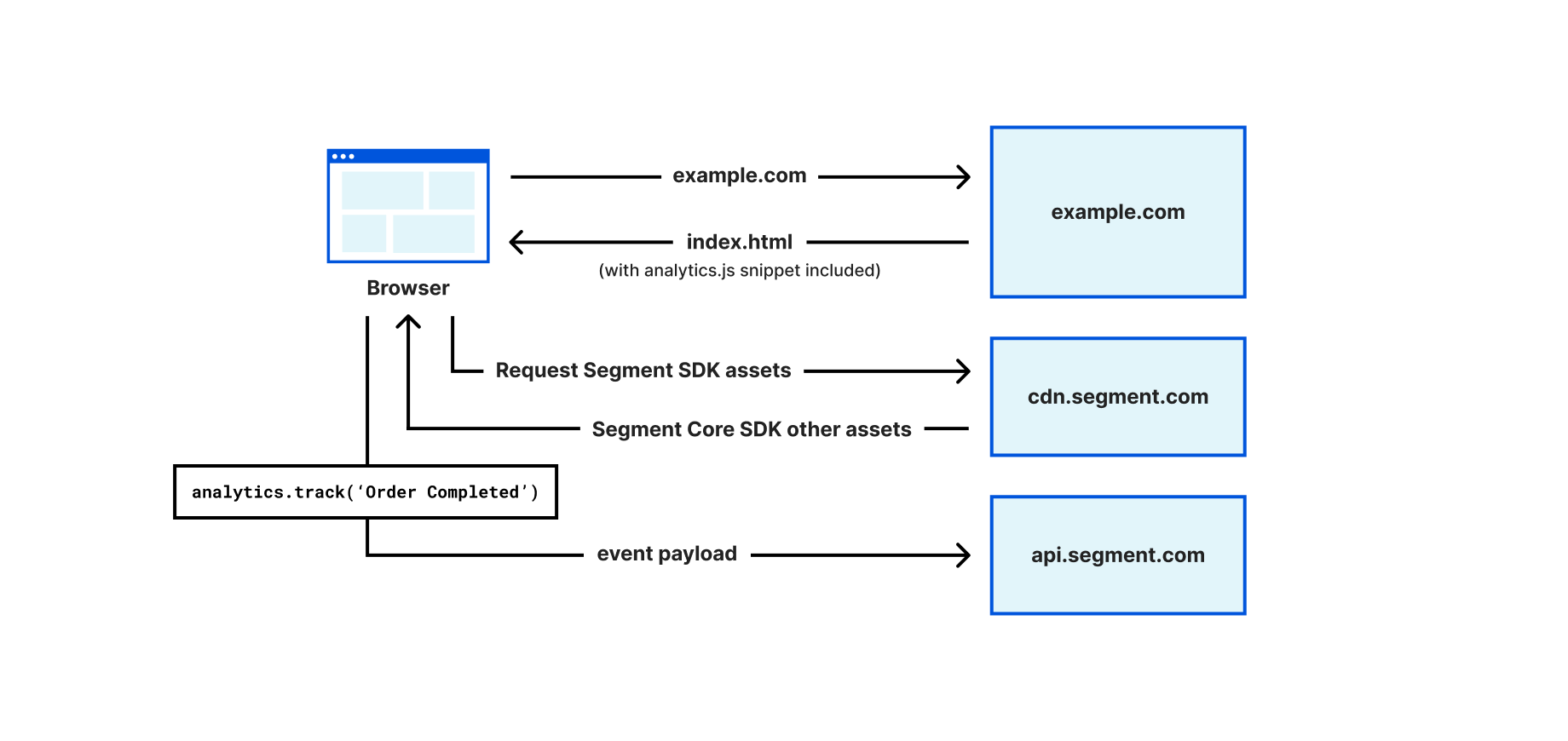
Figure 1 illustrates how Segment can be used to collect data on a web application. Developers add Segment’s web SDK, analytics.js, to their websites by including a JavaScript snippet to the HEAD of their web pages. The snippet can immediately collect and buffer events while it also loads the full library asynchronously from the Segment CDN. Developers can then use analytics.js to identify the visitors, e.g., analytics.identify('john'), and track user behavior, e.g., analytics.track('Order Completed'). Calling the `analytics.js methods such as identify or track will send data to Segment’s API (api.segment.io). Segment’s platform can then deliver the events to different tools, as well as create a profile for the user (e.g., build a profile for user “John”, associate “Order Completed”, as well as add all future activities of john to the profile).

Analytics.js also stores state in the browser as first-party cookies (e.g., storing an ajs_user_id cookie with the value of john, with cookie scoped at the example.com domain) so that when the user visits the website again, the user identifier stored in the cookie can be used to recognize the user.

Twilio Segment Edge SDK Powered by Cloudflare Workers
Figure 1- How analytics.js loads on a website and tracks events

While analytics.js only tracks first-party data (i.e., the data is collected and used by the website that the user is visiting), certain browser controls incorrectly identify analytics.js as a third-party tracker, because the SDK is loaded from a third-party domain (cdn.segment.com) and the data is going to a third-party domain (api.segment.com). Furthermore, despite using first-party cookies to store user identity, some browsers such as Safari have limited the TTL for non-HTTPOnly cookies to 7-days, making it challenging to maintain state for long periods of time.

To overcome these limitations, we have built a Segment Edge SDK (currently in early development) that can automatically add Segment’s library to a web application, eliminate the use of third-party domains, and maintain user identity using HTTPOnly cookies. In the process of solving the first-party data problem, we realized that the Edge SDK is best positioned to act as a personalization library, given it has access to the user identity on every request (in the form of cookies), and it can resolve such identity to a full-user profile stored in Segment. The user profile information can be used to deliver personalized content to users directly from the Cloudflare Workers platform.

The remaining portions of this post will cover how we solved the above problems. We first explain how the Edge SDK helps with first-party collection. Then we cover how the Segment profiles database becomes available on the Cloudflare Workers platform, and how to use such data to drive personalization.

Segment Edge SDK and first-party data collection

Developers can set up the Edge SDK by creating a Cloudflare Worker sitting in front of their web application (via Routes) and importing the Edge SDK via npm. The Edge SDK will handle requests and automatically injects analytics.js snippets into every webpage. It also configures first-party endpoints to download the SDK assets and send tracking data. The Edge SDK also captures user identity by looking at the Segment events and instructs the browser to store such identity as HTTPOnly cookies.

import { Segment } from "@segment/edge-sdk-cloudflare";

export default {
   async fetch(request: Request, env: Env): Promise<Response> {
       const segment = new Segment(env.SEGMENT_WRITE_KEY); 

       const resp = await segment.handleEvent(request, env);

       return resp;
   }
};

How the Edge SDK works under the hood to enable first-party data collection

The Edge SDK’s internal router checks the inbound request URL against predefined patterns. If the URL matches a route, the router runs the route’s chain of handlers to process the request, fetch the origin, or modify the response.

export interface HandlerFunction {
 (
   request: Request,
   response: Response | undefined,
   context: RouterContext
 ): Promise<[Request, Response | undefined, RouterContext]>;
}

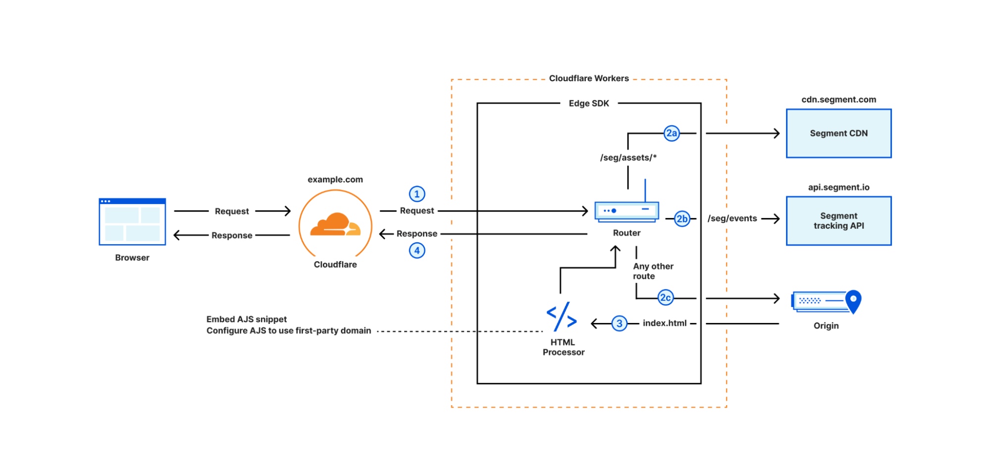
Figure 2 demonstrates the routing of incoming requests. The Worker calls  segment.handleEvent method with the request object (step 1), then the router matches the request.url and request.method against a set of predefined routes:

  • GET requests with /seg/assets/* path are proxied to Segment CDN (step 2a)
  • POST requests with /seg/events/* path are proxied to Segment tracking API (step 2b)
  • Other requests are proxied to the origin (step 2c) and the HTML responses are enriched with the analytics.js snippet (step 3)

Regardless of the route, the router eventually returns a response to the browser (step 4) containing data from the origin, the response from Segment tracking API, or analytics.js assets. When Edge SDK detects the user identity in an incoming request (more on that later), it sets an HTTPOnly cookie in the response headers to persist the user identity in the browser.

Twilio Segment Edge SDK Powered by Cloudflare Workers
Figure 2- Edge SDK router flow‌‌

In the subsequent three sections, we explain how we inject analytics.js, proxy Segment endpoints, and set server-side cookies.

Injecting Segment SDK on requests to origin

For all the incoming requests routed to the origin, the Edge SDK fetches the HTML page and then adds the analytics.js snippet to the <HEAD> tag, embeds the write key, and configures the snippet to download the subsequent javascript bundles from the first-party domain ([first-party host]/seg/assets/*) and sends data to the first-party domain as well ([first-party host]/seg/events/*). This is accomplished using the HTMLRewriter API.

import snippet from "@segment/snippet"; // Existing Segment package that generates snippet

class ElementHandler {
   constructor(host: string, writeKey: string)

   element(element: Element) {
     // generate Segment snippet and configure it with first-party host info
     const snip = snippet.min({
         host: `${this.host}/seg`,
         apiKey: this.writeKey,
       })
     element.append(`<script>${snip}</script>`, { html: true });
   }
 }
  
export const enrichWithAJS: HandlerFunction = async (
   request,
   response,
   context
 ) => {
   const {
     settings: { writeKey },
   } = context;
   const host = request.headers.get("host") || "";
    return [
     request,
     new HTMLRewriter().on("head",
         new ElementHandler(host, writeKey))
       .transform(response),
     context,
   ];
 };

Proxy SDK bundles and Segment API

The Edge SDK proxies the Segment CDN and API under the first-party domain. For example, when the browser loads a page with the injected analytics.js snippet, the snippet loads the full analytics.js bundle from https://example.com/seg/assets/sdk.js, and the Edge SDK will proxy that request to the Segment CDN:

https://cdn.segment.com/analytics.js/v1/<WRITEKEY>/analytics.min.js

export const proxyAnalyticsJS: HandlerFunction = async (request, response, ctx) => {
 const url = `https://cdn.segment.com/analytics.js/v1/${ctx.params.writeKey}/analytics.min.js`;
 const resp = await fetch(url);
 return [request, resp, ctx];
};

Similarly, analytics.js collects events and sends them via a POST request to https://example.com/seg/events/[method] and the Edge SDK will proxy such requests to the Segment tracking API:

https://api.segment.io/v1/[method]

export const handleAPI: HandlerFunction = async (request, response, context) => {
 const url = new URL(request.url);
 const parts = url.pathname.split("/");
 const method = parts.pop();
 let body: { [key: string]: any } = await request.json();

 const init = {
   method: "POST",
   headers: request.headers,
   body: JSON.stringify(body),
 };

 const resp = await fetch(`https://api.segment.io/v1/${method}`, init);

 return [request, resp, context];
};

First party server-side cookies

The Edge SDK also re-writes existing client-side analytics.js cookies as HTTPOnly cookies. When Edge SDK intercepts an identify event e.g., analytics.identify('john'), it extracts the user identity (“john”) and then sets a server-side cookie when sending a response back to the user. Therefore, any subsequent request to the Edge SDK can be associated with “john” using request cookies.

export const enrichResponseWithIdCookies: HandlerFunction = async (
 request, response, context) => {


 const host = request.headers.get("host") || "";
 const body = await request.json();
 const userId = body.userId;

 […]

 const headers = new Headers(response.headers);
 const cookie = cookie.stringify("ajs_user_id", userId, {
   httponly: true,
   path: "/",
   maxage: 31536000,
   domain: host,
 });
 headers.append("Set-Cookie", cookie);
 
 const newResponse = new Response(response.body, {
   ...response,
   headers,
 });

 return [request, newResponse, newContext];
};

Intercepting the ajs_user_id on the Workers, and using the cookie identifier to associate each request to a user, is quite powerful, and it opens the door for delivering personalized content to users. The next section covers how Edge SDK can drive personalization.

Personalization on the Supercloud

The Edge SDK offers a registerVariation method that can customize how a request to a given route should be fetched from the origin. For example, let’s assume we have three versions of a landing page in the origin: /red, /green, and  / (default), and we want to deliver one of the three versions based on the visitor traits. We can use Edge SDK as follows:

   const segment = new Segment(env.SEGMENT_WRITE_KEY); 
   segment.registerVariation("/", (profile) => {
     if (profile.red_group) {
       return "/red"
     } else if (profile.green_group) 
       return "/green"
     }
   });

   const resp = await segment.handleEvent(request, env);

   return resp

The registerVariation accepts two inputs: the path that displays the personalized content, and a decision function that should return the origin address for the personalized content. The decision function receives a profile object visitor in Segment. In the example, when users visit example.com/(root path), personalized content is delivered by checking if the visitor has a red_group or green_group trait and subsequently requesting the content from either /red or /green path at the origin.

We already explained that Edge SDK knows the identity of the user via ajs_user_id cookie, but we haven’t covered how the Edge SDK has access to the full profile object. The next section explains how the full profile becomes available on the Cloudflare Workers platform.

How does personalization work under the hood?

The Personalization feature of the Edge SDK requires storage of profiles on the Cloudflare Workers platform. A Cloudflare KV should be created for the Worker running the Edge SDK and passed to the Edge SDK during initialization. Edge SDK will store profiles in KV, where keys are the ajs_user_id, and values are the serialized profile object. To move Profiles data from Segment to the KV, the SDK uses two methods:

  • Profiles data push from Segment to the Cloudflare Workers platform: The Segment product can sync user profiles database with different tools, including pushing the data to a webhook. The Edge SDK automatically exposes a webhook endpoint under the first-party domain (e.g., example.com/seg/profiles-webhook) that Segment can call periodically to sync user profiles. The webhook handler receives incoming sync calls from Segment, and writes profiles to the KV.
  • Pulling data from Segment by the Edge SDK: If the Edge SDK queries the KV for a user id, and doesn’t find the profile (i.e., data hasn’t synced yet), it requests the user profile from the Segment API, and stores it in the KV.

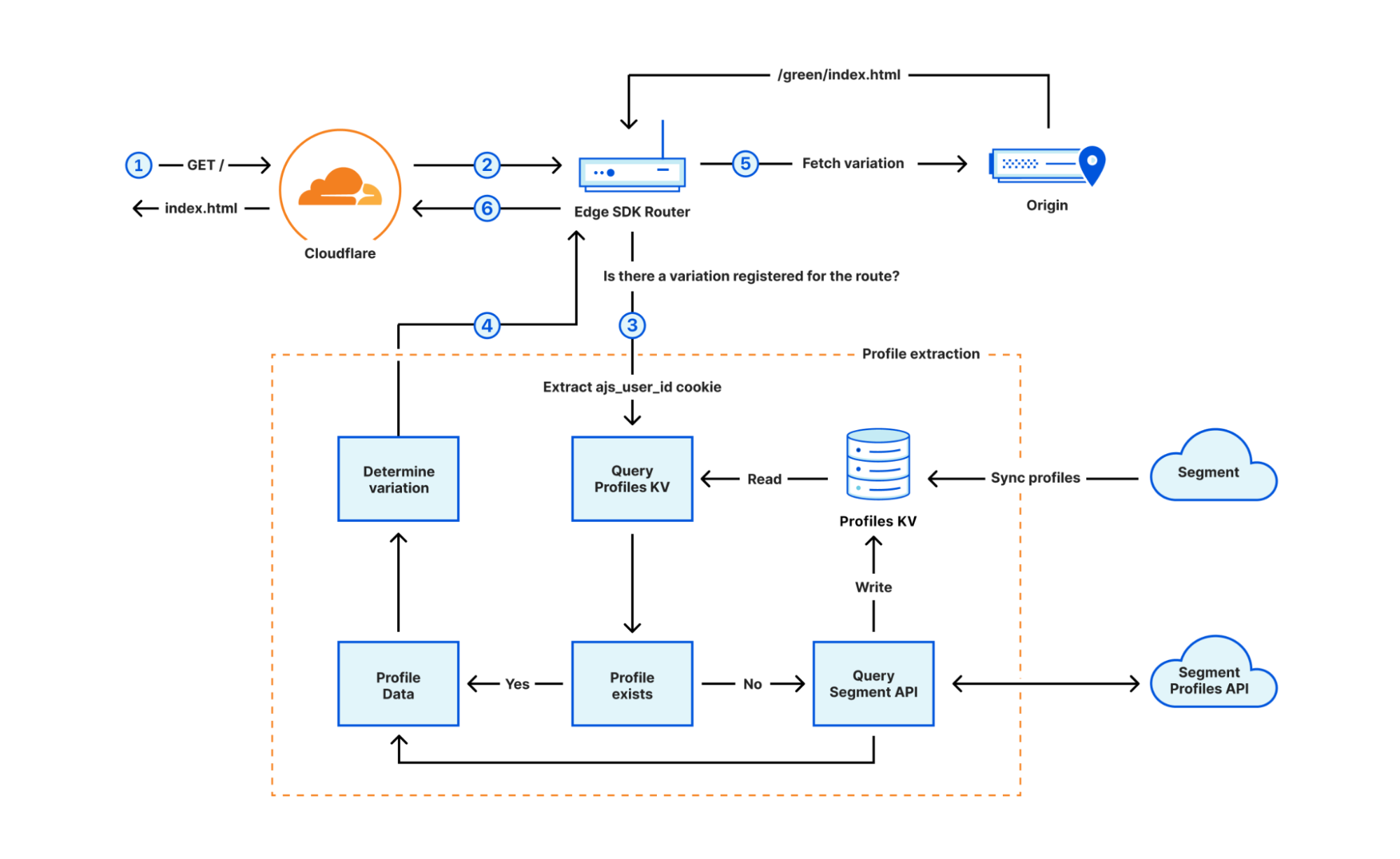
Figure 3 demonstrates how the personalization flow works. In step 1, the user requests content for the root path ( / ), and the Worker sends the request to the Edge SDK (step 2). The Edge SDK router determines that a variation is registered on the route, therefore, extracts the ajs_user_id from the request cookies, and goes through the full profile extraction (step 3). The SDK first checks the KV for a record with the key of ajs_user_id value and if not found, queries Segment API to fetch the profile, and stores the profile in the KV. Eventually, the profile is extracted and passed into the decision function to decide which path should be served to the user (step 4). The router eventually fetches the variation from the origin (step 5) and returns the response under the / path to the browser (step 6).

Twilio Segment Edge SDK Powered by Cloudflare Workers
Figure 3- Personalization flow

Summary

In this post we covered how the Cloudflare Workers platform can help with tracking first-party data and personalization. We also explained how we built a Segment Edge SDK to enable Segment customers to get those benefits out of the box, without having to create their own DIY solution. The Segment Edge SDK is currently in early development, and we are planning to launch a private pilot and open-source it in the near future.

Keep track of Workers’ code and configuration changes with Deployments

Post Syndicated from Kabir Sikand original https://blog.cloudflare.com/deployments-for-workers/

Keep track of Workers’ code and configuration changes with Deployments

Keep track of Workers’ code and configuration changes with Deployments

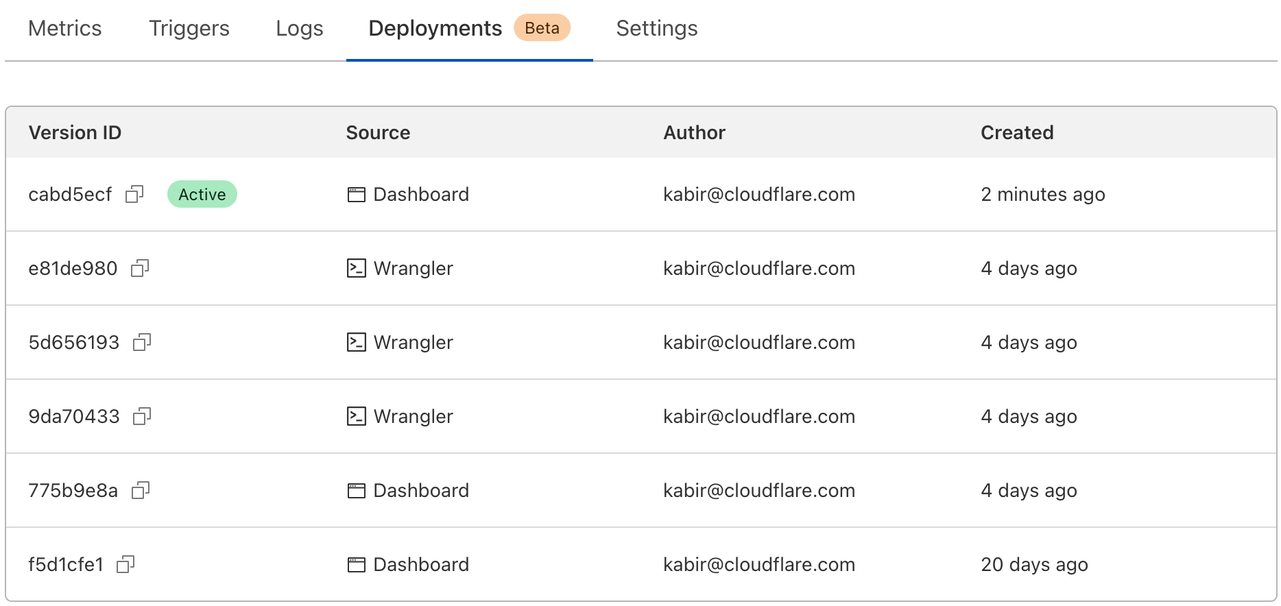
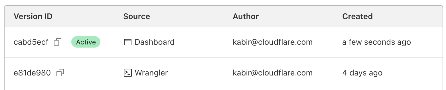
Today we’re happy to introduce Deployments for Workers. Deployments allow developers to keep track of changes to their Worker; not just the code, but the configuration and bindings as well. With deployments, developers now have access to a powerful audit log of changes to their production applications.

And tracking changes is just the beginning! Deployments provide a strong foundation to add: automated deployments, rollbacks, and integration with version control.

Today we’ll dive into the details of deployments, how you can use them, and what we’re thinking about next.

Deployments

Deployments are a powerful new way to track changes to your Workers. With them, you can track who’s making changes to your Workers, where those changes are coming from, and when those changes are being made.

Keep track of Workers’ code and configuration changes with Deployments

Cloudflare reports on deployments made from wrangler, API, dashboard, or Terraform anytime you make changes to your Worker’s code, edit resource bindings and environment variables, or modify configuration like name or usage model.

Keep track of Workers’ code and configuration changes with Deployments

We expose the source of your deployments, so you can track where changes are coming from. For example, if you have a CI job that’s responsible for changes, and you see a user made a change through the Cloudflare dashboard, it’s easy to flag that and dig into whether the deployment was a mistake.

Interacting with deployments

Cloudflare tracks the authors, sources, and timestamps of deployments. If you have a set of users responsible for deployment, or an API Token that’s associated with your CI tool, it’s easy to see which made recent deployments. Each deployment also includes a timestamp, so you can track when those changes were made.

Keep track of Workers’ code and configuration changes with Deployments

You can access all this deployment information in your Cloudflare dashboard, under your Worker’s Deployments tab. We also report on the active version right at the front of your Worker’s detail page. Wrangler will also report on deployment information. wrangler publish now reports the latest deployed version, and a new `wrangler deployments` command can be used to view a deployment history.

Keep track of Workers’ code and configuration changes with Deployments

To learn more about the details of deployments, head over to our Developer Documentation.

What’s next?

We’re excited to share deployments with our customers, available today in an open beta. As we mentioned up front, we’re just getting started with deployments. We’re also excited for more on-platform tooling like rollbacks, deploy status, deployment rules, and a view-only mode to historical deployments. Beyond that, we want to ensure deployments can be automated from commits to your repository, which means working on version control integrations to services like GitHub, Bitbucket, and Gitlab. We’d love to hear more about how you’re currently using Workers and how we can improve developer experience. If you’re interested, let’s chat.

If you’d like to join the conversation, head over to Cloudflare’s Developer Discord and give us a shout! We love hearing from our customers, and we’re excited to see what you build with Cloudflare.

Best Practices for Hosting Regulated Gaming Workloads in AWS Local Zones and on AWS Outposts

Post Syndicated from Sheila Busser original https://aws.amazon.com/blogs/compute/best-practices-for-hosting-regulated-gaming-workloads-in-aws-local-zones-and-on-aws-outposts/

This blog post is written by Shiv Bhatt, Manthan Raval, and Pawan Matta, who are Senior Solutions Architects with AWS.

Many industries are subject to regulations that are created to protect the interests of the various stakeholders. For some industries, the specific details of the regulatory requirements influence not only the organization’s operations, but also their decisions for adopting new technology. In this post, we highlight the workload residency challenges that you may encounter when you deploy regulated gaming workloads, and how AWS Local Zones and AWS Outposts can help you address those challenges.

Regulated gaming workloads and residency requirements

A regulated gaming workload is a type of workload that’s subject to federal, state, local, or tribal laws related to the regulation of gambling and real money gaming. Examples of these workloads include sports betting, horse racing, casino, poker, lottery, bingo, and fantasy sports. The operators provide gamers with access to these workloads through online and land-based channels, and they’re required to follow various regulations required in their jurisdiction. Some regulations define specific workload residency requirements, and depending on the regulatory agency, the regulations could require that workloads be hosted within a specific city, state, province, or country. For example, in the United States, different state and tribal regulatory agencies dictate whether and where gaming operations are legal in a state, and who can operate. The agencies grant licenses to the operators of regulated gaming workloads, which then govern who can operate within the state, and sometimes, specifically where these workloads can be hosted. In addition, federal legislation can also constrain how regulated gaming workloads can be operated. For example, the United States Federal Wire Act makes it illegal to facilitate bets or wagers on sporting events across state lines. This regulation requires that operators make sure that users who place bets in a specific state are also within the borders of that state.

Benefits of using AWS edge infrastructure with regulated gaming workloads

The use of AWS edge infrastructure, specifically Local Zones and Outposts to host a regulated gaming workload, can help you meet workload residency requirements. You can manage Local Zones and Outposts by using the AWS Management Console or by using control plane API operations, which lets you seamlessly consume compute, storage, and other AWS services.

Local Zones

Local Zones are a type of AWS infrastructure deployment that place compute, storage, database, and other select services closer to large population, industry, and IT centers. Like AWS Regions, Local Zones enable you to innovate more quickly and bring new products to market sooner without having to worry about hardware and data center space procurement, capacity planning, and other forms of undifferentiated heavy-lifting. Local Zones have their own connections to the internet, and support AWS Direct Connect, so that workloads hosted in the Local Zone can serve local end-users with very low-latency communications. Local Zones are by default connected to a parent Region via Amazon’s redundant and high-bandwidth private network. This lets you extend Amazon Virtual Private Cloud (Amazon VPC) in the AWS Region to Local Zones. Furthermore, this provides applications hosted in AWS Local Zones with fast, secure, and seamless access to the broader portfolio of AWS services in the AWS Region. You can see the full list of AWS services supported in Local Zones on the AWS Local Zones features page.

You can start using Local Zones right away by enabling them in your AWS account. There are no setup fees, and as with the AWS Region, you pay only for the services that you use. There are three ways to pay for Amazon Elastic Compute Cloud (Amazon EC2) instances in Local Zones: On-Demand, Savings Plans, and Spot Instances. See the full list of cities where Local Zones are available on the Local Zones locations page.

Outposts

Outposts is a family of fully-managed solutions that deliver AWS infrastructure and services to most customer data center locations for a consistent hybrid experience. For a full list of countries and territories where Outposts is available, see the Outposts rack FAQs and Outposts servers FAQs. Outposts is available in various form factors, from 1U and 2U Outposts servers to 42U Outposts racks, and multiple rack deployments. To learn more about specific configuration options and pricing, see Outposts rack and Outposts servers.

You configure Outposts to work with a specific AWS Region using AWS Direct Connect or an internet connection, which lets you extend Amazon VPC in the AWS Region to Outposts. Like Local Zones, this provides applications hosted on Outposts with fast, secure, and seamless access to the broader portfolio of AWS services in the AWS Region. See the full list of AWS services supported on Outposts rack and on Outposts servers.

Choosing between AWS Regions, Local Zones, and Outposts

When you build and deploy a regulated gaming workload, you must assess the residency requirements carefully to make sure that your workload complies with regulations. As you make your assessment, we recommend that you consider separating your regulated gaming workload into regulated and non-regulated components. For example, for a sports betting workload, the regulated components might include sportsbook operation, and account and wallet management, while non-regulated components might include marketing, the odds engine, and responsible gaming. In describing the following scenarios, it’s assumed that regulated and non-regulated components must be fault-tolerant.

For hosting the non-regulated components of your regulated gaming workload, we recommend that you consider using an AWS Region instead of a Local Zone or Outpost. An AWS Region offers higher availability, larger scale, and a broader selection of AWS services.

For hosting regulated components, the type of AWS infrastructure that you choose will depend on which of the following scenarios applies to your situation:

  1. Scenario one: An AWS Region is available in your jurisdiction and local regulators have approved the use of cloud services for your regulated gaming workload.
  2. Scenario two: An AWS Region isn’t available in your jurisdiction, but a Local Zone is available, and local regulators have approved the use of cloud services for your regulated gaming workload.
  3. Scenario three: An AWS Region or Local Zone isn’t available in your jurisdiction, or local regulators haven’t approved the use of cloud services for your regulated gaming workload, but Outposts is available.

Let’s look at each of these scenarios in detail.

Scenario one: Use an AWS Region for regulated components

When local regulators have approved the use of cloud services for regulated gaming workloads, and an AWS Region is available in your jurisdiction, consider using an AWS Region rather than a Local Zone and Outpost. For example, in the United States, the State of Ohio has announced that it will permit regulated gaming workloads to be deployed in the cloud on infrastructure located within the state when sports betting goes live in January 2023. By using the US East (Ohio) Region, operators in the state don’t need to procure and manage physical infrastructure and data center space. Instead, they can use various compute, storage, database, analytics, and artificial intelligence/machine learning (AI/ML) services that are readily available in the AWS Region. You can host a regulated gaming workload entirely in a single AWS Region, which includes Availability Zones (AZs) – multiple, isolated locations within each AWS Region. By deploying your workload redundantly across at least two AZs, you can help make sure of the high availability, as shown in the following figure.

AWS Region hosting regulated and non-regulated components

Scenario two: Use a Local Zone for regulated components

A second scenario might be that local regulators have approved the use of cloud services for regulated gaming workloads, and an AWS Region isn’t available in your jurisdiction, but a Local Zone is available. In this scenario, consider using a Local Zone rather than Outposts. A Local Zone can support more elasticity in a more cost-effective way than Outposts can. However, you might also consider using a Local Zone and Outposts together to increase availability and scalability for regulated components. Let’s consider the State of Illinois, in the United States, which allows regulated gaming workloads to be deployed in the cloud, if workload residency requirements are met. Operators in this state can host regulated components in a Local Zone in Chicago, and they can also use Outposts in their data center in the same state, for high availability and disaster recovery, as shown in the following figure.

Route ingress gaming traffic through an AWS Region hosting non-regulated components, with a Local Zone and Outposts hosting regulated components

Scenario three: Use of Outposts for regulated components

When local regulators haven’t approved the use of cloud services for regulated gaming workloads, or when an AWS Region or Local Zone isn’t available in your jurisdiction, you can still choose to host your regulated gaming workloads on Outposts for a consistent cloud experience, if Outposts is available in your jurisdiction. If you choose to use Outposts, then note that as part of the shared responsibility model, customers are responsible for attesting to physical security and access controls around the Outpost, as well as environmental requirements for the facility, networking, and power. Use of Outposts requires you to procure and manage the data center within the city, state, province, or country boundary (as required by local regulations) that may be suitable to host regulated components, depending on the jurisdiction. Furthermore, you should procure and configure supported network connections between Outposts and the parent AWS Region. During the Outposts ordering process, you should account for the compute and network capacity required to support the peak load and availability design.

For a higher availability level, you should consider procuring and deploying two or more Outposts racks or Outposts servers in a data center. You might also consider deploying redundant network paths between Outposts and the parent AWS Region. However, depending on your business service level agreement (SLA) for regulated gaming workload, you might choose to spread Outposts racks across two or more isolated data centers within the same regulated boundary, as shown in the following figure.

Route ingress gaming traffic through an AWS Region hosting non-regulated components, with an Outposts hosting regulated components

Options to route ingress gaming traffic

You have two options to route ingress gaming traffic coming into your regulated and non-regulated components when you deploy the configurations that we described previously in Scenarios two and three. Your gaming traffic can come through to the AWS Region, or through the Local Zones or Outposts. Note that the benefits that we mentioned previously around selecting the AWS Region for deploying regulated and non-regulated components are the same when you select an ingress route.

Let’s discuss the benefits and trade offs for each of these options.

Option one: Route ingress gaming traffic through an AWS Region

If you choose to route ingress gaming traffic through an AWS Region, your regulated gaming workloads benefit from access to the wide range of tools, services, and capacity available in the AWS Region. For example, native AWS security services, like AWS WAF and AWS Shield, which provide protection against DDoS attacks, are currently only available in AWS Regions. Only traffic that you route into your workload through an AWS Region benefits from these services.

If you route gaming traffic through an AWS Region, and non-regulated components are hosted in an AWS Region, then traffic has a direct path to non-regulated components. In addition, gaming traffic destined to regulated components, hosted in a Local Zone and on Outposts, can be routed through your non-regulated components and a few native AWS services in the AWS Region, as shown in Figure 2.

Option two: Route ingress gaming traffic through a Local Zone or Outposts

Choosing to route ingress gaming traffic through a Local Zone or Outposts requires careful planning to make sure that tools, services, and capacity are available in that jurisdiction, as shown in the following figure. In addition, consider how choosing this route will influence the pillars of the AWS Well-Architected Framework. This route might require deploying and managing most of your non-regulated components in a Local Zone or on Outposts as well, including native AWS services that aren’t available in Local Zones or on Outposts. If you plan to implement this topology, then we recommend that you consider using AWS Partner solutions to replace the native AWS services that aren’t available in Local Zones or Outposts.

Route ingress gaming traffic through a Local Zone and Outposts that are hosting regulated and non-regulated components, with an AWS Region hosting limited non-regulated components

Conclusion

If you’re building regulated gaming workloads, then you might have to follow strict workload residency and availability requirements. In this post, we’ve highlighted how Local Zones and Outposts can help you meet these workload residency requirements by bringing AWS services closer to where they’re needed. We also discussed the benefits of using AWS Regions in compliment to the AWS edge infrastructure, and several reliability and cost design considerations.

Although this post provides information to consider when making choices about using AWS for regulated gaming workloads, you’re ultimately responsible for maintaining compliance with the gaming regulations and laws in your jurisdiction. You’re in the best position to determine and maintain ultimate responsibility for determining whether activities are legal, including evaluating the jurisdiction of the activities, how activities are made available, and whether specific technologies or services are required to make sure of compliance with the applicable law. You should always review these regulations and laws before you deploy regulated gaming workloads on AWS.

Build your next big idea with Cloudflare Pages

Post Syndicated from Nevi Shah original https://blog.cloudflare.com/big-ideas-on-pages/

Build your next big idea with Cloudflare Pages

Build your next big idea with Cloudflare Pages

Have you ever had a surge of inspiration for a project? That feeling when you have a great idea – a big idea — that you just can’t shake? When all you can think about is putting your hands to your keyboard and hacking away? Building a website takes courage, creativity, passion and drive, and with Cloudflare Pages we believe nothing should stand in the way of that vision.

Especially not a price tag.

Big ideas

We built Pages to be at the center of your developer experience – a way for you to get started right away without worrying about the heavy lift of setting up a fullstack app.  A quick commit to your git provider or direct upload to our platform, and your rich and powerful site is deployed to our network of 270+ data centers in seconds. And above all, we built Pages to scale with you as you grow exponentially without getting hit by an unexpected bill.

The limit does not exist

We’re a platform that’s invested in your vision – no matter how wacky and wild (the best ones usually are!). That’s why for many parts of Pages we want your experience to be limitless.

Unlimited requests: As your idea grows, so does your traffic. While thousands and millions of end users flock to your site, Pages is prepared to handle all of your traffic with no extra cost to you – even when millions turn to billions.

Unlimited bandwidth: As your traffic grows, you’ll need more bandwidth – and with Pages, we got you. If your site takes off in popularity one day, the next day shouldn’t be a cause for panic because of a nasty bill. It should be a day of celebration and pride. We’re giving unlimited bandwidth so you can keep your eyes focused on moving up and to the right.

Unlimited free seats: With a rise in demand for your app, you’re going to need more folks working with you. We know from experience that more great ideas don’t just come from one person but a strong team of people. We want to be there every step of the way along with every person you want on this journey with you. Just because your team grows doesn’t mean your bill has to.

Unlimited projects: With one great idea, means many more to follow. With Pages, you can deploy as many projects as you want – keep them coming! Not every idea is going to be the right one – we know this! Prove out your vision in private org-owned repos for free! Try out a plethora of development frameworks until you’ve found the perfect combination for your idea. Test your changes locally using our Wrangler integration so you can be confident in whatever you choose to put out into the world.

Quick, easy and free integrations

Workers: Take your idea from static to dynamic with Pages’ native integration with Cloudflare Workers, our serverless functions offering. Drop your functions into your functions folder and deploy them alongside your static assets no extra configuration required! We announced built-in support for Cloudflare Workers back in November and have since announced framework integrations with Remix, Sveltekit and Qwik, and are working on fullstack support for Next.js within the year!

Cloudflare Access: Working with more than just a team of developers? Send your staging changes to product managers and marketing teams with a unique preview URL for every deployment. And what’s more? You can enable protection for your preview links using our native integration with Cloudflare Access at no additional cost. With one click, send around your latest version without fear of getting into the wrong hands.

Custom domains: With every Pages project, get a free pages.dev subdomain to deploy your project under. When you’re ready for the big day, with built in SSL for SaaS, bring that idea to life with a custom domain of its own!

Web Analytics: When launch day comes around, check out just how well it’s going with our deep, privacy-first integration with Cloudflare’s Web Analytics. Track every single one of your sites’ progress and performance, including metrics about your traffic and core web vitals with just one click – completely on us!

Wicked fast performance

And the best part? Our generous free tier never means compromising site performance. Bring your site closer to your users on your first deployment no matter where they are in the world. The Cloudflare network spans across 270+ cities around the globe and your site is distributed to each of them faster than you can say “it’s go time”. There’s also no need to choose regions for your deployments, we want you to have them all and get even more granular, so your big idea can truly go global.

What else?

Building on Pages is just the start of what your idea could grow to become. In the coming months you can expect deep integrations with our new Cloudflare storage offerings like R2, our object storage service with zero egress fees (open beta), and D1 our first SQL database on the edge (private beta).

We’ve talked a lot about building your entire platform on Cloudflare. We’re reimagining this experience to be even easier and even more powerful.

Using just Cloudflare, you’ll be able to build big projects – like an entire store! You can use R2 to host the images, D1 to store product info, inventory data and user details, and Pages to seamlessly build and deploy. A frictionless dev experience for a full stack app that can live and work entirely from the edge. Best of all, don’t worry about getting hung up on cost, we’ll always have a generous free tier so you can get started right away.

At Cloudflare, we believe that every developer deserves to dream big. For the developers who love to build, who are curious, who explore, let us take you there – no surprises! Leave the security and scalability to us, so you can put your fingers to the keyboard and do what you do best!

Give it a go

Learn more about Pages and check out our developer documentation. Be sure to join our active Cloudflare Developer Discord and meet our community of developers building on our platform. You can chat directly with our product and engineering teams and get exclusive access to our offered betas!
Building scheduling system with Workers and Durable Objects

Post Syndicated from Adam Janiš original https://blog.cloudflare.com/building-scheduling-system-with-workers-and-durable-objects/

Building scheduling system with Workers and Durable Objects

Building scheduling system with Workers and Durable Objects

We rely on technology to help us on a daily basis – if you are not good at keeping track of time, your calendar can remind you when it’s time to prepare for your next meeting. If you made a reservation at a really nice restaurant, you don’t want to miss it! You appreciate the app to remind you a day before your plans the next evening.
However, who tells the application when it’s the right time to send you a notification? For this, we generally rely on scheduled events. And when you are relying on them, you really want to make sure that they occur. Turns out, this can get difficult. The scheduler and storage backend need to be designed with scale in mind – otherwise you may hit limitations quickly.

Workers, Durable Objects, and Alarms are actually a perfect match for this type of workload. Thanks to the distributed architecture of Durable Objects and their storage, they are a reliable and scalable option. Each Durable Object has access to its own isolated storage and alarm scheduler, both being automatically replicated and failover in case of failures.

There are many use cases where having a reliable scheduler can come in handy: running a webhook service, sending emails to your customers a week after they sign up to keep them engaged, sending invoices reminders, and more!

Today, we’re going to show you how to build a scalable service that will schedule HTTP requests on a specific schedule or as one-off at a specific time as a way to guide you through any use case that requires scheduled events.

Building scheduling system with Workers and Durable Objects

Quick intro into the application stack

Before we dive in, here are some of the tools we’re going to be using today:

The application is going to have following components:

  • Scheduling system API to accept scheduled requests and manage Durable Objects
  • Unique Durable Object per scheduled request, each with
  • Storage – keeping the request metadata, such as URL, body, or headers.
  • Alarm – a timer (trigger) to wake Durable Object up.

While we will focus on building the application, the Cloudflare global network will take care of the rest – storing and replicating our data, and making sure to wake our Durable Objects up when the time’s right. Let’s build it!

Initialize new Workers project

Get started by generating a completely new Workers project using the wrangler init command, which makes creating new projects quick & easy.

wrangler init -y durable-objects-requests-scheduler

Building scheduling system with Workers and Durable Objects

For more information on how to install, authenticate, or update Wrangler, check out https://developers.cloudflare.com/workers/wrangler/get-started

Preparing TypeScript types

From my personal experience, at least a draft of TypeScript types significantly helps to be more productive down the road, so let’s prepare and describe our scheduled request in advance. Create a file types.ts in src directory and paste the following TypeScript definitions.

src/types.ts

export interface Env {
    DO_REQUEST: DurableObjectNamespace
}
 
export interface ScheduledRequest {
  url: string // URL of the request
  triggerAt?: number // optional, unix timestamp in milliseconds, defaults to `new Date()`
  requestInit?: RequestInit // optional, includes method, headers, body
}

A scheduled request Durable Object class & alarm

Based on our architecture design, each scheduled request will be saved into its own Durable Object, effectively separating storage and alarms from each other and allowing our scheduling system to scale horizontally – there is no limit to the number of Durable Objects we create.

In the end, the Durable Object class is a matter of a couple of lines. The code snippet below accepts and saves the request body to a persistent storage and sets the alarm timer. Workers runtime will wake up the Durable Object and call the alarm() method to process the request.

The alarm method reads the scheduled request data from the storage, then processes the request, and in the end reschedules itself in case it’s configured to be executed on a recurring schedule.

src/request-durable-object.ts

import { ScheduledRequest } from "./types";
 
export class RequestDurableObject {
  id: string|DurableObjectId
  storage: DurableObjectStorage
 
  constructor(state:DurableObjectState) {
    this.storage = state.storage
    this.id = state.id
  }
 
    async fetch(request:Request) {
    // read scheduled request from request body
    const scheduledRequest:ScheduledRequest = await request.json()
     
    // save scheduled request data to Durable Object storage, set the alarm, and return Durable Object id
    this.storage.put("request", scheduledRequest)
    this.storage.setAlarm(scheduledRequest.triggerAt || new Date())
    return new Response(JSON.stringify({
      id: this.id.toString()
    }), {
      headers: {
        "content-type": "application/json"
      }
    })
  }
 
  async alarm() {
    // read the scheduled request from Durable Object storage
    const scheduledRequest:ScheduledRequest|undefined = await this.storage.get("request")
 
    // call fetch on scheduled request URL with optional requestInit
    if (scheduledRequest) {
      await fetch(scheduledRequest.url, scheduledRequest.requestInit ? webhook.requestInit : undefined)
 
      // cleanup scheduled request once done
      this.storage.deleteAll()
    }
  }
}

Wrangler configuration

Once we have the Durable Object class, we need to create a Durable Object binding by instructing Wrangler where to find it and what the exported class name is.

wrangler.toml

name = "durable-objects-request-scheduler"
main = "src/index.ts"
compatibility_date = "2022-08-02"
 
# added Durable Objects configuration
[durable_objects]
bindings = [
  { name = "DO_REQUEST", class_name = "RequestDurableObject" },
]
 
[[migrations]]
tag = "v1"
new_classes = ["RequestDurableObject"]

Scheduling system API

The API Worker will accept POST HTTP methods only, and is expecting a JSON body with scheduled request data – what URL to call, optionally what method, headers, or body to send. Any other method than POST will return 405 – Method Not Allowed HTTP error.

HTTP POST /:scheduledRequestId? will create or override a scheduled request, where :scheduledRequestId is optional Durable Object ID returned from a scheduling system API before.

src/index.ts

import { Env } from "./types"
export { RequestDurableObject } from "./request-durable-object"
 
export default {
    async fetch(
        request: Request,
        env: Env
    ): Promise<Response> {
        if (request.method !== "POST") {
            return new Response("Method Not Allowed", {status: 405})
        }
 
        // parse the URL and get Durable Object ID from the URL
        const url = new URL(request.url)
        const idFromUrl = url.pathname.slice(1)
 
        // construct the Durable Object ID, use the ID from pathname or create a new unique id
        const doId = idFromUrl ? env.DO_REQUEST.idFromString(idFromUrl) : env.DO_REQUEST.newUniqueId()
 
        // get the Durable Object stub for our Durable Object instance
        const stub = env.DO_REQUEST.get(doId)
 
        // pass the request to Durable Object instance
        return stub.fetch(request)
    },
}

It’s good to mention that the script above does not implement any listing of scheduled or processed webhooks. Depending on how the scheduling system would be integrated, you can save each created Durable Object ID to your existing backend, or write your own registry – using one of the Workers storage options.

Starting a local development server and testing our application

We are almost done! Before we publish our scheduler system to the Cloudflare edge, let’s start Wrangler in a completely local mode to run a couple of tests against it and to see it in action – which will work even without an Internet connection!

wrangler dev --local
Building scheduling system with Workers and Durable Objects

The development server is listening on localhost:8787, which we will use for scheduling our first request. The JSON request payload should match the TypeScript schema we defined in the beginning – required URL, and optional triggerEverySeconds number or triggerAt unix timestamp. When only the required URL is passed, the request will be dispatched right away.

An example of request payload that will send a GET request to https://example.com every 30 seconds.

{
	"url":  "https://example.com",
	"triggerEverySeconds": 30,
}
> curl -X POST -d '{"url": "https://example.com", "triggerEverySeconds": 30}' http://localhost:8787
{"id":"000000018265a5ecaa5d3c0ab6a6997bf5638fdcb1a8364b269bd2169f022b0f"}
Building scheduling system with Workers and Durable Objects

From the wrangler logs we can see the scheduled request ID 000000018265a5ecaa5d3c0ab6a6997bf5638fdcb1a8364b269bd2169f022b0f is being triggered in 30s intervals.

Need to double the interval? No problem, just send a new POST request and pass the request ID as a pathname.

> curl -X POST -d '{"url": "https://example.com", "triggerEverySeconds": 60}' http://localhost:8787/000000018265a5ecaa5d3c0ab6a6997bf5638fdcb1a8364b269bd2169f022b0f
{"id":"000000018265a5ecaa5d3c0ab6a6997bf5638fdcb1a8364b269bd2169f022b0f"}

Every scheduled request gets a unique Durable Object ID with its own storage and alarm. As we demonstrated, the ID becomes handy when you need to change the settings of the scheduled request, or to deschedule them completely.

Publishing to the network

Following command will bundle our Workers application, export and bind Durable Objects, and deploy it to our workers.dev subdomain.

wrangler publish
Building scheduling system with Workers and Durable Objects

That’s it, we are live! 🎉 The URL of your deployment is shown in the Workers logs. In a reasonably short period of time we managed to write our own scheduling system that is ready to handle requests at scale.

You can check full source code in Workers templates repository, or experiment from your browser without installing any dependencies locally using the StackBlitz template.

What to see or build next

An introduction to three-phase power and PDUs

Post Syndicated from Rob Dinh original https://blog.cloudflare.com/an-introduction-to-three-phase-power-and-pdus/

An introduction to three-phase power and PDUs

Our fleet of over 200 locations comprises various generations of servers and routers. And with the ever changing landscape of services and computing demands, it’s imperative that we manage power in our data centers right. This blog is a brief Electrical Engineering 101 session going over specifically how power distribution units (PDU) work, along with some good practices on how we use them. It appears to me that we could all use a bit more knowledge on this topic, and more love and appreciation of something that’s critical but usually taken for granted, like hot showers and opposable thumbs.

A PDU is a device used in data centers to distribute power to multiple rack-mounted machines. It’s an industrial grade power strip typically designed to power an average consumption of about seven US households. Advanced models have monitoring features and can be accessed via SSH or webGUI to turn on and off power outlets. How we choose a PDU depends on what country the data center is and what it provides in terms of voltage, phase, and plug type.

An introduction to three-phase power and PDUs

For each of our racks, all of our dual power-supply (PSU) servers are cabled to one of the two vertically mounted PDUs. As shown in the picture above, one PDU feeds a server’s PSU via a red cable, and the other PDU feeds that server’s other PSU via a blue cable. This is to ensure we have power redundancy maximizing our service uptime; in case one of the PDUs or server PSUs fail, the redundant power feed will be available keeping the server alive.

Faraday’s Law and Ohm’s Law

Like most high-voltage applications, PDUs and servers are designed to use AC power. Meaning voltage and current aren’t constant — they’re sine waves with magnitudes that can alternate between positive and negative at a certain frequency. For example, a voltage feed of 100V is not constantly at 100V, but it bounces between 100V and -100V like a sine wave. One complete sine wave cycle is one phase of 360 degrees, and running at 50Hz means there are 50 cycles per second.

The sine wave can be explained by Faraday’s Law and by looking at how an AC power generator works. Faraday’s Law tells us that a current is induced to flow due to a changing magnetic field. Below illustrates a simple generator with a permanent magnet rotating at constant speed and a coil coming in contact with the magnet’s magnetic field. Magnetic force is strongest at the North and South ends of the magnet. So as it rotates on itself near the coil, current flow fluctuates in the coil. One complete rotation of the magnet represents one phase. As the North end approaches the coil, current increases from zero. Once the North end leaves, current decreases to zero. The South end in turn approaches, now the current “increases” in the opposite direction. And finishing the phase, the South end leaves returning the current back to zero. Current alternates its direction at every half cycle, hence the naming of Alternating Current.

An introduction to three-phase power and PDUs

Current and voltage in AC power fluctuate in-phase, or “in tandem”, with each other. So by Ohm’s Law of Power = Voltage x Current, power will always be positive. Notice on the graph below that AC power (Watts) has two peaks per cycle. But for practical purposes, we’d like to use a constant power value. We do that by interpreting AC power into “DC” power using root-mean-square (RMS) averaging, which takes the max value and divides it by √2. For example, in the US, our conditions are 208V 24A at 60Hz. When we look at spec sheets, all of these values can be assumed as RMS’d into their constant DC equivalent values. When we say we’re fully utilizing a PDU’s max capacity of 5kW, it actually means that the power consumption of our machines bounces between 0 and 7.1kW (5kW x √2).

An introduction to three-phase power and PDUs

It’s also critical to figure out the sum of power our servers will need in a rack so that it falls under the PDU’s design max power capacity. For our US example, a PDU is typically 5kW (208 volts x 24 amps); therefore, we’re budgeting 5kW and fit as many machines as we can under that. If we need more machines and the total sum power goes above 5kW, we’d need to provision another power source. That would lead to possibly another set of PDUs and racks that we may not fully use depending on demand; e.g. more underutilized costs. All we can do is abide by P = V x I.

However there is a way we can increase the max power capacity economically — 3-phase PDU. Compared to single phase, its max capacity is √3 or 1.7 times higher. A 3-phase PDU of the same US specs above has a capacity of 8.6kW (5kW x √3), allowing us to power more machines under the same source. Using a 3-phase setup might mean it has thicker cables and bigger plug; but despite being more expensive than a 1-phase, its value is higher compared to two 1-phase rack setups for these reasons:

  • It’s more cost-effective, because there are fewer hardware resources to buy
  • Say the computing demand adds up to 215kW of hardware, we would need 25 3-phase racks compared to 43 1-phase racks.
  • Each rack needs two PDUs for power redundancy. Using the example above, we would need 50 3-phase PDUs compared to 86 1-phase PDUs to power 215kW worth of hardware.
  • That also means a smaller rack footprint and fewer power sources provided and charged by the data center, saving us up to √3 or 1.7 times in opex.
  • It’s more resilient, because there are more circuit breakers in a 3-phase PDU — one more than in a 1-phase. For example, a 48-outlet PDU that is 1-phase would be split into two circuits of 24 outlets. While a 3-phase one would be split into 3 circuits of 16 outlets. If a breaker tripped, we’d lose 16 outlets using a 3-phase PDU instead of 24.
An introduction to three-phase power and PDUs

The PDU shown above is a 3-phase model of 48 outlets. We can see three pairs of circuit breakers for the three branches that are intertwined with each other — white, grey, and black. Industry demands today pressure engineers to maximize compute performance and minimize physical footprint, making the 3-phase PDU a widely-used part of operating a data center.

What is 3-phase?

A 3-phase AC generator has three coils instead of one where the coils are 120 degrees apart inside the cylindrical core, as shown in the figure below. Just like the 1-phase generator, current flow is induced by the rotation of the magnet thus creating power from each coil sequentially at every one-third of the magnet’s rotation cycle. In other words, we’re generating three 1-phase power offset by 120 degrees.

An introduction to three-phase power and PDUs

A 3-phase feed is set up by joining any of its three coils into line pairs. L1, L2, and L3 coils are live wires with each on their own phase carrying their own phase voltage and phase current. Two phases joining together form one line carrying a common line voltage and line current. L1 and L2 phase voltages create the L1/L2 line voltage. L2 and L3 phase voltages create the L2/L3 line voltage. L1 and L3 phase voltages create the L1/L3 line voltage.

An introduction to three-phase power and PDUs

Let’s take a moment to clarify the terminology. Some other sources may refer to line voltage (or current) as line-to-line or phase-to-phase voltage (or current). It can get confusing, because line voltage is the same as phase voltage in 1-phase circuits, as there’s only one phase. Also, the magnitude of the line voltage is equal to the magnitude of the phase voltage in 3-phase Delta circuits, while the magnitude of the line current is equal to the magnitude of the phase current in 3-phase Wye circuits.

Conversely, the line current equals to phase current times √3 in Delta circuits. In Wye circuits, the line voltage equals to phase voltage times √3.

In Delta circuits:
Vline = Vphase
Iline = √3 x Iphase

In Wye circuits:
Vline = √3 x Vphase
Iline = Iphase

Delta and Wye circuits are the two methods that three wires can join together. This happens both at the power source with three coils and at the PDU end with three branches of outlets. Note that the generator and the PDU don’t need to match each other’s circuit types.

An introduction to three-phase power and PDUs

On PDUs, these phases join when we plug servers into the outlets. So we conceptually use the wirings of coils above and replace them with resistors to represent servers. Below is a simplified wiring diagram of a 3-phase Delta PDU showing the three line pairs as three modular branches. Each branch carries two phase currents and its own one common voltage drop.

An introduction to three-phase power and PDUs

And this one below is of a 3-phase Wye PDU. Note that Wye circuits have an additional line known as the neutral line where all three phases meet at one point. Here each branch carries one phase and a neutral line, therefore one common current. The neutral line isn’t considered as one of the phases.

An introduction to three-phase power and PDUs

Thanks to a neutral line, a Wye PDU can offer a second voltage source that is √3 times lower for smaller devices, like laptops or monitors. Common voltages for Wye PDUs are 230V/400V or 120V/208V, particularly in North America.

Where does the √3 come from?

Why are we multiplying by √3? As the name implies, we are adding phasors. Phasors are complex numbers representing sine wave functions. Adding phasors is like adding vectors. Say your GPS tells you to walk 1 mile East (vector a), then walk a 1 mile North (vector b). You walked 2 miles, but you only moved by 1.4 miles NE from the original location (vector a+b). That 1.4 miles of “work” is what we want.

Let’s take in our application L1 and L2 in a Delta circuit. we add phases L1 and L2, we get a L1/L2 line. We assume the 2 coils are identical. Let’s say α represents the voltage magnitude for each phase. The 2 phases are 120 degrees offset as designed in the 3-phase power generator:

|L1| = |L2| = α
L1 = |L1|∠0° = α∠0°
L2 = |L2|∠-120° = α∠-120°

Using vector addition to solve for L1/L2:

L1/L2 = L1 + L2

An introduction to three-phase power and PDUs

Convert L1/L2 into polar form:

An introduction to three-phase power and PDUs

Since voltage is a scalar, we’re only interested in the “work”:

|L1/L2| = √3α

Given that α also applies for L3. This means for any of the three line pairs, we multiply the phase voltage by √3 to calculate the line voltage.

Vline = √3 x Vphase

Now with the three line powers being equal, we can add them all to get the overall effective power. The derivation below works for both Delta and Wye circuits.

Poverall = 3 x Pline
Poverall = 3 x (Vline x Iline)
Poverall = (3/√3) x (Vphase x Iphase)
Poverall = √3 x Vphase x Iphase

Using the US example, Vphase is 208V and Iphase is 24A. This leads to the overall 3-phase power to be 8646W (√3 x 208V x 24A) or 8.6kW. There lies the biggest advantage for using 3-phase systems. Adding 2 sets of coils and wires (ignoring the neutral wire), we’ve turned a generator that can produce √3 or 1.7 times more power!

Dealing with 3-phase

The derivation in the section above assumes that the magnitude at all three phases is equal, but we know in practice that’s not always the case. In fact, it’s barely ever. We rarely have servers and switches evenly distributed across all three branches on a PDU. Each machine may have different loads and different specs, so power could be wildly different, potentially causing a dramatic phase imbalance. Having a heavily imbalanced setup could potentially hinder the PDU’s available capacity.

A perfectly balanced and fully utilized PDU at 8.6kW means that each of its three branches has 2.88kW of power consumed by machines. Laid out simply, it’s spread 2.88 + 2.88 + 2.88. This is the best case scenario. If we were to take 1kW worth of machines out of one branch, spreading power to 2.88 + 1.88 + 2.88. Imbalance is introduced, the PDU is underutilized, but we’re fine. However, if we were to put back that 1kW into another branch — like 3.88 + 1.88 + 2.88 — the PDU is over capacity, even though the sum is still 8.6kW. In fact, it would be over capacity even if you just added 500W instead of 1kW on the wrong branch, thus reaching 3.18 + 1.88 + 2.88 (8.1kW).

That’s because a 8.6kW PDU is spec’d to have a maximum of 24A for each phase current. Overloading one of the branches can force phase currents to go over 24A. Theoretically, we can reach the PDU’s capacity by loading one branch until its current reaches 24A and leave the other two branches unused. That’ll render it into a 1-phase PDU, losing the benefit of the √3 multiplier. In reality, the branch would have fuses rated less than 24A (usually 20A) to ensure we won’t reach that high and cause overcurrent issues. Therefore the same 8.6kW PDU would have one of its branches tripped at 4.2kW (208V x 20A).

Loading up one branch is the easiest way to overload the PDU. Being heavily imbalanced significantly lowers PDU capacity and increases risk of failure. To help minimize that, we must:

  • Ensure that total power consumption of all machines is under the PDU’s max power capacity
  • Try to be as phase-balanced as possible by spreading cabling evenly across the three branches
  • Ensure that the sum of phase currents from powered machines at each branch is under the fuse rating at the circuit breaker.

This spreadsheet from Raritan is very useful when designing racks.

For the sake of simplicity, let’s ignore other machines like switches. Our latest 2U4N servers are rated at 1800W. That means we can only fit a maximum of four of these 2U4N chassis (8600W / 1800W = 4.7 chassis). Rounding them up to 5 would reach a total rack level power consumption of 9kW, so that’s a no-no.

Splitting 4 chassis into 3 branches evenly is impossible, and will force us to have one of the branches to have 2 chassis. That would lead to a non-ideal phase balancing:

An introduction to three-phase power and PDUs

Keeping phase currents under 24A, there’s only 1.1A (24A – 22.9A) to add on L1 or L2 before the PDU gets overloaded. Say we want to add as many machines as we can under the PDU’s power capacity. One solution is we can add up to 242W on the L1/L2 branch until both L1 and L2 currents reach their 24A limit.

An introduction to three-phase power and PDUs

Alternatively, we can add up to 298W on the L2/L3 branch until L2 current reaches 24A. Note we can also add another 298W on the L3/L1 branch until L1 current reaches 24A.

An introduction to three-phase power and PDUs

In the examples above, we can see that various solutions are possible. Adding two 298W machines each at L2/L3 and L3/L1 is the most phase balanced solution, given the parameters. Nonetheless, PDU capacity isn’t optimized at 7.8kW.

Dealing with a 1800W server is not ideal, because whichever branch we choose to power one would significantly swing the phase balance unfavorably. Thankfully, our Gen X servers take up less space and are more power efficient. Smaller footprint allows us to have more flexibility and fine-grained control over our racks in many of our diverse data centers. Assuming each 1U server is 450W, as if we physically split the 1800W 2U4N into fours each with their own power supplies, we’re now able to fit 18 nodes. That’s 2 more nodes than the four 2U4N setup:

An introduction to three-phase power and PDUs

Adding two more servers here means we’ve increased our value by 12.5%. While there are more factors not considered here to calculate the Total Cost of Ownership, this is still a great way to show we can be smarter with asset costs.

Cloudflare provides the back-end services so that our customers can enjoy the performance, reliability, security, and global scale of our edge network. Meanwhile, we manage all of our hardware in over 100 countries with various power standards and compliances, and ensure that our physical infrastructure is as reliable as it can be.

There’s no Cloudflare without hardware, and there’s no Cloudflare without power. Want to know more? Watch this Cloudflare TV segment about power: https://cloudflare.tv/event/7E359EDpCZ6mHahMYjEgQl.

Creating an EC2 instance in the AWS Wavelength Zone

Post Syndicated from Bala Thekkedath original https://aws.amazon.com/blogs/compute/creating-an-ec2-instance-in-the-aws-wavelength-zone/

Creating an EC2 instance in the AWS Wavelength Zone

This blog post is contributed by Saravanan Shanmugam, Lead Solution Architect, AWS Wavelength

AWS announced Wavelength at re:Invent 2019 in partnership with Verizon in US, SK Telecom in South Korea, KDDI in Japan, and Vodafone in UK and Europe. Following the re:Invent 2019 announcement, on August 6, 2020, AWS announced GA of one Wavelength Zone with Verizon in Boston connected to US East (N.Virginia) Region and one in San Francisco connected to the US West (Oregon) Region.

In this blog, I walk you through the steps required to create an Amazon EC2 instance in an AWS Wavelength Zone from the AWS Management console. We also address the questions asked by our customers regarding the different protocol traffic allowed into and out of a AWS Wavelength Zones.

Customers who want to access AWS Wavelength Zones and deploy their applications to the Wavelength Zone can sign up using this link. Customers that opted in to access the AWS Wavelength Zone can confirm the status on the EC2 console Account Attribute section as shown in the following image.

 Services and features

AWS Wavelength Zones are Availability Zones inside the Carrier Service Provider network closer to the Edge of the Mobile Network. Wavelength Zones bring the AWS core compute and storage services like Amazon EC2 and Amazon EBS that can be used by other services like Amazon EKS and Amazon ECS. We look at Wavelength Zone(s) as a hub and spoke model, where developers can deploy latency sensitive, high-bandwidth applications at the Edge and non-latency sensitive and data persistent applications in the Region.

Wavelength Zones supports three Nitro based Amazon EC2 instance types t3 (t3.medium, t3.xlarge) r5 (r5.2xlarge) and g4 (g4dn.2xlarge) with EBS volume types gp2. Customers can also use Amazon ECS and Amazon EKS to deploy container applications at the Edge. Other AWS Services, like AWS CloudFormation templates, CloudWatch, IAM resources, and Organizations, continue to work as expected, providing you a consistent experience. You can also leverage the full suite of services like Amazon S3 in the parent Region over AWS’s private network backbone. Now that we have reviewed AWS wavelength, the services and features associated with it, let us talk about the steps to launch an EC2 instance in the AWS Wavelength zone.

Creating a Subnet in the Wavelength Zone

Once the Wavelength Zone is enabled for your AWS Account, you can extend your existing VPC from the parent Region to a Wavelength Zone by creating a new VPC subnet assigned to the AWS Wavelength Zone. Customers can also create a new VPC and then a Subnet to deploy their applications in the Wavelength zone. The following image shows the Subnet creation step, where you pick the Wavelength Zone as the Availability zone for the subnet

Carrier Gateway

We have introduced a new gateway type called Carrier Gateway, which allows you to route traffic from the Wavelength Zone subnet to the CSP network and to the Internet. Carrier Gateways are similar to the Internet gateway in the Region. Carrier Gateway is also responsible for NAT’ing the traffic from/to the Wavelength Zone subnets mapping it to the carrier ip address assigned to the instances.

Creating a Carrier Gateway

In the VPC console, you can now create Carrier Gateway and attach it to your VPC.

You select the VPC to which the Carrier Gateway must be attached. There is also option to select “Route subnet traffic to the Carrier Gateway” in the Carrier Gateway creation step. By selecting this option, you can pick the Wavelength subnets you want to default route to the Carrier Gateway. This option automatically deletes the existing route table to the subnets, creates a new route table, creates a default route entry, and attaches the new route table to the Subnets you selected. The following picture captures the necessary input required while creating a Carrier Gateway


Creating an EC2 instance in a Wavelength Zone with Private IP Address

Once a VPC subnet is created for the AWS Wavelength Zone, you can launch an EC2 instance with a Private address using the EC2 Launch Wizard. In the configure instance details step, you can select the Wavelength Zone Subnet that you created in the “Creating a Subnet” section.

Attach a IAM profile with SSM role included, which allows you to SSH into the console of the instance through SSM. This is a recommended practice for Wavelength Zone instances as there is no direct SSH access allowed from Public internet.

 Creating an EC2 instance in a Wavelength Zone with Carrier IP Address

The instances running in the Wavelength Zone subnets can obtain a Carrier IP address, which is allocated from a pool of IP addresses called Network Border group (NBG). To create an EC2 instance in the Wavelength Zone with a carrier routable IP address, you can use AWS CLI. You can use the following command to create EC2 instance in a Wavelength Zone subnet. Note the additional network interface (NIC) option “AssociateCarrierIpAddress: as part of the EC2 run instance command, as shown in the following command.

aws ec2 --region us-west-2 run-instances --network-interfaces '[{"DeviceIndex":0, "AssociateCarrierIpAddress": true, "SubnetId": "<subnet-0d3c2c317ac4a262a>"}]' --image-id <ami-0a07be880014c7b8e> --instance-type t3.medium --key-name <san-francisco-wavelength-sample-key>

 *To use “AssociateCarrierIpAddress” option in the ec2 run-instance command use the latest aws cli v2.

The carrier IP assigned to the EC2 instance can be obtained by running the following command.

 aws ec2 describe-instances --instance-ids <replace-with-your-instance-id> --region us-west-2

 Make necessary changes to the default security group that is attached to the EC2 instance after running the run-instance command to allow the necessary protocol traffic. If you allow ICMP traffic to your EC2 instance, you can test ICMP connectivity to your instance from the public internet.

The different protocols allowed in and out of the Wavelength Zone are captured in the following table.


TCP Connection FROM TCP Connection TO Result*
Region Zones WL Zones Allowed
Wavelength Zones Region Allowed
Wavelength Zones Internet Allowed
Internet (TCP SYN) WL Zones Blocked
Internet (TCP EST) WL Zones Allowed
Wavelength Zones UE (Radio) Allowed
UE(Radio) WL Zones Allowed


UDP Packets FROM UDP Packets TO Result*
Wavelength Zones WL Zones Allowed
Wavelength Zones Region Allowed
Wavelength Zones Internet Allowed
Internet WL Blocked
Wavelength Zones UE (Radio) Allowed
UE(Radio) WL Zones Allowed


ICMP FROM ICMP TO Result*
Wavelength Zones WL Zones Allowed
Wavelength Zones Region Allowed
Wavelength Zones Internet Allowed
Internet WL Allowed
Wavelength Zones UE (Radio) Allowed
UE(Radio) WL Zones Allowed

Conclusion

We have covered how to create and run an EC2 instance in the AWS Wavelength Zone, the core foundation for application deployments. We will continue to publish blogs helping customers to create ECS and EKS clusters in the AWS Wavelength Zones and deploy container applications at the Mobile Carriers Edge. We are really looking forward to seeing what all you can do with them. AWS would love to get your advice on additional local services/features or other interesting use cases, so feel free to leave us your comments!