Post Syndicated from Ash Pallarito original https://blog.cloudflare.com/diy-byoip/
When a customer wants to bring IP address space to Cloudflare, they’ve always had to reach out to their account team to put in a request. This request would then be sent to various Cloudflare engineering teams such as addressing and network engineering — and then the team responsible for the particular service they wanted to use the prefix with (e.g., CDN, Magic Transit, Spectrum, Egress). In addition, they had to work with their own legal teams and potentially another organization if they did not have primary ownership of an IP prefix in order to get a Letter of Agency (LOA) issued through hoops of approvals. This process is complex, manual, and time-consuming for all parties involved — sometimes taking up to 4–6 weeks depending on various approvals.
Well, no longer! Today, we are pleased to announce the launch of our self-serve BYOIP API, which enables our customers to onboard and set up their BYOIP prefixes themselves.
With self-serve, we handle the bureaucracy for you. We have automated this process using the gold standard for routing security — the Resource Public Key Infrastructure, RPKI. All the while, we continue to ensure the best quality of service by generating LOAs on our customers’ behalf, based on the security guarantees of our new ownership validation process. This ensures that customer routes continue to be accepted in every corner of the Internet.
Cloudflare takes the security and stability of the whole Internet very seriously. RPKI is a cryptographically-strong authorization mechanism and is, we believe, substantially more reliable than common practice which relies upon human review of scanned documents. However, deployment and availability of some RPKI-signed artifacts like the AS Path Authorisation (ASPA) object remains limited, and for that reason we are limiting the initial scope of self-serve onboarding to BYOIP prefixes originated from Cloudflare’s autonomous system number (ASN) AS 13335. By doing this, we only need to rely on the publication of Route Origin Authorisation (ROA) objects, which are widely available. This approach has the advantage of being safe for the Internet and also meeting the needs of most of our BYOIP customers.
Today, we take a major step forward in offering customers a more comprehensive IP address management (IPAM) platform. With the recent update to enable multiple services on a single BYOIP prefix and this latest advancement to enable self-serve onboarding via our API, we hope customers feel empowered to take control of their IPs on our network.
We want Cloudflare to feel like an extension of your infrastructure, which is why we originally launched Bring-Your-Own-IP (BYOIP) back in 2020.
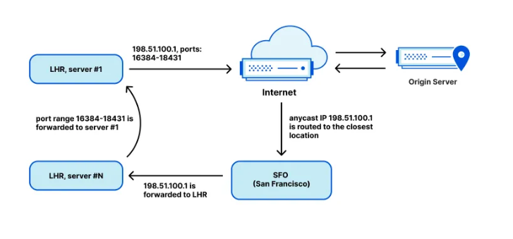
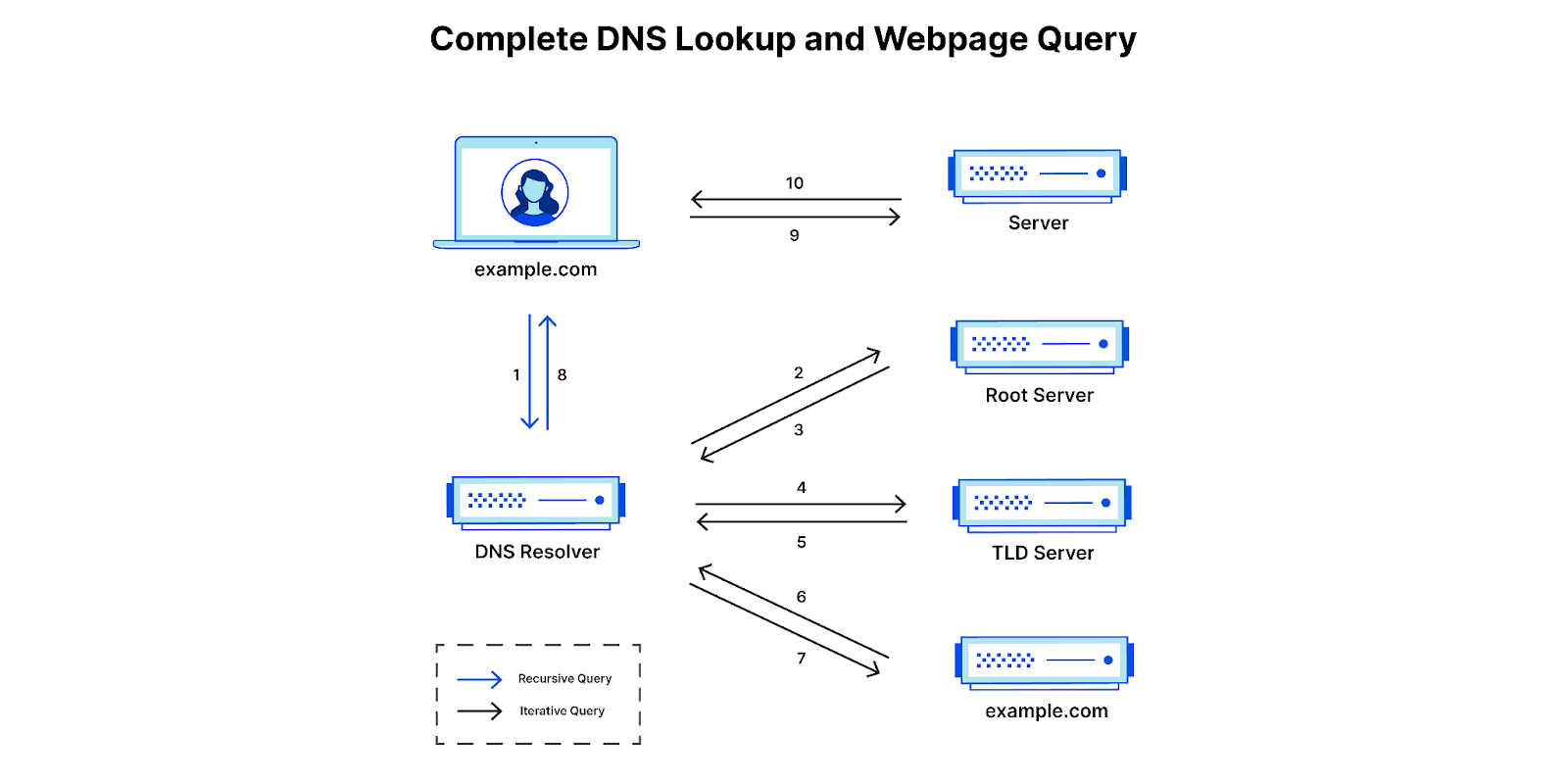
A quick refresher: Bring-your-own-IP is named for exactly what it does – it allows customers to bring their own IP space to Cloudflare. Customers choose BYOIP for a number of reasons, but the main reasons are control and configurability. An IP prefix is a range or block of IP addresses. Routers create a table of reachable prefixes, known as a routing table, to ensure that packets are delivered correctly across the Internet. When a customer’s Cloudflare services are configured to use the customer’s own addresses, onboarded to Cloudflare as BYOIP, a packet with a corresponding destination address will be routed across the Internet to Cloudflare’s global edge network, where it will be received and processed. BYOIP can be used with our Layer 7 services, Spectrum, or Magic Transit.
Let’s take a step back and take a look at the state of the BYOIP world right now. Let’s say a customer has authority over a range of IP addresses, and they’d like to bring them to Cloudflare. We require customers to provide us with a Letter of Authorization (LOA) and have an Internet Routing Registry (IRR) record matching their prefix and ASN. Once we have this, we require manual review by a Cloudflare engineer. There are a few issues with this process:
-
Insecure: The LOA is just a document—a piece of paper. The security of this method rests entirely on the diligence of the engineer reviewing the document. If the review is not able to detect that a document is fraudulent or inaccurate, it is possible for a prefix or ASN to be hijacked.
-
Time-consuming: Generating a single LOA is not always sufficient. If you are leasing IP space, we will ask you to provide documentation confirming that relationship as well, so that we can see a clear chain of authorisation from the original assignment or allocation of addresses to you. Getting all the paper documents to verify this chain of ownership, combined with having to wait for manual review can result in weeks of waiting to deploy a prefix!
Moving to a self-serve model allowed us to rethink the manner in which we conduct prefix ownership checks. We asked ourselves: How can we quickly, securely, and automatically prove you are authorized to use your IP prefix and intend to route it through Cloudflare?
We ended up killing two birds with one stone, thanks to our two-step process involving the creation of an RPKI ROA (verification of intent) and modification of IRR or rDNS records (verification of ownership). Self-serve unlocks the ability to not only onboard prefixes more quickly and without human intervention, but also exercises more rigorous ownership checks than a simple scanned document ever could. While not 100% foolproof, it is a significant improvement in the way we verify ownership.
Regional Internet Registries (RIRs) are the organizations responsible for distributing and managing Internet number resources like IP addresses. They are composed of 5 different entities operating in different regions of the world (RIRs). Originally allocated address space from the Internet Assigned Numbers Authority (IANA), they in turn assign and allocate that IP space to Local Internet Registries (LIRs) like ISPs.
This process is based on RIR policies which generally look at things like legal documentation, existing database/registry records, technical contacts, and BGP information. End-users can obtain addresses from an LIR, or in some cases through an RIR directly. As IPv4 addresses have become more scarce, brokerage services have been launched to allow addresses to be leased for fixed periods from their original assignees.
The Internet Routing Registry (IRR) is a separate system that focuses on routing rather than address assignment. Many organisations operate IRR instances and allow routing information to be published, including all five RIRs. While most IRR instances impose few barriers to the publication of routing data, those that are operated by RIRs are capable of linking the ability to publish routing information with the organisations to which the corresponding addresses have been assigned. We believe that being able to modify an IRR record protected in this way provides a good signal that a user has the rights to use a prefix.
Example of a route object containing validation token (using the documentation-only address 192.0.2.0/24):
% whois -h rr.arin.net 192.0.2.0/24

route:          192.0.2.0/24
origin:         AS13335
descr:          Example Company, Inc.
                cf-validation: 9477b6c3-4344-4ceb-85c4-6463e7d2453f
admin-c:        ADMIN2521-ARIN
tech-c:         ADMIN2521-ARIN
tech-c:         CLOUD146-ARIN
mnt-by:         MNT-CLOUD14
created:        2025-07-29T10:52:27Z
last-modified:  2025-07-29T10:52:27Z
source:         ARIN
For those that don’t want to go through the process of IRR-based validation, reverse DNS (rDNS) is provided as another secure method of verification. To manage rDNS for a prefix — whether it’s creating a PTR record or a security TXT record — you must be granted permission by the entity that allocated the IP block in the first place (usually your ISP or the RIR).
This permission is demonstrated in one of two ways:
-
Directly through the IP owner’s authenticated customer portal (ISP/RIR).
-
By the IP owner delegating authority to your third-party DNS provider via an NS record for your reverse zone.
Example of a reverse domain lookup using dig command (using the documentation-only address 192.0.2.0/24):
% dig cf-validation.2.0.192.in-addr.arpa TXT

; <<>> DiG 9.10.6 <<>> cf-validation.2.0.192.in-addr.arpa TXT
;; global options: +cmd
;; Got answer:
;; ->>HEADER<<- opcode: QUERY, status: NOERROR, id: 16686
;; flags: qr rd ra; QUERY: 1, ANSWER: 1, AUTHORITY: 0, ADDITIONAL: 1

;; OPT PSEUDOSECTION:
; EDNS: version: 0, flags:; udp: 4096
;; QUESTION SECTION:
;cf-validation.2.0.192.in-addr.arpa. IN TXT

;; ANSWER SECTION:
cf-validation.2.0.192.in-addr.arpa. 300 IN TXT "b2f8af96-d32d-4c46-a886-f97d925d7977"

;; Query time: 35 msec
;; SERVER: 127.0.2.2#53(127.0.2.2)
;; WHEN: Fri Oct 24 10:43:52 EDT 2025
;; MSG SIZE  rcvd: 150
So how exactly is one supposed to modify these records? That’s where the validation token comes into play. Once you choose either the IRR or Reverse DNS method, we provide a unique, single-use validation token. You must add this token to the content of the relevant record, either in the IRR or in the DNS. Our system then looks for the presence of the token as evidence that the request is being made by someone with authorization to make the requested modification. If the token is found, verification is complete and your ownership is confirmed!
Ownership is only half the battle; we also need to confirm your intention that you authorize Cloudflare to advertise your prefix. For this, we rely on the gold standard for routing security: the Resource Private Key Infrastructure (RPKI), and in particular Route Origin Authorization (ROA) objects.
A ROA is a cryptographically-signed document that specifies which Autonomous System Number (ASN) is authorized to originate your IP prefix. You can think of a ROA as the digital equivalent of a certified, signed, and notarised contract from the owner of the prefix.
Relying parties can validate the signatures in a ROA using the RPKI.You simply create a ROA that specifies Cloudflare’s ASN (AS13335) as an authorized originator and arrange for it to be signed. Many of our customers used hosted RPKI systems available through RIR portals for this. When our systems detect this signed authorization, your routing intention is instantly confirmed.
Many other companies that support BYOIP require a complex workflow involving creating self-signed certificates and manually modifying RDAP (Registration Data Access Protocol) records—a heavy administrative lift. By embracing a choice of IRR object modification and Reverse DNS TXT records, combined with RPKI, we offer a verification process that is much more familiar and straightforward for existing network operators.
While the new self-serve flow ditches the need for the “dinosaur relic” that is the LOA, many network operators around the world still rely on it as part of the process of accepting prefixes from other networks.
To help ensure your prefix is accepted by adjacent networks globally, Cloudflare automatically generates a document on your behalf to be distributed in place of a LOA. This document provides information about the checks that we have carried out to confirm that we are authorised to originate the customer prefix, and confirms the presence of valid ROAs to authorise our origination of it. In this way we are able to support the workflows of network operators we connect to who rely upon LOAs, without our customers having the burden of generating them.

One concern in designing the Self-Serve API is the trade-off between giving customers flexibility while implementing the necessary safeguards so that an IP prefix is never advertised without a matching service binding. If this were to happen, Cloudflare would be advertising a prefix with no idea on what to do with the traffic when we receive it! We call this “blackholing” traffic. To handle this, we introduced the requirement of a default service binding — i.e. a service binding that spans the entire range of the IP prefix onboarded.
A customer can later layer different service bindings on top of their default service binding via multiple service bindings, like putting CDN on top of a default Spectrum service binding. This way, a prefix can never be advertised without a service binding and blackhole our customers’ traffic.

Check out our developer docs on the most up-to-date documentation on how to onboard, advertise, and add services to your IP prefixes via our API. Remember that onboardings can be complex, and don’t hesitate to ask questions or reach out to our professional services team if you’d like us to do it for you.
The ability to script and integrate BYOIP management into existing workflows is a game-changer for modern network operations, and we’re only just getting started. In the months ahead, look for self-serve BYOIP in the dashboard, as well as self-serve BYOIP offboarding to give customers even more control.
Cloudflare’s self-serve BYOIP API onboarding empowers customers with unprecedented control and flexibility over their IP assets. This move to automate onboarding empowers a stronger security posture, moving away from manually-reviewed PDFs and driving RPKI adoption. By using these API calls, organizations can automate complex network tasks, streamline migrations, and build more resilient and agile network infrastructures.