Tag Archives: linux

So long, and thanks for all the fish: how to escape the Linux networking stack

Post Syndicated from Chris Branch original https://blog.cloudflare.com/so-long-and-thanks-for-all-the-fish-how-to-escape-the-linux-networking-stack/

There is a theory which states that if ever anyone discovers exactly what the Linux networking stack does and why it does it, it will instantly disappear and be replaced by something even more bizarre and inexplicable.

There is another theory which states that Git was created to track how many times this has already happened.

Many products at Cloudflare aren’t possible without pushing the limits of network hardware and software to deliver improved performance, increased efficiency, or novel capabilities such as soft-unicast, our method for sharing IP subnets across data centers. Happily, most people do not need to know the intricacies of how your operating system handles network and Internet access in general. Yes, even most people within Cloudflare.

But sometimes we try to push well beyond the design intentions of Linux’s networking stack. This is a story about one of those attempts.

Hard solutions for soft problems

My previous blog post about the Linux networking stack teased a problem matching the ideal model of soft-unicast with the basic reality of IP packet forwarding rules. Soft-unicast is the name given to our method of sharing IP addresses between machines. You may learn about all the cool things we do with it, but as far as a single machine is concerned, it has dozens to hundreds of combinations of IP address and source-port range, any of which may be chosen for use by outgoing connections.


The SNAT target in iptables supports a source-port range option to restrict the ports selected during NAT. In theory, we could continue to use iptables for this purpose, and to support multiple IP/port combinations we could use separate packet marks or multiple TUN devices. In actual deployment we would have to overcome challenges such as managing large numbers of iptables rules and possibly network devices, interference with other uses of packet marks, and deployment and reallocation of existing IP ranges.

Rather than increase the workload on our firewall, we wrote a single-purpose service dedicated to egressing IP packets on soft-unicast address space. For reasons lost in the mists of time, we named it SLATFATF, or “fish” for short. This service’s sole responsibility is to proxy IP packets using soft-unicast address space and manage the lease of those addresses.

WARP is not the only user of soft-unicast IP space in our network. Many Cloudflare products and services make use of the soft-unicast capability, and many of them use it in scenarios where we create a TCP socket in order to proxy or carry HTTP connections and other TCP-based protocols. Fish therefore needs to lease addresses that are not used by open sockets, and ensure that sockets cannot be opened to addresses leased by fish.

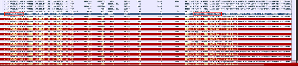
Our first attempt was to use distinct per-client addresses in fish and continue to let Netfilter/conntrack apply SNAT rules. However, we discovered an unfortunate interaction between Linux’s socket subsystem and the Netfilter conntrack module that reveals itself starkly when you use packet rewriting.

Collision avoidance

Suppose we have a soft-unicast address slice, 198.51.100.10:9000-9009. Then, suppose we have two separate processes that want to bind a TCP socket at 198.51.100.10:9000 and connect it to 203.0.113.1:443. The first process can do this successfully, but the second process will receive an error when it attempts to connect, because there is already a socket matching the requested 5-tuple.


Instead of creating sockets, what happens when we emit packets on a TUN device with the same destination IP but a unique source IP, and use source NAT to rewrite those packets to an address in this range?

If we add an nftables “snat” rule that rewrites the source address to 198.51.100.10:9000-9009, Netfilter will create an entry in the conntrack table for each new connection seen on fishtun, mapping the new source address to the original one. If we try to forward more connections on that TUN device to the same destination IP, new source ports will be selected in the requested range, until all ten available ports have been allocated; once this happens, new connections will be dropped until an existing connection expires, freeing an entry in the conntrack table.

Unlike when binding a socket, Netfilter will simply pick the first free space in the conntrack table. However, if you use up all the possible entries in the table you will get an EPERM error when writing an IP packet. Either way, whether you bind kernel sockets or you rewrite packets with conntrack, errors will indicate when there isn’t a free entry matching your requirements.

Now suppose that you combine the two approaches: a first process emits an IP packet on the TUN device that is rewritten to a packet on our soft-unicast port range. Then, a second process binds and connects a TCP socket with the same addresses as that IP packet:


The first problem is that there is no way for the second process to know that there is an active connection from 198.51.100.10:9000 to 203.0.113.1:443, at the time the connect() call is made. The second problem is that the connection is successful from the point of view of that second process.

It should not be possible for two connections to share the same 5-tuple. Indeed, they don’t. Instead, the source address of the TCP socket is silently rewritten to the next free port.


This behaviour is present even if you use conntrack without either SNAT or MASQUERADE rules. It usually happens that the lifetime of conntrack entries matches the lifetime of the sockets they’re related to, but this is not guaranteed, and you cannot depend on the source address of your socket matching the source address of the generated IP packets.

Crucially for soft-unicast, it means conntrack may rewrite our connection to have a source port outside of the port slice assigned to our machine. This will silently break the connection, causing unnecessary delays and false reports of connection timeouts. We need another solution.

Taking a breather

For WARP, the solution we chose was to stop rewriting and forwarding IP packets, instead to terminate all TCP connections within the server and proxy them to a locally-created TCP socket with the correct soft-unicast address. This was an easy and viable solution that we already employed for a portion of our connections, such as those directed at the CDN, or intercepted as part of the Zero Trust Secure Web Gateway. However, it does introduce additional resource usage and potentially increased latency compared to the status quo. We wanted to find another way (to) forward.

An inefficient interface

If you want to use both packet rewriting and bound sockets, you need to decide on a single source of truth. Netfilter is not aware of the socket subsystem, but most of the code that uses sockets and is also aware of soft-unicast is code that Cloudflare wrote and controls. A slightly younger version of myself therefore thought it made sense to change our code to work correctly in the face of Netfilter’s design.

Our first attempt was to use the Netlink interface to the conntrack module, to inspect and manipulate the connection tracking tables before sockets were created. Netlink is an extensible interface to various Linux subsystems and is used by many command-line tools like ip and, in our case, conntrack-tools. By creating the conntrack entry for the socket we are about to bind, we can guarantee that conntrack won’t rewrite the connection to an invalid port number, and ensure success every time. Likewise, if creating the entry fails, then we can try another valid address. This approach works regardless of whether we are binding a socket or forwarding IP packets.

There is one problem with this — it’s not terribly efficient. Netlink is slow compared to the bind/connect socket dance, and when creating conntrack entries you have to specify a timeout for the flow and delete the entry if your connection attempt fails, to ensure that the connection table doesn’t fill up too quickly for a given 5-tuple. In other words, you have to manually reimplement tcp_tw_reuse option to support high-traffic destinations with limited resources. In addition, a stray RST packet can erase your connection tracking entry. At our scale, anything like this that can happen, will happen. It is not a place for fragile solutions.

Socket to ‘em

Instead of creating conntrack entries, we can abuse kernel features for our own benefit. Some time ago Linux added the TCP_REPAIR socket option, ostensibly to support connection migration between servers e.g. to relocate a VM. The scope of this feature allows you to create a new TCP socket and specify its entire connection state by hand.

An alternative use of this is to create a “connected” socket that never performed the TCP three-way handshake needed to establish that connection. At least, the kernel didn’t do that — if you are forwarding the IP packet containing a TCP SYN, you have more certainty about the expected state of the world.

However, the introduction of TCP Fast Open provides an even simpler way to do this: you can create a “connected” socket that doesn’t perform the traditional three-way handshake, on the assumption that the SYN packet — when sent with its initial payload — contains a valid cookie to immediately establish the connection. However, as nothing is sent until you write to the socket, this serves our needs perfectly.

You can try this yourself:

TCP_FASTOPEN_CONNECT = 30
TCP_FASTOPEN_NO_COOKIE = 34
s = socket(AF_INET, SOCK_STREAM)
s.setsockopt(SOL_TCP, TCP_FASTOPEN_CONNECT, 1)
s.setsockopt(SOL_TCP, TCP_FASTOPEN_NO_COOKIE, 1)
s.bind(('198.51.100.10', 9000))
s.connect(('1.1.1.1', 53))

Binding a “connected” socket that nevertheless corresponds to no actual socket has one important feature: if other processes attempt to bind to the same addresses as the socket, they will fail to do so. This satisfies the problem we had at the beginning to make packet forwarding coexist with socket usage.

Jumping the queue

While this solves one problem, it creates another. By default, you can’t use an IP address for both locally-originated packets and forwarded packets.

For example, we assign the IP address 198.51.100.10 to a TUN device. This allows any program to create a TCP socket using the address 198.51.100.10:9000. We can also write packets to that TUN device with the address 198.51.100.10:9001, and Linux can be configured to forward those packets to a gateway, following the same route as the TCP socket. So far, so good.

On the inbound path, TCP packets addressed to 198.51.100.10:9000 will be accepted and data put into the TCP socket. TCP packets addressed to 198.51.100.10:9001, however, will be dropped. They are not forwarded to the TUN device at all.

Why is this the case? Local routing is special. If packets are received to a local address, they are treated as “input” and not forwarded, regardless of any routing you think should apply. Behold the default routing rules:

cbranch@linux:~$ ip rule
0:        from all lookup local
32766:    from all lookup main
32767:    from all lookup default

The rule priority is a nonnegative integer, the smallest priority value is evaluated first. This requires some slightly awkward rule manipulation to “insert” a lookup rule at the beginning that redirects marked packets to the packet forwarding service’s TUN device; you have to delete the existing rule, then create new rules in the right order. However, you don’t want to leave the routing rules without any route to the “local” table, in case you lose a packet while manipulating these rules. In the end, the result looks something like this:

ip rule add fwmark 42 table 100 priority 10
ip rule add lookup local priority 11
ip rule del priority 0
ip route add 0.0.0.0/0 proto static dev fishtun table 100

As with WARP, we simplify connection management by assigning a mark to packets coming from the “fishtun” interface, which we can use to route them back there. To prevent locally-originated TCP sockets from having this same mark applied, we assign the IP to the loopback interface instead of fishtun, leaving fishtun with no assigned address. But it doesn’t need one, as we have explicit routing rules now.

Uncharted territory

While testing this last fix, I ran into an unfortunate problem. It did not work in our production environment.

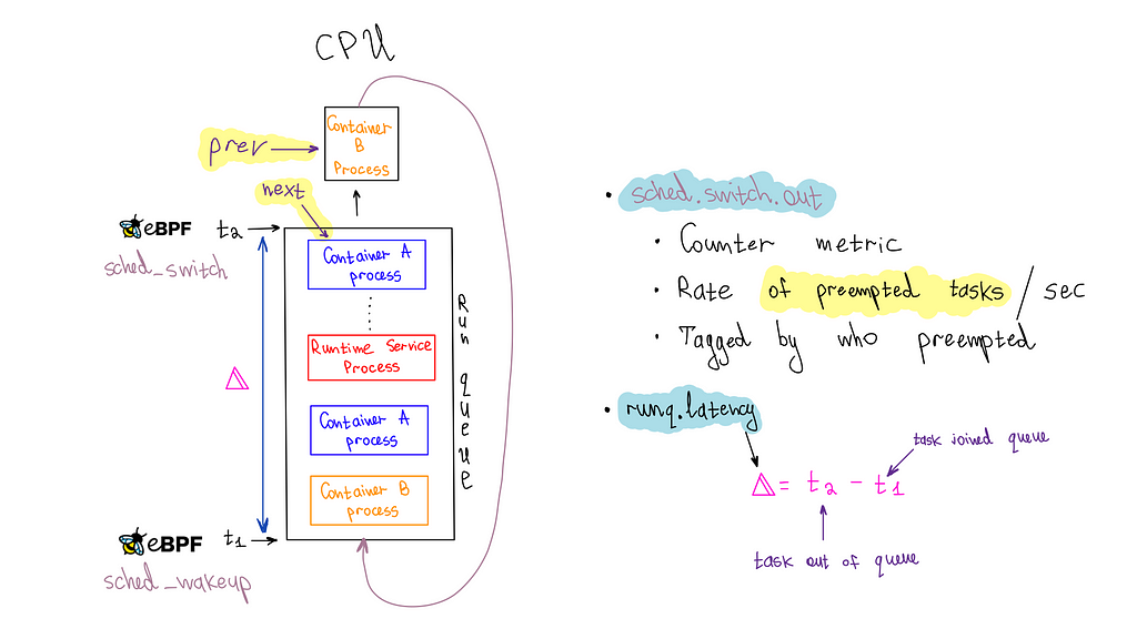
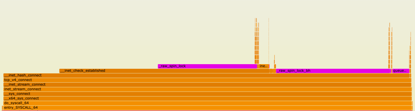
It is not simple to debug the path of a packet through Linux’s networking stack. There are a few tools you can use, such as setting nftrace in nftables or applying the LOG/TRACE targets in iptables, which help you understand which rules and tables are applied for a given packet.


Schematic for the packet flow paths through Linux networking and *tables by Jan Engelhardt

Our expectation is that the packet will pass the prerouting hook, a routing decision is made to send the packet to our TUN device, then the packet will traverse the forward table. By tracing packets originating from the IP of a test host, we could see the packets enter the prerouting phase, but disappear after the ‘routing decision’ block.

While there is a block in the diagram for “socket lookup”, this occurs after processing the input table. Our packet doesn’t ever enter the input table; the only change we made was to create a local socket. If we stop creating the socket, the packet passes to the forward table as before.

It turns out that part of the ‘routing decision’ involves some protocol-specific processing. For IP packets, routing decisions can be cached, and some basic address validation is performed. In 2012, an additional feature was added: early demux. The rationale being, at this point in packet processing we are already looking up something, and the majority of packets received are expected to be for local sockets, rather than an unknown packet or one that needs to be forwarded somewhere. In this case, why not look up the socket directly here and save yourself an extra route lookup?

The workaround at the end of the universe

Unfortunately for us, we just created a socket and didn’t want it to receive packets. Our adjustment to the routing table is ignored, because that routing lookup is skipped entirely when the socket is found. Raw sockets avoid this by receiving all packets regardless of the routing decision, but the packet rate is too high for this to be efficient. The only way around this is disabling the early demux feature. According to the patch’s claims, though, this feature improves performance: how far will performance regress on our existing workloads if we disable it?

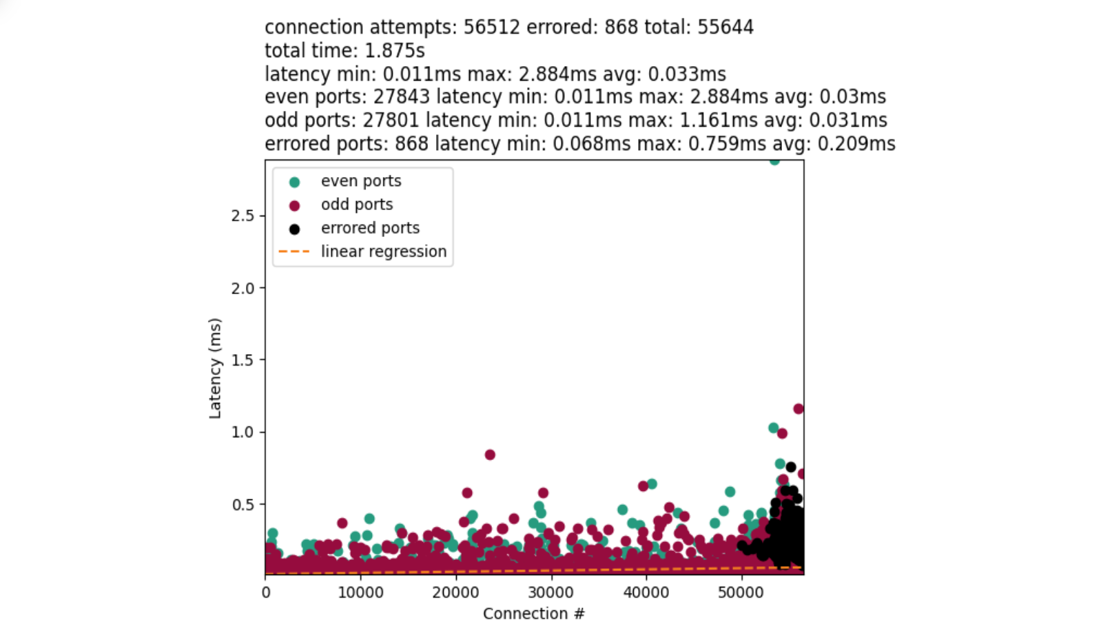
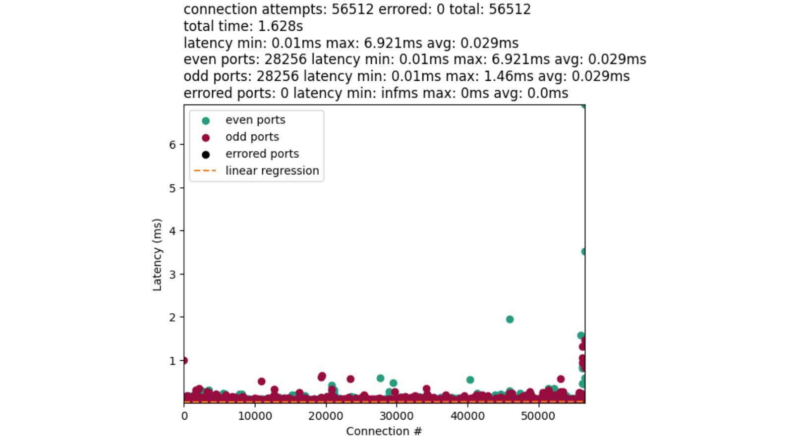
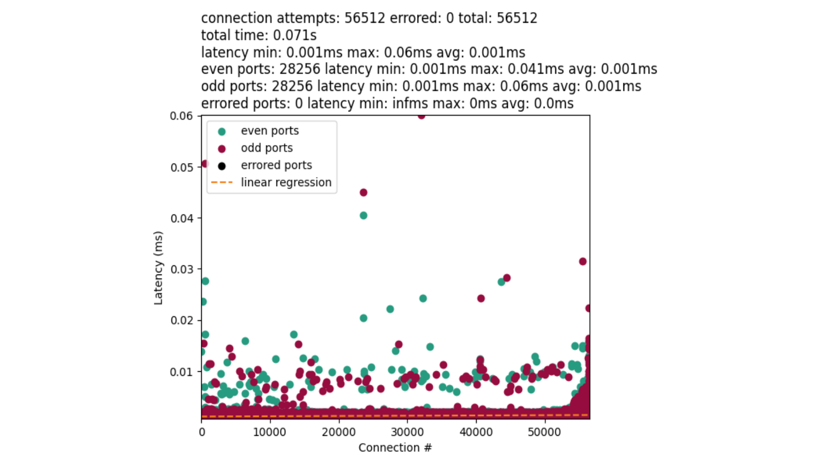
This calls for a simple experiment: set the net.ipv4.tcp_early_demux syscall to 0 on some machines in a datacenter, let it run for a while, then compare the CPU usage with machines using default settings and the same hardware configuration as the machines under test.


The key metrics are CPU usage from /proc/stat. If there is a performance degradation, we would expect to see higher CPU usage allocated to “softirq” — the context in which Linux network processing occurs — with little change to either userspace (top) or kernel time (bottom). The observed difference is slight, and mostly appears to reduce efficiency during off-peak hours.

Swimming upstream

While we tested different solutions to IP packet forwarding, we continued to terminate TCP connections on our network. Despite our initial concerns, the performance impact was small, and the benefits of increased visibility into origin reachability, fast internal routing within our network, and simpler observability of soft-unicast address usage flipped the burden of proof: was it worth trying to implement pure IP forwarding and supporting two different layers of egress?

So far, the answer is no. Fish runs on our network today, but with the much smaller responsibility of handling ICMP packets. However, when we decide to tunnel all IP packets, we know exactly how to do it.

A typical engineering role at Cloudflare involves solving many strange and difficult problems at scale. If you are the kind of goal-focused engineer willing to try novel approaches and explore the capabilities of the Linux kernel despite minimal documentation, look at our open positions — we would love to hear from you!

How to build your own VPN, or: the history of WARP

Post Syndicated from Chris Branch original https://blog.cloudflare.com/how-to-build-your-own-vpn-or-the-history-of-warp/

Linux’s networking capabilities are a crucial part of how Cloudflare serves billions of requests in the face of DDoS attacks. The tools it provides us are invaluable and useful, and a constant stream of contributions from developers worldwide ensures it continually gets more capable and performant.

When we developed WARP, our mobile-first performance and security app, we faced a new challenge: how to securely and efficiently egress arbitrary user packets for millions of mobile clients from our edge machines. This post explores our first solution, which was essentially building our own high-performance VPN with the Linux networking stack. We needed to integrate it into our existing network; not just directly linking it into our CDN service, but providing a way to securely egress arbitrary user packets from Cloudflare machines. The lessons we learned here helped us develop new products and capabilities and discover more strange things besides. But first, how did we get started?

A bridge between two worlds

WARP’s initial implementation resembled a virtual private network (VPN) that allows Internet access through it. Specifically, a Layer 3 VPN – a tunnel for IP packets.

IP packets are the building blocks of the Internet. When you send data over the Internet, it is split into small chunks and sent separately in packets, each one labeled with a destination address (who the packet goes to) and a source address (who to send a reply to). If you are connected to the Internet, you have an IP address.

You may not have a unique IP address, though. This is certainly true for IPv4 which, despite our and many others’ long-standing efforts to move everyone to IPv6, is still in widespread use. IPv4 has only 4 billion possible addresses and they have all been assigned – you’re gonna have to share.

When you use WiFi at home, work or the coffee shop, you’re connected to a local network. Your device is assigned a local IP address to talk to the access point and any other devices in your network. However, that address has no meaning outside of the local network. You can’t use that address in IP packets sent over the Internet, because every local IPv4 network uses the same few sets of addresses.

So how does Internet access work? Local IPv4 networks generally employ a router, a device to perform network-address translation (NAT). NAT is used to convert the private IPv4 network addresses allocated to devices on the local-area network to a small set of publicly-routable addresses given by your Internet service provider. The router keeps track of the conversions it applies between the two networks in a translation table. When a packet is received on either network, the router consults the translation table and applies the appropriate conversion before sending the packet to the opposite network.


Diagram of a router using NAT to bridge connections from devices on a private network to the public Internet

A VPN that provides Internet access is no different in this respect to a LAN – the only unusual aspect is that the user of the VPN communicates with the VPN server over the public Internet. The model is simple: private network IP packets are tunnelled, or encapsulated, in public IP packets addressed to the VPN server.


Schematic of HTTPS packets being encapsulated between a VPN client and server

Most times, VPN software only handles the encapsulation and decapsulation of packets, and gives you a virtual network device to send and receive packets on the VPN. This gives you the freedom to configure the VPN however you like. For WARP, we need our servers to act as a router between the VPN client and the Internet.

NAT’s how you do it

Linux – the operating system powering our servers – can be configured to perform routing with NAT in its Netfilter subsystem. Netfilter is frequently configured through nftables or iptables rules. Configuring a “source NAT” to rewrite the source IP of outgoing packets is achieved with a single rule:

nft add rule ip nat postrouting oifname "eth0" ip saddr 10.0.0.0/8 snat to 198.51.100.42

This rule configures Netfilter’s NAT feature to perform source address translation for any packet matching the following criteria:

  1. The source address is the 10.0.0.0/8 private network subnet – in this example, let’s say VPN clients have addresses from this subnet.

  2. The packet shall be sent on the “eth0” interface – in this example, it’s the server’s only physical network interface, and thus the route to the public Internet.

Where these two conditions are true, we apply the “snat” action to rewrite the source IP packet, from whichever address the VPN client is using, to our example server’s public IP address 198.51.100.42. We keep track of the original and rewritten addresses in the rewrite table.


Schematic of an encapsulated packet being decapsulated and rewritten by a VPN server

You may require additional configuration depending on how your distribution ships nftables – nftables is more flexible than the deprecated iptables, but has fewer “implicit” tables ready to use.

You also might need to enable IP forwarding in general, as by default you don’t want a machine connected to two different networks to forward between them without realising it.

A conntrack is a conntrack is a conntrack

We said before that a router keeps track of the conversions between addresses in the two networks. In the diagram above, that state is held in the rewrite table.

In practice, any device may only implement NAT usefully if it understands the TCP and UDP protocols, in particular how they use port numbers to support multiple independent flows of data on a single IP address. The NAT device – in our case Linux – ensures that a unique source port and address is used for each connection, and reassigns the port if required. It also needs to understand the lifecycle of a TCP connection, so that it knows when it is safe to reuse a port number: with only 65,536 possible ports, port reuse is essential.

Linux Netfilter has the conntrack module, widely used to implement a stateful firewall that protects servers against spoofed or unexpected packets, preventing them interfering with legitimate connections. This protection is possible because it understands TCP and the valid state of a connection. This capability means it’s perfectly positioned to implement NAT, too. In fact, all packet rewriting is implemented by conntrack.


A diagram showing the steps taken by conntrack to validate and rewrite packets

As a stateful firewall, the conntrack module maintains a table of all connections it has seen. If you know all of the active connections, you can rewrite a new connection to a port that is not in use.

In the “snat” rule above, Netfilter adds an entry to the rewrite table, but doesn’t change the packet yet. Only basic packet changes are permitted within nftables. We must wait for packet processing to reach the conntrack module, which selects a port unused by any active connection, and only then rewrites the packet.


A diagram showing the roles of netfilter and conntrack when applying NAT to traffic

Marky mark and the firewall bunch

Another mode of conntrack is to assign a persistent mark to packets belonging to a connection. The mark can be referenced in nftables rules to implement different firewall policies, or to control routing decisions.

Suppose you want to prevent specific addresses (e.g. from a guest network) from accessing certain services on your machine. You could add a firewall rule for each service denying access to those addresses. However, if you need to change the set of addresses to block, you have to update every rule accordingly.

Alternatively, you could use one rule to apply a mark to packets coming from the addresses you wish to block, and then reference the mark in all the service rules that implement the block. Now if you wish to change the addresses, you need only update a single rule to change the scope of that packet mark.

This is most beneficial to control routing behaviour, as routing rules cannot make decisions on as many attributes of the packet as Netfilter can. Using marks allows you to select packets based on powerful Netfilter rules.


A diagram showing netfilter marking specific packets to apply special routing rules

The code powering the WARP service was written by Cloudflare in Rust, a security-focused systems programming language. We took great care implementing boringtun – our WireGuard implementation – and MASQUE. But even if you think the front door is impenetrable, it is good security practice to employ defense-in-depth.

One example is distinguishing IP packets that come from clients vs. packets that originate elsewhere in our network. One common method is to allocate a unique IP space to WARP traffic and distinguish it based on IP address, but this can be fragile if we need to apply a configuration change to renumber our internal networks – remember IPv4’s limited address space! Instead we can do something simpler.

To bring IP packets from WARP clients into the Linux networking stack, WARP uses a TUN device – Linux’s name for the virtual network device that programs can use to send and receive IP packets. A TUN device can be configured similarly to any other network device like Ethernet or Wi-Fi adapters, including firewall and routing.

Using nftables, we mark all packets output on WARP’s TUN device. We have to explicitly store the mark in conntrack’s state table on the outgoing path and retrieve it for the incoming packet, as netfilter can use packet marks independently of conntrack.

table ip mangle {
    chain forward {
        type filter hook forward priority mangle; policy accept;
        oifname "fishtun" counter ct mark set 42
    }
    chain prerouting {
        type filter hook prerouting priority mangle; policy accept;
        counter meta mark set ct mark
    }
}

We also need to add a routing rule to return marked packets to the TUN device:

ip rule add fwmark 42 table 100 priority 10
ip route add 0.0.0.0/0 proto static dev warp-tun table 100

Now we’re done. All connections from WARP are clearly identified and can be firewalled separately from locally-originated connections or other nodes on our network. Conntrack handles NAT for us, and the connection marks tell us which tracked connections were made by WARP clients.

The end?

In our first version of WARP, we enabled clients to access arbitrary Internet hosts by combining multiple components of Linux’s networking stack. Each of our edge servers had a single IP address from an allocation dedicated to WARP, and we were able to configure NAT, routing, and appropriate firewall rules using standard and well-documented methods.

Linux is flexible and easy to configure, but it would require one IPv4 address per machine. Due to IPv4 address exhaustion, this approach would not scale to Cloudflare’s large network. Assigning a dedicated IPv4 address for every machine that runs the WARP server results in an eye-watering address lease bill. To bring costs down, we would have to limit the number of servers running WARP, increasing the operational complexity of deploying it.

We had ideas, but we would have to give up the easy path Linux gave us. IP sharing seemed to us the most promising solution, but how much has to change if a single machine can only receive packets addressed to a narrow set of ports? We will reveal all in a follow-up blog post, but if you are the kind of curious problem-solving engineer who is already trying to imagine solutions to this problem, look at our open positions – we’d like to hear from you!

A deep dive into BPF LPM trie performance and optimization

Post Syndicated from Matt Fleming original https://blog.cloudflare.com/a-deep-dive-into-bpf-lpm-trie-performance-and-optimization/

It started with a mysterious soft lockup message in production. A single, cryptic line that led us down a rabbit hole into the performance of one of the most fundamental data structures we use: the BPF LPM trie.

BPF trie maps (BPF_MAP_TYPE_LPM_TRIE) are heavily used for things like IP and IP+Port matching when routing network packets, ensuring your request passes through the right services before returning a result. The performance of this data structure is critical for serving our customers, but the speed of the current implementation leaves a lot to be desired. We’ve run into several bottlenecks when storing millions of entries in BPF LPM trie maps, such as entry lookup times taking hundreds of milliseconds to complete and freeing maps locking up a CPU for over 10 seconds. For instance, BPF maps are used when evaluating Cloudflare’s Magic Firewall rules and these bottlenecks have even led to traffic packet loss for some customers.

This post gives a refresher of how tries and prefix matching work, benchmark results, and a list of the shortcomings of the current BPF LPM trie implementation.

A brief recap of tries

If it’s been a while since you last looked at the trie data structure (or if you’ve never seen it before), a trie is a tree data structure (similar to a binary tree) that allows you to store and search for data for a given key and where each node stores some number of key bits.

Searches are performed by traversing a path, which essentially reconstructs the key from the traversal path, meaning nodes do not need to store their full key. This differs from a traditional binary search tree (BST) where the primary invariant is that the left child node has a key that is less than the current node and the right child has a key that is greater. BSTs require that each node store the full key so that a comparison can be made at each search step.

Here’s an example that shows how a BST might store values for the keys:

  • ABC

  • ABCD

  • ABCDEFGH

  • DEF


In comparison, a trie for storing the same set of keys might look like this.


This way of splitting out bits is really memory-efficient when you have redundancy in your data, e.g. prefixes are common in your keys, because that shared data only requires a single set of nodes. It’s for this reason that tries are often used to efficiently store strings, e.g. dictionaries of words – storing the strings “ABC” and “ABCD” doesn’t require 3 bytes + 4 bytes (assuming ASCII), it only requires 3 bytes + 1 byte because “ABC” is shared by both (the exact number of bits required in the trie is implementation dependent).

Tries also allow more efficient searching. For instance, if you wanted to know whether the key “CAR” existed in the BST you are required to go to the right child of the root (the node with key “DEF”) and check its left child because this is where it would live if it existed. A trie is more efficient because it searches in prefix order. In this particular example, a trie knows at the root whether that key is in the trie or not.

This design makes tries perfectly suited for performing longest prefix matches and for working with IP routing using CIDR. CIDR was introduced to make more efficient use of the IP address space (no longer requiring that classes fall into 4 buckets of 8 bits) but comes with added complexity because now the network portion of an IP address can fall anywhere. Handling the CIDR scheme in IP routing tables requires matching on the longest (most specific) prefix in the table rather than performing a search for an exact match.

If searching a trie does a single-bit comparison at each node, that’s a binary trie. If searching compares more bits we call that a multibit trie. You can store anything you like in a trie, including IP and subnet addresses – it’s all just ones and zeroes.

Nodes in multibit tries use more memory than in binary tries, but since computers operate on multibit words anyhow, it’s more efficient from a microarchitecture perspective to use multibit tries because you can traverse through the bits faster, reducing the number of comparisons you need to make to search for your data. It’s a classic space vs time tradeoff.

There are other optimisations we can use with tries. The distribution of data that you store in a trie might not be uniform and there could be sparsely populated areas. For example, if you store the strings “A” and “BCDEFGHI” in a multibit trie, how many nodes do you expect to use? If you’re using ASCII, you could construct the binary trie with a root node and branch left for “A” or right for “B”. With 8-bit nodes, you’d need another 7 nodes to store “C”, “D”, “E”, “F”, “G”, “H”, “I”.


Since there are no other strings in the trie, that’s pretty suboptimal. Once you hit the first level after matching on “B” you know there’s only one string in the trie with that prefix, and you can avoid creating all the other nodes by using path compression. Path compression replaces nodes “C”, “D”, “E” etc. with a single one such as “I”.


If you traverse the tree and hit “I”, you still need to compare the search key with the bits you skipped (“CDEFGH”) to make sure your search key matches the string. Exactly how and where you store the skipped bits is implementation dependent – BPF LPM tries simply store the entire key in the leaf node. As your data becomes denser, path compression is less effective.

What if your data distribution is dense and, say, all the first 3 levels in a trie are fully populated? In that case you can use level compression and replace all the nodes in those levels with a single node that has 2**3 children. This is how Level-Compressed Tries work which are used for IP route lookup in the Linux kernel (see net/ipv4/fib_trie.c).

There are other optimisations too, but this brief detour is sufficient for this post because the BPF LPM trie implementation in the kernel doesn’t fully use the three we just discussed.

How fast are BPF LPM trie maps?

Here are some numbers from running BPF selftests benchmark on AMD EPYC 9684X 96-Core machines. Here the trie has 10K entries, a 32-bit prefix length, and an entry for every key in the range [0, 10K).

Operation

Throughput

Stddev

Latency

lookup

7.423M ops/s

0.023M ops/s

134.710 ns/op

update

2.643M ops/s

0.015M ops/s

378.310 ns/op

delete

0.712M ops/s

0.008M ops/s

1405.152 ns/op

free

0.573K ops/s

0.574K ops/s

1.743 ms/op

The time to free a BPF LPM trie with 10K entries is noticeably large. We recently ran into an issue where this took so long that it caused soft lockup messages to spew in production.

This benchmark gives some idea of worst case behaviour. Since the keys are so densely populated, path compression is completely ineffective. In the next section, we explore the lookup operation to understand the bottlenecks involved.

Why are BPF LPM tries slow?

The LPM trie implementation in kernel/bpf/lpm_trie.c has a couple of the optimisations we discussed in the introduction. It is capable of multibit comparisons at leaf nodes, but since there are only two child pointers in each internal node, if your tree is densely populated with a lot of data that only differs by one bit, these multibit comparisons degrade into single bit comparisons.

Here’s an example. Suppose you store the numbers 0, 1, and 3 in a BPF LPM trie. You might hope that since these values fit in a single 32 or 64-bit machine word, you could use a single comparison to decide which next node to visit in the trie. But that’s only possible if your trie implementation has 3 child pointers in the current node (which, to be fair, most trie implementations do). In other words, you want to make a 3-way branching decision but since BPF LPM tries only have two children, you’re limited to a 2-way branch.

A diagram for this 2-child trie is given below.


The leaf nodes are shown in green with the key, as a binary string, in the center. Even though a single 8-bit comparison is more than capable of figuring out which node has that key, the BPF LPM trie implementation resorts to inserting intermediate nodes (blue) to inject 2-way branching decisions into your path traversal because its parent (the orange root node in this case) only has 2 children. Once you reach a leaf node, BPF LPM tries can perform a multibit comparison to check the key. If a node supported pointers to more children, the above trie could instead look like this, allowing a 3-way branch and reducing the lookup time.


This 2-child design impacts the height of the trie. In the worst case, a completely full trie essentially becomes a binary search tree with height log2(nr_entries) and the height of the trie impacts how many comparisons are required to search for a key.

The above trie also shows how BPF LPM tries implement a form of path compression – you only need to insert an intermediate node where you have two nodes whose keys differ by a single bit. If instead of 3, you insert a key of 15 (0b1111), this won’t change the layout of the trie; you still only need a single node at the right child of the root.


And finally, BPF LPM tries do not implement level compression. Again, this stems from the fact that nodes in the trie can only have 2 children. IP route tables tend to have many prefixes in common and you typically see densely packed tries at the upper levels which makes level compression very effective for tries containing IP routes.

Here’s a graph showing how the lookup throughput for LPM tries (measured in million ops/sec) degrades as the number of entries increases, from 1 entry up to 100K entries.


Once you reach 1 million entries, throughput is around 1.5 million ops/sec, and continues to fall as the number of entries increases.


Why is this? Initially, this is because of the L1 dcache miss rate. All of those nodes that need to be traversed in the trie are potential cache miss opportunities.


As you can see from the graph, L1 dcache miss rate remains relatively steady and yet the throughput continues to decline. At around 80K entries, dTLB miss rate becomes the bottleneck.


Because BPF LPM tries to dynamically allocate individual nodes from a freelist of kernel memory, these nodes can live at arbitrary addresses. Which means traversing a path through a trie almost certainly will incur cache misses and potentially dTLB misses. This gets worse as the number of entries, and height of the trie, increases.


Where do we go from here?

By understanding the current limitations of the BPF LPM trie, we can now work towards building a more performant and efficient solution for the future of the Internet.

We’ve already contributed these benchmarks to the upstream Linux kernel — but that’s only the start. We have plans to improve the performance of BPM LPM tries, particularly the lookup function which is heavily used for our workloads. This post covered a number of optimisations that are already used by the net/ipv4/fib_trie.c code, so a natural first step is to refactor that code so that a common Level Compressed trie implementation can be used. Expect future blog posts to explore this work in depth.

If you’re interested in looking at more performance numbers, Jesper Brouer has recorded some here: https://github.com/xdp-project/xdp-project/blob/main/areas/bench/bench02_lpm-trie-lookup.org.

If the Linux kernel, performance, or optimising data structures excites you, our engineering teams are hiring.

Safe in the sandbox: security hardening for Cloudflare Workers

Post Syndicated from Erik Corry original https://blog.cloudflare.com/safe-in-the-sandbox-security-hardening-for-cloudflare-workers/

As a serverless cloud provider, we run your code on our globally distributed infrastructure. Being able to run customer code on our network means that anyone can take advantage of our global presence and low latency. Workers isn’t just efficient though, we also make it simple for our users. In short: You write code. We handle the rest.

Part of ‘handling the rest’ is making Workers as secure as possible. We have previously written about our security architecture. Making Workers secure is an interesting problem because the whole point of Workers is that we are running third party code on our hardware. This is one of the hardest security problems there is: any attacker has the full power available of a programming language running on the victim’s system when they are crafting their attacks.

This is why we are constantly updating and improving the Workers Runtime to take advantage of the latest improvements in both hardware and software. This post shares some of the latest work we have been doing to keep Workers secure.

Some background first: Workers is built around the V8 JavaScript runtime, originally developed for Chromium-based browsers like Chrome. This gives us a head start, because V8 was forged in an adversarial environment, where it has always been under intense attack and scrutiny. Like Workers, Chromium is built to run adversarial code safely. That’s why V8 is constantly being tested against the best fuzzers and sanitizers, and over the years, it has been hardened with new technologies like Oilpan/cppgc and improved static analysis.

We use V8 in a slightly different way, though, so we will be describing in this post how we have been making some changes to V8 to improve security in our use case.

Hardware-assisted security improvements from Memory Protection Keys

Modern CPUs from Intel, AMD, and ARM have support for memory protection keys, sometimes called PKU, Protection Keys for Userspace. This is a great security feature which increases the power of virtual memory and memory protection.

Traditionally, the memory protection features of the CPU in your PC or phone were mainly used to protect the kernel and to protect different processes from each other. Within each process, all threads had access to the same memory. Memory protection keys allow us to prevent specific threads from accessing memory regions they shouldn’t have access to.

V8 already uses memory protection keys for the JIT compilers. The JIT compilers for a language like JavaScript generate optimized, specialized versions of your code as it runs. Typically, the compiler is running on its own thread, and needs to be able to write data to the code area in order to install its optimized code. However, the compiler thread doesn’t need to be able to run this code. The regular execution thread, on the other hand, needs to be able to run, but not modify, the optimized code. Memory protection keys offer a way to give each thread the permissions it needs, but no more. And the V8 team in the Chromium project certainly aren’t standing still. They describe some of their future plans for memory protection keys here.

In Workers, we have some different requirements than Chromium. The security architecture for Workers uses V8 isolates to separate different scripts that are running on our servers. (In addition, we have extra mitigations to harden the system against Spectre attacks). If V8 is working as intended, this should be enough, but we believe in defense in depth: multiple, overlapping layers of security controls.

That’s why we have deployed internal modifications to V8 to use memory protection keys to isolate the isolates from each other. There are up to 15 different keys available on a modern x64 CPU and a few are used for other purposes in V8, so we have about 12 to work with. We give each isolate a random key which is used to protect its V8 heap data, the memory area containing the JavaScript objects a script creates as it runs. This means security bugs that might previously have allowed an attacker to read data from a different isolate would now hit a hardware trap in 92% of cases. (Assuming 12 keys, 92% is about 11/12.)


The illustration shows an attacker attempting to read from a different isolate. Most of the time this is detected by the mismatched memory protection key, which kills their script and notifies us, so we can investigate and remediate. The red arrow represents the case where the attacker got lucky by hitting an isolate with the same memory protection key, represented by the isolates having the same colors.

However, we can further improve on a 92% protection rate. In the last part of this blog post we’ll explain how we can lift that to 100% for a particular common scenario. But first, let’s look at a software hardening feature in V8 that we are taking advantage of.

The V8 sandbox, a software-based security boundary

Over the past few years, V8 has been gaining another defense in depth feature: the V8 sandbox. (Not to be confused with the layer 2 sandbox which Workers have been using since the beginning.) The V8 sandbox has been a multi-year project that has been gaining maturity for a while. The sandbox project stems from the observation that many V8 security vulnerabilities start by corrupting objects in the V8 heap memory. Attackers then leverage this corruption to reach other parts of the process, giving them the opportunity to escalate and gain more access to the victim’s browser, or even the entire system.

V8’s sandbox project is an ambitious software security mitigation that aims to thwart that escalation: to make it impossible for the attacker to progress from a corruption on the V8 heap to a compromise of the rest of the process. This means, among other things, removing all pointers from the heap. But first, let’s explain in as simple terms as possible, what a memory corruption attack is.

Memory corruption attacks

A memory corruption attack tricks a program into misusing its own memory. Computer memory is just a store of integers, where each integer is stored in a location. The locations each have an address, which is also just a number. Programs interpret the data in these locations in different ways, such as text, pixels, or pointers. Pointers are addresses that identify a different memory location, so they act as a sort of arrow that points to some other piece of data.

Here’s a concrete example, which uses a buffer overflow. This is a form of attack that was historically common and relatively simple to understand: Imagine a program has a small buffer (like a 16-character text field) followed immediately by an 8-byte pointer to some ordinary data. An attacker might send the program a 24-character string, causing a “buffer overflow.” Because of a vulnerability in the program, the first 16 characters fill the intended buffer, but the remaining 8 characters spill over and overwrite the adjacent pointer.


See below for how such an attack would now be thwarted.

Now the pointer has been redirected to point at sensitive data of the attacker’s choosing, rather than the normal data it was originally meant to access. When the program tries to use what it believes is its normal pointer, it’s actually accessing sensitive data chosen by the attacker.

This type of attack works in steps: first create a small confusion (like the buffer overflow), then use that confusion to create bigger problems, eventually gaining access to data or capabilities the attacker shouldn’t have.  The attacker can eventually use the misdirection to either steal information or plant malicious data that the program will treat as legitimate.

This was a somewhat abstract description of memory corruption attacks using a buffer overflow, one of the simpler techniques. For some much more detailed and recent examples, see this description from Google, or this breakdown of a V8 vulnerability.

Compressed pointers in V8

Many attacks are based on corrupting pointers, so ideally we would remove all pointers from the memory of the program.  Since an object-oriented language’s heap is absolutely full of pointers, that would seem, on its face, to be a hopeless task, but it is enabled by an earlier development. Starting in 2020, V8 has offered the option of saving memory by using compressed pointers. This means that, on a 64-bit system, the heap uses only 32 bit offsets, relative to a base address. This limits the total heap to maximally 4 GiB, a limitation that is acceptable for a browser, and also fine for individual scripts running in a V8 isolate on Cloudflare Workers.


An artificial object with various fields, showing how the layout differs in a compressed vs. an uncompressed heap. The boxes are 64 bits wide.

If the whole of the heap is in a single 4 GiB area then the first 32 bits of all pointers will be the same, and we don’t need to store them in every pointer field in every object. In the diagram we can see that the object pointers all start with 0x12345678, which is therefore redundant and doesn’t need to be stored. This means that object pointer fields and integer fields can be reduced from 64 to 32 bits.

We still need 64 bit fields for some fields like double precision floats and for the sandbox offsets of buffers, which are typically used by the script for input and output data. See below for details.

Integers in an uncompressed heap are stored in the high 32 bits of a 64 bit field. In the compressed heap, the top 31 bits of a 32 bit field are used. In both cases the lowest bit is set to 0 to indicate integers (as opposed to pointers or offsets).

Conceptually, we have two methods for compressing and decompressing, using a base address that is divisible by 4 GiB:

// Decompress a 32 bit offset to a 64 bit pointer by adding a base address.
void* Decompress(uint32_t offset) { return base + offset; }
// Compress a 64 bit pointer to a 32 bit offset by discarding the high bits.
uint32_t Compress(void* pointer) { return (intptr_t)pointer & 0xffffffff; }

This pointer compression feature, originally primarily designed to save memory, can be used as the basis of a sandbox.

From compressed pointers to the sandbox

The biggest 32-bit unsigned integer is about 4 billion, so the Decompress() function cannot generate any pointer that is outside the range [base, base + 4 GiB]. You could say the pointers are trapped in this area, so it is sometimes called the pointer cage. V8 can reserve 4 GiB of virtual address space for the pointer cage so that only V8 objects appear in this range. By eliminating all pointers from this range, and following some other strict rules, V8 can contain any memory corruption by an attacker to this cage. Even if an attacker corrupts a 32 bit offset within the cage, it is still only a 32 bit offset and can only be used to create new pointers that are still trapped within the pointer cage.


The buffer overflow attack from earlier no longer works because only the attacker’s own data is available in the pointer cage.

To construct the sandbox, we take the 4 GiB pointer cage and add another 4 GiB for buffers and other data structures to make the 8 GiB sandbox. This is why the buffer offsets above are 33 bits, so they can reach buffers in the second half of the sandbox (40 bits in Chromium with larger sandboxes). V8 stores these buffer offsets in the high 33 bits and shifts down by 31 bits before use, in case an attacker corrupted the low bits.

Cloudflare Workers have made use of compressed pointers in V8 for a while, but for us to get the full power of the sandbox we had to make some changes. Until recently, all isolates in a process had to be one single sandbox if you were using the sandboxed configuration of V8. This would have limited the total size of all V8 heaps to be less than 4 GiB, far too little for our architecture, which relies on serving 1000s of scripts at once.

That’s why we commissioned Igalia to add isolate groups to V8. Each isolate group has its own sandbox and can have 1 or more isolates within it. Building on this change we have been able to start using the sandbox, eliminating a whole class of potential security issues in one stroke. Although we can place multiple isolates in the same sandbox, we are currently only putting a single isolate in each sandbox.


The layout of the sandbox. In the sandbox there can be more than one isolate, but all their heap pages must be in the pointer cage: the first 4 GiB of the sandbox. Instead of pointers between the objects, we use 32 bit offsets. The offsets for the buffers are 33 bits, so they can reach the whole sandbox, but not outside it.

Virtual memory isn’t infinite, there’s a lot going on in a Linux process

At this point, we were not quite done, though. Each sandbox reserves 8 GiB of space in the virtual memory map of the process, and it must be 4 GiB aligned for efficiency. It uses much less physical memory, but the sandbox mechanism requires this much virtual space for its security properties. This presents us with a problem, since a Linux process ‘only’ has 128 TiB of virtual address space in a 4-level page table (another 128 TiB are reserved for the kernel, not available to user space).

At Cloudflare, we want to run Workers as efficiently as possible to keep costs and prices down, and to offer a generous free tier. That means that on each machine we have so many isolates running (one per sandbox) that it becomes hard to place them all in a 128 TiB space.

Knowing this, we have to place the sandboxes carefully in memory. Unfortunately, the Linux syscall, mmap, does not allow us to specify the alignment of an allocation unless you can guess a free location to request. To get an 8 GiB area that is 4 GiB aligned, we have to ask for 12 GiB, then find the aligned 8 GiB area that must exist within that, and return the unused (hatched) edges to the OS:


If we allow the Linux kernel to place sandboxes randomly, we end up with a layout like this with gaps. Especially after running for a while, there can be both 8 GiB and 4 GiB gaps between sandboxes:


Sadly, because of our 12 GiB alignment trick, we can’t even make use of the 8 GiB gaps. If we ask the OS for 12 GiB, it will never give us a gap like the 8 GiB gap between the green and blue sandboxes above. In addition, there are a host of other things going on in the virtual address space of a Linux process: the malloc implementation may want to grab pages at particular addresses, the executable and libraries are mapped at a random location by ASLR, and V8 has allocations outside the sandbox.

The latest generation of x64 CPUs supports a much bigger address space, which solves both problems, and Linux kernels are able to make use of the extra bits with five level page tables. A process has to opt into this, which is done by a single mmap call suggesting an address outside the 47 bit area. The reason this needs an opt-in is that some programs can’t cope with such high addresses. Curiously, V8 is one of them.

This isn’t hard to fix in V8, but not all of our fleet has been upgraded yet to have the necessary hardware. So for now, we need a solution that works with the existing hardware. We have modified V8 to be able to grab huge memory areas and then use mprotect syscalls to create tightly packed 8 GiB spaces for sandboxes, bypassing the inflexible mmap API.


Putting it all together

Taking control of the sandbox placement like this actually gives us a security benefit, but first we need to describe a particular threat model.

We assume for the purposes of this threat model that an attacker has an arbitrary way to corrupt data within the sandbox. This is historically the first step in many V8 exploits. So much so that there is a special tier in Google’s V8 bug bounty program where you may assume you have this ability to corrupt memory, and they will pay out if you can leverage that to a more serious exploit.

However, we assume that the attacker does not have the ability to execute arbitrary machine code. If they did, they could disable memory protection keys. Having access to the in-sandbox memory only gives the attacker access to their own data. So the attacker must attempt to escalate, by corrupting data inside the sandbox to access data outside the sandbox.

You will recall that the compressed, sandboxed V8 heap only contains 32 bit offsets. Therefore, no corruption there can reach outside the pointer cage. But there are also arrays in the sandbox — vectors of data with a given size that can be accessed with an index. In our threat model, the attacker can modify the sizes recorded for those arrays and the indexes used to access elements in the arrays. That means an attacker could potentially turn an array in the sandbox into a tool for accessing memory incorrectly. For this reason, the V8 sandbox normally has guard regions around it: These are 32 GiB virtual address ranges that have no virtual-to-physical address mappings. This helps guard against the worst case scenario: Indexing an array where the elements are 8 bytes in size (e.g. an array of double precision floats) using a maximal 32 bit index. Such an access could reach a distance of up to 32 GiB outside the sandbox: 8 times the maximal 32 bit index of four billion.

We want such accesses to trigger an alarm, rather than letting an attacker access nearby memory.  This happens automatically with guard regions, but we don’t have space for conventional 32 GiB guard regions around every sandbox.

Instead of using conventional guard regions, we can make use of memory protection keys. By carefully controlling which isolate group uses which key, we can ensure that no sandbox within 32 GiB has the same protection key. Essentially, the sandboxes are acting as each other’s guard regions, protected by memory protection keys. Now we only need a wasted 32 GiB guard region at the start and end of the huge packed sandbox areas.


With the new sandbox layout, we use strictly rotating memory protection keys. Because we are not using randomly chosen memory protection keys, for this threat model the 92% problem described above disappears. Any in-sandbox security issue is unable to reach a sandbox with the same memory protection key. In the diagram, we show that there is no memory within 32 GiB of a given sandbox that has the same memory protection key. Any attempt to access memory within 32 GiB of a sandbox will trigger an alarm, just like it would with unmapped guard regions.

The future

In a way, this whole blog post is about things our customers don’t need to do. They don’t need to upgrade their server software to get the latest patches, we do that for them. They don’t need to worry whether they are using the most secure or efficient configuration. So there’s no call to action here, except perhaps to sleep easy.

However, if you find work like this interesting, and especially if you have experience with the implementation of V8 or similar language runtimes, then you should consider coming to work for us. We are recruiting both in the US and in Europe. It’s a great place to work, and Cloudflare is going from strength to strength.

New Linux Vulnerabilities

Post Syndicated from Bruce Schneier original https://www.schneier.com/blog/archives/2025/06/new-linux-vulnerabilities.html

They’re interesting:

Tracked as CVE-2025-5054 and CVE-2025-4598, both vulnerabilities are race condition bugs that could enable a local attacker to obtain access to access sensitive information. Tools like Apport and systemd-coredump are designed to handle crash reporting and core dumps in Linux systems.

[…]

“This means that if a local attacker manages to induce a crash in a privileged process and quickly replaces it with another one with the same process ID that resides inside a mount and pid namespace, apport will attempt to forward the core dump (which might contain sensitive information belonging to the original, privileged process) into the namespace.”

Moderate severity, but definitely worth fixing.

Slashdot thread.

QUIC restarts, slow problems: udpgrm to the rescue

Post Syndicated from Marek Majkowski original https://blog.cloudflare.com/quic-restarts-slow-problems-udpgrm-to-the-rescue/

At Cloudflare, we do everything we can to avoid interruption to our services. We frequently deploy new versions of the code that delivers the services, so we need to be able to restart the server processes to upgrade them without missing a beat. In particular, performing graceful restarts (also known as “zero downtime”) for UDP servers has proven to be surprisingly difficult.

We’ve previously written about graceful restarts in the context of TCP, which is much easier to handle. We didn’t have a strong reason to deal with UDP until recently — when protocols like HTTP3/QUIC became critical. This blog post introduces udpgrm, a lightweight daemon that helps us to upgrade UDP servers without dropping a single packet.

Here’s the udpgrm GitHub repo.

Historical context

In the early days of the Internet, UDP was used for stateless request/response communication with protocols like DNS or NTP. Restarts of a server process are not a problem in that context, because it does not have to retain state across multiple requests. However, modern protocols like QUIC, WireGuard, and SIP, as well as online games, use stateful flows. So what happens to the state associated with a flow when a server process is restarted? Typically, old connections are just dropped during a server restart. Migrating the flow state from the old instance to the new instance is possible, but it is complicated and notoriously hard to get right.

The same problem occurs for TCP connections, but there a common approach is to keep the old instance of the server process running alongside the new instance for a while, routing new connections to the new instance while letting existing ones drain on the old. Once all connections finish or a timeout is reached, the old instance can be safely shut down. The same approach works for UDP, but it requires more involvement from the server process than for TCP.

In the past, we described the established-over-unconnected method. It offers one way to implement flow handoff, but it comes with significant drawbacks: it’s prone to race conditions in protocols with multi-packet handshakes, and it suffers from a scalability issue. Specifically, the kernel hash table used for dispatching packets is keyed only by the local IP:port tuple, which can lead to bucket overfill when dealing with many inbound UDP sockets.

Now we have found a better method, leveraging Linux’s SO_REUSEPORT API. By placing both old and new sockets into the same REUSEPORT group and using an eBPF program for flow tracking, we can route packets to the correct instance and preserve flow stickiness. This is how udpgrm works.

REUSEPORT group

Before diving deeper, let’s quickly review the basics. Linux provides the SO_REUSEPORT socket option, typically set after socket() but before bind(). Please note that this has a separate purpose from the better known SO_REUSEADDR socket option.

SO_REUSEPORT allows multiple sockets to bind to the same IP:port tuple. This feature is primarily used for load balancing, letting servers spread traffic efficiently across multiple CPU cores. You can think of it as a way for an IP:port to be associated with multiple packet queues. In the kernel, sockets sharing an IP:port this way are organized into a reuseport group — a term we’ll refer to frequently throughout this post.

┌───────────────────────────────────────────┐
│ reuseport group 192.0.2.0:443             │
│ ┌───────────┐ ┌───────────┐ ┌───────────┐ │
│ │ socket #1 │ │ socket #2 │ │ socket #3 │ │
│ └───────────┘ └───────────┘ └───────────┘ │
└───────────────────────────────────────────┘

Linux supports several methods for distributing inbound packets across a reuseport group. By default, the kernel uses a hash of the packet’s 4-tuple to select a target socket. Another method is SO_INCOMING_CPU, which, when enabled, tries to steer packets to sockets running on the same CPU that received the packet. This approach works but has limited flexibility.

To provide more control, Linux introduced the SO_ATTACH_REUSEPORT_CBPF option, allowing server processes to attach a classic BPF (cBPF) program to make socket selection decisions. This was later extended with SO_ATTACH_REUSEPORT_EBPF, enabling the use of modern eBPF programs. With eBPF, developers can implement arbitrary custom logic. A boilerplate program would look like this:

SEC("sk_reuseport")
int udpgrm_reuseport_prog(struct sk_reuseport_md *md)
{
    uint64_t socket_identifier = xxxx;
    bpf_sk_select_reuseport(md, &sockhash, &socket_identifier, 0);
    return SK_PASS;
}

To select a specific socket, the eBPF program calls bpf_sk_select_reuseport, using a reference to a map with sockets (SOCKHASH, SOCKMAP, or the older, mostly obsolete SOCKARRAY), along with a key or index. For example, a declaration of a SOCKHASH might look like this:

struct {
	__uint(type, BPF_MAP_TYPE_SOCKHASH);
	__uint(max_entries, MAX_SOCKETS);
	__uint(key_size, sizeof(uint64_t));
	__uint(value_size, sizeof(uint64_t));
} sockhash SEC(".maps");

This SOCKHASH is a hash map that holds references to sockets, even though the value size looks like a scalar 8-byte value. In our case it’s indexed by an uint64_t key. This is pretty neat, as it allows for a simple number-to-socket mapping!

However, there’s a catch: the SOCKHASH must be populated and maintained from user space (or a separate control plane), outside the eBPF program itself. Keeping this socket map accurate and in sync with the server process state is surprisingly difficult to get right — especially under dynamic conditions like restarts, crashes, or scaling events. The point of udpgrm is to take care of this stuff, so that server processes don’t have to.

Socket generation and working generation

Let’s look at how graceful restarts for UDP flows are achieved in udpgrm. To reason about this setup, we’ll need a bit of terminology: A socket generation is a set of sockets within a reuseport group that belong to the same logical application instance:

┌───────────────────────────────────────────────────┐
│ reuseport group 192.0.2.0:443                     │
│  ┌─────────────────────────────────────────────┐  │
│  │ socket generation 0                         │  │
│  │  ┌───────────┐ ┌───────────┐ ┌───────────┐  │  │
│  │  │ socket #1 │ │ socket #2 │ │ socket #3 │  │  │
│  │  └───────────┘ └───────────┘ └───────────┘  │  │
│  └─────────────────────────────────────────────┘  │
│  ┌─────────────────────────────────────────────┐  │
│  │ socket generation 1                         │  │
│  │  ┌───────────┐ ┌───────────┐ ┌───────────┐  │  │
│  │  │ socket #4 │ │ socket #5 │ │ socket #6 │  │  │
│  │  └───────────┘ └───────────┘ └───────────┘  │  │
│  └─────────────────────────────────────────────┘  │
└───────────────────────────────────────────────────┘

When a server process needs to be restarted, the new version creates a new socket generation for its sockets. The old version keeps running alongside the new one, using sockets from the previous socket generation.

Reuseport eBPF routing boils down to two problems:

  • For new flows, we should choose a socket from the socket generation that belongs to the active server instance.

  • For already established flows, we should choose the appropriate socket — possibly from an older socket generation — to keep the flows sticky. The flows will eventually drain away, allowing the old server instance to shut down.

Easy, right?

Of course not! The devil is in the details. Let’s take it one step at a time.

Routing new flows is relatively easy. udpgrm simply maintains a reference to the socket generation that should handle new connections. We call this reference the working generation. Whenever a new flow arrives, the eBPF program consults the working generation pointer and selects a socket from that generation.

┌──────────────────────────────────────────────┐
│ reuseport group 192.0.2.0:443                │
│   ...                                        │
│   Working generation ────┐                   │
│                          V                   │
│           ┌───────────────────────────────┐  │
│           │ socket generation 1           │  │
│           │  ┌───────────┐ ┌──────────┐   │  │
│           │  │ socket #4 │ │ ...      │   │  │
│           │  └───────────┘ └──────────┘   │  │
│           └───────────────────────────────┘  │
│   ...                                        │
└──────────────────────────────────────────────┘

For this to work, we first need to be able to differentiate packets belonging to new connections from packets belonging to old connections. This is very tricky and highly dependent on the specific UDP protocol. For example, QUIC has an initial packet concept, similar to a TCP SYN, but other protocols might not.

There needs to be some flexibility in this and udpgrm makes this configurable. Each reuseport group sets a specific flow dissector.

Flow dissector has two tasks:

  • It distinguishes new packets from packets belonging to old, already established flows.

  • For recognized flows, it tells udpgrm which specific socket the flow belongs to.

These concepts are closely related and depend on the specific server. Different UDP protocols define flows differently. For example, a naive UDP server might use a typical 5-tuple to define flows, while QUIC uses a “connection ID” field in the QUIC packet header to survive NAT rebinding.

udpgrm supports three flow dissectors out of the box and is highly configurable to support any UDP protocol. More on this later.

Welcome udpgrm!

Now that we covered the theory, we’re ready for the business: please welcome udpgrm — UDP Graceful Restart Marshal! udpgrm is a stateful daemon that handles all the complexities of the graceful restart process for UDP. It installs the appropriate eBPF REUSEPORT program, maintains flow state, communicates with the server process during restarts, and reports useful metrics for easier debugging.

We can describe udpgrm from two perspectives: for administrators and for programmers.

udpgrm daemon for the system administrator

udpgrm is a stateful daemon, to run it:

$ sudo udpgrm --daemon
[ ] Loading BPF code
[ ] Pinning bpf programs to /sys/fs/bpf/udpgrm
[*] Tailing message ring buffer  map_id 936146

This sets up the basic functionality, prints rudimentary logs, and should be deployed as a dedicated systemd service — loaded after networking. However, this is not enough to fully use udpgrm. udpgrm needs to hook into getsockopt, setsockopt, bind, and sendmsg syscalls, which are scoped to a cgroup. To install the udpgrm hooks, you can install it like this:

$ sudo udpgrm --install=/sys/fs/cgroup/system.slice

But a more common pattern is to install it within the current cgroup:

$ sudo udpgrm --install --self

Better yet, use it as part of the systemd “service” config:

[Service]
...
ExecStartPre=/usr/local/bin/udpgrm --install --self

Once udpgrm is running, the administrator can use the CLI to list reuseport groups, sockets, and metrics, like this:

$ sudo udpgrm list
[ ] Retrievieng BPF progs from /sys/fs/bpf/udpgrm
192.0.2.0:4433
	netns 0x1  dissector bespoke  digest 0xdead
	socket generations:
		gen  3  0x17a0da  <=  app 0  gen 3
	metrics:
		rx_processed_total 13777528077
...

Now, with both the udpgrm daemon running, and cgroup hooks set up, we can focus on the server part.

udpgrm for the programmer

We expect the server to create the appropriate UDP sockets by itself. We depend on SO_REUSEPORT, so that each server instance can have a dedicated socket or a set of sockets:

sd = socket.socket(AF_INET, SOCK_DGRAM, 0)
sd.setsockopt(SOL_SOCKET, SO_REUSEPORT, 1)
sd.bind(("192.0.2.1", 5201))

With a socket descriptor handy, we can pursue the udpgrm magic dance. The server communicates with the udpgrm daemon using setsockopt calls. Behind the scenes, udpgrm provides eBPF setsockopt and getsockopt hooks and hijacks specific calls. It’s not easy to set up on the kernel side, but when it works, it’s truly awesome. A typical socket setup looks like this:

try:
    work_gen = sd.getsockopt(IPPROTO_UDP, UDP_GRM_WORKING_GEN)
except OSError:
    raise OSError('Is udpgrm daemon loaded? Try "udpgrm --self --install"')
    
sd.setsockopt(IPPROTO_UDP, UDP_GRM_SOCKET_GEN, work_gen + 1)
for i in range(10):
    v = sd.getsockopt(IPPROTO_UDP, UDP_GRM_SOCKET_GEN, 8);
    sk_gen, sk_idx = struct.unpack('II', v)
    if sk_idx != 0xffffffff:
        break
    time.sleep(0.01 * (2 ** i))
else:
    raise OSError("Communicating with udpgrm daemon failed.")

sd.setsockopt(IPPROTO_UDP, UDP_GRM_WORKING_GEN, work_gen + 1)

You can see three blocks here:

  • First, we retrieve the working generation number and, by doing so, check for udpgrm presence. Typically, udpgrm absence is fine for non-production workloads.

  • Then we register the socket to an arbitrary socket generation. We choose work_gen + 1 as the value and verify that the registration went through correctly.

  • Finally, we bump the working generation pointer.

That’s it! Hopefully, the API presented here is clear and reasonable. Under the hood, the udpgrm daemon installs the REUSEPORT eBPF program, sets up internal data structures, collects metrics, and manages the sockets in a SOCKHASH.

Advanced socket creation with udpgrm_activate.py

In practice, we often need sockets bound to low ports like :443, which requires elevated privileges like CAP_NET_BIND_SERVICE. It’s usually better to configure listening sockets outside the server itself. A typical pattern is to pass the listening sockets using socket activation.

Sadly, systemd cannot create a new set of UDP SO_REUSEPORT sockets for each server instance. To overcome this limitation, udpgrm provides a script called udpgrm_activate.py, which can be used like this:

[Service]
Type=notify                 # Enable access to fd store
NotifyAccess=all            # Allow access to fd store from ExecStartPre
FileDescriptorStoreMax=128  # Limit of stored sockets must be set

ExecStartPre=/usr/local/bin/udpgrm_activate.py test-port 0.0.0.0:5201

Here, udpgrm_activate.py binds to 0.0.0.0:5201 and stores the created socket in the systemd FD store under the name test-port. The server echoserver.py will inherit this socket and receive the appropriate FD_LISTEN environment variables, following the typical systemd socket activation pattern.

Systemd service lifetime

Systemd typically can’t handle more than one server instance running at the same time. It prefers to kill the old instance quickly. It supports the “at most one” server instance model, not the “at least one” model that we want. To work around this, udpgrm provides a decoy script that will exit when systemd asks it to, while the actual old instance of the server can stay active in the background.

[Service]
...
ExecStart=/usr/local/bin/mmdecoy examples/echoserver.py

Restart=always             # if pid dies, restart it.
KillMode=process           # Kill only decoy, keep children after stop.
KillSignal=SIGTERM         # Make signals explicit

At this point, we showed a full template for a udpgrm enabled server that contains all three elements: udpgrm --install --self for cgroup hooks, udpgrm_activate.py for socket creation, and mmdecoy for fooling systemd service lifetime checks.

[Service]
Type=notify                 # Enable access to fd store
NotifyAccess=all            # Allow access to fd store from ExecStartPre
FileDescriptorStoreMax=128  # Limit of stored sockets must be set

ExecStartPre=/usr/local/bin/udpgrm --install --self
ExecStartPre=/usr/local/bin/udpgrm_activate.py --no-register test-port 0.0.0.0:5201
ExecStart=/usr/local/bin/mmdecoy PWD/examples/echoserver.py

Restart=always             # if pid dies, restart it.
KillMode=process           # Kill only decoy, keep children after stop. 
KillSignal=SIGTERM         # Make signals explicit

Dissector modes

We’ve discussed the udpgrm daemon, the udpgrm setsockopt API, and systemd integration, but we haven’t yet covered the details of routing logic for old flows. To handle arbitrary protocols, udpgrm supports three dissector modes out of the box:

DISSECTOR_FLOW: udpgrm maintains a flow table indexed by a flow hash computed from a typical 4-tuple. It stores a target socket identifier for each flow. The flow table size is fixed, so there is a limit to the number of concurrent flows supported by this mode. To mark a flow as “assured,” udpgrm hooks into the sendmsg syscall and saves the flow in the table only when a message is sent.

DISSECTOR_CBPF: A cookie-based model where the target socket identifier — called a udpgrm cookie — is encoded in each incoming UDP packet. For example, in QUIC, this identifier can be stored as part of the connection ID. The dissection logic is expressed as cBPF code. This model does not require a flow table in udpgrm but is harder to integrate because it needs protocol and server support.

DISSECTOR_NOOP: A no-op mode with no state tracking at all. It is useful for traditional UDP services like DNS, where we want to avoid losing even a single packet during an upgrade.

Finally, udpgrm provides a template for a more advanced dissector called DISSECTOR_BESPOKE. Currently, it includes a QUIC dissector that can decode the QUIC TLS SNI and direct specific TLS hostnames to specific socket generations.

For more details, please consult the udpgrm README. In short: the FLOW dissector is the simplest one, useful for old protocols. CBPF dissector is good for experimentation when the protocol allows storing a custom connection id (cookie) — we used it to develop our own QUIC Connection ID schema (also named DCID) — but it’s slow, because it interprets cBPF inside eBPF (yes really!). NOOP is useful, but only for very specific niche servers. The real magic is in the BESPOKE type, where users can create arbitrary, fast, and powerful dissector logic.

Summary

The adoption of QUIC and other UDP-based protocols means that gracefully restarting UDP servers is becoming an increasingly important problem. To our knowledge, a reusable, configurable and easy to use solution didn’t exist yet. The udpgrm project brings together several novel ideas: a clean API using setsockopt(), careful socket-stealing logic hidden under the hood, powerful and expressive configurable dissectors, and well-thought-out integration with systemd.

While udpgrm is intended to be easy to use, it hides a lot of complexity and solves a genuinely hard problem. The core issue is that the Linux Sockets API has not kept up with the modern needs of UDP.

Ideally, most of this should really be a feature of systemd. That includes supporting the “at least one” server instance mode, UDP SO_REUSEPORT socket creation, installing a REUSEPORT_EBPF program, and managing the “working generation” pointer. We hope that udpgrm helps create the space and vocabulary for these long-term improvements.

New Linux Rootkit

Post Syndicated from Bruce Schneier original https://www.schneier.com/blog/archives/2025/04/new-linux-rootkit.html

Interesting:

The company has released a working rootkit called “Curing” that uses io_uring, a feature built into the Linux kernel, to stealthily perform malicious activities without being caught by many of the detection solutions currently on the market.

At the heart of the issue is the heavy reliance on monitoring system calls, which has become the go-to method for many cybersecurity vendors. The problem? Attackers can completely sidestep these monitored calls by leaning on io_uring instead. This clever method could let bad actors quietly make network connections or tamper with files without triggering the usual alarms.

Here’s the code.

Note the self-serving nature of this announcement: ARMO, the company that released the research and code, has a product that it claims blocks this kind of attack.

How Netflix Accurately Attributes eBPF Flow Logs

Post Syndicated from Netflix Technology Blog original https://netflixtechblog.com/how-netflix-accurately-attributes-ebpf-flow-logs-afe6d644a3bc

By Cheng Xie, Bryan Shultz, and Christine Xu

In a previous blog post, we described how Netflix uses eBPF to capture TCP flow logs at scale for enhanced network insights. In this post, we delve deeper into how Netflix solved a core problem: accurately attributing flow IP addresses to workload identities.

A Brief Recap

FlowExporter is a sidecar that runs alongside all Netflix workloads. It uses eBPF and TCP tracepoints to monitor TCP socket state changes. When a TCP socket closes, FlowExporter generates a flow log record that includes the IP addresses, ports, timestamps, and additional socket statistics. On average, 5 million records are produced per second.

In cloud environments, IP addresses are reassigned to different workloads as workload instances are created and terminated, so IP addresses alone cannot provide insights on which workloads are communicating. To make the flow logs useful, each IP address must be attributed to its corresponding workload identity. FlowCollector, a backend service, collects flow logs from FlowExporter instances across the fleet, attributes the IP addresses, and sends these attributed flows to Netflix’s Data Mesh for subsequent stream and batch processing.

The eBPF flow logs provide a comprehensive view of service topology and network health across Netflix’s extensive microservices fleet, regardless of the programming language, RPC mechanism, or application-layer protocol used by individual workloads.

The Problem with Misattribution

Accurately attributing flow IP addresses to workload identities has been a significant challenge since our eBPF flow logs were introduced.

As noted in our previous blog post, our initial attribution approach relied on Sonar, an internal IP address tracking service that emits an event whenever an IP address in Netflix’s AWS VPCs is assigned or unassigned to a workload. FlowCollector consumes a stream of IP address change events from Sonar and uses this information to attribute flow IP addresses in real-time.

The fundamental drawback of this method is that it can lead to misattribution. Delays and failures are inevitable in distributed systems, which may delay IP address change events from reaching FlowCollector. For instance, an IP address may initially be assigned to workload X but later reassigned to workload Y. However, if the change event for this reassignment is delayed, FlowCollector will continue to assume that the IP address belongs to workload X, resulting in misattributed flows. Additionally, event timestamps may be inaccurate depending on how they are captured.

Misattribution rendered the flow data unreliable for decision-making. Users often depend on flow logs to validate workload dependencies, but misattribution creates confusion. Without expert knowledge of expected dependencies, users would struggle to identify or confirm misattribution. Moreover, misattribution occurred frequently for critical services with a large footprint due to frequent IP address changes. Overall, misattribution makes fleet-wide dependency analysis impractical.

As a workaround, we made FlowCollector hold received flows for 15 minutes before attribution, allowing time for delayed IP address change events. While this approach reduced misattribution, it did not eliminate it. Moreover, the waiting period made the data less fresh, reducing its utility for real-time analysis.

Fully eliminating misattribution is crucial because it only takes a single misattributed flow to produce an incorrect workload dependency. Solving this problem required a complete rethinking of our approach. Over the past year, Netflix developed a new attribution method that has finally eliminated misattribution, as detailed in the rest of this post.

Attributing Local IP Addresses

Each socket has two IP addresses: a local IP address and a remote IP address. Previously, we used the same method to attribute both. However, attributing the local IP address should be a simpler task since the local IP address belongs to the instance where FlowExporter captures the socket. Therefore, FlowExporter should determine the local workload identity from its environment and attribute the local IP address before sending the flow to FlowCollector.

This is straightforward for workloads running directly on EC2 instances, as Netflix’s Metatron provisions workload identity certificates to each EC2 instance at boot time. FlowExporter can simply read these certificates from the local disk to determine the local workload identity.

Attributing local IP addresses for container workloads running on Netflix’s container platform, Titus, is more challenging. FlowExporter runs at the container host level, where each host manages multiple container workloads with different identities. When FlowExporter’s eBPF programs receive a socket event from TCP tracepoints in the kernel, the socket may have been created by one of the container workloads or by the host itself. Therefore, FlowExporter must determine which workload to attribute the socket’s local IP address to. To solve this problem, we leveraged IPMan, Netflix’s container IP address assignment service. IPManAgent, a daemon running on every container host, is responsible for assigning and unassigning IP addresses. As container workloads are launched, IPManAgent writes an IP-address-to-workload-ID mapping to an eBPF map, which FlowExporter’s eBPF programs can then use to look up the workload ID associated with a socket local IP address.

Another challenge was to accommodate Netflix’s IPv6 to IPv4 translation mechanism on Titus. To facilitate IPv6 migration, Netflix developed a mechanism that enables IPv6-only containers to communicate with IPv4 destinations without incurring NAT64 overhead. This mechanism intercepts connect syscalls and replaces the underlying socket with one that uses a shared IPv4 address assigned to the container host. This confuses FlowExporter because the kernel reports the same local IPv4 address for sockets created by different container workloads. To disambiguate, local port information is additionally required. We modified Titus to write a mapping of (local IPv4 address, local port) to the workload ID into an eBPF map whenever a connect syscall is intercepted. FlowExporter’s eBPF programs then use this map to correctly attribute sockets created by the translation mechanism.

With these problems solved, we can now accurately attribute the local IP address of every flow.

Attributing Remote IP Addresses

Once the local IP address attribution problem is solved, accurately attributing remote IP addresses becomes feasible. Now, each flow reported by FlowExporter includes the local IP address, the local workload identity, and connection start/end timestamps. As FlowCollector receives these flows, it can learn the time ranges during which each workload owns a given IP address. For instance, if FlowCollector sees a flow with local IP address 10.0.0.1 associated with workload X that starts at t1 and ends at t2, it can deduce that 10.0.0.1 belonged to workload X from t1 to t2. Since Netflix uses Amazon Time Sync across its fleet, the timestamps (captured by FlowExporter) are reliable.

The FlowCollector service cluster consists of many nodes. Every node must be capable of attributing arbitrary remote IP addresses and, therefore, requires knowledge of all workload IP addresses and their recent ownership records. To represent this knowledge, each node maintains an in-memory hashmap that maps an IP address to a list of time ranges, as illustrated by the following Go structs:

type IPAddressTracker struct {
ipToTimeRanges map[netip.Addr]timeRanges
}

type timeRanges []timeRange

type timeRange struct {
workloadID string
start time.Time
end time.Time
}

To populate the hashmap, FlowCollector extracts the local IP address, local workload identity, start time, and end time from each received flow and creates/extends the corresponding time ranges in the map. The time ranges for each IP address are sorted in ascending order, and they are non-overlapping since an IP address cannot belong to two different workloads simultaneously.

Since each flow is only sent to one FlowCollector node, each node must share the time ranges it learned from received flows with other nodes. We implemented a broadcasting mechanism using Kafka, where each node publishes learned time ranges to all other nodes. Although more efficient broadcasting implementations exist, the Kafka-based approach is simple and has worked well for us.

Now, FlowCollector can attribute remote IP addresses by looking them up in the populated map, which returns a list of time ranges. It then uses the flow’s start timestamp to determine the corresponding time range and associated workload identity. If the start time does not fall within any time range, FlowCollector will retry after a delay, eventually giving up if the retry fails. Such failures may occur when flows are lost or broadcast messages are delayed. For our use cases, it is acceptable to leave a small percentage of flows unattributed, but any misattribution is unacceptable.

This new method achieves accurate attribution thanks to the continuous heartbeats, each associated with a reliable time range of IP address ownership. It handles transient issues gracefully — a few delayed or lost heartbeats do not lead to misattribution. In contrast, the previous method relied solely on discrete IP address assignment and unassignment events. Lacking heartbeats, it had to presume an IP address remained assigned until notified otherwise (which can be hours or days later), making it vulnerable to misattribution when the notifications were delayed.

One detail is that when FlowCollector receives a flow, it cannot attribute its remote IP address right away because it requires the latest observed time ranges for the remote IP address. Since FlowExporter reports flows in batches every minute, FlowCollector must wait until it receives the flow batch from the remote workload FlowExporter for the last minute, which may not have arrived yet. To address this, FlowCollector temporarily stores received flows on disk for one minute before attributing their remote IP addresses. This introduces a 1-minute delay, but it is much shorter than the 15-minute delay with the previous approach.

In addition to producing accurate attribution, the new method is also cost-effective thanks to its simplicity and in-memory lookups. Because the in-memory state can be quickly rebuilt when a FlowCollector node starts up, no persistent storage is required. With 30 c7i.2xlarge instances, we can process 5 million flows per second across the entire Netflix fleet.

Attributing Cross-Regional IP Addresses

For simplicity, we have so far glossed over one topic: regionalization. Netflix’s cloud microservices operate across multiple AWS regions. To optimize flow reporting and minimize cross-regional traffic, a FlowCollector cluster runs in each major region, and FlowExporter agents send flows to their corresponding regional FlowCollector. When FlowCollector receives a flow, its local IP address is guaranteed to be within the region.

To minimize cross-region traffic, the broadcasting mechanism is limited to FlowCollector nodes within the same region. Consequently, the IP address time ranges map contains only IP addresses from that region. However, cross-regional flows have a remote IP address in a different region. To attribute these flows, the receiving FlowCollector node forwards them to nodes in the corresponding region. FlowCollector determines the region for a remote IP address by looking up a trie built from all Netflix VPC CIDRs. This approach is more efficient than broadcasting IP address time range updates across all regions, as only 1% of Netflix flows are cross-regional.

Attributing Non-Workload IP Addresses

So far, FlowCollector can accurately attribute IP addresses belonging to Netflix’s cloud workloads. However, not all flow IP addresses fall into this category. For instance, a significant portion of flows goes through AWS ELBs. For these flows, their remote IP addresses are associated with the ELBs, where we cannot run FlowExporter. Consequently, FlowCollector cannot determine their identities by simply observing the received flows. To attribute these remote IP addresses, we continue to use IP address change events from Sonar, which crawls AWS resources to detect changes in IP address assignments. Although this data stream may contain inaccurate timestamps and be delayed, misattribution is not a main concern since ELB IP address reassignment occurs very infrequently.

Verifying Correctness

Verifying that the new method has eliminated misattribution is challenging due to the lack of a definitive source of truth for workload dependencies to validate flow logs against; the flow logs themselves are intended to serve as this source of truth, after all. To build confidence, we analyzed the flow logs of a large service with well-understood dependencies. A large footprint is necessary, as misattribution is more prevalent in services with numerous instances, and there must be a reliable method to determine the dependencies for this service without relying on flow logs.

Netflix’s cloud gateway, Zuul, served this purpose perfectly due to its extensive footprint (handling all cloud ingress traffic), its large number of downstream dependencies, and our ability to derive its dependencies from its routing configurations as the source of truth for comparison with flow logs. We found no misattribution for flows through Zuul over a two-week window. This provided strong confidence that the new attribution method has eliminated misattribution. In the previous approach, approximately 40% of Zuul’s dependencies reported by the flow logs were misattributed.

Conclusion

With misattribution solved, eBPF flow logs now deliver dependable, fleet-wide insights into Netflix’s service topology and network health. This advancement unlocks numerous exciting opportunities in areas such as service dependency auditing, security analysis, and incident triage, while helping Netflix engineers develop a better understanding of our ever-evolving distributed systems.

Acknowledgments

We would like to thank Martin Dubcovsky, Joanne Koong, Taras Roshko, Nabil Schear, Jacob Meyers, Parsha Pourkhomami, Hechao Li, Donavan Fritz, Rob Gulewich, Amanda Li, John Salem, Hariharan Ananthakrishnan, Keerti Lakshminarayan, and other stunning colleagues for their feedback, inspiration, and contributions to the success of this effort.


How Netflix Accurately Attributes eBPF Flow Logs was originally published in Netflix TechBlog on Medium, where people are continuing the conversation by highlighting and responding to this story.

A steam locomotive from 1993 broke my yarn test

Post Syndicated from Yew Leong original https://blog.cloudflare.com/yarn-test-suffers-strange-derailment/

So the story begins with a pair programming session I had with my colleague, which I desperately needed because my node skill tree is still at level 1, and I needed to get started with React because I’ll be working on our internal backstage instance.

We worked together on a small feature, tested it locally, and it worked. Great. Now it’s time to make My Very First React Commit. So I ran the usual git add and git commit, which hooked into yarn test, to automatically run unit tests for backstage, and that’s when everything got derailed. For all the React tutorials I have followed, I have never actually run a yarn test on my machine. And the first time I tried yarn test, it hung, and after a long time, the command eventually failed:

Determining test suites to run...

  ● Test suite failed to run

thrown: [Error]

error Command failed with exit code 1.
info Visit https://yarnpkg.com/en/docs/cli/run for documentation about this command.
🌈  backstage  ⚡

I could tell it was obviously unhappy about something, and then it threw some [Error]. I have very little actual JavaScript experience, but this looks suspiciously like someone had neglected to write a proper toString() or whatever, and thus we’re stuck with the monumentally unhelpful [Error]. Searching the web yielded an entire ocean of false positives due to how vague the error message is. What a train wreck!

Fine, let’s put on our troubleshooting hats. My memory is not perfect, but thankfully shell history is. Let’s see all the (ultimately useless) things that were tried (with commentary):

2025-03-19 14:18  yarn test --help                                                                                                  
2025-03-19 14:20  yarn test --verbose                    
2025-03-19 14:21  git diff --staged                                                                                                 
2025-03-19 14:25  vim README.md                    # Did I miss some setup?
2025-03-19 14:28  i3lock -c 336699                 # "I need a drink"            
2025-03-19 14:34  yarn test --debug                # Debug, verbose, what's the diff
2025-03-19 14:35  yarn backstage-cli repo test     # Maybe if I invoke it directly ...
2025-03-19 14:36  yarn backstage-cli --version     # Nope, same as mengnan's
2025-03-19 14:36  yarn backstage-cli repo --help
2025-03-19 14:36  yarn backstage-cli repo test --since HEAD~1   # Minimal changes?
2025-03-19 14:36  yarn backstage-cli repo test --since HEAD     # Uhh idk no changes???
2025-03-19 14:38  yarn backstage-cli repo test plugins          # The first breakthrough. More on this later
2025-03-19 14:39  n all tests.\n › Press f to run only failed tests.\n › Press o to only run tests related to changed files.\n › Pres
filter by a filename regex pattern.\n › Press t to filter by a test name regex pattern.\n › Press q to quit watch mode.\n › Press Ent
rigger a test run all tests.\n › Press f to run only failed tests.\n › Press o to only run tests related to changed files.\n › Press
lter by a filename regex pattern.\n › Press t to filter by a test name regex pattern.\n › Press q to quit watch mode.\n › Press Enter
gger a test ru                                     # Got too excited and pasted rubbish
2025-03-19 14:44  ls -a | fgrep log
2025-03-19 14:44  find | fgrep log                 # Maybe it leaves a log file?
2025-03-19 14:46  yarn backstage-cli repo test --verbose --debug --no-cache plugins    # "clear cache"
2025-03-19 14:52  yarn backstage-cli repo test --no-cache --runInBand .                # No parallel
2025-03-19 15:00  yarn backstage-cli repo test --jest-help
2025-03-19 15:03  yarn backstage-cli repo test --resetMocks --resetModules plugins     # I have no idea what I'm resetting

The first real breakthrough was test plugins, which runs only tests matching “plugins”. This effectively bypassed the “determining suites to run…” logic, which was the thing that was hanging. So, I am now able to get tests to run. However, these too eventually crash with the same cryptic [Error]:

PASS   @cloudflare/backstage-components  plugins/backstage-components/src/components/Cards/TeamMembersListCard/TeamMembersListCard.test.tsx (6.787 s)
PASS   @cloudflare/backstage-components  plugins/backstage-components/src/components/Cards/ClusterDependencyCard/ClusterDependencyCard.test.tsx
PASS   @internal/plugin-software-excellence-dashboard  plugins/software-excellence-dashboard/src/components/AppDetail/AppDetail.test.tsx
PASS   @cloudflare/backstage-entities  plugins/backstage-entities/src/AccessLinkPolicy.test.ts


  ● Test suite failed to run

thrown: [Error]

Re-running it or matching different tests will give slightly different run logs, but they always end with the same error.

By now, I’ve figured out that yarn test is actually backed by Jest, a JavaScript testing framework, so my next strategy is simply trying different Jest flags to see what sticks, but invariably, none do:

2025-03-19 15:16  time yarn test --detectOpenHandles plugins
2025-03-19 15:18  time yarn test --runInBand .
2025-03-19 15:19  time yarn test --detectLeaks .
2025-03-19 15:20  yarn test --debug aetsnuheosnuhoe
2025-03-19 15:21  yarn test --debug --no-watchman nonexisis
2025-03-19 15:21  yarn test --jest-help
2025-03-19 15:22  yarn test --debug --no-watch ooooooo > ~/jest.config

A pattern finally emerges

Eventually, after re-running it so many times, I started to notice a pattern. So by default after a test run, Jest drops you into an interactive menu where you can  (Q)uit, Run (A)ll tests, etc. and I realized that Jest would eventually crash, even if it’s idling in the menu. I started timing the runs, which led me to the second breakthrough:

› Press q to quit watch mode.
 › Press Enter to trigger a test run.


  ● Test suite failed to run

thrown: [Error]

error Command failed with exit code 1.
info Visit https://yarnpkg.com/en/docs/cli/run for documentation about this command.
yarn test .  109.96s user 14.21s system 459% cpu 27.030 total
RUNS   @cloudflare/backstage-components  plugins/backstage-components/src/components/Cards/TeamRoles/CustomerSuccessCard.test.tsx
 RUNS   @cloudflare/backstage-app  packages/app/src/components/catalog/EntityFipsPicker/EntityFipsPicker.test.tsx

Test Suites: 2 failed, 23 passed, 25 of 65 total
Tests:       217 passed, 217 total
Snapshots:   0 total
error Command failed with exit code 1.
info Visit https://yarnpkg.com/en/docs/cli/run for documentation about this command.
yarn test .  110.85s user 14.04s system 463% cpu 26.974 total

No matter what Jest was doing, it always crashes after almost exactly 27 wallclock seconds. It literally didn’t matter what tests I selected or re-ran. Even the original problem, a bare yarn test (no tests selected, just hangs), will crash after 27 seconds:

Determining test suites to run...

  ● Test suite failed to run

thrown: [Error]

error Command failed with exit code 1.
info Visit https://yarnpkg.com/en/docs/cli/run for documentation about this command.
yarn test  2.05s user 0.71s system 10% cpu 27.094 total

Obviously, some sort of timeout. 27 seconds is kind of a weird number (unlike, say, 5 seconds or 60 seconds) but let’s try:

2025-03-19 15:09  find | fgrep 27
2025-03-19 15:09  git grep '\b27\b'

No decent hits.

How about something like 20+7 or even 20+5+2? Nope.

Googling/GPT-4oing  for “jest timeout 27 seconds” again yielded nothing useful. Far more people were having problems with testing asynchronously, or getting their tests to timeout, than with Jest proper. 

At this time, my colleague came back from his call, and with his help we determined some other things:

  • his system (MacOS) is not affected at all versus mine (Linux)

  • nvm use v20 didn’t fix it

  • I can reproduce it on a clean clone of github.com/backstage/backstage. The tests seem to progress further, about 50+ seconds. This lends credence to a running theory that the filesystem crawler/watcher is the one crashing, and backstage/backstage is a bigger repo than the internal Cloudflare instance, so it takes longer.

I next went on a little detour to grab another colleague who I know has been working on a Next.js project. He’s one of the few other people nearby who knows anything about Node.js. In my experience with troubleshooting it’s helpful to get multiple perspectives, so we can cover each other’s blind spots and avoid tunnel vision.

I then tried invoking many yarn tests in parallel, and I did manage to get the crash time to stretch out to 28 or 29 seconds if the system was under heavy load. So this tells me that it might not be a hard timeout but rather processing driven. A series of sleeps chugging along perhaps?

By now, there is a veritable crowd of curious onlookers gathered in front of my terminal marveling at the consistent 27 seconds crash and trading theories. At some point, someone asked if I had tried rebooting yet, and I had to sheepishly reply that I haven’t but “I’m absolutely sure it wouldn’t help whatsoever”.

And the astute reader can already guess that rebooting did nothing at all, or else this wouldn’t even be a story worth telling. Besides, haven’t I teased in the clickbaity title about some crazy Steam Locomotive from 1993?

Strace to the rescue

My colleague then put us back on track and suggested strace, and I decided to trace the simpler case of the idling menu (rather than trace running tests, which generated far more syscalls).

Watch Usage
 › Press a to run all tests.
 › Press f to run only failed tests.
 › Press o to only run tests related to changed files.
 › Press p to filter by a filename regex pattern.
 › Press t to filter by a test name regex pattern.
 › Press q to quit watch mode.
 › Press Enter to trigger a test run.
[], 1024, 1000)          = 0
openat(AT_FDCWD, "/proc/self/stat", O_RDONLY) = 21
read(21, "42375 (node) R 42372 42372 11692"..., 1023) = 301
close(21)                               = 0
epoll_wait(13, [], 1024, 0)             = 0
epoll_wait(13, [], 1024, 999)           = 0
openat(AT_FDCWD, "/proc/self/stat", O_RDONLY) = 21
read(21, "42375 (node) R 42372 42372 11692"..., 1023) = 301
close(21)                               = 0
epoll_wait(13, [], 1024, 0)             = 0
epoll_wait(13,

It basically epoll_waits until 27 seconds are up and then, right when the crash happens:

 ● Test suite failed to run                                                                                                                
                                                                                                                                            
thrown: [Error]                                                                                                                             
                                                                                                                                            
0x7ffd7137d5e0, 1024, 1000) = -1 EINTR (Interrupted system call)
--- SIGCHLD {si_signo=SIGCHLD, si_code=CLD_EXITED, si_pid=42578, si_uid=1000, si_status=1, si_utime=0, si_stime=0} ---
read(4, "*", 1)                     	= 1
write(15, "\210\352!\5\0\0\0\0\21\0\0\0\0\0\0\0", 16) = 16
write(5, "*", 1)                    	= 1
rt_sigreturn({mask=[]})             	= -1 EINTR (Interrupted system call)
epoll_wait(13, [{events=EPOLLIN, data={u32=14, u64=14}}], 1024, 101) = 1
read(14, "\210\352!\5\0\0\0\0\21\0\0\0\0\0\0\0", 512) = 16
wait4(42578, [{WIFEXITED(s) && WEXITSTATUS(s) == 1}], WNOHANG, NULL) = 42578
rt_sigprocmask(SIG_SETMASK, ~[RTMIN RT_1], [], 8) = 0
read(4, "*", 1)                     	= 1
rt_sigaction(SIGCHLD, {sa_handler=SIG_DFL, sa_mask=[], sa_flags=SA_RESTORER, sa_restorer=0x79e91e045330}, NULL, 8) = 0
write(5, "*", 1)                    	= 1
rt_sigprocmask(SIG_SETMASK, [], NULL, 8) = 0
mmap(0x34ecad880000, 1495040, PROT_NONE, MAP_PRIVATE|MAP_ANONYMOUS|MAP_NORESERVE, -1, 0) = 0x34ecad880000
madvise(0x34ecad880000, 1495040, MADV_DONTFORK) = 0
munmap(0x34ecad9ae000, 258048)      	= 0
mprotect(0x34ecad880000, 1236992, PROT_READ|PROT_WRITE) = 0

I don’t know about you, but sometimes I look at straces and wonder “Do people actually read this gibberish?” Fortunately, in the modern generative AI era, we can count on GPT-4o to gently chide: the process was interrupted EINTR by its child SIGCHLD, which means you forgot about the children, silly human. Is the problem with one of the cars rather than the engine?

Following this train of thought, I now re-ran with strace --follow-forks, which revealed a giant flurry of activity that promptly overflowed my terminal buffer. The investigation is really gaining steam now. The original trace weighs in at a hefty 500,000 lines, but here is a smaller equivalent version derived from a clean instance of backstage: trace.log.gz. I have uploaded this trace here because the by-now overhyped Steam Locomotive is finally making its grand appearance and I know there’ll be people who’d love nothing more than to crawl through a haystack of system calls looking for a train-sized needle. Consider yourself lucky, I had to do it without even knowing what I was looking for, much less that it was a whole Steam Locomotive.


This section is left intentionally blank to allow locomotive enthusiasts who want to find the train on their own to do so first.


Remember my comment about straces being gibberish? Actually, I was kidding. So there are a few ways to make it more manageable, and with experience you’ll learn which system calls to pay attention to, such as execve, chdir, open, read, fork, and signals, and which ones to skim over, such as mprotect, mmap, and futex.

Since I’m writing this account after the fact, let’s cheat a little and assume I was super smart and zeroed in on execve correctly on the first try:

🌈  ~  zgrep execve trace.log.gz | head
execve("/home/yew/.nvm/versions/node/v18.20.6/bin/yarn", ["yarn", "test", "steam-regulator"], 0x7ffdff573148 /* 72 vars */) = 0
execve("/home/yew/.pyenv/shims/node", ["node", "/home/yew/.nvm/versions/node/v18"..., "test", "steam-regulator"], 0x7ffd64f878c8 /* 72 vars */) = -1 ENOENT (No such file or directory)
execve("/home/yew/.pyenv/bin/node", ["node", "/home/yew/.nvm/versions/node/v18"..., "test", "steam-regulator"], 0x7ffd64f878c8 /* 72 vars */) = -1 ENOENT (No such file or directory)
execve("/home/yew/repos/secrets/bin/node", ["node", "/home/yew/.nvm/versions/node/v18"..., "test", "steam-regulator"], 0x7ffd64f878c8 /* 72 vars */) = -1 ENOENT (No such file or directory)
execve("/home/yew/.nvm/versions/node/v18.20.6/bin/node", ["node", "/home/yew/.nvm/versions/node/v18"..., "test", "steam-regulator"], 0x7ffd64f878c8 /* 72 vars */) = 0
[pid 49307] execve("/bin/sh", ["/bin/sh", "-c", "backstage-cli repo test resource"...], 0x3d17d6d0 /* 156 vars */ <unfinished ...>
[pid 49307] <... execve resumed>)   	= 0
[pid 49308] execve("/home/yew/cloudflare/repos/backstage/node_modules/.bin/backstage-cli", ["backstage-cli", "repo", "test", "steam-regulator"], 0x5e7ef80051d8 /* 156 vars */ <unfinished ...>
[pid 49308] <... execve resumed>)   	= 0
[pid 49308] execve("/tmp/yarn--1742459197616-0.9027914591640542/node", ["node", "/home/yew/cloudflare/repos/backs"..., "repo", "test", "steam-regulator"], 0x7ffcc18af270 /* 156 vars */) = 0
🌈  ~  zgrep execve trace.log.gz | wc -l
2254

Phew, 2,000 is a lot of execves . Let’s get the unique ones, plus their counts:

🌈  ~  zgrep -oP '(?<=execve\(")[^"]+' trace.log.gz | xargs -L1 basename | sort | uniq -c | sort -nr
    576 watchman
    576 hg
    368 sl
    358 git
     16 sl.actual
     14 node
      2 sh
      1 yarn
      1 backstage-cli

Have you spotted the Steam Locomotive yet? I spotted it immediately because this is My Own System and Surely This Means I Am Perfectly Aware Of Everything That Is Installed Unlike, er, node_modules.

sl  is actually a fun little joke program from 1993 that plays on users’ tendencies to make a typo on ls. When sl  runs, it clears your terminal to make way for an animated steam locomotive to come chugging through.

                        (  ) (@@) ( )  (@)  ()	@@	O 	@ 	O 	@  	O
                   (@@@)
               (	)
            (@@@@)
 
          (   )
      ====    	________            	___________
  _D _|  |_______/    	\__I_I_____===__|_________|
   |(_)---  |   H\________/ |   |    	=|___ ___|  	_________________
   / 	|  |   H  |  | 	|   |     	||_| |_|| 	_|            	\_____A
  |  	|  |   H  |__--------------------| [___] |   =|                    	|
  | ________|___H__/__|_____/[][]~\_______|   	|   -|                    	|
  |/ |   |-----------I_____I [][] []  D   |=======|____|________________________|_
__/ =| o |=-~~\  /~~\  /~~\  /~~\ ____Y___________|__|__________________________|_
 |/-=|___|=O=====O=====O=====O   |_____/~\___/      	|_D__D__D_|  |_D__D__D_|
  \_/  	\__/  \__/  \__/  \__/  	\_/           	\_/   \_/	\_/   \_/

When I first saw that Jest was running sl so many times, my first thought was to ask my colleague if sl is a valid command on his Mac, and of course it is not. After all, which serious engineer would stuff their machine full of silly commands like sl, gti, cowsay, or toilet ? The next thing I tried was to rename sl to something else, and sure enough all my problems disappeared: yarn test started working perfectly.

So what does Jest have to do with Steam Locomotives?

Nothing, that’s what. The whole affair is an unfortunate naming clash between sl the Steam Locomotive and sl the Sapling CLI. Jest wanted sl the source control system, but ended up getting steam-rolled by sl the Steam Locomotive.


Fortunately the devs took it in good humor, and made a (still unreleased) fix. Check out the train memes!


At this point the main story has ended. However, there are still some unresolved nagging questions, like…

How did the crash arrive at the magic number of a relatively even 27 seconds?

I don’t know. Actually I’m not sure if a forked child executing sl still has a terminal anymore, but the travel time of the train does depend on the terminal width. The wider it is, the longer it takes:

🌈  ~  tput cols
425
🌈  ~  time sl
sl  0.19s user 0.06s system 1% cpu 20.629 total
🌈  ~  tput cols
58
🌈  ~  time sl  
sl  0.03s user 0.01s system 0% cpu 5.695 total

So the first thing I tried was to run yarn test in a ridiculously narrow terminal and see what happens:

Determin
ing test
 suites 
to run..
.       
        
  ● Test
 suite f
ailed to
 run    
        
thrown: 
[Error] 
        
error Co
mmand fa
iled wit
h exit c
ode 1.  
info Vis
it https
://yarnp
kg.com/e
n/docs/c
li/run f
or docum
entation
 about t
his comm
and.    
yarn tes
t  1.92s
 user 0.
67s syst
em 9% cp
u 27.088
 total  
🌈  back
stage [m
aster] t
put cols
        
8

Alas, the terminal width doesn’t affect jest at all. Jest calls sl via execa so let’s mock that up locally:

🌈  choochoo  cat runSl.mjs 
import {execa} from 'execa';
const { stdout } = await execa('tput', ['cols']);
console.log('terminal colwidth:', stdout);
await execa('sl', ['root']);
🌈  choochoo  time node runSl.mjs
terminal colwidth: 80
node runSl.mjs  0.21s user 0.06s system 4% cpu 6.730 total

So execa uses the default terminal width of 80, which takes the train 6.7 seconds to cross. And 27 seconds divided by 6.7 is awfully close to 4. So is Jest running sl 4 times? Let’s do a poor man’s bpftrace by hooking into sl like so:

#!/bin/bash

uniqid=$RANDOM
echo "$(date --utc +"%Y-%m-%d %H:%M:%S.%N") $uniqid started" >> /home/yew/executed.log
/usr/games/sl.actual "$@"
echo "$(date --utc +"%Y-%m-%d %H:%M:%S.%N") $uniqid ended" >> /home/yew/executed.log

And if we check executed.log, sl is indeed executed in 4 waves, albeit by 5 workers simultaneously in each wave:

#wave1
2025-03-20 13:23:57.125482563 21049 started
2025-03-20 13:23:57.127526987 21666 started
2025-03-20 13:23:57.131099388 4897 started
2025-03-20 13:23:57.134237754 102 started
2025-03-20 13:23:57.137091737 15733 started
#wave1 ends, wave2 starts
2025-03-20 13:24:03.704588580 21666 ended
2025-03-20 13:24:03.704621737 21049 ended
2025-03-20 13:24:03.707780748 4897 ended
2025-03-20 13:24:03.712086346 15733 ended
2025-03-20 13:24:03.711953000 102 ended
2025-03-20 13:24:03.714831149 18018 started
2025-03-20 13:24:03.721293279 23293 started
2025-03-20 13:24:03.724600164 27918 started
2025-03-20 13:24:03.729763900 15091 started
2025-03-20 13:24:03.733176122 18473 started
#wave2 ends, wave3 starts
2025-03-20 13:24:10.294286746 18018 ended
2025-03-20 13:24:10.297261754 23293 ended
2025-03-20 13:24:10.300925031 27918 ended
2025-03-20 13:24:10.300950334 15091 ended
2025-03-20 13:24:10.303498710 24873 started
2025-03-20 13:24:10.303980494 18473 ended
2025-03-20 13:24:10.308560194 31825 started
2025-03-20 13:24:10.310595182 18452 started
2025-03-20 13:24:10.314222848 16121 started
2025-03-20 13:24:10.317875812 30892 started
#wave3 ends, wave4 starts
2025-03-20 13:24:16.883609316 24873 ended
2025-03-20 13:24:16.886708598 18452 ended
2025-03-20 13:24:16.886867725 31825 ended
2025-03-20 13:24:16.890735338 16121 ended
2025-03-20 13:24:16.893661911 21975 started
2025-03-20 13:24:16.898525968 30892 ended
#crash imminent! wave4 ending, wave5 starting...
2025-03-20 13:24:23.474925807 21975 ended

The logs were emitted for about 26.35 seconds, which is close to 27. It probably crashed just as wave4 was reporting back. And each wave lasts about 6.7 seconds, right on the money with manual measurement. 

So why is Jest running sl in 4 waves? Why did it crash at the start of the 5th wave?

Let’s again modify the poor man’s bpftrace to also log the args and working directory:

echo "$(date --utc +"%Y-%m-%d %H:%M:%S.%N") $uniqid started: $@ at $PWD" >> /home/yew/executed.log

From the results we can see that the 5 workers are busy executing sl root, which corresponds to the getRoot()  function in jest-change-files/sl.ts

2025-03-21 05:50:22.663263304  started: root at /home/yew/cloudflare/repos/backstage/packages/app/src
2025-03-21 05:50:22.665550470  started: root at /home/yew/cloudflare/repos/backstage/packages/backend/src
2025-03-21 05:50:22.667988509  started: root at /home/yew/cloudflare/repos/backstage/plugins/access/src
2025-03-21 05:50:22.671781519  started: root at /home/yew/cloudflare/repos/backstage/plugins/backstage-components/src
2025-03-21 05:50:22.673690514  started: root at /home/yew/cloudflare/repos/backstage/plugins/backstage-entities/src
2025-03-21 05:50:29.247573899  started: root at /home/yew/cloudflare/repos/backstage/plugins/catalog-types-common/src
2025-03-21 05:50:29.251173536  started: root at /home/yew/cloudflare/repos/backstage/plugins/cross-connects/src
2025-03-21 05:50:29.255263605  started: root at /home/yew/cloudflare/repos/backstage/plugins/cross-connects-backend/src
2025-03-21 05:50:29.257293780  started: root at /home/yew/cloudflare/repos/backstage/plugins/pingboard-backend/src
2025-03-21 05:50:29.260285783  started: root at /home/yew/cloudflare/repos/backstage/plugins/resource-insights/src
2025-03-21 05:50:35.823374079  started: root at /home/yew/cloudflare/repos/backstage/plugins/scaffolder-backend-module-gaia/src
2025-03-21 05:50:35.825418386  started: root at /home/yew/cloudflare/repos/backstage/plugins/scaffolder-backend-module-r2/src
2025-03-21 05:50:35.829963172  started: root at /home/yew/cloudflare/repos/backstage/plugins/security-scorecard-dash/src
2025-03-21 05:50:35.832597778  started: root at /home/yew/cloudflare/repos/backstage/plugins/slo-directory/src
2025-03-21 05:50:35.834631869  started: root at /home/yew/cloudflare/repos/backstage/plugins/software-excellence-dashboard/src
2025-03-21 05:50:42.404063080  started: root at /home/yew/cloudflare/repos/backstage/plugins/teamcity/src

The 16 entries here correspond neatly to the 16 rootDirs configured in Jest for Cloudflare’s backstage. We have 5 trains, and we want to visit 16 stations so let’s do some simple math. 16/5.0 = 3.2 which means our trains need to go back and forth 4 times at a minimum to cover them all.

Final mystery: Why did it crash?

Let’s go back to the very start of our journey. The original [Error] thrown was actually from here and after modifying node_modules/jest-changed-files/index.js, I found that the error is shortMessage: 'Command failed with ENAMETOOLONG: sl status...‘  and the reason why became clear when I interrogated Jest about what it thinks the repos are.

While the git repo is what you’d expect, the sl “repo” looks amazingly like a train wreck in motion:

got repos.git as Set(1) { '/home/yew/cloudflare/repos/backstage' }
got repos.sl as Set(1) {
  '\x1B[?1049h\x1B[1;24r\x1B[m\x1B(B\x1B[4l\x1B[?7h\x1B[?25l\x1B[H\x1B[2J\x1B[15;80H_\x1B[15;79H_\x1B[16d|\x1B[9;80H_\x1B[12;80H|\x1B[13;80H|\x1B[14;80H|\x1B[15;78H__/\x1B[16;79H|/\x1B[17;80H\\\x1B[9;
  79H_D\x1B[10;80H|\x1B[11;80H/\x1B[12;79H|\x1B[K\x1B[13d\b|\x1B[K\x1B[14d\b|/\x1B[15;1H\x1B[1P\x1B[16;78H|/-\x1B[17;79H\\_\x1B[9;1H\x1B[1P\x1B[10;79H|(\x1B[11;79H/\x1B[K\x1B[12d\b\b|\x1B[K\x1B[13d\b|
  _\x1B[14;1H\x1B[1P\x1B[15;76H__/ =\x1B[16;77H|/-=\x1B[17;78H\\_/\x1B[9;77H_D _\x1B[10;78H|(_\x1B[11;78H/\x1B[K\x1B[12d\b\b|\x1B[K\x1B[13d\b| _\x1B[14;77H|/ |\x1B[15;75H__/
  =|\x1B[16;76H|/-=|\x1B[17;1H\x1B[1P\x1B[8;80H=\x1B[9;76H_D _|\x1B[10;77H|(_)\x1B[11;77H/\x1B[K\x1B[12d\b\b|\x1B[K\x1B[13d\b|
  _\r\x1B[14d\x1B[1P\x1B[15d\x1B[1P\x1B[16;75H|/-=|_\x1B[17;1H\x1B[1P\x1B[8;79H=\r\x1B[9d\x1B[1P\x1B[10;76H|(_)-\x1B[11;76H/\x1B[K\x1B[12d\b\b|\x1B[K\x1B[13d\b| _\r\x1B[14d\x1B[1P\x1B[15;73H__/ =|
  o\x1B[16;74H|/-=|_\r\x1B[17d\x1B[1P\x1B[8;78H=\r\x1B[9d\x1B[1P\x1B[10;75H|(_)-\x1B[11;75H/\x1B[K\x1B[12d\b\b|\x1B[K\x1B[13d\b|
  _\r\x1B[14d\x1B[1P\x1B[15d\x1B[1P\x1B[16;73H|/-=|_\r\x1B[17d\x1B[1P\x1B[8;77H=\x1B[9;73H_D _|  |\x1B[10;74H|(_)-\x1B[11;74H/     |\x1B[12;73H|      |\x1B[13;73H| _\x1B[14;73H|/ |   |\x1B[15;71H__/
  =| o |\x1B[16;72H|/-=|___|\x1B[17;1H\x1B[1P\x 1B[5;79H(@\x1B[7;77H(\r\x1B[8d\x1B[1P\x1B[9;72H_D _|  |_\x1B[10;1H\x1B[1P\x1B[11d\x1B[1P\x1B[12d\x1B[1P\x1B[13;72H| _\x1B[14;72H|/ |   |-\x1B[15;70H__/
  =| o |=\x1B[16;71H|/-=|___|=\x1B[17;1H\x1B[1P\x1B[8d\x1B[1P\x1B[9;71H_D _|  |_\r\x1B[10d\x1B[1P\x1B[11d\x1B[1P\x1B[12d\x1B[1P\x1B[13;71H| _\x1B[14;71H|/ |   |-\x1B[15;69H__/ =| o
  |=-\x1B[16;70H|/-=|___|=O\x1B[17;71H\\_/      \\\x1B[8;1H\x1B[1P\x1B[9;70H_D _|  |_\x1B[10;71H|(_)---  |\x1B[11;71H/     |  |\x1B[12;70H|      |  |\x1B[13;70H| _\x1B[80G|\x1B[14;70H|/ |
  |-\x1B[15;68H__/ =| o |=-~\x1B[16;69H|/-=|___|=\x1B[K\x1B[17;70H\\_/      \\O\x1B[8;1H\x1B[1P\x1B[9;69H_D _|  |_\r\x1B[10d\x1B[1P\x1B[11d\x1B[1P\x1B[12d\x1B[1P\x1B[13;69H| _\x1B[79G|_\x1B[14;69H|/ |
  |-\x1B[15;67H__/ =| o |=-~\r\x1B[16d\x1B[1P\x1B[17;69H\\_/      \\_\x1B[4d\b\b(@@\x1B[5;75H(    )\x1B[7;73H(@@@)\r\x1B[8d\x1B[1P\x1B[9;68H_D _|
  |_\r\x1B[10d\x1B[1P\x1B[11d\x1B[1P\x1B[12d\x1B[1P\x1B[13;68H| _\x1B[78G|_\x1B[14;68H|/ |   |-\x1B[15;66H__/ =| o |=-~~\\\x1B[16;67H|/-=|___|=   O\x1B[17;68H\\_/ \\__/\x1B[8;1H\x1B[1P\x1B[9;67H_D _|
  |_\r\x1B[10d\x1B[1P\x1B[11d\x1B[1P\x1B[12d\x1B[1P\x1B[13;67H| _\x1B[77G|_\x1B[14;67H|/ |   |-\x1B[15;65H__/ =| o |=-~O==\x1B[16;66H|/-=|___|= |\x1B[17;1H\x1B[1P\x1B[8d\x1B[1P\x1B[9;66H_D _|
  |_\x1B[10;67H|(_)---  |   H\x1B[11;67H/     |  |   H\x1B[12;66H|      |  |   H\x1B[13;66H| _\x1B[76G|___H\x1B[14;66H|/ |   |-\x1B[15;64H__/ =| o |=-O==\x1B[16;65H|/-=|___|=
  |\r\x1B[17d\x1B[1P\x1B[8d\x1B[1P\x1B[9;65H_D _|  |_\x1B[80G/\x1B[10;66H|(_)---  |   H\\\x1B[11;1H\x1B[1P\x1B[12d\x1B[1P\x1B[13;65H| _\x1B[75G|___H_\x1B[14;65H|/ | |-\x1B[15;63H__/ =| o |=-~~\\
  /\x1B[16;64H|/-=|___|=O=====O\x1B[17;65H\\_/      \\__/  \\\x1B[1;4r\x1B[4;1H\n' + '\x1B[1;24r\x1B[4;74H(    )\x1B[5;71H(@@@@)\x1B[K\x1B[7;69H(   )\x1B[K\x1B[8;68H====
  \x1B[80G_\x1B[9;1H\x1B[1P\x1B[10;65H|(_)---  |   H\\_\x1B[11;1H\x1B[1P\x1B[12d\x1B[1P\x1B[13;64H| _\x1B[74G|___H_\x1B[14;64H|/ |   |-\x1B[15;62H__/ =| o |=-~~\\  /~\x1B[16;63H|/-=|___|=
  ||\x1B[K\x1B[17;64H\\_/      \\O=====O\x1B[8;67H==== \x1B[79G_\r\x1B[9d\x1B[1P\x1B[10;64H|(_)---  |   H\\_\x1B[11;64H/     |  |   H  |\x1B[12;63H|      |  |   H  |\x1B[13;63H|
  _\x1B[73G|___H__/\x1B[14;63H|/ |   |-\x1B[15;61H__/ =| o |=-~~\\  /~\r\x1B[16d\x1B[1P\x1B[17;63H\\_/      \\_\x1B[8;66H==== \x1B[78G_\r\x1B[9d\x1B[1P\x1B[10;63H|(_)---  |
  H\\_\r\x1B[11d\x1B[1P\x1B[12;62H|      |  |   H  |_\x1B[13;62H| _\x1B[72G|___H__/_\x1B[14;62H|/ |   |-\x1B[15;60H__/ =| o |=-~~\\  /~~\\\x1B[16;61H|/-=|___|=   O=====O\x1B[17;62H\\_/      \\__/
  \\__/\x1B[8;65H==== \x1B[77G_\r\x1B[9d\x1B[1P\x1B[10;62H|(_)---  |   H\\_\r\x1B[11d\x1B[1P\x1B[12;61H|      |  |   H  |_\x1B[13;61H| _\x1B[71G|___H__/_\x1B[14;61H|/ |   |-\x1B[80GI\x1B[15;59H__/ =|
  o |=-~O=====O==\x1B[16;60H|/-=|___|=    ||    |\x1B[17;1H\x1B[1P\x1B[2;79H(@\x1B[3;74H(   )\x1B[K\x1B[4;70H(@@@@)\x1B[K\x1B[5;67H(    )\x1B[K\x1B[7;65H(@@@)\x1B[K\x1B[8;64H====
  \x1B[76G_\r\x1B[9d\x1B[1P\x1B[10;61H|(_)---  |   H\\_\x1B[11;61H/     |  |   H  |  |\x1B[12;60H|      |  |   H  |__-\x1B[13;60H| _\x1B[70G|___H__/__|\x1B[14;60H|/ |   |-\x1B[79GI_\x1B[15;58H__/ =| o
  |=-O=====O==\x1B[16;59H|/-=|___|=    ||    |\r\x1B[17d\x1B[1P\x1B[8;63H==== \x1B[75G_\r\x1B[9d\x1B[1P\x1B[10;60H|(_)---  |   H\\_\r\x1B[11d\x1B[1P\x1B[12;59H|      |  |   H  |__-\x1B[13;59H|
  _\x1B[69G|___H__/__|_\x1B[14;59H|/ |   |-\x1B[78GI_\x1B[15;57H__/ =| o |=-~~\\  /~~\\  /\x1B[16;58H|/-=|___|=O=====O=====O\x1B[17;59H\\_/      \\__/  \\__/  \\\x1B[8;62H====
  \x1B[74G_\r\x1B[9d\x1B[1P\x1B[10;59H|(_)---  |   H\\_\r\x1B  |  |   H  |__-\x1B[13;58H| _\x1B[68G|___H__/__|_\x1B[14;58H|/ |   |-\x1B[77GI_\x1B[15;56H__/ =| o |=-~~\\ /~~\\  /~\x1B[16;57H|/-=|___|=
  ||    ||\x1B[K\x1B[17;58H\\_/      \\O=====O=====O\x1B[8;61H==== \x1B[73G_\r\x1B[9d\x1B[1P\x1B[10;58H|(_)---    _\x1B[67G|___H__/__|_\x1B[14;57H|/ |   |-\x1B[76GI_\x1B[15;55H__/ =| o |=-~~\\  /~~\\
  /~\r\x1B[16d\x1B[1P\x1B[17;57H\\_/      \\_\x1B[2;75H(  ) (\x1B[3;70H(@@@)\x1B[K\x1B[4;66H()\x1B[K\x1B[5;63H(@@@@)\x1B[

Acknowledgements

Thank you to my colleagues Mengnan Gong and Shuhao Zhang, whose ideas and perspectives helped narrow down the root causes of this mystery.

If you enjoy troubleshooting weird and tricky production issues, our engineering teams are hiring.

Searching for the cause of hung tasks in the Linux kernel

Post Syndicated from Oxana Kharitonova original https://blog.cloudflare.com/searching-for-the-cause-of-hung-tasks-in-the-linux-kernel/

Depending on your configuration, the Linux kernel can produce a hung task warning message in its log. Searching the Internet and the kernel documentation, you can find a brief explanation that the kernel process is stuck in the uninterruptable state and hasn’t been scheduled on the CPU for an unexpectedly long period of time. That explains the warning’s meaning, but doesn’t provide the reason it occurred. In this blog post we’re going to explore how the hung task warning works, why it happens, whether it is a bug in the Linux kernel or application itself, and whether it is worth monitoring at all.

INFO: task XXX:1495882 blocked for more than YYY seconds.

The hung task message in the kernel log looks like this:

INFO: task XXX:1495882 blocked for more than YYY seconds.
     Tainted: G          O       6.6.39-cloudflare-2024.7.3 #1
"echo 0 > /proc/sys/kernel/hung_task_timeout_secs" disables this message.
task:XXX         state:D stack:0     pid:1495882 ppid:1      flags:0x00004002
. . .

Processes in Linux can be in different states. Some of them are running or ready to run on the CPU — they are in the TASK_RUNNING state. Others are waiting for some signal or event to happen, e.g. network packets to arrive or terminal input from a user. They are in a TASK_INTERRUPTIBLE state and can spend an arbitrary length of time in this state until being woken up by a signal. The most important thing about these states is that they still can receive signals, and be terminated by a signal. In contrast, a process in the TASK_UNINTERRUPTIBLE state is waiting only for certain special classes of events to wake them up, and can’t be interrupted by a signal. The signals are not delivered until the process emerges from this state and only a system reboot can clear the process. It’s marked with the letter D in the log shown above.

What if this wake up event doesn’t happen or happens with a significant delay? (A “significant delay” may be on the order of seconds or minutes, depending on the system.) Then our dependent process is hung in this state. What if this dependent process holds some lock and prevents other processes from acquiring it? Or if we see many processes in the D state? Then it might tell us that some of the system resources are overwhelmed or are not working correctly. At the same time, this state is very valuable, especially if we want to preserve the process memory. It might be useful if part of the data is written to disk and another part is still in the process memory — we don’t want inconsistent data on a disk. Or maybe we want a snapshot of the process memory when the bug is hit. To preserve this behaviour, but make it more controlled, a new state was introduced in the kernel: TASK_KILLABLE — it still protects a process, but allows termination with a fatal signal. 

How Linux identifies the hung process

The Linux kernel has a special thread called khungtaskd. It runs regularly depending on the settings, iterating over all processes in the D state. If a process is in this state for more than YYY seconds, we’ll see a message in the kernel log. There are settings for this daemon that can be changed according to your wishes:

$ sudo sysctl -a --pattern hung
kernel.hung_task_all_cpu_backtrace = 0
kernel.hung_task_check_count = 4194304
kernel.hung_task_check_interval_secs = 0
kernel.hung_task_panic = 0
kernel.hung_task_timeout_secs = 10
kernel.hung_task_warnings = 200

At Cloudflare, we changed the notification threshold kernel.hung_task_timeout_secs from the default 120 seconds to 10 seconds. You can adjust the value for your system depending on configuration and how critical this delay is for you. If the process spends more than hung_task_timeout_secs seconds in the D state, a log entry is written, and our internal monitoring system emits an alert based on this log. Another important setting here is kernel.hung_task_warnings — the total number of messages that will be sent to the log. We limit it to 200 messages and reset it every 15 minutes. It allows us not to be overwhelmed by the same issue, and at the same time doesn’t stop our monitoring for too long. You can make it unlimited by setting the value to “-1”.

To better understand the root causes of the hung tasks and how a system can be affected, we’re going to review more detailed examples. 

Example #1 or XFS

Typically, there is a meaningful process or application name in the log, but sometimes you might see something like this:

INFO: task kworker/13:0:834409 blocked for more than 11 seconds.
 	Tainted: G      	O   	6.6.39-cloudflare-2024.7.3 #1
"echo 0 > /proc/sys/kernel/hung_task_timeout_secs" disables this message.
task:kworker/13:0	state:D stack:0 	pid:834409 ppid:2   flags:0x00004000
Workqueue: xfs-sync/dm-6 xfs_log_worker

In this log, kworker is the kernel thread. It’s used as a deferring mechanism, meaning a piece of work will be scheduled to be executed in the future. Under kworker, the work is aggregated from different tasks, which makes it difficult to tell which application is experiencing a delay. Luckily, the kworker is accompanied by the Workqueue line. Workqueue is a linked list, usually predefined in the kernel, where these pieces of work are added and performed by the kworker in the order they were added to the queue. The Workqueue name xfs-sync and the function which it points to, xfs_log_worker, might give a good clue where to look. Here we can make an assumption that the XFS is under pressure and check the relevant metrics. It helped us to discover that due to some configuration changes, we forgot no_read_workqueue / no_write_workqueue flags that were introduced some time ago to speed up Linux disk encryption.

Summary: In this case, nothing critical happened to the system, but the hung tasks warnings gave us an alert that our file system had slowed down.

Example #2 or Coredump

Let’s take a look at the next hung task log and its decoded stack trace:

INFO: task test:964 blocked for more than 5 seconds.
      Not tainted 6.6.72-cloudflare-2025.1.7 #1
"echo 0 > /proc/sys/kernel/hung_task_timeout_secs" disables this message.
task:test            state:D stack:0     pid:964   ppid:916    flags:0x00004000
Call Trace:
<TASK>
__schedule (linux/kernel/sched/core.c:5378 linux/kernel/sched/core.c:6697) 
schedule (linux/arch/x86/include/asm/preempt.h:85 (discriminator 13) linux/kernel/sched/core.c:6772 (discriminator 13)) 
[do_exit (linux/kernel/exit.c:433 (discriminator 4) linux/kernel/exit.c:825 (discriminator 4)) 
? finish_task_switch.isra.0 (linux/arch/x86/include/asm/irqflags.h:42 linux/arch/x86/include/asm/irqflags.h:77 linux/kernel/sched/sched.h:1385 linux/kernel/sched/core.c:5132 linux/kernel/sched/core.c:5250) 
do_group_exit (linux/kernel/exit.c:1005) 
get_signal (linux/kernel/signal.c:2869) 
? srso_return_thunk (linux/arch/x86/lib/retpoline.S:217) 
? hrtimer_try_to_cancel.part.0 (linux/kernel/time/hrtimer.c:1347) 
arch_do_signal_or_restart (linux/arch/x86/kernel/signal.c:310) 
? srso_return_thunk (linux/arch/x86/lib/retpoline.S:217) 
? hrtimer_nanosleep (linux/kernel/time/hrtimer.c:2105) 
exit_to_user_mode_prepare (linux/kernel/entry/common.c:176 linux/kernel/entry/common.c:210) 
syscall_exit_to_user_mode (linux/arch/x86/include/asm/entry-common.h:91 linux/kernel/entry/common.c:141 linux/kernel/entry/common.c:304) 
? srso_return_thunk (linux/arch/x86/lib/retpoline.S:217) 
do_syscall_64 (linux/arch/x86/entry/common.c:88) 
entry_SYSCALL_64_after_hwframe (linux/arch/x86/entry/entry_64.S:121) 
</TASK>

The stack trace says that the process or application test was blocked for more than 5 seconds. We might recognise this user space application by the name, but why is it blocked? It’s always helpful to check the stack trace when looking for a cause. The most interesting line here is do_exit (linux/kernel/exit.c:433 (discriminator 4) linux/kernel/exit.c:825 (discriminator 4)). The source code points to the coredump_task_exit function. Additionally, checking the process metrics revealed that the application crashed during the time when the warning message appeared in the log. When a process is terminated based on some set of signals (abnormally), the Linux kernel can provide a core dump file, if enabled. The mechanism — when a process terminates, the kernel makes a snapshot of the process memory before exiting and either writes it to a file or sends it through the socket to another handler — can be systemd-coredump or your custom one. When it happens, the kernel moves the process to the D state to preserve its memory and early termination. The higher the process memory usage, the longer it takes to get a core dump file, and the higher the chance of getting a hung task warning.

Let’s check our hypothesis by triggering it with a small Go program. We’ll use the default Linux coredump handler and will decrease the hung task threshold to 1 second.

Coredump settings:

$ sudo sysctl -a --pattern kernel.core
kernel.core_pattern = core
kernel.core_pipe_limit = 16
kernel.core_uses_pid = 1

You can make changes with sysctl:

$ sudo sysctl -w kernel.core_uses_pid=1

Hung task settings:

$ sudo sysctl -a --pattern hung
kernel.hung_task_all_cpu_backtrace = 0
kernel.hung_task_check_count = 4194304
kernel.hung_task_check_interval_secs = 0
kernel.hung_task_panic = 0
kernel.hung_task_timeout_secs = 1
kernel.hung_task_warnings = -1

Go program:

$ cat main.go
package main

import (
	"os"
	"time"
)

func main() {
	_, err := os.ReadFile("test.file")
	if err != nil {
		panic(err)
	}
	time.Sleep(8 * time.Minute) 
}

This program reads a 10 GB file into process memory. Let’s create the file:

$ yes this is 10GB file | head -c 10GB > test.file

The last step is to build the Go program, crash it, and watch our kernel log:

$ go mod init test
$ go build .
$ GOTRACEBACK=crash ./test
$ (Ctrl+\)

Hooray! We can see our hung task warning:

$ sudo dmesg -T | tail -n 31
INFO: task test:8734 blocked for more than 22 seconds.
      Not tainted 6.6.72-cloudflare-2025.1.7 #1
      Blocked by coredump.
"echo 0 > /proc/sys/kernel/hung_task_timeout_secs" disables this message.
task:test            state:D stack:0     pid:8734  ppid:8406   task_flags:0x400448 flags:0x00004000

By the way, have you noticed the Blocked by coredump. line in the log? It was recently added to the upstream code to improve visibility and remove the blame from the process itself. The patch also added the task_flags information, as Blocked by coredump is detected via the flag PF_POSTCOREDUMP, and knowing all the task flags is useful for further root-cause analysis.

Summary: This example showed that even if everything suggests that the application is the problem, the real root cause can be something else — in this case, coredump.

Example #3 or rtnl_mutex

This one was tricky to debug. Usually, the alerts are limited by one or two different processes, meaning only a certain application or subsystem experiences an issue. In this case, we saw dozens of unrelated tasks hanging for minutes with no improvements over time. Nothing else was in the log, most of the system metrics were fine, and existing traffic was being served, but it was not possible to ssh to the server. New Kubernetes container creations were also stalling. Analyzing the stack traces of different tasks initially revealed that all the traces were limited to just three functions:

rtnetlink_rcv_msg+0x9/0x3c0
dev_ethtool+0xc6/0x2db0 
bonding_show_bonds+0x20/0xb0

Further investigation showed that all of these functions were waiting for rtnl_lock to be acquired. It looked like some application acquired the rtnl_mutex and didn’t release it. All other processes were in the D state waiting for this lock.

The RTNL lock is primarily used by the kernel networking subsystem for any network-related config, for both writing and reading. The RTNL is a global mutex lock, although upstream efforts are being made for splitting up RTNL per network namespace (netns).

From the hung task reports, we can observe the “victims” that are being stalled waiting for the lock, but how do we identify the task that is holding this lock for too long? For troubleshooting this, we leveraged BPF via a bpftrace script, as this allows us to inspect the running kernel state. The kernel’s mutex implementation has a struct member called owner. It contains a pointer to the task_struct from the mutex-owning process, except it is encoded as type atomic_long_t. This is because the mutex implementation stores some state information in the lower 3-bits (mask 0x7) of this pointer. Thus, to read and dereference this task_struct pointer, we must first mask off the lower bits (0x7).

Our bpftrace script to determine who holds the mutex is as follows:

#!/usr/bin/env bpftrace
interval:s:10 {
  $rtnl_mutex = (struct mutex *) kaddr("rtnl_mutex");
  $owner = (struct task_struct *) ($rtnl_mutex->owner.counter & ~0x07);
  if ($owner != 0) {
    printf("rtnl_mutex->owner = %u %s\n", $owner->pid, $owner->comm);
  }
}

In this script, the rtnl_mutex lock is a global lock whose address can be exposed via /proc/kallsyms – using bpftrace helper function kaddr(), we can access the struct mutex pointer from the kallsyms. Thus, we can periodically (via interval:s:10) check if someone is holding this lock.

In the output we had this:

rtnl_mutex->owner = 3895365 calico-node

This allowed us to quickly identify calico-node as the process holding the RTNL lock for too long. To quickly observe where this process itself is stalled, the call stack is available via /proc/3895365/stack. This showed us that the root cause was a Wireguard config change, with function wg_set_device() holding the RTNL lock, and peer_remove_after_dead() waiting too long for a napi_disable() call. We continued debugging via a tool called drgn, which is a programmable debugger that can debug a running kernel via a Python-like interactive shell. We still haven’t discovered the root cause for the Wireguard issue and have asked the upstream for help, but that is another story.

Summary: The hung task messages were the only ones which we had in the kernel log. Each stack trace of these messages was unique, but by carefully analyzing them, we could spot similarities and continue debugging with other instruments.

Epilogue

Your system might have different hung task warnings, and we have many others not mentioned here. Each case is unique, and there is no standard approach to debug them. But hopefully this blog post helps you better understand why it’s good to have these warnings enabled, how they work, and what the meaning is behind them. We tried to provide some navigation guidance for the debugging process as well:

  • analyzing the stack trace might be a good starting point for debugging it, even if all the messages look unrelated, like we saw in example #3

  • keep in mind that the alert might be misleading, pointing to the victim and not the offender, as we saw in example #2 and example #3

  • if the kernel doesn’t schedule your application on the CPU, puts it in the D state, and emits the warning – the real problem might exist in the application code

Good luck with your debugging, and hopefully this material will help you on this journey!

Multi-Path TCP: revolutionizing connectivity, one path at a time

Post Syndicated from Marek Majkowski original https://blog.cloudflare.com/multi-path-tcp-revolutionizing-connectivity-one-path-at-a-time/

The Internet is designed to provide multiple paths between two endpoints. Attempts to exploit multi-path opportunities are almost as old as the Internet, culminating in RFCs documenting some of the challenges. Still, today, virtually all end-to-end communication uses only one available path at a time. Why? It turns out that in multi-path setups, even the smallest differences between paths can harm the connection quality due to packet reordering and other issues. As a result, Internet devices usually use a single path and let the routers handle the path selection.

There is another way. Enter Multi-Path TCP (MPTCP), which exploits the presence of multiple interfaces on a device, such as a mobile phone that has both Wi-Fi and cellular antennas, to achieve multi-path connectivity.

MPTCP has had a long history — see the Wikipedia article and the spec (RFC 8684) for details. It’s a major extension to the TCP protocol, and historically most of the TCP changes failed to gain traction. However, MPTCP is supposed to be mostly an operating system feature, making it easy to enable. Applications should only need minor code changes to support it.

There is a caveat, however: MPTCP is still fairly immature, and while it can use multiple paths, giving it superpowers over regular TCP, it’s not always strictly better than it. Whether MPTCP should be used over TCP is really a case-by-case basis.

In this blog post we show how to set up MPTCP to find out.

Subflows


Internally, MPTCP extends TCP by introducing “subflows”. When everything is working, a single TCP connection can be backed by multiple MPTCP subflows, each using different paths. This is a big deal – a single TCP byte stream is now no longer identified by a single 5-tuple. On Linux you can see the subflows with ss -M, like:

marek$ ss -tMn dport = :443 | cat
tcp   ESTAB 0  	0 192.168.2.143%enx2800af081bee:57756 104.28.152.1:443
tcp   ESTAB 0  	0       192.168.1.149%wlp0s20f3:44719 104.28.152.1:443
mptcp ESTAB 0  	0                 192.168.2.143:57756 104.28.152.1:443

Here you can see a single MPTCP connection, composed of two underlying TCP flows.

MPTCP aspirations

Being able to separate the lifetime of a connection from the lifetime of a flow allows MPTCP to address two problems present in classical TCP: aggregation and mobility.

  • Aggregation: MPTCP can aggregate the bandwidth of many network interfaces. For example, in a data center scenario, it’s common to use interface bonding. A single flow can make use of just one physical interface. MPTCP, by being able to launch many subflows, can expose greater overall bandwidth. I’m personally not convinced if this is a real problem. As we’ll learn below, modern Linux has a BLESS-like MPTCP scheduler and macOS stack has the “aggregation” mode, so aggregation should work, but I’m not sure how practical it is. However, there are certainly projects that are trying to do link aggregation using MPTCP.

  • Mobility: On a customer device, a TCP stream is typically broken if the underlying network interface goes away. This is not an uncommon occurrence — consider a smartphone dropping from Wi-Fi to cellular. MPTCP can fix this — it can create and destroy many subflows over the lifetime of a single connection and survive multiple network changes.

Improving reliability for mobile clients is a big deal. While some software can use QUIC, which also works on Multipath Extensions, a large number of classical services still use TCP. A great example is SSH: it would be very nice if you could walk around with a laptop and keep an SSH session open and switch Wi-Fi networks seamlessly, without breaking the connection.

MPTCP work was initially driven by UCLouvain in Belgium. The first serious adoption was on the iPhone. Apparently, users have a tendency to use Siri while they are walking out of their home. It’s very common to lose Wi-Fi connectivity while they are doing this. (source

Implementations

Currently, there are only two major MPTCP implementations — Linux kernel support from v5.6, but realistically you need at least kernel v6.1 (MPTCP is not supported on Android yet) and iOS from version 7 / Mac OS X from 10.10.

Typically, Linux is used on the server side, and iOS/macOS as the client. It’s possible to get Linux to work as a client-side, but it’s not straightforward, as we’ll learn soon. Beware — there is plenty of outdated Linux MPTCP documentation. The code has had a bumpy history and at least two different APIs were proposed. See the Linux kernel source for the mainline API and the mptcp.dev website.

Linux as a server

Conceptually, the MPTCP design is pretty sensible. After the initial TCP handshake, each peer may announce additional addresses (and ports) on which it can be reached. There are two ways of doing this. First, in the handshake TCP packet each peer specifies the “Do not attempt to establish new subflows to this address and port” bit, also known as bit [C], in the MPTCP TCP extensions header.


Wireshark dissecting MPTCP flags from a SYN packet. Tcpdump does not report this flag yet.

With this bit cleared, the other peer is free to assume the two-tuple is fine to be reconnected to. Typically, the server allows the client to reuse the server IP/port address. Usually, the client is not listening and disallows the server to connect back to it. There are caveats though. For example, in the context of Cloudflare, where our servers are using Anycast addressing, reconnecting to the server IP/port won’t work. Going twice to the IP/port pair is unlikely to reach the same server. For us it makes sense to set this flag, disallowing clients from reconnecting to our server addresses. This can be done on Linux with:

# Linux server sysctl - useful for ECMP or Anycast servers
$ sysctl -w net.mptcp.allow_join_initial_addr_port=0

There is also a second way to advertise a listening IP/port. During the lifetime of a connection, a peer can send an ADD-ADDR MPTCP signal which advertises a listening IP/port. This can be managed on Linux by ip mptcp endpoint ... signal, like:

# Linux server - extra listening address
$ ip mptcp endpoint add 192.51.100.1 dev eth0 port 4321 signal

With such a config, a Linux peer (typically server) will report the additional IP/port with ADD-ADDR MPTCP signal in an ACK packet, like this:

host > host: Flags [.], ack 1, win 8, options [mptcp 30 add-addr v1 id 1 192.51.100.1:4321 hmac 0x...,nop,nop], length 0

It’s important to realize that either peer can send ADD-ADDR messages. Unusual as it might sound, it’s totally fine for the client to advertise extra listening addresses. The most common scenario though, consists of either nobody, or just a server, sending ADD-ADDR.

Technically, to launch an MPTCP socket on Linux, you just need to replace IPPROTO_TCP with IPPROTO_MPTCP in the application code:

IPPROTO_MPTCP = 262
sd = socket(AF_INET, SOCK_STREAM, IPPROTO_MPTCP)

In practice, though, this introduces some changes to the sockets API. Currently not all setsockopt’s work yet — like TCP_USER_TIMEOUT. Additionally, at this stage, MPTCP is incompatible with kTLS.

Path manager / scheduler

Once the peers have exchanged the address information, MPTCP is ready to kick in and perform the magic. There are two independent pieces of logic that MPTCP handles. First, given the address information, MPTCP must figure out if it should establish additional subflows. The component that decides on this is called “Path Manager”. Then, another component called “scheduler” is responsible for choosing a specific subflow to transmit the data over.

Both peers have a path manager, but typically only the client uses it. A path manager has a hard task to launch enough subflows to get the benefits, but not too many subflows which could waste resources. This is where the MPTCP stacks get complicated. 

Linux as client

On Linux, path manager is an operating system feature, not an application feature. The in-kernel path manager requires some configuration — it must know which IP addresses and interfaces are okay to start new subflows. This is configured with ip mptcp endpoint ... subflow, like:

$ ip mptcp endpoint add dev wlp1s0 192.0.2.3 subflow  # Linux client

This informs the path manager that we (typically a client) own a 192.0.2.3 IP address on interface wlp1s0, and that it’s fine to use it as source of a new subflow. There are two additional flags that can be passed here: “backup” and “fullmesh”. Maintaining these ip mptcp endpoints on a client is annoying. They need to be added and removed every time networks change. Fortunately, NetworkManager from 1.40 supports managing these by default. If you want to customize the “backup” or “fullmesh” flags, you can do this here (see the documentation):

ubuntu$ cat /etc/NetworkManager/conf.d/95-mptcp.conf
# set "subflow" on all managed "ip mptcp endpoints". 0x22 is the default.
[connection]
connection.mptcp-flags=0x22

Path manager also takes a “limit” setting, to set a cap of additional subflows per MPTCP connection, and limit the received ADD-ADDR messages, like: 

$ ip mptcp limits set subflow 4 add_addr_accepted 2  # Linux client

I experimented with the “mobility” use case on my Ubuntu 22 Linux laptop. I repeatedly enabled and disabled Wi-Fi and Ethernet. On new kernels (v6.12), it works, and I was able to hold a reliable MPTCP connection over many interface changes. I was less lucky with the Ubuntu v6.8 kernel. Unfortunately, the default path manager on Linux client only works when the flag “Do not attempt to establish new subflows to this address and port” is cleared on the server. Server-announced ADD-ADDR don’t result in new subflows created, unless ip mptcp endpoint has a fullmesh flag.

It feels like the underlying MPTCP transport code works, but the path manager requires a bit more intelligence. With a new kernel, it’s possible to get the “interactive” case working out of the box, but not for the ADD-ADDR case. 

Custom path manager

Linux allows for two implementations of a path manager component. It can either use built-in kernel implementation (default), or userspace netlink daemon.

$ sysctl -w net.mptcp.pm_type=1 # use userspace path manager

However, from what I found there is no serious implementation of configurable userspace path manager. The existing implementations don’t do much, and the API seems immature yet.

Scheduler and BPF extensions

Thus far we’ve covered Path Manager, but what about the scheduler that chooses which link to actually use? It seems that on Linux there is only one built-in “default” scheduler, and it can do basic failover on packet loss. The developers want to write MPTCP schedulers in BPF, and this work is in-progress.

macOS

As opposed to Linux, macOS and iOS expose a raw MPTCP API. On those operating systems, path manager is not handled by the kernel, but instead can be an application responsibility. The exposed low-level API is based on connectx(). For example, here’s an example of obscure code that establishes one connection with two subflows:

int sock = socket(AF_MULTIPATH, SOCK_STREAM, 0);
connectx(sock, ..., &cid1);
connectx(sock, ..., &cid2);

This powerful API is hard to use though, as it would require every application to listen for network changes. Fortunately, macOS and iOS also expose higher-level APIs. One example is nw_connection in C, which uses nw_parameters_set_multipath_service.

Another, more common example is using Network.framework, and would look like this:

let parameters = NWParameters.tcp
parameters.multipathServiceType = .interactive
let connection = NWConnection(host: host, port: port, using: parameters) 

The API supports three MPTCP service type modes:

  • Handover Mode: Tries to minimize cellular. Uses only Wi-Fi. Uses cellular only when Wi-Fi Assist is enabled and makes such a decision.

  • Interactive Mode: Used for Siri. Reduces latency. Only for low-bandwidth flows.

  • Aggregation Mode: Enables resource pooling but it’s only available for developer accounts and not deployable.


The MPTCP API is nicely integrated with the iPhone “Wi-Fi Assist” feature. While the official documentation is lacking, it’s possible to find sources explaining how it actually works. I was able to successfully test both the cleared “Do not attempt to establish new subflows” bit and ADD-ADDR scenarios. Hurray!

IPv6 caveat

Sadly, MPTCP IPv6 has a caveat. Since IPv6 addresses are long, and MPTCP uses the space-constrained TCP Extensions field, there is not enough room for ADD-ADDR messages if TCP timestamps are enabled. If you want to use MPTCP and IPv6, it’s something to consider.

Summary

I find MPTCP very exciting, being one of a few deployable serious TCP extensions. However, current implementations are limited. My experimentation showed that the only practical scenario where currently MPTCP might be useful is:

  • Linux as a server

  • macOS/iOS as a client

  • “interactive” use case

With a bit of effort, Linux can be made to work as a client.

Don’t get me wrong, Linux developers did tremendous work to get where we are, but, in my opinion for any serious out-of-the-box use case, we’re not there yet. I’m optimistic that Linux can develop a good MPTCP client story relatively soon, and the possibility of implementing the Path manager and Scheduler in BPF is really enticing. 

Time will tell if MPTCP succeeds — it’s been 15 years in the making. In the meantime, Multi-Path QUIC is under active development, but it’s even further from being usable at this stage.

We’re not quite sure if it makes sense for Cloudflare to support MPTCP. Reach out if you have a use case in mind!

Shoutout to Matthieu Baerts for tremendous help with this blog post.

Perfectl Malware

Post Syndicated from Bruce Schneier original https://www.schneier.com/blog/archives/2024/10/perfectl-malware.html

Perfectl in an impressive piece of malware:

The malware has been circulating since at least 2021. It gets installed by exploiting more than 20,000 common misconfigurations, a capability that may make millions of machines connected to the Internet potential targets, researchers from Aqua Security said. It can also exploit CVE-2023-33246, a vulnerability with a severity rating of 10 out of 10 that was patched last year in Apache RocketMQ, a messaging and streaming platform that’s found on many Linux machines.

The researchers are calling the malware Perfctl, the name of a malicious component that surreptitiously mines cryptocurrency. The unknown developers of the malware gave the process a name that combines the perf Linux monitoring tool and ctl, an abbreviation commonly used with command line tools. A signature characteristic of Perfctl is its use of process and file names that are identical or similar to those commonly found in Linux environments. The naming convention is one of the many ways the malware attempts to escape notice of infected users.

Perfctl further cloaks itself using a host of other tricks. One is that it installs many of its components as rootkits, a special class of malware that hides its presence from the operating system and administrative tools. Other stealth mechanisms include:

  • Stopping activities that are easy to detect when a new user logs in
  • Using a Unix socket over TOR for external communications
  • Deleting its installation binary after execution and running as a background service thereafter
  • Manipulating the Linux process pcap_loop through a technique known as hooking to prevent admin tools from recording the malicious traffic
  • Suppressing mesg errors to avoid any visible warnings during execution.

The malware is designed to ensure persistence, meaning the ability to remain on the infected machine after reboots or attempts to delete core components. Two such techniques are (1) modifying the ~/.profile script, which sets up the environment during user login so the malware loads ahead of legitimate workloads expected to run on the server and (2) copying itself from memory to multiple disk locations. The hooking of pcap_loop can also provide persistence by allowing malicious activities to continue even after primary payloads are detected and removed.

Besides using the machine resources to mine cryptocurrency, Perfctl also turns the machine into a profit-making proxy that paying customers use to relay their Internet traffic. Aqua Security researchers have also observed the malware serving as a backdoor to install other families of malware.

Something this complex and impressive implies that a government is behind this. North Korea is the government we know that hacks cryptocurrency in order to fund its operations. But this feels too complex for that. I have no idea how to attribute this.

Noisy Neighbor Detection with eBPF

Post Syndicated from Netflix Technology Blog original https://netflixtechblog.com/noisy-neighbor-detection-with-ebpf-64b1f4b3bbdd

By Jose Fernandez, Sebastien Dabdoub, Jason Koch, Artem Tkachuk

The Compute and Performance Engineering teams at Netflix regularly investigate performance issues in our multi-tenant environment. The first step is determining whether the problem originates from the application or the underlying infrastructure. One issue that often complicates this process is the "noisy neighbor" problem. On Titus, our multi-tenant compute platform, a "noisy neighbor" refers to a container or system service that heavily utilizes the server's resources, causing performance degradation in adjacent containers. We usually focus on CPU utilization because it is our workload's most frequent source of noisy neighbor issues.

Detecting the effects of noisy neighbors is complex. Traditional performance analysis tools such as perf can introduce significant overhead, risking further performance degradation. Additionally, these tools are typically deployed after the fact, which is too late for effective investigation. Another challenge is that debugging noisy neighbor issues requires significant low-level expertise and specialized tooling. In this blog post, we'll reveal how we leveraged eBPF to achieve continuous, low-overhead instrumentation of the Linux scheduler, enabling effective self-serve monitoring of noisy neighbor issues. Learn how Linux kernel instrumentation can improve your infrastructure observability with deeper insights and enhanced monitoring.

Continuous Instrumentation of the Linux Scheduler

To ensure the reliability of our workloads that depend on low latency responses, we instrumented the run queue latency for each container, which measures the time processes spend in the scheduling queue before being dispatched to the CPU. Extended waiting in this queue can be a telltale of performance issues, especially when containers are not utilizing their total CPU allocation. Continuous instrumentation is critical to catching such matters as they emerge, and eBPF, with its hooks into the Linux scheduler with minimal overhead, enabled us to monitor run queue latency efficiently.

To emit a run queue latency metric, we leveraged three eBPF hooks: sched_wakeup, sched_wakeup_new, and sched_switch.

The sched_wakeup and sched_wakeup_new hooks are invoked when a process changes state from 'sleeping' to 'runnable.' They let us identify when a process is ready to run and is waiting for CPU time. During this event, we generate a timestamp and store it in an eBPF hash map using the process ID as the key.

struct {
__uint(type, BPF_MAP_TYPE_HASH);
__uint(max_entries, MAX_TASK_ENTRIES);
__uint(key_size, sizeof(u32));
__uint(value_size, sizeof(u64));
} runq_lat SEC(".maps");

SEC("tp_btf/sched_wakeup")
int tp_sched_wakeup(u64 *ctx)
{
struct task_struct *task = (void *)ctx[0];
u32 pid = task->pid;
u64 ts = bpf_ktime_get_ns();

bpf_map_update_elem(&runq_lat, &pid, &ts, BPF_NOEXIST);
return 0;
}

Conversely, the sched_switch hook is triggered when the CPU switches between processes. This hook provides pointers to the process currently utilizing the CPU and the process about to take over. We use the upcoming task's process ID (PID) to fetch the timestamp from the eBPF map. This timestamp represents when the process entered the queue, which we had previously stored. We then calculate the run queue latency by simply subtracting the timestamps.

SEC("tp_btf/sched_switch")
int tp_sched_switch(u64 *ctx)
{
struct task_struct *prev = (struct task_struct *)ctx[1];
struct task_struct *next = (struct task_struct *)ctx[2];
u32 prev_pid = prev->pid;
u32 next_pid = next->pid;

// fetch timestamp of when the next task was enqueued
u64 *tsp = bpf_map_lookup_elem(&runq_lat, &next_pid);
if (tsp == NULL) {
return 0; // missed enqueue
}

// calculate runq latency before deleting the stored timestamp
u64 now = bpf_ktime_get_ns();
u64 runq_lat = now - *tsp;

// delete pid from enqueued map
bpf_map_delete_elem(&runq_lat, &next_pid);
....

One of the advantages of eBPF is its ability to provide pointers to the actual kernel data structures representing processes or threads, also known as tasks in kernel terminology. This feature enables access to a wealth of information stored about a process. We required the process's cgroup ID to associate it with a container for our specific use case. However, the cgroup information in the struct is safeguarded by an RCU (Read Copy Update) lock.

To safely access this RCU-protected information, we can leverage kfuncs in eBPF. kfuncs are kernel functions that can be called from eBPF programs. There are kfuncs available to lock and unlock RCU read-side critical sections. These functions ensure that our eBPF program remains safe and efficient while retrieving the cgroup ID from the task struct.

void bpf_rcu_read_lock(void) __ksym;
void bpf_rcu_read_unlock(void) __ksym;

u64 get_task_cgroup_id(struct task_struct *task)
{
struct css_set *cgroups;
u64 cgroup_id;
bpf_rcu_read_lock();
cgroups = task->cgroups;
cgroup_id = cgroups->dfl_cgrp->kn->id;
bpf_rcu_read_unlock();
return cgroup_id;
}

Having the data ready, we must package it and send it to userspace. For this purpose, we chose the eBPF ring buffer. It is efficient, high-performing, and user-friendly. It can handle variable-length data records and allows data reading without necessitating extra memory copying or syscalls. However, the sheer amount of data points was causing the userspace program to use too much CPU, so we implemented a rate limiter in eBPF to sample the data effectively.

struct {
__uint(type, BPF_MAP_TYPE_RINGBUF);
__uint(max_entries, 256 * 1024);
} events SEC(".maps");

struct {
__uint(type, BPF_MAP_TYPE_PERCPU_HASH);
__uint(max_entries, MAX_TASK_ENTRIES);
__uint(key_size, sizeof(u64));
__uint(value_size, sizeof(u64));
} cgroup_id_to_last_event_ts SEC(".maps");

struct runq_event {
u64 prev_cgroup_id;
u64 cgroup_id;
u64 runq_lat;
u64 ts;
};

SEC("tp_btf/sched_switch")
int tp_sched_switch(u64 *ctx)
{
// ....
// The previous code
// ....

u64 prev_cgroup_id = get_task_cgroup_id(prev);
u64 cgroup_id = get_task_cgroup_id(next);

// per-cgroup-id-per-CPU rate-limiting
// to balance observability with performance overhead
u64 *last_ts =
bpf_map_lookup_elem(&cgroup_id_to_last_event_ts, &cgroup_id);
u64 last_ts_val = last_ts == NULL ? 0 : *last_ts;

// check the rate limit for the cgroup_id in consideration
// before doing more work
if (now - last_ts_val < RATE_LIMIT_NS) {
// Rate limit exceeded, drop the event
return 0;
}

struct runq_event *event;
event = bpf_ringbuf_reserve(&events, sizeof(*event), 0);

if (event) {
event->prev_cgroup_id = prev_cgroup_id;
event->cgroup_id = cgroup_id;
event->runq_lat = runq_lat;
event->ts = now;
bpf_ringbuf_submit(event, 0);
// Update the last event timestamp for the current cgroup_id
bpf_map_update_elem(&cgroup_id_to_last_event_ts, &cgroup_id,
&now, BPF_ANY);

}

return 0;
}

Our userspace application, developed in Go, processes events from the ring buffer to emit metrics to our metrics backend, Atlas. Each event includes a run queue latency sample with a cgroup ID, which we associate with running containers on the host. We categorize it as a system service if no such association is found. When a cgroup ID correlates with a container, we emit a percentile timer Atlas metric (runq.latency) for that container. We also increment a counter metric (sched.switch.out) to monitor preemptions occurring for the container's processes. Access to the prev_cgroup_id of the preempted process allows us to tag the metric with the cause of the preemption, whether it's due to a process within the same container (or cgroup), a process in another container, or a system service.

It's important to highlight that both the runq.latency metric and the sched.switch.out metrics are needed to determine if a container is affected by noisy neighbors, which is the goal we aim to achieve — relying solely on the runq.latency metric can lead to misconceptions. For example, if a container is at or over its cgroup CPU limit, the scheduler will throttle it, resulting in an apparent spike in run queue latency due to delays in the queue. If we were only to consider this metric, we might incorrectly attribute the performance degradation to noisy neighbors when it's actually because the container is hitting its CPU request limits. However, simultaneous spikes in both metrics, mainly when the cause is a different container or system process, clearly indicate a noisy neighbor issue.

A Noisy Neighbor Story

Below is the runq.latency metric for a server running a single container with ample CPU overhead. The 99th percentile averages 83.4µs (microseconds), serving as our baseline. Although there are some spikes reaching 400µs, the latency remains within acceptable parameters.

container1’s 99th percentile runq.latency averages 83µs (microseconds), with spikes up to 400µs, without adjacent containers. This serves as our baseline for a container not contending for CPU on a host.

At 10:35, launching container2, which fully utilized all CPUs on the host, caused a significant 131-millisecond spike (131,000 microseconds) in container1's P99 run queue latency. This spike would be noticeable in the userspace application if it were serving HTTP traffic. If userspace app owners reported an unexplained latency spike, we could quickly identify the noisy neighbor issue through run queue latency metrics.

Launching container2 at 10:35, which maxes out all CPUs on the host, caused a 131-millisecond spike in container1’s P99 run queue latency due to increased preemptions by system processes. This indicates a noisy neighbor issue, where system services compete for CPU time with containers.

The sched.switch.out metric indicates that the spike was due to increased preemptions by system processes, highlighting a noisy neighbor issue where system services compete with containers for CPU time. Our metrics show that the noisy neighbors were actually system processes, likely triggered by container2 consuming all available CPU capacity.

Optimizing eBPF Code

We developed an open-source eBPF process monitor called bpftop to measure the overhead of eBPF code in this hot kernel path. Our estimates suggest that the instrumentation adds less than 600 nanoseconds to each sched_* hook. We conducted a performance analysis on a Java service running in a container, and the instrumentation did not introduce significant overhead. The performance variance with the run queue profiling code active versus inactive was not measurable in milliseconds.

During our research on how eBPF statistics are measured in the kernel, we identified an opportunity to improve its calculation. We submitted this patch, which was included in the Linux kernel 6.10 release.

Through trial and error and using bpftop, we identified several optimizations that helped maintain low overhead for this code:

  • We found that BPF_MAP_TYPE_HASH was the most performant for storing enqueued timestamps. Using BPF_MAP_TYPE_TASK_STORAGE resulted in nearly a twofold performance decline. BPF_MAP_TYPE_PERCPU_HASH was slightly less performant than BPF_MAP_TYPE_HASH, which was unexpected and requires further investigation.
  • The BPF_CORE_READ helper adds 20–30 nanoseconds per invocation. In the case of raw tracepoints, specifically those that are "BTF-enabled" (tp_btf/*), it is safe and more efficient to access the task struct members directly. Andrii Nakryiko recommends this approach in this blog post.
  • BPF_MAP_TYPE_LRU_HASH maps are 40–50 nanoseconds slower per operation than regular hash maps. Due to space concerns from PID churn, we initially used them for enqueued timestamps. We have since increased the map size, mitigating this risk.
  • The sched_switch, sched_wakeup, and sched_wakeup_new are all triggered for kernel tasks, which are identifiable by their PID of 0. We found monitoring these tasks unnecessary, so we implemented several early exit conditions and conditional logic to prevent executing costly operations, such as accessing BPF maps, when dealing with a kernel task. Notably, kernel tasks operate through the scheduler queue like any regular process.

Conclusion

Our findings highlight the value of low-overhead continuous instrumentation of the Linux kernel with eBPF. We have integrated these metrics into customer dashboards, enabling actionable insights and guiding multitenancy performance discussions. We can also now use these metrics to refine CPU isolation strategies to minimize the impact of noisy neighbors. Additionally, thanks to these metrics, we've gained deeper insights into the Linux scheduler.

This project has also deepened our understanding of eBPF technology and underscored the importance of tools like bpftop for optimizing eBPF code. As eBPF adoption increases, we foresee more infrastructure observability and business logic shifting to it. One promising project in this space is sched_ext, potentially revolutionizing how scheduling decisions are made and tailored to specific workload needs.


Noisy Neighbor Detection with eBPF was originally published in Netflix TechBlog on Medium, where people are continuing the conversation by highlighting and responding to this story.

Investigation of a Cross-regional Network Performance Issue

Post Syndicated from Netflix Technology Blog original https://netflixtechblog.com/investigation-of-a-cross-regional-network-performance-issue-422d6218fdf1

Hechao Li, Roger Cruz

Cloud Networking Topology

Netflix operates a highly efficient cloud computing infrastructure that supports a wide array of applications essential for our SVOD (Subscription Video on Demand), live streaming and gaming services. Utilizing Amazon AWS, our infrastructure is hosted across multiple geographic regions worldwide. This global distribution allows our applications to deliver content more effectively by serving traffic closer to our customers. Like any distributed system, our applications occasionally require data synchronization between regions to maintain seamless service delivery.

The following diagram shows a simplified cloud network topology for cross-region traffic.

The Problem At First Glance

Our Cloud Network Engineering on-call team received a request to address a network issue affecting an application with cross-region traffic. Initially, it appeared that the application was experiencing timeouts, likely due to suboptimal network performance. As we all know, the longer the network path, the more devices the packets traverse, increasing the likelihood of issues. For this incident, the client application is located in an internal subnet in the US region while the server application is located in an external subnet in a European region. Therefore, it is natural to blame the network since packets need to travel long distances through the internet.

As network engineers, our initial reaction when the network is blamed is typically, “No, it can’t be the network,” and our task is to prove it. Given that there were no recent changes to the network infrastructure and no reported AWS issues impacting other applications, the on-call engineer suspected a noisy neighbor issue and sought assistance from the Host Network Engineering team.

Blame the Neighbors

In this context, a noisy neighbor issue occurs when a container shares a host with other network-intensive containers. These noisy neighbors consume excessive network resources, causing other containers on the same host to suffer from degraded network performance. Despite each container having bandwidth limitations, oversubscription can still lead to such issues.

Upon investigating other containers on the same host — most of which were part of the same application — we quickly eliminated the possibility of noisy neighbors. The network throughput for both the problematic container and all others was significantly below the set bandwidth limits. We attempted to resolve the issue by removing these bandwidth limits, allowing the application to utilize as much bandwidth as necessary. However, the problem persisted.

Blame the Network

We observed some TCP packets in the network marked with the RST flag, a flag indicating that a connection should be immediately terminated. Although the frequency of these packets was not alarmingly high, the presence of any RST packets still raised suspicion on the network. To determine whether this was indeed a network-induced issue, we conducted a tcpdump on the client. In the packet capture file, we spotted one TCP stream that was closed after exactly 30 seconds.

SYN at 18:47:06

After the 3-way handshake (SYN,SYN-ACK,ACK), the traffic started flowing normally. Nothing strange until FIN at 18:47:36 (30 seconds later)

The packet capture results clearly indicated that it was the client application that initiated the connection termination by sending a FIN packet. Following this, the server continued to send data; however, since the client had already decided to close the connection, it responded with RST packets to all subsequent data from the server.

To ensure that the client wasn’t closing the connection due to packet loss, we also conducted a packet capture on the server side to verify that all packets sent by the server were received. This task was complicated by the fact that the packets passed through a NAT gateway (NGW), which meant that on the server side, the client’s IP and port appeared as those of the NGW, differing from those seen on the client side. Consequently, to accurately match TCP streams, we needed to identify the TCP stream on the client side, locate the raw TCP sequence number, and then use this number as a filter on the server side to find the corresponding TCP stream.

With packet capture results from both the client and server sides, we confirmed that all packets sent by the server were correctly received before the client sent a FIN.

Now, from the network point of view, the story is clear. The client initiated the connection requesting data from the server. The server kept sending data to the client with no problem. However, at a certain point, despite the server still having data to send, the client chose to terminate the reception of data. This led us to suspect that the issue might be related to the client application itself.

Blame the Application

In order to fully understand the problem, we now need to understand how the application works. As shown in the diagram below, the application runs in the us-east-1 region. It reads data from cross-region servers and writes the data to consumers within the same region. The client runs as containers, whereas the servers are EC2 instances.

Notably, the cross-region read was problematic while the write path was smooth. Most importantly, there is a 30-second application-level timeout for reading the data. The application (client) errors out if it fails to read an initial batch of data from the servers within 30 seconds. When we increased this timeout to 60 seconds, everything worked as expected. This explains why the client initiated a FIN — because it lost patience waiting for the server to transfer data.

Could it be that the server was updated to send data more slowly? Could it be that the client application was updated to receive data more slowly? Could it be that the data volume became too large to be completely sent out within 30 seconds? Sadly, we received negative answers for all 3 questions from the application owner. The server had been operating without changes for over a year, there were no significant updates in the latest rollout of the client, and the data volume had remained consistent.

Blame the Kernel

If both the network and the application weren’t changed recently, then what changed? In fact, we discovered that the issue coincided with a recent Linux kernel upgrade from version 6.5.13 to 6.6.10. To test this hypothesis, we rolled back the kernel upgrade and it did restore normal operation to the application.

Honestly speaking, at that time I didn’t believe it was a kernel bug because I assumed the TCP implementation in the kernel should be solid and stable (Spoiler alert: How wrong was I!). But we were also out of ideas from other angles.

There were about 14k commits between the good and bad kernel versions. Engineers on the team methodically and diligently bisected between the two versions. When the bisecting was narrowed to a couple of commits, a change with “tcp” in its commit message caught our attention. The final bisecting confirmed that this commit was our culprit.

Interestingly, while reviewing the email history related to this commit, we found that another user had reported a Python test failure following the same kernel upgrade. Although their solution was not directly applicable to our situation, it suggested that a simpler test might also reproduce our problem. Using strace, we observed that the application configured the following socket options when communicating with the server:

[pid 1699] setsockopt(917, SOL_IPV6, IPV6_V6ONLY, [0], 4) = 0
[pid 1699] setsockopt(917, SOL_SOCKET, SO_KEEPALIVE, [1], 4) = 0
[pid 1699] setsockopt(917, SOL_SOCKET, SO_SNDBUF, [131072], 4) = 0
[pid 1699] setsockopt(917, SOL_SOCKET, SO_RCVBUF, [65536], 4) = 0
[pid 1699] setsockopt(917, SOL_TCP, TCP_NODELAY, [1], 4) = 0

We then developed a minimal client-server C application that transfers a file from the server to the client, with the client configuring the same set of socket options. During testing, we used a 10M file, which represents the volume of data typically transferred within 30 seconds before the client issues a FIN. On the old kernel, this cross-region transfer completed in 22 seconds, whereas on the new kernel, it took 39 seconds to finish.

The Root Cause

With the help of the minimal reproduction setup, we were ultimately able to pinpoint the root cause of the problem. In order to understand the root cause, it’s essential to have a grasp of the TCP receive window.

TCP Receive Window

Simply put, the TCP receive window is how the receiver tells the sender “This is how many bytes you can send me without me ACKing any of them”. Assuming the sender is the server and the receiver is the client, then we have:

The Window Size

Now that we know the TCP receive window size could affect the throughput, the question is, how is the window size calculated? As an application writer, you can’t decide the window size, however, you can decide how much memory you want to use for buffering received data. This is configured using SO_RCVBUF socket option we saw in the strace result above. However, note that the value of this option means how much application data can be queued in the receive buffer. In man 7 socket, there is

SO_RCVBUF

Sets or gets the maximum socket receive buffer in bytes.
The kernel doubles this value (to allow space for
bookkeeping overhead) when it is set using setsockopt(2),
and this doubled value is returned by getsockopt(2). The
default value is set by the
/proc/sys/net/core/rmem_default file, and the maximum
allowed value is set by the /proc/sys/net/core/rmem_max
file. The minimum (doubled) value for this option is 256.

This means, when the user gives a value X, then the kernel stores 2X in the variable sk->sk_rcvbuf. In other words, the kernel assumes that the bookkeeping overhead is as much as the actual data (i.e. 50% of the sk_rcvbuf).

sysctl_tcp_adv_win_scale

However, the assumption above may not be true because the actual overhead really depends on a lot of factors such as Maximum Transmission Unit (MTU). Therefore, the kernel provided this sysctl_tcp_adv_win_scale which you can use to tell the kernel what the actual overhead is. (I believe 99% of people also don’t know how to set this parameter correctly and I’m definitely one of them. You’re the kernel, if you don’t know the overhead, how can you expect me to know?).

According to the sysctl doc,

tcp_adv_win_scale — INTEGER

Obsolete since linux-6.6 Count buffering overhead as bytes/2^tcp_adv_win_scale (if tcp_adv_win_scale > 0) or bytes-bytes/2^(-tcp_adv_win_scale), if it is <= 0.

Possible values are [-31, 31], inclusive.

Default: 1

For 99% of people, we’re just using the default value 1, which in turn means the overhead is calculated by rcvbuf/2^tcp_adv_win_scale = 1/2 * rcvbuf. This matches the assumption when setting the SO_RCVBUF value.

Let’s recap. Assume you set SO_RCVBUF to 65536, which is the value set by the application as shown in the setsockopt syscall. Then we have:

  • SO_RCVBUF = 65536
  • rcvbuf = 2 * 65536 = 131072
  • overhead = rcvbuf / 2 = 131072 / 2 = 65536
  • receive window size = rcvbuf — overhead = 131072–65536 = 65536

(Note, this calculation is simplified. The real calculation is more complex.)

In short, the receive window size before the kernel upgrade was 65536. With this window size, the application was able to transfer 10M data within 30 seconds.

The Change

This commit obsoleted sysctl_tcp_adv_win_scale and introduced a scaling_ratio that can more accurately calculate the overhead or window size, which is the right thing to do. With the change, the window size is now rcvbuf * scaling_ratio.

So how is scaling_ratio calculated? It is calculated using skb->len/skb->truesize where skb->len is the length of the tcp data length in an skb and truesize is the total size of the skb. This is surely a more accurate ratio based on real data rather than a hardcoded 50%. Now, here is the next question: during the TCP handshake before any data is transferred, how do we decide the initial scaling_ratio? The answer is, a magic and conservative ratio was chosen with the value being roughly 0.25.

Now we have:

  • SO_RCVBUF = 65536
  • rcvbuf = 2 * 65536 = 131072
  • receive window size = rcvbuf * 0.25 = 131072 * 0.25 = 32768

In short, the receive window size halved after the kernel upgrade. Hence the throughput was cut in half, causing the data transfer time to double.

Naturally, you may ask, I understand that the initial window size is small, but why doesn’t the window grow when we have a more accurate ratio of the payload later (i.e. skb->len/skb->truesize)? With some debugging, we eventually found out that the scaling_ratio does get updated to a more accurate skb->len/skb->truesize, which in our case is around 0.66. However, another variable, window_clamp, is not updated accordingly. window_clamp is the maximum receive window allowed to be advertised, which is also initialized to 0.25 * rcvbuf using the initial scaling_ratio. As a result, the receive window size is capped at this value and can’t grow bigger.

The Fix

In theory, the fix is to update window_clamp along with scaling_ratio. However, in order to have a simple fix that doesn’t introduce other unexpected behaviors, our final fix was to increase the initial scaling_ratio from 25% to 50%. This will make the receive window size backward compatible with the original default sysctl_tcp_adv_win_scale.

Meanwhile, notice that the problem is not only caused by the changed kernel behavior but also by the fact that the application sets SO_RCVBUF and has a 30-second application-level timeout. In fact, the application is Kafka Connect and both settings are the default configurations (receive.buffer.bytes=64k and request.timeout.ms=30s). We also created a kafka ticket to change receive.buffer.bytes to -1 to allow Linux to auto tune the receive window.

Conclusion

This was a very interesting debugging exercise that covered many layers of Netflix’s stack and infrastructure. While it technically wasn’t the “network” to blame, this time it turned out the culprit was the software components that make up the network (i.e. the TCP implementation in the kernel).

If tackling such technical challenges excites you, consider joining our Cloud Infrastructure Engineering teams. Explore opportunities by visiting Netflix Jobs and searching for Cloud Engineering positions.

Acknowledgments

Special thanks to our stunning colleagues Alok Tiagi, Artem Tkachuk, Ethan Adams, Jorge Rodriguez, Nick Mahilani, Tycho Andersen and Vinay Rayini for investigating and mitigating this issue. We would also like to thank Linux kernel network expert Eric Dumazet for reviewing and applying the patch.


Investigation of a Cross-regional Network Performance Issue was originally published in Netflix TechBlog on Medium, where people are continuing the conversation by highlighting and responding to this story.

Backdoor in XZ Utils That Almost Happened

Post Syndicated from Bruce Schneier original https://www.schneier.com/blog/archives/2024/04/backdoor-in-xz-utils-that-almost-happened.html

Last week, the Internet dodged a major nation-state attack that would have had catastrophic cybersecurity repercussions worldwide. It’s a catastrophe that didn’t happen, so it won’t get much attention—but it should. There’s an important moral to the story of the attack and its discovery: The security of the global Internet depends on countless obscure pieces of software written and maintained by even more obscure unpaid, distractible, and sometimes vulnerable volunteers. It’s an untenable situation, and one that is being exploited by malicious actors. Yet precious little is being done to remedy it.

Programmers dislike doing extra work. If they can find already-written code that does what they want, they’re going to use it rather than recreate the functionality. These code repositories, called libraries, are hosted on sites like GitHub. There are libraries for everything: displaying objects in 3D, spell-checking, performing complex mathematics, managing an e-commerce shopping cart, moving files around the Internet—everything. Libraries are essential to modern programming; they’re the building blocks of complex software. The modularity they provide makes software projects tractable. Everything you use contains dozens of these libraries: some commercial, some open source and freely available. They are essential to the functionality of the finished software. And to its security.

You’ve likely never heard of an open-source library called XZ Utils, but it’s on hundreds of millions of computers. It’s probably on yours. It’s certainly in whatever corporate or organizational network you use. It’s a freely available library that does data compression. It’s important, in the same way that hundreds of other similar obscure libraries are important.

Many open-source libraries, like XZ Utils, are maintained by volunteers. In the case of XZ Utils, it’s one person, named Lasse Collin. He has been in charge of XZ Utils since he wrote it in 2009. And, at least in 2022, he’s had some “longterm mental health issues.” (To be clear, he is not to blame in this story. This is a systems problem.)

Beginning in at least 2021, Collin was personally targeted. We don’t know by whom, but we have account names: Jia Tan, Jigar Kumar, Dennis Ens. They’re not real names. They pressured Collin to transfer control over XZ Utils. In early 2023, they succeeded. Tan spent the year slowly incorporating a backdoor into XZ Utils: disabling systems that might discover his actions, laying the groundwork, and finally adding the complete backdoor earlier this year. On March 25, Hans Jansen—another fake name—tried to push the various Unix systems to upgrade to the new version of XZ Utils.

And everyone was poised to do so. It’s a routine update. In the span of a few weeks, it would have been part of both Debian and Red Hat Linux, which run on the vast majority of servers on the Internet. But on March 29, another unpaid volunteer, Andres Freund—a real person who works for Microsoft but who was doing this in his spare time—noticed something weird about how much processing the new version of XZ Utils was doing. It’s the sort of thing that could be easily overlooked, and even more easily ignored. But for whatever reason, Freund tracked down the weirdness and discovered the backdoor.

It’s a masterful piece of work. It affects the SSH remote login protocol, basically by adding a hidden piece of functionality that requires a specific key to enable. Someone with that key can use the backdoored SSH to upload and execute an arbitrary piece of code on the target machine. SSH runs as root, so that code could have done anything. Let your imagination run wild.

This isn’t something a hacker just whips up. This backdoor is the result of a years-long engineering effort. The ways the code evades detection in source form, how it lies dormant and undetectable until activated, and its immense power and flexibility give credence to the widely held assumption that a major nation-state is behind this.

If it hadn’t been discovered, it probably would have eventually ended up on every computer and server on the Internet. Though it’s unclear whether the backdoor would have affected Windows and macOS, it would have worked on Linux. Remember in 2020, when Russia planted a backdoor into SolarWinds that affected 14,000 networks? That seemed like a lot, but this would have been orders of magnitude more damaging. And again, the catastrophe was averted only because a volunteer stumbled on it. And it was possible in the first place only because the first unpaid volunteer, someone who turned out to be a national security single point of failure, was personally targeted and exploited by a foreign actor.

This is no way to run critical national infrastructure. And yet, here we are. This was an attack on our software supply chain. This attack subverted software dependencies. The SolarWinds attack targeted the update process. Other attacks target system design, development, and deployment. Such attacks are becoming increasingly common and effective, and also are increasingly the weapon of choice of nation-states.

It’s impossible to count how many of these single points of failure are in our computer systems. And there’s no way to know how many of the unpaid and unappreciated maintainers of critical software libraries are vulnerable to pressure. (Again, don’t blame them. Blame the industry that is happy to exploit their unpaid labor.) Or how many more have accidentally created exploitable vulnerabilities. How many other coercion attempts are ongoing? A dozen? A hundred? It seems impossible that the XZ Utils operation was a unique instance.

Solutions are hard. Banning open source won’t work; it’s precisely because XZ Utils is open source that an engineer discovered the problem in time. Banning software libraries won’t work, either; modern software can’t function without them. For years, security engineers have been pushing something called a “software bill of materials”: an ingredients list of sorts so that when one of these packages is compromised, network owners at least know if they’re vulnerable. The industry hates this idea and has been fighting it for years, but perhaps the tide is turning.

The fundamental problem is that tech companies dislike spending extra money even more than programmers dislike doing extra work. If there’s free software out there, they are going to use it—and they’re not going to do much in-house security testing. Easier software development equals lower costs equals more profits. The market economy rewards this sort of insecurity.

We need some sustainable ways to fund open-source projects that become de facto critical infrastructure. Public shaming can help here. The Open Source Security Foundation (OSSF), founded in 2022 after another critical vulnerability in an open-source library—Log4j—was discovered, addresses this problem. The big tech companies pledged $30 million in funding after the critical Log4j supply chain vulnerability, but they never delivered. And they are still happy to make use of all this free labor and free resources, as a recent Microsoft anecdote indicates. The companies benefiting from these freely available libraries need to actually step up, and the government can force them to.

There’s a lot of tech that could be applied to this problem, if corporations were willing to spend the money. Liabilities will help. The Cybersecurity and Infrastructure Security Agency’s (CISA’s) “secure by design” initiative will help, and CISA is finally partnering with OSSF on this problem. Certainly the security of these libraries needs to be part of any broad government cybersecurity initiative.

We got extraordinarily lucky this time, but maybe we can learn from the catastrophe that didn’t happen. Like the power grid, communications network, and transportation systems, the software supply chain is critical infrastructure, part of national security, and vulnerable to foreign attack. The US government needs to recognize this as a national security problem and start treating it as such.

This essay originally appeared in Lawfare.

XZ Utils Backdoor

Post Syndicated from Bruce Schneier original https://www.schneier.com/blog/archives/2024/04/xz-utils-backdoor.html

The cybersecurity world got really lucky last week. An intentionally placed backdoor in XZ Utils, an open-source compression utility, was pretty much accidentally discovered by a Microsoft engineer—weeks before it would have been incorporated into both Debian and Red Hat Linux. From ArsTehnica:

Malicious code added to XZ Utils versions 5.6.0 and 5.6.1 modified the way the software functions. The backdoor manipulated sshd, the executable file used to make remote SSH connections. Anyone in possession of a predetermined encryption key could stash any code of their choice in an SSH login certificate, upload it, and execute it on the backdoored device. No one has actually seen code uploaded, so it’s not known what code the attacker planned to run. In theory, the code could allow for just about anything, including stealing encryption keys or installing malware.

It was an incredibly complex backdoor. Installing it was a multi-year process that seems to have involved social engineering the lone unpaid engineer in charge of the utility. More from ArsTechnica:

In 2021, someone with the username JiaT75 made their first known commit to an open source project. In retrospect, the change to the libarchive project is suspicious, because it replaced the safe_fprint function with a variant that has long been recognized as less secure. No one noticed at the time.

The following year, JiaT75 submitted a patch over the XZ Utils mailing list, and, almost immediately, a never-before-seen participant named Jigar Kumar joined the discussion and argued that Lasse Collin, the longtime maintainer of XZ Utils, hadn’t been updating the software often or fast enough. Kumar, with the support of Dennis Ens and several other people who had never had a presence on the list, pressured Collin to bring on an additional developer to maintain the project.

There’s a lot more. The sophistication of both the exploit and the process to get it into the software project scream nation-state operation. It’s reminiscent of Solar Winds, although (1) it would have been much, much worse, and (2) we got really, really lucky.

I simply don’t believe this was the only attempt to slip a backdoor into a critical piece of Internet software, either closed source or open source. Given how lucky we were to detect this one, I believe this kind of operation has been successful in the past. We simply have to stop building our critical national infrastructure on top of random software libraries managed by lone unpaid distracted—or worse—individuals.

Linux kernel security tunables everyone should consider adopting

Post Syndicated from Ignat Korchagin original https://blog.cloudflare.com/linux-kernel-hardening

The Linux kernel is the heart of many modern production systems. It decides when any code is allowed to run and which programs/users can access which resources. It manages memory, mediates access to hardware, and does a bulk of work under the hood on behalf of programs running on top. Since the kernel is always involved in any code execution, it is in the best position to protect the system from malicious programs, enforce the desired system security policy, and provide security features for safer production environments.

In this post, we will review some Linux kernel security configurations we use at Cloudflare and how they help to block or minimize a potential system compromise.

Secure boot

When a machine (either a laptop or a server) boots, it goes through several boot stages:

Within a secure boot architecture each stage from the above diagram verifies the integrity of the next stage before passing execution to it, thus forming a so-called secure boot chain. This way “trustworthiness” is extended to every component in the boot chain, because if we verified the code integrity of a particular stage, we can trust this code to verify the integrity of the next stage.

We have previously covered how Cloudflare implements secure boot in the initial stages of the boot process. In this post, we will focus on the Linux kernel.

Secure boot is the cornerstone of any operating system security mechanism. The Linux kernel is the primary enforcer of the operating system security configuration and policy, so we have to be sure that the Linux kernel itself has not been tampered with. In our previous post about secure boot we showed how we use UEFI Secure Boot to ensure the integrity of the Linux kernel.

But what happens next? After the kernel gets executed, it may try to load additional drivers, or as they are called in the Linux world, kernel modules. And kernel module loading is not confined just to the boot process. A module can be loaded at any time during runtime — a new device being plugged in and a driver is needed, some additional extensions in the networking stack are required (for example, for fine-grained firewall rules), or just manually by the system administrator.

However, uncontrolled kernel module loading might pose a significant risk to system integrity. Unlike regular programs, which get executed as user space processes, kernel modules are pieces of code which get injected and executed directly in the Linux kernel address space. There is no separation between the code and data in different kernel modules and core kernel subsystems, so everything can access everything. This means that a rogue kernel module can completely nullify the trustworthiness of the operating system and make secure boot useless. As an example, consider a simple Debian 12 (Bookworm installation), but with SELinux configured and enforced:

ignat@dev:~$ lsb_release --all
No LSB modules are available.
Distributor ID:	Debian
Description:	Debian GNU/Linux 12 (bookworm)
Release:	12
Codename:	bookworm
ignat@dev:~$ uname -a
Linux dev 6.1.0-18-cloud-amd64 #1 SMP PREEMPT_DYNAMIC Debian 6.1.76-1 (2024-02-01) x86_64 GNU/Linux
ignat@dev:~$ sudo getenforce
Enforcing

Now we need to do some research. First, we see that we’re running 6.1.76 Linux Kernel. If we explore the source code, we would see that inside the kernel, the SELinux configuration is stored in a singleton structure, which is defined as follows:

struct selinux_state {
#ifdef CONFIG_SECURITY_SELINUX_DISABLE
	bool disabled;
#endif
#ifdef CONFIG_SECURITY_SELINUX_DEVELOP
	bool enforcing;
#endif
	bool checkreqprot;
	bool initialized;
	bool policycap[__POLICYDB_CAP_MAX];

	struct page *status_page;
	struct mutex status_lock;

	struct selinux_avc *avc;
	struct selinux_policy __rcu *policy;
	struct mutex policy_mutex;
} __randomize_layout;

From the above, we can see that if the kernel configuration has CONFIG_SECURITY_SELINUX_DEVELOP enabled, the structure would have a boolean variable enforcing, which controls the enforcement status of SELinux at runtime. This is exactly what the above $ sudo getenforce command returns. We can double check that the Debian kernel indeed has the configuration option enabled:

ignat@dev:~$ grep CONFIG_SECURITY_SELINUX_DEVELOP /boot/config-`uname -r`
CONFIG_SECURITY_SELINUX_DEVELOP=y

Good! Now that we have a variable in the kernel, which is responsible for some security enforcement, we can try to attack it. One problem though is the __randomize_layout attribute: since CONFIG_SECURITY_SELINUX_DISABLE is actually not set for our Debian kernel, normally enforcing would be the first member of the struct. Thus if we know where the struct is, we immediately know the position of the enforcing flag. With __randomize_layout, during kernel compilation the compiler might place members at arbitrary positions within the struct, so it is harder to create generic exploits. But arbitrary struct randomization within the kernel may introduce performance impact, so is often disabled and it is disabled for the Debian kernel:

ignat@dev:~$ grep RANDSTRUCT /boot/config-`uname -r`
CONFIG_RANDSTRUCT_NONE=y

We can also confirm the compiled position of the enforcing flag using the pahole tool and either kernel debug symbols, if available, or (on modern kernels, if enabled) in-kernel BTF information. We will use the latter:

ignat@dev:~$ pahole -C selinux_state /sys/kernel/btf/vmlinux
struct selinux_state {
	bool                       enforcing;            /*     0     1 */
	bool                       checkreqprot;         /*     1     1 */
	bool                       initialized;          /*     2     1 */
	bool                       policycap[8];         /*     3     8 */

	/* XXX 5 bytes hole, try to pack */

	struct page *              status_page;          /*    16     8 */
	struct mutex               status_lock;          /*    24    32 */
	struct selinux_avc *       avc;                  /*    56     8 */
	/* --- cacheline 1 boundary (64 bytes) --- */
	struct selinux_policy *    policy;               /*    64     8 */
	struct mutex               policy_mutex;         /*    72    32 */

	/* size: 104, cachelines: 2, members: 9 */
	/* sum members: 99, holes: 1, sum holes: 5 */
	/* last cacheline: 40 bytes */
};

So enforcing is indeed located at the start of the structure and we don’t even have to be a privileged user to confirm this.

Great! All we need is the runtime address of the selinux_state variable inside the kernel:
(shell/bash)

ignat@dev:~$ sudo grep selinux_state /proc/kallsyms
ffffffffbc3bcae0 B selinux_state

With all the information, we can write an almost textbook simple kernel module to manipulate the SELinux state:

Mymod.c:

#include <linux/module.h>

static int __init mod_init(void)
{
	bool *selinux_enforce = (bool *)0xffffffffbc3bcae0;
	*selinux_enforce = false;
	return 0;
}

static void mod_fini(void)
{
}

module_init(mod_init);
module_exit(mod_fini);

MODULE_DESCRIPTION("A somewhat malicious module");
MODULE_AUTHOR("Ignat Korchagin <[email protected]>");
MODULE_LICENSE("GPL");

And the respective Kbuild file:

obj-m := mymod.o

With these two files we can build a full fledged kernel module according to the official kernel docs:

ignat@dev:~$ cd mymod/
ignat@dev:~/mymod$ ls
Kbuild  mymod.c
ignat@dev:~/mymod$ make -C /lib/modules/`uname -r`/build M=$PWD
make: Entering directory '/usr/src/linux-headers-6.1.0-18-cloud-amd64'
  CC [M]  /home/ignat/mymod/mymod.o
  MODPOST /home/ignat/mymod/Module.symvers
  CC [M]  /home/ignat/mymod/mymod.mod.o
  LD [M]  /home/ignat/mymod/mymod.ko
  BTF [M] /home/ignat/mymod/mymod.ko
Skipping BTF generation for /home/ignat/mymod/mymod.ko due to unavailability of vmlinux
make: Leaving directory '/usr/src/linux-headers-6.1.0-18-cloud-amd64'

If we try to load this module now, the system may not allow it due to the SELinux policy:

ignat@dev:~/mymod$ sudo insmod mymod.ko
insmod: ERROR: could not load module mymod.ko: Permission denied

We can workaround it by copying the module into the standard module path somewhere:

ignat@dev:~/mymod$ sudo cp mymod.ko /lib/modules/`uname -r`/kernel/crypto/

Now let’s try it out:

ignat@dev:~/mymod$ sudo getenforce
Enforcing
ignat@dev:~/mymod$ sudo insmod /lib/modules/`uname -r`/kernel/crypto/mymod.ko
ignat@dev:~/mymod$ sudo getenforce
Permissive

Not only did we disable the SELinux protection via a malicious kernel module, we did it quietly. Normal sudo setenforce 0, even if allowed, would go through the official selinuxfs interface and would emit an audit message. Our code manipulated the kernel memory directly, so no one was alerted. This illustrates why uncontrolled kernel module loading is very dangerous and that is why most security standards and commercial security monitoring products advocate for close monitoring of kernel module loading.

But we don’t need to monitor kernel modules at Cloudflare. Let’s repeat the exercise on a Cloudflare production kernel (module recompilation skipped for brevity):

ignat@dev:~/mymod$ uname -a
Linux dev 6.6.17-cloudflare-2024.2.9 #1 SMP PREEMPT_DYNAMIC Mon Sep 27 00:00:00 UTC 2010 x86_64 GNU/Linux
ignat@dev:~/mymod$ sudo insmod /lib/modules/`uname -r`/kernel/crypto/mymod.ko
insmod: ERROR: could not insert module /lib/modules/6.6.17-cloudflare-2024.2.9/kernel/crypto/mymod.ko: Key was rejected by service

We get a Key was rejected by service error when trying to load a module, and the kernel log will have the following message:

ignat@dev:~/mymod$ sudo dmesg | tail -n 1
[41515.037031] Loading of unsigned module is rejected

This is because the Cloudflare kernel requires all the kernel modules to have a valid signature, so we don’t even have to worry about a malicious module being loaded at some point:

ignat@dev:~$ grep MODULE_SIG_FORCE /boot/config-`uname -r`
CONFIG_MODULE_SIG_FORCE=y

For completeness it is worth noting that the Debian stock kernel also supports module signatures, but does not enforce it:

ignat@dev:~$ grep MODULE_SIG /boot/config-6.1.0-18-cloud-amd64
CONFIG_MODULE_SIG_FORMAT=y
CONFIG_MODULE_SIG=y
# CONFIG_MODULE_SIG_FORCE is not set
…

The above configuration means that the kernel will validate a module signature, if available. But if not – the module will be loaded anyway with a warning message emitted and the kernel will be tainted.

Key management for kernel module signing

Signed kernel modules are great, but it creates a key management problem: to sign a module we need a signing keypair that is trusted by the kernel. The public key of the keypair is usually directly embedded into the kernel binary, so the kernel can easily use it to verify module signatures. The private key of the pair needs to be protected and secure, because if it is leaked, anyone could compile and sign a potentially malicious kernel module which would be accepted by our kernel.

But what is the best way to eliminate the risk of losing something? Not to have it in the first place! Luckily the kernel build system will generate a random keypair for module signing, if none is provided. At Cloudflare, we use that feature to sign all the kernel modules during the kernel compilation stage. When the compilation and signing is done though, instead of storing the key in a secure place, we just destroy the private key:

So with the above process:

  1. The kernel build system generated a random keypair, compiles the kernel and modules
  2. The public key is embedded into the kernel image, the private key is used to sign all the modules
  3. The private key is destroyed

With this scheme not only do we not have to worry about module signing key management, we also use a different key for each kernel we release to production. So even if a particular build process is hijacked and the signing key is not destroyed and potentially leaked, the key will no longer be valid when a kernel update is released.

There are some flexibility downsides though, as we can’t “retrofit” a new kernel module for an already released kernel (for example, for a new piece of hardware we are adopting). However, it is not a practical limitation for us as we release kernels often (roughly every week) to keep up with a steady stream of bug fixes and vulnerability patches in the Linux Kernel.

KEXEC

KEXEC (or kexec_load()) is an interesting system call in Linux, which allows for one kernel to directly execute (or jump to) another kernel. The idea behind this is to switch/update/downgrade kernels faster without going through a full reboot cycle to minimize the potential system downtime. However, it was developed quite a while ago, when secure boot and system integrity was not quite a concern. Therefore its original design has security flaws and is known to be able to bypass secure boot and potentially compromise system integrity.

We can see the problems just based on the definition of the system call itself:

struct kexec_segment {
	const void *buf;
	size_t bufsz;
	const void *mem;
	size_t memsz;
};
...
long kexec_load(unsigned long entry, unsigned long nr_segments, struct kexec_segment *segments, unsigned long flags);

So the kernel expects just a collection of buffers with code to execute. Back in those days there was not much desire to do a lot of data parsing inside the kernel, so the idea was to parse the to-be-executed kernel image in user space and provide the kernel with only the data it needs. Also, to switch kernels live, we need an intermediate program which would take over while the old kernel is shutting down and the new kernel has not yet been executed. In the kexec world this program is called purgatory. Thus the problem is evident: we give the kernel a bunch of code and it will happily execute it at the highest privilege level. But instead of the original kernel or purgatory code, we can easily provide code similar to the one demonstrated earlier in this post, which disables SELinux (or does something else to the kernel).

At Cloudflare we have had kexec_load() disabled for some time now just because of this. The advantage of faster reboots with kexec comes with a (small) risk of improperly initialized hardware, so it was not worth using it even without the security concerns. However, kexec does provide one useful feature — it is the foundation of the Linux kernel crashdumping solution. In a nutshell, if a kernel crashes in production (due to a bug or some other error), a backup kernel (previously loaded with kexec) can take over, collect and save the memory dump for further investigation. This allows to more effectively investigate kernel and other issues in production, so it is a powerful tool to have.

Luckily, since the original problems with kexec were outlined, Linux developed an alternative secure interface for kexec: instead of buffers with code it expects file descriptors with the to-be-executed kernel image and initrd and does parsing inside the kernel. Thus, only a valid kernel image can be supplied. On top of this, we can configure and require kexec to ensure the provided images are properly signed, so only authorized code can be executed in the kexec scenario. A secure configuration for kexec looks something like this:

ignat@dev:~$ grep KEXEC /boot/config-`uname -r`
CONFIG_KEXEC_CORE=y
CONFIG_HAVE_IMA_KEXEC=y
# CONFIG_KEXEC is not set
CONFIG_KEXEC_FILE=y
CONFIG_KEXEC_SIG=y
CONFIG_KEXEC_SIG_FORCE=y
CONFIG_KEXEC_BZIMAGE_VERIFY_SIG=y
…

Above we ensure that the legacy kexec_load() system call is disabled by disabling CONFIG_KEXEC, but still can configure Linux Kernel crashdumping via the new kexec_file_load() system call via CONFIG_KEXEC_FILE=y with enforced signature checks (CONFIG_KEXEC_SIG=y and CONFIG_KEXEC_SIG_FORCE=y).

Note that stock Debian kernel has the legacy kexec_load() system call enabled and does not enforce signature checks for kexec_file_load() (similar to module signature checks):

ignat@dev:~$ grep KEXEC /boot/config-6.1.0-18-cloud-amd64
CONFIG_KEXEC=y
CONFIG_KEXEC_FILE=y
CONFIG_ARCH_HAS_KEXEC_PURGATORY=y
CONFIG_KEXEC_SIG=y
# CONFIG_KEXEC_SIG_FORCE is not set
CONFIG_KEXEC_BZIMAGE_VERIFY_SIG=y
…

Kernel Address Space Layout Randomization (KASLR)

Even on the stock Debian kernel if you try to repeat the exercise we described in the “Secure boot” section of this post after a system reboot, you will likely see it would fail to disable SELinux now. This is because we hardcoded the kernel address of the selinux_state structure in our malicious kernel module, but the address changed now:

ignat@dev:~$ sudo grep selinux_state /proc/kallsyms
ffffffffb41bcae0 B selinux_state

Kernel Address Space Layout Randomization (or KASLR) is a simple concept: it slightly and randomly shifts the kernel code and data on each boot:

This is to combat targeted exploitation (like the malicious module in this post) based on the knowledge of the location of internal kernel structures and code. It is especially useful for popular Linux distribution kernels, like the Debian one, because most users use the same binary and anyone can download the debug symbols and the System.map file with all the addresses of the kernel internals. Just to note: it will not prevent the module loading and doing harm, but it will likely not achieve the targeted effect of disabling SELinux. Instead, it will modify a random piece of kernel memory potentially causing the kernel to crash.

Both the Cloudflare kernel and the Debian one have this feature enabled:

ignat@dev:~$ grep RANDOMIZE_BASE /boot/config-`uname -r`
CONFIG_RANDOMIZE_BASE=y

Restricted kernel pointers

While KASLR helps with targeted exploits, it is quite easy to bypass since everything is shifted by a single random offset as shown on the diagram above. Thus if the attacker knows at least one runtime kernel address, they can recover this offset by subtracting the runtime address from the compile time address of the same symbol (function or data structure) from the kernel’s System.map file. Once they know the offset, they can recover the addresses of all other symbols by adjusting them by this offset.

Therefore, modern kernels take precautions not to leak kernel addresses at least to unprivileged users. One of the main tunables for this is the kptr_restrict sysctl. It is a good idea to set it at least to 1 to not allow regular users to see kernel pointers:
(shell/bash)

ignat@dev:~$ sudo sysctl -w kernel.kptr_restrict=1
kernel.kptr_restrict = 1
ignat@dev:~$ grep selinux_state /proc/kallsyms
0000000000000000 B selinux_state

Privileged users can still see the pointers:

ignat@dev:~$ sudo grep selinux_state /proc/kallsyms
ffffffffb41bcae0 B selinux_state

Similar to kptr_restrict sysctl there is also dmesg_restrict, which if set, would prevent regular users from reading the kernel log (which may also leak kernel pointers via its messages). While you need to explicitly set kptr_restrict sysctl to a non-zero value on each boot (or use some system sysctl configuration utility, like this one), you can configure dmesg_restrict initial value via the CONFIG_SECURITY_DMESG_RESTRICT kernel configuration option. Both the Cloudflare kernel and the Debian one enforce dmesg_restrict this way:

ignat@dev:~$ grep CONFIG_SECURITY_DMESG_RESTRICT /boot/config-`uname -r`
CONFIG_SECURITY_DMESG_RESTRICT=y

Worth noting that /proc/kallsyms and the kernel log are not the only sources of potential kernel pointer leaks. There is a lot of legacy in the Linux kernel and [new sources are continuously being found and patched]. That’s why it is very important to stay up to date with the latest kernel bugfix releases.

Lockdown LSM

Linux Security Modules (LSM) is a hook-based framework for implementing security policies and Mandatory Access Control in the Linux Kernel. We have [covered our usage of another LSM module, BPF-LSM, previously].

BPF-LSM is a useful foundational piece for our kernel security, but in this post we want to mention another useful LSM module we use — the Lockdown LSM. Lockdown can be in three states (controlled by the /sys/kernel/security/lockdown special file):

ignat@dev:~$ cat /sys/kernel/security/lockdown
[none] integrity confidentiality

none is the state where nothing is enforced and the module is effectively disabled. When Lockdown is in the integrity state, the kernel tries to prevent any operation, which may compromise its integrity. We already covered some examples of these in this post: loading unsigned modules and executing unsigned code via KEXEC. But there are other potential ways (which are mentioned in the LSM’s man page), all of which this LSM tries to block. confidentiality is the most restrictive mode, where Lockdown will also try to prevent any information leakage from the kernel. In practice this may be too restrictive for server workloads as it blocks all runtime debugging capabilities, like perf or eBPF.

Let’s see the Lockdown LSM in action. On a barebones Debian system the initial state is none meaning nothing is locked down:

ignat@dev:~$ uname -a
Linux dev 6.1.0-18-cloud-amd64 #1 SMP PREEMPT_DYNAMIC Debian 6.1.76-1 (2024-02-01) x86_64 GNU/Linux
ignat@dev:~$ cat /sys/kernel/security/lockdown
[none] integrity confidentiality

We can switch the system into the integrity mode:

ignat@dev:~$ echo integrity | sudo tee /sys/kernel/security/lockdown
integrity
ignat@dev:~$ cat /sys/kernel/security/lockdown
none [integrity] confidentiality

It is worth noting that we can only put the system into a more restrictive state, but not back. That is, once in integrity mode we can only switch to confidentiality mode, but not back to none:

ignat@dev:~$ echo none | sudo tee /sys/kernel/security/lockdown
none
tee: /sys/kernel/security/lockdown: Operation not permitted

Now we can see that even on a stock Debian kernel, which as we discovered above, does not enforce module signatures by default, we cannot load a potentially malicious unsigned kernel module anymore:

ignat@dev:~$ sudo insmod mymod/mymod.ko
insmod: ERROR: could not insert module mymod/mymod.ko: Operation not permitted

And the kernel log will helpfully point out that this is due to Lockdown LSM:

ignat@dev:~$ sudo dmesg | tail -n 1
[21728.820129] Lockdown: insmod: unsigned module loading is restricted; see man kernel_lockdown.7

As we can see, Lockdown LSM helps to tighten the security of a kernel, which otherwise may not have other enforcing bits enabled, like the stock Debian one.

If you compile your own kernel, you can go one step further and set the initial state of the Lockdown LSM to be more restrictive than none from the start. This is exactly what we did for the Cloudflare production kernel:

ignat@dev:~$ grep LOCK_DOWN /boot/config-6.6.17-cloudflare-2024.2.9
# CONFIG_LOCK_DOWN_KERNEL_FORCE_NONE is not set
CONFIG_LOCK_DOWN_KERNEL_FORCE_INTEGRITY=y
# CONFIG_LOCK_DOWN_KERNEL_FORCE_CONFIDENTIALITY is not set

Conclusion

In this post we reviewed some useful Linux kernel security configuration options we use at Cloudflare. This is only a small subset, and there are many more available and even more are being constantly developed, reviewed, and improved by the Linux kernel community. We hope that this post will shed some light on these security features and that, if you haven’t already, you may consider enabling them in your Linux systems.

Watch on Cloudflare TV

Tune in for more news, announcements and thought-provoking discussions! Don’t miss the full Security Week hub page.

Announcing bpftop: Streamlining eBPF performance optimization

Post Syndicated from Netflix Technology Blog original https://netflixtechblog.com/announcing-bpftop-streamlining-ebpf-performance-optimization-6a727c1ae2e5

By Jose Fernandez

Today, we are thrilled to announce the release of bpftop, a command-line tool designed to streamline the performance optimization and monitoring of eBPF applications. As Netflix increasingly adopts eBPF [1, 2], applying the same rigor to these applications as we do to other managed services is imperative. Striking a balance between eBPF’s benefits and system load is crucial, ensuring it enhances rather than hinders our operational efficiency. This tool enables Netflix to embrace eBPF’s potential.

Introducing bpftop

bpftop provides a dynamic real-time view of running eBPF programs. It displays the average execution runtime, events per second, and estimated total CPU % for each program. This tool minimizes overhead by enabling performance statistics only while it is active.

bpftop simplifies the performance optimization process for eBPF programs by enabling an efficient cycle of benchmarking, code refinement, and immediate feedback. Without bpftop, optimization efforts would require manual calculations, adding unnecessary complexity to the process. With bpftop, users can quickly establish a baseline, implement improvements, and verify enhancements, streamlining the process.

A standout feature of this tool is its ability to display the statistics in time series graphs. This approach can uncover patterns and trends that could be missed otherwise.

How it works

bpftop uses the BPF_ENABLE_STATS syscall command to enable global eBPF runtime statistics gathering, which is disabled by default to reduce performance overhead. It collects these statistics every second, calculating the average runtime, events per second, and estimated CPU utilization for each eBPF program within that sample period. This information is displayed in a top-like tabular format or a time series graph over a 10s moving window. Once bpftop terminates, it turns off the statistics-gathering function. The tool is written in Rust, leveraging the libbpf-rs and ratatui crates.

Getting started

Visit the project’s GitHub page to learn more about using the tool. We’ve open-sourced bpftop under the Apache 2 license and look forward to contributions from the community.


Announcing bpftop: Streamlining eBPF performance optimization was originally published in Netflix TechBlog on Medium, where people are continuing the conversation by highlighting and responding to this story.

connect() – why are you so slow?

Post Syndicated from Frederick Lawler http://blog.cloudflare.com/author/frederick/ original https://blog.cloudflare.com/linux-transport-protocol-port-selection-performance


It is no secret that Cloudflare is encouraging companies to deprecate their use of IPv4 addresses and move to IPv6 addresses. We have a couple articles on the subject from this year:

And many more in our catalog. To help with this, we spent time this last year investigating and implementing infrastructure to reduce our internal and egress use of IPv4 addresses. We prefer to re-allocate our addresses than to purchase more due to increasing costs. And in this effort we discovered that our cache service is one of our bigger consumers of IPv4 addresses. Before we remove IPv4 addresses for our cache services, we first need to understand how cache works at Cloudflare.

How does cache work at Cloudflare?

Describing the full scope of the architecture is out of scope of this article, however, we can provide a basic outline:

  1. Internet User makes a request to pull an asset
  2. Cloudflare infrastructure routes that request to a handler
  3. Handler machine returns cached asset, or if miss
  4. Handler machine reaches to origin server (owned by a customer) to pull the requested asset

The particularly interesting part is the cache miss case. When a very popular origin has an uncached asset that many Internet Users are trying to access at once, we may make upwards of:
50k TCP unicast connections to a single destination.

That is a lot of connections! We have strategies in place to limit the impact of this or avoid this problem altogether. But in these rare cases when it occurs, we will then balance these connections over two source IPv4 addresses.

Our goal is to remove the load balancing and prefer one IPv4 address. To do that, we need to understand the performance impact of two IPv4 addresses vs one.

TCP connect() performance of two source IPv4 addresses vs one IPv4 address

We leveraged a tool called wrk, and modified it to distribute connections over multiple source IP addresses. Then we ran a workload of 70k connections over 48 threads for a period of time.

During the test we measured the function tcp_v4_connect() with the BPF BCC libbpf-tool funclatency tool to gather latency metrics as time progresses.

Note that throughout the rest of this article, all the numbers are specific to a single machine with no production traffic. We are making the assumption that if we can improve a worse case scenario in an algorithm with a best case machine, that the results could be extrapolated to production. Lock contention was specifically taken out of the equation, but will have production implications.

Two IPv4 addresses

The y-axis are buckets of nanoseconds in powers of ten. The x-axis represents the number of connections made per bucket. Therefore, more connections in a lower power of ten buckets is better.

We can see that the majority of the connections occur in the fast case with roughly ~20k in the slow case. We should expect this bimodal to increase over time due to wrk continuously closing and establishing connections.

Now let us look at the performance of one IPv4 address under the same conditions.

One IPv4 address

In this case, the bimodal distribution is even more pronounced. Over half of the total connections are in the slow case than in the fast! We may conclude that simply switching to one IPv4 address for cache egress is going to introduce significant latency on our connect() syscalls.

The next logical step is to figure out where this bottleneck is happening.

Port selection is not what you think it is

To investigate this, we first took a flame graph of a production machine:

Flame graphs depict a run-time function call stack of a system. Y-axis depicts call-stack depth, and x-axis depicts a function name in a horizontal bar that represents the amount of times the function was sampled. Checkout this in-depth guide about flame graphs for more details.

Most of the samples are taken in the function __inet_hash_connect(). We can see that there are also many samples for __inet_check_established() with some lock contention sampled between. We have a better picture of a potential bottleneck, but we do not have a consistent test to compare against.

Wrk introduces a bit more variability than we would like to see. Still focusing on the function tcp_v4_connect(), we performed another synthetic test with a homegrown benchmark tool to test one IPv4 address. A tool such as stress-ng may also be used, but some modification is necessary to implement the socket option IP_LOCAL_PORT_RANGE. There is more about that socket option later.

We are now going to ensure a deterministic amount of connections, and remove lock contention from the problem. The result is something like this:

On the y-axis we measured the latency between the start and end of a connect() syscall. The x-axis denotes when a connect() was called. Green dots are even numbered ports, and red dots are odd numbered ports. The orange line is a linear-regression on the data.

The disparity between the average time for port allocation between even and odd ports provides us with a major clue. Connections with odd ports are found significantly slower than the even. Further, odd ports are not interleaved with earlier connections. This implies we exhaust our even ports before attempting the odd. The chart also confirms our bimodal distribution.

__inet_hash_connect()

At this point we wanted to understand this split a bit better. We know from the flame graph and the function __inet_hash_connect() that this holds the algorithm for port selection. For context, this function is responsible for associating the socket to a source port in a late bind. If a port was previously provided with bind(), the algorithm just tests for a unique TCP 4-tuple (src ip, src port, dest ip, dest port) and ignores port selection.

Before we dive in, there is a little bit of setup work that happens first. Linux first generates a time-based hash that is used as the basis for the starting port, then adds randomization, and then puts that information into an offset variable. This is always set to an even integer.

net/ipv4/inet_hashtables.c

   offset &= ~1U;
    
other_parity_scan:
    port = low + offset;
    for (i = 0; i < remaining; i += 2, port += 2) {
        if (unlikely(port >= high))
            port -= remaining;

        inet_bind_bucket_for_each(tb, &head->chain) {
            if (inet_bind_bucket_match(tb, net, port, l3mdev)) {
                if (!check_established(death_row, sk, port, &tw))
                    goto ok;
                goto next_port;
            }
        }
    }

    offset++;
    if ((offset & 1) && remaining > 1)
        goto other_parity_scan;

Then in a nutshell: loop through one half of ports in our range (all even or all odd ports) before looping through the other half of ports (all odd or all even ports respectively) for each connection. Specifically, this is a variation of the Double-Hash Port Selection Algorithm. We will ignore the bind bucket functionality since that is not our main concern.

Depending on your port range, you either start with an even port or an odd port. In our case, our low port, 9024, is even. Then the port is picked by adding the offset to the low port:

net/ipv4/inet_hashtables.c

port = low + offset;

If low was odd, we will have an odd starting port because odd + even = odd.

There is a bit too much going on in the loop to explain in text. I have an example instead:

This example is bound by 8 ports and 8 possible connections. All ports start unused. As a port is used up, the port is grayed out. Green boxes represent the next chosen port. All other colors represent open ports. Blue arrows are even port iterations of offset, and red are the odd port iterations of offset. Note that the offset is randomly picked, and once we cross over to the odd range, the offset is incremented by one.

For each selection of a port, the algorithm then makes a call to the function check_established() which dereferences __inet_check_established(). This function loops over sockets to verify that the TCP 4-tuple is unique. The takeaway is that the socket list in the function is usually smaller than not. This grows as more unique TCP 4-tuples are introduced to the system. Longer socket lists may slow down port selection eventually. We have a blog post that dives into the socket list and port uniqueness criteria.

At this point, we can summarize that the odd/even port split is what is causing our performance bottleneck. And during the investigation, it was not obvious to me (or even maybe you) why the offset was initially calculated the way it was, and why the odd/even port split was introduced. After some git-archaeology the decisions become more clear.

Security considerations

Port selection has been shown to be used in device fingerprinting in the past. This led the authors to introduce more randomization into the initial port selection. Prior, ports were predictably picked solely based on their initial hash and a salt value which does not change often. This helps with explaining the offset, but does not explain the split.

Why the even/odd split?

Prior to this patch and that patch, services may have conflicts between the connect() and bind() heavy workloads. Thus, to avoid those conflicts, the split was added. An even offset was chosen for the connect() workloads, and an odd offset for the bind() workloads. However, we can see that the split works great for connect() workloads that do not exceed one half of the allotted port range.

Now we have an explanation for the flame graph and charts. So what can we do about this?

User space solution (kernel < 6.8)

We have a couple of strategies that would work best for us. Infrastructure or architectural strategies are not considered due to significant development effort. Instead, we prefer to tackle the problem where it occurs.

Select, test, repeat

For the “select, test, repeat” approach, you may have code that ends up looking like this:

sys = get_ip_local_port_range()
estab = 0
i = sys.hi
while i >= 0:
    if estab >= sys.hi:
        break

    random_port = random.randint(sys.lo, sys.hi)
    connection = attempt_connect(random_port)
    if connection is None:
        i += 1
        continue

    i -= 1
    estab += 1

The algorithm simply loops through the system port range, and randomly picks a port each iteration. Then test that the connect() worked. If not, rinse and repeat until range exhaustion.

This approach is good for up to ~70-80% port range utilization. And this may take roughly eight to twelve attempts per connection as we approach exhaustion. The major downside to this approach is the extra syscall overhead on conflict. In order to reduce this overhead, we can consider another approach that allows the kernel to still select the port for us.

Select port by random shifting range

This approach leverages the IP_LOCAL_PORT_RANGE socket option. And we were able to achieve performance like this:

That is much better! The chart also introduces black dots that represent errored connections. However, they have a tendency to clump at the very end of our port range as we approach exhaustion. This is not dissimilar to what we may see in “select, test, repeat”.

The way this solution works is something like:

IP_BIND_ADDRESS_NO_PORT = 24
IP_LOCAL_PORT_RANGE = 51
sys = get_local_port_range()
window.lo = 0
window.hi = 1000
range = window.hi - window.lo
offset = randint(sys.lo, sys.hi - range)
window.lo = offset
window.hi = offset + range

sk = socket(AF_INET, SOCK_STREAM)
sk.setsockopt(IPPROTO_IP, IP_BIND_ADDRESS_NO_PORT, 1)
range = pack("@I", window.lo | (window.hi << 16))
sk.setsockopt(IPPROTO_IP, IP_LOCAL_PORT_RANGE, range)
sk.bind((src_ip, 0))
sk.connect((dest_ip, dest_port))

We first fetch the system’s local port range, define a custom port range, and then randomly shift the custom range within the system range. Introducing this randomization helps the kernel to start port selection randomly at an odd or even port. Then reduces the loop search space down to the range of the custom window.

We tested with a few different window sizes, and determined that a five hundred or one thousand size works fairly well for our port range:

Window size Errors Total test time Connections/second
500 868 ~1.8 seconds ~30,139
1,000 1,129 ~2 seconds ~27,260
5,000 4,037 ~6.7 seconds ~8,405
10,000 6,695 ~17.7 seconds ~3,183

As the window size increases, the error rate increases. That is because a larger window provides less random offset opportunity. A max window size of 56,512 is no different from using the kernels default behavior. Therefore, a smaller window size works better. But you do not want it to be too small either. A window size of one is no different from “select, test, repeat”.

In kernels >= 6.8, we can do even better.

Kernel solution (kernel >= 6.8)

A new patch was introduced that eliminates the need for the window shifting. This solution is going to be available in the 6.8 kernel.

Instead of picking a random window offset for setsockopt(IPPROTO_IP, IP_LOCAL_PORT_RANGE, …), like in the previous solution, we instead just pass the full system port range to activate the solution. The code may look something like this:

IP_BIND_ADDRESS_NO_PORT = 24
IP_LOCAL_PORT_RANGE = 51
sys = get_local_port_range()
sk = socket(AF_INET, SOCK_STREAM)
sk.setsockopt(IPPROTO_IP, IP_BIND_ADDRESS_NO_PORT, 1)
range = pack("@I", sys.lo | (sys.hi << 16))
sk.setsockopt(IPPROTO_IP, IP_LOCAL_PORT_RANGE, range)
sk.bind((src_ip, 0))
sk.connect((dest_ip, dest_port))

Setting IP_LOCAL_PORT_RANGE option is what tells the kernel to use a similar approach to “select port by random shifting range” such that the start offset is randomized to be even or odd, but then loops incrementally rather than skipping every other port. We end up with results like this:

The performance of this approach is quite comparable to our user space implementation. Albeit, a little faster. Due in part to general improvements, and that the algorithm can always find a port given the full search space of the range. Then there are no cycles wasted on a potentially filled sub-range.

These results are great for TCP, but what about other protocols?

Other protocols & connect()

It is worth mentioning at this point that the algorithms used for the protocols are mostly the same for IPv4 & IPv6. Typically, the key difference is how the sockets are compared to determine uniqueness and where the port search happens. We did not compare performance for all protocols. But it is worth mentioning some similarities and differences with TCP and a couple of others.

DCCP

The DCCP protocol leverages the same port selection algorithm as TCP. Therefore, this protocol benefits from the recent kernel changes. It is also possible the protocol could benefit from our user space solution, but that is untested. We will let the reader exercise DCCP use-cases.

UDP & UDP-Lite

UDP leverages a different algorithm found in the function udp_lib_get_port(). Similar to TCP, the algorithm will loop over the whole port range space incrementally. This is only the case if the port is not already supplied in the bind() call. The key difference between UDP and TCP is that a random number is generated as a step variable. Then, once a first port is identified, the algorithm loops on that port with the random number. This relies on an uint16_t overflow to eventually loop back to the chosen port. If all ports are used, increment the port by one and repeat. There is no port splitting between even and odd ports.

The best comparison to the TCP measurements is a UDP setup similar to:

sk = socket(AF_INET, SOCK_DGRAM)
sk.bind((src_ip, 0))
sk.connect((dest_ip, dest_port))

And the results should be unsurprising with one IPv4 source address:

UDP fundamentally behaves differently from TCP. And there is less work overall for port lookups. The outliers in the chart represent a worst-case scenario when we reach a fairly bad random number collision. In that case, we need to more-completely loop over the ephemeral range to find a port.

UDP has another problem. Given the socket option SO_REUSEADDR, the port you get back may conflict with another UDP socket. This is in part due to the function udp_lib_lport_inuse() ignoring the UDP 2-tuple (src ip, src port) check given the socket option. When this happens you may have a new socket that overwrites a previous. Extra care is needed in that case. We wrote more in depth about these cases in a previous blog post.

In summary

Cloudflare can make a lot of unicast egress connections to origin servers with popular uncached assets. To avoid port-resource exhaustion, we balance the load over a couple of IPv4 source addresses during those peak times. Then we asked: “what is the performance impact of one IPv4 source address for our connect()-heavy workloads?”. Port selection is not only difficult to get right, but is also a performance bottleneck. This is evidenced by measuring connect() latency with a flame graph and synthetic workloads. That then led us to discovering TCP’s quirky port selection process that loops over half your ephemeral ports before the other for each connect().

We then proposed three solutions to solve the problem outside of adding more IP addresses or other architectural changes: “select, test, repeat”, “select port by random shifting range”, and an IP_LOCAL_PORT_RANGE socket option solution in newer kernels. And finally closed out with other protocol honorable mentions and their quirks.

Do not take our numbers! Please explore and measure your own systems. With a better understanding of your workloads, you can make a good decision on which strategy works best for your needs. Even better if you come up with your own strategy!

New Windows/Linux Firmware Attack

Post Syndicated from Bruce Schneier original https://www.schneier.com/blog/archives/2023/12/new-windows-linux-firmware-attack.html

Interesting attack based on malicious pre-OS logo images:

LogoFAIL is a constellation of two dozen newly discovered vulnerabilities that have lurked for years, if not decades, in Unified Extensible Firmware Interfaces responsible for booting modern devices that run Windows or Linux….

The vulnerabilities are the subject of a coordinated mass disclosure released Wednesday. The participating companies comprise nearly the entirety of the x64 and ARM CPU ecosystem, starting with UEFI suppliers AMI, Insyde, and Phoenix (sometimes still called IBVs or independent BIOS vendors); device manufacturers such as Lenovo, Dell, and HP; and the makers of the CPUs that go inside the devices, usually Intel, AMD or designers of ARM CPUs….

As its name suggests, LogoFAIL involves logos, specifically those of the hardware seller that are displayed on the device screen early in the boot process, while the UEFI is still running. Image parsers in UEFIs from all three major IBVs are riddled with roughly a dozen critical vulnerabilities that have gone unnoticed until now. By replacing the legitimate logo images with identical-looking ones that have been specially crafted to exploit these bugs, LogoFAIL makes it possible to execute malicious code at the most sensitive stage of the boot process, which is known as DXE, short for Driver Execution Environment.

“Once arbitrary code execution is achieved during the DXE phase, it’s game over for platform security,” researchers from Binarly, the security firm that discovered the vulnerabilities, wrote in a whitepaper. “From this stage, we have full control over the memory and the disk of the target device, thus including the operating system that will be started.”

From there, LogoFAIL can deliver a second-stage payload that drops an executable onto the hard drive before the main OS has even started.

Details.

It’s an interesting vulnerability. Corporate buyers want the ability to display their own logos, and not the logos of the hardware makers. So the ability has to be in the BIOS, which means that the vulnerabilities aren’t being protected by any of the OS’s defenses. And the BIOS makers probably pulled some random graphics library off the Internet and never gave it a moment’s thought after that.