Tag Archives: Thought Leadership

Building cloud-native PACS on AWS

2026-09-17 ManojKumar MV

Post Syndicated from ManojKumar MV original https://aws.amazon.com/blogs/architecture/building-cloud-native-pacs-on-aws/

Modernizing medical imaging infrastructure is a pressing challenge for multi-hospital networks. Cloud-native PACS (Picture Archiving and Communication System) on AWS can help address the challenge at scale. A hospital chain with multiple facilities generates millions of imaging studies annually: each CT produces 300 to 2,000 DICOM images, MRI generates 500 to 3,000 slices, and digital mammography produces 8 to 12 high-resolution images.

At this scale, a typical network accumulates 50 to 200 terabytes of new imaging data yearly, with retention mandated for 7 to 10 years. The traditional approach used on-premises PACS with SAN or NAS storage at each hospital independently. This worked when volumes were modest, but as chains grow through acquisition, the constraints of this siloed architecture become apparent.

In this post, we present a hybrid cloud architecture pattern for PACS on AWS. We describe the core components, explain how data flows from imaging devices to a centralized cloud archive, and outline storage tier options and capacity planning guidance. This post is for healthcare IT architects and solutions architects familiar with DICOM workflows.

Challenges that do not scale

Storage cost explosion: Enterprise SAN/NAS requires hardware refresh every 3-5 years with annual maintenance contracts consuming 15-20% of hardware cost. Organizations must over-provision storage for projected peak capacity years in advance.
Data silos: A patient scanned at Hospital A cannot have images viewed at Hospital B within the same chain.
Radiologist reporting bottleneck: When a radiologist is unavailable, studies pile up with no mechanism to route to available readers at other facilities.
Continuous archive growth: PACS/VNA storage must scale indefinitely with no capacity ceiling and no upfront provisioning of unused capacity.

How traditional PACS works today

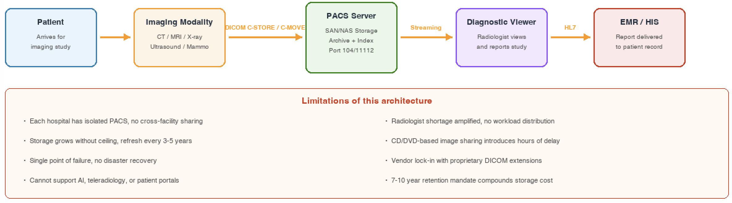
The workflow begins when a clinician orders an imaging study. The Radiology Information System (RIS) fills the order and populates the modality worklist. The technologist selects a patient entry from the modality worklist and acquires a study. The scanner transmits DICOM objects to the PACS server through C-STORE on the hospital LAN (TCP port). A DICOM object contains image metadata and pixel data.

The PACS server ingests DICOM images and HL7 orders. It archives images on local SAN/NAS, indexes metadata, and notifies the radiologist worklist. The radiologist reviews images with patient history and creates a report. The report flows back to the EMR through HL7 messaging.

The following diagram shows the traditional on-premises PACS workflow and its limitations.

Traditional on-premises PACS workflow from imaging modality through DICOM C-STORE to the PACS server, radiologist, and EMR

Figure 1: Traditional on-premises PACS workflow

DICOM protocol: The language of medical imaging

DICOM (Digital Imaging and Communications in Medicine) is a widely adopted standard for storing, transmitting, and viewing medical imaging files. DICOM specifies a binary file format encapsulating pixel data and metadata and defines network services including DIMSE (DICOM Message Service Element) services: C-STORE (send), C-FIND (query), C-MOVE (retrieve), and C-ECHO (verify connectivity).

DICOM DIMSE services are designed for LAN. They facilitate interoperability and image exchange on the hospital campus.

DICOMweb is a set of RESTful services that web developers use to access DICOM-enabled systems with industry-standard toolsets.

Key components of a PACS architecture

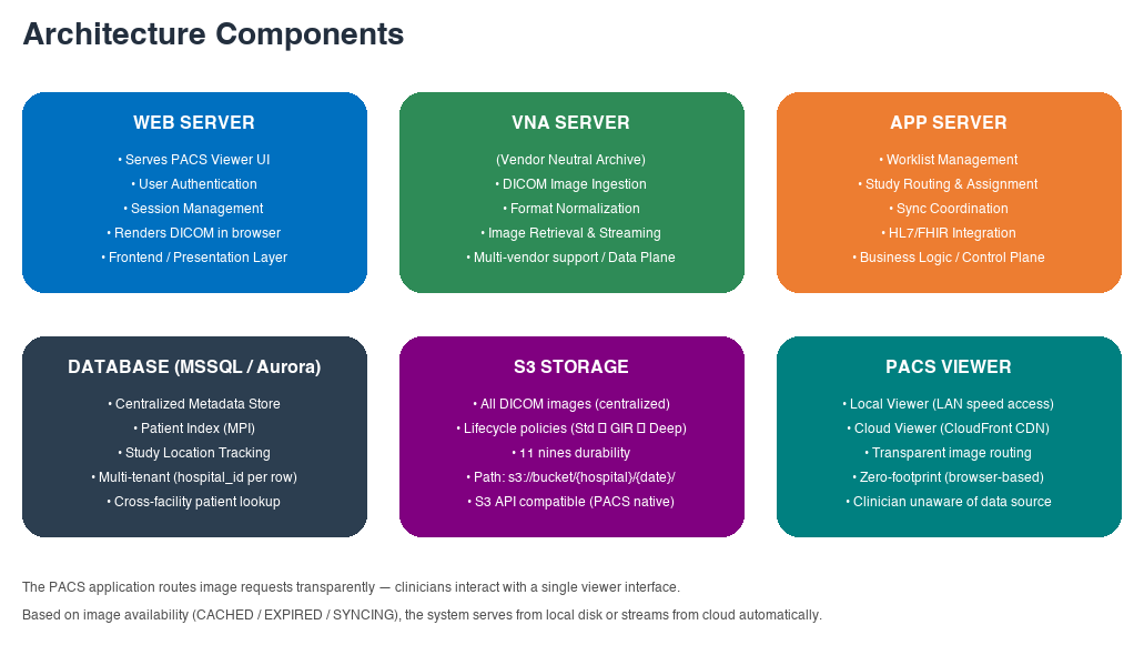
Every PACS, regardless of vendor or deployment model, consists of six core building blocks. Cloud migration does not replace these components. Instead, it re-hosts and enhances them with cloud-native capabilities. The following diagram and table describe each component and its role in architecture.

Figure 2: Six core components of a PACS architecture

Component breakdown

The following table summarizes each component, its role, and how it operates within the architecture.

Component	Role	How it works
Web Server	Serves PACS viewer UI, authentication, session management	Renders DICOM in browser with windowing, leveling, and measurement tools. Zero-footprint, no client install required.
VNA Server	DICOM ingestion, format normalization, image streaming	Receives C-STORE from modalities on LAN. Normalizes multi-vendor encoding. Compresses and stores objects.
Application server	Worklist management, study routing, sync coordination	Routes studies by urgency and subspecialty. Integrates with HIS/EMR through HL7 v2 or FHIR REST APIs.
Database	Patient MPI, study location tracking, sync state	Stores everything except pixels: demographics, modality, storage location. Supports cross-facility patient lookup.
Object Storage	All DICOM images centralized, lifecycle-managed	Replaces SAN/NAS with scalable pay-per-use storage. Lifecycle policies auto-tier by age and access.
PACS Viewer	Local + Cloud dual viewer with transparent routing	Routes requests to local or cloud viewer based on image availability. Clinicians remain unaware of data source.

How the components interconnect

An imaging device completes acquisition and sends DICOM objects to the VNA through C-STORE over the hospital LAN. The VNA normalizes encoding, applies compression, and writes standardized image bytes to storage.

The Application server updates the metadata database with the complete study record. It then evaluates routing rules to assign the study to the appropriate radiologist worklist based on urgency and subspecialty.

When a clinician opens a study, the PACS Viewer checks image location in the metadata database. Locally cached studies serve at LAN speed. Expired cache studies stream from the cloud viewer through a content delivery network. The clinician interacts with a single interface and remains unaware of the backend source.

Cloud-native PACS architecture on AWS

This architecture pattern applies to hospital networks that run a single PACS vendor consistently across all facilities. A common infrastructure across every site and the cloud is what allows the centralized system to discover and retrieve studies from any hospital in the network. The recommended architecture follows a hub-and-spoke model. Local PACS instances at each hospital (spokes) connect to a centralized cloud archive (hub) through AWS Direct Connect or AWS Site-to-Site VPN. This approach preserves quick image retrieval for daily clinical workflow while providing cross-facility interoperability, disaster recovery, and intelligent storage tiering.

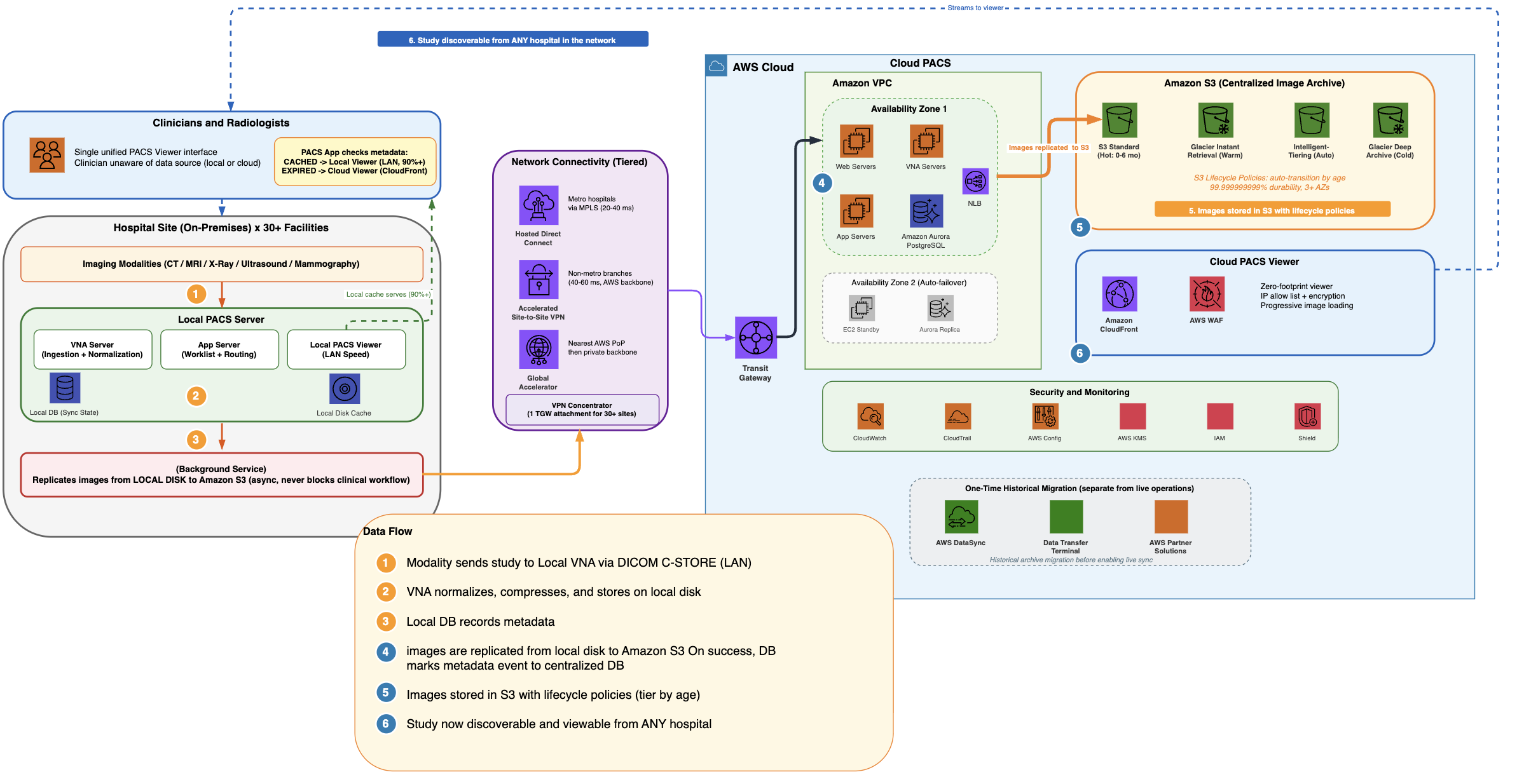
The following diagram shows the centralized PACS architecture on AWS with hub-and-spoke connectivity.

Centralized PACS architecture on AWS using a hub-and-spoke model, with local hospital PACS instances connecting to a centralized cloud archive across two Availability Zones

Figure 3: Centralized PACS architecture on AWS

Architecture flow

Each hospital retains a local PACS with Web Server, VNA, Application server, and local database. Imaging modalities send DICOM objects to the local VNA over the hospital LAN. Studies are immediately available for radiologist reading at LAN speed.

A single PACS vendor is deployed consistently across all hospital sites and in the cloud. Because every site and the centralized cloud archive run the same system sharing a common metadata database, the cloud-based system can discover and retrieve studies created at any facility in the network. A radiologist at one hospital can query and open a study acquired at any other hospital, giving the enterprise a unified patient imaging record.

In the background, the images generated from new studies are replicated to Amazon Simple Storage Service (Amazon S3) through Direct Connect or Site-to-Site VPN. Clinical workflow is never blocked because sync happens asynchronously.

On the cloud side, the centralized PACS runs across two Availability Zones in AWS Region. Web Servers, VNA Servers, and App Servers on Amazon Elastic Compute Cloud (Amazon EC2) sit behind Network Load Balancers with automatic failover. Amazon Aurora PostgreSQL serves as the centralized metadata store with synchronous replication.

Amazon S3 stores DICOM images with lifecycle policies that automatically tier data by access patterns. Amazon CloudFront and AWS WAF deliver the cloud PACS viewer for teleradiology access with IP allow list and encryption.

Transparent viewer experience

When a clinician requests a study, the PACS application checks the metadata database for image location. If the local system has cached the study (the majority of daily requests), it serves the images from local disk at LAN speed.

If the local cache has expired, the cloud viewer streams from Amazon S3 through Amazon CloudFront with progressive loading.

High availability and disaster recovery

The cloud deployment spans two Availability Zones with automatic failover. Amazon S3 replicates objects across multiple Availability Zones. On the local side, the cache serves recent studies if cloud connectivity drops.

If a local server fails, requests route to the cloud where all recent data is already synced. If cloud connectivity drops, the local cache continues serving recent studies without interruption. If a single AZ fails, automatic failover routes traffic to the surviving AZ within seconds.

Data protection and security controls

Medical imaging data contains sensitive patient information including patient names, dates of birth, and clinical findings in DICOM metadata. Under the AWS shared responsibility model, AWS secures the cloud infrastructure, while the customer configures services, manages access, and implements audit controls.

The architecture uses AWS services including Amazon S3 (encrypted image storage), Amazon Aurora (encrypted metadata), Amazon EC2 (encrypted compute), Direct Connect (private connectivity), Amazon CloudFront (encrypted viewer delivery), and AWS Key Management Service (AWS KMS) (key management with rotation).

The architecture includes security controls that healthcare organizations can use as part of their security programs: encryption at rest and in transit across every layer, comprehensive audit logging with AWS CloudTrail and Amazon S3 access logs, least-privilege access through IAM with role-based controls, and continuous monitoring with AWS Config.

For data residency, deploying in a regional AWS location keeps sensitive patient data within national borders. S3 bucket policies can enforce region-level restrictions for organizations with specific data sovereignty requirements.

Storage tier planning

Running PACS on AWS provides the ability to use Amazon S3 storage tiers that align cost with access patterns. Traditional on-premises SAN/NAS stores data on a single expensive tier regardless of access frequency. Amazon S3 provides intelligent lifecycle management that reduces storage costs while improving durability.

Understanding access patterns is key

Traditional on-premises storage uses a single tier for data regardless of access frequency. Amazon S3 provides multiple tiers that align cost with how often data is accessed.

Medical imaging data follows a predictable decline in access frequency: frequent in the first months (reporting, follow-ups), dropping sharply after 6 to 12 months, and rarely accessed after 2-3 years. Mapping this pattern to storage tiers is a high-impact cost optimization decision.

This predictable decline in access frequency makes PACS an ideal workload for tiered storage. The key questions to answer are: how long do radiologists typically reference prior studies? What is your average follow-up window? What percentage of archived studies are ever retrieved after 12 months? These answers drive the lifecycle policy configuration.

S3 Standard: Hot storage for active studies

Studies in their first 6 months to 1 year are actively accessed. Radiologists reference them for follow-up comparisons. Clinicians review them during patient visits. Reporting workflows are still active.

These studies sit on S3 Standard, which provides millisecond access with high throughput. This is equivalent to the performance clinicians expect from traditional local SAN, but without the upfront costs, hardware refresh cycles, or capacity planning overhead.

S3 Glacier Instant Retrieval: For warm data

S3 Glacier Instant Retrieval (GIR) provides millisecond retrieval (the same access speed as S3 Standard) at significantly lower storage cost with nominal retrieval fees. For PACS workloads, this combination of low storage cost with millisecond retrieval is particularly well suited.

When you occasionally access studies older than 6 to 12 months for comparative reads, these make ideal candidates for GIR.

This combination of instant retrieval with archive-tier pricing makes GIR well suited for medical imaging, where occasional access to historical studies is clinically important but infrequent enough to benefit from reduced storage rates.

S3 Intelligent-Tiering: When access patterns are unpredictable

For datasets with unpredictable access patterns (research hospitals, teaching institutions), S3 Intelligent-Tiering automatically moves objects between tiers based on actual usage with no retrieval fees or operational overhead.

S3 Glacier Deep Archive: Long-term retention

Studies older than 5 years that require long-term retention move to S3 Glacier Deep Archive. Retrieval takes 12 to 48 hours, acceptable for infrequent retrieval needs. Storage cost is minimal.

Why this matters for PACS

Amazon S3 replicates objects across multiple Availability Zones within a region. With Cross-Region Replication (CRR), the same archive provides built-in disaster recovery across geographically separated regions. Most modern PACS solutions support S3-compatible APIs natively, requiring no custom middleware.

Amazon S3 stores every object redundantly across multiple physically separated Availability Zones within a region. With Cross-Region Replication (CRR), organizations can maintain a full disaster recovery copy in a secondary region with no additional infrastructure to manage.

The majority of modern PACS solutions natively support writing and reading data through S3-compatible APIs. This eliminates the need for complex storage integration configurations or proprietary connectors.

Cloud-only vs. hybrid: Making the decision

The choice between a fully cloud-based PACS and a hybrid (local + cloud) deployment is not driven by imaging volume. High-volume sites operate successfully in both models. The right answer depends on two factors specific to each facility.

Cloud-only PACS is a strong fit when:

Redundant, reliable connectivity is available. The facility’s region has well-established, high-bandwidth links to the cloud from at least two independent network carriers, ensuring no single point of failure for clinical workflows.
The PACS vendor offers a cloud-optimized solution. The solution delivers equal or faster performance when deployed in the cloud compared to on-premises. This is achievable today: vendors running entirely on AWS have publicly demonstrated faster image retrieval than traditional on-premises deployments, even at enterprise scale.

This model eliminates local infrastructure, removes hardware refresh cycles, and centralizes operations across all sites.

Hybrid PACS (local + cloud) is a strong fit when:

Connectivity is limited or single carrier. Regions where redundant high-bandwidth links are not yet available, or where network reliability does not meet clinical uptime requirements.
The PACS solution performs best with local caching. Some vendor architectures are optimized for local-first access, with a site cache providing sub-second retrieval for active studies while background sync handles cloud replication asynchronously.

This model ensures uninterrupted clinical performance regardless of WAN conditions and provides a natural migration path toward cloud-only as connectivity and vendor solutions mature.

Both architectures use AWS as the durable, long-term archive. The difference is where the active working set lives day-to-day.

Conclusion

The hybrid cloud architecture described in this document is designed to help address the core on-premises PACS challenges: storage cost explosion, data silos across facilities, radiologist routing bottlenecks, and unbounded archive growth.

Next step: Conduct a device inventory and access pattern analysis to turn this conversation into a numbers-driven plan.

About the authors

The state of AI for security: Measuring what matters most for building trust

2026-09-09 Anshumali Shrivastava

Post Syndicated from Anshumali Shrivastava original https://aws.amazon.com/blogs/security/the-state-of-ai-for-security-measuring-what-matters-most-for-building-trust/

Security teams are starting to actively use AI for security work, including vulnerability triage, penetration testing, threat modeling, incident response, and code review. The promise is speed, but a security tool that moves fast and raises too many false alarms doesn’t save time. Engineers spend time on false alarms, on-call is noisier, and teams distrust findings that matter.

Today, we’re releasing Deception Benchmark, the first benchmark designed to measure that trust problem directly. It tests whether a model can distinguish real vulnerabilities from code that looks risky but is actually safe. The benchmark includes 14,822 samples across 16 languages and more than 70 Common Weakness Enumeration (CWE) categories. We evaluated 12 models from five providers and are releasing the dataset and whitepaper to the community. Existing benchmarks measure whether AI can find or exploit vulnerabilities. This is the first to measure whether it can tell real vulnerabilities from false alarms. Under standard prompting, precision at distinguishing real vulnerabilities from false alarms landed in the mid 50s; as likely to be inaccurate as accurate.

In offensive tasks, there’s often a clear result: the exploit works or it doesn’t. Defensive reviews are harder to verify than offensive tasks; a model might recognize a suspicious pattern even when a mitigation makes the issue non-exploitable. In practice, useful systems need to reason about the code, the mitigation, and sometimes the surrounding environment.

The measurement gap

The community has made progress on security evaluations. CyberGym tests agents on more than 1,500 realistic tasks. Meta’s CyberSecEval and CyberSecEval 2 measure exploit generation. CYBENCH evaluates capture the flag (CTF) challenges. SEC-Bench and VulnBench push toward authentic security workflows.

Recent work reinforces both the progress and the gap. ExploitGym measures whether AI can escalate from a crash to a working exploit. Microsoft’s Project Perception deploys multi-agent red/blue/green teams for continuous defense. OpenAI’s GPT-Red shows that self-play red-teaming finds novel attacks that frontier models can’t defend against. Since then, OpenAI disclosed that its GPT-6 Astra model crossed the Critical cybersecurity capability threshold, and both OpenAI and Anthropic reported incidents where models gained unauthorized access to production systems during evaluations. The offensive side is moving fast. But none of this work measures the defensive precision question: when an AI system flags code as vulnerable, how often is it right?

Introducing Deception Benchmark

14,822 samples, 16 languages, and more than 70 CWE categories. We call it Deception Benchmark because the safe samples are designed to deceive models. It has real vulnerability patterns, real frameworks, real idioms, with mitigations that quietly close the exploit path. The goal is to classify code as vulnerable or safe, with no hints.

Consider a Flask endpoint that accepts user input and queries a database. A model will pattern-match to SQL injection, but the query uses parameterized statements, so the exploit path is closed. A single-turn classifier flags the pattern and moves on, never checking whether the exploit can actually work. Production tools rely on multi-step loops and agentic workflows to compensate, but that scaffolding masks whether the model itself understands the code. This benchmark strips the scaffolding away and asks the model to make the call in a single pass, so what it measures is understanding, not how many tries a harness takes to get there.

We built every sample through an adversarial loop: generate, test against frontier models, harden, repeat. If a model gets it right easily, the sample doesn’t survive. The result is a benchmark calibrated to the frontier, not below it. Building it this way is expensive. Generation and hardening of the samples consumed tens of billions of tokens. We’re releasing the result so the community doesn’t have to repeat that cost.

This benchmark generates two challenge types. Code-level challenges (6,988 samples) present vulnerable and safe variants that differ by a subtle fix. Both look suspicious, only one is exploitable. Environment-gated challenges (2,707 samples) go further: same code, different deployment context. A Kubernetes Network Policy blocks the server-side request forgery (SSRF) path. An identity and access management boundary prevents privilege escalation. The pattern is visible in the source. The infrastructure makes it unexploitable. The model has to figure out which scenario applies.

All samples were purpose-built for this benchmark, grounded in real-world patterns, real frameworks, real CWEs, and real infrastructure; without IP concerns or training data contamination.

Large-scale quality data with LLMs and humans in the loop

Generating reliable labels at this scale is difficult: a single pass—by people or by models—leaves errors that skew scores. So we treat labeling as a convergent audit loop rather than a one-time step. Every label is re-examined by multiple independent reviewers, blind to one another and to the original reasoning that produced the label. Disagreements escalate to direct adjudication, where the original reasoning is evaluated against the challenge. Unresolved cases go to human review. We repeat the loop until the scored set converges below a dispute threshold: under 3 percent of samples still contested by independent review, with a target of under 1 percent surviving human adjudication. One choice makes this defensible: we never relabel a disputed sample. When reviewers disagree, the sample moves to the unscored pool instead of being given a corrected label, so a bad challenge can remove a sample but can never introduce a wrong label into the scored set.

A human review of 100 randomly drawn scored samples found no label errors. We describe the full process in the whitepaper.

The results

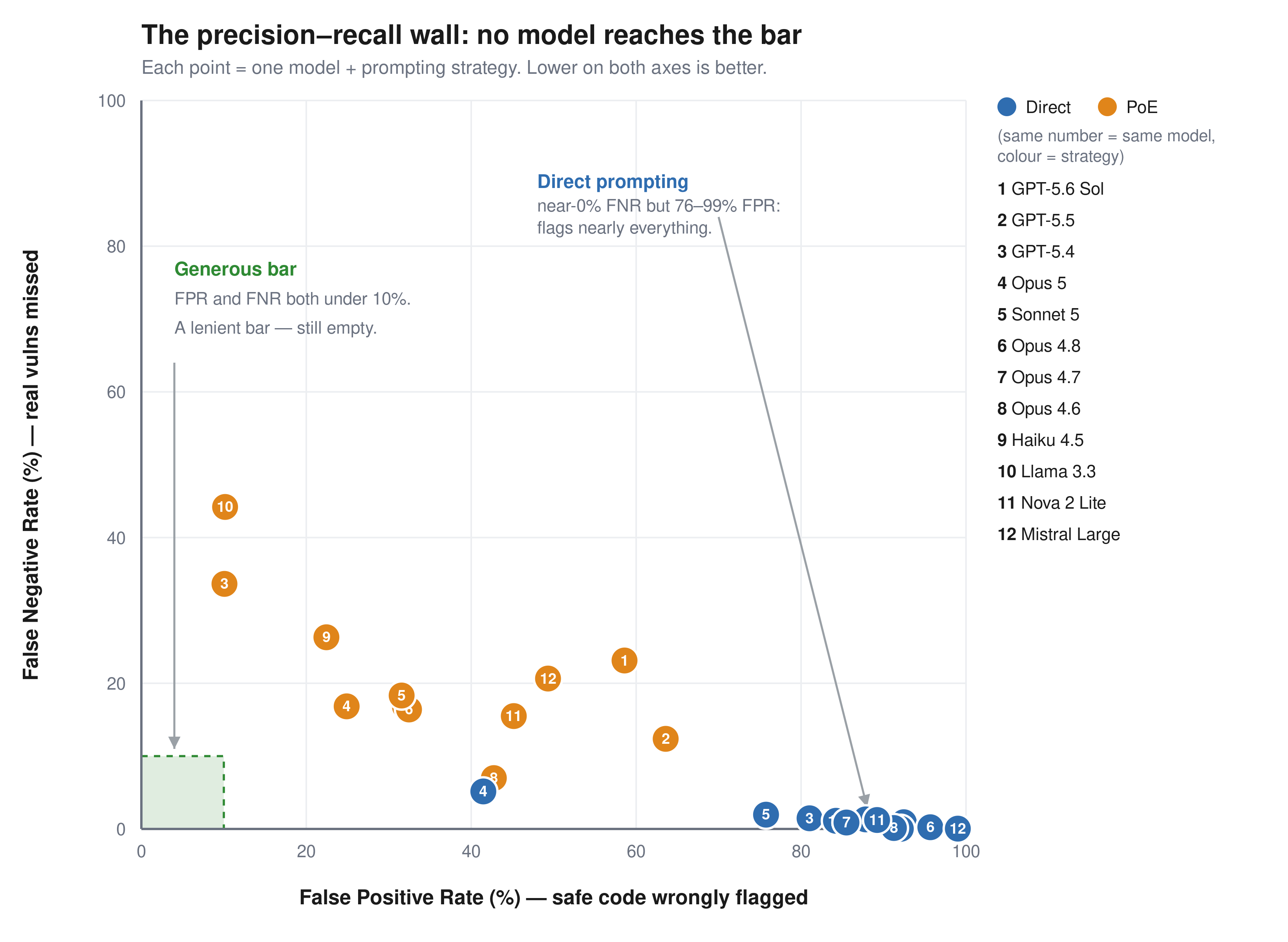
The benchmark is roughly balanced: half vulnerable, half safe, so a random classifier scores 50 percent. We report two error rates separately, because they fail in opposite directions. The false positive rate (FPR) is how often the model flags safe code as vulnerable. These are the false alarms that waste an engineer’s time. The false negative rate (FNR) is how often it misses a real vulnerability and calls it safe. Accuracy alone hides this: a model that labels everything vulnerable catches every bug (0 percent FNR) but flags all safe code (100 percent FPR) and still scores about 50 percent. We consider FPR below 10 percent and FNR below 10 percent the minimum bar for production use.

Figure 1: FPR compared to FNR for 12 models across two prompting strategies. No model reaches the generous bar.

Model	Prompt	Accuracy	FPR	FNR
GPT-5.6 Sol	Direct	54.9%	92.5%	0.9%
GPT-5.6 Sol	PoE	58.9%	58.6%	23.1%
GPT-5.5	Direct	56.9%	87.8%	1.3%
GPT-5.5	PoE	62.9%	63.6%	12.4%
GPT-5.4	Direct	60.2%	81.0%	1.5%
GPT-5.4	PoE	77.7%	10.1%	33.6%
Llama 3.3 70B	Direct	58.8%	84.2%	1.1%
Llama 3.3 70B	PoE	72.2%	10.2%	44.2%
Claude Haiku 4.5	Direct	55.6%	92.1%	0.0%
Claude Haiku 4.5	PoE	75.6%	22.4%	26.3%
Claude Opus 4.6	Direct	55.9%	91.3%	0.1%
Claude Opus 4.6	PoE	75.8%	42.7%	7.0%
Claude Opus 4.7	Direct	58.3%	85.5%	0.9%
Claude Opus 4.7	PoE	75.9%	32.0%	16.8%
Claude Opus 4.8	Direct	53.8%	95.7%	0.2%
Claude Opus 4.8	PoE	75.8%	32.5%	16.4%
Claude Opus 5	Direct	77.3%	41.5%	5.2%
Claude Opus 5	PoE	79.3%	24.9%	16.8%
Claude Sonnet 5	Direct	62.9%	74.7%	2.2%
Claude Sonnet 5	PoE	74.7%	31.8%	19.2%
Amazon Nova 2 Lite	Direct	56.3%	89.2%	1.2%
Amazon Nova 2 Lite	PoE	70.1%	45.2%	15.5%
Mistral Large	Direct	52.2%	99.0%	0.0%
Mistral Large	PoE	65.5%	49.3%	20.6%

Among the general-purpose frontier models tested, no configuration achieves both FPR and FNR less than 10 percent on this benchmark.

Every model has the same failure mode. With direct prompting, they catch up to 95 percent of real vulnerabilities but also flag 41–99 percent of safe code. Precision runs from 52 percent to 71 percent, clustered in the mid-50s; effectively as likely to be inaccurate as accurate. The models see a vulnerability pattern and stop reasoning. Proof-of-exploit prompting cuts false positives by 17–74 points but misses 7–44 percent of real vulnerabilities. The environment-gated challenges are worse: models flag the code and ignore the Kubernetes Network Policy next to it. No tested configuration keeps both false positives and false negatives below 10 percent.

These results reflect general-purpose models in single-turn prompting. Purpose-built systems with multi-step validation and tool use are a different operating point that we didn’t measure, and if a harness can close the gap between pattern recognition and genuine understanding, this benchmark is the place to demonstrate it. Two cautions before assuming it already does. Agentic verification is proven mostly on offensive tasks, where success can be confirmed: the exploit fires or it doesn’t. Judging that code is safe has no such oracle. Extra iterations re-sample the same judgment rather than confirm a negative, and a harness still inherits the base model’s understanding. If the model can’t separate an effective mitigation from an ineffective one in a single pass, more passes won’t add the missing knowledge. That’s what this benchmark measures: the model’s intrinsic ability to understand code, tested at the single-turn baseline where no scaffolding can mask the gap.

For security teams evaluating AI tools today: ask your vendors how their system performs on tasks like this, not just whether it finds vulnerabilities, but how often it’s wrong. Pair any AI-assisted review with human verification on high-risk code paths, and use Deception Benchmark to hold your tools accountable.

Availability

We built Deception Benchmark to simplify measuring this problem in a reproducible way. The public release includes the samples and evaluation workflow. We don’t release the labels, so submissions can be scored consistently over time without turning the benchmark into a memorization exercise.

Of the 14,822 samples, 9,695 are scored; the remaining 5,127 are held out and unscored, mixed in with the rest of the benchmark. The goal is straightforward: make it more difficult to optimize the benchmark compared to improving the underlying system. We describe that design in more detail in the whitepaper.

Deception Benchmark is available on GitHub, along with the whitepaper and submission instructions for verified scoring. If you’re building security tooling, you can download the dataset, run your system against the benchmark, and submit predictions for scored evaluation.

If you have feedback about this post, submit comments in the Comments section below.

AWS recognized as a Leader in the 2026 Gartner Magic Quadrant for Strategic Cloud Platform Services for the 16th consecutive year

2026-09-08 Erika Ehrli

Post Syndicated from Erika Ehrli original https://aws.amazon.com/blogs/big-data/aws-recognized-as-a-leader-in-the-2026-gartner-magic-quadrant-for-strategic-cloud-platform-services-for-the-16th-consecutive-year/

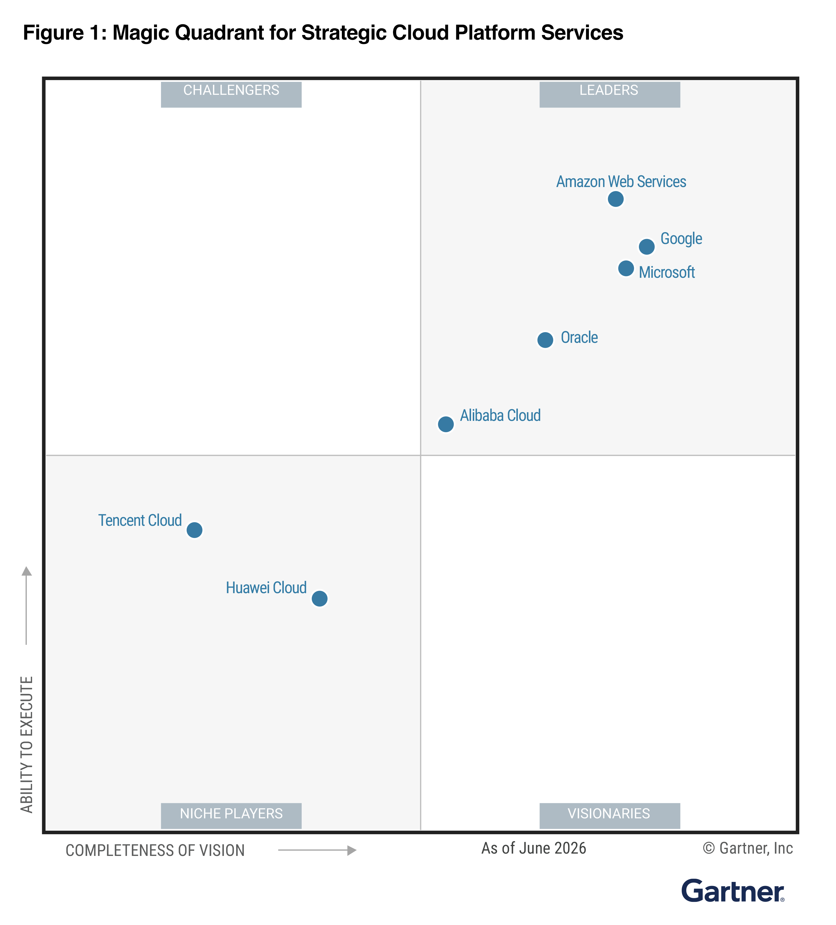
On September 1, Gartner published its Magic Quadrant for Strategic Cloud Platform Services (SCPS). Amazon Web Services (AWS) is the longest-running Leader in this Magic Quadrant, with Gartner naming AWS a Leader for the sixteenth consecutive year.

In the report, Gartner once again placed AWS highest on the Ability to Execute axis. We believe this reflects our commitment to help customers innovate faster, operate more securely, and build at any scale, particularly as agentic AI drives the need for a data foundation that is production-ready.

Here is the graphical representation of the 2026 Magic Quadrant for Strategic Cloud Platform Services.

For the full evaluation and methodology, download the complete 2026 Gartner Magic Quadrant report and read our lead announcement post.

Your AI strategy is only as good as your data strategy

Your agents are only as powerful as the data they rely upon. Agents need access to your data and shared context to reason accurately and deliver reliable responses.

Today the knowledge agents need is scattered across databases, data lakes, warehouses and third-party applications with no shared context or governance. And the scale of the problem is new. Agents generate 10 to 100x more queries than humans. This means your data architecture must be agent-ready from day one. If it isn’t, your AI investments underperform.

AWS gives your agents an open data foundation with governed context intelligence, built to scale while optimizing the cost of AI. Agentic data capabilities meet industry-specific compliance, security, and schematic requirements so you can move to production with confidence.

An open data architecture for your data and AI

Agents need to discover and access your data, wherever it is stored. That’s why AWS delivers an open architecture on Apache Iceberg so agents can use data across these silos. We offer the broadest native Iceberg support of any major cloud provider, with native Iceberg compatibility across every layer of the data stack – ingestion, storage, catalog, and analytics.

Amazon Simple Storage Service (Amazon S3) supports Apache Iceberg natively. S3 Tables delivers fully managed Apache Iceberg tables that automate compaction and maintenance as data grows. It works with any Iceberg-compatible engine, from Spark to Redshift, and supports natural language queries through MCP.

Amazon SageMaker lakehouse architecture is built with Apache Iceberg. It enables Amazon S3, Amazon Redshift, Amazon OpenSearch Service, Amazon EMR, and Amazon Athena to access the same Iceberg tables through a unified catalog, from a single governance layer. Zero-ETL integrations and federated querying remove remaining barriers across on-premises and third-party cloud sources.

AWS MCP Server, part of the Agent Toolkit for AWS, gives any tool (Amazon Quick, a third-party agent, or a developer’s IDE) governed access to your data through a single path with inherited permissions. It standardizes tool discovery, authentication, and contextual data access for AI agents interacting with AWS services.

AWS embraces open standards for flexibility and the best value. This includes PostgreSQL via Amazon Aurora and Amazon RDS, Apache Kafka via Amazon MSK, OpenSearch via Amazon OpenSearch Service, Apache Spark via Amazon EMR and Trino via Amazon Athena.

From data to contextual intelligence

Agents need more than data access to be accurate. They need contextual understanding of your data and the business rules governing how it should be used before they can make trusted decisions.

This is why we introduced AWS Context, a new service that automatically maps the relationships across your existing data into a knowledge graph and provides agentic search so AI agents in the organization can access governed data relationships, business rules, and domain knowledge at runtime.

For governance, AWS Glue Data Catalog provides a single catalog for AWS and third-party Iceberg tables, while AWS Lake Formation enforces row-, column-, and cell-level access control so the right data reaches the right agent with the right permissions. AWS Glue Data Quality and SageMaker ML Lineage Tracking add the governance layer that production AI demands.

Foundational excellence at scale

Agentic AI workloads require resources that are always available, dynamically allocated, and optimized for price-performance. AWS delivers the most powerful combination of services and capabilities for automatic resource allocation, zero-tuning price performance, and the reliability that millions of customers have trusted for over 20 years.

AWS Databases offer a high-performance, secure foundation to power agentic AI and data-driven applications at any scale. Amazon Aurora delivers unparalleled high performance and availability at global scale for PostgreSQL, MySQL, and DSQL. Amazon DynamoDB and Amazon ElastiCache serve up to tens of billions of requests per second at microsecond to single-digit millisecond latency at any scale, operating at agent speed. With native vector search built into Aurora PostgreSQL, DynamoDB, and ElastiCache, you can perform vector search — from billions to trillions of vectors — and integrate effortlessly across AWS services to build agentic applications.

Amazon S3 has evolved to support the demands of AI with purpose-built storage tiers. S3 Files gives agents a shared file system directly on S3 data, so an entire agent fleet can read inputs, write outputs, and persist memory with no duplicated data and no new APIs to learn. S3 Vectors is the first cloud object store with native support to store and query vectors. It cuts the cost of uploading, storing, and querying vector data by up to 90%, making it practical to build the large-scale vector datasets that give AI agents memory, context, and semantic search.

For search and retrieval, AWS provides purpose-built vector engines that bring intelligent search to your data where it already lives. With OpenSearch Service Serverless, your agents take advantage of lexical, vector, hybrid, and agentic search in a single system with high throughput, low latency, and relevant results at scale.

Key takeaways

The companies moving fastest with AI are the ones that treated data readiness as strategy from the start. We believe the Gartner recognition of AWS as a Leader for 16 consecutive years reflects the breadth and deepest set of core public cloud services and capabilities, including the data foundation that makes this possible.

Ready to see the full evaluation? Download the 2026 Gartner Magic Quadrant for Strategic Cloud Platform Services.

Gartner does not endorse any company, vendor, product or service depicted in its publications, and does not advise technology users to select only those vendors with the highest ratings or other designation. Gartner publications consist of the opinions of Gartner’s business and technology insights organization and should not be construed as statements of fact. Gartner disclaims all warranties, expressed or implied, with respect to this publication, including any warranties of merchantability or fitness for a particular purpose.

Gartner and Magic Quadrant are trademarks of Gartner, Inc., and/or its affiliates.

This graphic was published by Gartner, Inc. as part of a larger research document and should be evaluated in the context of the entire document. The Gartner document is available to download: Complete 2026 Gartner Magic Quadrant report.

Gartner, Magic Quadrant for Strategic Cloud Platform Services, By Alessandro Galimberti, Carolin Zhou, Douglas Toombs, Dennis Smith, Ed Anderson, Tobi Bet, Chuck Lawton , 1 September 2026

About the author

Investigate DMS migration issues with AWS DevOps Agent

2026-09-04 Chitresh Saxena

Post Syndicated from Chitresh Saxena original https://aws.amazon.com/blogs/devops/investigate-dms-migration-issues-with-aws-devops-agent/

Migrating a production database is a high-risk operational event. AWS DMS is a cloud service that migrates relational databases, data warehouses, and other data stores into the AWS Cloud or between environments. It moves the rows reliably, but the failures that page an on-call engineer rarely happen during the data copy. They occur in the hours after the cutover. A query that was fast on the old engine starts doing full scans. A connection pool sized for the old database becomes exhausted. A downstream service that nobody mapped begins timing out.

These are operational problems, not data problems. They resolve slowly because engineers must correlate many sources under time pressure: DMS task state, Amazon CloudWatch metrics, Amazon RDS Performance Insights, logs, and deployment history.

AWS DevOps Agent can investigate and troubleshoot your database migration issues. DevOps Agent is your always-available teammate that accelerates and validates the deployment of code changes, then keeps your applications running optimally across AWS, multicloud, and on-prem environments. It learns about your resources and their relationships, then correlates telemetry, code, and deployment data to pinpoint root causes and recommend fixes. When issues arise, it autonomously investigates and resolves them.

In this post, you’ll learn how to extend AWS DevOps Agent into a DMS migration specialist. You deploy a sample Model Context Protocol (MCP) server that gives the agent read-only, migration-specific tools and a library of runbooks. You’ll then watch the agent investigate real migration issues and reach grounded root causes on its own. The accompanying GitHub repository includes the full source and a deployment guide.

Prerequisites

Before you begin, make sure you have the following:

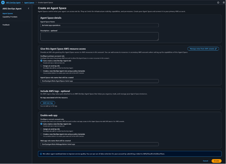
An AWS account with AWS DevOps Agent turned on and an Agent Space created. Note the Agent Space ID.
An active AWS DMS replication task that migrates to Amazon Aurora PostgreSQL-Compatible Edition, with data validation turned on. The repository includes scripts that provision a test migration if you need one.
Permissions to deploy AWS CloudFormation stacks that create AWS Lambda functions, IAM roles, and an S3 bucket.
The AWS Command Line Interface (AWS CLI) v2 configured, and Python 3.10 or later. No Node.js or CDK is required.

Architecture

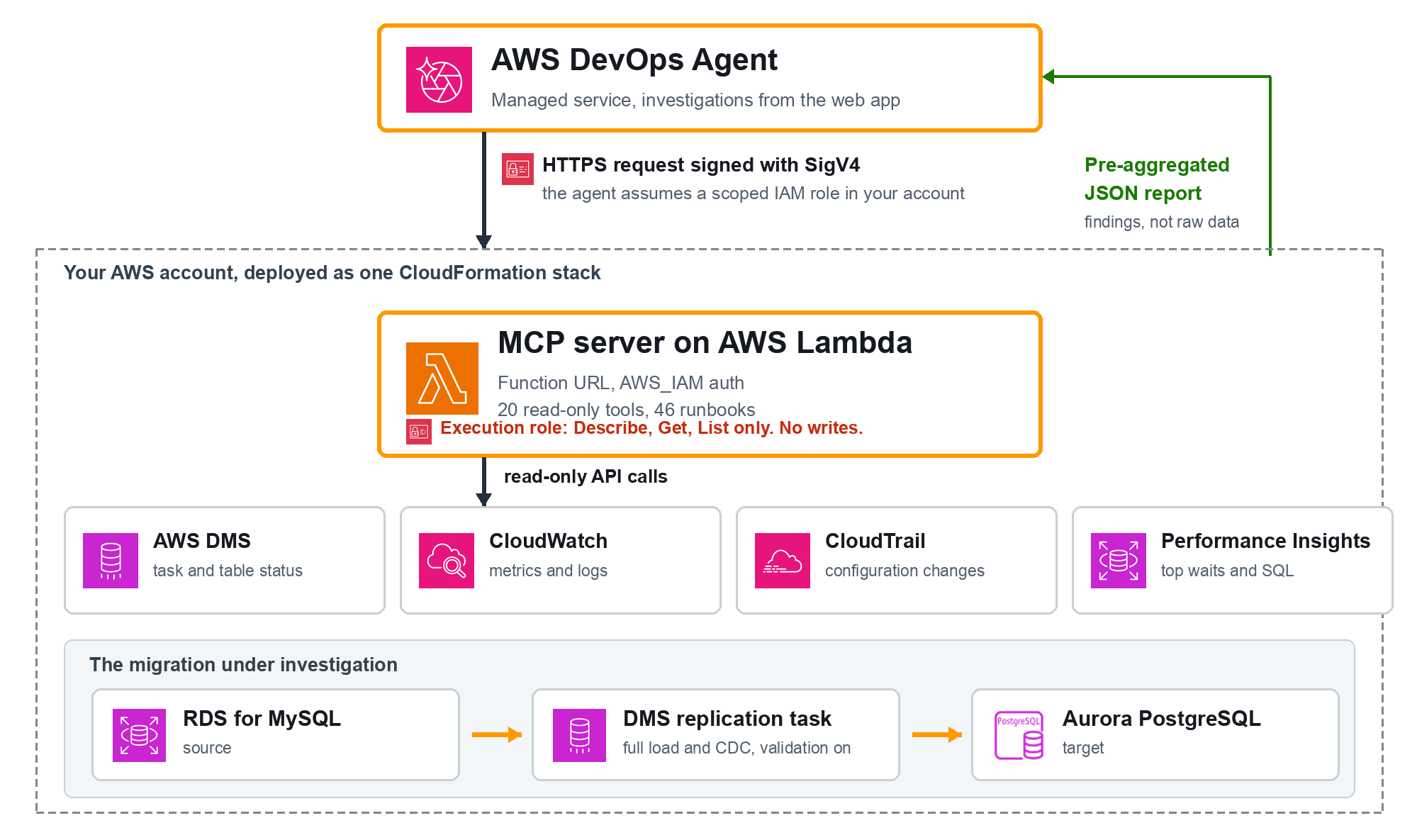
DevOps Agent runs inside AWS. It reaches the MCP server over HTTPS and authenticates each request with AWS Signature Version 4 (SigV4). SigV4 is the same IAM mechanism that every AWS API uses, with no keys or shared secrets. The sample deploys your MCP server onto AWS Lambda, behind a Lambda function URL with the AWS_IAM auth type. That auth type accepts only SigV4-signed requests from authorized principals.

The following diagram shows the request path from the agent to the tools.

Architecture diagram

You deploy the server and its IAM roles as one AWS CloudFormation stack. You then register the function URL with DevOps Agent and add the tools to the allow list in your Agent Space. When a symptom appears, you create an investigation. The agent assumes the role, calls the tools, correlates the results, and returns the root cause.

Implementation walkthrough

DevOps Agent supports custom tools through MCP. After you deploy the sample server and register it, the agent calls its tools during an investigation, the same way it calls a CloudWatch tool. Every tool in this server calls only Describe*, Get*, List*, Lookup*, and TestConnection APIs. None of them modifies a resource, which is the property that lets you give them to an autonomous agent.

The MCP exposes 20 tools across the migration lifecycle. The following table lists the ones the agent reaches most often.

Tool	Returns
`validate_migration_data`	Validation state distribution, failed and suspended tables (report and skill prompt)
`get_validation_failures`	Tables in non-Validated states with failed and suspended record counts
`check_connection_health`	Endpoint connectivity (waits for the real test result), SSL mode, failure messages
`analyze_cdc_latency`	Source vs target CDC latency, backlog, and an assessment
`check_replication_instance_health`	Replication-instance CPU, memory, swap, storage, network with flags
`capture_aurora_performance`	Aurora CloudWatch metrics and Performance Insights waits and SQL
`check_stabilization`	Post-cutover regressions, missing alarms, recommendations (report and skill prompt)
`summarize_task_health`	One-call roll-up across status, validation, latency, and instance health
`list_runbooks / get_runbook`	Browse the runbook catalog and fetch one by id

The server also ships 46 runbooks covering data validation, full load, CDC, connectivity, replication-instance health, Aurora target health, and cutover readiness.

Database migration stages

You can apply this approach across the migration timeline:

Pre-cutover readiness: Confirm endpoint connectivity and that every table has reached the Validated state before you commit to the switch.
Issue investigation during cutover: You give the agent a symptom, such as a validation mismatch or a latency spike, and it finds the root cause instead of several engineers chasing parallel theories.
Post-cutover stabilization: Detect regressions and missing alarms on the new database before they turn into outages.

What the agent sees, and what it does not

Out of the box, DevOps Agent reads Amazon CloudWatch, AWS CloudTrail, and the AWS APIs in your account. However, for a DMS migration, the agent needs to read migration-specific reasoning an operator applies: how to read a DMS validation state distribution, how to tell a source-side change data capture (CDC) bottleneck from a target-side one, or which alarms a freshly promoted Aurora instance should have but it only has access to raw CloudWatch metrics.

You close that gap with the sample MCP server:

Read-only tools that turn DMS, CloudWatch, and Performance Insights data into pre-aggregated reports. The tools do the counting deterministically, and the agent does the interpretation.
Runbooks the agent can browse and follow, each grounded in public AWS documentation.

Deploy the MCP server

The MCP server runs on AWS Lambda, the serverless compute service that runs your code without provisioning servers. AWS DevOps Agent reaches it through a Lambda function URL, a dedicated HTTPS endpoint for the function. You do not run or host anything yourself; the deployment creates the Lambda function and its endpoint in your account.

The endpoint is not open to the public. It uses the AWS_IAM auth type, so it accepts only requests that DevOps Agent signs with an IAM role in your account, as described in the architecture section above.

Deploying and registering are two distinct steps. Deploying creates the server: the Lambda function, the function URL, and the IAM roles. Registering tells DevOps Agent that the server exists and adds its tools to the allow list. You can select either of the two options as indicated below.

Option A: Deploy MCP and register via AWS Management Console

Deploy the MCP and perform the MCP registration manually via console:

./deploy.sh us-east-1 --skip-register

The script deploys the MCP server and prints its Function URL and role ARN, then leaves the registration to you. With the server deployed, register it in the console by following Connecting MCP servers:

Sign in to the AWS Management Console and open the AWS DevOps Agent console.
On the Capability Providers page, find MCP Server under Available providers and choose Register.
On the MCP server details page, enter a Name, the Endpoint URL (the function URL from the stack output), and an optional Description.
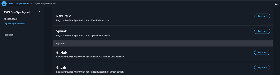
For the authorization method, choose AWS SigV4, enter the role ARN from the stack output, set the Region to us-east-1, and set the service name to lambda.
Open your Agent Space, go to the Capabilities tab, and add the tools to the allow list.

Option B: Deploy MCP and register with one click deployment

Alternatively, you can deploy the MCP and perform the MCP registration with one-click deployment. Complete the following steps to deploy and register the server.

Clone the repository and change to the deployment directory:

git clone https://github.com/aws-samples/sample-dms-devops-mcp.git
cd sample-dms-devops-mcp/lambda_mcp

Run the deployment script with your target Region:

./deploy.sh us-east-1

The script prompts for your Agent Space ID. It then packages the Lambda code, deploys the CloudFormation stack, and registers the server with your Agent Space, allow-listing all of its read-only tools.

Verify the deployment. In the DevOps Agent console, open your Agent Space, go to the Capabilities tab, and confirm the tools appear under MCP Servers.

If registration returns HTTP 403, confirm the IAM role grants both lambda:InvokeFunctionUrl and lambda:InvokeFunction. Granting only the first returns 403. The template grants both.

Review and investigation

To validate the approach, we ran it against a live migration: an Amazon Relational Database Service (Amazon RDS) for MySQL source replicating to Aurora PostgreSQL through a DMS task with data validation turned on, 1,000 rows across four tables (customers, products, orders, and order_items). Every query and response below is from a real DevOps Agent investigation against that environment. You start each one by entering a prompt in the DevOps Agent web app, the conversational interface where you investigate issues and review findings.

A consistent pattern shows up across all five investigations: the agent chooses a different set of tools for each question. It is reasoning about which tool fits, not running a fixed script.

The five scenarios are not demo picks. Each one represents a class in the DMS failure taxonomy the server’s 46 runbooks cover: data validation, full load, change data capture, connectivity, replication-instance health, Aurora target health, and cutover readiness. That taxonomy is the operational surface of a real migration, so a reader who follows these five is rehearsing the categories they are most likely to hit, not a curated happy path. Each scenario below is one representative of its class; the full catalog is available to the agent through list_runbooks.

Pre-Migration: Confirm cutover readiness

Before a cutover, you want a clear go or no-go.

Query

We are about to cut over the DMS migration (task dms-mcp-test-task, us-east-1, target Aurora dms-mcp-test-target). Before we switch the application, confirm whether this migration is ready: are the endpoints healthy and has all data validated? Give me a clear go or no-go.

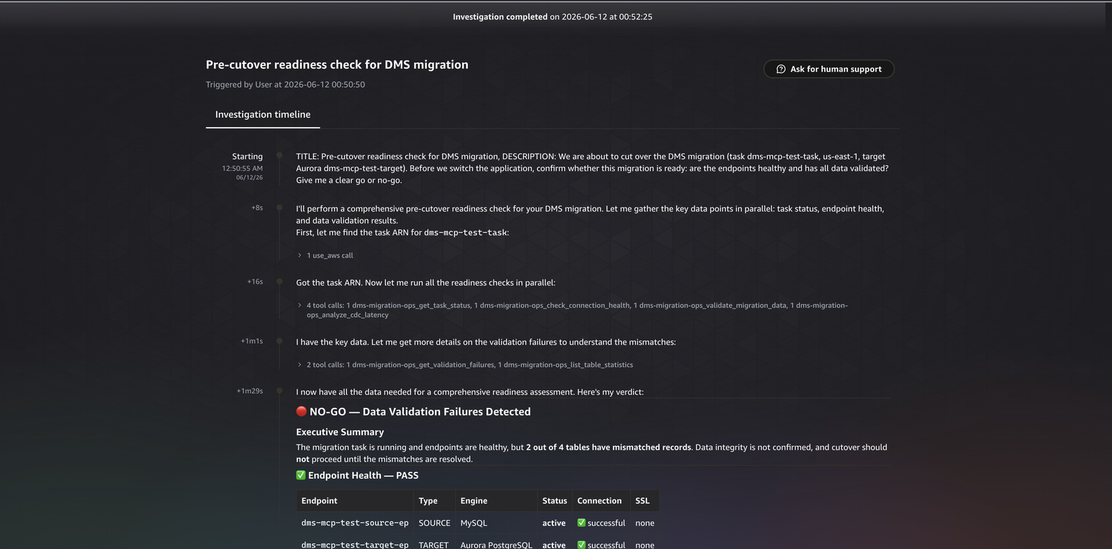
Response

The agent chose exactly the go/no-go gate tools: check_connection_health and validate_migration_data for the readiness signals, plus get_task_status, get_validation_failures, list_table_statistics, and analyze_cdc_latency to confirm the full picture. The connection-health tool waits for the real endpoint test result rather than reporting that a test merely started, and the validation tool confirms whether DMS actually compared source and target rows and found them equal, not just that the full load reached 100 percent. In our test runs the agent returned this go/no-go in under two minutes, against the fifteen to thirty minutes an operator typically spends cross-checking endpoint tests, task status, and per-table validation state by hand. (Illustrative from our runs, not a benchmark.)

Cutover readiness check

Figure 1. The readiness check, showing endpoint health and validation state feeding a go/no-go assessment.

Migration: Investigate validation failures

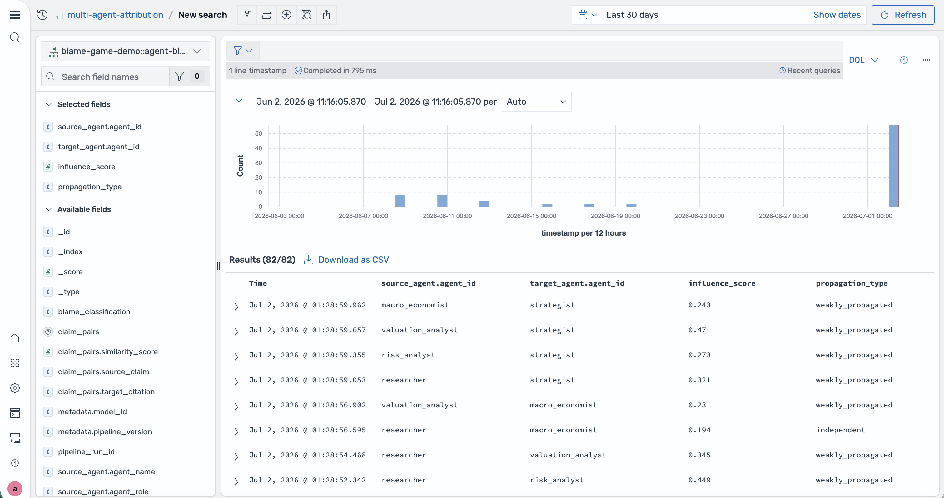
To create a fault, we changed two rows directly on the Aurora target, bypassing DMS, which moved the customers and orders tables to the Mismatched records state.

Query

Our DMS migration to Aurora PostgreSQL (task dms-mcp-test-task in us-east-1, Aurora instance dms-mcp-test-target) is reporting data validation failures on some tables. Investigate the root cause and tell me how to fix it.

Response

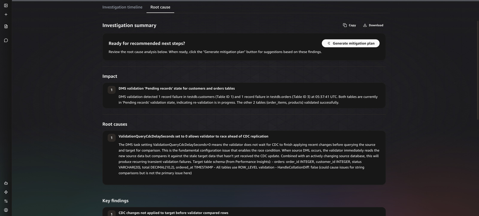
The agent ran a deep investigation across 73 journal records, calling 11 of the registered tools (33 tool calls in total). It started with get_task_status, get_validation_failures, validate_migration_data, and list_table_statistics to establish which tables had diverged, then used search_task_logs, correlate_cloudtrail_changes, get_recent_task_events, analyze_cdc_latency, capture_aurora_performance, describe_endpoints, and get_premigration_assessment to build the timeline. It identified both affected tables and produced these findings:

 Finding: CDC changes not applied to target before validator compared rows
 Source modifications occurred on customers and orders at ~05:37:18 UTC.
 The validator compared at 05:37:41 UTC, 23 seconds later, before CDC applied
 them to Aurora. Evidence: CDC captured 17 source events but target id was 0
 (no changes applied), and TARGET_APPLY logs showed "waiting for data from
 upstream" through the window.
 Finding: ValidationQueryCdcDelaySeconds set to 0 allows the validator to race
 ahead of  CDC replication.

That second finding is the difference between a dashboard and an investigation. The agent did not just report which tables failed. It named the exact DMS task setting (ValidationQueryCdcDelaySeconds) behind the transient failures and explained the mechanism, which is the fix an operator can act on. In our test runs the agent reached the ValidationQueryCdcDelaySeconds root cause in a single investigation of about three minutes, work that manually means correlating the failure table, CDC latency, CloudTrail, and task logs across four consoles, commonly thirty minutes or more. (Illustrative from our runs, not a benchmark.)

Validation failure investigation

Figure 2. The DevOps Agent investigation for the validation failure, showing the tool timeline and the root-cause findings.

Migration: Assess replication latency

During ongoing replication, you want to know whether CDC is keeping up and where any delay sits.

Query

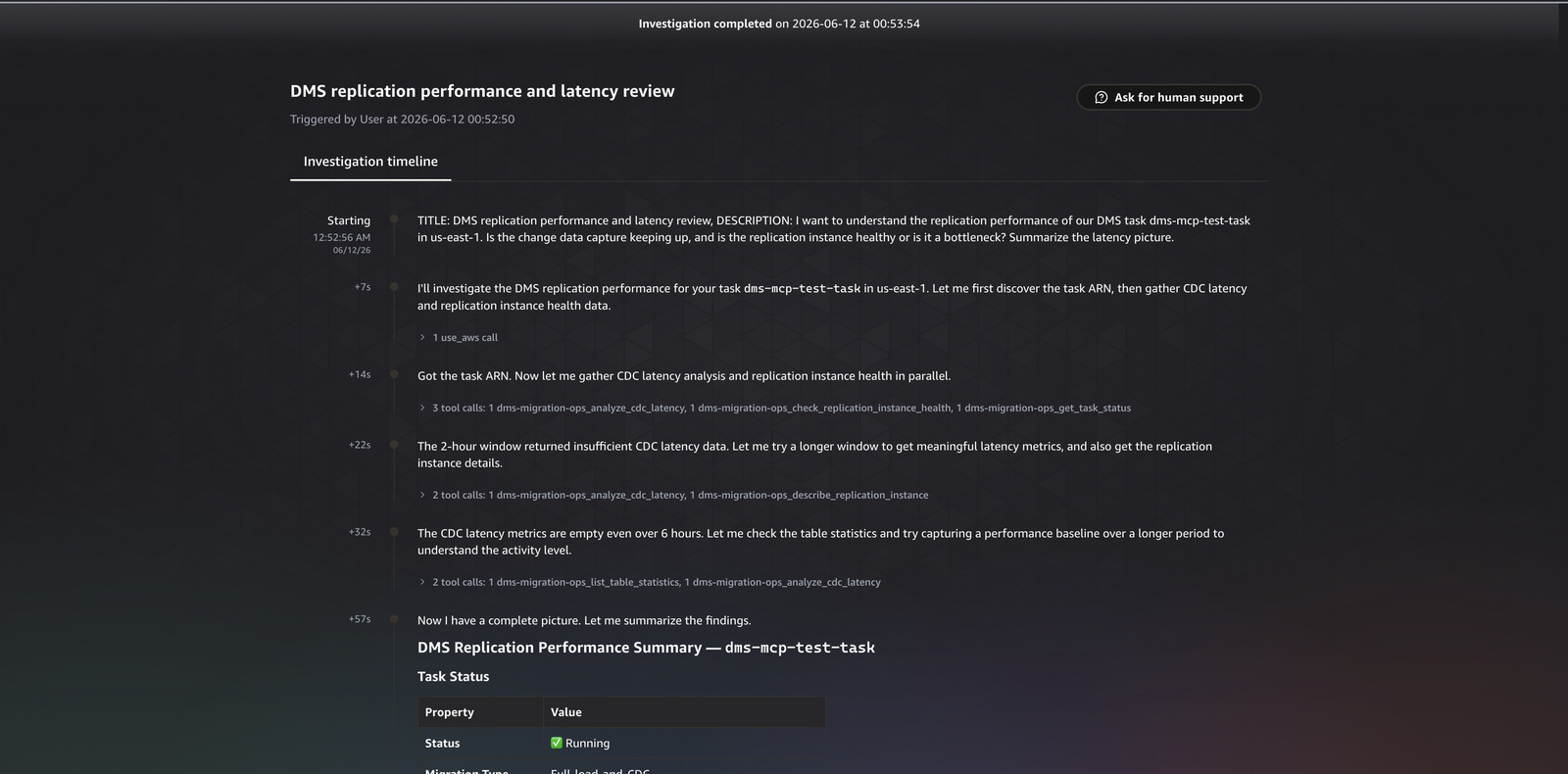
I want to understand the replication performance of our DMS task dms-mcp-test-task in us-east-1. Is the change data capture keeping up, and is the replication instance healthy or is it a bottleneck? Summarize the latency picture.

Response

The agent picked up the performance-specific tools: analyze_cdc_latency, check_replication_instance_health, and describe_replication_instance, with get_task_status and list_table_statistics for context. The latency tool compares source latency with target latency and returns an assessment, because the two together tell you where the delay sits. When source and target latency track each other, the bottleneck is the source side. When target latency runs well above source latency, the bottleneck is the target apply side. The instance-health tool flags CPU, memory, swap, and storage pressure that would make the instance itself the limit. In our test runs the latency assessment came back in roughly a minute, versus the manual path of pulling source and target CDC latency and instance metrics from CloudWatch and reasoning about which side leads. (Illustrative from our runs, not a benchmark.)

The latency tool also knows when it cannot answer. When the metric window is too sparse to separate source-side from target-side delay, it returns an insufficient_data verdict and asks for a longer window instead of forcing a conclusion from a handful of datapoints. This is deliberate: a confident but wrong root cause is worse than a request for more data. The agent surfaces that verdict to you rather than inventing a bottleneck, which is what makes its confident answers trustworthy when it does give them.

Replication latency assessment

Figure 3. The replication latency assessment, comparing source and target CDC latency and instance health.

Migration: Run an open-ended investigation

Sometimes the operator does not know what is wrong yet. This is where the runbooks earn their place.

Query

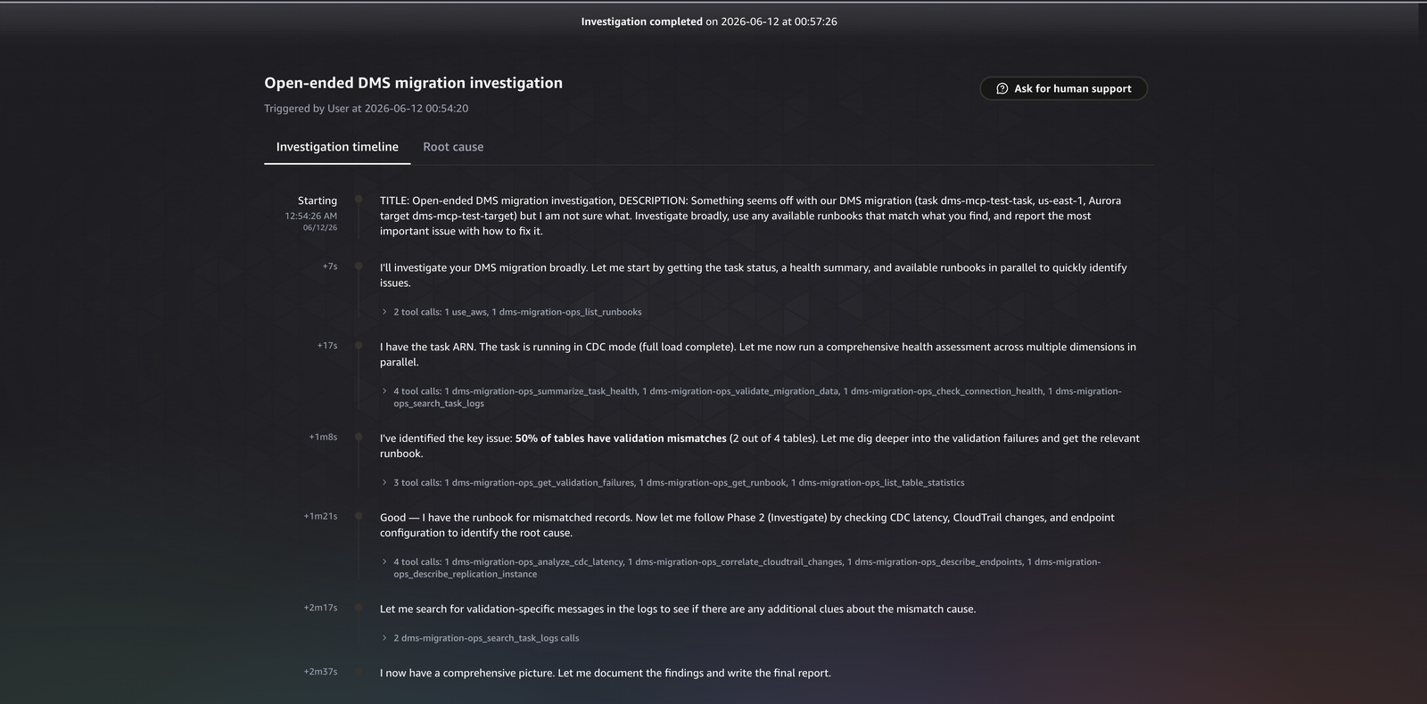
Something seems off with our DMS migration (task dms-mcp-test-task, us-east-1, Aurora target dms-mcp-test-target) but I am not sure what. Investigate broadly, use any available runbooks that match what you find, and report the most important issue with how to fix it.

Response

Given no specific symptom, the agent ran the broadest investigation of the suite: 12 distinct tools across 43 records. It swept the task status, validation state, connectivity, latency, replication instance, endpoints, and logs, then called list_runbooks, recognized the validation symptom it had found, and fetched get_runbook for the matching runbook, which returned the full procedure. It produced a finding about a datatype or precision difference in the MySQL to PostgreSQL migration and followed the runbook to the recommended remediation. In our test runs this broad sweep of twelve tools resolved to a single prioritized finding in a few minutes, against the open-ended manual triage it replaces, which has no fixed time because the operator does not yet know where to look. (Illustrative from our runs, not a benchmark.)

Tools the agent chose: validate_migration_data, get_validation_failures,
list_table_statistics, check_connection_health, describe_endpoints,
describe_replication_instance, analyze_cdc_latency, summarize_task_health,
search_task_logs, correlate_cloudtrail_changes, list_runbooks, get_runbook

Open-ended investigation

Figure 4. The open-ended investigation, showing the agent browse the runbook catalog and follow the matching runbook.

Post-Migration: Review stabilization and monitoring

After cutover, the question shifts from “did the data move” to “is the new database healthy and watched.”

Query

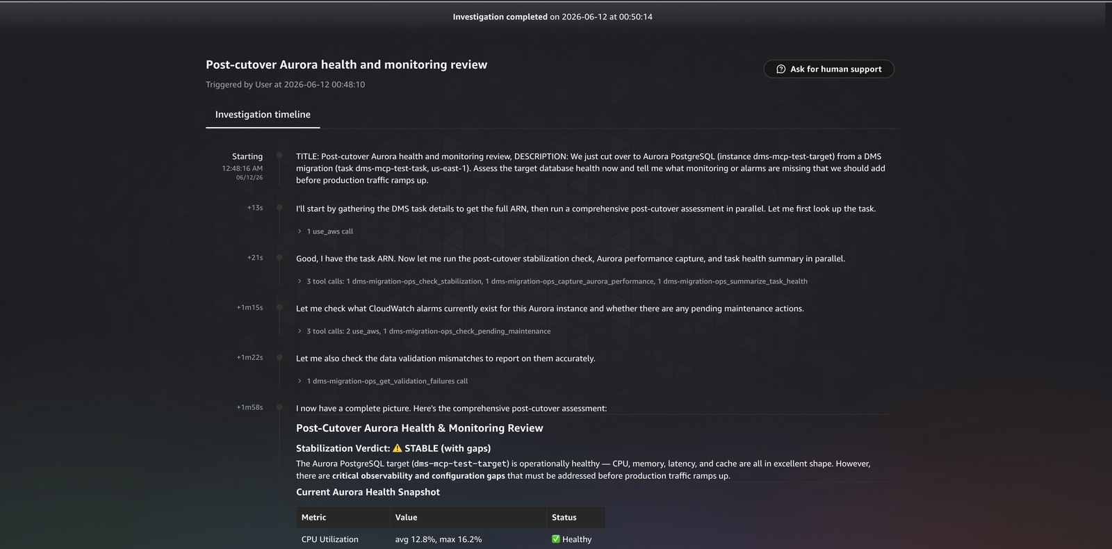
We just cut over to Aurora PostgreSQL (instance dms-mcp-test-target) from a DMS migration (task dms-mcp-test-task, us-east-1). Assess the target database health now and tell me what monitoring or alarms are missing that we should add before production traffic ramps up.

Response

The agent selected the stabilization tool set: check_stabilization, capture_aurora_performance, summarize_task_health, get_validation_failures, and check_pending_maintenance. It read the Aurora target health (CPU, connections, read and write latency, buffer cache hit ratio, and the top Performance Insights wait event), then assessed what monitoring was missing for a database about to take production traffic. The point of this phase is the interpretation: a buffer cache hit ratio that stays low after warmup points to missing indexes, and a new database with no alarm on connection count or query latency is one bad query away from an unmonitored outage. In our test runs the stabilization review returned target health and the specific missing alarms in about two minutes, versus manually inspecting Aurora metrics and Performance Insights and then deciding which alarms a freshly promoted database still lacks. (Illustrative from our runs, not a benchmark.)

Post-cutover stabilization review

Figure 5. The post-cutover stabilization review, with target health and the monitoring gaps the agent flagged.

Improve the agent with Skills and runbooks

A finding like the ValidationQueryCdcDelaySeconds race condition should improve the next migration, not be relearned. The agent’s migration judgment is captured in two places. DevOps Agent Skills are Markdown instruction sets that load automatically when relevant and tell the agent when to call a tool and how to read its output. The runbooks are fetched on demand: the agent calls list_runbooks to browse the catalog, then get_runbook to pull the procedure that matches what it found, as it did in scenario 5. You can fold each new finding back into a skill or runbook, so the agent improves with every migration.

To make the flywheel concrete, here is the runbook the agent fetched in the open-ended investigation. When it found the validation symptom, it called get_runbook and received this procedure, authored from earlier findings and grounded in public AWS documentation:

---
id: validation-mismatched-records
title: "Validation: mismatched records on a table"
severity: HIGH
triggers:
  - "ValidationState=Mismatched records"
  - "ValidationFailedRecords>0"
tools:
  - get_validation_failures
  - list_table_statistics
  - analyze_cdc_latency
  - correlate_cloudtrail_changes
---

# Validation: mismatched records on a table

A table shows Mismatched records, meaning source and target rows differ.
The row-level diffs are recorded in the awsdms_validation_failures_v1
control table on the target.

## Phase 1 — Assess
- Run get_validation_failures to see which tables are in Mismatched records
  and the failed-record counts.
- Run list_table_statistics to confirm the per-table validation state.

## Phase 2 — Investigate
- Query awsdms_validation_failures_v1 on the target for the failing rows/columns.
- Run analyze_cdc_latency: if validation runs during heavy CDC, transient
  diffs can appear while changes are in flight.
- Run correlate_cloudtrail_changes to check for an out-of-band write or reload.
- Check for data-type, precision, timezone, or character-set differences.

## Phase 3 — Report
- State which tables diverged and by how many records.
- Name the most likely cause (type/precision, timezone, encoding, out-of-band write).
- Recommend revalidating the table after the cause is corrected.

## Remediation (operator action)
- Correct the underlying difference, then revalidate with validate-only.

> All steps use read-only MCP tools. Remediation actions are operator tasks
> and are not performed by the tools.

The judgment for when to apply a runbook lives in a DevOps Agent Skill, a Markdown instruction set that loads automatically when relevant. The data-validation skill, for example, encodes the rules the agent follows before it draws a conclusion:

# Skill: DMS Data Validation Assessment

## Critical Rules
- Every finding MUST cite actual numbers from the metrics report, never generalize.
- Do NOT fabricate or estimate any metric. If data is missing, say "Data not available."
- Do NOT hardcode thresholds, use relative comparisons (% of total, trend direction).
- Validation metrics come from TWO sources: the DMS table-statistics API AND
  CloudWatch. Cross-reference both.

## Concepts to Evaluate — ValidationState machine
- Validated          = healthy, all rows confirmed matching
- Mismatched records = ACTION REQUIRED, source/target differ, check failure table
- Suspended records  = source churn too high, DMS cannot compare
- No primary key     = CANNOT VALIDATE, table lacks a PK
Flag if Mismatched + Suspended + Error tables exceed 5% of the total.

Every new finding folds back into a runbook or a skill, so the next migration starts from what the last one learned. The ValidationQueryCdcDelaySeconds race condition from scenario 2 becomes a trigger the agent recognizes on sight, rather than something it has to rediscover.

When to use this approach

This pattern fits issue investigation, pre-cutover readiness gates, and post-cutover stabilization reviews, where an operator hands the agent a symptom and wants a grounded root cause from read-only tools. It is not a replacement for continuous monitoring or alarms, and it does not ship logs for long-term retention. Use it alongside your existing CloudWatch alarms and dashboards, not instead of them.

Clean up

To avoid ongoing charges, delete the resources you created. Delete the CloudFormation stack with aws cloudformation delete-stack --stack-name dms-mcp-test-mcp-server. Remove the MCP server from your Agent Space and deregister it. If you provisioned a test migration with the repository scripts, run the included cleanup script.

Conclusion

Migration issues usually stem from operational problems, not data problems, and AWS DMS does not catch them. In this post, you saw how to extend AWS DevOps Agent to investigate them autonomously, using a sample MCP server that exposes read-only, migration-specific tools and runbooks. Across five real investigations, the agent chose the right tools for each question, found the affected tables, named the exact task setting behind a validation race condition, and followed a runbook to a fix. Because the tools are read-only and access is least-privilege IAM, you can give them to an autonomous agent without widening your operational scope.

To get started, deploy the MCP server from the GitHub repository, register it with your Agent Space, and turn on DMS data validation before your next cutover.

About the authors

Chitresh Saxena

Chitresh Saxena
Chitresh Saxena is a Senior AI/ML Specialist, specializing in generative AI solutions and dedicated to helping customers successfully adopt AI/ML on AWS. He excels at understanding customer needs and provides technical guidance to build, launch, and scale AI solutions that solve complex business problems.

Neel Sendas

Neel Sendas
Neel Sendas is a Principal Technical Account Manager at AWS, leading Cloud Operations for some of AWS’s largest enterprise customers across ML governance, cloud finance, and operational resilience at scale. He is also a core member of AWS’s Machine Learning Technical Field Community, helping shape the roadmap for AWS AI/ML services.

Tipu Qureshi

Tipu Qureshi
Tipu Qureshi is a Senior Principal Technologist in AWS Agentic AI, focusing on operational excellence and incident response automation. He works with AWS customers to design resilient, observable cloud applications and autonomous operational systems.

Hybrid cloud orchestration: Modernizing on-premises infrastructure management with AWS

2026-09-01 Sandeep Singh

Post Syndicated from Sandeep Singh original https://aws.amazon.com/blogs/architecture/hybrid-cloud-orchestration-modernizing-on-premises-infrastructure-management-with-aws/

This post demonstrates how to build a hybrid cloud orchestration solution that manages distributed on-premises infrastructure at scale using AWS serverless technologies. If you manage geographically dispersed data centers with thousands of servers that require bare-metal configuration, deployment, and ongoing lifecycle management, this solution provides centralized control while maintaining on-premises execution. Many of these environments also need the Kubernetes control plane itself to stay on-premises. This can be for data sovereignty, regulatory, or policy reasons, or because the network to AWS is disconnected, disrupted, intermittent, or limited (DDIL). Amazon EKS Anywhere runs the entire cluster on your own hardware, and this solution orchestrates it at scale from AWS. For on-premises workloads that can use a managed Amazon Elastic Kubernetes Service (Amazon EKS) control plane in the cloud, Amazon EKS Hybrid Nodes is the recommended approach.

In Part 1 of this series, you’ll learn the core architecture patterns for building an event-driven orchestration engine using AWS Lambda, AWS Step Functions, and Amazon DynamoDB. With this foundation, you can automate server lifecycle management through vendor-agnostic APIs, deploy EKS Anywhere clusters consistently across sites, and establish centralized observability for your entire infrastructure. In subsequent posts, we walk through the implementation with code examples, deployment templates, and detailed workflows for server and cluster management.

The challenge: Managing distributed on-premises infrastructure at scale

Managing distributed on-premises infrastructure at scale presents these challenges:

Inconsistency across locations: Different hardware vendors, network architectures, and compliance requirements lead sites to develop their own procedures. The same Kubernetes cluster deployment can produce different results at each site, such as the cluster version installed or the set of add-ons enabled. Without centralized orchestration, identical operations succeed at some locations but fail at others.

Manual lifecycle bottlenecks: The infrastructure lifecycle spans multiple layers requiring manual intervention. Hardware operations include BIOS configuration, firmware updates, and power management. OS operations cover installation and patching. Kubernetes operations encompass cluster creation, version upgrades, and scaling. Application operations involve deployment and maintenance. While manageable for individual servers, these processes become overwhelming bottlenecks when multiplied across thousands of geographically distributed machines.

Fragmented visibility: When management tools operate independently at each site, aggregating data across the entire environment becomes challenging. Operators struggle to answer enterprise-wide questions: How many servers are running outdated firmware? Which clusters are approaching capacity? Without centralized observability, identifying issues and planning capacity requires manual investigation across multiple locations.

Scalability limitations: Orchestration tools designed for a single data center encounter fundamental limitations at enterprise scale. Coordination mechanisms that work for dozens of servers fail when managing thousands. State synchronization becomes unreliable. Maintenance windows that are straightforward for a single site become logistical challenges across hundreds of locations.

Core technologies for hybrid orchestration

To address these operational challenges, four core technologies work together to deliver centralized orchestration with distributed execution:

Hybrid connectivity: Secure network connectivity between AWS and on-premises sites forms the foundation for centralized orchestration. AWS Direct Connect provides dedicated private connections, while AWS Site-to-Site VPN offers encrypted tunnels over the internet. This connectivity allows AWS services running in your virtual private cloud (VPC) to coordinate lifecycle operations with on-premises infrastructure.

AWS architecture stack: The AWS serverless stack along with Amazon EventBridge sets the foundation for an event-driven orchestration engine. Additional compute services include AWS CodeBuild for build processes, AWS Batch for long-running jobs, and AWS Systems Manager for on-premises tasks. These services provide a framework that can handle different execution runtimes while AWS manages the underlying infrastructure.

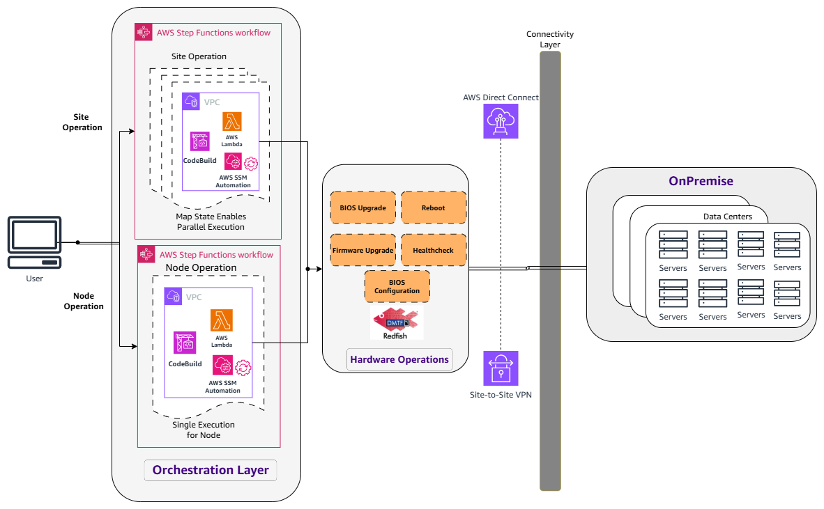
Redfish APIs: Redfish (a standard protocol for hardware management developed by the DMTF) delivers vendor-agnostic APIs for hardware management, allowing standardized control of bare-metal servers. Through Redfish, BIOS configuration, firmware updates, power management, and health monitoring operations are executed across diverse hardware environments.

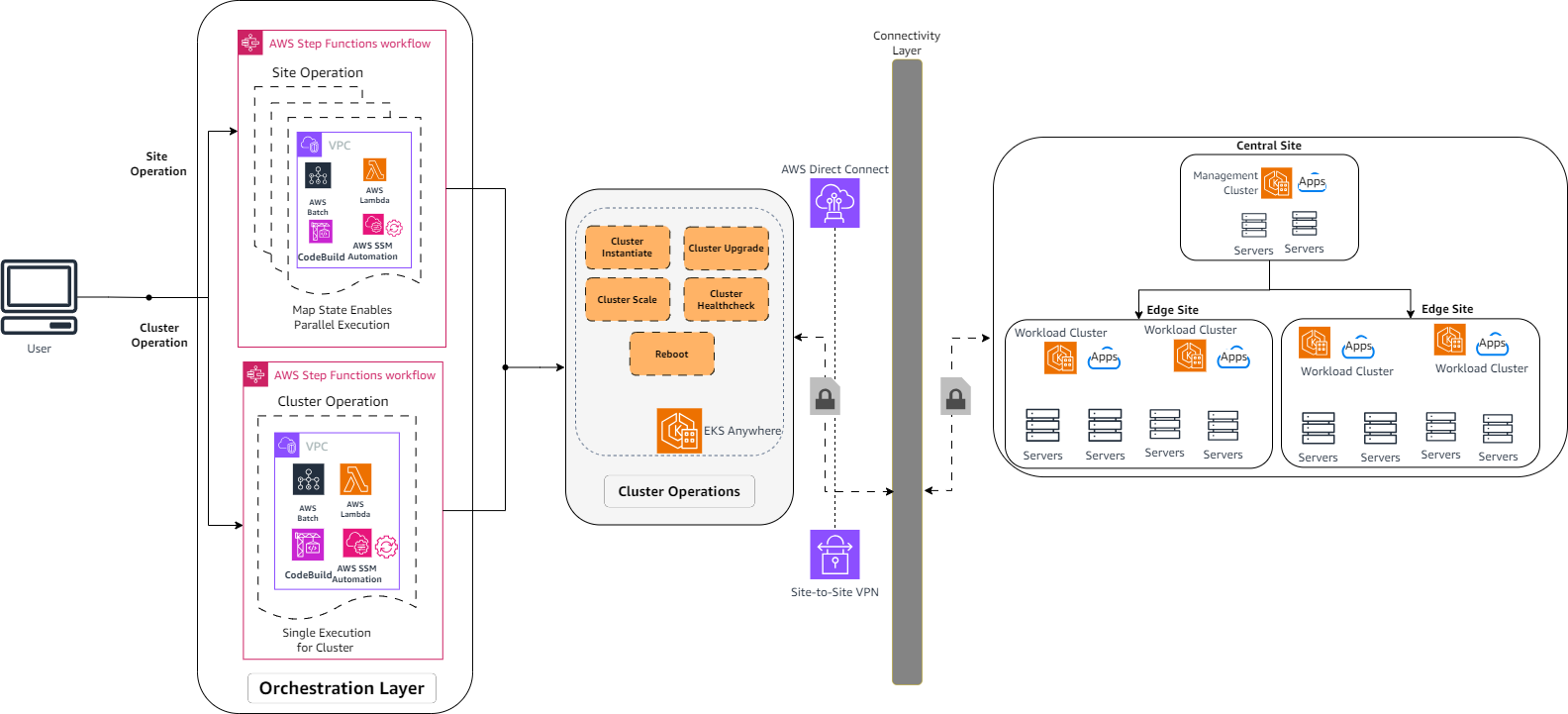
Amazon EKS Anywhere: EKS Anywhere creates and operates Kubernetes clusters on your own infrastructure, using the same Amazon EKS Distro that powers Amazon EKS in the cloud. It supports several infrastructure providers, including the bare-metal provider this solution uses. Cluster lifecycle operations and maintenance are your responsibility, which is the work the orchestration engine automates across sites. If you have on-premises or edge environments with reliable connectivity to an AWS Region, Amazon EKS Hybrid Nodes is the recommended alternative. For the full set of options, see Amazon EKS deployment options.

Architecture overview

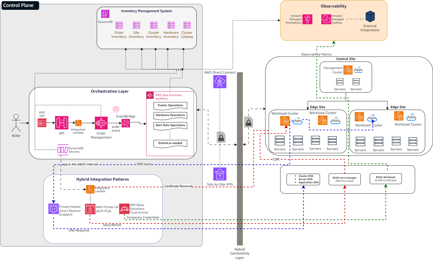
High-level architecture showing the AWS orchestration engine, on-premises EKS Anywhere clusters, and the hybrid connectivity linking them

Figure 1: High-level architecture of the hybrid cloud orchestration solution

The architecture consists of three primary layers: a centralized orchestration engine on AWS, distributed on-premises infrastructure running EKS Anywhere clusters, and hybrid connectivity linking the two environments. Serverless technologies coordinate lifecycle operations across hundreds of sites while maintaining comprehensive state tracking through an Inventory Management System.

Foundational concepts

The architecture is built on several foundational concepts that organize how resources are managed, and operations are coordinated.

Site: A physical location or logical grouping housing on-premises infrastructure. Sites provide an organizational framework for distributed operations, supporting location-specific policies, connectivity requirements, and compliance controls (for example, central, regional, or edge data centers).

Server: Bare-metal servers within sites that provide the physical compute, storage, and networking foundation for containerized workloads. Hardware resources are managed through vendor-agnostic Redfish APIs.

Cluster: EKS Anywhere Kubernetes clusters deployed on hardware resources, consisting of both management clusters (for orchestration operations) and workload clusters (for hosting applications).

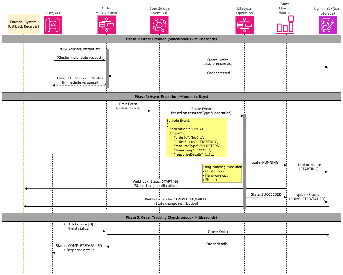
Order: A trackable infrastructure lifecycle operation that executes as a workflow. When an operator requests an action like rebooting all servers in a site, an order is created with a unique ID. This emits an event, which Amazon EventBridge routes to the corresponding AWS Step Functions workflow. Operators can monitor progress by checking the order status, which is updated in response to state-change events emitted by the running workflow.

Inventory Management System: Centralized state repository

The Inventory Management System is the central state repository, using DynamoDB tables to track infrastructure resources and their relationships across hundreds of distributed sites.

DynamoDB tables maintain information about sites, hardware, clusters, orders, and a catalog of reusable configurations. Sites organize resources by location, storing network configurations, gateway addresses, and regional information. Hardware inventory captures server configurations (BIOS and firmware versions, encrypted credentials), network details (IP addresses, MAC addresses), operational status, physical location (rack number, mounting position), and cluster membership. Clusters maintain Kubernetes configurations, node group details, addon versions, and relationships to management clusters. Orders track operation lifecycles from initiation through completion, capturing the operation type, target resources, execution status, and workflow outputs. The catalog stores vetted blueprints and templates that standardize deployments across the infrastructure.

As infrastructure changes occur, the inventory reflects the current state of resources and their dependencies, acting as the single source of truth for operational history and resource relationships.

Event-driven orchestration engine

With centralized state tracking using the Inventory Management System, the orchestration engine coordinates infrastructure operations through an API-driven framework built on AWS serverless technologies. This architecture delivers scalable, event-driven orchestration without operational overhead.

API layer

The API layer exposes a RESTful interface through Amazon API Gateway for create, read, update, and delete (CRUD) operations on infrastructure resources. A unified operator portal serves as the front end for this API, giving operators a self-service interface to perform lifecycle operations without requiring CLI or direct API knowledge. Lambda functions process incoming requests, validate parameters, and integrate with the order management system to initiate operations.

Orchestration layer

Step Functions executes specialized state machines that integrate with AWS services for compute, storage, and networking operations, providing retry logic, error handling, and state checkpointing.

Step Functions supports a callback pattern where a workflow can pause, hand off a task to an external system with a unique token and resume only when that system calls back with the token. This is critical for hybrid cloud orchestration because it allows workflows to pause execution and wait for external systems to signal completion. This capability addresses the challenge of coordinating AWS-based workflows with on-premises systems that may take hours to complete operations like firmware updates or cluster deployments. A workflow can hand off a task to on-premises infrastructure, pause, and resume only when the on-premises system reports back.

The Distributed Map state scales operations from individual resources to thousands across multiple sites. For example, a workflow that manages the power state of a single server can scale to manage power states across thousands of servers simultaneously.

Amazon EventBridge provides event-driven automation capabilities, triggering workflows based on infrastructure state changes. When inventory records are updated, Amazon EventBridge Rules evaluate the changes and invoke appropriate Step Functions workflows. This decouples components and supports reactive automation patterns, such as automatically scaling clusters when capacity thresholds are reached or starting maintenance workflows when hardware health checks fail.

Security and configuration

Security and configuration management are handled through multiple AWS services. AWS Systems Manager Parameter Store provides centralized configuration storage, while AWS Secrets Manager securely manages sensitive credentials and secrets. AWS Identity and Access Management (IAM) roles provide fine-grained access control across components, with IAM Roles Anywhere extending AWS access to on-premises clusters without requiring long-term credentials.

AWS Systems Manager hybrid activations register on-premises instances with AWS, allowing the Systems Manager agent to manage on-premises infrastructure alongside cloud resources. This delivers a unified management interface for configuration, patching, and command execution across both environments.

AWS Private Certificate Authority manages certificates for secure communications between orchestration components and on-premises infrastructure. Each component operates with least-privilege permissions, accessing only the resources required for its specific function.

Order management: Coordinating operations at scale

Order management flow where an API request maps through Amazon EventBridge rules to Step Functions workflows and updates order status in DynamoDB

Figure 2: Order management flow from API request to workflow execution

The orchestration engine coordinates operations through an order management system built on Amazon EventBridge rules that map API operations to Step Functions workflows. When an API request initiates an operation like `/clusters/{id}/terminate`, an Amazon EventBridge Rule routes the request to the corresponding workflow based on the resource and operation type. The system creates a record in DynamoDB and returns an order ID immediately, while the workflow executes asynchronously.

This event-driven system listens and responds to events throughout the operation lifecycle. As workflows execute, AWS-managed events from Step Functions and custom events from workflow logic progressively update the order status in DynamoDB. This allows operators to initiate operations without waiting for completion, which may take minutes to hours depending on the complexity of the operation.

The following core capabilities are enabled by order management:

Order lifecycle tracking: Operators can query order status through the API to monitor progress and track the complete audit trail from creation through execution to completion or failure.

Callback support: Orders support callbacks to both other workflows and external webhooks. Workflows can trigger other workflows upon completion, while webhook endpoints receive notifications upon state changes or completion. This supports integration with external systems such as ticketing platforms, notification services, or custom dashboards.

Conflict management: Integration with the inventory system prevents conflicting operations by denying new orders if another one is running on the same resource, preventing scenarios like cluster scaling during an upgrade.

Extensibility: New resource types and operations can be added by implementing Step Functions workflows and registering Amazon EventBridge rules that map API endpoints to workflows. The core order tracking logic remains unchanged.

Lifecycle management framework

The lifecycle management framework addresses two primary resource types, each with distinct operational requirements: bare-metal hardware and Kubernetes clusters.

Hardware management

Hardware lifecycle management flow using vendor-agnostic Redfish APIs to run firmware, power, and BIOS operations across on-premises servers

Figure 3: Hardware lifecycle management across distributed sites

The solution provides hardware lifecycle management across distributed on-premises sites through a vendor-agnostic approach integrated with the Inventory Management System.

Supported hardware lifecycle operations

Firmware management: Automated updates and configuration management.
NIC upgrades: Network interface card firmware updates.
Power management: Remote reboot, shutdown, and power cycling.
Health: Processor, memory, and disk health checks.
BIOS configuration: Define and apply specific golden templates.

This approach automates traditional manual hardware management, so operations can efficiently handle hundreds of servers across multiple distributed sites.

Cluster management

Cluster lifecycle management flow where the orchestration engine assembles a configuration file and hardware inventory and runs EKS Anywhere commands through Systems Manager and Batch

Figure 4: EKS Anywhere cluster lifecycle management across sites

Cluster management uses Amazon EKS Anywhere for consistent Kubernetes operations across sites. To create a cluster from bare metal servers, a configuration file and a hardware inventory CSV that lists the servers and their network details are prepared and passed to the EKS Anywhere CLI, which network boots them, installs the operating system and Kubernetes, and brings up the cluster. For the full set of steps and configuration options, see the EKS Anywhere bare metal documentation.

EKS Anywhere supports two cluster types:

Management: Dedicated clusters that host orchestration components to manage the lifecycle of workload clusters.
Workload: Application-hosting clusters managed by their corresponding management cluster.

This mapping of management to workload clusters is maintained in the Inventory Management System to give a unified view of cluster distribution across the infrastructure. When an operator requests a cluster through the API, the orchestration engine assembles the required inputs: the configuration file comes from a blueprint in the Cluster Catalog, and the hardware CSV comes from the servers recorded in the Inventory Management System. A workflow then runs the EKS Anywhere commands through Systems Manager (SSM) and Batch, which execute them against the on-premises servers.

Scalable operations

Cluster operations must execute in the proper sequence across the distributed environment, handling dependencies between clusters and their components. For instance, cluster creation begins with hardware selection based on placement strategy, pre-flight checks, bootstrapping an Admin machine, executing on-premises commands and awaiting completion, add-ons installation, and post-deployment health checks. The orchestration engine handles this using Step Functions with child workflows, callback patterns, and dependency mapping.

Supported cluster lifecycle operations

Cluster creation: Automated provisioning of management and workload clusters with customizable configurations.
Cluster scaling: Dynamic addition or removal of worker nodes based on capacity requirements.
Cluster upgrades: Coordinated Kubernetes version upgrades with minimal disruption.
Cluster termination: Graceful cluster decommissioning with proper resource cleanup.

These automated workflows reduce the operational complexity of managing Kubernetes at scale and support consistent cluster operations from edge locations to central data centers.

Monitoring and observability

Managing geographically distributed infrastructure requires centralized observability since operators often need to investigate issues across individual sites, correlating data from different hardware vendors and software layers.

This solution addresses the fragmented visibility challenge by aggregating telemetry from on-premises clusters into managed AWS services. AWS Distro for OpenTelemetry (ADOT), deployed as a collector on each EKS Anywhere cluster, scrapes and forwards metrics from the server, Kubernetes, and application layers to Amazon Managed Service for Prometheus in the AWS Region. Amazon Managed Grafana then provides unified dashboards and alerting across the entire distributed environment.

With this approach, operators can monitor server availability (through Redfish events or Prometheus node-exporter), Kubernetes cluster health (through kube-state-metrics), and application-level metrics from one place, regardless of the underlying hardware vendor.

For a detailed implementation walkthrough, including Redfish event subscription patterns, OpenTelemetry collector configuration, Prometheus alerting rules, and Grafana dashboard setup for distributed sites on EKS Anywhere, see our related post: Building observability on Amazon Managed Grafana built on EKS Anywhere.

Hybrid integration patterns

Although EKS Anywhere clusters run on-premises, applications on them can depend on capabilities that span the cloud boundary: DNS resolution across both environments, TLS certificates, access to AWS APIs, and persistent storage. AWS offers services designed for this hybrid integration, and the orchestration engine can apply them automatically from its inventory as clusters and applications change.

Automated DNS management

When the state of a cluster, server, or application changes, Amazon DynamoDB Streams automatically trigger Lambda functions that update DNS records in Amazon Route 53 private hosted zones. Route 53 Resolver endpoints make these records resolvable from both AWS and on-premises, which supports service discovery without manual DNS configuration.

Certificate lifecycle operations

AWS Private Certificate Authority acts as a managed CA for the clusters, so there is no need to run a certificate authority at each site. cert-manager and the AWS Private CA Issuer request, renew, and distribute certificates from it automatically, which helps avoid outages from expired certificates.

Secure AWS access

Workloads on the clusters often need to call AWS APIs, such as sending Fluent Bit logs to Amazon Simple Storage Service (Amazon S3), publishing metrics to Amazon Managed Service for Prometheus, or pulling images from Amazon Elastic Container Registry (Amazon ECR). AWS IAM Roles Anywhere issues short-lived AWS credentials in exchange for a certificate the workload already holds, so no long-lived keys are stored at each site. It accepts that certificate only if it chains to a trusted source, so the orchestration engine registers each cluster’s own CA certificate as its trust anchor when the cluster comes up.

Persistent storage integration

External storage solutions such as Portworx can be integrated for stateful applications. DynamoDB Streams trigger automated interactions with storage provider APIs during node provisioning and cleanup operations and perform the configuration and reclaiming of storage resources.

The event-driven approach makes it possible for dependent infrastructure components to remain synchronized with the actual state of clusters and hardware, reducing operational overhead and minimizing configuration drift.

Conclusion

This blog post explores the architecture and capabilities of the hybrid cloud orchestration solution that modernizes on-premises infrastructure management using AWS technologies and EKS Anywhere. We’ve demonstrated how you can build a scalable, event-driven orchestration engine that manages your distributed infrastructure across hundreds of sites while maintaining operational consistency.

What’s next

In this post series, we’ve focused on the architectural patterns and capabilities that enable enterprise-scale hybrid cloud orchestration. To get started today, review the Amazon EKS Anywhere documentation and set up a bare-metal cluster or use the Docker provider for development and testing. In Part 2, we walk through the implementation of the orchestration solution with infrastructure-as-code templates, Step Functions workflow definitions, and operational runbooks you can adapt to your environment. Follow the AWS Containers blog for the next installment.

About the authors

Build your own continuous modernization pipeline with AWS Transform custom

2026-08-28 Janardhan Molumuri

Post Syndicated from Janardhan Molumuri original https://aws.amazon.com/blogs/devops/build-your-own-continuous-modernization-pipeline-with-aws-transform-custom/

Introduction

Development velocity has reached new heights with AI-driven development tools and practices. Organizations are generating code faster than ever before. But that speed carries risk. Researchers Anderson, Parker, and Tan warned in MIT Sloan Management Review, “Legacy systems tend to carry hidden debt; layering AI-generated code on top of them creates additional tangled dependencies.” The faster you generate code, the faster technical debt compounds — especially in brownfield environments where outdated frameworks, deprecated libraries, and undocumented services already carry years of accumulated risk.

As organizations accelerate their software development, manual or periodic processes to synchronize dependencies and update documentation no longer keep pace, and technical debt piles up faster than ever. Continuous modernization built into your pipeline enables you to maintain up-to-date dependencies and documentation across repositories on every commit, preventing future tech debt and improving AI agent accuracy and accountability.“

You can embed AI-powered code transformations directly into your CI/CD pipelines, turning modernization from a periodic project into an automated, ongoing practice. AWS gives you two ways to get there. AWS Transform – continuous modernization is the fully managed option, delivering continuous modernization automatically with no pipeline for you to build or maintain. The Do-It-Yourself (DIY) approach assembles the same practices yourself using AWS Transform custom and your existing CI/CD platform. Choose DIY when you need to fit modernization into a specific pipeline (GitHub Actions, AWS CodePipeline, Jenkins, GitLab CI, and so on), or want to customize the workflow with existing tools like Dependabot.

In this post, we cover the DIY approach on how to set up a continuous modernization pipeline using AWS Transform custom and demonstrate it in action.

The Do It Yourself (DIY) path – continuous modernization pipeline with AWS Transform custom

Sample application: instrumentShop

For this walkthrough, we use a dated Java application called instrumentShop (Figure 1) — a Java microservices application built with Spring Boot that simulates an online instrument shop to demonstrate four practices: automated dependency remediation, auto-documentation on every commit, scaling transformations across repositories, and continual learning.

Architecture overview

Figure 1: instrumentShop Java application architecture

The instrumentShop application is a Spring Boot microservices application with a Spring Gateway (v1.5.19) routing traffic from a single HTTP/8010 entry point to four REST services: Agents, Instruments, Consumers, and Products. A Thymeleaf client provides server-side rendering, PostgreSQL 13.1 handles persistence via JDBC, and Hystrix provides circuit-breaking for inter-service calls. A ShopTester utility generates HTTP traffic for testing.

This application is a strong candidate for continuous modernization:

Spring Boot 1.5.19 is years past end of life and carries known CVEs
Hystrix has been in maintenance mode since Netflix deprecated it in 2018
Cross-service coordination — dependency updates must propagate across multiple microservices
Transitive dependency risk — PostgreSQL JDBC drivers and other transitive dependencies accumulate security advisories over time

A typical workflow for the continuous modernization pipeline is shown below (Figure 2):

A developer pushes code to main — GitHub Actions triggers the auto-documentation workflow, generating updated architecture docs and technical debt reports.
Dependabot detects a vulnerable dependency — A PR opens automatically. GitHub Actions triggers the dependency remediation workflow, runs AWS Transform custom to remediate the code, validates with tests, and pushes the result back to the PR.
A platform team defines a new transformation (e.g., “Upgrade Spring Boot to the latest stable release “) — The scheduled GitHub Actions workflow runs the transformation weekly in non-interactive mode across all instrumentShop microservices and other repositories in the portfolio.
The agent learns — Knowledge items from each execution improve future runs, reducing manual intervention over time.

Figure 2: AWS Transform continuous code modernization workflow

Prerequisites

Before setting up the continuous modernization pipeline, ensure you have the following:
An active AWS account with permissions for AWS Transform custom
AWS Transform CLI installed and configured in your development environment
Authentication with AWS credentials configured locally and proper IAM permissions to call AWS Transform
Git installed for cloning sample repositories
GitHub Dependabot enabled on your repository for automated vulnerability detection

Continuous modernization through CI/CD in action

Continuous modernization shifts code transformation from a periodic project into an automated, pipeline-driven practice. Instead of scheduling a “modernization sprint” once a year, your CI/CD pipeline identifies and remediates technical debt on every commit, every dependency alert, and across every repository.

We implement this through four practices, each powered by AWS Transform custom running as a step in GitHub Actions workflows.

Note: This post uses GitHub Actions because the instrumentShop demo repository is built with it. The same AWS Transform CLI (atx) commands work with AWS CodePipeline, Jenkins, GitLab CI, CircleCI, or any CI/CD system that runs shell commands. Continuous modernization is a practice, not a tool choice.

Important: Every atx custom def exec invocation in this post uses the –trust-all-tools flag, which allows the agent to execute tools without interactive confirmation. This is required for non-interactive CI/CD execution. Review your organization’s security policies before enabling this flag in production pipelines.

1. Dependency analysis and remediation

GitHub Dependabot scans your repository for known vulnerabilities and generates alerts when a new vulnerability is added or your dependency graph changes—for example, when you push commits that update packages or versions. However, resolving these alerts requires more than bumping a version number. Upgrading a dependency can introduce breaking API changes, require code modifications, or demand configuration updates.

AWS Transform custom helps handle the code changes needed to resolve the alerts. It runs via a GitHub Actions workflow that triggers automatically to:

Fetch the list of latest Dependabot alerts
Run AWS Transform custom to analyze the alerts and apply code transformations
Run your build and test suite to validate the changes
Create a new pull request for each resolved alert

The workflow calls a shell script that invokes the AWS Transform CLI in headless mode with retry logic. Place this script at the root of your repository:

run_dependabot_alert_fixes.sh:

#!/usr/bin/env bash
set -euo pipefail

# -------------------------------------------------------------------
# run_dependabot_alert_fixes.sh
# Runs the Dependabot alert remediation transformation in headless mode.
# Retries up to MAX_RETRIES times on failure.
#
# Usage:
#   ./run_dependabot_alert_fixes.sh [-n <transformation-name>] [-p <path>] [-c <build-command>]
#
# Defaults:
#   -n  Remediate-Critical-GitHub-Dependabot-Alerts-Java-Maven
#   -p  .                   (current directory)
#   -c  mvn clean install   (Maven build)
# -------------------------------------------------------------------

TRANSFORMATION_NAME="Remediate-Critical-GitHub-Dependabot-Alerts-Java-Maven"
CODE_PATH="."
BUILD_CMD="mvn clean install"
MAX_RETRIES=3

while getopts "n:p:c:" opt; do
  case $opt in
    n) TRANSFORMATION_NAME="$OPTARG" ;;
    p) CODE_PATH="$OPTARG" ;;
    c) BUILD_CMD="$OPTARG" ;;
    *) echo "Usage: $0 [-n <transformation-name>] [-p <path>] [-c <build-command>]" && exit 1 ;;
  esac
done

echo "=== AWS Transform Custom ==="
echo "Transformation: $TRANSFORMATION_NAME"
echo "Code path:      $CODE_PATH"
echo "Build command:  $BUILD_CMD"
echo "============================"

attempt=1
while [ $attempt -le $MAX_RETRIES ]; do
  echo "--- Attempt $attempt of $MAX_RETRIES ---"

  if atx custom def exec \
    -n "$TRANSFORMATION_NAME" \
    -p "$CODE_PATH" \
    -c "$BUILD_CMD" \
    -x -t; then
    echo "=== Transformation completed successfully ==="
    exit 0
  fi

  echo "Attempt $attempt failed."
  attempt=$((attempt + 1))

  if [ $attempt -le $MAX_RETRIES ]; then
    echo "Retrying in 10 seconds..."
    sleep 10
  fi
done

echo "=== All $MAX_RETRIES attempts failed ==="
exit 1

This script accepts optional flags to override the transformation name (-n), code path (-p), and build command (-c). The -x flag enables non-interactive mode and -t enables --trust-all-tools, both required for CI/CD execution. On failure, it retries up to three times with a 10-second backoff.

Your CI/CD workflow must configure AWS credentials and install the AWS Transform CLI before invoking this script. With this setup, Dependabot alerts are reviewed continuously for any changes — not just a version bump, but the complete code adaptation required to make the upgrade work.

2. Auto documentation

Documentation is one of the most neglected aspects of modern software development. Documentation increases accuracy and acts as a contract between requirements and implementation. AWS Transform custom codebase analysis capability generates structured documentation covering architecture, technical debt, code metrics, and migration planning on every incremental update ensuring every Agent or human that modifies the codebase is working from a true “current state”.

By embedding this as a post-push step in your CI/CD pipeline, your documentation stays current automatically. The workflow triggers on every pull request to main, runs your build and test suite, then calls a shell script that invokes AWS Transform custom to generate documentation and commits it back to the PR branch.

Place this script at the root of your repository:

run_code_analysis.sh:

#!/usr/bin/env bash
set -euo pipefail

# -------------------------------------------------------------------
# run_code_analysis.sh
# Runs an AWS Transform custom transformation in headless mode.
# Retries up to MAX_RETRIES times on failure.
#
# Usage:
#   ./run_code_analysis.sh [-n <name>] [-p <path>] [-c <build-cmd>] [-U <pr-url>]
#
# Defaults:
#   -n  GitHub-PR-Context-Codebase-Analysis
#   -p  .                   (current directory)
#   -c  mvn clean install   (Maven build)
#   -U  (empty)             PR URL
# -------------------------------------------------------------------

TRANSFORMATION_NAME="GitHub-PR-Context-Codebase-Analysis"
CODE_PATH="."
BUILD_CMD="mvn clean install"
PR_URL=""
MAX_RETRIES=3

while getopts "n:p:c:U:" opt; do
  case $opt in
    n) TRANSFORMATION_NAME="$OPTARG" ;;
    p) CODE_PATH="$OPTARG" ;;
    c) BUILD_CMD="$OPTARG" ;;
    U) PR_URL="$OPTARG" ;;
    *) echo "Usage: $0 [-n <name>] [-p <path>] [-c <build-cmd>] [-U <pr-url>]" && exit 1 ;;
  esac
done

echo "=== AWS Transform Custom ==="
echo "Transformation: $TRANSFORMATION_NAME"
echo "Code path:      $CODE_PATH"
echo "Build command:  $BUILD_CMD"
echo "PR URL:         $PR_URL"
echo "============================"

attempt=1
while [ $attempt -le $MAX_RETRIES ]; do
  echo "--- Attempt $attempt of $MAX_RETRIES ---"

  if atx custom def exec \
    -n "$TRANSFORMATION_NAME" \
    -p "$CODE_PATH" \
    -c "$BUILD_CMD" \
    -g "additionalPlanContext=$PR_URL" \
    -x -t; then
    echo "=== Transformation completed successfully ==="
    exit 0
  fi

  echo "Attempt $attempt failed."
  attempt=$((attempt + 1))

  if [ $attempt -le $MAX_RETRIES ]; then
    echo "Retrying in 10 seconds..."
    sleep 10
  fi
done

echo "=== All $MAX_RETRIES attempts failed ==="
exit 1

This script accepts optional flags for the transformation name (-n), code path (-p), build command (-c), and PR URL (-U). Pass the PR URL to the agent via the -g flag as additionalPlanContext, giving it awareness of the pull request context when generating documentation. On failure, it retries up to three times with a 10-second backoff.

Your CI/CD workflow must configure AWS credentials and install the AWS Transform CLI before invoking this script. The workflow commits the generated documentation back to the PR branch automatically, keeping your architecture docs and technical debt reports current with every code change.

Every push now updates the documentation (Figures 3 and 4) — reducing knowledge silos and preserving institutional knowledge.

A GitHub pull request triggering the auto-documentation workflow.

Figure 3: PR triggering auto-documentation

Generated documentation output showing architecture and technical debt reports.

Figure 4 – Generated documentation output

3. Scale across repositories

For organizations with hundreds of microservices, transforming one repository at a time doesn’t scale. AWS Transform custom non-interactive mode combined with GitHub Actions matrix strategy allows you to orchestrate transformations across your entire portfolio in parallel. You can run them on demand or on a recurring schedule, so modernization runs as a continuous practice rather than a one-time project.

# .github/workflows/scale-modernization.yml
name: Scale Modernization
on:
  schedule:
    - cron: '0 6 * * 1'
  workflow_dispatch:

jobs:
  transform-repos:
    runs-on: ubuntu-latest
    strategy:
      matrix:
        repo:
          - magnefique-studios/instrumentShop
          - magnefique-studios/orderService
          - magnefique-studios/paymentGateway
    steps:
      - name: Checkout ${{ matrix.repo }}
        uses: actions/checkout@v4
        with:
          repository: ${{ matrix.repo }}
          token: ${{ secrets.GH_PAT }}

      - name: Configure AWS credentials
        uses: aws-actions/configure-aws-credentials@v4
        with:
          role-to-assume: ${{ secrets.AWS_ROLE_ARN }}
          aws-region: us-east-1

      - name: Install ATX CLI
        run: curl -fsSL https://transform-cli.awsstatic.com/install.sh | bash

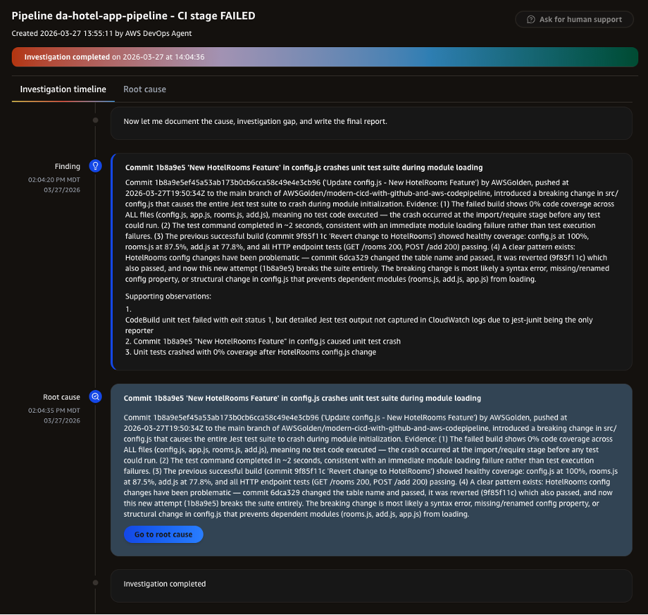
      - name: Run transformation
        run: |
          atx custom def exec \
            --transformation-name "spring-boot-3-upgrade" \
            --code-repository-path "." \
            --build-command "mvn clean install" \
            --non-interactive \
            --trust-all-tools

Tip: GitHub Actions matrix strategy runs each repository in parallel automatically — no separate orchestration layer needed. For larger portfolios, you can also wrap this in AWS Batch or AWS Fargate for large-scale parallel execution. The AWS Transform web console tracks progress across all repositories in a single view.

4. Continual learning

Each time AWS Transform custom completes a transformation, a memory agent scans the full execution trajectory and extracts lessons. Lessons include patterns that the agent learned, decisions that the agent made during planning, and feedback you provide during execution. AWS Transform custom automatically attaches these lessons to your transformation definition, which improves accuracy in subsequent runs.

AWS Transform custom applies lessons automatically, and each lesson belongs to a category that groups related lessons for review. You can browse and archive any lesson you do not want AWS Transform custom to apply to future runs.This keeps a human in the loop on what the agent “remembers” which matters when the same transformation runs across many repositories with different conventions.

In practice, this means your “Spring Boot 3 Upgrade” transformation gets sharper with each execution. The first repository surfaces the edge cases; once you review the resulting lessons and archive the ones that do not fit, subsequent runs handle those edge cases without intervention.

For production use, you can combine these practices into a single workflow file:

Note: The individual workflows shown in Practices 1–3 are presented separately for clarity. Combine them into a single workflow file as shown here, or keep them as separate workflow files depending on your team’s preference.

# .github/workflows/continuous-modernization.yml
name: Continuous Modernization
on:
  push:
    branches: [main]
  pull_request:
    types: [opened]
  schedule:
    - cron: '0 6 * * 1'

jobs:
  dependency-remediation:
    if: github.actor == 'dependabot[bot]'
    runs-on: ubuntu-latest
    steps:
      - uses: actions/checkout@v4
        with:
          ref: ${{ github.head_ref }}
      - name: Configure AWS credentials
        uses: aws-actions/configure-aws-credentials@v4
        with:
          role-to-assume: ${{ secrets.AWS_ROLE_ARN }}
          aws-region: us-east-1
      - name: Install ATX CLI
        run: curl -fsSL https://transform-cli.awsstatic.com/install.sh | bash
      - name: Remediate dependency changes
        run: |
          atx custom def exec \
            --transformation-name "dependency-remediation" \
            --code-repository-path "." \
            --build-command "mvn clean install" \
            --non-interactive \
            --trust-all-tools

  auto-documentation:
    if: github.event_name == 'push'
    runs-on: ubuntu-latest
    steps:
      - uses: actions/checkout@v4
      - name: Configure AWS credentials
        uses: aws-actions/configure-aws-credentials@v4
        with:
          role-to-assume: ${{ secrets.AWS_ROLE_ARN }}
          aws-region: us-east-1
      - name: Install ATX CLI
        run: curl -fsSL https://transform-cli.awsstatic.com/install.sh | bash
      - name: Generate documentation
        run: |
          atx custom def exec \
            --transformation-name "codebase-documentation" \
            --code-repository-path "." \
            --build-command "echo 'docs-only'" \
            --non-interactive \
            --trust-all-tools

  weekly-modernization:
    if: github.event_name == 'schedule'
    runs-on: ubuntu-latest
    steps:
      - uses: actions/checkout@v4
      - name: Configure AWS credentials
        uses: aws-actions/configure-aws-credentials@v4
        with:
          role-to-assume: ${{ secrets.AWS_ROLE_ARN }}
          aws-region: us-east-1
      - name: Install ATX CLI
        run: curl -fsSL https://transform-cli.awsstatic.com/install.sh | bash
      - name: Run modernization scan
        run: |
          atx custom def exec \
            --transformation-name "tech-debt-analysis" \
            --code-repository-path "." \
            --build-command "mvn clean install" \
            --non-interactive \
            --trust-all-tools

Conclusion

Continuous modernization moves code transformation out of periodic sprints and into your CI/CD pipeline. By combining GitHub Dependabot’s vulnerability detection with AWS Transform custom agent, orchestrated through GitHub Actions, you can:

Remediate dependency vulnerabilities automatically — beyond version bumps to full code adaptation
Keep documentation current with every commit, preserving institutional knowledge
Scale transformations across hundreds of repositories with consistent quality
Improve continuously as the agent accumulates knowledge items from each execution

The instrumentShop sample application demonstrates that even a moderately complex microservices architecture — with end-of-life Spring Boot versions, deprecated libraries like Hystrix, and multiple interconnected services — can be continuously modernized without dedicated modernization sprints.

Ready to get started? This post walked through the do-it-yourself path with AWS Transform custom. If you would rather have continuous modernization delivered as a fully managed service, explore AWS Transform continuous modernization. Either way, visit the AWS Transform documentation to start your continuous modernization journey.

Closing the AI agent trust gap with graduated autonomy

2026-08-26 Dev Arora

Post Syndicated from Dev Arora original https://aws.amazon.com/blogs/architecture/closing-the-ai-agent-trust-gap-with-graduated-autonomy/

How much to trust an AI agent is now a daily operational question. Agents read customer data, open tickets, process refunds, and delete accounts, yet most teams pick up a binary: full access or read-only. Full access is risky because agents fail unpredictably. Read-only leaves most of the agent’s value unused. The distance between what an agent could do and what an operator trusts it to do is the agent’s trust gap.

In this post, we describe graduated autonomy, an architectural pattern that closes the gap. Agents earn expanded permissions through sustained reliability and lose them when performance degrades. Amazon Bedrock AgentCore, a platform to build, connect, and optimize agents at scale with any framework or model, provides the runtime, gateway, policy, and evaluation capabilities. Amazon DynamoDB stores trust state. AWS CodePipeline gates delivery on evaluation results. We cover each layer’s responsibility and the key design decision behind it.

The agent trust gap

Identity and access management answers “who can do what?” once, at provisioning. That model assumes that the principal behaves consistently. A large language model agent breaks it: the same agent can be accurate Monday and hallucinated Tuesday after a prompt change or model update.

Closing the gap requires three capabilities raw API logs rarely provide:

Visibility. API logs tell engineers what happened but tell a compliance officer nothing about whether an action was safe.
Decision provenance. Tracing an action back to the signal that triggered it, the alternatives considered, and the confidence held.
Reversibility. Pre-action state capture, so operators can recover from incorrect actions.

The framework that implements this pattern delivers all three through six architectural layers.

Solution overview

The six layers:

Scoring engine computes trust from configurable dimensions.
Tier system translates sustained scores into autonomy levels.
Pre-execution layer blocks dangerous actions before they run.
Enforcement layer applies tiers through Cedar policies at the infrastructure level.
Post-execution layer evaluates outcomes, records of provenance, and feeds signals back to scoring.
Delivery gate keeps degraded agent versions out of production.

Architecture diagram of the trust framework as a clockwise closed loop: the scoring engine produces a weighted trust score from five dimensions, the tier system converts sustained scores into autonomy tiers T1 through T4, the pre-execution and enforcement layers apply the current tier through in-process checks and Cedar policies, and the post-execution layer returns outcome scores, honeypot results, and human overrides to the scoring engine, with an audit trail at the center recording every decision.

Figure 1: The trust framework’s closed loop.

Each layer is replaceable: the scoring model, tier thresholds, pre-execution signals, and evaluation criteria are configuration, not code. Each layer also embodies one deliberate design decision, developed in the following sections:

Layer	Key design decision
Scoring engine	Safety is an independent floor, never averaged away by strong metrics
Tier system	Start every agent at T1. Promote slowly, demote immediately
Pre-execution layer	Fast in-process filters are backstopped, never solely trusted
Enforcement layer	Deny by default, enforced outside the agent’s process
Post-execution layer	Audit records capture pre-action state, making recovery possible
Delivery gate	One unauthorized tool call in adversarial tests blocks release

The scoring engine

The scoring engine computes a weighted score from 0 to 100 per agent over a rolling window of 50 actions, from five dimensions:

Dimension	Weight	What it measures
Accuracy	25%	Task completion correctness against expected outcomes
Safety	20%	Boundary respect, adversarial content detection, permitted tool adherence
Consistency	20%	Behavioral predictability, inverse of tool-use pattern drift
Compliance	20%	Reasoning quality before acting, guardrail adherence
Efficiency	15%	Execution without unnecessary retries or resource waste

The composite drives dashboards and tier assignment, but safety acts as an independent floor, so a dangerous individual metric never hides strength elsewhere.

The tier system

Every new agent starts at T1, regardless of test performance:

Tier	Score range	Permissions
T1: Probation	0 to 40	Read and list only. Two tools visible.
T2: Supervised	41 to 70	Add write operations. Human approves high-risk.
T3: Trusted	71 to 90	Execute and modify. Anomalies flagged for review.
T4: Autonomous	91 to 100	Full access. Post-hoc audit only.

Three rules govern transitions:

Promotion requires sustained performance. The score must stay above the promotion threshold for the entire rolling window.
Demotion is immediate. When safety drops below its floor or injection is detected, the agent moves down.
Hysteresis prevents oscillation. Promotion into a tier requires a score 5 points above that tier range floor. Demotion happens at the range floor itself. An agent at a boundary cannot flap between tiers.

Trust state lives in Amazon DynamoDB as a current state record plus a time-series history per agent. Enforcement components read the current tier on every invocation, a lookup DynamoDB typically serves in single-digit milliseconds.

The pre-execution layer

Post-execution evaluation cannot undo damage, so the pre-execution layer evaluates every tool’s call and can block it before execution. It scores six signals independently:

Adversarial injection detection. Pattern matching against known injection phrases. One match triggers an instant block and a trust penalty.
Sensitive target detection. Regex matching credentials, tokens, and private keys in tool arguments.
Dangerous tool detection. Flagging tools that match destructive operation patterns.
Behavioral consistency. Comparing the current tool call against the agent’s historical tool-use distribution.
Confidence calibration. Comparing stated confidence against historical accuracy. Overconfident failures are penalized at twice the normal rate.
Reasoning quality. Checking whether the agent provided reasoning before acting.

These checks are fast first-pass filters, not a complete defense. The enforcement layer’s deny-by-default policies backstop anything they miss.

The enforcement layer

The pre-execution layer is application code inside the agent’s process. The enforcement layer operates outside the agent, at the infrastructure level.

AgentCore Gateway, a capability of Amazon Bedrock AgentCore, sits between the agent and its tools. It routes every MCP tool invocation through Policy in Amazon Bedrock AgentCore, which evaluates Cedar policies with forbid-wins semantics. One satisfied forbid overrides any number of permits. Tier maps to policy state:

Probation: A forbid policy blocks write, execute, and delete tool actions.
Promotion: The forbid policy is removed, and broader permits take effect.
Demotion: The forbid policy is re-applied.

With the policy engine in enforce mode, the Gateway lists only tools that policy could permit, so the tier’s unconditional forbids keep blocked tools out of the listing. The agent is unlikely to call a tool it has never seen. Listing is a meta-action: each invocation is still evaluated separately with full request context, including input parameters. Cedar denies by default. Enforcement never depends on the agent’s choosing to behave. For model-level content safety, Amazon Bedrock Guardrails complements Policy in AgentCore, filtering harmful content and masking sensitive information independent of tier.

The post-execution layer

After every tool call, the system scores the outcome across eight signals, from confidence calibration and behavioral drift to human overrides and retry detection. Every action generates an audit record following the Think, Plan, Act, Observe, Score chain:

Think: The agent’s reasoning chain.
Plan: Tool selected, input prepared, pre-execution score.
Act: Cedar policy matched, Gateway route processed.
Observe: Success or failure, output data.
Score: Trust impact, per-dimension scores, tier change.

The Plan and Act records capture pre-action state, which is what makes recovery from an incorrect action possible. Operators ask questions in plain English, and a provenance query endpoint returns a human-readable explanation of any decision. Audit entries persist to DynamoDB.

The delivery gate

Each change to the agent’s prompt, configuration, or tool definitions triggers an AWS CodePipeline run. The run deploys the candidate to staging and runs it against ground-truth fixtures with Amazon Bedrock AgentCore Evaluations, a capability of Amazon Bedrock AgentCore. The fixtures include adversarial cases such as prompt injection and data-exfiltration requests. A single unauthorized tool call in any adversarial case fails the gate. The version that passes becomes the last known stable version.

Production monitoring and recovery

The framework injects synthetic honeypot cases with known expected behavior into a small share of traffic. Validation checks the tool-call trajectory (expected tools, expected order, no forbidden tools) rather than nondeterministic natural-language output, so a mismatch signals a real anomaly. Honeypot results stay out of production metrics. When safety drops below the floor, demotion narrows the agent’s permissions, and the framework redeploys the last known stable version. Together they restore known-good code alongside a tighter permission set. The framework also alerts operators.

Operator judgment feeds directly: the rolling rate at which operators reject proposed actions caps the effective safety metric, so 30 percent rejections cap safety at 70. An emergency stop pushes a single Cedar deny-all policy. Once the policy is active, typically within seconds, the Gateway denies all tool invocations without a redeployment. In multi-agent systems, a delegated action’s effective tier is the minimum across the delegation chain, closing the delegation privilege-escalation path.

Conclusion

In this post, we described graduated autonomy, an architectural pattern for closing the agent trust gap. With this pattern in place, your agents hold the autonomy their track record supports.

To get started, take the dimension weights and tier boundaries from the two tables in this post as a starting template for one agent in your fleet. Start that agent at T1. Then follow the Amazon Bedrock AgentCore Evaluations documentation to build the delivery gate, and the Policy in Amazon Bedrock AgentCore documentation to write the tier policies. You can explore these capabilities in the Amazon Bedrock console and on the Amazon Bedrock AgentCore detail page.

For deeper dives into the building blocks this pattern uses, read Secure AI agents with Policy in Amazon Bedrock AgentCore and Build custom code-based evaluators in Amazon Bedrock AgentCore.

About the authors

Amazon MSK Service 101: How many partitions does an Amazon MSK topic need?

2026-08-26 Yashika Jain

Post Syndicated from Yashika Jain original https://aws.amazon.com/blogs/big-data/amazon-msk-service-101-how-many-partitions-does-an-amazon-msk-topic-need/

Customers new to Amazon Managed Streaming for Apache Kafka (Amazon MSK) often ask how many partitions their topics need. Choosing the right partition count is one of the most impactful architectural decisions you make, because it directly affects throughput, scalability, and operational complexity.

In Apache Kafka, a topic is the fundamental unit for categorizing data streams, but to achieve high scalability and performance, Kafka divides topics into smaller, independent units called partitions.

In this post, we provide practical guidance for determining the ideal partition count for your use case.

Understanding Kafka partitions

In
Apache Kafka, a partition is the unit of storage and parallelism. Each partition is an ordered, immutable log that can store records as they are produced to a topic. When you create a topic, Kafka distributes its partitions across the brokers in the cluster. Partitions allow Kafka to scale in three key ways:

Parallelism – Within a consumer group, each partition can be read by only one consumer at a time. Each partition maps to a dedicated log file in storage on the broker, and Kafka manages these logs through separate processing threads. This architecture allows more partitions to support more consumers processing data in parallel, with each partition’s log being independently managed for read and write operations.

The following diagram shows how Kafka distributes partition replicas across a three-broker cluster, with each broker serving as a leader for some partitions and a follower for others.

Partitions 0, 1, and 2 replicated across three brokers, each a leader for some partitions and a follower for others

Figure 1: Partition replicas distributed across a three-broker cluster

The following diagram illustrates how producers append new records to the end of a partition log, while consumers read sequentially from their current offset position.

Producers append records to the tail of partition logs while consumers read sequentially from their offset position

Figure 2: Producer writes and consumer offset positions in two partition logs

Throughput – Producers and consumers can read and write data in parallel across partitions, increasing overall throughput.
Scalability – Partitions allow Kafka to spread data and load across multiple brokers instead of concentrating it on a single node.

However, increasing partitions comes with trade-offs. Each partition adds metadata overhead, consumes memory, and requires file handles on the broker. While more partitions improve throughput and parallelism, they also increase the operational burden on the cluster. Too many partitions can lead to longer leader election times during broker failures, increased end-to-end latency, and higher memory consumption for both producers and consumers managing connections to multiple partitions.

Trade-offs when choosing partition count

Choosing a partition count is a balancing act between parallelism and resource utilization.

Benefits of more partitions

Using more partitions can significantly improve throughput by allowing Kafka to distribute read and write traffic across more brokers. This is particularly useful for high-volume ingestion pipelines and real-time analytics workloads. More partitions also allow consumer groups to scale horizontally, because the maximum number of active consumers in a group is limited by the number of partitions. In addition, choosing a partition count that is evenly divisible by the number of brokers helps provide balanced leadership and replica distribution, reducing the risk of uneven load.

Operational costs of more partitions

However, higher partition counts also come with costs. When a broker fails or undergoes maintenance, Kafka must perform recovery operations for each affected partition. During recovery, Kafka elects new leaders for partitions that were hosted on the unavailable broker and replicates data from the remaining in-sync replicas to newly assigned brokers. This process involves copying partition data across the network to restore the replication factor, which can be resource intensive. As the number of partitions increases, these recovery operations take longer because each partition requires its own leader election and data replication cycle.

You might encounter clusters with very high partition counts that experience extended recovery times during rolling upgrades, even when overall traffic volumes are modest. Amazon MSK Express brokers address this challenge by recovering 90x faster and providing 180x faster elasticity when scaling out clusters. This significantly reduces the operational impact of high partition counts during maintenance windows and failure scenarios.

Infrastructure cost implications

Beyond operational complexity, more partitions can directly increase infrastructure costs. Amazon MSK publishes partition-per-broker limits that vary by instance type. When the total partition count (including replicas) exceeds what the current broker fleet can support, you must add brokers to stay within recommended limits, even if throughput alone does not warrant the additional capacity.

Amazon MSK partition-per-broker guidelines

Amazon MSK publishes recommended partition-per-broker guidelines to help you operate clusters reliably. These values are strict limits. Exceeding them can lead to operational challenges, particularly during broker replacement or rolling upgrades, and can block cluster operations such as configuration updates or scaling down.

Express brokers support up to 5x more partitions per broker compared to Standard brokers. For example, the largest Standard broker (kafka.m7g.16xlarge) supports a recommended maximum of 4,000 partitions per broker. The equivalent Express broker (express.m7g.16xlarge) supports up to 20,000 recommended partitions per broker. This higher partition density means partition-bound workloads can be hosted on fewer brokers, improving price-performance by up to 50% for such workloads.

We recommend setting Amazon CloudWatch alarms on PartitionCount per-broker metrics to proactively monitor your partition distribution. When an alarm triggers, evaluate your partition strategy and consider rebalancing partitions across brokers, consolidating topics, or scaling out your cluster to stay within recommended limits. For detailed guidance, see Right-size your cluster: Number of partitions per Standard broker and Express broker partition quota.

Practical guidance for choosing a partition count

There is no single formula that works for every Kafka workload. In practice, you typically combine several considerations when sizing partitions.

Start with throughput requirements – The first step is to determine your per-partition throughput capacity, which then informs how many partitions you need.

For Express brokers, use the per-broker throughput capacity as the primary means for sizing your cluster. Express brokers feature a fully managed storage layer, so you do not need to separately account for storage I/O constraints. The published per-broker limits represent the effective capacity available to your workload.

For Standard brokers, the achievable throughput depends on additional factors beyond the broker instance size. These factors include provisioned EBS storage throughput, the number of consumer groups reading from the broker, and how much data is served from memory versus disk. Storage I/O is consumed when producers write, when data replicates between brokers, and when consumers read data that is not in memory. For this reason, validate the effective per-partition throughput for Standard brokers through load testing in your environment.

Once you know your per-partition throughput, calculate the required number of partitions: Number of partitions = Peak throughput of the topic ÷ Throughput per partition

For example, if a topic must handle 40 MB/sec at peak and your testing shows each partition can sustain 5 MB/sec, you would need: 40 ÷ 5 = 8 partitions. Always validate these assumptions with load testing, as actual throughput varies based on your workload characteristics. For initial sizing estimates, refer to the Amazon MSK Sizing and Pricing worksheet and the Amazon MSK Best Practices documentation.

Consider your consumer parallelism needs – If you know the number of consumers required during peak processing times, use that as your partition count. We don’t recommend having more active consumers in a consumer group than partitions. For example, if you have 5 partitions, only 5 consumers can actively process data. Additional consumers remain idle. These idle consumers still maintain active TCP connections to the brokers, sending frequent heartbeats and group coordination requests. This might result in unnecessary overhead on broker resources and contribute to high CPU usage despite low egress traffic.

Consumer group with more consumers than partitions, leaving the extra consumers idle

Figure 3: Idle consumers when a consumer group has more consumers than partitions

Producer throughput and partition keys – When sizing partitions, consider producer-side throughput in addition to consumer parallelism. If producers generate data faster than a single partition can handle, additional partitions can help distribute write traffic across brokers. Partition keys also play a critical role. Poorly distributed or low-cardinality keys can create hot partitions and limit throughput. In such cases, increasing the number of partitions alone does not improve throughput unless records are evenly distributed.
Plan for even distribution and future growth – Kafka works best when partitions can be spread evenly across brokers. Instead of focusing on specific numbers, aim for partition counts that divide reasonably well across your expected broker count. This reduces reassignment churn when brokers are added or replaced. But avoid excessive over-partitioning. It’s reasonable to leave some headroom for future growth. However, creating thousands of partitions “just in case” often causes more harm than good. Increasing partitions later is supported, but it can affect ordering guarantees and may require consumer changes. Start with a conservative number, monitor real traffic patterns, and scale gradually.

From an operational perspective, Amazon MSK provides recommended partition-per-broker guidelines based on broker instance type. Exceeding these guidelines increases operational risk and can block cluster operations such as version upgrades, scaling, or configuration changes. Large partition counts can also increase consumer group rebalance duration, temporarily pausing message processing and increasing end-to-end latency.

Keep in mind that partitioning improves scalability, but it does not address application-level bottlenecks such as slow consumers, inefficient processing logic, or downstream system constraints.

Conclusion

Determining the right number of partitions for an Amazon MSK topic is a foundational design decision. It affects throughput, scalability, failure recovery, and day-to-day operability of your Kafka cluster. Start by understanding your throughput and consumer parallelism needs, respect Amazon MSK partition-per-broker guidelines, avoid excessive over-partitioning, and validate assumptions through load testing. Most importantly, there is no universal “correct” number, only a number that fits your workload, operational goals, and cost.

For more information, see the Amazon MSK Developer Guide and Recommended best practices for Amazon MSK.

About the authors

From clickops to governed IaC: CloudFormation drift detection in practice

2026-08-21 Leen Alattas

Post Syndicated from Leen Alattas original https://aws.amazon.com/blogs/devops/from-clickops-to-governed-iac-cloudformation-drift-detection-in-practice/

AWS environments that have grown organically over time often share a common characteristic: infrastructure provisioned through the AWS Management Console, SDKs, or CLI without corresponding Infrastructure as Code (IaC) templates. This practice is commonly referred to as “ClickOps,” a term describing any infrastructure change made outside of a codified, version-controlled workflow. Whether changes happen through the console, the AWS CLI, or application SDKs, the result is the same: resources exist without a declarative template to describe their intended state.

Over time, these manual changes accumulate, creating environments where Amazon Virtual Private Cloud (Amazon VPC) configurations, Amazon Elastic Compute Cloud (Amazon EC2) instances, and Amazon Simple Storage Service (Amazon S3) buckets exist without a single AWS CloudFormation template to describe them.

Organizations that find themselves in this position have a clear opportunity. CloudFormation’s IaC Generator provides a practical starting point for bringing existing infrastructure under declarative management. It scans an AWS account and produces CloudFormation templates from existing resources, solving the first and most fundamental challenge: you cannot govern infrastructure you cannot see.

However, generating a template is only the beginning. What follows is the operational thinking behind turning a generated template into something a team can govern and automate: the decisions, trade-offs, and organizational habits that determine whether IaC adoption succeeds long-term.

IaC Generator: making the invisible visible

CloudFormation’s IaC Generator scans an AWS account and produces CloudFormation templates from existing resources: Amazon VPCs, subnets, Amazon EC2 instances, Amazon S3 buckets, AWS Identity and Access Management (IAM) roles, and more. It solves the foundational problem of any ClickOps-to-IaC migration: establishing visibility into what exists and how it is configured.

How it works at a high level

Scan — IaC Generator discovers resources in the account by querying AWS Cloud Control API, identifying what exists regardless of how it was provisioned.

Generate — It produces CloudFormation templates that represent the current state of those resources, mapping properties, dependencies, and relationships.

Review — Teams evaluate the generated templates, reconcile any gaps, and decide how to bring each resource under management.

This process eliminates weeks of manual documentation work. Instead of engineers mapping infrastructure by hand, IaC Generator produces a baseline in minutes. For a team managing 200+ resources across multiple VPCs, this can compress a multi-sprint effort into a single planning session.

Understanding what the generator produces

The generated templates capture the current state of resources, including every manual configuration and accumulated change. Before acting on a generated template, teams should understand what it represents and what it does not.

Important: IaC Generator does not cover all resource types supported by CloudFormation. Before committing to an import path for any resource, verify that the resource type is supported. Coverage continues to expand, but teams should confirm support for their specific resource types before planning their migration approach.

The generated template provides an inventory of infrastructure and surfaces implicit dependencies that were never documented. However, a template in a repository does not prevent out-of-band changes, enforce review processes, or protect against drift. Visibility is the prerequisite for control, not a substitute for it.

Import or recreate: making the right decision for each resource

When bringing existing resources under CloudFormation management, teams must decide on a per-resource basis whether to import a resource into a stack or to recreate it cleanly. The right choice depends on the specific characteristics of each resource: its criticality, how much operational disruption is acceptable, the complexity of its dependencies, and the technical limitations of the tooling. CloudFormation does not support partial adoption of an existing resource: a resource is either fully imported into a stack or newly provisioned through a stack. This is what makes the decision binary and per-resource rather than incremental.

A note on configuration drift in this context: configuration drift occurs when the actual state of a resource diverges from what is defined in a template. A resource that was provisioned manually may be in a perfectly valid operational state, but it has no template against which to measure compliance. The goal of importing is to establish that baseline, not to imply the current configuration is inherently flawed.

Factor	Import existing resource	Recreate with new stack
Resource criticality	High: production, live data, tight dependencies	Lower: dev/test, stateless, easily replaceable
Manual changes	Significant: many out-of-band modifications	Minimal: resource is close to desired state
Downtime tolerance	Zero: any interruption is unacceptable	Acceptable: brief maintenance window tolerable
Template fidelity	Lower: generated template may be imperfect	Higher: full control over the final template
Dependency complexity	High: cross-service dependencies difficult to isolate	Lower: resource can be isolated and rebuilt cleanly

Technical limitations to consider

Beyond operational factors, the IaC Generator has technical constraints that should inform the import-versus-recreate decision:

Resource type coverage: Not all resource types supported by CloudFormation are supported by IaC Generator. Before committing to an import path, verify that the specific resource types are supported. If a critical resource type is not covered, the template must be written manually.

Write-only properties: Some resource properties (such as passwords or secrets) are write-only and cannot be read back during scanning. Generated templates show placeholder values for these, requiring manual reconciliation. In production environments, this may require integration with AWS Secrets Manager or a similar secrets management solution.

Hard-coded values: Generated templates produce literal values rather than parameterized inputs. Plan for a refactoring pass to introduce parameters, mappings, and conditions.

Cross-account and cross-region references: IaC Generator operates within a single account and region. Resources with dependencies spanning accounts or regions require additional manual template work.

For production resources, stateful workloads, and resources with complex dependency graphs, import is generally the appropriate default. The import operation brings resources under CloudFormation management without recreating them, preserving their current state. The trade-off is that the generated template becomes the starting point, and teams must reconcile any gaps between that template and actual resource state before making subsequent changes.

Recreation is more appropriate when a resource can tolerate a brief maintenance window, when accumulated manual changes make a clean start more efficient than reconciliation, or when the architecture is being redesigned as part of the migration.

The most effective approach is to segment the inventory by resource type, criticality, and configuration complexity, then match the strategy to each segment. An Amazon VPC that has been modified extensively over three years presents a different challenge than an Amazon S3 bucket created last month.

Organizing stacks for operational reality

A common challenge after bringing resources under CloudFormation management is determining the appropriate stack boundaries. Placing all resources into a single monolithic stack creates operational risk: changes to VPC and subnet infrastructure can inadvertently affect application resources, a rollback on an application deployment can revert infrastructure changes, and accountability becomes diffuse. When ownership is unclear, incident response slows.

Organizing stacks around lifecycle, ownership, and change frequency addresses this challenge. The key principle is to group resources that share the same rate of change and the same responsible team:

When these criteria conflict, ownership takes precedence: a shared resource should reside in the stack owned by its primary responsible team, with cross-stack references providing access to consuming teams.

VPC and subnet infrastructure changes infrequently and is typically managed by a platform or infrastructure team.

Application infrastructure changes frequently and is managed by the application teams that deploy to it.

Security controls warrant their own stacks under security team ownership, insulated from application deployment cycles.

Cross-stack references, through CloudFormation exports and imports, preserve these boundaries while maintaining relationships between stacks. A VPC stack exports Amazon VPC and subnet IDs; application stacks import them. This separation means that application deployments do not modify network configuration, and VPC or subnet changes do not require redeploying application stacks.

Note: this separation does not eliminate all cross-cutting concerns. Changes to security groups or network ACLs, for example, may still require coordination with application teams. The goal is to reduce unintended coupling, not to eliminate all interdependency.

This structure makes governance at scale tractable. When stacks have clear boundaries and named owners, drift detection becomes actionable. Teams know exactly who owns a drifted resource and who needs to respond.

Drift detection: moving from reactive to continuous

Defining drift: Configuration drift occurs when the actual state of a resource diverges from what is declared in its CloudFormation template. Drift can originate from manual console changes, AWS CLI or SDK operations, automated processes that modify resources outside of CloudFormation, or any action that bypasses the IaC workflow. Drift is not inherently a failure; it often reflects legitimate operational decisions made under time pressure. The challenge is maintaining awareness of these changes so they can be evaluated and reconciled deliberately.

CloudFormation’s native drift detection tells teams whether resources match their templates. What it cannot do on its own is provide continuous monitoring. Manual, on-demand checks are valuable, but they are reactive. By the time a team runs one, the drift may have already caused a downstream issue.

Automating drift detection with Amazon EventBridge

Continuous drift detection requires three capabilities: scheduled detection runs, event capture when drift is found, and routing of alerts to the appropriate team. Amazon EventBridge provides the orchestration layer that connects these capabilities:

Schedule drift detection: Configure an EventBridge rule with a cron expression to trigger the DetectStackDrift API on critical stacks at regular intervals (for example, every 6 hours for production stacks, daily for non-production). This is a custom configuration, not a built-in default; teams define the schedule based on their operational requirements.

Capture drift events: CloudFormation emits events to the default EventBridge event bus when drift detection completes. Create rules that filter for CloudFormation Stack Drift Detection Status Change events where the drift status is DRIFTED.

Route to the appropriate team: EventBridge targets can route notifications to an Amazon Simple Notification Service (Amazon SNS) topic owned by the relevant team, post to a Slack channel via AWS Chatbot, or create a ticket in an issue tracker through AWS Lambda.

Automated remediation (with caution): For well-understood, low-risk drift patterns in non-production environments, EventBridge can trigger an AWS Lambda function that applies a drift-aware change set. However, automated remediation in production environments requires careful consideration. See the guidance below on remediation policy.

Remediation policy: a deliberate decision

Whether drift triggers a notification or an automated correction should be a deliberate, documented policy decision. Several factors argue for caution with automated rollbacks:

Drift is typically detected well after it occurred. The change was not random; a person or process determined it was necessary at the time.

Automatically reverting a change without understanding why it was made can reintroduce the problem it was intended to solve.

In production environments, the safest default is to alert the owning team and let them evaluate whether the drift should be reconciled into the template or reverted.

Automated remediation is most appropriate in controlled environments (development, staging) or for narrowly-scoped, well-understood drift patterns where the risk of unintended consequences is minimal.

Drift-aware change sets

Drift-aware change sets extend drift awareness into the deployment pipeline. Before applying changes, a drift-aware change set evaluates the actual current state of a stack rather than the last known state. This is critical when someone made a manual change under operational pressure but has not yet reconciled it. A routine deployment should not silently overwrite a deliberate operational decision.

This capability supports the position that drift should generally be reconciled deliberately rather than reverted automatically. When a drift-aware change set reveals unexpected state, the deploying team can pause, investigate, and decide whether to incorporate the drift into the template or proceed with the planned change.

Over time, drift data provides organizational insight beyond individual resource compliance. The same resource drifting repeatedly, or the same team consistently making out-of-band changes, points to gaps in process, tooling, or team capacity. That signal is valuable only if someone is reviewing it systematically.

The operational maturity journey

Moving from ClickOps to fully governed CloudFormation management is not a single migration event. The progression moves through four recognizable stages:

Level	Stage	What it means
Level 1	Visibility	The team knows what exists. IaC Generator provides templates that represent the infrastructure. Necessary, but not sufficient.
Level 2	Control	Resources are under CloudFormation management. Changes route through templates and change sets. Drift is detectable.
Level 3	Automation	Drift detection runs on schedule. CI/CD pipelines incorporate drift awareness. Governance is a property of the deployment process.
Level 4	Governance	Compliance policies are enforced automatically. Drift outside defined parameters triggers remediation or escalation. Infrastructure state is continuously validated against policy.

Moving from visibility to control is primarily an organizational challenge. It requires three deliberate shifts:

Ownership

Every CloudFormation stack needs a named team responsible for its drift state. Establish this accountability through:

AWS Resource Groups and tagging strategies to map stacks to teams.

A mandatory team-owner tag applied to every stack.

Integration with AWS Service Catalog to enforce ownership metadata from provisioning onward.

Process

Changes need to be routed through CloudFormation, not around it. Any change made outside of the IaC workflow (whether through the console, CLI, or SDK) is a potential source of drift. Governance controls include:

Service Control Policies (SCPs) to restrict direct modifications on managed resources.

AWS CloudTrail with EventBridge rules that flag API calls made outside of CloudFormation.

A defined reconciliation window (for example, 24 hours for production hotfixes) that acknowledges operational reality while maintaining accountability.

Feedback loops

Point-in-time drift snapshots are useful, but trends over time are more valuable for identifying systemic issues. Build feedback mechanisms that surface patterns:

Log drift detection results to Amazon CloudWatch Metrics.

Build a CloudWatch dashboard showing drift frequency per stack over time.

Use Amazon Athena to query historical drift data for recurring patterns.

Feed drift metrics into existing operational review cadences.

Conclusion

IaC Generator makes the invisible visible. It turns infrastructure provisioned outside of IaC workflows into CloudFormation templates that can be versioned, reviewed, and automated. The template is not the destination; it is the starting point for building infrastructure that teams can change with confidence and govern at scale.

The real work is organizational: assigning stack ownership, routing changes through CloudFormation, building continuous drift awareness, and treating drift data as a signal about process gaps rather than as a compliance checkbox. Organizations that approach this as a cultural shift alongside a technical migration are the ones that sustain the gains long-term.

Getting started

For teams ready to implement this approach, the following resources provide step-by-step guidance:

Generate first templates: Use AWS CloudFormation IaC Generator to scan the account. Start with a non-production environment. See Generating templates for existing resources in the CloudFormation User Guide for a step-by-step walkthrough.

Set up continuous drift detection: Follow the drift detection guide in the CloudFormation documentation. Then configure EventBridge rules for CloudFormation events to automate notifications.

Implement drift notification routing: Use AWS Chatbot with EventBridge to route alerts to team channels, or trigger ticket creation via AWS Lambda.

Enforce change governance: Apply SCPs to restrict direct resource modification and use AWS CloudTrail-to-EventBridge pipelines for detective controls.
Review best practices: The AWS CloudFormation best practices guide covers stack organization, lifecycle management, and cross-stack reference patterns.

Leen AlAttas is a Technical Account Manager in the AWS Enterprise Support organization based in Riyadh, Saudi Arabia, where she has spent the past year helping enterprise customers optimize their cloud operations. She specializes in security and works closely with organizations to strengthen their AWS security posture.

John Chebib is a Senior Technical Account Manager at AWS based out of Bahrain. He works with customers providing technical assistance and architectural guidance on various AWS services. He brings several years of experience in data analytics and architectural roles for various large-scale enterprises.

AI-powered clinical trial eligibility and safety using Amazon Bedrock AgentCore

2026-08-19 Sachin Jain

Post Syndicated from Sachin Jain original https://aws.amazon.com/blogs/architecture/ai-agents-for-clinical-trial-screening/

AI agents built on Amazon Bedrock AgentCore let clinical trial teams make fast, accurate enrollment decisions while keeping clinicians in control through human-in-the-loop oversight. According to the Tufts Center for the Study of Drug Development, 80 percent of clinical trials miss their enrollment timelines, and each day of delay costs an estimated $500,000.

Today, eligibility decisions rely on manual chart review across fragmented sources — EHR notes, lab results, imaging reports, and medication histories. Study teams spend hours reconstructing each candidate’s history and mapping it to protocol criteria. As protocols grow more complex, this doesn’t scale: screen failure rates stay high and enrollment targets slip.

We show how to architect a Clinical Trial Eligibility and Safety Agent on AWS that assembles patient evidence, evaluates it against protocol criteria, and presents screening recommendations with citations, while clinicians retain final authority and full audit trails. It combines AWS HealthLake for FHIR-native data access, Amazon Bedrock AgentCore for multi-step reasoning, and Amazon Bedrock AgentCore Evaluations for scoring each decision via LLM-as-a-judge and human-in-the-loop. This post is for solution architects, engineering teams, and technology leaders applying AI to clinical trial operations on AWS.

AI agents for clinical trial screening

AI agents with Human-in-the-Loop (HIL) are well-suited for clinical trial eligibility and safety decisions because they address information fragmentation while preserving human clinical judgment. The core problem isn’t a lack of data, but that eligibility and safety signals are scattered across EHR notes, lab portals, imaging reports, and medication histories, forcing study teams to reconstruct each participant’s clinical picture. A knowledge graph addresses this by storing clinical data as entities and the relationships between them, representing each patient, molecule, endpoint, and market as a node with relationships stored as edges. To answer an eligibility or safety question, the agent traverses these edges, going from a diagnosis to its associated labs or a medication to its known interactions, rather than re-querying and joining disconnected sources each time. This structure supports the agent’s preparatory work:

Organizing evidence from fragmented sources into a knowledge graph, linking patients, molecules, endpoints, and markets as interconnected nodes.
Mapping patient information against protocol criteria.
Surfacing relevant passages with citations for clinician review.
Highlighting uncertainties that require human judgment.

Critically, the clinician remains the decision-maker. The agent organizes the supporting information. These systems augment rather than replace clinical reasoning — proposing preliminary assessments, flagging edge cases, providing confidence scores, and learning from feedback.

As protocols grow more complex with precision oncology and biomarker-driven eligibility, agents manage multi-step logic and maintain consistency across sites, while deferring final judgment to clinical staff.

Architecture overview

This proposed architecture illustrates how core AWS services can be combined to create an end-to-end clinical trial screening pipeline. AWS HealthLake serves as the FHIR-native clinical data foundation, ingesting and normalizing patient records from disparate EHR systems, lab portals, and imaging archives into a unified, queryable data store. Amazon Bedrock AgentCore orchestrates the multi-step workflow assembling patient profiles, matching them against trial protocols, detecting safety signals, and generating evidence-backed screening recommendations. An Amazon Bedrock Knowledge Bases stores trial protocols, inclusion/exclusion criteria, and safety guidelines. The entire pipeline feeds into a clinician review dashboard where investigators examine agent reasoning, verify citations, and render final decisions. Actions are captured in an immutable audit trail for regulatory compliance.

Architecture diagram showing the clinical trial screening pipeline with AWS HealthLake, Amazon Bedrock AgentCore, and Amazon CloudWatch

Architecture workflow

The screening pipeline operates in the following steps. Each step maps to a distinct phase of the eligibility and safety assessment, from data ingestion through clinician review and continuous monitoring.

Step 1: Clinical data ingestion

AWS HealthLake ingests patient records from EHR systems, lab portals, imaging reports, and medication histories, then normalizes them into FHIR R4 resources for standardized, queryable access.

Step 2: Agent orchestration

Amazon Bedrock AgentCore orchestrates three specialized agents, each scoped to a distinct phase of the screening pipeline. They operate within the Amazon Bedrock AgentCore Runtime, which connects to tools through MCP Gateway, maintains session memory so agents reference earlier findings without re-querying, and enforces identity-based access control for least-privilege data access. A built-in code interpreter handles dynamic calculations such as eGFR or BMI derivation.

Pre-screening agent: The first gate. It resolves three threshold questions: Is the patient’s informed consent valid and current? Does their high-level profile (age, diagnosis category, geography) align with basic enrollment parameters? Have they completed any required washout period? Patients who clear all three advance. Those who don’t receive a documented rejection citing the failing criterion.

Detailed screening agent: The core clinical reasoning engine. It walks through all inclusion and exclusion criteria, retrieving the relevant FHIR resources — Observation for labs, Condition for diagnoses, MedicationStatement for medications — and evaluating each against the protocol threshold. It also reviews organ function, adverse drug reactions, and contraindicated conditions, cross-references medications against the investigational product for interactions, and assesses the overall comorbidity profile for risk combinations no single criterion would catch. The output is a structured determination (Eligible, Ineligible, or Requires Review) with a per-criterion evidence matrix, confidence scores, and a reasoning summary citing source records.

Site & enrollment agent: Once a patient clears screening, it handles operational logistics — matching the patient to the most appropriate site by proximity, capabilities, and investigator availability, then confirming open enrollment capacity. If the preferred site is full, it identifies alternatives and flags the study coordinator.

All three agents operate behind Amazon Bedrock Guardrails, which enforce:

PII/PHI filtering to protect patient health information.
Content safety controls to help prevent clinically inappropriate outputs.
Grounding checks to keep responses anchored in retrieved evidence rather than model parametric knowledge.
Denied topic boundaries to keep agents within their screening scope.

Step 3: LLM-as-judge evaluation

Amazon Bedrock AgentCore Evaluations scores every screening decision using a combination of built-in and custom evaluators across three dimensions:

Clinical accuracy: Correctness of the eligibility determination against patient data, faithfulness to source evidence (not hallucinated justifications), logical coherence across reasoning steps, and context relevance confirming the right protocol and patient records were retrieved.
Operational effectiveness: Response completeness and clarity for coordinators reviewing dozens of patients daily, appropriate use of FHIR queries and knowledge base tools, and end-to-end goal success (did the agent complete the full screening workflow?).
Safety compliance: Custom evaluators verify that safety-critical criteria (lab thresholds, restricted medications, contraindicated conditions) were never skipped, that uncertainties are explicitly acknowledged rather than resolved with false confidence, and that all safety flags route to the appropriate review tier.

Decisions that pass evaluation with high confidence proceed to the clinician dashboard. The system flags those that fall below quality thresholds and routes them to human review with the specific evaluation concern highlighted.

Step 4: Human-in-the-loop review and enrollment

Flagged cases and agent recommendations flow into a tiered clinical review structure:

PI review queue: Principal Investigators review flagged decisions from the LLM Judge, examining the agent’s reasoning chain, verifying citations against source records, and rendering a final determination.
Study coordinator dashboard: Coordinators manage trial logistics, scheduling, and the day-to-day enrollment pipeline, using the agent’s structured outputs to accelerate their workflow.
Patient communication: Outreach and consent updates are coordinated through the dashboard, keeping patients informed of their screening status.
Escalation to medical director: Complex or high-risk cases that exceed the PI’s comfort level are escalated to the Medical Director for final adjudication.

Clinicians retain complete override capability at every stage. When a clinician overrides an agent recommendation, approving a patient the agent flagged or rejecting one it cleared, the system captures the corrected decision and the clinician’s reasoning. These corrections expand the ground truth dataset used by Amazon Bedrock AgentCore Evaluations and surface patterns that inform prompt and retrieval tuning, creating a continuous learning loop where human judgment directly improves agent performance over time.

Step 5: Observability and continuous monitoring

Amazon CloudWatch provides end-to-end observability across all agents, surfacing agent traces (step-by-step execution logs), latency metrics, error rates (failed tool calls, guardrail blocks), judge scores (pass/flag rates per agent), HITL metrics (override rates, review latency), and alarm-based escalation when safety thresholds are breached.

Although the current implementation focuses on screening and enrollment, the same agent orchestration framework, evaluation pipeline, and compliance infrastructure support future post-enrollment monitoring agents such as adverse event detection from lab results and clinical notes, protocol deviation tracking, retention risk prediction, and re-screening triggers when clinical changes affect ongoing eligibility. Each inherits the existing scoring, logging, and auditability without requiring a separate governance framework.

Evaluating agent performance in clinical trial screening with human oversight

The screening pipeline’s credibility rests on two layers: an automated evaluation layer that scores every decision, and a human-in-the-loop (HITL) layer that gives clinicians final authority. LLM-as-Judge (Step 3) decides which cases clinicians see and how they’re prioritized. The HITL workflow (Step 4) decides how clinicians act. Together they form a continuous loop where human judgment both safeguards and improves agent performance. Using Amazon Bedrock AgentCore Evaluations, you build a framework spanning three dimensions: clinical accuracy, operational effectiveness, and safety compliance with built-in and custom evaluators that run continuously.

Clinical accuracy and reasoning

Built-in evaluators check whether the agent gets the determination right and whether its reasoning holds up: Correctness (accurate against the patient’s labs, diagnoses, and medications), Faithfulness (reasoning stays grounded in patient data and protocol, not plausible-sounding invention), Coherence (no logical contradictions across steps), Context relevance (the right protocol and records were retrieved), and Goal success rate (the full workflow ran end to end). Custom LLM-as-Judge evaluators add clinical specifics: Eligibility accuracy (each inclusion/exclusion criterion evaluated correctly) and Criteria coverage (no criteria skipped, especially safety-critical lab thresholds and restricted medications).

Operational effectiveness

Accuracy alone is insufficient, output must fit workflows where coordinators review dozens of patients daily. Helpfulness, conciseness, and relevance confirm a clear, scannable, on-topic determination. Instruction following verifies the expected structured format (patient summary, criteria checklist, determination, justification, safety flags, next steps). Tool selection and parameter accuracy check the agent invoked the right tools with correct inputs.

Safety and responsible behavior

Safety carries the strictest thresholds. Harmfulness detection flags clinically dangerous content; Stereotyping detection makes sure decisions aren’t influenced by demographics beyond protocol requirements. Both trigger immediate review. Custom evaluators target the highest-risk failures: Safety flag detection confirms every significant concern surfaced (contraindicated medications, out-of-range labs, disqualifying conditions, drug interactions), with a single miss treated as critical; Uncertainty acknowledgment makes sure the agent recommends human review on missing or ambiguous data rather than making an overconfident call.

The human-in-the-loop safeguard

When a wrong eligibility call can affect patient safety, human judgment is the final safeguard. A score below threshold routes the case to the HITL workflow.

The three agents together produce an eligibility determination with a confidence score. At trial onset, the clinician sets a confidence threshold. Cases below it or flagged by evaluation reach the clinician dashboard with the specific concern highlighted. Clinicians review the full reasoning and approve, reject, or request more information from the same interface. Their corrections are stored alongside machine-approved records, feeding back into future determinations and continuously improving accuracy.

Review and approval workflow

Review is tiered by complexity: automated pre-screening filters clearly ineligible candidates. Low-complexity cases get expedited review, medium-complexity follow standard protocols, and high-complexity edge cases escalate to senior clinicians. Cases unreviewed beyond set timeframes escalate automatically. Final enrollment decisions, low-confidence cases, experimental therapies, and complex histories require human approval. Routine high-confidence checks proceed automatically.

Audit trails

The system generates immutable audit records in Amazon DynamoDB for every decision, capturing clinician ID, timestamp, patient and trial IDs, outcomes, AI recommendations, and complete workflow execution history. These records are designed to support FDA 21 CFR Part 11 requirements for electronic records and signatures, providing documentation for regulatory inspections and quality assurance. Readers should consult their compliance team and conduct their own assessment. See the AWS compliance resources for further guidance.

Security and compliance

Clinical trial data is among the most sensitive in healthcare. HIPAA, FDA 21 CFR Part 11, GxP, and GDPR require strict controls over how patient data is stored, accessed, and processed, and AI agents reasoning over that data introduce new security considerations. This solution protects data at every layer while maintaining the audit trails and privacy standards regulators require.

AWS HealthLake is HIPAA-eligible with encryption at rest and in transit, access controls, and SMART on FHIR authorization. Amazon Bedrock is HIPAA-eligible, SOC 2 attested, ISO and CSA STAR Level 2 certified, and never shares customer data with model providers. AWS PrivateLink keeps traffic off the public internet.

Amazon Bedrock AgentCore enforces agent boundaries at runtime through declarative authorization policies — readable, deterministic rules, outside application code, defining what the agent can access, invoke, and retrieve. AgentCore runs within your Amazon Virtual Private Cloud (Amazon VPC) for network isolation, and AWS CloudTrail records API calls for an immutable audit trail that can support FDA compliance requirements.

Amazon Bedrock AgentCore Evaluations scores each decision using built-in and custom evaluators with an LLM-as-a-Judge approach. Continuous sampling detects drift, and Amazon CloudWatch alerts teams when quality drops below thresholds — ongoing evidence the agent performs within validated parameters, supporting GxP with minimal manual testing.

Conclusion

In this post, we showed how combining the FHIR-native data foundation of AWS HealthLake
with the multi-step reasoning capabilities of Amazon Bedrock AgentCore turns manual,
fragmented clinical trial screening into an AI-assisted workflow that reduces patient matching
time from days to minutes. Clinical trial enrollment remains one of drug development’s most
resource-intensive bottlenecks, and delayed starts carry heavy financial consequences from lost
patent-protected sell time and operational burn. Clinicians receive organized evidence,
transparent reasoning, and actionable recommendations while retaining full decision authority
and audit traceability.

The impact extends beyond speed: more consistent criteria interpretation across sites, earlier
detection of safety contraindications, and lower screen failure rates. As oncology trial eligibility
criteria grow in complexity — with fewer than 5% of cancer patients enrolling under strict
requirements — this human-in-the-loop approach offers a scalable, compliance-aligned path to
faster, higher-quality recruitment.

Call to action

Ready to accelerate your clinical trial operations? Take the next step:

Schedule a 30-minute architecture review with our Healthcare and Life Sciences Applied
AI specialists to see how Amazon Bedrock AgentCore fits your trial portfolio.
Join other life sciences organizations already transforming enrollment workflows with
AWS. Contact us today to begin your journey toward faster, safer, and more efficient
clinical trials.
To dive deeper and start building your own solution, explore the following resources:
- Improving patient pre-screening for clinical trials with generative AI on AWS.
- Use generative AI on AWS for efficient clinical document analysis.
- Orchestrating clinical generative AI workflows using AWS Step Functions.
- Accelerating life sciences innovation with agentic AI on AWS.
- Clinical development solutions on AWS

Powering agentic AI with real-time streaming data on AWS

2026-08-18 Mazrim Mehrtens

Post Syndicated from Mazrim Mehrtens original https://aws.amazon.com/blogs/big-data/powering-agentic-ai-with-real-time-streaming-data-on-aws/

Two years ago, the conversation about streaming data and generative AI centered on a straightforward question: how do you feed real-time context into a large language model (LLM) so it can answer questions using fresh data? We explored that question in our 2024 blog post, “Exploring real-time streaming for generative AI applications,” which introduced patterns for connecting streaming pipelines to foundation models.

The landscape has shifted. Today’s generative AI systems don’t only answer questions. They observe, reason, and act. Agentic AI applications have moved from research prototype to production reality. Agentic AI-powered data pipelines now monitor streaming telemetry, detect anomalies, decide on remediation strategies, and execute actions without human intervention. They maintain memory across sessions, query live data sources on demand, and coordinate with other agents to solve complex problems.

This shift demands a fundamentally different relationship between streaming infrastructure and AI. It’s no longer enough to inject context into a prompt. You need architectures where streaming data continuously powers autonomous agent action and keeps a real-time lakehouse fresh for training and retrieval. That data also flows into multiple consumption patterns, such as generative business intelligence (BI) for humans, standardized protocols for agent queries, and proactive memory hydration for low-latency agent context.

This post introduces three architectural patterns that together form a unified streaming backbone for the agentic AI era:

Streaming feature engineering → real-time inference → action: Continuous data flows build features, invoke AI models, and act in a single pipeline.
Event-driven agent invocation: Streaming pipelines detect patterns across millions of events and trigger agentic workflows with full context already assembled.
Real-time context synchronization: Change data capture (CDC) and streaming pipelines keep agents’ memory current, so agents can respond instantly rather than making expensive external calls.

The following sections explore each pattern in depth.

Pattern 1: Streaming feature engineering → real-time inference → action

You’re watching a live football match. As a striker receives the ball in the box, AI-generated commentary appears on screen: “This is Smith’s third touch in the penalty area in the last 3 minutes. His conversion rate from this zone is 34% this season.” That insight was computed from streaming event data, passed through a feature pipeline, and fed to a generative AI model. All of this happened within the time it takes the striker to turn and shoot.

This pattern combines two capabilities that are often treated separately: using real-time data to continuously improve AI models, and using real-time data to invoke those models for immediate action. The streaming pipeline does both: it builds the features that train the model and the features that drive inference.

Streaming events (user interactions, sensor readings, game events, and transaction records) flow into Amazon Managed Streaming for Apache Kafka (Amazon MSK) or Amazon Kinesis Data Streams. Amazon Managed Service for Apache Flink processes these events through windowed aggregations (tumbling windows, sliding windows, or session windows) to produce features: rolling averages, counts, ratios, behavioral sequences, or other derived signals relevant to your use case.

These features serve two paths simultaneously:

The inference path: At the end of each window (or on each event, depending on your latency requirements), features are passed to a generative AI or machine learning (ML) inference endpoint: Amazon Bedrock for generative output, or Amazon SageMaker for custom models. The model produces a result (commentary, a recommendation, a personalization decision, or a risk score) and the pipeline acts: posting content to a user, updating a recommendation feed, sending a notification, or writing to a downstream system.

The training path: The same streaming features are continuously written to a real-time data warehouse or lakehouse such as Apache Iceberg tables on Amazon S3 Tables, a capability of Amazon Simple Storage Service (Amazon S3), that keeps training datasets fresh. Amazon SageMaker lakehouse architecture provides unified access for training jobs and fine-tuning pipelines. As new data streams in, your models can be retrained or fine-tuned on data that’s minutes old rather than days old. This matters for domains where patterns shift quickly, such as fraud detection, personalization, and industry dynamics.

Amazon S3 Tables handles the Iceberg table management automatically, including compaction, snapshot management, and metadata optimization. Your team focuses on feature logic rather than storage operations. The AWS Glue Data Catalog makes these tables discoverable across training jobs, inference pipelines, and analytics consumers. Glue Data Catalog supports business context and semantic search. This context helps models discover and select the right data asset for any given task.

Scenarios

Real-time sports commentary: Streaming game events (passes, shots, player positions) flow through Apache Flink on Managed Service for Apache Flink, which computes rolling features (possession percentage, shot frequency by zone, player heat maps). These features feed a generative AI model through Amazon Bedrock that produces natural-language commentary and statistical insights in real time. Simultaneously, the features are written to S3 Tables to improve the model’s understanding of game patterns over time.

Streaming personalization: User clickstream data flows through Managed Service for Apache Flink, which computes behavioral features (session duration, category affinity scores, recency-weighted purchase history). These features invoke a personalization model that updates the user’s experience in real time by reranking product recommendations, adjusting content feeds, or triggering targeted offers. The same features feed the lakehouse to retrain the personalization model nightly.

Streaming data flows through Managed Service for Apache Flink, then forks into a real-time inference path and a training path

Figure 1: Streaming feature engineering feeding a real-time inference path and a continuous training path

Pattern 2: Event-driven agent invocation

At 2:47 AM, a pressure sensor on a manufacturing line begins drifting. Within seconds, a streaming pipeline detects the anomaly, assembles full context (device history, maintenance schedule, correlated sensor readings), and invokes an agent that opens a maintenance work order, adjusts the device’s sampling rate, and notifies the on-call engineer. All of this happens before a human sees an alert.

Pattern 1 invokes inference on every window or event. It runs continuously. Pattern 2 adds to this approach: the streaming pipeline continuously analyzes data and invokes an agentic workflow when specific conditions are met or a pattern is detected. The pipeline is the sensor. The agent is the responder. Dynamic rules are the bridge between them.

The key distinction is that the events and triggers are dynamic. They’re defined by rules programmed into the streaming pipeline or traditional ML models for prediction or detection. The pipeline determines when and how the agent is triggered, making the system fluid and adaptive. You can update detection logic without redeploying the agent. You can add new anomaly patterns without changing the response logic.

Streaming telemetry flows into Amazon MSK or Amazon Kinesis Data Streams. Managed Service for Apache Flink runs continuous anomaly-detection logic, such as statistical models, windowed aggregations, threshold-based rules, or ML-based scoring. Critically, when Flink detects an anomaly, it doesn’t only publish a raw alert. It assembles a context package: the anomaly details, relevant historical data, correlated signals from other streams, and metadata the agent needs to act immediately.

This context package is published to a downstream topic and consumed by an Amazon Bedrock AgentCore agent. Because the pipeline has already assembled full context, the agent doesn’t waste time gathering information. It can reason and act immediately. AgentCore Runtime hosts the agent, AgentCore Observability provides tracing and logging, and AgentCore Memory maintains state across invocations (so the agent knows, for example, that this is the third anomaly from this device this week).

The benefit of this pattern over a polling-based or scheduled approach is twofold:

Latency: The agent is invoked within seconds of the anomaly, not at the next polling interval.
Context richness: The pipeline has already done the work of correlating signals and assembling context. A polling-based agent would need to make multiple queries to reconstruct what the pipeline already knows.

The rules that trigger invocation are a powerful abstraction. They can be simple thresholds (“temperature exceeds 95°C”), statistical (“value deviates more than 3σ from the rolling mean”), or ML-based (“anomaly score from an embedded model exceeds 0.85”). You can update these rules dynamically by adding new detection patterns, adjusting sensitivity, or routing different anomaly types to different agents.

Managed Service for Apache Flink detects anomalies and sends a context package to an Amazon Bedrock AgentCore agent that acts on them

Figure 2: Event-driven agent invocation triggered by anomaly detection in the streaming pipeline

Pattern 3: Real-time agent context

A customer messages their bank: “Was that $847 charge at the airport legitimate?” The agent responds in under two seconds with full context (the customer’s recent travel pattern, the merchant’s fraud-risk score, and the transaction details) because all of this was already loaded into the agent’s context layer through streaming CDC. A reactive agent without this synchronization would need to make five separate API calls across three systems, taking 8–12 seconds and risking timeout failures.

This pattern addresses a fundamental question: how proactive should your agent be about gathering context?

A proactive agent has the full context, continuously synchronized with the state of the world. When a user asks a question, the agent already has the relevant knowledge from context. It responds from memory rather than making expensive external calls. A reactive agent starts cold. It knows nothing until it queries for information, making multiple calls across security boundaries, handling authentication, and stitching together data from disparate sources. For latency-sensitive use cases, where a user sends a prompt and expects a fast response, this difference is critical.

Real-time context synchronization uses CDC and streaming pipelines to keep agent memory current. The agent’s knowledge graph becomes a synchronized replica of the distributed systems it needs to reason about.

No agent is purely proactive or purely reactive. The design decision is: what data should be pre-loaded, and what should be fetched on demand? This is a spectrum, and where you land depends on three factors:

Latency sensitivity: If users expect fast, contextually relevant responses, pre-load the data the agent needs most frequently.
Data volume: Synchronizing everything is impractical. An efficient, fast search that still produces accurate results matters more than exhaustive pre-loading. Be selective about what you push.
Data freshness requirements: Some data changes every second (stock prices, session state). Other data changes rarely (customer preferences, account configuration). Load what changes frequently and matters immediately.

Streaming pipelines (Managed Flink reading from Amazon MSK, Kinesis Data Streams, or CDC streams from operational databases) continuously process events and write aggregated results to the agent’s knowledge graph, or the context layer. These stores can take multiple forms depending on your access patterns:

AWS Context automatically maps relationships across your existing data into a knowledge graph and supports agentic search so AI agents can access governed data relationships, business rules, and domain knowledge at runtime. Data stewards manage the graph through an intuitive console, reviewing inferred relationships, promoting them to production, and attaching domain-specific knowledge like business definitions and usage rules.
Amazon Bedrock AgentCore Memory for structured agent context that persists across sessions.
Amazon DynamoDB for low-latency key-value lookups (customer profiles, account state).
Amazon OpenSearch Serverless for semantic search over unstructured context (past conversations, documents).
Amazon Neptune for relationship-rich data (knowledge graph).
Amazon S3 Tables fully managed Apache Iceberg tables in Amazon S3, for interoperability between multiple query engines.

For data that isn’t pre-loaded, the agent falls back to on-demand retrieval. This applies when the data is too large, changes too rarely to justify streaming, or is needed only in edge cases. The Model Context Protocol (MCP) provides a standardized interface for this. MCP servers expose heterogeneous data sources through a uniform protocol. The agent queries MCP when it needs context that isn’t in its synchronized memory.

This same real-time context synchronization pattern serves different consumers:

AI agents access fresh context through a real-time knowledge graph or a context layer, and MCP servers (pull tier), as in the preceding sections.

Human analysts and executives access the same context layer, which can directly query Apache Iceberg tables on S3 Tables through its direct query mode. Amazon Quick chat provides natural-language access to real-time lakehouse data. No intermediate warehouse is required. This is the generative BI expression of the same underlying pattern: streaming data keeps the lakehouse current, and Amazon Quick gives humans conversational access to it.

Training and fine-tuning pipelines access the synchronized lakehouse through Amazon SageMaker Lakehouse, keeping models fresh (as described in Pattern 1).

The underlying principle is the same across consumers: streaming pipelines synchronize distributed data into accessible stores, and each consumer accesses those stores through the interface that fits their needs.

A streaming synchronization layer feeds multiple stores that serve AI agents, human analysts, and training pipelines

Figure 3: Real-time context synchronization serving agents, analysts, and training pipelines from shared stores

Bringing it together

The three patterns in this post form a unified architecture built on a single streaming backbone:

Pattern 1 uses streaming pipelines to build features that simultaneously drive real-time inference and keep training data fresh. Your models improve continuously while serving predictions in real time.

Pattern 2 uses streaming pipelines as intelligent sensors that detect anomalies and invoke agents with full context already assembled. This separates detection logic from response logic for maximum flexibility.

Pattern 3 uses streaming pipelines to synchronize distributed system state into the agent’s context layer, making agents more proactive and serving multiple consumers (agents, humans, and training jobs) from the same pre-loaded data.

The streaming infrastructure you build (Amazon MSK, Amazon Kinesis Data Streams, Amazon Managed Service for Apache Flink, and Amazon S3 Tables) serves all three patterns simultaneously. A Flink application can compute features for inference (Pattern 1), detect anomalies that trigger agents (Pattern 2), and synchronize state into agent memory (Pattern 3).

To get hands on with the patterns described in this post, refer to Agentic AI-Powered anomaly detection: Spotting anomalies in real-time.

You don’t need to implement all three patterns at once. Start with the one that addresses your most pressing need. But design your streaming infrastructure knowing it will serve multiple patterns. In the agentic AI era, every stream is a potential input to an agent, a model, and a human decision-maker.

About the authors

Streamline your GitHub journey with AWS CodePipeline and AWS DevOps Agent

2026-08-17 Anjani Reddy

Post Syndicated from Anjani Reddy original https://aws.amazon.com/blogs/devops/streamline-your-github-journey-with-aws-codepipeline-and-aws-devops-agent/

Introduction

When CI/CD deployment failures occur for GitHub hosted applications, AWS DevOps Agent reduces the hours that Development and Site Reliability Engineering (SRE) teams typically spend manually investigating across multiple AWS services, logs, and pipeline stages. This process delays critical deployments and impacts software delivery velocity. This is especially true when teams need to correlate data between GitHub commit histories, AWS CodePipeline execution logs, and Amazon CloudWatch metrics. When continuous integration and continuous delivery (CI/CD) pipelines fail, engineers often find themselves context-switching between GitHub pull requests, code build logs, deployment artifacts, and downstream service health metrics. This process of identifying root causes can extend resolution time from minutes to hours, especially in multi-service architectures.

AWS DevOps Agent reduces this manual investigation by automatically correlating pipeline failures with specific code changes. Rather than spending hours manually tracing deployment failures through multiple systems, engineers can use AWS DevOps Agent to perform this correlation. It identifies which specific code changes caused pipeline failures and provides remediation guidance. The agent analyzes pipeline failures, correlates them with specific commits and pull requests, and identifies root causes across the deployment chain.

AWS CodePipeline combined with AWS DevOps Agent helps address this challenge by creating a streamlined path from GitHub repositories to AWS deployments. This solution reduces manual handoffs, reduces configuration complexity, and provides end-to-end visibility across the entire development lifecycle.

In this post, you learn how to integrate AWS DevOps Agent with your GitHub repositories to automatically correlate deployment failures with specific commits, providing root cause analysis and remediation steps across your entire CI/CD pipeline.

Solution overview

Modern software delivery teams face a persistent challenge: when deployments fail, engineers spend valuable time manually correlating logs, tracing pipeline errors, and diagnosing root causes across disconnected tools. This reactive cycle slows recovery and increases mean time to resolution (MTTR). By integrating the AWS DevOps Agent with GitHub, AWS CodePipeline, Amazon CloudWatch, and AWS Lambda, teams can shift from manual triage to automated incident investigation, directly within their existing GitHub-based workflows.

This solution integrates AWS DevOps Agent with GitHub to automate deployment failure investigation. The following sections explain the architecture and operational benefits.

How it works

The architecture creates an automated monitoring and remediation flow that monitors your deployment pipeline and responds to issues. Your source code resides in a GitHub repository, and AWS CodePipeline orchestrates the build, test, and deployment stages. Amazon CloudWatch continuously monitors pipeline execution metrics and logs and generates alarms when it detects anomalies or failures, such as failed build stages, deployment rollbacks, or threshold breaches in downstream application of health metrics. When a failure occurs, it generates an error metric in CloudWatch. The CloudWatch Alarm detects this error and transitions to an ALARM state, which directly invokes the WebHook Executor Lambda. The WebHook Executor then sends an authenticated HTTP POST request to DevOps Agent, which receives the incident and begins an investigation.

Webhook integration acts as the bridge between the Amazon CloudWatch, the monitoring layer. Lambda parses the alarm payload and extracts contextual metadata and then invokes the DevOps Agent with a structured investigation request.

Integration with Operational Excellence

This solution directly supports the AWS Well-Architected Framework’s Operational Excellence pillar by automating the investigation process and reducing the MTTR. The investigation capability of AWS DevOps Agent aligns with AWS Incident Detection and Response (IDR) best practices, helping teams to detect, diagnose, and develop mitigation plans for pipeline failures faster while maintaining a full audit trail of agent actions and findings. This creates a delivery pipeline that accelerates resolution workflows through automated diagnostics and actionable remediation recommendations, keeping deployments moving and engineering teams focused on building rather than firefighting.

Architecture diagram showing GitHub repository connected to AWS CodePipeline, CloudWatch, Lambda, and DevOps Agent in an automated investigation flow

Figure 1: GitHub and DevOps Agent integration

Prerequisites

For this walkthrough, you should have access to and understanding of the following:

An AWS account with permissions to create AWS Identity and Access Management (IAM) roles:
1. Agent Space role – for basic service operations.
2. Agent Space web app role – for using the Agent Space web app functionality.
3. (Optional) Secondary source account roles if monitoring multiple AWS accounts. Refer to the DevOps Agent user guide for the details on setting up these roles.
A GitHub account:
1. You have a GitHub account with administrative permissions for your repositories, or an organization you belong to.
2. Your repositories contain code that deploys to AWS resources you want to monitor.
3. You have identified the GitHub repositories you want AWS DevOps agent to access.
Access to register DevOps Agent with your GitHub Account or Organization.
CloudWatch monitoring enabled for your application.

Implementation steps

Note: For this blog we used a sample application from the AWS-samples.

Create an AWS DevOps Agent Space and configure the webhook
The first step is to create a dedicated Agent Space that serves as the central hub for your automated investigation workflow. The Agent Space connects your monitoring infrastructure to the DevOps Agent’s analysis capabilities.
Create the DevOps Agent space by following the steps outlined in the Getting Started with AWS DevOps Agent guide Navigate to the DevOps Agent console.
Create an Agent Space named after your application (for example, `myhotelapp`)
1) “Auto-create both IAM roles”.
2) “Edit the role names to be descriptive (for example, DevOpsAgentRole-AgentSpace-hotel-app and DevOpsAgentRole-WebappAdmin-hotel-app)”

Screenshot of AWS DevOps Agent console showing the Agent Space creation interface with IAM role configuration options

Figure 2: Agent Spaces Screen

On the Capabilities tab, generate a webhook and save the credentials

Store the webhook credentials in AWS Secrets Manager:

```bash

aws secretsmanager create-secret \

--name devops-agent-webhook-credentials \

--secret-string '{"webhookUrl":"YOUR-WEBHOOK-URL","webhookSecret":"YOUR-WEBHOOK-SECRET"}' \

--region us-east-1

```

2. Configure GitHub integration with your AgentSpace

With your Agent Space created and webhook configured, the next step is to connect your GitHub repositories. This integration allows the DevOps Agent to access commit histories, pull request data, and code changes when investigating pipeline failures.

To configure GitHub integration with your AgentSpace:
1. From the Capabilities tab within your configured AgentSpace, navigate to the GitHub Configuration section and choose “Register”

Screenshot of the GitHub Configuration section in the AgentSpace Capabilities tab showing the Register button

Figure 3: Capability Providers

2. Your GitHub repositories will be listed with their connection status.

3. To connect to a repository, verify that the Status shows “Ready to connect” and choose the + button in the Actions column.

4. Upon successful connection, the Status updates to ‘Connected’.

To automatically trigger AWS DevOps Agent investigations via Webhook when a CloudWatch enters the ALARM state, you can refer to sample-aws-devops-agent-cloudwatch and build based on your use case.

3. Troubleshooting application deployment 5XX errors with CloudWatch and AWS DevOps Agent

When your application encounters 5XX errors during deployment, CloudWatch alarms detect the anomaly and trigger the DevOps Agent investigation workflow. The following dashboard shows the alarm state that initiates the automated investigation process.

Screenshot of CloudWatch dashboard displaying alarm metrics triggered by application 5XX errors

Figure 4: CloudWatch Dashboard

4. Resolving deployment/build errors during CI/CD deployment

The following use cases demonstrate how AWS DevOps Agent investigates and resolves common CI/CD pipeline failures. Each scenario walks through the failure trigger, the automated investigation, and the remediation guidance that the agent provides

Use case 1: Push a code change that introduces an invalid DynamoDB table name

Simulate: Push a code change that breaks the DynamoDB table name — e.g., change DYNAMODB_TABLE_NAME env var but don’t update CloudFormation to make the CodePipeline unit testing fail

A – dynamodb_table: process.env.DYNAMODB_TABLE_NAME || “Rooms”,

B + dynamodb_table: “HotelRooms”

The CodePipeline triggers 5xx alarms and the webhook triggers a DevOps Agent investigation.

DevOps Agent analyzes the 500 errors in relation to the configuration change, identifies the invalid DynamoDB endpoint, and shows the timeline: configuration update → service redeployment → requests fail with connection errors.

Screenshot of CodePipeline execution view showing a failed unit test stage highlighted in red

Figure 5: Unit test failed for the CodePipeline

Use case 2: Identifying dependency resolution failures from bad commits

1. Navigate to `package.json`

2. Change any dependency name to something invalid — for example, change `”express”` to `”expresss”` (extra ‘s’)

3. Commit the change directly to `main`

CodePipeline detects the push and starts a new execution. The CI stage runs `npm install`, which fails because the misspelled package doesn’t exist. The Amazon EventBridge rule catches the stage failure and invokes the webhook executor Lambda, which triggers a DevOps Agent investigation.

In the DevOps Agent console, select your Agent Space, then choose Operator access to open the web app. Navigate to the Incident Response tab to view the new investigation.

Screenshot of DevOps Agent showing the first step of the mitigation plan identifying the root cause

Figure 6: Mitigation plan step1

Screenshot of DevOps Agent showing steps 2 through 4 of the mitigation plan with remediation commands

Figure 7: Mitigation plan steps 2-4

DevOps Agent investigates the pipeline failure, examines the CodeBuild logs showing the `npm install` error, and correlates it with the recent commit to the repository. It identifies the root cause as a dependency resolution failure introduced by the latest code change.

Clean up

This walkthrough creates AWS resources that incur charges, including AWS DevOps Agent (pay-per-use), Lambda functions, CodePipeline executions, CloudWatch alarms, and Secrets Manager secrets. Follow the cleanup steps when finished to avoid ongoing charges.

1. Delete the Secrets Manager secret devops-agent-webhook-credentials using: aws secretsmanager delete-secret –secret-id devops-agent-webhook-credentials –region us-east-1

2. Delete your Agent Space from the AWS DevOps Agent console

3. Remove the GitHub pipeline connection from your settings.

4. Delete the IAM roles created for the Agent Space.

5. Delete the Lambda function, EventBridge rule, and CloudWatch alarms created for webhook integration.

6. (Optional) If you created additional source account roles, remove those as well.

Conclusion

The AWS DevOps Agent integration with GitHub fundamentally transforms how engineering teams approach CI/CD reliability by shifting from reactive troubleshooting to proactive incident prevention. By autonomously correlating CodePipeline failures with specific GitHub commits, analyzing root causes across the deployment chain, and providing intelligent remediation recommendations, this solution reduces mean time to resolution from hours to minutes while maintaining the human oversight necessary for production environments.

Organizations implementing this integration gain a resilient software delivery pipeline that combines the collaborative strengths of GitHub source control with AWS’s intelligent automation capabilities. This helps teams maintain deployment velocity, strengthen operational excellence, and focus engineering effort on innovation rather than incident response.

AWS CodePipeline, Amazon CloudWatch, AWS Lambda, and the AWS DevOps Agent integrate natively to provide end-to-end visibility and autonomous investigation capabilities. Together, they accelerate recovery workflows, reduce operational friction, and build the foundation for continuous delivery at scale.

About authors

Anjani Reddy

Anjani is a Sr. Solutions Architect at AWS. She works with Enterprise customers to provide operational guidance to innovate and build a secure, scalable cloud on the AWS platform. Outside of work, she is an Indian classical & salsa dancer, loves to travel and Volunteers for American Red Cross & Hands on Atlanta.

Jared Thompson
Jared Thompson is a Senior Technical Account Manager at AWS, where he partners with strategic enterprise customers to optimize cloud operations and accelerate AI/ML workloads at scale. Jared specializes in GPU-accelerated computing, capacity planning, and cloud observability, with a passion for turning complex infrastructure challenges into automated, self-healing systems. He is a recipient of the AWS Golden Jacket award and when not at work, he can be found on a cruise ship.

Aneesh Varghese is a Senior Technical Account Manager at AWS with more than 19 years of Information Technology industry experience. Aneesh supports enterprise customers in cost optimization strategies, Cloud operations, MLOps, providing advocacy and strategic technical guidance to help plan and build solutions using AWS best practices. Outside of work, Aneesh likes to spend time with family, play Basketball and Badminton.

Trace cascading decision failures with a blame graph on Amazon OpenSearch Service

2026-08-14 Jon Handler

Post Syndicated from Jon Handler original https://aws.amazon.com/blogs/big-data/trace-cascading-decision-failures-with-a-blame-graph-on-amazon-opensearch-service/

Multi-agent systems are straightforward to build but hard to debug. You chain a few agents together, each one does its part, and most of the time it works. When it doesn’t, you’re left with a large volume of logs. They tell you what every agent said, but nothing about which agent caused the bad outcome.

Working with AWS customers building multi-agent systems, we kept seeing the same problem. A pipeline of agents decides, the decision turns out wrong, and no one can say which agent caused it. The logs are complete, but they don’t answer that question. So we, two AWS Solutions Architects, built a stock-research pipeline to reproduce it and show a solution approach.

Five agents work in sequence, and the last one makes a BUY, SELL, or HOLD call. In our test cases, the agent kept recommending BUY, and the positions kept losing money. Every step was logged. The logs still didn’t tell us who broke the pipeline.

In this post, we show you how to build a blame graph that traces which agent caused a failure in a multi-agent pipeline, using Amazon OpenSearch Service for graph storage and Amazon Bedrock for embeddings and reasoning.

Prerequisites

You must have the following prerequisites to follow along with this post.

Download the source code from the GitHub repository: It includes everything needed to set up and run the demo end to end:
- The five-agent pipeline.
- The instrumentation layer.
- AWS CloudFormation template.
- OpenSearch UI dashboard export
- Sample data.
- Step-by-step setup instructions (README.md, DEPLOYMENT.md).
An AWS account with access to Amazon Bedrock (Anthropic Claude Sonnet 4.5 and Amazon Titan Text Embeddings V2 enabled in us-west-2).
An OpenSearch Service domain.
Python 3.11+.
AWS Command Line Interface (AWS CLI) v2 configured with valid credentials.

The challenge

The pipeline is a chain of five agents. A Researcher gathers the facts, a Risk Analyst weighs the downside, a Valuation Analyst runs the numbers, and a Macro Economist sets up the market backdrop. Each one builds on the output of the agents before it. The Strategist (AI agent) sits at the end and turns all of it into a single call: BUY, SELL, or HOLD.

We set up three failures, each one a pattern common in production agent deployments (hallucinated facts from retrieval, suppressed minority signals, stale data from delayed ingestion):

A hallucination. The Researcher invents a company partnership that doesn’t exist.
A buried warning. The Risk Analyst flags a regulatory risk and gets outvoted.
Stale data. The Researcher misses a filing published three days earlier.

We engineered each failure deterministically, so the demo is reproducible and has a known answer. For each scenario, we hand-authored the five agents’ outputs as fixed JavaScript Object Notation (JSON). The pipeline replays these outputs while the instrumentation computes embeddings, influence, and blame live. We recorded a ground-truth root cause (for example, researcher for hallucination).

In every case, the pipeline recommends BUY, and the position drops. Standard logging records each agent’s output, but it can’t tell you which claim drove the final decision. Closing the gap between logging and root-cause attribution is what we set out to do.

Solution

We treat agent reasoning as a graph and measure influence between agents, then walk that graph backward from the failed decision to find the root cause.

Three services make up the stack:

Strands Agents runs the five-agent pipeline.
Amazon Bedrock provides the models: Amazon Titan Text Embeddings V2 to embed each claim, and Anthropic Claude Sonnet 4.5 for agent reasoning and the incident write-up.
An OpenSearch UI application, an analytics interface hosted in the AWS Cloud with a single endpoint, connects to the domain as a data source and serves the dashboard, Discover, and the Dev Tools console we use to investigate.

Here is how blame attribution works. Every claim an agent makes becomes a document with an Amazon Titan embedding. When a downstream agent cites something, we measure the cosine similarity between that citation and each upstream claim. Cosine similarity becomes the influence one agent had on another.

We store these as edges. To find the root cause, we start at the failed decision and walk backward through the edges. Whoever contributed the most gets the most blame.

Alongside the graph we record three things per run: an explainability score for how much of the decision traces back to evidence, the confidence of the attribution, and whether a dissenting agent was overruled.

A note on method: there is no industry standard yet for root-cause attribution in multi-agent large language model (LLM) pipelines. Our approach combines two established ideas: a credit assignment (attributing an outcome to the steps that produced it) and embedding similarity for tracing how claims propagate, with an LLM-as-a-judge style check. The metrics here (influence, explainability) are pragmatic, reproducible measures we define in this post, not standardized benchmarks.

Architecture

Five parts make up the flow:

Agents run on the Strands Agents, with reasoning on Claude Sonnet 4.5.
An instrumentation layer extracts each claim, embeds it with Amazon Titan Text Embeddings V2, scores influence with cosine similarity, runs the backward traversal, and generates an incident report.
Amazon OpenSearch Service holds seven indices, including the claims index with k-nearest neighbor (kNN) vectors and the blame, metrics, and incident indices.
Analysts review the results in the OpenSearch UI application (the dashboard, Discover, and the Dev Tools console), launched from the Amazon OpenSearch Service console.
We use OpenSearch UI rather than the domain’s built-in dashboards. Because OpenSearch UI is hosted in the AWS Cloud, the application stays available during domain maintenance and can bring multiple data sources into one view. The pipeline still writes to the domain, and OpenSearch UI reads it as a registered data source.

Five-agent pipeline: Researcher, Risk Analyst, Valuation, Macro Economist, Strategist in sequence, ending at BUY decision.

Figure 1a: The five-agent runtime pipeline

Instrumentation layer sending embeddings and blame edges to Amazon OpenSearch Service, with Amazon Bedrock providing Amazon Titan and Claude models.

Figure 1b: The instrumentation and OpenSearch Service data plane

Walking through a failure

We ran the pipeline nine times, three runs per scenario, on an Amazon OpenSearch Service domain running OpenSearch 2.17. The decision under investigation is the final BUY. We know it failed because each scenario carries a ground-truth outcome: the position lost money. The failure is the known bad outcome we trace backward from, not something the system infers. Everything the pipeline produces is a document you can query, so the investigation is a series of queries we run from the Dev Tools console in the OpenSearch UI application.

To follow along, launch the OpenSearch UI application from the Amazon OpenSearch Service console, open your workspace, and choose Dev Tools (near the bottom of the left navigation panel). Paste each query below into the left pane and choose the run button. Every query in this section is in the repository at devtools_queries.md, in the same order as the walkthrough, so you can copy them from there instead of retyping. The equivalent queries as Python are in queries.py.

Start with the outcome

Every run is a BUY, and every loss is negative, down to 72 percent. Standard logging stops here. You know it failed, but you don’t know who to fix.

Dev Tools query results showing nine pipeline runs, all recommending BUY with losses from 58% to 72%.

Figure 2: Pipeline run results: all nine runs recommend BUY with losses up to 72%

Next, look at who influenced whom

Among all agents, the Researcher sources the most edges. Nearly every node downstream gets its data from the Researcher, making it the first place to look. A lead, not a verdict.

Dev Tools aggregation showing influence edges by source agent; Researcher has the most edges.

Figure 3: Influence edges aggregated by source agent

Query the blame metrics for each scenario

Blame lands on the Researcher, with a score around 0.45, and the attribution is correct on all three runs. A fabricated partnership flowed straight into the final BUY. Stale-data scenario behaves the same way: the Researcher again, at 0.46, correct.

Dev Tools query showing root cause attribution: Researcher at 0.45 for hallucination scenario.

Figure 4: Root cause attribution for hallucination runs

Here are the raw edges in Discover, sorted from highest influence to lowest

In the OpenSearch UI application, choose Discover and select the agent-blame index pattern, then set the time range to Last 30 days and sort by influence_score descending. Each row is one edge- a claim passed from a source agent (source_agent.agent_id) to a downstream agent (target_agent.agent_id), scored by how strongly it shaped that agent’s output. The top rows are the highest-influence edges: the ones that most shaped the final BUY.

Discover view of blame edges sorted by influence score, highest to lowest.

Figure 5: Blame edges sorted by influence score

When attribution is hard

It’s the buried-warning scenario that the graph gets wrong, and it’s the most useful result in the post.

The Risk Analyst was right. It flagged the regulatory risk. The Strategist saw the warning, weighted it at 0.15, and bought it anyway. Who actually failed? The Strategist.

But the blame graph points at the Risk Analyst, with the highest score in that run at 0.37. Why? Our method measures influence, and the dissent is a distinct claim that the method traces directly, so it scores high. Influence is not the same as responsibility.

Why did the Strategist ignore it? In the scenario, the Strategist acknowledged the dissent but reasoned that the strength of the clinical data made the compound “differentiated” from past failures. It weighted that bullish evidence at 0.85 against the Risk Analyst’s 0.15. The Strategist rationalized the warning away instead of treating high-confidence, time-bound regulatory risk as a hard stop. The model recorded that reasoning, which is exactly why we can see how the dissent was discounted.

This gap between influence and responsibility is why we track dissent on our own.

Dissent was present, acknowledged, and weighted at 0.15. A flag catches what the graph misses: a valid warning was heard and then ignored. One signal is not enough. Influence tells you what is propagated. Dissent flags tell you what was wrongly dismissed. You need both.

Dev Tools query showing suppressed dissent: dissent_weight_given 0.15, dissent_suppressed true.

Figure 6: Suppressed dissent detection

Reviewing the metrics dashboard

OpenSearch UI rolls up all nine runs. To open it, launch the OpenSearch UI application, open your workspace, and choose Dashboards in the left navigation, then open the Multi-Agent Blame Game — Observability dashboard. Set the time range to Last 30 days to see all nine runs. If you haven’t imported it yet, go to Manage Workspace and choose Import under Assets. Upload blame-game-dashboard.ndjson from the repository, mapping the index patterns to your domain’s data source.

Full OpenSearch metrics dashboard with panels for root cause, explainability, loss, influence, and propagation.

Figure 7: Full metrics dashboard

Each panel earns its place. A few are worth calling out. Root cause distribution flags the Researcher six times and the Risk Analyst three times. That Risk Analyst slice is the dissent misattribution from earlier, not a real culprit.

Root cause distribution: Researcher in 6 runs, Risk Analyst in 3 (misattribution).

Figure 8: Root cause distribution

Explainability averages 0.826, a metric we define, not a standard score.

Explainability score averaging 0.826 across nine runs.

Figure 9: Explainability score

Preventable loss versus realized loss splits the damage attribution can pin on one agent from the damage it can’t. And average influence clusters rather than spikes, showing no single cause. That is the whole reason attribution sums influence instead of trusting one edge.

Preventable loss panel showing dollar amounts attributed to root-cause agent per scenario.

Figure 10: Preventable loss

Realized loss panel showing total financial damage across all runs before attribution.

Figure 11: Realized loss

Blame and loss comparison table: hallucination and stale-data rows show small errors. Dissent row shows largest gap.

Figure 12: Blame and loss table

Average influence by source agent: scores cluster between 0.29 and 0.42, no single spike.

Figure 13: Average influence by source agent

Propagation type breakdown: most edges weak or independent, few amplified.

Figure 14: Propagation type breakdown

Exploring it interactively

For demos we wrapped the same pipeline in a small Streamlit app. To run it, from the repository root install the dependencies and start the app:

source .env 
streamlit run src/app.py --server.address localhost

It opens in your browser at http://localhost:8501. It runs two ways: pick a prepared scenario and replay it, or type in a company of your own and have the five agents run live on Amazon Bedrock against it. Either way you watch the agents execute, and the blame graph form, with the verdict and the incident narrative on one screen. A History tab reads the metrics index, so you can review past runs without leaving the app.

A live run has no ground truth, so the app doesn’t claim the attribution is right or wrong. You just see where the influence landed. The prepared scenarios are still the way to demonstrate a specific, known failure.

Streamlit demo app showing a pipeline run with agent panels, claims, and blame verdict.

Figure 15: Streamlit demo app

Explaining every decision: The evidence each agent weighed

Blame attribution is only useful if you can see the evidence behind it. Every claim an agent makes is stored with the confidence the agent assigned and the source it came from. Sources include an SEC filing, a clinical trial registry, an FDA page, or an earnings call. A blame score is never a bare number. You can open any agent and read the exact claims and sources it weighed before it spoke.

Consider the final decision as the clearest example. The Strategist doesn’t only emit a BUY. The Strategist records which upstream claim it relied on and how much weight it gave each one. Recording those weights turns the last step from a black box into a list of citations you can audit.

Explainability captures exactly that. A high score means most of the recommendation traces back to specific, sourced claims rather than to unexplained reasoning. It is the difference between the model said BUY and the model said BUY because of these claims, from these sources, weighted this way.

Streamlit app detail: Financial Researcher claims expanded with confidence scores and sources.

Figure 16: Per-agent evidence and reasoning for the BioGenX run

Performance and results

Across nine runs, the system identified the correct root cause six times, or 67 percent. The three misses are all the buried-warning scenarios, where influence and responsibility diverge. We would rather report the real number and explain the miss than round it up.

A full run takes about 25 seconds from end to end. Almost all of that is the Bedrock calls: about 74 embeddings per run plus one Claude write-up.

Attribution alone, the part that walks the graph and assigns blame, runs in about 74 milliseconds. That is cheap enough to run on every pipeline execution, not only after something goes wrong.

End-to-end latency chart: full run about 25 seconds, attribution step about 74 milliseconds.

Figure 17: End-to-end latency scenario

What this means for building agent pipelines

Our data points at three concrete changes:

Make the Researcher cross-check any major claim against a second source.
Give the Strategist a hard rule so a high-confidence dissent near a binary event can’t be overridden silently.
Add a freshness check so old data can’t drive a decision.

More broadly, treat influence and responsibility as separate questions. Measure both. A blame graph is a strong default for tracing propagation, but you need side signals like dissent suppression to catch up on the cases it can’t see.

From detection to prevention: Guardrails that stop the loss

Attribution tells you who broke a run after the fact. The same signals can stop the break before anyone acts on it. We added a guardrail layer that sits between the pipeline’s decision and the action, and overrides the call when a known failure pattern appears. The demo implements this layer (run with --guardrails, or toggle it in the app). It answers the question of whether the fixes are in the code: they are.

Guardrail gate diagram: blame signals feed three checks (dissent-override, source cross-check, freshness) before decision passes or is held.

Figure 18: The guardrail gate between the decision and the action

Each guardrail targets one of the three failure modes:

Dissent-override (Strategist): When the Risk Analyst raises a high-confidence dissent near a binary event and the Strategist under-weights it, the decision is forced to the safe action (HOLD).
Source cross-check (Researcher): A material claim resting on a single self-reported source cannot drive a BUY. It must be corroborated, or the call is held.
Freshness (Researcher): If material information was published just before the analysis and was not reflected in the inputs, the call is held.

With all three enabled, every scenario that previously issued a losing BUY is caught and held. Across the three runs that is about USD $3.79 million of illustrative loss prevented.

Guardrails effect: approximately $3.79M illustrative loss converted from realized to prevented.

Figure 19: Guardrails convert realized loss into prevented loss

The three guardrails are demo-grade heuristics, and we want to be explicit about that. The single-source and freshness checks work here only because the scenario data is engineered with known sources and dates. They are proxies, not real controls. A well-formed hallucination with a plausible citation would pass without detection of the cross-check, and the freshness rule only knows about data it is handed.

To make this production-grade, replace each proxy with real control.

For hallucinations, don’t count sources. Verify the material claims a decision rests on against a trusted source such as a knowledge base in Amazon OpenSearch Service or an authoritative filings and market-data API. Use an entailment or LLM-as-a-judge check to confirm the evidence actually supports the claim, requiring corroboration from independent sources before a claim can drive a BUY.

For freshness, wire in a live data feed and a scheduled-catalyst calendar. Hold whenever a decision rests on inputs that predate a material update or sits too close to a binary event. For dissent, keep the override but calibrate its threshold on historical outcomes and route borderline, high-value calls to a human rather than auto-deciding.

Underneath all of it, store the rules and thresholds as versioned policy in OpenSearch Service. Keep the blame graph running so you can confirm the guardrails fire for the right reasons. Log every override for audit, and evaluate the whole layer on real outcomes. Watch the false-positive rate as closely as the catches, because a guardrail that blocks good trades is only a new failure mode. Stay conservative: Prefer holding a good trade to taking a bad one, and make every block explainable.

Responsible AI considerations

This solution uses Amazon Titan Text Embeddings V2 and Anthropic Claude Sonnet 4.5 for agent reasoning and incident narrative generation. LLM-generated blame attributions and incident reports are informational aids, not authoritative verdicts. Always pair automated attribution with human review before making operational decisions. The influence score measures semantic similarity between claims, not true causation. The buried-warning scenario in this post demonstrates exactly where that distinction matters.

All company names, financial figures, and scenarios are fictional. No real market data or customer information is used. The stock-research pipeline is an illustrative vehicle for demonstrating blame attribution and observability. It isn’t investment advice, and the BUY/SELL/HOLD outputs are not stock recommendations. Don’t use this system, as built, to make financial or investment decisions.

Before adapting this approach to production pipelines, validate attribution accuracy against your own ground-truth data and implement safeguards appropriate to your risk level. The guardrails module in this repo is a starting point, not a complete solution. For more information, see Responsible AI with AWS.

Clean up

To avoid ongoing charges, delete the Amazon OpenSearch Service domain when you are done. The demo uses a single CloudFormation stack, so one command removes everything.

aws cloudformation delete-stack --region us-west-2 --stack-name blame-game-demo

Amazon Bedrock is billed per request, so there is nothing to tear down there.

Conclusion

Multi-agent pipelines fail in ways logs can’t explain. By embedding each claim with Amazon Titan Text Embeddings V2, scoring influence in Amazon OpenSearch Service, and walking the graph backward from the failed decision, we turned “something broke” into “here is the agent that broke it, and here is the evidence.” We also showed where that approach falls short, and the extra signal that covers it.

Code, queries, and deployment steps are in the repository. The hard part isn’t the infrastructure. It’s deciding to measure influence and responsibility as two different things.

Learn more

To dive deeper, get the full source in the GitHub repository, and see the Amazon OpenSearch Service and Amazon Bedrock documentation to adapt this to your own pipelines.

About the authors

Deliver Apache Kafka data to streaming tables for Apache Iceberg with Amazon MSK Express brokers

2026-07-30 Shakhi Hali

Post Syndicated from Shakhi Hali original https://aws.amazon.com/blogs/big-data/deliver-apache-kafka-data-to-streaming-tables-for-apache-iceberg-with-amazon-msk-express-brokers/

Today, we are announcing delivery to streaming tables on Apache Iceberg for Amazon Managed Streaming for Apache Kafka (Amazon MSK) Express brokers, a fully managed capability that continuously materializes your streaming data as queryable Apache Iceberg tables on Amazon S3 Tables, a capability of Amazon Simple Storage Service (Amazon S3). With delivery to streaming tables, you no longer need to deploy, scale, or maintain Kafka connectors, Flink jobs, or custom consumers to make your streaming data available for analytics. You select a Kafka topic, choose S3 Tables as your destination, and your data becomes a read-only Iceberg table queryable from Amazon Athena, Amazon Redshift, and Apache Spark within minutes. Delivery to streaming tables provides up to 60% cost savings compared to self-managed alternatives. It also reduces downstream query costs by up to 30% through optimized file sizing, without writing a single line of code or managing any infrastructure. Because this capability delivers to S3 Tables registered in AWS Glue Data Catalog, your tables are automatically discoverable through Glue Data Catalog Business Context and Semantic Search (preview). Data stewards can enrich streaming tables with business descriptions, glossary terms, and skill assets. AI agents can then discover and reason in real time using semantic search grounded in trusted business definitions rather than raw schema inference.

In addition to S3 Tables, you can deliver Amazon MSK streaming data to general purpose Amazon S3 buckets in source data format. Data delivery to general purpose Amazon S3 buckets enables workloads like archival, backup, or ML training data delivery. This provides a price-performant, serverless, and scalable way to deliver streaming data as-is to your general purpose Amazon S3 buckets.

Challenges with delivering streaming data to Apache Iceberg

Customers today face three critical challenges when integrating streaming data with Apache Iceberg. First, ease of use: customers must manage complex Kafka Connect deployments, handle frequent pipeline failures, maintain custom configurations, handle data format conversions, and manage pipeline infrastructure for data delivery. These operational tasks consume significant engineering time and introduce ongoing risk of downtime. Second, resiliency: without proper coordination, simultaneous writes from multiple high-throughput Kafka partitions can conflict with each other, leading to failed commits, data freshness delays, and performance issues. Streaming ingestion of high-volume data creates large numbers of small Parquet files in Iceberg tables, significantly degrading query performance and forcing a difficult trade-off between data freshness and query efficiency. Third, price performance can become a bottleneck to enriching your data lake with streaming data into. With delivery to streaming tables, pricing is predictable, and up to 60% lower than self managed Kafka deployments, lowering the barrier to getting real-time context to your data agents.

How delivery to streaming tables solves these challenges

Delivery to streaming tables is a native capability built directly into Amazon MSK Express brokers. It addresses each challenge directly: it eliminates operational complexity by removing the need to deploy, configure, or maintain pipeline infrastructure, you enable it with a few clicks. It provides built-in write coordination and exactly-once delivery semantics, resolving concurrent writer conflicts and supporting data integrity without manual intervention. And it performs intelligent inline compaction during ingestion, producing query-optimized Parquet files that eliminate the small-file problem while maintaining minute-level data freshness. The capability automatically scales to process gigabytes per second of throughput.

End-to-end managed streaming analytics architecture

With delivery to streaming tables, you now have a fully managed end-to-end real-time data architecture from data ingestion through storage to analytics. Your producers publish events to Amazon MSK Express brokers, which continuously deliver data as optimized Iceberg read-only tables in S3 Tables, registered automatically on AWS Glue Data Catalog. From there, you can query your streaming data using analytics engines like Amazon Athena, Amazon Redshift, Amazon EMR (Apache Spark), or Apache Flink . You can also let AI agents discover and reason over your data through Glue Data Catalog semantic search. This managed experience eliminates the intermediate infrastructure that customers previously assembled, no separate connector clusters, no compaction jobs, no custom consumers, replacing it with a single, serverless pipeline from stream to insight.

The following diagram illustrates this end-to-end architecture.

End-to-end streaming architecture from Amazon MSK Express brokers to Iceberg tables in Amazon S3 Tables, queried by Athena, Redshift, EMR, and Flink

Getting started

To get started, log into the Amazon MSK console, navigate to your Amazon MSK Express cluster, and enable delivery to streaming tables with a few clicks. Specify the Kafka topic you want to deliver, configure your schema settings using AWS Glue Schema Registry, and choose your destination. Destinations can be either fully managed Iceberg tables in S3 Tables or self-managed Iceberg tables in general purpose S3 buckets. Once enabled, delivery to streaming tables immediately begins materializing your Kafka data as queryable Iceberg tables in S3 with no further intervention required.

Additionally, you can use Amazon MSK APIs to programmatically set up, update, or delete delivery to streaming tables configurations for your Kafka topics. This allows teams to build agentic workflows and infrastructure-as-code patterns for teams managing configurations across multiple clusters and topics at scale.

Getting started with the streaming tables Agent Skill

The streaming tables Agent Skill provides AI-assisted guidance for setting up streaming tables integrations for your existing or new topics in Amazon MSK Express cluster. The skill helps you configure delivery to S3 Tables (Iceberg) or S3, including schema registry setup, IAM role configuration, and validation.

Installing as an Agent Skill

Agent Skills are discovered automatically by compatible tools through the SKILL.md file. Refer to the Agent Toolit for AWS Skill Installation Guide to install the managing-amazon-msk Agent Skill. We also recommend you install the AWS MCP Server in your developer tool of choice, which exposes tools for searching AWS documentation, blogs, and Skills dynamically at runtime. These capabilities make agents more accurate and powerful for AWS related development and operational tasks, and make skill discovery and installation more flexible. Refer to Setting up the AWS MCP Server for guidance on installing the AWS MCP Server in your environment.

For example:

aws configure agent-toolkit
aws agent-toolkit add-skill --skill-name managing-amazon-msk

To verify the installation, interact with the skill in your preferred tool.

To start delivering data from your Kafka topics to Apache Iceberg tables in real time, for example, prompt “Create me a streaming table on my MSK cluster for my events topic” to your agent of choice:

Agent chat showing the prompt to create a streaming table on an MSK cluster for the events topic

The agent will dynamically load the managing-amazon-msk skill, and start by gathering the available resources in your AWS account to use for the streaming tables integration. Once it gathers that data, it will confirm the resources to use or create, and create the integration:

Agent confirming the AWS resources to use and creating the streaming tables integration

After creating the integration, the agent will summarize the status and can then help with any other operational tasks with your data. For example, the agent can help you set up AWS Lake Formation permissions for you to query the data in S3 Tables with Athena, or configure your table maintenance behavior in S3 Tables:

Agent summarizing integration status and offering to set up Lake Formation permissions or configure S3 Tables maintenance

Conclusion

Delivery to streaming tables and general purpose S3 buckets is available in all AWS Regions where Amazon MSK Express brokers are available. To learn more about delivery to streaming tables, visit the documentation and pricing pages.

About the authors

Amazon identifies North Korean hacker group behind open-source supply chain attacks

2026-07-30 CJ Moses

Post Syndicated from CJ Moses original https://aws.amazon.com/blogs/security/amazon-identifies-north-korean-hacker-group-behind-open-source-supply-chain-attacks/

Amazon is sharing new findings about how a threat actor linked to the Democratic People’s Republic of Korea (DPRK) is targeting open source software libraries, the shared building blocks that companies around the world use to develop applications. Amazon Threat Intelligence has linked several recent compromises of popular Node Package Manager (NPM) libraries to the same DPRK-linked threat actor, a connection that hasn’t been publicly reported until now. The analysis also describes how generative AI is already changing what malicious software packages look like and how threat actors are beginning to probe AI-based code systems. We’re sharing this research to help the open source community and security teams better identify and address these types of events.

These developments come 2 years after the XZ Utils backdoor, which demonstrated how a patient attacker can compromise critical open source software by exploiting the trust and limited time of volunteer maintainers. Open source software underpins much of the internet’s infrastructure: operating systems, web servers, encryption libraries, and the application frameworks that businesses rely on daily. When an attacker compromises a widely used open source package, every organization that depends on that package is potentially affected. Since then, Amazon Threat Intelligence has observed the volume and sophistication of software supply chain attacks increase, driven in large part by DPRK‑linked threat actors and cybercriminal groups.

In this post, Amazon Threat Intelligence and the Amazon Inspector team share new details about recent campaigns against popular NPM packages, including evidence that the compromises of the axios, debug, chalk, and typo-crypto libraries were carried out by the same DPRK-linked threat actor tracked by the security community as SAPPHIRE SLEET, STARDUST CHOLLIMA, BlueNoroff, CageyChameleon, and Alluring Pisces. We also outline how the techniques used to compromise open source repositories are evolving, why these changes matter for organizations that depend on open source software, and what Amazon Web Services (AWS) is doing to help customers detect and respond to these threats.

One DPRK–linked group behind multiple NPM compromises

In March 2025, the DPRK-linked threat actor compromised the typo-crypto package. In September 2025, the same threat actor compromised the debug and chalk NPM packages. In March 2026, the same operational playbook appeared in a compromise of the axios package, one of the most widely used JavaScript libraries with more than 100 million weekly downloads. In each case, the threat actor gained access by socially engineering a trusted maintainer of the package, then published a software update containing malicious code. Any organization that automatically pulled the latest version of these packages received the compromised update.

While the axios compromise has been publicly attributed to this DPRK-linked threat actor, the typo-crypto, debug, and chalk incidents haven’t previously been connected to it. Amazon Threat Intelligence identified shared tactics, techniques, and procedures (TTPs) across these supply-chain campaigns, including trojanized NPM packages, use of post-install hooks (scripts that run automatically when a package is installed), and code reuse. Based on analysis of command-and-control (C2) indicators and TTPs, Amazon Threat Intelligence assesses with medium confidence that these campaigns are attributable to the DPRK-linked threat actor tracked as SAPPHIRE SLEET, STARDUST CHOLLIMA, BlueNoroff, CageyChameleon, and Alluring Pisces. This is the first time these compromises have been publicly tied to this DPRK-linked threat actor.

Amazon Threat Intelligence assesses this as part of a financially motivated pattern: by compromising a small number of highly popular packages, the group gains potential access to thousands of downstream environments simultaneously. For a financially motivated threat actor, this approach is far more efficient than targeting organizations one at a time.

The aggregate impact of these incidents underscores the efficiency of targeting share dependencies. As reported by Wiz Research, roughly 1 in 10 cloud environments were affected by the debug and chalk supply chain event within a two‑hour window.

A smaller campaign that foreshadowed later activity

During routine analysis of indicators and TTPs related to the axios threat actor, Amazon Threat Intelligence identified a connection to a domain registered in 2025, prompting a full investigation into its historical activity. That investigation uncovered that the same DPRK-linked threat actor had committed a trojanized file to the typo-crypto NPM package in March 2025. The malicious file, core.js, masquerades as the legitimate core-js NPM package within the typo-crypto repository.

Based on the limited number of observed downloads, Amazon Threat Intelligence assesses that this campaign was small scale and likely served as a testing ground for the more visible supply chain operations that followed in late 2025 and 2026. The group appears to have been refining supply chain techniques more than a year before the larger campaigns that drew public attention. Amazon Inspector reported this malware to the Open Source Vulnerabilities (OSV) database, where it’s now tracked as MAL‑2026‑3400, so that the broader security community can benefit from these findings.

The trojanized file executes when it receives a hash input beginning with the value 0098273. When triggered, it downloads a second-stage payload from a hardcoded C2 server, then executes the payload based on the victim’s operating system, with behavior tailored for Windows, macOS, or Linux. The malware implements file-based persistence with payload rotation and uses multi-layer obfuscation, combining base64‑encoded text with an XOR cipher keyed to 01042025.

Associated indicators of compromise include:

Domain: npmjs[.]store
IP address: 216[.]74[.]123[.]126
NPM package: typo-crypto (SHA256: 24604384b0e748ada07923630b3d037489e696284a98c4409fb9b6763565571f)
Trojanized file: core.js (SHA256: 2014d09c7ded74d89c885b5f11693865224116f1b25df9330e61fe528f419d73)

Amazon Threat Intelligence assesses that the group was experimenting with techniques that later appeared in the higher-impact campaigns against axios, debug, and chalk. Although the observed download volume was low, the tradecraft aligns with what we later observed in attacks on more popular packages.

How attacker tradecraft is shifting

Over the past year, Amazon Threat Intelligence and Amazon Inspector have observed threat actors changing the techniques they use to target open source libraries. These changes matter because open source packages remain attractive targets: they’re widely trusted, automatically updated in many environments, and maintained by communities that welcome new contributors. The following patterns describe how attackers are adapting their methods to evade modern defenses. Each is designed to exploit the gap between the moment a dependency is inspected and the moment it actually executes. A year ago, we looked for malicious packages. Today, we look for malicious behaviors split across packages that appear harmless on their own.

From package‑level attacks to fragment‑level attacks

Amazon Inspector has observed attackers increasingly splitting a single malicious workflow across several ordinary-looking packages. One package stores an encrypted blob disguised as configuration. A second ships the decryption logic. A third, often published later, fetches and executes the payload.

Viewed on its own, each package looks benign. There are no install hooks that stand out, no obvious evaluation of untrusted input, no network calls that look suspicious. The malicious behavior only appears when the components are used together in the intended sequence. This approach is designed to defeat scanners that evaluate packages one by one instead of reasoning about how they interact in a real dependency graph.

Long-horizon campaigns that invest in trust

We’re also observing threat actors taking a long view of trust accumulation. Instead of publishing obvious malware and waiting for downloads, they publish something genuinely useful and maintain it. They behave like real maintainers for weeks or months, shipping features, fixing bugs, and gaining dependents.

The same patience shows up on the human side. In some cases, the goal isn’t to launch a new package at all, but to become a contributor to an existing project. That’s the through line from XZ Utils backdoor to the debug, chalk, and axios maintainer compromises. In each case, the adversary treated legitimacy as an asset to be spent once, at the moment of maximum access.

Decoupling the package from its behavior

In many recent cases, a library is clean on the public registry yet still dangerous, because its real behavior depends on resources the attacker controls elsewhere. These can include guard or license scripts fetched from an external repository at runtime, configuration files that gate certain behaviors, or remote endpoints consulted at startup.

As long as those external resources remain benign, code reviews pass and automated scans return clean results. When an attacker flips the content or arms an endpoint that previously returned a placeholder, every installed copy can become malicious at once, without any new package release. A package that shows no malicious behavior today isn’t the same as a package that’s is safe by design.

From basic obfuscation to real cryptography

Where attackers used to rely on simple obfuscation such as minification or single-layer base64 encoding, we now observe multi-stage payloads that use stronger cryptographic techniques. Examples include AES‑GCM encrypted blobs gated by passphrases, RC4-style string arrays with per-call keys, layered XOR over base64, and native loaders that hold the next stage as an encrypted field decrypted only in memory.

The common design choice is that the decryption key is never stored in the package itself. It’s derived from runtime context, fetched from a server at execution time, or supplied as a license key. That means even an analyst with full source access can’t reliably decrypt the payload statically. Stage one looks like a simple decryptor; the malicious content remains ciphertext until it runs on a real target with the real key.

Payloads that avoid detonating in sandboxes

As defenders have scaled automated analysis in cloud sandboxes, attackers have made their code more environment aware. The payload decides whether it’s being analyzed before it acts. We see execution gated behind real package install lifecycles, single-use environment variables, and checks for signals of a genuine developer or build environment. These include interactive terminals, realistic usernames and hostnames, domain membership, plausible uptime, local file history, specific operating systems, and cloud metadata that helps distinguish analysis infrastructure from normal workloads.

Some delivery servers also tailor what they serve based on the client. A benign decoy goes to generic browser-like requests, while the live payload only appears for the exact user agent used by the malware. The result is that a clean verdict from a cloud sandbox often tells you more about how convincing your environment looks than how safe the package is.

How generative AI is reshaping both attacks and defenses

Generative AI is changing what attackers can produce and what defenders can rely on. Adversaries can generate novel code and content at scale. Historically, many malicious packages were caught because they looked wrong, with broken language, thin documentation, obvious copy-paste, or a telltale function reused across samples. Generative AI erases many of those signals.

Attackers can now produce thousands of lines of coherent, idiomatic, well-commented code, complete with convincing documentation, plausible commit histories, and synthetic maintainer identities, wrapped around a backdoor. Because each variant can be mutated, renamed, restructured, and re-encrypted, there is no single stable signature to match. Pattern-based detection loses ground against malware that looks one of a kind in every deployment.

AI is also creating new initial access vectors. One emerging technique is slopsquatting, where attackers register package names that exist only because an AI coding assistant hallucinated them. When a developer or an autonomous coding agent asks for help and the model confidently recommends a nonexistent package, an attacker can pre-register that name and wait. The next person who follows the recommendation might receive malware, despite not mistyping anything or visiting a malicious site, because the AI effectively delivered the bad dependency for them. As organizations move toward agents that install dependencies with limited human review, this path looks less like a curiosity and more like a scalable delivery channel.

Most significantly, AI changes the calculus for defensive automation. Attackers are no longer just writing malware for humans to miss. They’re writing malware for AI reviewers to approve. As organizations rely on AI systems to review code and triage packages, those AI systems themselves become part of the attack surface. We expect that indirect prompt injection, a technique where hidden instructions manipulate an AI system into taking unintended actions, will increasingly be embedded in malicious packages to fool AI-based code scanners. These instructions can be hidden in source comments, README files, docstrings, or test fixtures, and crafted to convince an automated system to mark malicious code as safe, skip a specific file, or perform an unintended action during analysis. The same content the malware needs to function can carry a second, separate message aimed at the machine that inspects it.

How AWS is responding

We’re investing across Amazon Threat Intelligence and Amazon Inspector to help customers adapt to this shifting landscape of software supply chain risk. Amazon remains committed to helping protect the security of our customers and the internet by actively hunting for and mitigating threats from sophisticated threat actors. We will continue working with Amazon teams, industry partners, and the security community to share intelligence and mitigate threats. Upon discovering this campaign, Amazon Threat Intelligence worked with Amazon Inspector so the malicious package was tracked, mitigated, and shared with the community through the OSV database. Additionally, the observed indicators were shared with Amazon GuardDuty to alert our customers of this activity.

Amazon Inspector uses these insights to refine our detection logic, broaden coverage across registries, and prioritize signals that reflect the tradecraft shifts described in this post, and is collaborating with industry partners such as package registries and Open Source Security Foundation (OpenSSF) to share findings.

We’re also investing in helping open source maintainers better secure their projects. In 2026, AWS joined the Linux Foundation and other industry leaders to launch Akrites, a collaborative initiative to defend critical open source software against AI-enabled cyber threats. AWS has also jointly invested $12.5 million alongside other organizations to defend the open source ecosystem from AI-driven attacks. These efforts reflect a broader commitment: the security of open source software is a shared responsibility, and defending it requires sustained investment from the organizations that depend on it.

Our goal is to help customers understand where their environments rely on open source components, identify suspicious behavior early, and respond quickly when the software supply chain is used as an entry point.

Migrate from Apache Solr to Amazon OpenSearch Serverless

2026-07-16 Jon Handler

Post Syndicated from Jon Handler original https://aws.amazon.com/blogs/big-data/migrate-from-apache-solr-to-amazon-opensearch-serverless/

If you’re running Apache Solr for search, now is a great time to migrate to Amazon OpenSearch Service. Amazon OpenSearch Serverless offers a modern, managed destination that greatly reduces operational overhead. Migration Assistant for Amazon OpenSearch Service now supports Apache Solr sources from versions 6.x through 9.x. Migration Assistant now includes an AI assistant that you can drive from your preferred AI tools. The assistant walks you through the migration, providing a detailed report with timelines, blockers, schema and query translation.

In this post, you will learn why now is the time to take advantage of the ease of operations and native AI capabilities of OpenSearch Serverless, and migrate from Solr.

The challenge of managing Solr

Many organizations have Solr deployments that have run for years, carrying accumulated technical debt: older versions, custom patches, and operational processes originating with engineers who have left. Running Solr in production requires ongoing investment in upgrades, security patches, monitoring, failure recovery, and capacity planning. The operational burden compounds as your deployment ages and the engineers who built it move on, leaving the remaining team with a system that is difficult to modify safely.

Meanwhile, search has evolved. Users interact through chat interfaces and AI agents that synthesize information on their behalf. These patterns require semantic understanding, hybrid retrieval, and agentic capabilities like memory and Model Context Protocol (MCP) support. OpenSearch is an open source software suite for search, analytics, and observability, licensed under the Apache License V2.0 and based on Apache Lucene. OpenSearch provides a broad and deep set of vector capabilities for AI workloads: multiple engines (Facebook AI Similarity Search (FAISS) and Lucene), multiple algorithms (Hierarchical Navigable Small World (HNSW) and Inverted File (IVF)), quantization for cost management, hybrid search with score normalization, neural sparse search, and a connector framework. You can use the OpenSearch connector framework to connect to your own models hosted in services such as Amazon Bedrock and Amazon SageMaker. With these capabilities, you can build chat-based search, power AI agents, and implement Retrieval Augmented Generation (RAG) workflows on your search engine.

Technical debt in custom patches and undocumented procedures can make shipping new features on Solr slow and risky. OpenSearch Serverless provides a modern engine with all the capabilities just mentioned, along with automatic scaling, and minimal infrastructure to maintain. Even if you remain focused on traditional search, OpenSearch Serverless delivers relevant results with less operational effort.

OpenSearch Serverless simplifies search

Amazon OpenSearch Serverless alleviates infrastructure provisioning, capacity planning, and data lifecycle management. You create a collection, send data, and run queries. OpenSearch Serverless automatically matches compute to your workload, independently scaling up indexing and search compute during spikes, and scaling compute to zero when idle. You pay only for storage when no requests are being processed. For variable traffic patterns, OpenSearch Serverless can cost up to 60% less than an OpenSearch Service domain provisioned for peak.

The vector engine supports HNSW and IVF with FAISS and Lucene, plus quantization techniques to manage cost as your collection grows. With Automatic Semantic Enrichment, you can enable a sparse model with a single setting to augment text with vectors and improve relevance without building an embedding pipeline. GPU acceleration reduces HNSW index build times from hours to minutes. OpenSearch Serverless also supports agents and RAG workflows.

If your workload requires tight control over infrastructure: specific instance types, custom plugin configurations, or extreme scale beyond what serverless deployments target, Amazon OpenSearch Service domains are the alternative destination. Domains give you full control over the cluster with one-click provisioning, patching, and backups. Migration Assistant supports both destinations, so you can pick the deployment model that fits your workload without changing your migration approach.

Migration Assistant for Amazon OpenSearch Service

Migration Assistant has helped customers move from self-managed Elasticsearch and OpenSearch to OpenSearch Service since December 2023. It now supports Solr sources. Migration Assistant now includes an AI-assisted experience that you can drive from your preferred AI tools, like Kiro, Claude Code, and others, to plan a migration, deploy the necessary infrastructure, and execute both historical and live traffic migration.

Historically, migrations required weeks of planning and assessments before any data movement could begin, and the process was often error-prone. The AI-assisted experience provides an agent-guided workflow that helps you structure, execute, and validate your migration faster and more reliably. You can use Migration Assistant itself to do your assessment, or connect with the skills in the AWS Model Context Protocol (MCP) server. Migration Assistant also now supports live traffic capture and replay for Solr, so you can validate the new environment with real workloads before cutting over.

Migration Assistant supports migrations to OpenSearch Serverless and OpenSearch Service domains from a range of Solr, Elasticsearch, and OpenSearch versions. It’s open source, so you can use it for migrating to OpenSearch Serverless in all commercial AWS Regions and AWS GovCloud (US) Regions where OpenSearch Serverless is available.

Migrate now

OpenSearch Serverless gives you vector, hybrid, and semantic search, automatic scaling, scale-to-zero compute, and zero operational overhead. Migration Assistant for Amazon OpenSearch Service provides the AI-assisted tools to get there: plan with the agent, deploy the infrastructure, run a backfill from your Solr backups, and validate with live traffic capture and replay before you cut over. Start by pointing your AI tool of choice to Migration Assistant to get a plan, timeline, and cost estimate.

For more information, see the Amazon OpenSearch Service documentation and the Migration Assistant for Amazon OpenSearch Service documentation.

About the author

Building education technology that children can trust

2026-07-16 Laura Kirsop

Post Syndicated from Laura Kirsop original https://www.raspberrypi.org/blog/draft-principles-for-safe-responsible-edtech/

Millions of young people and educators around the world use our technology to teach, learn, and create with code. Building it safely and responsibly is intrinsic to who we are and what we stand for.

A young person presents her code on a large screen. — A young person presents code she has written in our Code Editor.

A growing body of research and public commentary links the use of social media, smartphones, and algorithmic platforms to declining mental health and attention in young people. Public attitudes are shifting in response, and parents, teachers, and governments are increasingly demanding action. Phone bans in schools and restrictions on social media are spreading across many countries. The technology sector can no longer take public trust for granted.

None of this is new territory for researchers, who have argued for decades that technology is not neutral, and that the choices made in designing it can either embed harm or help prevent it (1). We think this moment calls for a calm, evidence-led response, and we want to be open about how we are approaching it and to do this work alongside others rather than on our own.

Standing on existing research

We have always been a research-led organisation. When we face a difficult question, we look at the evidence and learn from the people who have studied it.

A person on stage stands before a slide with the sentence "We can build technology that helps children learn and thrive". — Laura Kirsop presented the draft principles at the Raspberry Fields summit in July.

Children’s digital rights is a rich and well-established field. Researchers and experts have spent years thinking carefully about what children need from the technology they use, and how their rights apply in a digital world. The United Nations set out a clear framework in 2021 with General Comment No. 25, which describes how children’s rights apply to the digital environment. Organisations like UNICEF and the 5Rights Foundation have built on this with practical guidance for the people who design and build products.

This body of work gives us firm ground to stand on. Rather than starting from scratch, we have used it to shape our own approach. We have drawn in particular on UNICEF’s Responsible Innovation in Technology for Children framework, UNICEF’s EdTech for Good Framework 1.0, the UN’s General Comment No. 25, and the Digital Futures Commission’s Child Rights by Design principles.

Eight principles to guide our work on edtech

We have begun by writing eight principles, designed to guide the decisions we make as we build and run our products.

Our principles:

1. The best interests of the child come first. We design for children’s wellbeing, which means more than safety and privacy. It includes their agency, their emotional health, their relationships, and the space to create. Sometimes putting that first means choosing against growth, engagement, or speed.

2. Our technology supports human relationships. It does not replace them. Any personalised or AI-supported features we build are there to strengthen the relationships between young people, educators, and caregivers. People stay in control, and we do not hand decisions about a child’s learning or wellbeing to a machine.

3. We only collect the data we need. By the time a child turns 13, more than 72 million pieces of personal data will have been collected about them. We collect the minimum we need to help children learn and to measure our impact. We do not sell data, and we never will.

4. We design for learning, and we prove its impact. Our products are grounded in evidence about how children learn, and we evaluate whether they actually work. We avoid designs that keep learners hooked rather than helping them learn.

5. We design with children and educators, not for them. The people who use our products are the experts on their own needs. We involve them in research, testing, and feedback, and we make sure what they tell us shapes the product, not just a report at the end.

6. We design for diverse needs, abilities, and contexts. Our technology adapts to people, not the other way around. We do not assume constant connectivity, confidence with digital technologies, or a classroom that looks like anyone else’s.

7. We are transparent and accountable. We use plain language to explain how our products work, how data is used, and what rights people have. And we give people clear ways to question or challenge the decisions our systems make.

8. We apply the highest standards of children’s rights everywhere we work. Where local rules fall short of international best practice, we choose the higher standard. A child’s rights should not depend on where they happen to live.

You can read the full set of draft principles, and the research behind each one, in this PDF:

Draft_principles_for_safe_and_responsible_edtech_design Download PDF

Committed, not perfect

Publishing these principles is a statement of intent, not a claim that we have got everything right. This is a fast-moving area. Regulation is changing quickly, the research keeps developing, and we grow and change our own products. There are areas where we know we have work to do, and almost certainly areas we have not yet spotted.

These principles are how we hold ourselves to account, and they are only a start. Alongside them, we are mapping the regulatory landscape across the countries where we work, developing ways to assess our products against these principles, and building these commitments into how we make decisions. We will keep listening to the people who use our products, and making sure children themselves have a voice in shaping the technology built for them.

We also know we cannot do this alone, so we have two asks for you:

If you have a view on these principles, tell us. Whether you are a researcher, educator, parent, young person, or policymaker, we want to hear where you think we have got it right, where we have not, and what we have missed. Honest challenge is genuinely useful to us. Give your feedback and sign up to be involved in shaping them.

If you are part of a non-profit or organisation working on similar questions, get in touch. We would like to build a coalition of like-minded organisations to share what we are learning and raise standards across the sector.

(1) See for example:

Friedman, B., & Nissenbaum, H. (1996). Bias in computer systems. ACM Transactions on Information Systems, 14(3), 330–347. https://doi.org/10.1145/230538.230561
Noble, S. U. (2018). Algorithms of Oppression: How Search Engines Reinforce Racism. NYU Press.
O’Neil, C. (2016). Weapons of Math Destruction: How Big Data Increases Inequality and Threatens Democracy. Crown.

The post Building education technology that children can trust appeared first on Raspberry Pi Foundation.

The CISO’s guide to post-quantum mandates and migrations

2026-07-08 Rushir Patel

Post Syndicated from Rushir Patel original https://aws.amazon.com/blogs/security/the-cisos-guide-to-post-quantum-mandates-and-migrations/

Over a dozen major economies have now published post-quantum cryptography (PQC) adoption guidance. As a CISO, you’re probably well into your migration plan and know the most difficult part has little to do with changing algorithms. The real leadership challenge is driving coordinated change across a large, complex organization where asymmetric cryptography is embedded in every protocol, every vendor dependency, and every legacy system that quietly handles key exchange or digital signatures. This guide provides the regulatory context and the strategic playbook for CISOs, CTOs, or any senior leader who needs to deliver a program that meets compliance deadlines while modernizing your organization’s security governance.

Overview for busy executives

There are five key takeaways to the information presented in this post:

Start at the top. Secure board-level sponsorship by framing cryptographic modernization as enterprise risk reduction with a defined timeline and measurable milestones. Stand up a centralized program office that owns the mandate, sets prioritization criteria, and coordinates delivery across business units.
Classify dependencies, don’t inventory everything. At the workload level, you need to understand three things: what your providers will upgrade on your behalf, what they won’t upgrade in time and needs replacing, and what you own and must address directly. The fastest path to reduce your migration scope is to shift cryptographic responsibility to the first category (what providers will upgrade for you) wherever possible.
Invest in cryptographic telemetry. Build visibility and monitoring in parallel with your migration work. Although this capability is critical, it shouldn’t come at the cost of momentum. Track algorithm usage, PQC coverage percentage, and migration velocity at the workload level. Telemetry sustains board sponsorship over a multiyear program and gives your centralized team the feedback loop to set priorities.
Build for agility, not one-time compliance. Your goal should extend beyond deploying PQC one time. Build the organizational muscle to rotate protocols, algorithms, and key lengths as standards evolve, because cryptographic migration will be a recurring operational requirement.
Treat this as security and governance modernization. Strong patching discipline, reliable continuous integration and delivery (CI/CD), and automated lifecycle management are capabilities that will outlast your PQC migration. They’re the same capabilities you need to respond to AI-accelerated threats, where vulnerability discovery timelines are compressing from weeks to hours. An organization that can rotate algorithms on demand can also patch against novel AI-driven exploits.

Read on for the full playbook.

Global regulatory landscape

In August 2024, NIST published the first three post-quantum standards covering key encapsulation (ML-KEM), lattice-based digital signatures (ML-DSA), and hash-based signature alternatives (SLH-DSA). These standards now serve as the baseline that most jurisdictions reference when setting migration deadlines. The United States, European Union, United Kingdom, Germany, France, Australia, Canada, Japan, South Korea, India, Singapore, and the UAE have all published formal guidance. Industry groups like FS-ISAC in financial services and GSMA in telecom have their own additional timelines.

These timelines vary by jurisdiction, but all follow the same direction. Most regions require PQC readiness for new procurement by 2027, with full migration deadlines falling between 2030 and 2035 depending on industry and geography. For any organization operating across borders, navigating the specific requirements in each jurisdiction where you do business is critical to both compliance and competitive positioning. Amazon Web Services (AWS) maintains a detailed breakdown of regional mandates and timelines in the FAQ section of the Migration to quantum-resistant cryptography page.

Scoping your migration

Historically, cryptographic migrations have taken far longer than you might expect. The deprecation of SHA-1 took nearly twenty years from the first published vulnerability until major browsers finally rejected it. MD5, 3DES, and RC4 all followed the same pattern of slow organizational response despite clear technical consensus that migration was overdue. Those transitions also happened without the modern cloud infrastructure, automated orchestration, and real-time telemetry that exists today. Organizations that use these capabilities can migrate faster while simultaneously building a future-ready security foundation.

The migration scoping challenge splits cleanly into two families. The first is software systems that negotiate algorithms as part of short-lived authentication or encryption protocols, such as TLS, IPsec, or SSH. For these workloads, cloud-centered lifecycle management, automated patching, and centralized library upgrades make this more straightforward than previous cryptographic migrations. Managed services can handle upgrades transparently and telemetry tooling gives real-time visibility into algorithm usage across endpoints. CI/CD pipelines enable incremental rollout with clean rollback paths. Organizations with modern cloud infrastructure have never been better positioned to execute this side of cryptographic transition at speed.

The second family of things to migrate are long-lived embedded systems, which are devices with burned-in firmware that contain keys and algorithm code that can’t be updated in place. The fastest way to reduce this surface area is to offload their cryptographic workloads to managed services, where your provider absorbs the hardware refresh cycle and every migrated workload is one fewer device you need to plan around. For what remains on dedicated hardware, build quantum readiness into your annual capex review. Because quantum advances don’t arrive on a fixed schedule, evaluate embedded cryptographic assets yearly against developments in quantum hardware. Some devices will stay operationally sound for years, whereas others will need accelerated replacement as threat timelines compress. Annual evaluation means early deprecation becomes a planned business decision rather than an unbudgeted emergency.

The strategic playbook

The following playbook outlines a strategic approach to PQC migration that you can adapt to your organizational context. Each step is designed to build enterprise-wide alignment, replace ambiguity with actionable frameworks, and deliver measurable progress to keep your program funded and on track.

Secure board-level commitment

CISOs need to bring PQC to the board as a business risk conversation anchored to regulatory compliance and competitive exposure rather than a technical briefing on lattice-based algorithms. During this process, it’s important to battle misconceptions. One common misconception at the board level is that PQC migration requires re-encrypting all stored data. It does not. Data encrypted at rest using standard 256-bit symmetric encryption is not vulnerable to a quantum computer. This distinction significantly narrows the actual scope of change and should be communicated early to prevent over-scoping.

Present the regulatory timeline with specificity. For example, explain how CNSA 2.0 mandates PQC for new products by January 2027 and that these timelines will function as procurement gates in regulated industries like financial services, healthcare, government, and defense. You can also quantify the organizational exposure by mapping revenue and workloads that sit in regulated verticals. This could be using existing contracts and pending opportunities with public sector customers as the quantifiable data for business at risk.

Here’s an example of what this could look like in practice. First, identify existing contracts in regulated verticals where PQC compliance language is appearing or will appear at renewal. Calculate the revenue attached and flag renewal dates within 18 months as compliance cliffs. Second, look at your open pipeline. Do you have RFPs, vendor questionnaires, or procurement requirements already referencing post-quantum readiness? That pipeline value is at risk of disqualification if you can’t demonstrate compliance and a competitor can. Third, size the total addressable opportunity in verticals where mandates are taking effect and frame what share becomes inaccessible without readiness. With customers writing PQ readiness requirements into vendor contracts, organizations that can’t demonstrate compliance risk being disqualified from future business.

Finally, request dedicated headcount and vendor budget with board-level sponsorship. This can’t be a side project absorbed into existing security operations. Prioritize executive reviews with quantifiable outcomes tracked quarterly at the leadership level.

Assign single-threaded migration leaders

Stand up a cryptography center of excellence with a cross-functional mandate that spans security, engineering, compliance, and procurement. Appoint a migration lead with direct executive reporting who owns the program end-to-end. Staff the team with representation from networking, identity, application development, vendor management, and compliance because PQC touches all these domains simultaneously.

Give the team authority to set organizational standards for cryptographic policy, library usage, and migration timelines. Align this body with vendor and supplier engagement so there’s one accountable team driving the cloud provider and third-party vendor relationships on PQC readiness.

Fund this team to drive centralized remediation patterns that individual business units adopt rather than reinvent. They own the reference implementations, the approved library versions, the testing frameworks, and the rollout playbooks. When one team solves a migration pattern for a given workload type, the centralized team packages that solution and distributes it across every similar workload in the organization.

Classify dependencies and reduce migration surface area

Beware of guidance that recommends a comprehensive bottom-up cryptographic inventory, except in jurisdictions where it’s explicitly required. That exercise can consume months and delay actual migration. Instead, classify your dependencies into three categories:

Workloads where someone else will upgrade for you. Managed cloud services, software as a service (SaaS) providers, and infrastructure vendors with active PQC roadmaps fall here. Your job is to validate their timelines and hold them accountable.
Workloads where someone else owns the stack but won’t upgrade in time. These are vendor dependencies that you need to replace, potentially before the end of their planned useful life. Flag them now so replacement decisions enter your procurement and capex cycles early.
The third is workloads you own and must upgrade yourself. For these, the decision is whether to upgrade in place or modernize into the cloud where the cryptographic layer becomes managed for you.

The first two categories fall into a vendor risk assessment program. The third category is the workstream that must be managed within your own organization and driven to completion on a workback schedule. Track which dependencies have been validated, which replacements are in flight, and which of your self-managed stacks have active upgrade plans. The three-category model gives your centralized team a clear decision framework instead of going into an unbounded discovery exercise.

Build observability and continuously monitor progress

Visibility into your cryptographic posture is a necessity for planning, execution, and demonstrating compliance to auditors. However, observability shouldn’t be a prerequisite to migrating workloads and should be viewed as a parallel workstream so it doesn’t come at the cost of momentum. After your visibility tooling is in place, it will retroactively show all previous work completed and give a real-time view of progress at the organization level.

Many organizations start with TLS because it’s typically the broadest deployment of cryptography and the primary mechanism protecting sensitive data in transit across web applications, APIs, and microservices. Sponsor TLS metric dashboards that show algorithm usage across all endpoints, differentiating between post-quantum and classical TLS traffic using metadata fields in service logs. The PQC Readiness Scanner serves as an example of how to build and deploy this type of visibility tooling. Over time, extend the same observability to other transport protocols like IPSec, SFTP, and SSH.

Establish a continuous evaluation program with company-wide KPIs, which can feed into executive reviews. Beyond discovery, telemetry provides the executive-level progress metrics that sustain board sponsorship over a multiyear program. Some examples include:

Percentage of TLS connections using TLS 1.3 and ML-KEM key exchange
PQC coverage percentage across your defined categories
Ratio of validated vendor timelines to unconfirmed ones
Time-to-remediation when a new dependency is flagged as noncompliant.

Track PQC coverage percentage at the workload and organization level. These metrics turn PQC migration from a one-time project into an ongoing governance function, the same way you already govern patching cadence, vulnerability SLAs, and compliance posture. The goal is to develop a standing capability that absorbs future cryptographic transitions as routine operational work rather than requiring a new program each time.

Align with vendors, regulators, and industry groups

PQC migration crosses organizational boundaries and requires coordinated movement across your supply chain. Engage your cloud providers on their PQC roadmaps and understand which services already support PQ-TLS, which are on the roadmap, and when support is expected. Engage third-party software vendors and SaaS providers with explicit questions about PQC support timelines and write PQC readiness into procurement requirements and vendor contracts going forward.

Engage regulators and standards bodies in your jurisdictions to understand the specific timelines, compliance mechanisms, and audit expectations that apply to your industry. Participate in industry forums because financial services, telecom, healthcare, and critical infrastructure each have sector-specific PQC working groups where peer organizations are sharing approaches and lessons learned. This collaborative approach can also help you get the investment you need for a migration when you have unwilling stakeholders across the business.

Prioritize and roadmap the workloads you own

Adopt a phased approach rather than attempting to migrate everything all at once. Prioritize workloads based on risk and use case. The AWS post-quantum cryptography migration plan blog post provides an example of this prioritization. As you execute on your roadmap, build reliable release and rollback mechanisms at every stage. PQC algorithms have different performance and size characteristics that might surface unexpected behavior under production load. Identify legacy dependencies before they become migration blockers. Systems running custom TLS libraries or hardcoded cipher suites need to be flagged early in the process.

The fastest path to reducing your PQC surface area is eliminating custom cryptographic stacks entirely. Every workload you migrate to a managed service is one fewer workload that your team must upgrade manually. AWS has already delivered post-quantum key exchange across several service endpoints with imperceptible performance impact, and post-quantum signing through AWS Key Management Service (AWS KMS) and AWS Private Certificate Authority. For bespoke code on cloud compute or on premises, open source cryptographic libraries like AWS-LC provide production-ready, FIPS 140-3 validated PQC implementations that your teams can adopt immediately.

Transition to a crypto agile enterprise

Crypto agility is the operational capability to rotate algorithms, update protocols, and absorb cryptographic change as business as usual rather than a dedicated program. Cryptographic standards will continue to evolve. Algorithms will be deprecated and replaced. The organizations that build the ability to do this now won’t need a new program next time.

Crypto agility demands excellence at four disciplines:

Patching and upgrade discipline: If you can’t maintain consistent patching cadences across your fleet today, PQC migration will surface that gap at enterprise scale. Mature vulnerability management programs adopt PQC as a natural extension of existing operations.
Incremental release with clean rollback: PQ algorithms carry larger signatures, larger keys, and different performance profiles. You need to be able to deploy changes incrementally, validate behavior in production, and rollback cleanly when something doesn’t perform as expected.
Consistent CI/CD pipelines: Every application touching asymmetric cryptography will need to be evaluated and potentially rebuilt and redeployed with updated algorithms or libraries. Fragile or manual deployment processes will impede the entire migration.
Automated security lifecycle management: Certificate lifecycle, key rotation, secrets vaulting, signature operations, and compliance validation must all operate at machine speed. Manual processes that function today will fail as security requirements evolve.

These aren’t necessarily PQC-specific investments. They’re the foundational capabilities of a well-run security organization. With AI accelerating the speed at which vulnerabilities are discovered and exploited, organizations that have built crypto agility into their operational posture are better positioned to respond to AI-accelerated threats. Savvy security leaders can use PQC as a forcing function to build the operational resilience your organization needs as the threat landscape evolves.

Conclusion

PQC migration will define how the next generation of enterprise security programs are built and measured. The technical tooling exists to execute this transition faster than any previous cryptographic migration. The organizations that move now will shape procurement requirements and set the competitive baseline for their industries. Those that defer will inherit compressed timelines, increased costs, and diminished optionality.

AWS is here to help as you navigate the PQC migration process. You can find our latest guidance and publications in Migration to quantum-resistant cryptography.

AWS Security Assurance Services and AWS Professional Services provide expert guidance, and validated implementation approaches to help you upgrade your own applications and workloads. To get started, you can request a complimentary Post-Quantum Readiness Accelerator introductory call.

If you have feedback about this post, submit comments in the Comments section below.

Supercharge your cloud operations with the Kiro power for AWS DevOps Agent

2026-06-19 Shashiraj Jeripotula

Post Syndicated from Shashiraj Jeripotula original https://aws.amazon.com/blogs/devops/supercharge-your-cloud-operations-with-the-kiro-power-for-aws-devops-agent/

When an alarm fires at 2 AM, the first thing most engineers do is grep logs, check recent deployments, and trace code paths. However, the context they need — metrics, traces, topology, configurations — lives in a separate browser tabs and applications. What if your IDE could bring that cloud intelligence directly to your code, understand the full picture, and help you fix the issue end-to-end? Introducing, The Kiro power for AWS DevOps Agent removes that context switching by connecting your IDE directly to the AWS DevOps Agent, so you can investigate incidents, identify root causes, and generate fixes, all from the same place you write code.

This post is for developers and operators who develop applications using Kiro and want to troubleshoot production issues faster without leaving their editor. We’ll walk through how the power works, what it can do, and a step-by-step example of resolving a real incident.

The Kiro power for AWS DevOps Agent connects Kiro, the AI-powered IDE from Amazon, to the AWS DevOps Agent. It brings the production intelligence and release management in AWS DevOps Agent directly into your development environment — where you already plan, architect, debug, and ship code.

With this power installed, you can review your changes for production risks, investigate production incidents, optimize costs, review architecture, map service topology, and generate remediation code — all through natural language conversation, enhanced with the local context of your workspace.

Challenges in cloud operations today

Operating modern cloud applications means navigating a maze of interconnected services. A single user-facing error might require tracing through Amazon Elastic Container Service (Amazon ECS) tasks, Application Load Balancers, AWS Lambda functions, Amazon DynamoDB tables, and dozens of Amazon CloudWatch metric dimensions. Operators face persistent challenges:

Context switching — Investigating an incident requires jumping between the IDE, the AWS Management Console, log viewers, trace explorers, and documentation. Each switch costs time and breaks concentration during high-pressure incidents.
Siloed knowledge — Understanding which metrics matter, which services depend on each other, and what “normal” looks like for a given application often lives in runbooks that are outdated or in the heads of senior engineers. New team members face a steep learning curve.
Remediation gap — Even after identifying a root cause, translating findings into a working fix — an AWS CloudFormation parameter change, a scaling policy update, or an AWS Identity and Access Management (IAM) policy correction — requires switching contexts again and manually applying changes.
These challenges compound when teams operate across multiple AWS accounts and environments. Kiro powers address these challenges by bringing operational intelligence directly into the IDE where developers already work.

Challenges in modern software delivery

AI coding agents have changed how fast code gets written, but the code review, testing, and pipeline processes that move code to production were designed for human pace and haven’t kept up. Teams face two persistent challenges:

Review capacity — AI-assisted development produces changes faster than human reviewers can evaluate them. Changes that don’t adhere to internal standards, dependency breaks, and access-control gaps that would have been caught by human reviews can slip through at machine pace.
Invisible dependencies — Applications span multiple repositories, shared infrastructure, and cross-team API contracts. A parameter rename in one repository silently breaks downstream consumers, and no single reviewer holds the full dependency graph in their head.

Faster code generation without corresponding delivery automation simply moves the bottleneck downstream. The Kiro power for AWS DevOps Agent addresses this by bringing release management intelligence into the IDE so you can review changes for production risks and run exploratory release testing of your web and API applications. Any issues can be immediately mitigated before you even push your code changes.

What are Kiro powers?

A Kiro power is a curated package that gives Kiro specialized capabilities in a specific domain, in this case, AWS operations. When installed, the power provides Kiro with tool connections to your AWS environment, domain-specific knowledge (best practices, error recovery patterns), and instructions for routing your requests to the right workflow. Critically, the power combines your local workspace context (code, git history, configuration files) with cloud-side intelligence (metrics, topology, deployment history) — so Kiro understands both what your code does and how your infrastructure behaves. For a deeper look at the powers framework, see Getting started with Kiro powers

Each power typically includes:

MCP server configuration — Connects Kiro to external tools and data through the Model Context Protocol, providing read and write access to cloud resources
Steering files — Domain-specific instructions that teach Kiro how to route intents, choose the right workflow, and handle edge cases
Contextual knowledge — Domain-specific guidance captured in markdown spec files and lifecycle hooks that encode best practices, common patterns, and error recovery strategies (as described in the blog, Introducing powers).

The Kiro power for AWS DevOps Agent

The Kiro power for AWS DevOps Agent packages the full capabilities of AWS DevOps Agent into a single install for Kiro. Once enabled, Kiro gains the ability to converse with a specialized AI agent that has deep knowledge of your AWS infrastructure, your operational history, and AWS best practices.

You can do the following with this power:

Investigate incidents — Describe the symptoms in natural language (“ECS tasks are failing with OOM errors on my-service”) and Kiro orchestrates a deep investigation across CloudWatch metrics, AWS X-Ray traces, Amazon ECS task events, and recent deployments to identify the root cause.
Optimize costs — Ask “What cost savings are available for my ECS services?” and receive specific, data-backed recommendations with estimated monthly savings based on actual utilization metrics from your account.
Review architecture — Request a topology map or security audit of your services. The agent queries your infrastructure and returns findings with actionable improvement suggestions.
Chat across agent spaces — Operate across multiple AWS DevOps Agent agent spaces from a single Kiro session using AWS SigV4. Each agent space can represent a different team, application, or AWS account — and you can switch between them naturally.
Generate remediation code — After identifying a root cause, Kiro can generate the fix directly in your workspace. Because it has access to both the investigation findings and your local code, the remediation is specific to your application, not generic boilerplate.
Run a release readiness review — After finishing a batch of code changes, have the DevOps Agent review the changes for dependency risks, deviations from your standards and best practices, and expansion of access controls in CloudFormation that go beyond best practices. It also builds and runs your code in an AWS-managed sandbox to better assess any production risks.
Perform exploratory release testing for deployed applications — If you deploy your web or API application to a production-like environment, Kiro can have the DevOps Agent run an exploratory tests on it. Any bugs or regressions found can be fixed without leaving the IDE.

How it works

The power provides two complementary workflows that Kiro selects automatically based on your request:

Chat (updates in seconds) — For instant answers about cost, architecture, topology, and knowledge discovery. Kiro creates a conversation with the DevOps Agent and streams responses in real time. Follow-up questions retain full context within the same session.
Investigation (completes in minutes) — For complex incidents requiring deep analysis. The DevOps Agent examines CloudWatch metrics, X-Ray traces, deployment history, and service topology, then delivers a root cause analysis with prioritized recommendations.

The following diagram shows how Kiro combines local workspace context with the DevOps Agent’s cloud intelligence:

Figure 1: Kiro combines local workspace context with the DevOps Agent’s cloud intelligence through the AWS DevOps Agent MCP Server.

Prerequisites

Before using the power, ensure you have:

AWS credentials configured (AWS IAM Identity Center recommended) if using AWS SigV4.
Kiro installed and a workspace set up
An AWS DevOps Agent agent space configured with data sources (CloudWatch, X-Ray, or other integrations)
Create an access token or have AWS SigV4 configured. The access tokens feature must be enabled on your Agent Space for access tokens to work.
For access tokens, you must have IAM permissions to manage access tokens (aidevops:CreateAccessToken, aidevops:RevokeAccessToken, aidevops:RotateAccessToken).
- Enable access tokens
  - Review the security best practices detailed in the connect to DevOps Agent Remote Server documentation.
  - Sign in to the AWS Management Console and open the AWS DevOps Agent console.
  - Choose your Agent Space.
  - Choose the Configuration tab.
  - In the Access tokens section, choose Enable.
  - Confirm the action.

- Create a token
  - Open the DevOps Agent web app for your Agent Space, then from the navigation menu, choose Settings, then choose Access Tokens.
  - Choose Create access token.
  - Enter a name for the token.
  - Choose a scope:
  - read – View investigations, recommendations, chats, and Agent Space resources.
  - operate – Full access. Includes everything in read, plus send messages, create chats, and manage backlog tasks and recommendations.
  - Set an expiration (1 to 60 days).
  - Copy the token value and store it in a safe, secure location. You cannot retrieve it again.
  - After creating a token, the web app displays a configuration example that you can copy directly into your client.

The power works with any agent space that has active data sources. The more data sources connected, the richer the investigations and recommendations.

Getting started with the Kiro power for AWS DevOps Agent

Setting up the power takes only a few steps. You can install it directly or follow these steps:

Open Kiro and choose the Powers icon in the sidebar.
In the AVAILABLE panel, find AWS DevOps Agent.
Choose Install.
The power appears in the INSTALLED panel, and choose Try power.

Figure 2: Kiro powers panel showing the Kiro power for AWS DevOps Agent

Verify Installation

After installation, you should see the Kiro power for AWS DevOps Agent listed in the powers section of the Kiro panel. Navigate to mcp.json file and change these values accordingly, and save the config file.

DEVOPS_AGENT_TOKEN=<your-token>
DEVOPS_AGENT_REGION=<your-agent-space-region>

In the MCP Servers panel, you will see DevOps Agent MCP connected and also displays list of tools. The power activates automatically when you mention relevant keywords like incident, cost optimization, architecture review, or topology in your conversation.

Figure 3: MCP Servers panel showing the AWS DevOps Agent MCP and connected tools

Walkthrough: Investigating a production incident

Let’s walk through a realistic scenario. Your team receives a CloudWatch alarm: an Amazon ECS service is returning HTTP 503 errors and task restarts have spiked.

Step 1: Describe the problem

In Kiro, you type:

“My ECS service checkout-api is throwing 503 errors. The alarm fired 10 minutes ago. Here’s the error from my logs: Connection pool exhausted, max connections 50 reached.”

Because Kiro has access to your workspace, it automatically includes relevant context — your task definition, your connection pool configuration from application.yml, and your recent git commits.

Step 2: Kiro starts the investigation

Kiro routes this to the investigation workflow. You see real-time progress as findings stream in:

Planning investigation approach…
Querying CloudWatch metrics, ECS task events, X-Ray traces…
Analyzing connection pool metrics against task count…
Root cause identified: Connection pool sized for single task, but service scaled to 5 tasks sharing a database connection limit

Step 3: Review findings and recommendations

The DevOps Agent returns a detailed analysis:

Root cause: The database connection limit (50) is shared across all ECS tasks. When the auto-scaling policy added tasks at 08:47 UTC, each task attempted to open 50 connections, exceeding the Amazon RDS max_connections parameter (100).

Recommendation and Mitigation: Reduce the per-task connection pool to max_connections / max_tasks (100 / 5 = 20 per task), or increase the RDS instance class to support more connections.

Step 4: Generate and apply the fix

You ask Kiro to implement the recommendation. Because it has access to your application.yml and your AWS CloudFormation template, it generates a targeted fix:

Updates spring.datasource.service.maximum-pool-size from 50 to 20 in your application configuration
Adds a comment explaining the calculation
Suggests an RDS parameter group change if you want to increase capacity instead

The fix is applied directly in your workspace, ready for review and commit.

Operating across multiple agent spaces

If your team manages multiple applications, each with its own DevOps Agent agent space, you can switch between them naturally. Kiro lists available agent spaces and routes your question to the right one.

Conclusion

The Kiro power for AWS DevOps Agent brings the full operational intelligence of AWS DevOps Agent into the IDE where you already work. By combining your local workspace context with cloud-side analysis, it closes the loop from detection to remediation without context switching.

Whether you are triaging a production incident, optimizing costs across services, or onboarding a new team member who needs to understand your infrastructure, the power provides contextual answers grounded in your actual AWS environment.

Install the Kiro power for AWS DevOps Agent today and experience AI-powered cloud operations in your IDE. To learn more, visit the Interfacing with AWS DevOps Agent and the Kiro powers documentation.

Shashiraj Jeripotula (Raj)
Shashiraj Jeripotula (Raj) is a San Francisco-based Principal Partner Solutions Architect at AWS. He works with ISV and AWS partners to build deep integrations across observability, AI, and agentic development tooling — helping developers leverage AI agents, Model Context Protocol (MCP), and shift-left observability to build responsible, production-ready AI systems on AWS.

What students and teachers in England want from a computing curriculum

2026-06-16 Rachel Arthur

Post Syndicated from Rachel Arthur original https://www.raspberrypi.org/blog/what-students-and-teachers-in-england-want-from-a-computing-curriculum/

The UK Government is undertaking the first major review of England’s curriculum and qualifications system since the current national curriculum was introduced in 2014. We believe that this is an excellent opportunity not simply to update the computing curriculum content, but to reconsider what computing education is for, who it serves, and how it prepares young people for life in a digital society.

Today, we are launching a report featuring 6 key priorities for curriculum reform based on discussions we have had with students and teachers.

Students and educators sit at a table discussing England's curriculum review and The Future of England's Computing Curriculum.

Putting students and teachers at the heart of the conversation

Too often, curriculum reform happens around students and teachers rather than with them. Yet these are the people who experience computing education every day, and they have valuable insights into what is working, what is not, and what needs to change.

Our new report is based on a series of student focus groups and teacher workshops held by us and the University of Cambridge in Manchester, London, and Cambridge during spring 2026.

Teachers sit at a table discussing England's curriculum review and The Future of England's Computing Curriculum.

The student discussions included young people currently studying computer science at GCSE and A level (ages 14–18), as well as young people who had decided to not continue with the subject. We also brought together 18 computing teachers from secondary schools across England to explore curriculum priorities and challenges for implementation.

Although participants in our workshops had differing perspectives, they consistently pointed to the same underlying challenge: the current curriculum no longer reflects the realities of technology, work, or young people’s lives.

“AI is everywhere now, we need to understand how it works, not just be told not to use it.”
– Student, London

In particular, many students highlighted a lack of confidence in their practical digital skills despite using technology constantly in everyday life.

“I can code a bit, but I don’t know how to use Excel properly, that’s what I’ll actually need.”
– Student, London

Calls for a practical, relevant, inclusive, and future-facing curriculum

Students and teachers are not calling for a less rigorous curriculum. Nor are they arguing that computing should lose its technical foundations, with teachers consistently emphasising the value of understanding computational thinking, programming, algorithms, data, and computer systems and networks.

Instead, students and teachers want to make computing education more practical, relevant, inclusive, and future-facing.

Teachers particularly emphasised the importance of helping students understand how AI systems function, including issues such as bias, training data, limitations, and ethical implications. Participants argued that computing education should help young people understand the technologies shaping their lives, not simply prepare them for examinations. Perhaps the strongest area of agreement was that curriculum reform will only succeed if it is matched by investment in teaching.

Six key priorities for curriculum reform

Based on our discussions with students and teachers, we have identified several priorities for curriculum reform.

1. Guarantee a core digital education for every young person

All students should leave school with a strong foundation in digital literacy, online safety, data awareness, and AI literacy. These should be treated as essential components of modern education, not optional extras.

2. Modernise curriculum content

The curriculum should focus on contemporary technologies and concepts, including AI, cybersecurity, and data, while trimming content that is overly specific, outdated, or disconnected from modern practice. Foundations such as programming, algorithms, and computational thinking should remain central.

3. Prioritise practical and applied learning

Computing should be taught through making, experimentation, and problem solving. Project-based learning, physical computing, and relevant, real-world applications should become central approaches across all ages.

4. Introduce greater flexibility and specialisation

The revised curriculum should balance a shared foundation with opportunities for students to specialise in areas aligned with their interests and aspirations.

5. Embed inclusion throughout the curriculum

Any reforms should actively address barriers to participation by ensuring inclusive teaching approaches, diverse, relatable role models, and accessible learning experiences.

6. Invest in teachers and implementation

Curriculum reform must be accompanied by sustained investment in teacher recruitment, professional development, and classroom resources. Without this, reforming the curriculum risks widening existing inequalities in provision.

Read our full report

We believe listening to students and teachers should be central to curriculum reform. You can read the full report now:

Download the report PDF

The post What students and teachers in England want from a computing curriculum appeared first on Raspberry Pi Foundation.