Tag Archives: software-development

Sequential Testing Keeps the World Streaming Netflix Part 2: Counting Processes

Post Syndicated from Netflix Technology Blog original https://netflixtechblog.com/sequential-testing-keeps-the-world-streaming-netflix-part-2-counting-processes-da6805341642

Michael Lindon, Chris Sanden, Vache Shirikian, Yanjun Liu, Minal Mishra, Martin Tingley

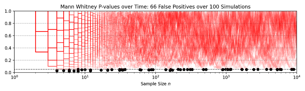
Have you ever encountered a bug while streaming Netflix? Did your title stop unexpectedly, or not start at all? In the first installment of this blog series on sequential testing, we described our canary testing methodology for continuous metrics such as play-delay. One of our readers commented

What if the new release is not related to a new play/streaming feature? For example, what if the new release includes modified login functionality? Will you still monitor the “play-delay” metric?

Netflix monitors a large suite of metrics, many of which can be classified as counts. These include metrics such as the number of logins, errors, successful play starts, and even the number of customer call center contacts. In this second installment, we describe our sequential methodology for testing count metrics, outlined in the NeurIPS paper Anytime Valid Inference for Multinomial Count Data.

Spot the Difference

Suppose we are about to deploy new code that changes the login behavior. To de-risk the software rollout we A/B test the new code, known also as a canary test. Whenever an event such as a login occurs, a log flows through our real-time backend and the corresponding timestamp is recorded. Figure 1 illustrates the sequences of timestamps generated by devices assigned to the new (treatment) and existing (control) software versions. A question that naturally concerns us is whether there are fewer login events in the treatment. Can you tell?

Figure 1: Timestamps of events occurring in control and treatment

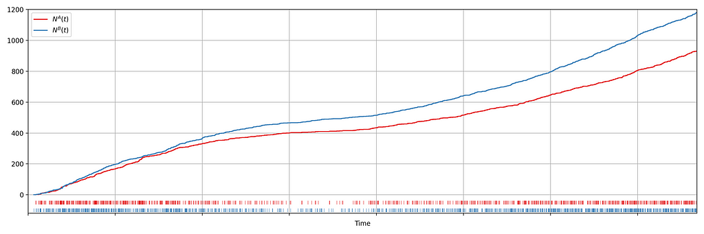
It is not immediately obvious by simple inspection of the point processes in Figure 1. The difference becomes immediately obvious when we visualize the observed counting processes, shown in Figure 2.

Figure 2: Visualizing the counting processes — the number of events observed by time t

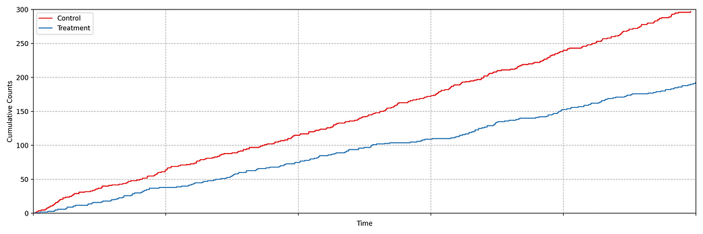
The counting processes are functions that increment by 1 whenever a new event arrives. Clearly, there are fewer events occurring in the treatment than in the control. If these were login events, this would suggest that the new code contains a bug that prevents some users from being able to log in successfully.

This is a common situation when dealing with event timestamps. To give another example, if events corresponded to errors or crashes, we would like to know if these are accruing faster in the treatment than in the control. Moreover, we want to answer that question as quickly as possible to prevent any further disruption to the service. This necessitates sequential testing techniques which were introduced in part 1.

Time-Inhomogeneous Poisson Process

Our data for each treatment group is a realization of a one-dimensional point process, that is, a sequence of timestamps. As the rate at which the events arrive is time-varying (in both treatment and control), we model the point process as a time-inhomogeneous Poisson point process. This point process is defined by an intensity function λ: ℝ → [0, ∞). The number of events in the interval [0,t), denoted N(t), has the following Poisson distribution

N(t) ~ Poisson(Λ(t)), where Λ(t) = ∫₀ᵗ λ(s) ds.

We seek to test the null hypothesis H₀: λᴬ(t) = λᴮ(t) for all t i.e. the intensity functions for control (A) and treatment (B) are the same. This can be done semiparametrically without making any assumptions about the intensity functions λᴬ and λᴮ. Moreover, the novelty of the research is that this can be done sequentially, as described in section 4 of our paper. Conveniently, the only data required to test this hypothesis at time t is Nᴬ(t) and Nᴮ(t), the total number of events observed so far in control and treatment. In other words, all you need to test the null hypothesis is two integers, which can easily be updated as new events arrive. Here is an example from a simulated A/A test, in which we know by design that the intensity function is the same for the control (A) and the treatment (B), albeit nonstationary.

Figure 3: (Left) An A/A simulation of two inhomogeneous Poisson point processes. (Right) Confidence sequence on the log-difference of intensity functions, and sequential p-value.

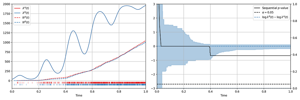
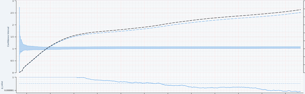
Figure 3 provides an illustration of an A/A setting. The left figure presents the raw data and the intensity functions, and the right figure presents the sequential statistical analysis. The blue and red rug plots indicate the observed arrival timestamps of events from the treatment and control streams respectively. The dashed lines are the observed counting processes. As this data is simulated under the null, the intensity functions are identical and overlay each other. The left axis of the right figure visualizes the evolution of the confidence sequence on the log-difference of intensity functions. The right axis of the right figure visualizes the evolution of the sequential p-value. We can make the two following observations

  • Under the null, the difference of log intensities is zero, which is correctly covered by the 0.95 confidence sequence at all times.
  • The sequential p-value is greater than 0.05 at all times

Now let’s consider an illustration of an A/B setting. Figure 4 shows observed arrival times for treatment and control when the intensity functions differ. As this is a simulation, the true difference between log intensities is known.

Figure 4: (Left) An A/B simulation of two inhomogeneous Poisson point processes. (Right) Confidence sequence on the difference of log of intensity functions, and sequential p-value.

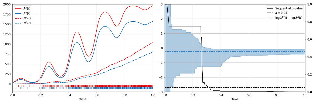
We can make the following observations

  • The 0.95 confidence sequence covers the true log-difference at all times
  • The sequential p-value falls below 0.05 at the same time the 0.95 confidence sequence excludes the null value of zero

Now we present a number of case studies where this methodology has rapidly detected serious problems in a number of count metrics

Case Study 1: Drop in Successful Title Starts

Figure 2 actually presents counts of title start events from a real canary test. Whenever a title starts successfully, an event is sent from the device to Netflix. We have a stream of title start events from treatment devices and a stream of title start events from control devices. Whenever fewer title starts are observed among treatment devices, there is usually a bug in the new client preventing playback.

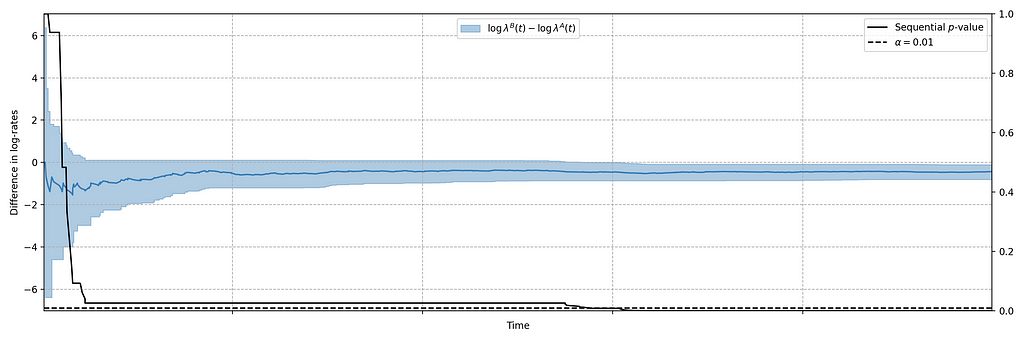
In this case, the canary test detected a bug that was later determined to have prevented approximately 60% of treatment devices from being able to start their streams. The confidence sequence is shown in Figure 5, in addition to the (sequential) p-value. While the exact units of time have been omitted, this bug was detected at the sub-second level.

Figure 5: 0.99 Confidence sequence on the difference of log-intensities with sequential p-value.

Case Study 2: Increase in Abnormal Shutdowns

In addition to title start events, we also monitor whenever the Netflix client shuts down unexpectedly. As before, we have two streams of abnormal shutdown events, one from treatment devices, and one from control devices. The following screenshots are taken directly from our Lumen dashboards.

Figure 6: Counts of Abnormal Shutdowns over time, cumulative and non-cumulative. Treatment (Black) and Control (Blue)

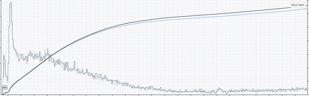
Figure 6 illustrates two important points. There is clearly nonstationarity in the arrival of abnormal shutdown events. It is also not easy to visibly see any difference between treatment and control from the non-cumulative view. The difference is, however, much easier to see from the cumulative view by observing the counting process. There is a small but visible increase in the number of abnormal shutdowns in the treatment. Figure 7 shows how our sequential statistical methodology is even able to identify such small differences.

Figure 7: Abnormal Shutdowns. (Top Panel) Confidence sequences on λᴮ(t)/λᴬ(t) (shaded blue) with observed counting processes for treatment (black dashed) and control (blue dashed). (Bottom Panel) sequential p-values.

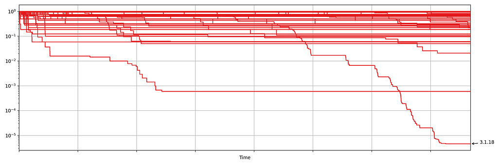
Case Study 3: Increase in Errors

Netflix also monitors the number of errors produced by treatment and control. This is a high cardinality metric as every error is annotated with a code indicating the type of error. Monitoring errors segmented by code helps developers diagnose issues quickly. Figure 8 shows the sequential p-values, on the log scale, for a set of error codes that Netflix monitors during client rollouts. In this example, we have detected a higher volume of 3.1.18 errors being produced by treatment devices. Devices experiencing this error are presented with the following message:

“We’re having trouble playing this title right now”

Figure 8: Sequential p-values for start play errors by error code
Figure 9: Observed error-3.1.18 timestamps and counting processes for treatment (blue) and control (red)

Knowing which errors increased can streamline the process of identifying the bug for our developers. We immediately send developers alerts through Slack integrations, such as the following

Figure 10: Notifications via Slack Integrations

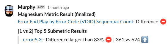
The next time you are watching Netflix and encounter an error, know that we’re on it!

Try it Out!

The statistical approach outlined in our paper is remarkably easy to implement in practice. All you need are two integers, the number of events observed so far in the treatment and control. The code is available in this short GitHub gist. Here are two usage examples:

> counts = [100, 101]
> assignment_probabilities = [0.5, 0.5]
> sequential_p_value(counts, assignment_probabilities)
1

> counts = [100, 201]
> assignment_probabilities = [0.5, 0.5]
> sequential_p_value(counts, assignment_probabilities)
5.06061172163498e-06

The code generalizes to more than just two treatment groups. For full details, including hyperparameter tuning, see section 4 of the paper.

Further Reading


Sequential Testing Keeps the World Streaming Netflix Part 2: Counting Processes was originally published in Netflix TechBlog on Medium, where people are continuing the conversation by highlighting and responding to this story.

Sequential A/B Testing Keeps the World Streaming Netflix Part 1: Continuous Data

Post Syndicated from Netflix Technology Blog original https://netflixtechblog.com/sequential-a-b-testing-keeps-the-world-streaming-netflix-part-1-continuous-data-cba6c7ed49df

Michael Lindon, Chris Sanden, Vache Shirikian, Yanjun Liu, Minal Mishra, Martin Tingley

Using sequential anytime-valid hypothesis testing procedures to safely release software

1. Spot the Difference

Can you spot any difference between the two data streams below? Each observation is the time interval between a Netflix member hitting the play button and playback commencing, i.e., play-delay. These observations are from a particular type of A/B test that Netflix runs called a software canary or regression-driven experiment. More on that below — for now, what’s important is that we want to quickly and confidently identify any difference in the distribution of play-delay — or conclude that, within some tolerance, there is no difference.

In this blog post, we will develop a statistical procedure to do just that, and describe the impact of these developments at Netflix. The key idea is to switch from a “fixed time horizon” to an “any-time valid” framing of the problem.

Sequentially comparing two streams of measurements from treatment and control
Figure 1. An example data stream for an A/B test where each observation represents play-delay for the control (left) and treatment (right). Can you spot any differences in the statistical distributions between the two data streams?

2. Safe software deployment, canary testing, and play-delay

Software engineering readers of this blog are likely familiar with unit, integration and load testing, as well as other testing practices that aim to prevent bugs from reaching production systems. Netflix also performs canary tests — software A/B tests between current and newer software versions. To learn more, see our previous blog post on Safe Updates of Client Applications.

The purpose of a canary test is twofold: to act as a quality-control gate that catches bugs prior to full release, and to measure performance of the new software in the wild. This is carried out by performing a randomized controlled experiment on a small subset of users, where the treatment group receives the new software update and the control group continues to run the existing software. If any bugs or performance regressions are observed in the treatment group, then the full-scale release can be prevented, limiting the “impact radius” among the user base.

One of the metrics Netflix monitors in canary tests is how long it takes for the video stream to start when a title is requested by a user. Monitoring this “play-delay” metric throughout releases ensures that the streaming performance of Netflix only ever improves as we release newer versions of the Netflix client. In Figure 1, the left side shows a real-time stream of play-delay measurements from users running the existing version of the Netflix client, while the right side shows play-delay measurements from users running the updated version. We ask ourselves: Are users of the updated client experiencing longer play-delays?

We consider any increase in play-delay to be a serious performance regression and would prevent the release if we detect an increase. Critically, testing for differences in means or medians is not sufficient and does not provide a complete picture. For example, one situation we might face is that the median or mean play-delay is the same in treatment and control, but the treatment group experiences an increase in the upper quantiles of play-delay. This corresponds to the Netflix experience being degraded for those who already experience high play delays — likely our members on slow or unstable internet connections. Such changes should not be ignored by our testing procedure.

For a complete picture, we need to be able to reliably and quickly detect an upward shift in any part of the play-delay distribution. That is, we must do inference on and test for any differences between the distributions of play-delay in treatment and control.

To summarize, here are the design requirements of our canary testing system:

  1. Identify bugs and performance regressions, as measured by play-delay, as quickly as possible. Rationale: To minimize member harm, if there is any problem with the streaming quality experienced by users in the treatment group we need to abort the canary and roll back the software change as quickly as possible.
  2. Strictly control false positive (false alarm) probabilities. Rationale: This system is part of a semi-automated process for all client deployments. A false positive test unnecessarily interrupts the software release process, reducing the velocity of software delivery and sending developers looking for bugs that do not exist.
  3. This system should be able to detect any change in the distribution. Rationale: We care not only about changes in the mean or median, but also about changes in tail behaviour and other quantiles.

We now build out a sequential testing procedure that meets these design requirements.

3. Sequential Testing: The Basics

Standard statistical tests are fixed-n or fixed-time horizon: the analyst waits until some pre-set amount of data is collected, and then performs the analysis a single time. The classic t-test, the Kolmogorov-Smirnov test, and the Mann-Whitney test are all examples of fixed-n tests. A limitation of fixed-n tests is that they can only be performed once — yet in situations like the above, we want to be testing frequently to detect differences as soon as possible. If you apply a fixed-n test more than once, then you forfeit the Type-I error or false positive guarantee.

Here’s a quick illustration of how fixed-n tests fail under repeated analysis. In the following figure, each red line traces out the p-value when the Mann-Whitney test is repeatedly applied to a data set as 10,000 observations accrue in both treatment and control. Each red line shows an independent simulation, and in each case, there is no difference between treatment and control: these are simulated A/A tests.

The black dots mark where the p-value falls below the standard 0.05 rejection threshold. An alarming 70% of simulations declare a significant difference at some point in time, even though, by construction, there is no difference: the actual false positive rate is much higher than the nominal 0.05. Exactly the same behaviour would be observed for the Kolmogorov-Smirnov test.

increased false positives when peeking at mann-whitney test
Figure 2. 100 Sample paths of the p-value process simulated under the null hypothesis shown in red. The dotted black line indicates the nominal alpha=0.05 level. Black dots indicate where the p-value process dips below the alpha=0.05 threshold, indicating a false rejection of the null hypothesis. A total of 66 out of 100 A/A simulations falsely rejected the null hypothesis.

This is a manifestation of “peeking”, and much has been written about the downside risks of this practice (see, for example, Johari et al. 2017). If we restrict ourselves to correctly applied fixed-n statistical tests, where we analyze the data exactly once, we face a difficult tradeoff:

  • Perform the test early on, after a small amount of data has been collected. In this case, we will only be powered to detect larger regressions. Smaller performance regressions will not be detected, and we run the risk of steadily eroding the member experience as small regressions accrue.
  • Perform the test later, after a large amount of data has been collected. In this case, we are powered to detect small regressions — but in the case of large regressions, we expose members to a bad experience for an unnecessarily long period of time.

Sequential, or “any-time valid”, statistical tests overcome these limitations. They permit for peeking –in fact, they can be applied after every new data point arrives– while providing false positive, or Type-I error, guarantees that hold throughout time. As a result, we can continuously monitor data streams like in the image above, using confidence sequences or sequential p-values, and rapidly detect large regressions while eventually detecting small regressions.

Despite relatively recent adoption in the context of digital experimentation, these methods have a long academic history, with initial ideas dating back to Abraham Wald’s Sequential Tests of Statistical Hypotheses from 1945. Research in this area remains active, and Netflix has made a number of contributions in the last few years (see the references in these papers for a more complete literature review):

In this and following blogs, we will describe both the methods we’ve developed and their applications at Netflix. The remainder of this post discusses the first paper above, which was published at KDD ’22 (and available on ArXiV). We will keep it high level — readers interested in the technical details can consult the paper.

4. A sequential testing solution

Differences in Distributions

At any point in time, we can estimate the empirical quantile functions for both treatment and control, based on the data observed so far.

empirical quantile functions for treatment and control data
Figure 3: Empirical quantile function for control (left) and treatment (right) at a snapshot in time after starting the canary experiment. This is from actual Netflix data, so we’ve suppressed numerical values on the y-axis.

These two plots look pretty close, but we can do better than an eyeball comparison — and we want the computer to be able to continuously evaluate if there is any significant difference between the distributions. Per the design requirements, we also wish to detect large effects early, while preserving the ability to detect small effects eventually — and we want to maintain the false positive probability at a nominal level while permitting continuous analysis (aka peeking).

That is, we need a sequential test on the difference in distributions.

Obtaining “fixed-horizon” confidence bands for the quantile function can be achieved using the DKWM inequality. To obtain time-uniform confidence bands, however, we use the anytime-valid confidence sequences from Howard and Ramdas (2022) [arxiv version]. As the coverage guarantee from these confidence bands holds uniformly across time, we can watch them become tighter without being concerned about peeking. As more data points stream in, these sequential confidence bands continue to shrink in width, which means any difference in the distribution functions — if it exists — will eventually become apparent.

Anytime-valid confidence bands on treatment and control quantile functions
Figure 4: 97.5% Time-Uniform Confidence bands on the quantile function for control (left) and treatment (right)

Note each frame corresponds to a point in time after the experiment began, not sample size. In fact, there is no requirement that each treatment group has the same sample size.

Differences are easier to see by visualizing the difference between the treatment and control quantile functions.

Confidence sequences on quantile differences and sequential p-value
Figure 5: 95% Time-Uniform confidence band on the quantile difference function Q_b(p) — Q_a(p) (left). The sequential p-value (right).

As the sequential confidence band on the treatment effect quantile function is anytime-valid, the inference procedure becomes rather intuitive. We can continue to watch these confidence bands tighten, and if at any point the band no longer covers zero at any quantile, we can conclude that the distributions are different and stop the test. In addition to the sequential confidence bands, we can also construct a sequential p-value for testing that the distributions differ. Note from the animation that the moment the 95% confidence band over quantile treatment effects excludes zero is the same moment that the sequential p-value falls below 0.05: as with fixed-n tests, there is consistency between confidence intervals and p-values.

There are many multiple testing concerns in this application. Our solution controls Type-I error across all quantiles, all treatment groups, and all joint sample sizes simultaneously (see our paper, or Howard and Ramdas for details). Results hold for all quantiles, and for all times.

5. Impact at Netflix

Releasing new software always carries risk, and we always want to reduce the risk of service interruptions or degradation to the member experience. Our canary testing approach is another layer of protection for preventing bugs and performance regressions from slipping into production. It’s fully automated and has become an integral part of the software delivery process at Netflix. Developers can push to production with peace of mind, knowing that bugs and performance regressions will be rapidly caught. The additional confidence empowers developers to push to production more frequently, reducing the time to market for upgrades to the Netflix client and increasing our rate of software delivery.

So far this system has successfully prevented a number of serious bugs from reaching our end users. We detail one example.

Case study: Safe Rollout of Netflix Client Application

Figures 3–5 are taken from a canary test in which the behaviour of the client application was modified application (actual numerical values of play-delay have been suppressed). As we can see, the canary test revealed that the new version of the client increases a number of quantiles of play-delay, with the median and 75% percentile of play experiencing relative increases of at least 0.5% and 1% respectively. The timeseries of the sequential p-value shows that, in this case, we were able to reject the null of no change in distribution at the 0.05 level after about 60 seconds. This provides rapid feedback in the software delivery process, allowing developers to test the performance of new software and quickly iterate.

6. What’s next?

If you are curious about the technical details of the sequential tests for quantiles developed here, you can learn all about the math in our KDD paper (also available on arxiv).

You might also be wondering what happens if the data are not continuous measurements. Errors and exceptions are critical metrics to log when deploying software, as are many other metrics which are best defined in terms of counts. Stay tuned — our next post will develop sequential testing procedures for count data.


Sequential A/B Testing Keeps the World Streaming Netflix
Part 1: Continuous Data
was originally published in Netflix TechBlog on Medium, where people are continuing the conversation by highlighting and responding to this story.

Growth Engineering at Netflix- Creating a Scalable Offers Platform

Post Syndicated from Netflix Technology Blog original https://netflixtechblog.com/growth-engineering-at-netflix-creating-a-scalable-offers-platform-69330136dd87

by Eric Eiswerth

Background

Netflix has been offering streaming video-on-demand (SVOD) for over 10 years. Throughout that time we’ve primarily relied on 3 plans (Basic, Standard, & Premium), combined with the 30-day free trial to drive global customer acquisition. The world has changed a lot in this time. Competition for people’s leisure time has increased, the device ecosystem has grown phenomenally, and consumers want to watch premium content whenever they want, wherever they are, and on whatever device they prefer. We need to be constantly adapting and innovating as a result of this change.

The Growth Engineering team is responsible for executing growth initiatives that help us anticipate and adapt to this change. In particular, it’s our job to design and build the systems and protocols that enable customers from all over the world to sign up for Netflix with the plan features and incentives that best suit their needs. For more background on Growth Engineering and the signup funnel, please have a look at our previous blog post that covers the basics. Alternatively, here’s a quick review of what the typical user journey for a signup looks like:

Signup Funnel Dynamics

There are 3 steps in a basic Netflix signup. We refer to these steps that comprise a user journey as a signup flow. Each step of the flow serves a distinct purpose.

  1. Introduction and account creation
    Highlight our value propositions and begin the account creation process.
  2. Plans & offers
    Highlight the various types of Netflix plans, along with any potential offers.
  3. Payment
    Highlight the various payment options we have so customers can choose what suits their needs best.

The primary focus for the remainder of this post will be step 2: plans & offers. In particular, we’ll define plans and offers, review the legacy architecture and some of its shortcomings, and dig into our new architecture and some of its advantages.

Plans & Offers

Definitions

Let’s define what a plan and an offer is at Netflix. A plan is essentially a set of features with a price.

An offer is an incentive that typically involves a monetary discount or superior product features for a limited amount of time. Broadly speaking, an offer consists of one or more incentives and a set of attributes.

When we merge these two concepts together and present them to the customer, we have the plan selection page (shown above). Here, you can see that we have 3 plans and a 30-day free trial offer, regardless of which plan you choose. Let’s take a deeper look at the architecture, protocols, and systems involved.

Legacy Architecture

As previously mentioned, Netflix has had a relatively static set of plans and offers since the inception of streaming. As a result of this simple product offering, the architecture was also quite straightforward. It consisted of a small set of XML files that were loaded at runtime and stored in local memory. This was a perfectly sufficient design for many years. However, there are some downsides as the company continues to grow and the product continues to evolve. To name a few:

  • Updating XML files is error-prone and manual in nature.
  • A full deployment of the service is required whenever the XML files are updated.
  • Updating the XML files requires engaging domain experts from the backend engineering team that owns these files. This pulls them away from other business-critical work and can be a distraction.
  • A flat domain object structure that resulted in client-side logic in order to extract relevant plan and offer information in order to render the UI. For example, consider the data structure for a 30 day free trial on the Basic plan.
{
"offerId": 123,
"planId": 111,
"price": "$8.99",
"hasSD": true,
"hasHD": false,
"hasFreeTrial": true,
etc…
}
  • As the company matures and our product offering adapts to our global audience, all of the above issues are exacerbated further.

Below is a visual representation of the various systems involved in retrieving plan and offer data. Moving forward, we’ll refer to the combination of plan and offer data simply as SKU (Stock Keeping Unit) data.

New Architecture

If you recall from our previous blog post, Growth Engineering owns the business logic and protocols that allow our UI partners to build lightweight and flexible applications for almost any platform. This implies that the presentation layer should be void of any business logic and should simply be responsible for rendering data that is passed to it. In order to accomplish this we have designed a microservice architecture that emphasizes the Separation of Concerns design principle. Consider the updated system interaction diagram below:

There are 2 noteworthy changes that are worth discussing further. First, notice the presence of a dedicated SKU Eligibility Service. This service contains specialized business logic that used to be part of the Orchestration Service. By migrating this logic to a new microservice we simplify the Orchestration Service, clarify ownership over the domain, and unlock new use cases since it is now possible for other services not shown in this diagram to also consume eligible SKU data.

Second, notice that the SKU Service has been extended to a platform, which now leverages a rules engine and SKU catalog DB. This platform unlocks tremendous business value since product-oriented teams are now free to use the platform to experiment with different product offerings for our global audience, with little to no code changes required. This means that engineers can spend less time doing tedious work and more time designing creative solutions to better prepare us for future needs. Let’s take a deeper look at the role of each service involved in retrieving SKU data, starting from the visitor’s device and working our way down the stack.

Step 1 — Device sends a request for the plan selection page
As discussed in our previous Growth Engineering blog post, we use a custom JSON protocol between our client UIs and our middle-tier Orchestration Service. An example of what this protocol might look like for a browser request to retrieve the plan selection page shown above might look as follows:

GET /plans
{
“flow”: “browser”,
“mode”: “planSelection”
}

As you can see, there are 2 critical pieces of information in this request:

  • Flow — The flow is a way to identify the platform. This allows the Orchestration Service to route the request to the appropriate platform-specific request handling logic.
  • Mode — This is essentially the name of the page being requested.

Given the flow and mode, the Orchestration Service can then process the request.

Step 2 — Request is routed to the Orchestration Service for processing
The Orchestration Service is responsible for validating upstream requests, orchestrating calls to downstream services, and composing JSON responses during a signup flow. For this particular request the Orchestration Service needs to retrieve the SKU data from the SKU Eligibility Service and build the JSON response that can be consumed by the UI layer.

The JSON response for this request might look something like below. Notice the difference in data structures from the legacy implementation. This new contextual representation facilitates greater reuse, as well as potentially supporting offers other than a 30 day free trial:

{
“flow”: “browser”,
“mode”: “planSelection”,
“fields”: {
“skus”: [
{
“id”: 123,
“incentives”: [“FREE_TRIAL”],
“plan”: {
“name”: “Basic”,
“quality”: “SD”,
“price” : “$8.99”,
...
}
...
},
{
“id”: 456,
“incentives”: [“FREE_TRIAL”],
“plan”: {
“name”: “Standard”,
“quality”: “HD”,
“price” : “$13.99”,
...
}
...
},
{
“id”: 789,
“incentives”: [“FREE_TRIAL”],
“plan”: {
“name”: “Premium”,
“quality”: “UHD”,
“price” : “$17.99”,
...
}
...
}
],
“selectedSku”: {
“type”: “Numeric”,
“value”: 789
}
"nextAction": {
"type": "Action"
"withFields": [
"selectedSku"
]
}
}
}

As you can see, the response contains a list of SKUs, the selected SKU, and an action. The action corresponds to the button on the page and the withFields specify which fields the server expects to have sent back when the button is clicked.

Step 3 & 4 — Determine eligibility and retrieve eligible SKUs from SKU Eligibility Service
Netflix is a global company and we often have different SKUs in different regions. This means we need to distinguish between availability of SKUs and eligibility for SKUs. You can think of eligibility as something that is applied at the user level, while availability is at the country level. The SKU Platform contains the global set of SKUs and as a result, is said to control the availability of SKUs. Eligibility for SKUs is determined by the SKU Eligibility Service. This distinction creates clear ownership boundaries and enables the Growth Engineering team to focus on surfacing the correct SKUs for our visitors.

This centralization of eligibility logic in the SKU Eligibility Service also enables innovation in different parts of the product that have traditionally been ignored. Different services can now interface directly with the SKU Eligibility Service in order to retrieve SKU data.

Step 5 — Retrieve eligible SKUs from SKU Platform
The SKU Platform consists of a rules engine, a database, and application logic. The database contains the plans, prices and offers. The rules engine provides a means to extract available plans and offers when certain conditions within a rule match. Let’s consider a simple example where we attempt to retrieve offers in the US.

Keeping the Separation of Concerns in mind, notice that the SKU Platform has only one core responsibility. It is responsible for managing all Netflix SKUs. It provides access to these SKUs via a simple API that takes customer context and attempts to match it against the set of SKU rules. SKU eligibility is computed upstream and is treated just as any other condition would be in the SKU ruleset. By not coupling the concepts of eligibility and availability into a single service, we enable increased developer productivity since each team is able to focus on their core competencies and any change in eligibility does not affect the SKU Platform. One of the core tenets of a platform is the ability to support self-service. This negates the need to engage the backend domain experts for every desired change. The SKU Platform supports this via lightweight configuration changes to rules that do not require a full deployment. The next step is to invest further into self-service and support rule changes via a SKU UI. Stay tuned for more details on this, as well as more details on the internals of the new SKU Platform in one of our upcoming blog posts.

Conclusion

This work was a large cross-functional effort. We rebuilt our offers and plans from the ground up. It resulted in systems changes, as well as interaction changes between teams. Where there was once ambiguity, we now have clearly defined ownership over SKU availability and eligibility. We are now capable of introducing new plans and offers in various markets around the globe in order to meet our customer’s needs, with minimal engineering effort.

Let’s review some of the advantages the new architecture has over the legacy implementation. To name a few:

  • Domain objects that have a more reusable and extensible “shape”. This shape facilitates code reuse at the UI layer as well as the service layers.
  • A SKU Platform that enables product innovation with minimal engineering involvement. This means engineers can focus on more challenging and creative solutions for other problems. It also means fewer engineering teams are required to support initiatives in this space.
  • Configuration instead of code for updating SKU data, which improves innovation velocity.
  • Lower latency as a result of fewer service calls, which means fewer errors for our visitors.

The world is constantly changing. Device capabilities continue to improve. How, when, and where people want to be entertained continues to evolve. With these types of continued investments in infrastructure, the Growth Engineering team is able to build a solid foundation for future innovations that will allow us to continue to deliver the best possible experience for our members.

Join Growth Engineering and help us build the next generation of services that will allow the next 200 million subscribers to experience the joy of Netflix.


Growth Engineering at Netflix- Creating a Scalable Offers Platform was originally published in Netflix TechBlog on Medium, where people are continuing the conversation by highlighting and responding to this story.

Growth Engineering at Netflix — Automated Imagery Generation

Post Syndicated from Netflix Technology Blog original https://netflixtechblog.com/growth-engineering-at-netflix-automated-imagery-generation-5a105fd51569

Growth Engineering at Netflix — Automated Imagery Generation

by Eric Eiswerth

Background

There’s a good chance you’ve probably visited the Netflix homepage. In the Growth Engineering team, we refer to this as the top of the signup funnel. For more background on the signup funnel and Growth Engineering’s role in the signup funnel, please read our initial post on the topic: Growth Engineering at Netflix — Accelerating Innovation. The primary focus of this post will be the top of the signup funnel. In particular, the Netflix homepage:

As discussed in our previous post, Growth Engineering owns the business logic and protocols that allow our UI partners to build lightweight and flexible applications for almost any platform. In some cases, like the homepage, this even involves providing appropriate imagery (e.g., the background image shown above). In this post, we’ll take a deep dive into the journey of content-based imagery on the Netflix homepage.

Motivation

At Netflix we do one thing — entertainment — and we aim to do it really well. We live and breathe TV shows and films, and we want everyone to be able to enjoy them too. That’s why we aspire to have best in class stories, across genres and believe people should have access to new voices, cultures and perspectives. The member-focused teams at Netflix are responsible for making sure the member experience is relevant and personalized, ensuring that this content is shown to the right people at the right time. But what about non-members; those who are simply interested in signing up for Netflix, how should we highlight our content and convey our value propositions to them?

The Solution

The main mechanism for highlighting our content in the signup flow is through content-based imagery. Before designing a solution it’s important to understand the main product requirements for such a feature:

  • The content needs to be new, relevant, and regional (not all countries have the same catalogue).
  • The artwork needs to appeal to a broader audience. The non-member homepage serves a very broad audience and is not personalized to the extent of the member experience.
  • The imagery needs to be localized.
  • We need to be able to easily determine what imagery is present for a given platform, region, and language.
  • The homepage needs to load in a reasonable amount of time, even in poor network conditions.

Unpacking Product Requirements

Given the scale we require and the product requirements listed above, there are a number of technical requirements:

  • A list of titles for the asset, in some order.
  • Ensure the titles are appropriate for a broad audience, which means all titles need to be tagged with metadata.
  • Localized images for each of the titles.
  • Different assets for different device types and screen sizes.
  • Server-generated assets, since client-side generation would require the retrieval of many individual images, which would increase latency and time-to-render.
  • To reduce latency, assets should be generated in an offline fashion and not in real time.
  • The assets need to be compressed, without reducing quality significantly.
  • The assets will need to be stored somewhere and we’ll need to generate URLs for each of them.
  • We’ll need to figure out how to provide the correct asset URL for a given request.
  • We’ll need to build a search index so that the assets can be searchable.

Given this set of requirements, we can effectively break this work down into 3 functional buckets:

The Design

For our design, we decided to build 3 separate microservices, mapping to the aforementioned functional buckets. Let’s take a look at each of these services in turn.

Asset Generation

The Asset Generation Service is responsible for generating groups of assets. We call these groups of assets, asset groups. Each request will generate a single asset group that will contain one or more assets. To support the demands of our stakeholders we designed a Domain Specific Language (DSL) that we call an asset generation recipe. An asset generation request contains a recipe. Below is an example of a simple recipe:

{
"titleIds": [12345, 23456, 34567, …],
"countries": [“US”],
"type": “perspective”, // this is the design of the asset
"rows": 10, // the number of rows and columns can control density
"cols": 15,
"padding": 10, // padding between individual images
"columnOffsets": [0, 0, 0, 0…], // the y-offset for each column
"rowOffsets": [0, -100, 0, -100, …], // the x-offset for each row
"size": [1920, 1080] // size in pixels
}

This recipe can then be issued via an HTTP POST request to the Asset Generation Service. The recipe can then be translated into ImageMagick commands that can do the heavy lifting. At a high level, the following diagram captures the necessary steps required to build an asset.

Generating a single localized asset is a big achievement, but we still need to store the asset somewhere and have the ability to search for it. This requires an asset storage solution.

Asset Storage

We refer to asset storage and management simply as asset management. We felt it would be beneficial to create a separate microservice for asset management for 2 reasons. First, asset generation is CPU intensive and bursty. We can leverage high performance VMs in AWS to generate the assets. We can scale up when generation is occurring and scale down when there is no batch in the queue. However, it would be cost-inefficient to leverage this same hardware for lightweight and more consistent traffic patterns that an asset management service requires.

Let’s take a look at the internals of the Asset Management Service.

At this point we’ve laid out all the details in order to generate a content-based asset and have it stored as part of an asset group, which is persisted and indexed. The next thing to consider is, how do we retrieve an asset in real time and surface it on the Netflix homepage?

If you recall in our previous blog post, Growth Engineering owns a service called the Orchestration Service. It is a mid-tier service that emits a custom JSON data structure that contains fields that are consumed by the UI. The UI can then use these fields to control the presentation in the UI layer. There are two approaches for adding fields to the Orchestration Service’s response. First, the fields can be coded by hand. Second, fields can be added via configuration via a service we call the Customization Service. Since assets will need to be periodically refreshed and we want this process to be entirely automated, it makes sense to pursue the configuration-based approach. To accomplish this, the Asset Management Service needs to translate an asset group into a rule definition for the Customization Service.

Customization Service

Let’s review the Orchestration Service and introduce the Customization Service. The Orchestration Service emits fields in response to upstream requests. For the homepage, there are typically only a small number of fields provided by the Orchestration Service. The following fields are supplied by application code. For example:

{
“fields”: {
“email” : {
“type”: “StringField”,
“value”: “”
},
“nextAction”: {
“type”: “Action”,
“withFields” [“email”]
}
}
}

The Orchestration Service also supports fields supplied by configuration. We call these adaptive fields. Adaptive fields are provided by the Customization Service. The Customization Service is a rules engine that emits the adaptive fields. For example, a rule to provide the background image for the homepage in the en-US locale would look as follows:

{
“country”: “US”,
“language”: “en”,
“platform”: “browser”,
“resolution”: “high”
}

The corresponding payload for such a rule might look as follows:

{
“backgroundImage”: “https://cdn.netflix.com/bgimageurl.jpg”
}

Bringing this all together, the response from the Orchestration Service would now look as follows:

{
“fields”: {
“email” : {
“type”: “StringField”,
“value”: “”
},
“nextAction”: {
“type”: “Action”,
“withFields” [“email”]
}
},
“adaptiveFields”: {
“backgroundImage”: “https://cdn.netflix.com/bgimageurl.jpg”
}
}

At this point, we are now able to generate an asset, persist it, search it, and generate customization rules for it. The generated rules then enable us to return a particular asset for a particular request. Let’s put it all together and review the system interaction diagram.

We now have all the pieces in place to automatically generate artwork and have that artwork appear on the Netflix homepage for a given request. At least one open question remains, how can we scale asset generation?

Scaling Asset Generation

Arguably, there are a number of approaches that could be used to scale asset generation. We decided to opt for an all-or-nothing approach. Meaning, all assets for a given recipe need to be generated as a single asset group. This enables smooth rollback in case of any errors. Additionally, asset generation is CPU intensive and each recipe can produce 1000s of assets as a result of the number of platform, region, and language permutations. Even with high performance VMs, generating 1000s of assets can take a long time. As a result, we needed to find a way to distribute asset generation across multiple VMs. Here’s what the final architecture looked like.

Briefly, let’s review the steps:

  1. The batch process is initiated by a cron job. The job executes a script that contains an asset generation recipe.
  2. The Asset Generation Service receives the request and creates asset generation tasks that can be distributed across any number of Asset Generation Worker nodes. One of the nodes is elected as the leader via Zookeeper. Its job is to coordinate asset generation across the other workers and ensure all assets get generated.
  3. Once the primary worker node has all the assets, it creates an asset group in the Asset Management Service. The Asset Management Service persists, indexes, and uploads the assets to the CDN.
  4. Finally, the Asset Management Service creates rules from the asset group and pushes the rules to the Customization Service. Once the data is published in the Customization Service, the Orchestration Service can supply the correct URLs in its JSON response by invoking the Customization Service with a request context that matches a given set of rules.

Conclusion

Automated asset generation has proven to be an extremely valuable investment. It is low-maintenance, high-leverage, and has allowed us to experiment with a variety of different types of assets on different platforms and on different parts of the product. This project was technically challenging and highly rewarding, both to the engineers involved in the project, and to the business. The Netflix homepage has come a long way over the last several years.

We’re hiring! Join Growth Engineering and help us build the future of Netflix.


Growth Engineering at Netflix — Automated Imagery Generation was originally published in Netflix TechBlog on Medium, where people are continuing the conversation by highlighting and responding to this story.