Accessing private content online, whether it’s checking email or streaming your favorite show, almost always starts with a “login” step. Beneath this everyday task lies a widespread human mistake we still have not resolved: password reuse. Many users recycle passwords across multiple services, creating a ripple effect of risk when their credentials are leaked.
Based on Cloudflare’s observed traffic between September – November 2024, 41% of successful logins across websites protected by Cloudflare involve compromised passwords. In this post, we’ll explore the widespread impact of password reuse, focusing on how it affects popular Content Management Systems (CMS), the behavior of bots versus humans in login attempts, and how attackers exploit stolen credentials to take over accounts at scale.
Scope of the analysis
Our data analysis focuses on traffic from Internet properties on Cloudflare’s free plan, which includes leaked credentials detection as a built-in feature. Leaked credentials refer to usernames and passwords exposed in known data breaches or credential dumps — for this analysis, our focus is specifically on leaked passwords. With 30 million Internet properties, comprising some 20% of the web, behind Cloudflare, this analysis provides significant insights. The data primarily reflects trends observed after the detection system was launched during Birthday Week in September 2024.
Nearly 41% of logins are at risk
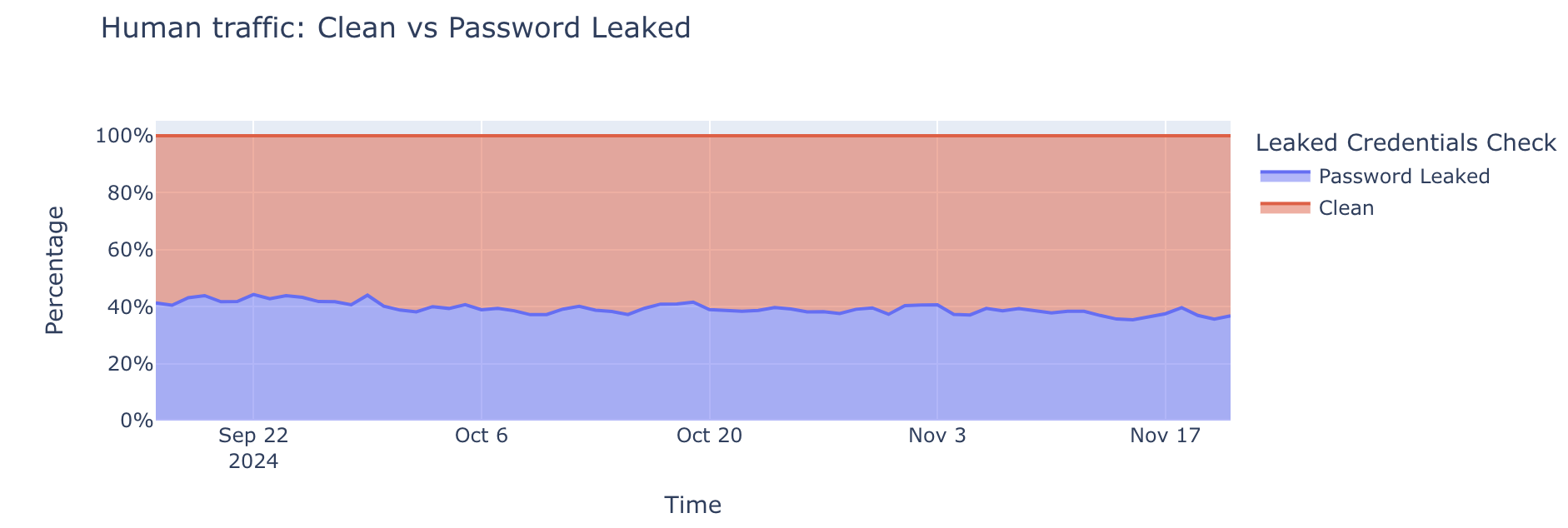
One of the biggest challenges in authentication is distinguishing between legitimate human users and malicious actors. To understand human behavior, we focus on successful login attempts (those returning a 200 OK status code), as this provides the clearest indication of user activity and real account risk. Our data reveals that approximately 41% of successful human authentication attempts involve leaked credentials.
Despite growing awareness about online security, a significant portion of users continue to reuse passwords across multiple accounts. And according to a recent study by Forbes, users will, on average, reuse their password across four different accounts. Even after major breaches, many individuals don’t change their compromised passwords, or still use variations of them across different services. For these users, it’s not a matter of “if” attackers will use their compromised passwords, it’s a matter of “when”.
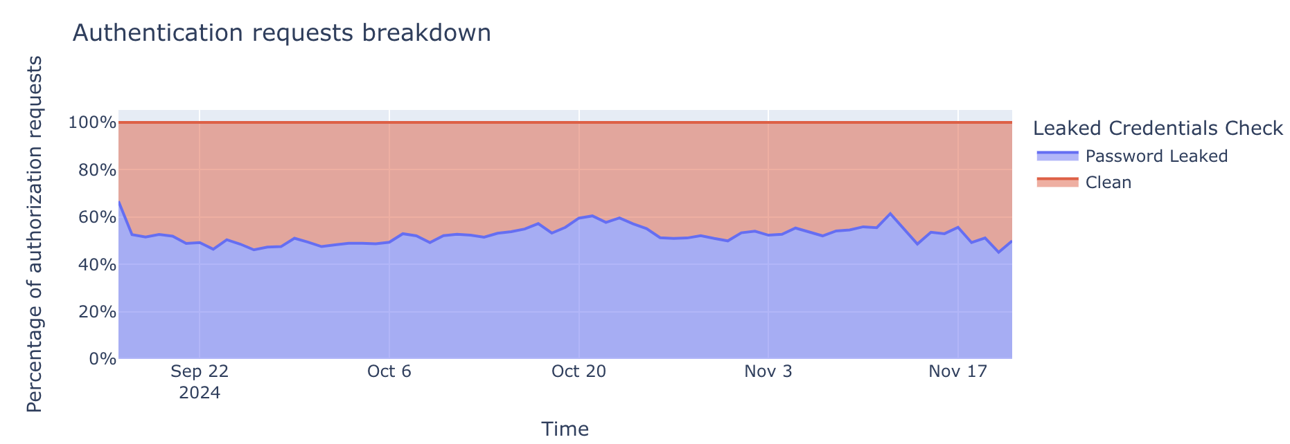
When we expand to include bot-driven traffic in this analysis, the problem of leaked credentials becomes even more noticeable. Our data reveals that 52% of all detected authentication requests contain leaked passwords found in our database of over 15 billion records, including the Have I Been Pwned (HIBP) leaked password dataset.
This percentage represents hundreds of millions of daily authentication requests, originating from both bots and humans. While not every attempt succeeds, the sheer volume of leaked credentials in real-world traffic illustrates how common password reuse is. Many of these leaked credentials still grant valid access, amplifying the risk of account takeovers.
Attackers heavily use leaked password datasets
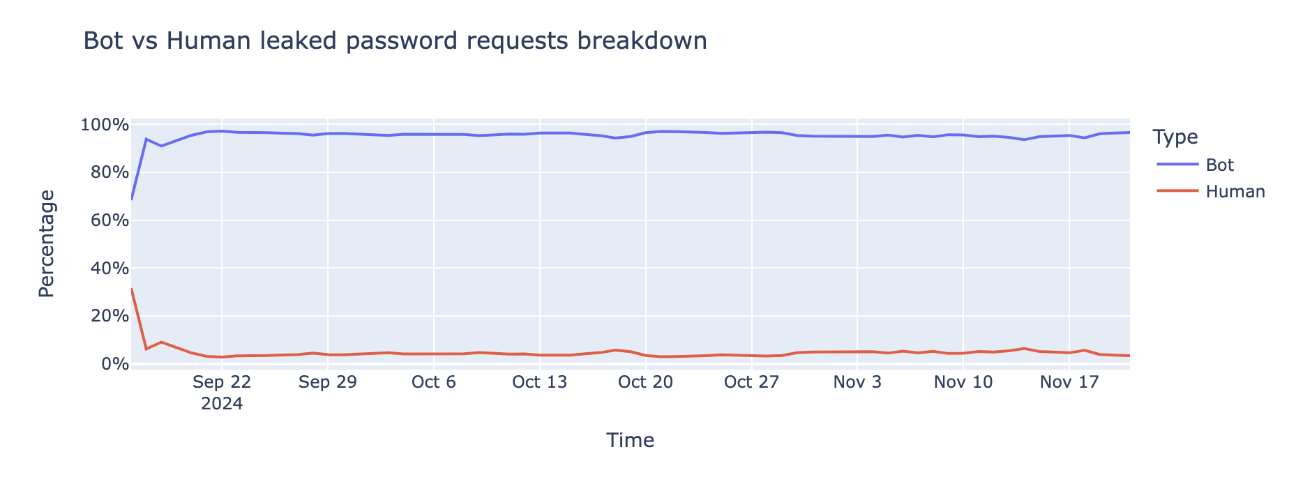
Bots are the driving force behind credential-stuffing attacks, the data indicates that95% of login attempts involving leaked passwords are coming from bots,indicating that they are part of credential stuffing attacks.
Equipped with credentials stolen from breaches, bots systematically target websites at scale, testing thousands of login combinations in seconds.
Data from the Cloudflare network exposes this trend, showing that bot-driven attacks remain alarmingly high over time. Popular platforms like WordPress, Joomla, and Drupal are frequent targets, due to their widespread use and exploitable vulnerabilities, as we will explore in the upcoming section.
Once bots successfully breach one account, attackers reuse the same credentials across other services to amplify their reach. They even sometimes try to evade detection by using sophisticated evasion tactics, such as spreading login attempts across different source IP addresses or mimicking human behavior, attempting to blend into legitimate traffic.
The result is a constant, automated threat vector that challenges traditional security measures and exploits the weakest link: password reuse.
Brute force attacks against WordPress
Content Management Systems (CMS) are used to build websites, and often rely on simple authentication and login plugins. This is convenient, but also makes them frequent targets of credential stuffing attacks due to their widespread adoption. WordPress is a very popular content management system with a well known user login page format. Because of this, websites built on WordPress often become common targets for attackers.
Across our network, WordPress accounts for a significant portion of authentication requests. This is unsurprising given its market share. However, what stands out is the alarming number of successful logins using leaked passwords, especially by bots.
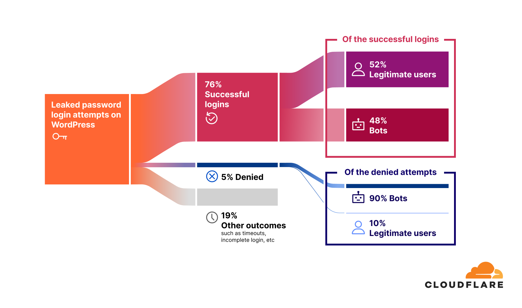
76% of leaked password login attempts for websites built on WordPress are successful.
Of these, 48% of successful logins are bot-driven.This is a shocking figure that indicates nearly half of all successful logins are executed by unauthorized systems designed to exploit stolen credentials. Successful unauthorized access is often the first step in account takeover (ATO) attacks.
The remaining 52% of successful logins originate from legitimate, non-bot users. This figure, higher than the average of 41% across all platforms, highlights how pervasive password reuse is among real users, putting their accounts at significant risk.
Only 5% of leaked password login attempts result in access being denied.
This is a low number compared to the successful bot-driven login attempts, and could be tied to a lack of security measures like rate-limiting or multi-factor authentication (MFA). If such measures were in place, we would expect the share of denied attempts to be higher. Notably, 90% of these denied requests are bot-driven, reinforcing the idea that while some security measures are blocking automated logins, many still slip through.
The overwhelming presence of bot traffic in this category points to ongoing automated attempts to brute-force access.
The remaining 19% of login attempts fall under other outcomes, such as timeouts, incomplete logins, or users who changed their passwords, so they neither count as direct “successes” nor do they register as “denials”.
Keeping user accounts safe with Cloudflare
If you’re a user, start with changing reused or weak passwords and use unique, strong ones for each website or application. Enable multi-factor authentication (MFA) on all of your accounts that support it, and start exploring passkeys as a more secure, phishing-resistant alternative to traditional passwords.
For website owners, activate leaked credentials detection to monitor and address these threats in real time and issue password reset flows on leaked credential matches.
Additionally, enable features like Rate Limiting and Bot Management tools to minimize the impact of automated attacks. Audit password reuse patterns, identify leaked credentials within your systems, and enforce robust password hygiene policies to strengthen overall security.
By adopting these measures, both individuals and organizations can stay ahead of attackers and build stronger defenses.
We are excited to share our work on how to learn good proxy metrics from historical experiments at KDD 2024. This work addresses a fundamental question for technology companies and academic researchers alike: how do we establish that a treatment that improves short-term (statistically sensitive) outcomes also improves long-term (statistically insensitive) outcomes? Or, faced with multiple short-term outcomes, how do we optimally trade them off for long-term benefit?
For example, in an A/B test, you may observe that a product change improves the click-through rate. However, the test does not provide enough signal to measure a change in long-term retention, leaving you in the dark as to whether this treatment makes users more satisfied with your service. The click-through rate is a proxy metric (S, for surrogate, in our paper) while retention is a downstream business outcome or north star metric (Y). We may even have several proxy metrics, such as other types of clicks or the length of engagement after click. Taken together, these form a vector of proxy metrics.
The goal of our work is to understand the true relationship between the proxy metric(s) and the north star metric — so that we can assess a proxy’s ability to stand in for the north star metric, learn how to combine multiple metrics into a single best one, and better explore and compare different proxies.
Several intuitive approaches to understanding this relationship have surprising pitfalls:
Looking only at user-level correlations between the proxy S and north star Y. Continuing the example from above, you may find that users with a higher click-through rate also tend to have a higher retention. But this does not mean that a product change that improves the click-through rate will also improve retention (in fact, promoting clickbait may have the opposite effect). This is because, as any introductory causal inference class will tell you, there are many confounders between S and Y — many of which you can never reliably observe and control for.
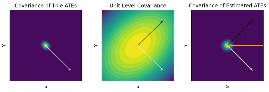
Looking naively at treatment effect correlations between S and Y. Suppose you are lucky enough to have many historical A/B tests. Further imagine the ordinary least squares (OLS) regression line through a scatter plot of Y on S in which each point represents the (S,Y)-treatment effect from a previous test. Even if you find that this line has a positive slope, you unfortunately cannot conclude that product changes that improve S will also improve Y. The reason for this is correlated measurement error — if S and Y are positively correlated in the population, then treatment arms that happen to have more users with high S will also have more users with high Y.
Between these naive approaches, we find that the second one is the easier trap to fall into. This is because the dangers of the first approach are well-known, whereas covariances between estimated treatment effects can appear misleadingly causal. In reality, these covariances can be severely biased compared to what we actually care about: covariances between true treatment effects. In the extreme — such as when the negative effects of clickbait are substantial but clickiness and retention are highly correlated at the user level — the true relationship between S and Y can be negative even if the OLS slope is positive. Only more data per experiment could diminish this bias — using more experiments as data points will only yield more precise estimates of the badly biased slope. At first glance, this would appear to imperil any hope of using existing experiments to detect the relationship.
This figure shows a hypothetical treatment effect covariance matrix between S and Y (white line; negative correlation), a unit-level sampling covariance matrix creating correlated measurement errors between these metrics (black line; positive correlation), and the covariance matrix of estimated treatment effects which is a weighted combination of the first two (orange line; no correlation).
To overcome this bias, we propose better ways to leverage historical experiments, inspired by techniques from the literature on weak instrumental variables. More specifically, we show that three estimators are consistent for the true proxy/north-star relationship under different constraints (the paper provides more details and should be helpful for practitioners interested in choosing the best estimator for their setting):
A Total Covariance (TC) estimator allows us to estimate the OLS slope from a scatter plot of true treatment effects by subtracting the scaled measurement error covariance from the covariance of estimated treatment effects. Under the assumption that the correlated measurement error is the same across experiments (homogeneous covariances), the bias of this estimator is inversely proportional to the total number of units across all experiments, as opposed to the number of members per experiment.
Jackknife Instrumental Variables Estimation (JIVE) converges to the same OLS slope as the TC estimator but does not require the assumption of homogeneous covariances. JIVE eliminates correlated measurement error by removing each observation’s data from the computation of its instrumented surrogate values.
A Limited Information Maximum Likelihood (LIML) estimator is statistically efficient as long as there are no direct effects between the treatment and Y (that is, S fully mediates all treatment effects on Y). We find that LIML is highly sensitive to this assumption and recommend TC or JIVE for most applications.
Our methods yield linear structural models of treatment effects that are easy to interpret. As such, they are well-suited to the decentralized and rapidly-evolving practice of experimentation at Netflix, which runs thousands of experiments per year on many diverse parts of the business. Each area of experimentation is staffed by independent Data Science and Engineering teams. While every team ultimately cares about the same north star metrics (e.g., long-term revenue), it is highly impractical for most teams to measure these in short-term A/B tests. Therefore, each has also developed proxies that are more sensitive and directly relevant to their work (e.g., user engagement or latency). To complicate matters more, teams are constantly innovating on these secondary metrics to find the right balance of sensitivity and long-term impact.
In this decentralized environment, linear models of treatment effects are a highly useful tool for coordinating efforts around proxy metrics and aligning them towards the north star:
Managing metric tradeoffs. Because experiments in one area can affect metrics in another area, there is a need to measure all secondary metrics in all tests, but also to understand the relative impact of these metrics on the north star. This is so we can inform decision-making when one metric trades off against another metric.
Informing metrics innovation. To minimize wasted effort on metric development, it is also important to understand how metrics correlate with the north star “net of” existing metrics.
Enabling teams to work independently. Lastly, teams need simple tools in order to iterate on their own metrics. Teams may come up with dozens of variations of secondary metrics, and slow, complicated tools for evaluating these variations are unlikely to be adopted. Conversely, our models are easy and fast to fit, and are actively used to develop proxy metrics at Netflix.
We are thrilled about the research and implementation of these methods at Netflix — while also continuing to strive for great and always better, per our culture. For example, we still have some way to go to develop a more flexible data architecture to streamline the application of these methods within Netflix. Interested in helping us? See our open job postings!
For feedback on this blog post and for supporting and making this work better, we thank Apoorva Lal, Martin Tingley, Patric Glynn, Richard McDowell, Travis Brooks, and Ayal Chen-Zion.
This article introduces the GrabX Decision Engine, an internal open-source package that offers a comprehensive framework for designing and analysing experiments conducted on online experiment platforms. The package encompasses a wide range of functionalities, including a pre-experiment advisor, a post-experiment analysis toolbox, and other advanced tools. In this article, we explore the motivation behind the development of these functionalities, their integration into the unique ecosystem of Grab’s multi-sided marketplace, and how these solutions strengthen the culture and calibre of experimentation at Grab.
Background
Today, Grab’s Experimentation (GrabX) platform orchestrates the testing of thousands of experimental variants each week. As the platform continues to expand and manage a growing volume of experiments, the need for dependable, scalable, and trustworthy experimentation tools becomes increasingly critical for data-driven and evidence-based
decision-making.
In our previous article, we presented the Automated Experiment Analysis application, a tool designed to automate data pipelines for analyses. However, during the development of this application for Grab’s experimenter community, we noticed a prevailing trend: experiments were predominantly analysed on a one-by-one, manual basis. While such a federated approach may be needed in a few cases, it presents numerous challenges at
the organisational level:
Lack of a contextual toolkit: GrabX facilitates executing a diverse range of experimentation designs, catering to the varied needs and contexts of different tech teams across the organisation. However, experimenters may often rely on generic online tools for experiment configurations (e.g. sample size calculations), which were not specifically designed to cater to the nuances of GrabX experiments or the recommended evaluation method, given the design. This is exacerbated by the fact
that most online tutorials or courses on experimental design do not typically address the nuances of multi-sided marketplaces, and cannot consider the nature or constraints of specific experiments.
Lack of standards: In this federated model, the absence of standardised and vetted practices can lead to reliability issues. In some cases, these can include poorly designed experiments, inappropriate evaluation methods, suboptimal testing choices, and unreliable inferences, all of which are difficult to monitor and rectify.
Lack of scalability and efficiency: Experimenters, coming from varied backgrounds and possessing distinct skill sets, may adopt significantly different approaches to experimentation and inference. This diversity, while valuable, often impedes the transferability and sharing of methods, hindering a cohesive and scalable experimentation framework. Additionally, this variance in methods can extend the lifecycle of experiment analysis, as disagreements over approaches may give rise to
repeated requests for review or modification.
Solution
To address these challenges, we developed the GrabX Decision Engine, a Python package open-sourced internally across all of Grab’s development platforms. Its central objective is to institutionalise best practices in experiment efficiency and analytics, thereby ensuring the derivation of precise and reliable conclusions from each experiment.
In particular, this unified toolkit significantly enhances our end-to-end experimentation processes by:
Ensuring compatibility with GrabX and Automated Experiment Analysis: The package is fully integrated with the Automated Experiment Analysis app, and provides analytics and test results tailored to the designs supported by GrabX. The outcomes can be further used for other downstream jobs, e.g. market modelling, simulation-based calibrations, or auto-adaptive configuration tuning.
Standardising experiment analytics: By providing a unified framework, the package ensures that the rationale behind experiment design and the interpretation of analysis results adhere to a company-wide standard, promoting consistency and ease of review across different teams.
Enhancing collaboration and quality: As an open-source package, it not only fosters a collaborative culture but also upholds quality through peer reviews. It invites users to tap into a rich pool of features while encouraging contributions that refine and expand the toolkit’s capabilities.
The package is designed for everyone involved in the experimentation process, with data scientists and product analysts being the primary users. Referred to as experimenters in this article, these key stakeholders can not only leverage the existing capabilities of the package to support their projects, but can also contribute their own innovations. Eventually, the experiment results and insights generated from the package via the Automated Experiment Analysis app have an even wider reach to stakeholders across all functions.
In the following section, we go deeper into the key functionalities of the package.
Feature details
The package comprises three key components:
An experimentation trusted advisor
A comprehensive post-experiment analysis toolbox
Advanced tools
These have been built taking into account the type of experiments we typically run at Grab. To understand their functionality, it’s useful to first discuss the key experimental designs supported by GrabX.
A note on experimental designs
While there is a wide variety of specific experimental designs implemented, they can be bucketed into two main categories: a between-subject design and a within-subject design.
In a between-subject design, participants — like our app users, driver-partners, and merchant-partners — are split into experimental groups, and each group gets exposed to a distinct condition throughout the experiment. One challenge in this design is that each participant may provide multiple observations to our experimental analysis sample, causing a high within-subject correlation among observations and deviations between the randomisation and session unit. This can affect the accuracy of
pre-experiment power analysis, and post-experiment inference, since it necessitates adjustments, e.g. clustering of standard errors when conducting hypothesis testing.
Conversely, a within-subject design involves every participant experiencing all conditions. Marketplace-level switchback experiments are a common GrabX use case, where a timeslice becomes the experimental unit. This design not only faces the aforementioned challenges, but also creates other complications that need to be accounted for, such as spillover effects across timeslices.
Designing and analysing the results of both experimental approaches requires careful nuanced statistical tools. Ensuring proper duration, sample size, controlling for confounders, and addressing potential biases are important considerations to enhance the validity of the results.
Trusted Advisor
The first key component of the Decision Engine is the Trusted Advisor, which provides a recommendation to the experimenter on key experiment attributes to be considered when preparing the experiment. This is dependent on the design; at a minimum, the experimenter needs to define whether the experiment design is between- or within-subject.
The between-subject design: We strongly recommend that experimenters utilise the “Trusted Advisor” feature in the Decision Engine for estimating their required sample size. This is designed to account for the multiple observations per user the experiment is expected to generate and adjusts for the presence of clustered errors (Moffatt, 2020; List, Sadoff, & Wagner, 2011). This feature allows users to input their data, either as a PySpark or Pandas dataframe. Alternatively, a function is
provided to extract summary statistics from their data, which can then be inputted into the Trusted Advisor. Obtaining the data beforehand is actually not mandatory; users have the option to directly query the recommended sample size based on common metrics derived from a regular data pipeline job. These functionalities are illustrated in the flowchart below.
Trusted Advisor functionalities
Furthermore, the Trusted Advisor feature can identify the underlying characteristics of the data, whether it’s passed directly, or queried from our common metrics database. This enables it to determine the appropriate power analysis for the experiment, without further guidance. For instance, it can detect if the target metric is a binary decision variable, and will adapt the power analysis to the correct context.
The within-subject design: In this case, we instead provide a best practices guideline to follow. Through our experience supporting various Tech Families running switchback experiments, we have observed various challenges highly dependent on the use case. This makes it difficult to create a one-size-fits-all solution.
For instance, an important factor affecting the final sample size requirement is how frequently treatments switch, which is also tied to what data granularity is appropriate to use in the post-experiment analysis. These considerations are dependent on, among other factors, how quickly a given treatment is expected to cause an effect. Some treatments may take effect relatively quickly (near-instantly, e.g. if applied to price checks), while others may take significantly longer (e.g. 15-30 minutes because they may require a trip to be completed). This has further consequences, e.g. autocorrelation between observations within a treatment window, spillover effects between different treatment windows, requirements for cool-down windows when treatments switch, etc.
Another issue we have identified from analysing the history of experiments on our platform is that a significant portion is prone to issues related to sample ratio mismatch (SRM). We therefore also heavily emphasise the post-experiment analysis corrections and robustness checks that are needed in switchback experiments, and do not simply rely on pre-experiment guidance such as power analysis.
Post-experiment analysis
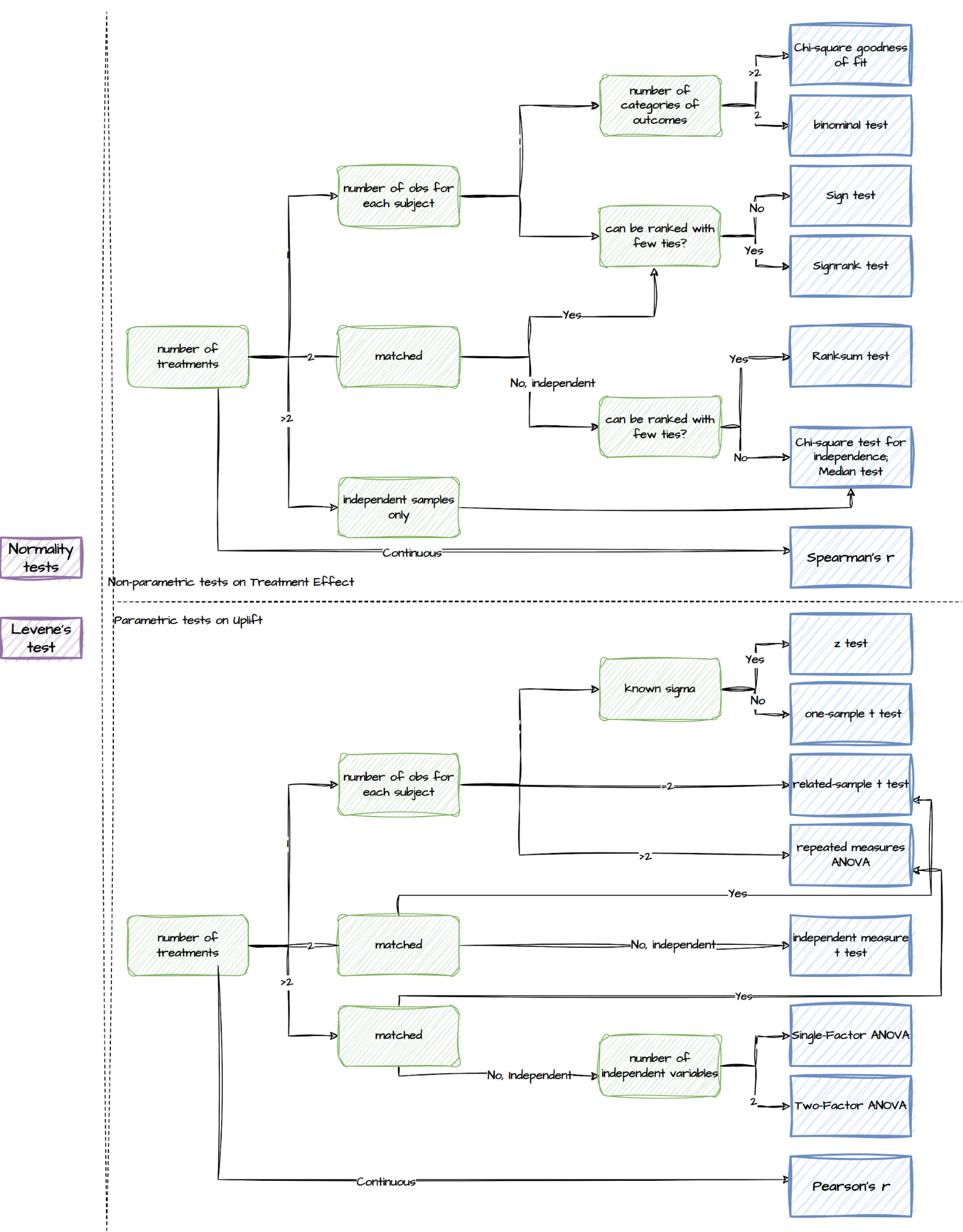
Upon completion of the experiment, a comprehensive toolbox for post-experiment analysis is available. This toolbox consists of a wide range of statistical tests, ranging from normality tests to non-parametric and parametric tests. Here is an overview of the different types of tests included in the toolbox for different experiment setups:
Tests supported by the post-experiment analysis component
Though we make all the relevant tests available, the package sets a default list of output. With just two lines of code specifying the desired experiment design, experimenters can easily retrieve the recommended results, as summarised in the following table.
Types
Details
Basic statistics
The mean, variance, and sample size of Treatment and Control
Uplift tests
Welch’s t-test; Non-parametric tests, such as Wilcoxon signed-rank test and Mann-Whitney U Test
Misc tests
Normality tests such as the Shapiro-Wilk test, Anderson-Darling test, and Kolmogorov-Smirnov test; Levene test which assesses the equality of variances between groups
Regression models
A standard OLS/Logit model to estimate the treatment uplift; Recommended regression models
Warning
Provides a warning or notification related to the statistical analysis or results, for example: – Lack of variation in the variables – Sample size is too small – Too few randomisation units which will lead to under-estimated standard errors
Recommended regression models
Besides reporting relevant statistical test results, we adopt regression models to leverage their flexibility in controlling for confounders, fixed effects and heteroskedasticity, as is commonly observed in our experiments. As mentioned in the section “A note on experimental design”, each approach has different implications on the achieved randomisation, and hence requires its own customised regression models.
Between-subject design: the observations are not independent and identically distributed (i.i.d) but clustered due to repeated observations of the same experimental units. Therefore, we set the default clustering level at the participant level in our regression models, considering that most of our between-subject experiments only take a small portion of the population (Abadie et al., 2022).
Within-subject design: this has further challenges, including spillover effects and randomisation imbalances. As a result, they often require better control of confounding factors. We adopt panel data methods and impose time fixed effects, with no option to remove them. Though users have the flexibility to define these themselves, we use hourly fixed effects as our default as we have found that these match the typical seasonality we observe in marketplace metrics. Similar to between-subject
designs, we use standard error corrections for clustered errors, and small number of clusters, as the default. Our API is flexible for users to include further controls, as well as further fixed effects to adapt the estimator to geo-timeslice designs.
Advanced tools
Apart from the pre-experiment Trusted Advisor and the post-experiment Analysis Toolbox, we have enriched this package by providing more advanced tools. Some of them are set as a default feature in the previous two components, while others are ad-hoc capabilities which the users can utilise via calling the functions directly.
Variance reduction
We bring in multiple methods to reduce variance and improve the power and sensitivity of experiments:
Stratified sampling: recognised for reducing variance during assignment
Post stratification: a post-assignment variance reduction technique
MLRATE: an extension of CUPED that allows for the use of non-linear / machine learning models
These approaches offer valuable ways to mitigate variance and improve the overall effectiveness of experiments. The experimenters can directly access these ad hoc capabilities via the package.
Multiple comparisons problem
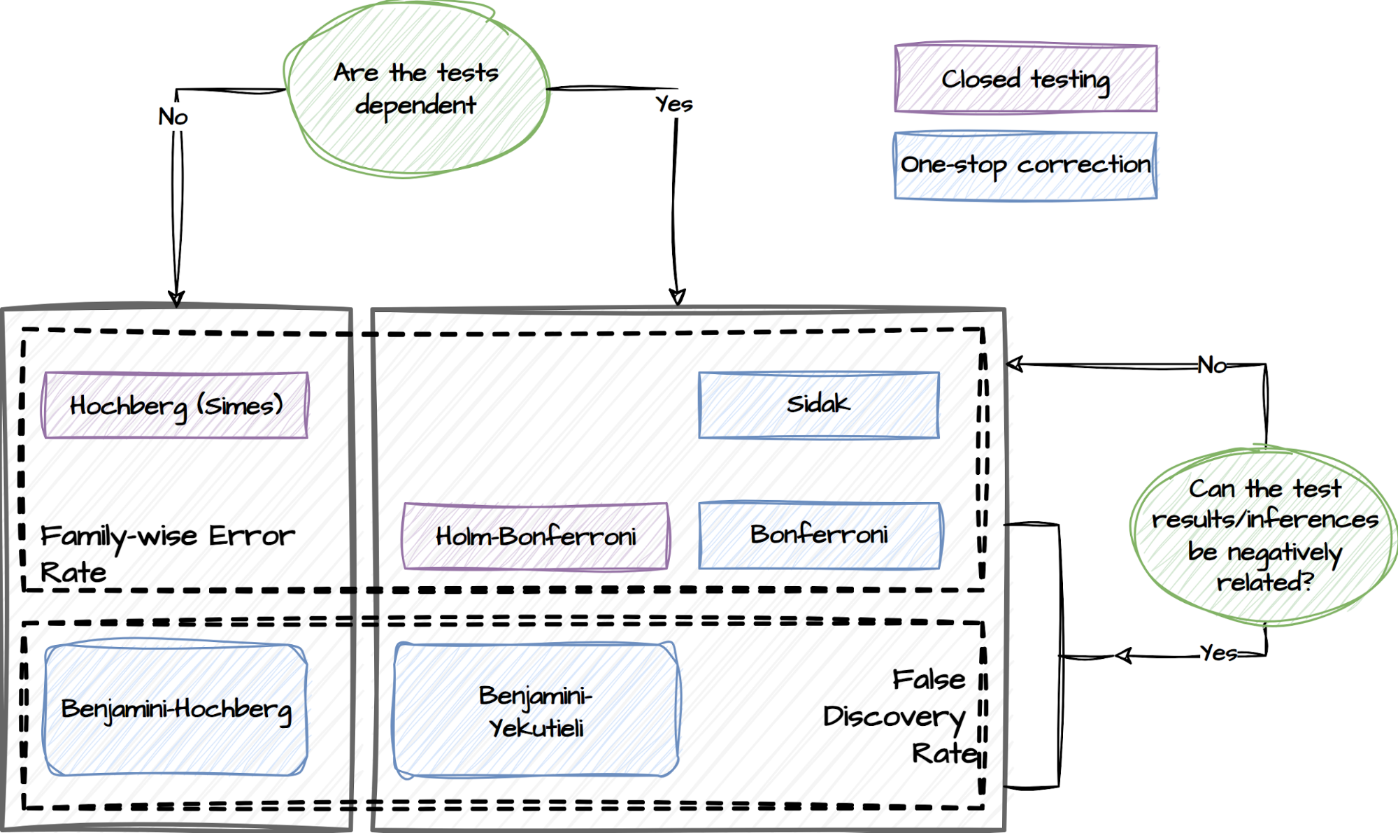
A multiple comparisons problem occurs when multiple hypotheses are simultaneously tested, leading to a higher likelihood of false positives. To address this, we implement various statistical correction techniques in this package, as illustrated below.
Statistical correction techniques
Experimenters can specify if they have concerns about the dependency of the tests and whether the test results are expected to be negatively related. This capability will adopt the following procedures and choose the relevant tests to mitigate the risk of false positives accordingly:
False Discovery Rate (FDR) procedures, which control the expected rate of false discoveries.
Family-wise Error Rate (FWER) procedures, which control the probability of making at least one false discovery within a set of related tests referred to as a family.
Multiple treatments and unequal treatment sizes
We developed a capability to deal with experiments where there are multiple treatments. This capability employs a conservative approach to ensure that the size reaches a minimum level where any pairwise comparison between the control and treatment groups has a sufficient sample size.
Heterogeneous treatment effects
Heterogeneous treatment effects refer to a situation where the treatment effect varies across different groups or subpopulations within a larger population. For instance, it may be of interest to examine treatment effects specifically on rainy days compared to non-rainy days. We have incorporated this functionality into the tests for both experiment designs. By enabling this feature, we facilitate a more nuanced analysis that accounts for potential variations in treatment effects based on different factors or contexts.
Maintenance and support
The package is available across all internal DS/Machine Learning platforms and individual local development environments within Grab. Its source code is openly accessible to all developers within Grab and its release adheres to a semantic release standard.
In addition to the technical maintenance efforts, we have introduced a dedicated committee and a workspace to address issues that may extend beyond the scope of the package’s current capabilities.
Experiment Council
Within Grab, there is a dedicated committee known as the ‘Experiment Council’. This committee includes data scientists, analysts, and economists from various functions. One of their responsibilities is to collaborate to enhance and maintain the package, as well as guide users in effectively utilising its functionalities. The Experiment Council plays a crucial role in enhancing the overall operational excellence of conducting experiments and deriving meaningful insights from them.
GrabCausal Methodology Bank
Experimenters frequently encounter challenges regarding the feasibility of conducting experiments for causal problems. To address this concern, we have introduced an alternative workspace called GrabCausal Methodology Bank. Similar to the internal open-source nature of this project, the GrabCausal Methodology bank is open to contributions from all users within Grab. It provides a collaborative space where users can readily share their code, case studies, guidelines, and suggestions related to
causal methodologies. By fostering an open and inclusive environment, this workspace encourages knowledge sharing and promotes the advancement of causal research methods.
The workspace functions as a platform, which now exhibits a wide range of commonly used methods, including Diff-in-Diff, Event studies, Regression Discontinuity Designs (RDD), Instrumental Variables (IV), Bayesian structural time series, and Bunching. Additionally, we are dedicated to incorporating more, such as Synthetic control, Double ML (Chernozhukov et al. 2018), DAG discovery/validation, etc., to further enhance our offerings in this space.
Learnings
Over the past few years, we have invested in developing and expanding this package. Our initial motivation was humble yet motivating – to contribute to improving the quality of experimentation at Grab, helping it develop from its initial start-up modus operandi to a more consolidated, rigorous, and guided approach.
Throughout this journey, we have learned that prioritisation holds the utmost significance in open-source projects of this nature; the majority of user demands can be met through relatively small yet pivotal efforts. By focusing on these core capabilities, we avoid spreading resources too thinly across all areas at the initial stage of planning and development.
Meanwhile, we acknowledge that there is still a significant journey ahead. While the package now focuses solely on individual experiments, an inherent challenge in online-controlled experimentation platforms is the interference between experiments (Gupta, et al, 2019). A recent development in the field is to embrace simultaneous tests (Microsoft, Google, Spotify and booking.com and Optimizely), and to carefully consider the tradeoff between accuracy and velocity.
The key to overcoming this challenge will be a close collaboration between the community of experimenters, the teams developing this unified toolkit, and the GrabX platform engineers. In particular, the platform developers will continue to enrich the experimentation SDK by providing diverse assignment strategies, sampling mechanisms, and user interfaces to manage potential inference risks better. Simultaneously, the community of experimenters can coordinate among themselves effectively to
avoid severe interference, which will also be monitored by GrabX. Last but not least, the development of this unified toolkit will also focus on monitoring, evaluating, and managing inter-experiment interference.
In addition, we are committed to keeping this package in sync with industry advancements. Many existing tools in this package, despite being labelled as “advanced” in the earlier discussions, are still relatively simplified. For instance,
Incorporating standard errors clustering based on the diverse assignment and sampling strategies requires attention (Abadie, et al, 2023).
Sequential testing will play a vital role in detecting uplifts earlier and safely, avoiding p-hacking. One recent innovation is the “always valid inference” (Johari, et al., 2022)
The advancements in investigating heterogeneous effects, such as Causal Forest (Athey and Wager, 2019), have extended beyond linear approaches, now incorporating nonlinear and more granular analyses.
Estimating the long-term treatment effects observed from short-term follow-ups is also a long-term objective, and one approach is using a Surrogate Index (Athey, et al 2019).
Continuous effort is required to stay updated and informed about the latest advancements in statistical testing methodologies, to ensure accuracy and effectiveness.
This article marks the beginning of our journey towards automating the experimentation and product decision-making process among the data scientist community. We are excited about the prospect of expanding the toolkit further in these directions. Stay tuned for more updates and posts.
References
Abadie, Alberto, et al. “When should you adjust standard errors for clustering?.” The Quarterly Journal of Economics 138.1 (2023): 1-35.
Athey, Susan, et al. “The surrogate index: Combining short-term proxies to estimate long-term treatment effects more rapidly and precisely.” No. w26463. National Bureau of Economic Research, 2019.
Athey, Susan, and Stefan Wager. “Estimating treatment effects with causal forests: An application.” Observational studies 5.2 (2019): 37-51.
Chernozhukov, Victor, et al. “Double/debiased machine learning for treatment and structural parameters.” (2018): C1-C68.
Facure, Matheus. Causal Inference in Python. O’Reilly Media, Inc., 2023.
Gupta, Somit, et al. “Top challenges from the first practical online controlled experiments summit.” ACM SIGKDD Explorations Newsletter 21.1 (2019): 20-35.
Huntington-Klein, Nick. The Effect: An Introduction to Research Design and Causality. CRC Press, 2021.
Imbens, Guido W. and Donald B. Rubin. Causal Inference for Statistics, Social, and Biomedical Sciences: An Introduction. Cambridge University Press, 2015.
Johari, Ramesh, et al. “Always valid inference: Continuous monitoring of a/b tests.” Operations Research 70.3 (2022): 1806-1821.
List, John A., Sally Sadoff, and Mathis Wagner. “So you want to run an experiment, now what? Some simple rules of thumb for optimal experimental design.” Experimental Economics 14 (2011): 439-457.
Moffatt, Peter. Experimetrics: Econometrics for Experimental Economics. Bloomsbury Publishing, 2020.
Join us
Grab is the leading superapp platform in Southeast Asia, providing everyday services that matter to consumers. More than just a ride-hailing and food delivery app, Grab offers a wide range of on-demand services in the region, including mobility, food, package and grocery delivery services, mobile payments, and financial services across 428 cities in eight countries.
Powered by technology and driven by heart, our mission is to drive Southeast Asia forward by creating economic empowerment for everyone. If this mission speaks to you, join our team today!
Have you ever encountered a bug while streaming Netflix? Did your title stop unexpectedly, or not start at all? In the first installment of this blog series on sequential testing, we described our canary testing methodology for continuous metrics such as play-delay. One of our readers commented
What if the new release is not related to a new play/streaming feature? For example, what if the new release includes modified login functionality? Will you still monitor the “play-delay” metric?
Netflix monitors a large suite of metrics, many of which can be classified as counts. These include metrics such as the number of logins, errors, successful play starts, and even the number of customer call center contacts. In this second installment, we describe our sequential methodology for testing count metrics, outlined in the NeurIPS paper Anytime Valid Inference for Multinomial Count Data.
Spot the Difference
Suppose we are about to deploy new code that changes the login behavior. To de-risk the software rollout we A/B test the new code, known also as a canary test. Whenever an event such as a login occurs, a log flows through our real-time backend and the corresponding timestamp is recorded. Figure 1 illustrates the sequences of timestamps generated by devices assigned to the new (treatment) and existing (control) software versions. A question that naturally concerns us is whether there are fewer login events in the treatment. Can you tell?
Figure 1: Timestamps of events occurring in control and treatment
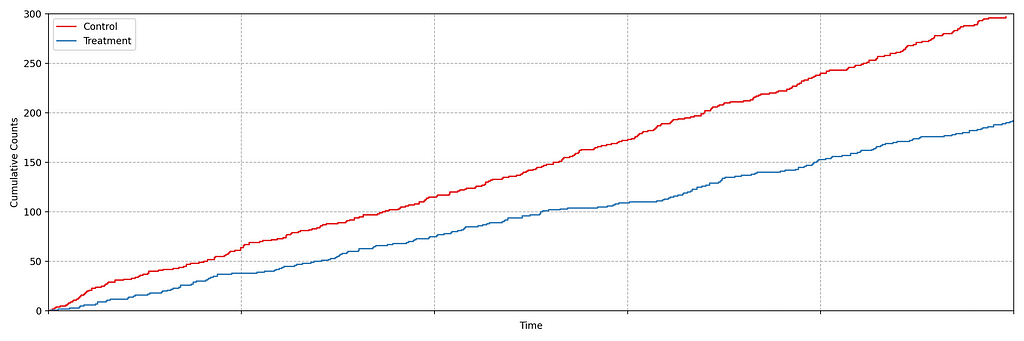
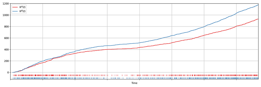
It is not immediately obvious by simple inspection of the point processes in Figure 1. The difference becomes immediately obvious when we visualize the observed counting processes, shown in Figure 2.
Figure 2: Visualizing the counting processes — the number of events observed by time t
The counting processes are functions that increment by 1 whenever a new event arrives. Clearly, there are fewer events occurring in the treatment than in the control. If these were login events, this would suggest that the new code contains a bug that prevents some users from being able to log in successfully.
This is a common situation when dealing with event timestamps. To give another example, if events corresponded to errors or crashes, we would like to know if these are accruing faster in the treatment than in the control. Moreover, we want to answer that question as quickly as possible to prevent any further disruption to the service. This necessitates sequential testing techniques which were introduced in part 1.
Time-Inhomogeneous Poisson Process
Our data for each treatment group is a realization of a one-dimensional point process, that is, a sequence of timestamps. As the rate at which the events arrive is time-varying (in both treatment and control), we model the point process as a time-inhomogeneous Poisson point process. This point process is defined by an intensity function λ: ℝ → [0, ∞). The number of events in the interval [0,t), denoted N(t), has the following Poisson distribution
N(t) ~ Poisson(Λ(t)), where Λ(t) = ∫₀ᵗ λ(s) ds.
We seek to test the null hypothesis H₀: λᴬ(t) = λᴮ(t) for all t i.e. the intensity functions for control (A) and treatment (B) are the same. This can be done semiparametrically without making any assumptions about the intensity functions λᴬ and λᴮ. Moreover, the novelty of the research is that this can be done sequentially, as described in section 4 of our paper. Conveniently, the only data required to test this hypothesis at time t is Nᴬ(t) and Nᴮ(t), the total number of events observed so far in control and treatment. In other words, all you need to test the null hypothesis is two integers, which can easily be updated as new events arrive. Here is an example from a simulated A/A test, in which we know by design that the intensity function is the same for the control (A) and the treatment (B), albeit nonstationary.
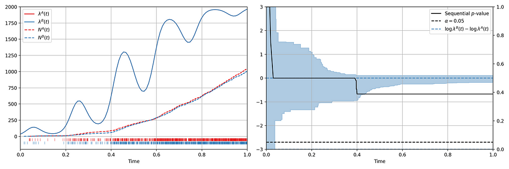
Figure 3: (Left) An A/A simulation of two inhomogeneous Poisson point processes. (Right) Confidence sequence on the log-difference of intensity functions, and sequential p-value.
Figure 3 provides an illustration of an A/A setting. The left figure presents the raw data and the intensity functions, and the right figure presents the sequential statistical analysis. The blue and red rug plots indicate the observed arrival timestamps of events from the treatment and control streams respectively. The dashed lines are the observed counting processes. As this data is simulated under the null, the intensity functions are identical and overlay each other. The left axis of the right figure visualizes the evolution of the confidence sequence on the log-difference of intensity functions. The right axis of the right figure visualizes the evolution of the sequential p-value. We can make the two following observations
Under the null, the difference of log intensities is zero, which is correctly covered by the 0.95 confidence sequence at all times.
The sequential p-value is greater than 0.05 at all times
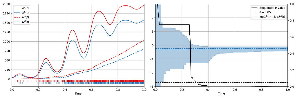
Now let’s consider an illustration of an A/B setting. Figure 4 shows observed arrival times for treatment and control when the intensity functions differ. As this is a simulation, the true difference between log intensities is known.
Figure 4: (Left) An A/B simulation of two inhomogeneous Poisson point processes. (Right) Confidence sequence on the difference of log of intensity functions, and sequential p-value.
We can make the following observations
The 0.95 confidence sequence covers the true log-difference at all times
The sequential p-value falls below 0.05 at the same time the 0.95 confidence sequence excludes the null value of zero
Now we present a number of case studies where this methodology has rapidly detected serious problems in a number of count metrics
Case Study 1: Drop in Successful Title Starts
Figure 2 actually presents counts of title start events from a real canary test. Whenever a title starts successfully, an event is sent from the device to Netflix. We have a stream of title start events from treatment devices and a stream of title start events from control devices. Whenever fewer title starts are observed among treatment devices, there is usually a bug in the new client preventing playback.
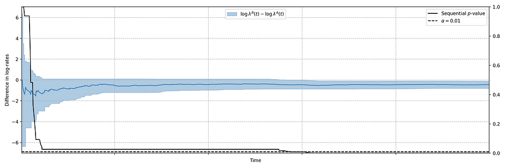
In this case, the canary test detected a bug that was later determined to have prevented approximately 60% of treatment devices from being able to start their streams. The confidence sequence is shown in Figure 5, in addition to the (sequential) p-value. While the exact units of time have been omitted, this bug was detected at the sub-second level.
Figure 5: 0.99 Confidence sequence on the difference of log-intensities with sequential p-value.
Case Study 2: Increase in Abnormal Shutdowns
In addition to title start events, we also monitor whenever the Netflix client shuts down unexpectedly. As before, we have two streams of abnormal shutdown events, one from treatment devices, and one from control devices. The following screenshots are taken directly from our Lumen dashboards.
Figure 6: Counts of Abnormal Shutdowns over time, cumulative and non-cumulative. Treatment (Black) and Control (Blue)
Figure 6 illustrates two important points. There is clearly nonstationarity in the arrival of abnormal shutdown events. It is also not easy to visibly see any difference between treatment and control from the non-cumulative view. The difference is, however, much easier to see from the cumulative view by observing the counting process. There is a small but visible increase in the number of abnormal shutdowns in the treatment. Figure 7 shows how our sequential statistical methodology is even able to identify such small differences.
Figure 7: Abnormal Shutdowns. (Top Panel) Confidence sequences on λᴮ(t)/λᴬ(t) (shaded blue) with observed counting processes for treatment (black dashed) and control (blue dashed). (Bottom Panel) sequential p-values.
Case Study 3: Increase in Errors
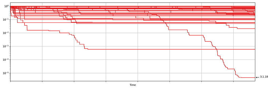
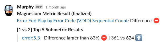
Netflix also monitors the number of errors produced by treatment and control. This is a high cardinality metric as every error is annotated with a code indicating the type of error. Monitoring errors segmented by code helps developers diagnose issues quickly. Figure 8 shows the sequential p-values, on the log scale, for a set of error codes that Netflix monitors during client rollouts. In this example, we have detected a higher volume of 3.1.18 errors being produced by treatment devices. Devices experiencing this error are presented with the following message:
“We’re having trouble playing this title right now”
Figure 8: Sequential p-values for start play errors by error codeFigure 9: Observed error-3.1.18 timestamps and counting processes for treatment (blue) and control (red)
Knowing which errors increased can streamline the process of identifying the bug for our developers. We immediately send developers alerts through Slack integrations, such as the following
Figure 10: Notifications via Slack Integrations
The next time you are watching Netflix and encounter an error, know that we’re on it!
Try it Out!
The statistical approach outlined in our paper is remarkably easy to implement in practice. All you need are two integers, the number of events observed so far in the treatment and control. The code is available in this short GitHub gist. Here are two usage examples:
Can you spot any difference between the two data streams below? Each observation is the time interval between a Netflix member hitting the play button and playback commencing, i.e., play-delay. These observations are from a particular type of A/B test that Netflix runs called a software canary or regression-driven experiment. More on that below — for now, what’s important is that we want to quickly and confidently identify any difference in the distribution of play-delay — or conclude that, within some tolerance, there is no difference.
In this blog post, we will develop a statistical procedure to do just that, and describe the impact of these developments at Netflix. The key idea is to switch from a “fixed time horizon” to an “any-time valid” framing of the problem.
Figure 1. An example data stream for an A/B test where each observation represents play-delay for the control (left) and treatment (right). Can you spot any differences in the statistical distributions between the two data streams?
2. Safe software deployment, canary testing, and play-delay
Software engineering readers of this blog are likely familiar with unit, integration and load testing, as well as other testing practices that aim to prevent bugs from reaching production systems. Netflix also performs canary tests — software A/B tests between current and newer software versions. To learn more, see our previous blog post on Safe Updates of Client Applications.
The purpose of a canary test is twofold: to act as a quality-control gate that catches bugs prior to full release, and to measure performance of the new software in the wild. This is carried out by performing a randomized controlled experiment on a small subset of users, where the treatment group receives the new software update and the control group continues to run the existing software. If any bugs or performance regressions are observed in the treatment group, then the full-scale release can be prevented, limiting the “impact radius” among the user base.
One of the metrics Netflix monitors in canary tests is how long it takes for the video stream to start when a title is requested by a user. Monitoring this “play-delay” metric throughout releases ensures that the streaming performance of Netflix only ever improves as we release newer versions of the Netflix client. In Figure 1, the left side shows a real-time stream of play-delay measurements from users running the existing version of the Netflix client, while the right side shows play-delay measurements from users running the updated version. We ask ourselves: Are users of the updated client experiencing longer play-delays?
We consider any increase in play-delay to be a serious performance regression and would prevent the release if we detect an increase. Critically, testing for differences in means or medians is not sufficient and does not provide a complete picture. For example, one situation we might face is that the median or mean play-delay is the same in treatment and control, but the treatment group experiences an increase in the upper quantiles of play-delay. This corresponds to the Netflix experience being degraded for those who already experience high play delays — likely our members on slow or unstable internet connections. Such changes should not be ignored by our testing procedure.
For a complete picture, we need to be able to reliably and quickly detect an upward shift in any part of the play-delay distribution. That is, we must do inference on and test for any differences between the distributions of play-delay in treatment and control.
To summarize, here are the design requirements of our canary testing system:
Identify bugs and performance regressions, as measured by play-delay, as quickly as possible. Rationale: To minimize member harm, if there is any problem with the streaming quality experienced by users in the treatment group we need to abort the canary and roll back the software change as quickly as possible.
Strictly control false positive (false alarm) probabilities. Rationale: This system is part of a semi-automated process for all client deployments. A false positive test unnecessarily interrupts the software release process, reducing the velocity of software delivery and sending developers looking for bugs that do not exist.
This system should be able to detect any change in the distribution. Rationale: We care not only about changes in the mean or median, but also about changes in tail behaviour and other quantiles.
We now build out a sequential testing procedure that meets these design requirements.
3. Sequential Testing: The Basics
Standard statistical tests are fixed-n or fixed-time horizon: the analyst waits until some pre-set amount of data is collected, and then performs the analysis a single time. The classic t-test, the Kolmogorov-Smirnov test, and the Mann-Whitney test are all examples of fixed-n tests. A limitation of fixed-n tests is that they can only be performed once — yet in situations like the above, we want to be testing frequently to detect differences as soon as possible. If you apply a fixed-n test more than once, then you forfeit the Type-I error or false positive guarantee.
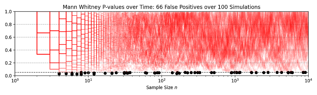
Here’s a quick illustration of how fixed-n tests fail under repeated analysis. In the following figure, each red line traces out the p-value when the Mann-Whitney test is repeatedly applied to a data set as 10,000 observations accrue in both treatment and control. Each red line shows an independent simulation, and in each case, there is no difference between treatment and control: these are simulated A/A tests.
The black dots mark where the p-value falls below the standard 0.05 rejection threshold. An alarming 70% of simulations declare a significant difference at some point in time, even though, by construction, there is no difference: the actual false positive rate is much higher than the nominal 0.05. Exactly the same behaviour would be observed for the Kolmogorov-Smirnov test.
Figure 2. 100 Sample paths of the p-value process simulated under the null hypothesis shown in red. The dotted black line indicates the nominal alpha=0.05 level. Black dots indicate where the p-value process dips below the alpha=0.05 threshold, indicating a false rejection of the null hypothesis. A total of 66 out of 100 A/A simulations falsely rejected the null hypothesis.
This is a manifestation of “peeking”, and much has been written about the downside risks of this practice (see, for example, Johari et al. 2017). If we restrict ourselves to correctly applied fixed-n statistical tests, where we analyze the data exactly once, we face a difficult tradeoff:
Perform the test early on, after a small amount of data has been collected. In this case, we will only be powered to detect larger regressions. Smaller performance regressions will not be detected, and we run the risk of steadily eroding the member experience as small regressions accrue.
Perform the test later, after a large amount of data has been collected. In this case, we are powered to detect small regressions — but in the case of large regressions, we expose members to a bad experience for an unnecessarily long period of time.
Sequential, or “any-time valid”, statistical tests overcome these limitations. They permit for peeking –in fact, they can be applied after every new data point arrives– while providing false positive, or Type-I error, guarantees that hold throughout time. As a result, we can continuously monitor data streams like in the image above, using confidence sequences or sequential p-values, and rapidly detect large regressions while eventually detecting small regressions.
Despite relatively recent adoption in the context of digital experimentation, these methods have a long academic history, with initial ideas dating back to Abraham Wald’s Sequential Tests of Statistical Hypothesesfrom 1945. Research in this area remains active, and Netflix has made a number of contributions in the last few years (see the references in these papers for a more complete literature review):
In this and following blogs, we will describe both the methods we’ve developed and their applications at Netflix. The remainder of this post discusses the first paper above, which was published at KDD ’22 (and available on ArXiV). We will keep it high level — readers interested in the technical details can consult the paper.
4. A sequential testing solution
Differences in Distributions
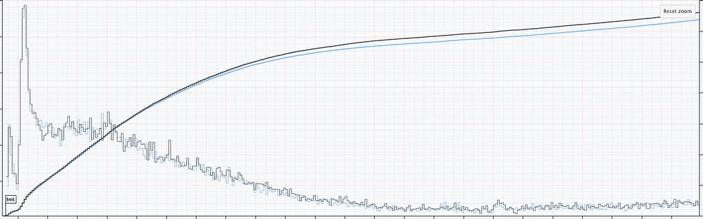
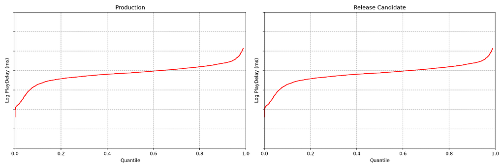
At any point in time, we can estimate the empirical quantile functions for both treatment and control, based on the data observed so far.
Figure 3: Empirical quantile function for control (left) and treatment (right) at a snapshot in time after starting the canary experiment. This is from actual Netflix data, so we’ve suppressed numerical values on the y-axis.
These two plots look pretty close, but we can do better than an eyeball comparison — and we want the computer to be able to continuously evaluate if there is any significant difference between the distributions. Per the design requirements, we also wish to detect large effects early, while preserving the ability to detect small effects eventually — and we want to maintain the false positive probability at a nominal level while permitting continuous analysis (aka peeking).
That is, we need a sequential test on the difference in distributions.
Obtaining “fixed-horizon” confidence bands for the quantile function can be achieved using the DKWM inequality. To obtain time-uniform confidence bands, however, we use the anytime-valid confidence sequences from Howard and Ramdas (2022) [arxiv version]. As the coverage guarantee from these confidence bands holds uniformly across time, we can watch them become tighter without being concerned about peeking. As more data points stream in, these sequential confidence bands continue to shrink in width, which means any difference in the distribution functions — if it exists — will eventually become apparent.
Figure 4: 97.5% Time-Uniform Confidence bands on the quantile function for control (left) and treatment (right)
Note each frame corresponds to a point in time after the experiment began, not sample size. In fact, there is no requirement that each treatment group has the same sample size.
Differences are easier to see by visualizing the difference between the treatment and control quantile functions.
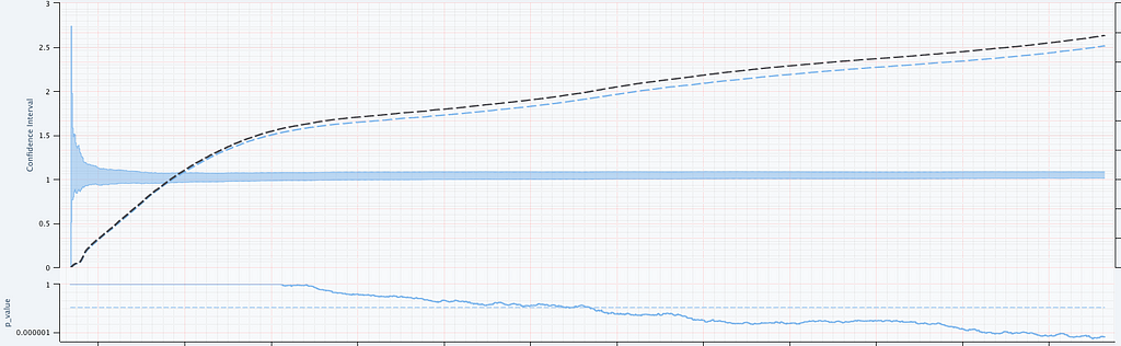
Figure 5: 95% Time-Uniform confidence band on the quantile difference function Q_b(p) — Q_a(p) (left). The sequential p-value (right).
As the sequential confidence band on the treatment effect quantile function is anytime-valid, the inference procedure becomes rather intuitive. We can continue to watch these confidence bands tighten, and if at any point the band no longer covers zero at any quantile, we can conclude that the distributions are different and stop the test. In addition to the sequential confidence bands, we can also construct a sequential p-value for testing that the distributions differ. Note from the animation that the moment the 95% confidence band over quantile treatment effects excludes zero is the same moment that the sequential p-value falls below 0.05: as with fixed-n tests, there is consistency between confidence intervals and p-values.
There are many multiple testing concerns in this application. Our solution controls Type-I error across all quantiles, all treatment groups, and all joint sample sizes simultaneously (see our paper, or Howard and Ramdas for details). Results hold for all quantiles, and for all times.
5. Impact at Netflix
Releasing new software always carries risk, and we always want to reduce the risk of service interruptions or degradation to the member experience. Our canary testing approach is another layer of protection for preventing bugs and performance regressions from slipping into production. It’s fully automated and has become an integral part of the software delivery process at Netflix. Developers can push to production with peace of mind, knowing that bugs and performance regressions will be rapidly caught. The additional confidence empowers developers to push to production more frequently, reducing the time to market for upgrades to the Netflix client and increasing our rate of software delivery.
So far this system has successfully prevented a number of serious bugs from reaching our end users. We detail one example.
Case study: Safe Rollout of Netflix Client Application
Figures 3–5 are taken from a canary test in which the behaviour of the client application was modified application (actual numerical values of play-delay have been suppressed). As we can see, the canary test revealed that the new version of the client increases a number of quantiles of play-delay, with the median and 75% percentile of play experiencing relative increases of at least 0.5% and 1% respectively. The timeseries of the sequential p-value shows that, in this case, we were able to reject the null of no change in distribution at the 0.05 level after about 60 seconds. This provides rapid feedback in the software delivery process, allowing developers to test the performance of new software and quickly iterate.
6. What’s next?
If you are curious about the technical details of the sequential tests for quantiles developed here, you can learn all about the math in our KDD paper (also available on arxiv).
You might also be wondering what happens if the data are not continuous measurements. Errors and exceptions are critical metrics to log when deploying software, as are many other metrics which are best defined in terms of counts. Stay tuned — our next post will develop sequential testing procedures for count data.
In Grab, the Trust, Identity, Safety, and Security (TISS) is a team of software engineers and AI developers working on fraud detection, login identity check, safety issues, etc. There are many TISS services, like grab-fraud, grab-safety, and grab-id. They make billions of business decisions daily using the Griffin rule engine, which determines if a passenger can book a trip, get a food promotion, or if a driver gets a delivery booking.
There is a natural demand to log down all these important business decisions, store them and query them interactively or in batches. Data analysts and scientists need to use the data to train their machine learning models. RiskOps and customer service teams can query the historical data and help consumers.
That’s where Archivist comes in; it is a new tracing, statistics and feedback system for rule and machine learning-based predictions. It is reliable and performant. Its innovative data schema is flexible for storing events from different business scenarios. Finally, it provides a user-friendly UI, which has access control for classified data.
Here are the impacts Archivist has already made:
Currently, there are 2 teams with a total of 5 services and about 50 business scenarios using Archivist. The scenarios include fraud prevention (e.g. DriverBan, PassengerBan), payment checks (e.g. PayoutBlockCheck, PromoCheck), and identity check events like PinTrigger.
It takes only a few minutes to onboard a new business scenario (event type), by using the configuration page on the user portal. Previously, it took at least 1 to 2 days.
Each day, Archivist logs down 80 million logs to the ElasticSearch cluster, which is about 200GB of data.
Each week, Customer Experience (CE)/Risk Ops goes to the user portal and checks Archivist logs for about 2,000 distinct customers. They can search based on numerous dimensions such as the Passenger/DriverID, phone number, request ID, booking code and payment fingerprint.
Background
Each day, TISS services make billions of business decisions (predictions), based on the Griffin rule engine and ML models.
After the predictions are made, there are still some tough questions for these services to answer.
If Risk Ops believes a prediction is false-positive, a consumer could be banned. If this happens, how can consumers or Risk Ops report or feedback this information to the new rule and ML model training quickly?
As CustomService/Data Scientists investigating any tickets opened due to TISS predictions/decisions, how do you know which rules and data were used? E.g. why the passenger triggered a selfie, or why a booking was blocked.
After Data Analysts/Data Scientists (DA/DS) launch a new rule/model, how can they track the performance in fine-granularity and in real-time? E.g. week-over-week rule performance in a country or city.
How can DA/DS access all prediction data for data analysis or model training?
How can the system keep up with Grab’s business launch speed, with maximum self-service?
Problem
To answer the questions above, TISS services previously used company-wide Kibana to log predictions. For example, a log looks like: PassengerID:123,Scenario:PinTrigger,Decision:Trigger,.... This logging method had some obvious issues:
Logs in plain text don’t have any structure and are not friendly to ML model training as most ML models need processed data to make accurate predictions.
Furthermore, there is no fine-granularity access control for developers in Kibana.
Developers, DA and DS have no access control while CEs have no access at all. So CE cannot easily see the data and DA/DS cannot easily process the data.
To address all the Kibana log issues, we developed ActionTrace, a code library with a well-structured data schema. The logs, also called documents, are stored in a dedicated ElasticSearch cluster with access control implemented. However, after using it for a while, we found that it still needed some improvements.
Each business scenario involves different types of entities and ActionTrace is not fully self-service. This means that a lot of development work was needed to support fast-launching business scenarios. Here are some examples:
The main entities in the taxi business are Driver and Passenger,
The main entities in the food business can be Merchant, Driver and Consumer.
All these entities will need to be manually added into the ActionTrace data schema.
Each business scenario may have their own custom information logged. Because there is no overlap, each of them will correspond to a new field in the data schema. For example:
For any scenario involving payment, a valid payment method and expiration date is logged.
For the taxi business, the geohash is logged.
To store the log data from ActionTrace, different teams need to set up and manage their own ElasticSearch clusters. This increases hardware and maintenance costs.
There was a simple Web UI created for viewing logs from ActionTrace, but there was still no access control in fine granularity.
Solution
We developed Archivist, a new tracing, statistics, and feedback system for ML/rule-based prediction events. It’s centralised, performant and flexible. It answers all the issues mentioned above, and it is an improvement over all the existing solutions we have mentioned previously.
The key improvements are:
User-defined entities and custom fields
There are no predefined entity types. Users can define up to 5 entity types (E.g. PassengerId, DriverId, PhoneNumber, PaymentMethodId, etc.).
Similarly, there are a limited number of custom data fields to use, in addition to the common data fields shared by all business scenarios.
A dedicated service shared by all other services
Each service writes its prediction events to a Kafka stream. Archivist then reads the stream and writes to the ElasticSearch cluster.
The data writes are buffered, so it is easy to handle traffic surges in peak time.
Different services share the same Elastic Cloud Enterprise (ECE) cluster, but they create their own daily file indices so the costs can be split fairly.
Better support for data mining, prediction stats and feedback
Kafka stream data are simultaneously written to AWS S3. DA/DS can use the PrestoDB SQL query engine to mine the data.
There is an internal web portal for viewing Archivist logs. Customer service teams and Ops can use no-risk data to address CE tickets, while DA, DS and developers can view high-risk data for code/rule debugging.
A reduction of development days to support new business launches
Previously, it took a week to modify and deploy the ActionTrace data schema. Now, it only takes several minutes to configure event schemas in the user portal.
Saves time in RiskOps/CE investigations
With the new web UI which has access control in place, the different roles in the company, like Customer service and Data analysts, can access the Archivist events with different levels of permissions.
It takes only a few clicks for them to find the relevant events that impact the drivers/passengers.
Architecture Details
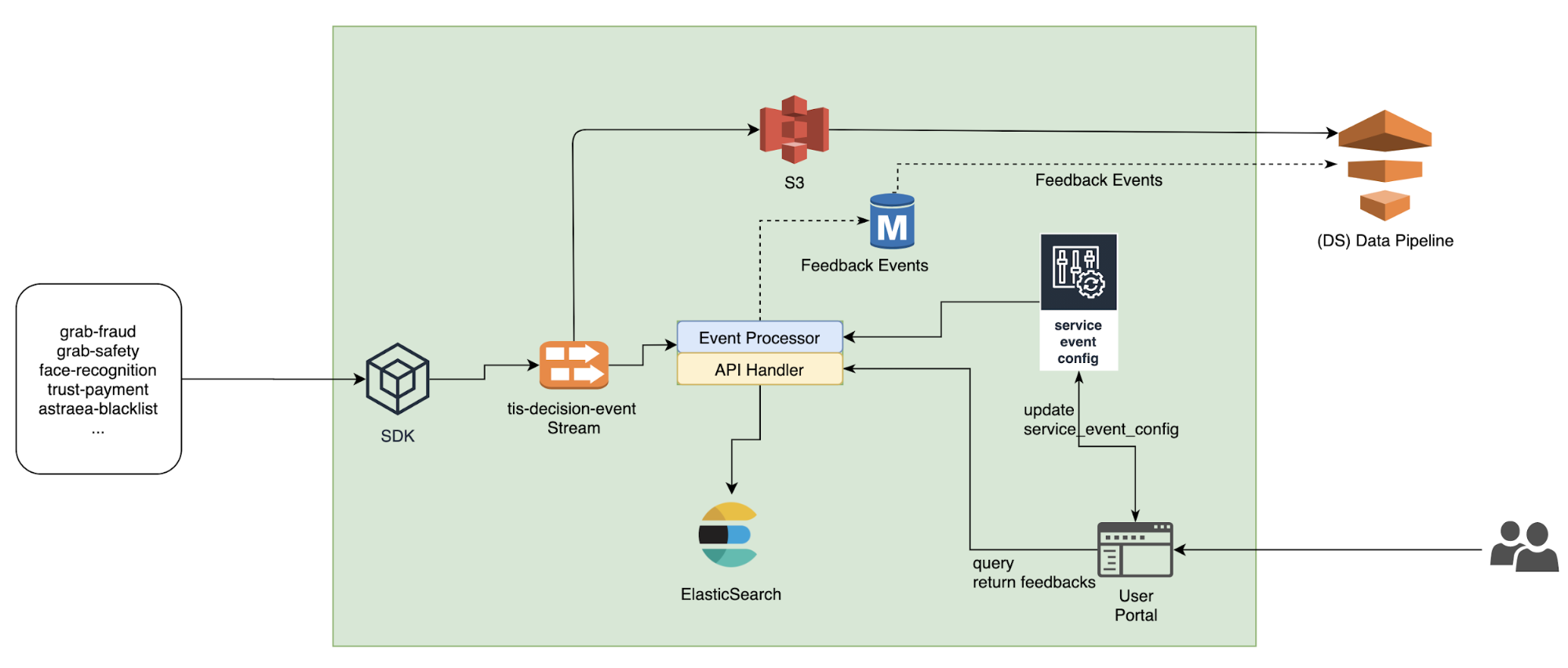
Archivist’s system architecture is shown in the diagram below.
Archivist system architecture
Different services (like fraud-detection, safety-allocation, etc.) use a simple SDK to write data to a Kafka stream (the left side of the diagram).
In the centre of Archivist is an event processor. It reads data from Kafka, and writes them to ElasticSearch (ES).
The Kafka stream writes to the Amazon S3 data lake, so DA/DS can use the Presto SQL query engine to query them.
The user portal (bottom right) can be used to view the Archivist log and update configurations. It also sends all the web requests to the API Handler in the centre.
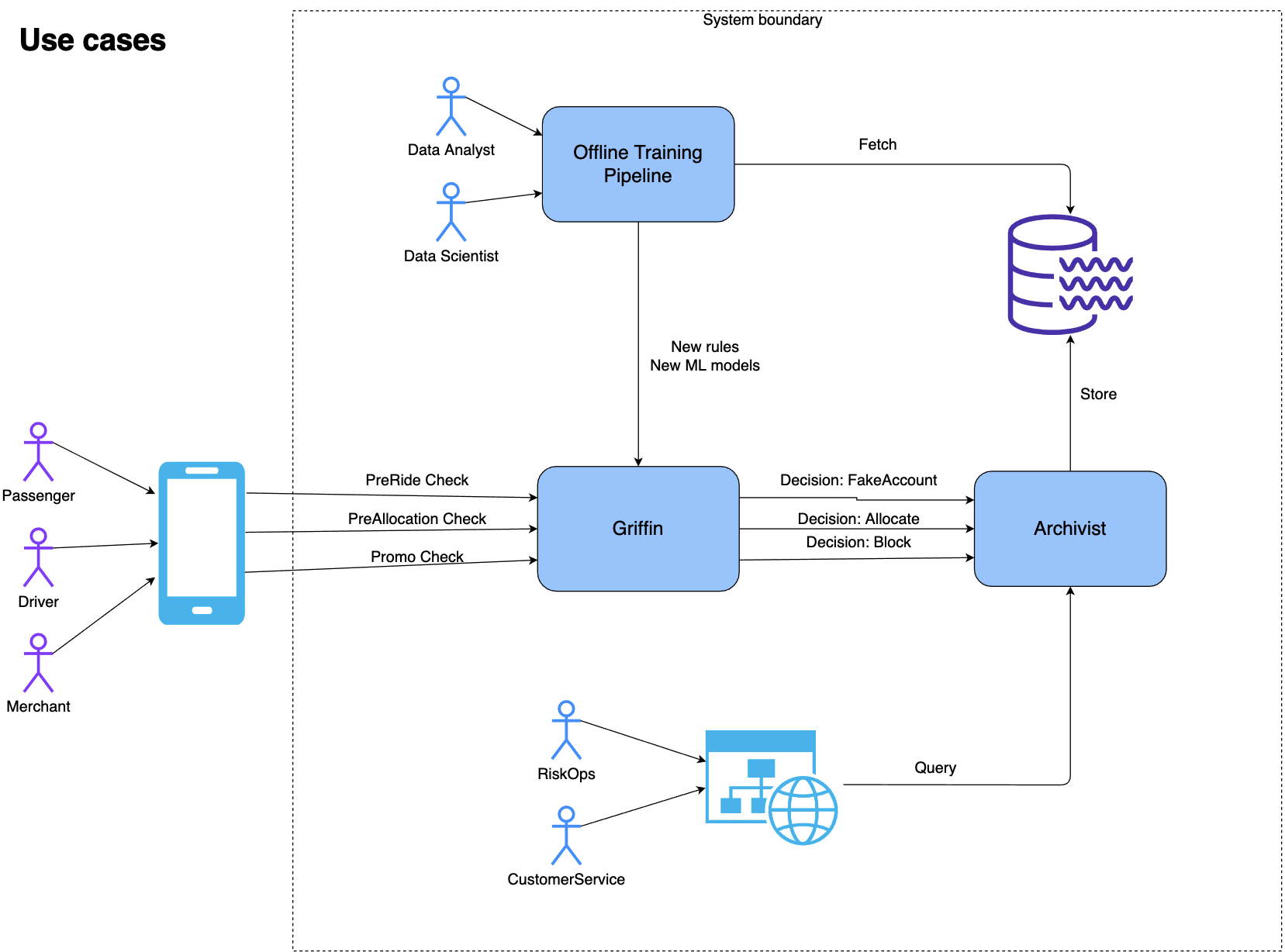
The following diagram shows how internal and external users use Archivist as well as the interaction between the Griffin rule engine and Archivist.
Archivist use cases
Flexible Event Schema
In Archivist, a prediction/decision is called an event. The event schema can be divided into 3 main parts conceptually.
Data partitioning: Fields like service_name and event_type categorise data by services and business scenarios.
Field name
Type
Example
Notes
service_name
string
GrabFraud
Name of the Service
event_type
string
PreRide
PaxBan/SafeAllocation
Business decision making: request_id, decisions, reasons, event_content are used to record the business decision, the reason and the context (E.g. The input features of machine learning algorithms).
Field name
Type
Example
Notes
request_id
string
a16756e8-efe2-472b-b614-ec6ae08a5912
a 32-digit id for web requests
event_content
string
Event context
decisions
[string]
[“NotAllowBook”, “SMS”]
A list
reasons
string
json payload string of the response from engine.
Customisation: Archivist provides user-defined entities and custom fields that we feel are sufficient and flexible for handling different business scenarios.
Field name
Type
Example
Notes
entity_type_1
string
Passenger
entity_id_1
string
12151
entity_type_2
string
Driver
entity_id_2
string
341521-rdxf36767
…
string
entity_id_5
string
custom_field_type_1
string
“MessageToUser”
custom_field_1
string
“please contact Ops”
User defined fields
custom_field_type_2
“Prediction rule:”
custom_field_2
string
“ML rule: 123, version:2”
…
string
custom_field_6
string
A User Portal to Support Querying, Prediction Stats and Feedback
DA, DS, Ops and CE can access the internal user portal to see the prediction events, individually and on an aggregated city level.
A snapshot of the Archivist logs showing the aggregation of the data in each city
There are graphs on the portal, showing the rule/model performance on individual customers over a period of time.
Rule performance on a customer over a period of time
How to Use Archivist for Your Service
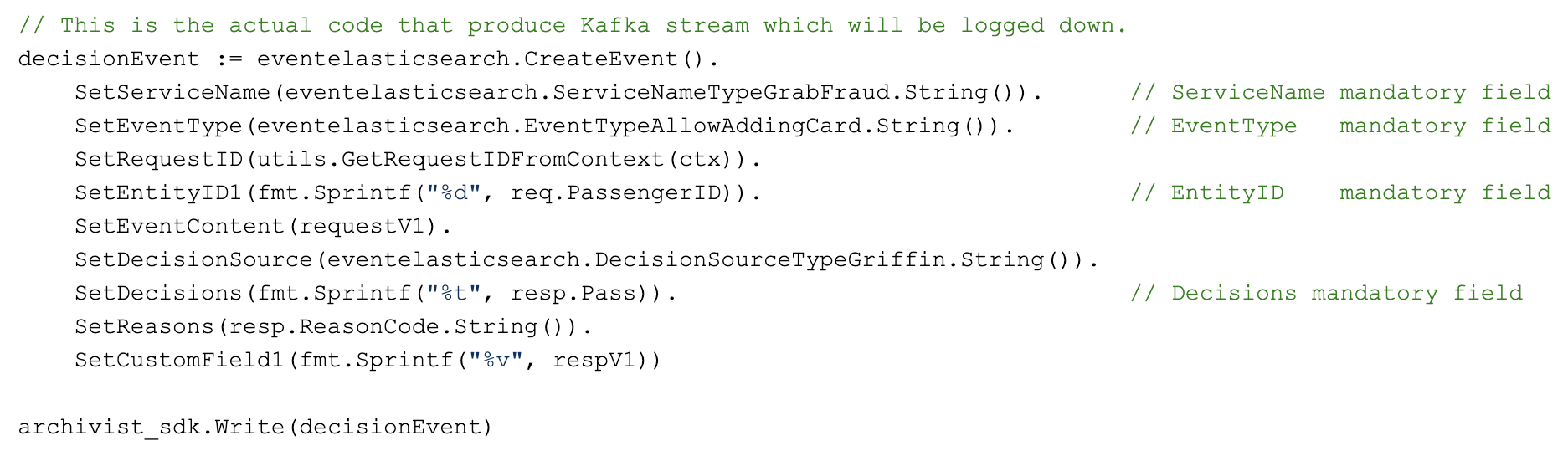
If you want to get onboard Archivist, the coding effort is minimal. Here is an example of a code snippet to log an event:
Code snippet to log an event
Lessons
During the implementation of Archivist, we learnt some things:
A good system needs to support multi-tenants from the beginning. Originally, we thought we could use just one Kafka stream, and put all the documents from different teams into one ElasticSearch (ES) index. But after one team insisted on keeping their data separately from others, we created more Kafka streams and ES indexes. We realised that this way, it’s easier for us to manage data and share the cost fairly.
Shortly after we launched Archivist, there was an incident where the ES data writes were choked. Because each document write is a goroutine, the number of goroutines increased to 400k and the memory usage reached 100% within minutes. We added a patch (2 lines of code) to limit the maximum number of goroutines in our system. Since then, we haven’t had any more severe incidents in Archivist.
Join Us
Grab is the leading superapp platform in Southeast Asia, providing everyday services that matter to consumers. More than just a ride-hailing and food delivery app, Grab offers a wide range of on-demand services in the region, including mobility, food, package and grocery delivery services, mobile payments, and financial services across 428 cities in eight countries.
Powered by technology and driven by heart, our mission is to drive Southeast Asia forward by creating economic empowerment for everyone. If this mission speaks to you, join our team today!
The collective thoughts of the interwebz
Manage Consent
To provide the best experiences, we use technologies like cookies to store and/or access device information. Consenting to these technologies will allow us to process data such as browsing behavior or unique IDs on this site. Not consenting or withdrawing consent, may adversely affect certain features and functions.
Functional
Always active
The technical storage or access is strictly necessary for the legitimate purpose of enabling the use of a specific service explicitly requested by the subscriber or user, or for the sole purpose of carrying out the transmission of a communication over an electronic communications network.
Preferences
The technical storage or access is necessary for the legitimate purpose of storing preferences that are not requested by the subscriber or user.
Statistics
The technical storage or access that is used exclusively for statistical purposes.The technical storage or access that is used exclusively for anonymous statistical purposes. Without a subpoena, voluntary compliance on the part of your Internet Service Provider, or additional records from a third party, information stored or retrieved for this purpose alone cannot usually be used to identify you.
Marketing
The technical storage or access is required to create user profiles to send advertising, or to track the user on a website or across several websites for similar marketing purposes.