Post Syndicated from BP Yau original https://aws.amazon.com/blogs/big-data/unlocking-near-real-time-analytics-with-petabytes-of-transaction-data-using-amazon-aurora-zero-etl-integration-with-amazon-redshift-and-dbt-cloud/
While customers can perform some basic analysis within their operational or transactional databases, many still need to build custom data pipelines that use batch or streaming jobs to extract, transform, and load (ETL) data into their data warehouse for more comprehensive analysis.
Zero-ETL integration with Amazon Redshift reduces the need for custom pipelines, preserves resources for your transactional systems, and gives you access to powerful analytics. Within seconds of transactional data being written into Amazon Aurora (a fully managed modern relational database service offering performance and high availability at scale), the data is seamlessly made available in Amazon Redshift for analytics and machine learning. The data in Amazon Redshift is transactionally consistent and updates are automatically and continuously propagated.
Amazon Redshift is a fast, scalable, secure, and fully managed cloud data warehouse that makes it simple and cost-effective to analyze all your data using standard SQL and your existing ETL, business intelligence (BI), and reporting tools. Together with price-performance, Amazon Redshift offers capabilities such as serverless architecture, machine learning integration within your data warehouse and secure data sharing across the organization.
dbt helps manage data transformation by enabling teams to deploy analytics code following software engineering best practices such as modularity, continuous integration and continuous deployment (CI/CD), and embedded documentation.
dbt Cloud is a hosted service that helps data teams productionize dbt deployments. dbt Cloud offers turnkey support for job scheduling, CI/CD integrations; serving documentation, native git integrations, monitoring and alerting, and an integrated developer environment (IDE) all within a web-based UI.
In this post, we explore how to use Aurora MySQL-Compatible Edition Zero-ETL integration with Amazon Redshift and dbt Cloud to enable near real-time analytics. By using dbt Cloud for data transformation, data teams can focus on writing business rules to drive insights from their transaction data to respond effectively to critical, time sensitive events. This enables the line of business (LOB) to better understand their core business drivers so they can maximize sales, reduce costs, and further grow and optimize their business.
Solution overview
Let’s consider TICKIT, a fictional website where users buy and sell tickets online for sporting events, shows, and concerts. The transactional data from this website is loaded into an Aurora MySQL 3.05.0 (or a later version) database. The company’s business analysts want to generate metrics to identify ticket movement over time, success rates for sellers, and the best-selling events, venues, and seasons. Analysts can use this information to provide incentives to buyers and sellers who frequently use the site, to attract new users, and to drive advertising and promotions.
The Zero-ETL integration between Aurora MySQL and Amazon Redshift is set up by using a CloudFormation template to replicate raw ticket sales information to a Redshift data warehouse. After the data is in Amazon Redshift, dbt models are used to transform the raw data into key metrics such as ticket trends, seller performance, and event popularity. These insights help analysts make data-driven decisions to improve promotions and user engagement.
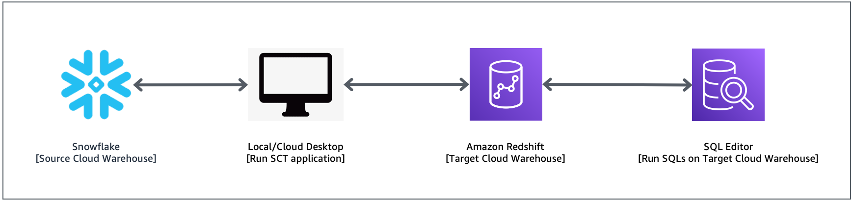
The following diagram illustrates the solution architecture at a high-level.

To implement this solution, complete the following steps:
- Set up Zero-ETL integration from the AWS Management Console for Amazon Relational Database Service (Amazon RDS).
- Create dbt models in dbt Cloud.
- Deploy dbt models to Amazon Redshift.
Prerequisites
- A dbt Cloud account. Sign up for one if you haven’t already done so.
- An AWS Identity and Access Management (IAM) user with sufficient permissions to interact with the AWS Management Console and related AWS services. Your IAM permissions must also include access to create IAM roles and policies through the AWS CloudFormation template.
Set up resources with CloudFormation
This post provides a CloudFormation template as a general guide. You can review and customize it to suit your needs. Some of the resources that this stack deploys incur costs when in use.
The CloudFormation template provisions the following components
- An Aurora MySQL provisioned cluster (source)
- An Amazon Redshift Serverless data warehouse (target)
- Zero-ETL integration between the source (Aurora MySQL) and target (Amazon Redshift Serverless)
To create your resources:
- Sign in to the console.
- Choose the us-east-1 AWS Region in which to create the stack.
- Choose Launch Stack
![]()
- Choose Next.
This automatically launches CloudFormation in your AWS account with a template. It prompts you to sign in as needed. You can view the CloudFormation template from within the console.
- For Stack name, enter a stack name.
- Keep the default values for the rest of the Parameters and choose Next.
- On the next screen, choose Next.
- Review the details on the final screen and select I acknowledge that AWS CloudFormation might create IAM resources.
- Choose Submit.
Stack creation can take up to 30 minutes.
- After the stack creation is complete go to the Outputs tab of the stack and record the values of the keys for the following components, which you will use in a later step:
NamespaceNamePortNumberRDSPasswordRDSUsernameRedshiftClusterSecurityGroupNameRedshiftPasswordRedshiftUsernameVPCWorkinggroupnameZeroETLServicesRoleNameArn

- Configure your Amazon Redshift data warehouse security group settings to allow inbound traffic from dbt IP addresses.
- You’re now ready to sign in to both Aurora MySQL cluster and Amazon Redshift Serverless data warehouse and run some basic commands to test them.
Create a database from integration in Amazon Redshift
To create a target database using Redshift query editor V2:
- On the Amazon Redshift Serverless console, choose the zero-etl-destination workgroup.
- Choose Query data to open Query Editor v2.
- Connect to an Amazon Redshift Serverless data warehouse using the username and password from the CloudFormation resource creation step.
- Get the
integration_idfrom thesvv_integrationsystem table.
- Use the
integration_idfrom the preceding step to create a new database from the integration.
The integration between Aurora MYSQL and the Amazon Redshift Serverless data warehouse is now complete.
Populate source data in Aurora MySQL
You’re now ready to populate source data in Amazon Aurora MYSQL.
You can use your favorite query editor installed on either an Amazon Elastic Compute Cloud (Amazon EC2) instance or your local system to interact with Aurora MYSQL. However, you need to provide access to Aurora MYSQL from the machine where the query editor is installed. To achieve this, modify the security group inbound rules to allow the IP address of your machine and make Aurora publicly accessible.
To populate source data:
- Run the following script on Query Editor to create the sample database DEMO_DB and tables inside DEMO_DB.
- Load data from Amazon Simple Storage Service (Amazon S3) to the corresponding table using the following commands:
The following are common errors associated with load from Amazon S3:
- For the current version of the Aurora MySQL cluster, set the
aws_default_s3_roleparameter in the database cluster parameter group to the role Amazon Resource Name (ARN) that has the necessary Amazon S3 access permissions. - If you get an error for missing credentials, such as the following, you probably haven’t associated your IAM role to the cluster. In this case, add the intended IAM role to the source Aurora MySQL cluster.
Error 63985 (HY000): S3 API returned error: Missing Credentials: Cannot instantiate S3 Client),
Validate the source data in your Amazon Redshift data warehouse
To validate the source data
- Navigate to the Redshift Serverless dashboard, open Query Editor v2, and select the workgroup and database created from integration from the drop-down list. Expand the database
aurora_zeroetl, schemademodband you should see 7 tables being created. - Wait a few seconds and run the following SQL query to see integration in action.
Transforming data with dbtCloud
Connect dbt Cloud to Amazon Redshift
- Create a new project in dbt Cloud. From Account settings (using the gear menu in the top right corner), choose + New Project.
- Enter a project name and choose Continue.

- For Connection, select Add new connection from the drop-down list.
- Select Redshift and enter the following information:
- Connection name: The Name of the connection.
- Server Hostname: Your Amazon Redshift Serverless endpoint.
- Port:
Redshift 5439. - Database name:
dev.
- Make sure you allowlist your dbt Cloud IP address in your Redshift data warehouse security group inbound traffic.
- Choose Save to set up your connection.

- Set your development credentials. These credentials will be used by dbt Cloud to connect to your Amazon Redshift data warehouse. See the CloudFormation template output for the credentials.
- Schema –
dbt_zetl. dbt Cloud automatically generates a schema name for you. By convention, this isdbt_<first-initial><last-name>. This is the schema connected directly to your development environment, and it’s where your models will be built when running dbt within the Cloud integrated development environment (IDE).

- Choose Test Connection. This verifies that dbt Cloud can access your Redshift data warehouse.
- Choose Next if the test succeeded. If it failed, check your Amazon Redshift settings and credentials.
Set up a dbt Cloud managed repository
When you develop in dbt Cloud, you can use git to version control your code. For the purposes of this post, use a dbt Cloud-hosted managed repository.
To set up a managed repository:
- Under Setup a repository, select Managed.
- Enter a name for your repo, such as
dbt-zeroetl. - Choose Create. It will take a few seconds for your repository to be created and imported.

Initialize your dbt project and start developing
Now that you have a repository configured, initialize your project and start developing in dbt Cloud.
To start development in dbt Cloud:
- In dbt Cloud, choose Start developing in the IDE. It might take a few minutes for your project to spin up for the first time as it establishes your git connection, clones your repo, and tests the connection to the warehouse.

- Above the file tree to the left, choose Initialize dbt project. This builds out your folder structure with example models.

- Make your initial commit by choosing Commit and sync. Use the commit message initial commit and choose Commit Changes. This creates the first commit to your managed repo and allows you to open a branch where you can add new dbt code.

To build your models
- Under Version Control on the left, choose Create branch. Enter a name, such as
add-redshift-models. You need to create a new branch because the main branch is set to read-only mode. - Choose
dbt_project.yml. - Update the models section of
dbt_project.ymlat the bottom of the file. Change example to staging and make sure the materialized value is set to table.
models:
my_new_project:
# Applies to all files under models/example/
staging:
materialized: table
- Choose the three-dot icon (…) next to the models directory, then select Create Folder.
- Name the folder staging, then choose Create.
- Choose the three-dot icon (…) next to the models directory, then select Create Folder.
- Name the folder
dept_finance, then choose Create. - Choose the three-dot icon (…) next to the staging directory, then select Create File.

- Name the file
sources.yml, then choose Create. - Copy the following query into the file and choose Save.
Be aware that the operation database created on your Amazon Redshift data warehouse is a special read only database and you cannot directly connect to it to create objects. You need to connect to another regular database and use three-part notation as defined in sources.yml to query data from it.
- Choose the three-dot icon (…) directory, then select Create File.
- Name the file
staging_event.sql, then choose Create. - Copy the following query into the file and choose Save.
- Choose the three-dot icon (…) next to the staging directory, then select Create File.
- Name the file
staging_sales.sql, then choose Create. - Copy the following query into the file and choose Save.
- Choose the three-dot icon (…) next to the dept_finance directory, then select Create File.
- Name the file
rpt_finance_qtr_total_sales_by_event.sql, then choose Create. - Copy the following query into the file and choose Save.
- Choose the three-dot icon (…) next to the dept_finance directory, then select Create File.
- Name the file
rpt_finance_qtr_top_event_by_sales.sql, then choose Create. - Copy the following query into the file and choose Save.
- Choose the three-dot icon (…) next to the example directory, then select Delete.
- Enter dbt run in the command prompt at the bottom of the screen and press Enter.

- You should get a successful run and see the four models.

- Now that you have successfully run the dbt model, you should be able to find it in the Amazon Redshift data warehouse. Go to Redshift Query Editor v2, refresh the dev database, and verify that you have a new
dbt_zetlschema with thestaging_eventandstaging_salestables andrpt_finance_qtr_top_event_by_salesandrpt_finance_qtr_total_sales_by_eventviews in it.

- Run the following SQL statement to verify that data has been loaded into your Amazon Redshift table.
Add tests to your models
Adding tests to a project helps validate that your models are working correctly.
To add tests to your project:
- Create a new YAML file in the models directory and name it
models/schema.yml. - Add the following contents to the file:
- Run dbt test, and confirm that all your tests passed.
- When you run
dbt test, dbt iterates through your YAML files and constructs a query for each test. Each query will return the number of records that fail the test. If this number is 0, then the test is successful.
Document your models
By adding documentation to your project, you can describe your models in detail and share that information with your team.
To add documentation:
- Run dbt docs generate to generate the documentation for your project. dbt inspects your project and your warehouse to generate a JSON file documenting your project.

- Choose the book icon in the Develop interface to launch documentation in a new tab.


Commit your changes
Now that you’ve built your models, you need to commit the changes you made to the project so that the repository has your latest code.
To commit the changes:
- Under Version Control on the left, choose Commit and sync and add a message. For example,
Add Aurora zero-ETL integration with Redshift models.

- Choose Merge this branch to main to add these changes to the main branch on your repo.
Deploy dbt
Use dbt Cloud’s Scheduler to deploy your production jobs confidently and build observability into your processes. You’ll learn to create a deployment environment and run a job in the following steps.
To create a deployment environment:
- In the left pane, select Deploy, then choose Environments.

- Choose Create Environment.
- In the Name field, enter the name of your deployment environment. For example,
Production. - In the dbt Version field, select Versionless from the dropdown.
- In the Connection field, select the connection used earlier in development.
- Under Deployment Credentials, enter the credentials used to connect to your Redshift data warehouse. Choose Test Connection.

- Choose Save.
Create and run a job
Jobs are a set of dbt commands that you want to run on a schedule.
To create and run a job:
- After creating your deployment environment, you should be directed to the page for a new environment. If not, select Deploy in the left pane, then choose Jobs.
- Choose Create job and select Deploy job.
- Enter a Job name, such as,
Production run, and link to the environment you just created. - Under Execution Settings, select Generate docs on run.
- Under Commands, add this command as part of your job if you don’t see them:
dbt build
- For this exercise, don’t set a schedule for your project to run—while your organization’s project should run regularly, there’s no need to run this example project on a schedule. Scheduling a job is sometimes referred to as deploying a project.

- Choose Save, then choose Run now to run your job.
- Choose the run and watch its progress under Run history.
- After the run is complete, choose View Documentation to see the docs for your project.
Clean up
When you’re finished, delete the CloudFormation stack since some of the AWS resources in this walkthrough incur a cost if you continue to use them. Complete the following steps:
- On the CloudFormation console, choose Stacks.
- Choose the stack you launched in this walkthrough. The stack must be currently running.
- In the stack details pane, choose Delete.
- Choose Delete stack.
Summary
In this post, we showed you how to set up Amazon Aurora MySQL Zero-ETL integration from Aurora MySQL to Amazon Redshift, which eliminates complex data pipelines and enables near real-time analytics on transactional and operational data. We also showed you how to build dbt models on Aurora MySQL Zero-ETL integration tables in Amazon Redshift to transform the data to get insight.
We look forward to hearing from you about your experience. If you have questions or suggestions, leave a comment.
About the authors
 BP Yau is a Sr Partner Solutions Architect at AWS. His role is to help customers architect big data solutions to process data at scale. Before AWS, he helped Amazon.com Supply Chain Optimization Technologies migrate its Oracle data warehouse to Amazon Redshift and build its next generation big data analytics platform using AWS technologies.
 Saman Irfan is a Senior Specialist Solutions Architect at Amazon Web Services, based in Berlin, Germany. She collaborates with customers across industries to design and implement scalable, high-performance analytics solutions using cloud technologies. Saman is passionate about helping organizations modernize their data architectures and unlock the full potential of their data to drive innovation and business transformation. Outside of work, she enjoys spending time with her family, watching TV series, and staying updated with the latest advancements in technology.
 Raghu Kuppala is an Analytics Specialist Solutions Architect experienced working in the databases, data warehousing, and analytics space. Outside of work, he enjoys trying different cuisines and spending time with his family and friends.
 Neela Kulkarni is a Solutions Architect with Amazon Web Services. She primarily serves independent software vendors in the Northeast US, providing architectural guidance and best practice recommendations for new and existing workloads. Outside of work, she enjoys traveling, swimming, and spending time with her family.


 Srikanth Sopirala is a Sr. Specialist Solutions Architect, Analytics at AWS. He is passionate about helping customers build scalable data and analytics solutions in the cloud.
 Zhouyi Yang is a Software Development Engineer for Amazon Redshift Query Processing team. He’s passionate about gaining new knowledge about large databases and has worked on SQL language features such as federated query and IAM role privilege control. In his spare time, he enjoys swimming, tennis, and reading.
 Entong Shen is a Senior Software Development Engineer for Amazon Redshift. He has been working on MPP databases for over 8 years and has focused on query optimization, statistics, and SQL language features such as stored procedures and federated query. In his spare time, he enjoys listening to music of all genres and working in his succulent garden.