Post Syndicated from Donatas Kuchalskis original https://aws.amazon.com/blogs/big-data/build-a-multi-region-analytics-solution-with-amazon-redshift-amazon-s3-and-amazon-quicksight/
Organizations increasingly face complex requirements balancing regional data sovereignty with global analytics needs. Regulatory frameworks like GDPR, HIPAA, and local data protection laws often mandate storing data in specific geographic regions, and business operations require global teams to access and analyze this data efficiently.
This post explores how to effectively architect a solution that addresses this specific challenge: enabling comprehensive analytics capabilities for global teams while making sure that your data remains in the AWS Regions required by your compliance framework. We use a variety of AWS services, including Amazon Redshift, Amazon Simple Storage Service (Amazon S3), and Amazon QuickSight.
It’s important to note that this solution focuses primarily on data residency (where data is stored) and not on preventing data from being in transit between Regions. Organizations with strict data transit restrictions might need additional controls beyond what’s covered here. We show how you can configure AWS across Regions to help meet business needs and regulatory requirements simultaneously.
Cross-Region architecture requirements
Before implementing a cross-Region solution, it’s important to understand when this approach is actually necessary. Although single-Region deployments offer simplicity and cost advantages, several specific business and regulatory scenarios warrant a cross-Region approach:
- Data sovereignty and residency requirements – When regulations like GDPR, HIPAA, or local data sovereignty laws require data to remain in specific geographic boundaries while still enabling global analytics capabilities
- Global operations with local compliance – When your organization operates globally, but needs to adhere to regional compliance frameworks while maintaining unified analytics
- Performance optimization for global users – When your organization needs to optimize analytics performance for users in different geographic areas while centralizing data governance
- Enhanced business continuity – When your analytics capabilities need higher availability and Regional redundancy to support mission-critical business processes
Use case: Financial services analytics with Regional data residency
Consider a financial services company with the following business and regulatory requirements:
- Data residency requirement – All customer financial data must remain in the Bahrain Region (me-south-1) to comply with local financial regulations.
- Global analytics capability – The organization’s data science team operates from European offices and needs to access and analyze the financial data without moving it out of its mandated storage Region.
- Advanced analytics requirements – Business leaders need interactive data exploration and natural language query capabilities to derive insights from financial data.
- Performance requirement – Specific dashboard queries require subsecond response times for both local executives and the global management team.
This specific combination of requirements can’t be met with a single-Region deployment. Let’s explore how to architect a solution.
Solution overview
The following architecture is designed to address the specific challenge of using QuickSight in one Region while maintaining data in another Region.

As shown in the architecture diagram, data engineers based in Bahrain (me-south-1) work with local data, whereas data engineers in Stockholm (eu-north-1) and analysts in Ireland (eu-west-1) can securely access the same data through Redshift datashares and virtual private cloud (VPC) peering connections. This approach maintains data residency in me-south-1 while enabling global access.
The solution consists of the following key components:
- Primary data Region (me-south-1):
- Redshift cluster (primary data repository)
- S3 buckets for data lake storage
- Private and public subnets with appropriate security controls
- Data must remain in this Region for compliance reasons
- Analytics services Region (eu-west-1):
- QuickSight deployment
- Cross-Region VPC peering connection to the primary Region
- Data access using Redshift datashares (no data replication)
- Data engineering Region (eu-north-1):
- Redshift consumer cluster for data engineering workloads
- Data access using Redshift datashares from me-south-1
- Makes it possible for data engineering teams in eu-north-1 to access and work with data while maintaining compliance
Before implementing this architecture, evaluate whether:
- Your requirements actually necessitate a cross-Region approach
- The performance impact is acceptable for your use case
- The additional cost is justified by your business requirements
For most analytics workloads, a single-Region architecture remains the recommended approach for simplicity, performance, and cost-effectiveness. Consider cross-Region architectures only when specific business and compliance requirements make them necessary.
Establish cross-Region network connectivity: Amazon Redshift to QuickSight
The foundation of a cross-Region solution is secure, reliable network connectivity. VPC peering provides a straightforward approach for connecting VPCs across Regions. To implement VPC peering in Amazon Virtual Private Cloud (Amazon VPC), complete the following steps:
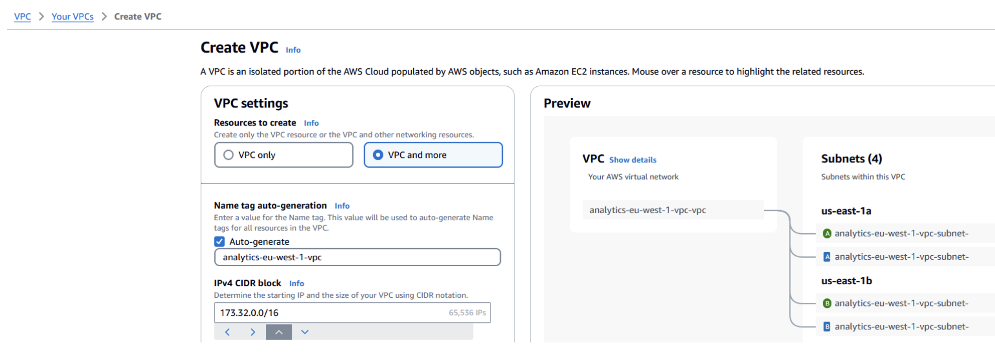
- Create a new VPC in the secondary Region (eu-west-1):
- Open the Amazon VPC console in the eu-west-1 Region.
- Choose Create VPC.
- Set IPv4 CIDR block to 172.32.0.0/16 (verify there is no overlap with the primary Region VPC).
- Select Auto-generate to create subnets automatically within this new VPC.
- Leave other settings as default and choose Create VPC.
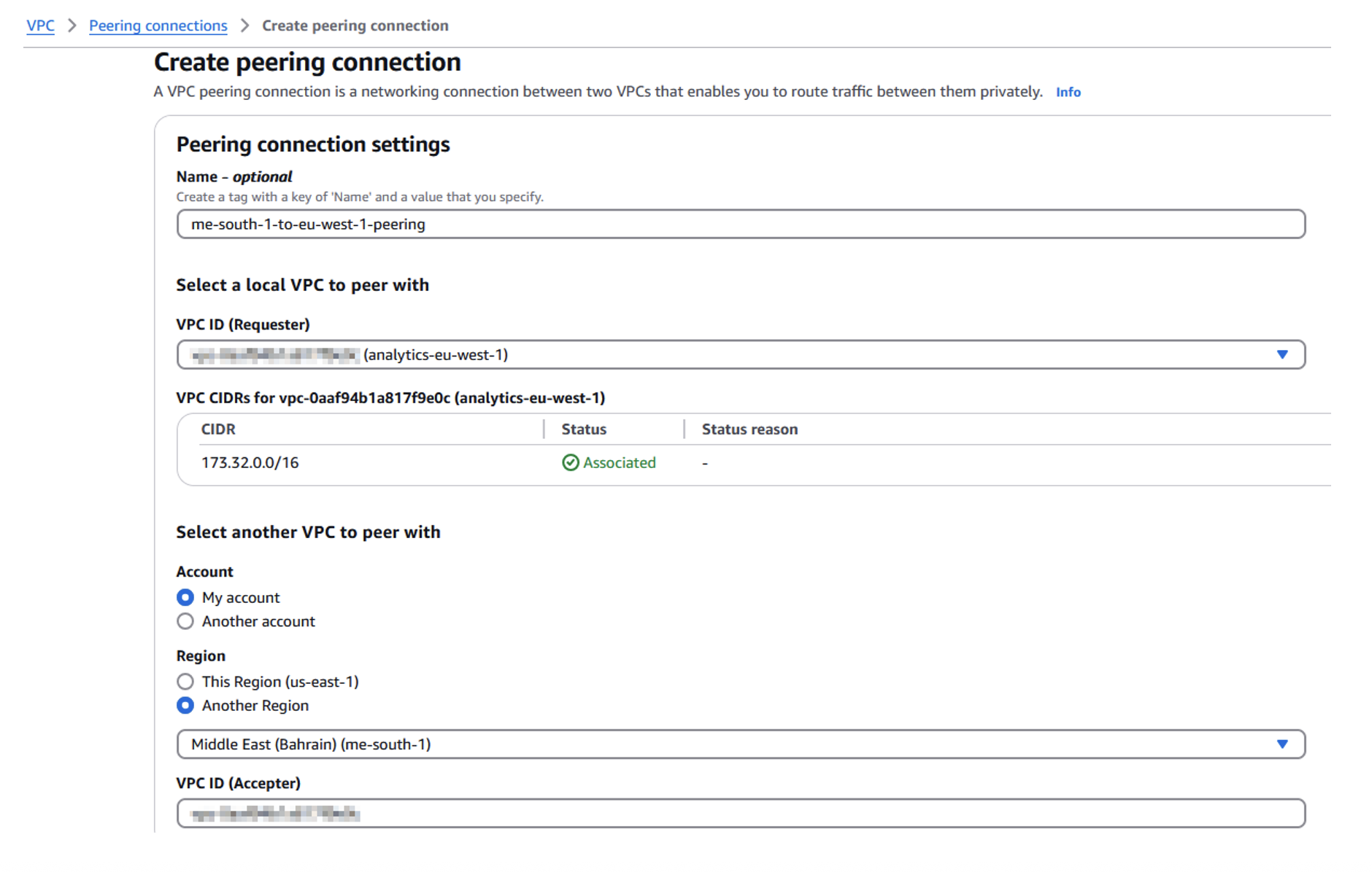
- Set up VPC peering:
- On the Amazon VPC console, choose Peering connections in the navigation pane and choose Create peering connection.
- Select the new eu-west-1 VPC as the requester.
- For Select another VPC to peer with, select My account and Another Region.
- Choose the primary Region (me-south-1) and enter the VPC ID.
- Choose Create peering connection.
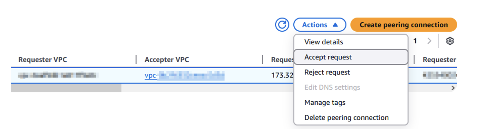
- Accept the VPC peering connection:
- Switch to the primary Region on the Amazon VPC console.
- Choose Peering connections in the navigation pane and select the pending connection.
- On the Actions dropdown menu, choose Accept request.
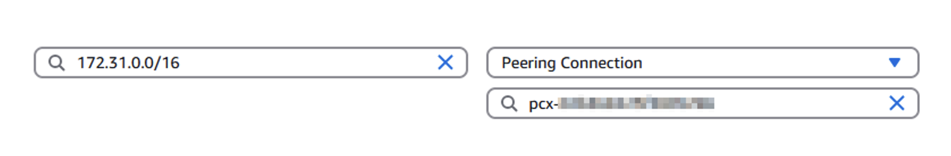
- Update the route tables:
- On the secondary Region Amazon VPC console, choose Route tables in the navigation pane.
- Choose the route table for the new VPC.
- Choose Edit routes and add a new route:
- Destination: Primary Region VPC CIDR (e.g., 172.31.0.0/16).
- Target: Choose the peering connection.
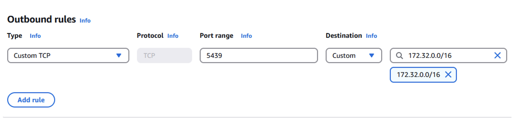
- On the primary Region Amazon VPC console, repeat the process, adding a route to the secondary Region VPC CIDR (172.32.0.0/16) using the peering connection.
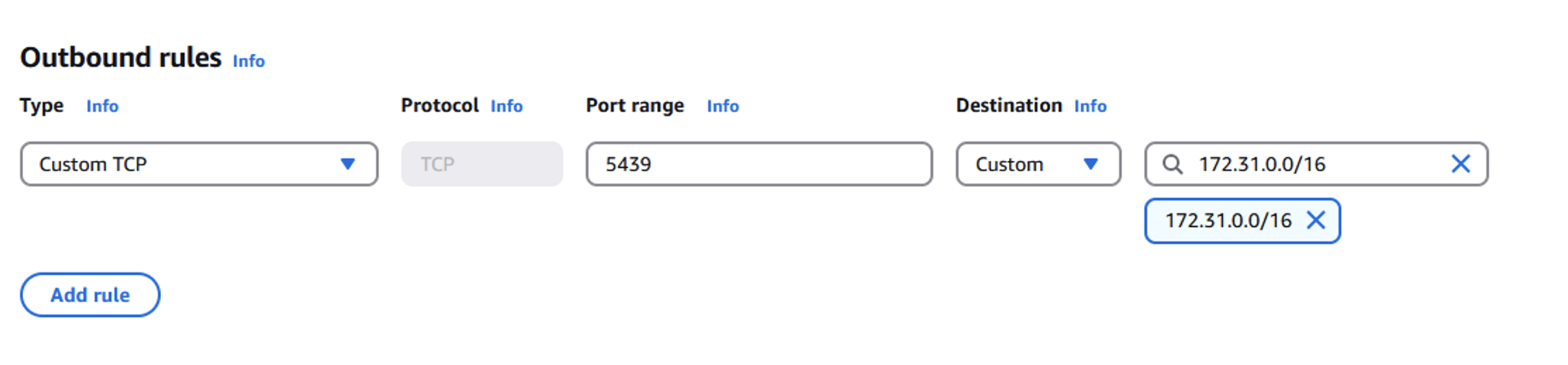
- Configure security groups:
- On the secondary Region Amazon VPC console, choose Security groups in the navigation pane and create a new security group.
- Add an outbound rule:
- Type: Custom TCP
- Port range: 5439
- Destination: Primary Region VPC CIDR

- On the primary Region Amazon VPC console, locate the Redshift cluster’s security group.
- Add an inbound rule:
- Type: Custom TCP
- Port range: 5439
- Source: Secondary Region VPC CIDR
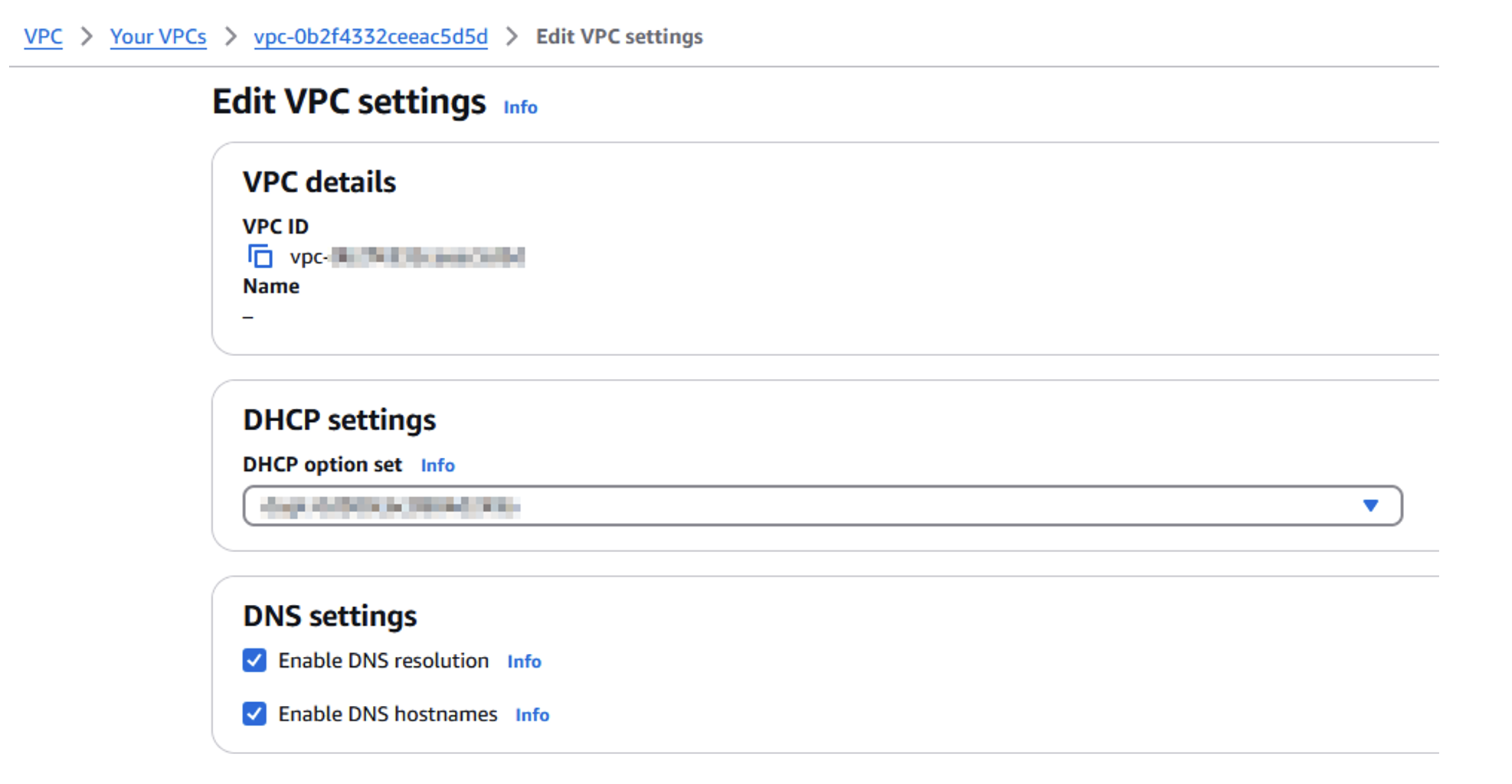
- Configure DNS settings:
- On the Amazon VPC console for both Regions, choose Your VPCs in the navigation pane.
- Select each VPC, and on the Actions dropdown menu, choose Edit DNS hostnames.
- Select Enable DNS resolution and Enable DNS hostnames.
Implement cross-Region data sharing
Rather than replicating data, which could create compliance issues, you can use Redshift datashares to provide secure, read-only access to data across Regions. Complete the following steps to set up your datashares:
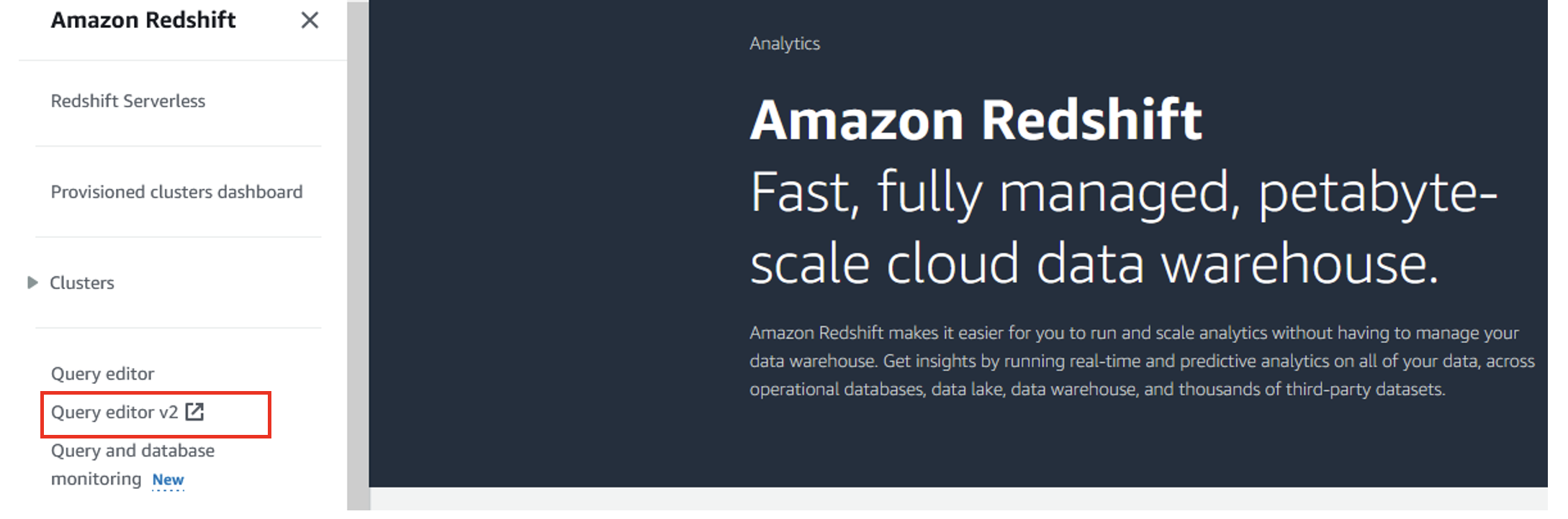
- Create producer datashares in the primary Region:
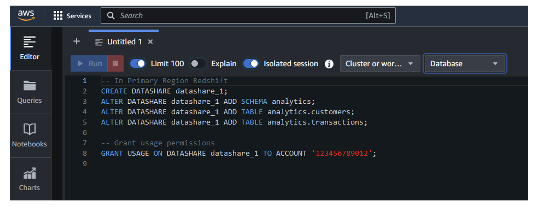
- On the Amazon Redshift console, choose Query editor v2 in the navigation pane to connect to your primary Region Redshift cluster (me-south-1).

- Run the following commands:
-- In Primary Region Redshift

CREATE DATASHARE datashare_1;
ALTER DATASHARE datashare_1 ADD SCHEMA analytics;
ALTER DATASHARE datashare_1 ADD TABLE analytics.customers;
ALTER DATASHARE datashare_1 ADD TABLE analytics.transactions;

-- Grant usage permissions

GRANT USAGE ON DATASHARE datashare_1 TO ACCOUNT '123456789012';
- On the Amazon Redshift console, choose Query editor v2 in the navigation pane to connect to your primary Region Redshift cluster (me-south-1).
- Create a consumer database in the secondary Region:
- Connect to your secondary Region Redshift cluster (eu-west-1) using the query editor and run the following commands:
-- In Secondary Region Redshift CREATE DATABASE consumer_db FROM DATASHARE datashare_1 OF ACCOUNT '123456789012'REGION 'me-south-1'; - Verify the datashare configuration with the following code:
-- In Secondary Region Redshift

SELECT * FROM SVV_DATASHARE_CONSUMERS;
SELECT * FROM SVV_DATASHARE_OBJECTS;
This approach maintains data residency in the primary Region while enabling analytics access from another Region, addressing the core challenge of Regional service limitations. For our financial services company example, this makes sure that customer financial data remains in Bahrain (me-south-1) while making it securely accessible to the data science team in Europe (eu-west-1).
Configure QuickSight in the analytics Region
With network connectivity and data sharing established, complete the following steps to configure QuickSight to securely access the Redshift data:
- Set up a QuickSight VPC connection:
- Open the QuickSight console in the secondary Region.
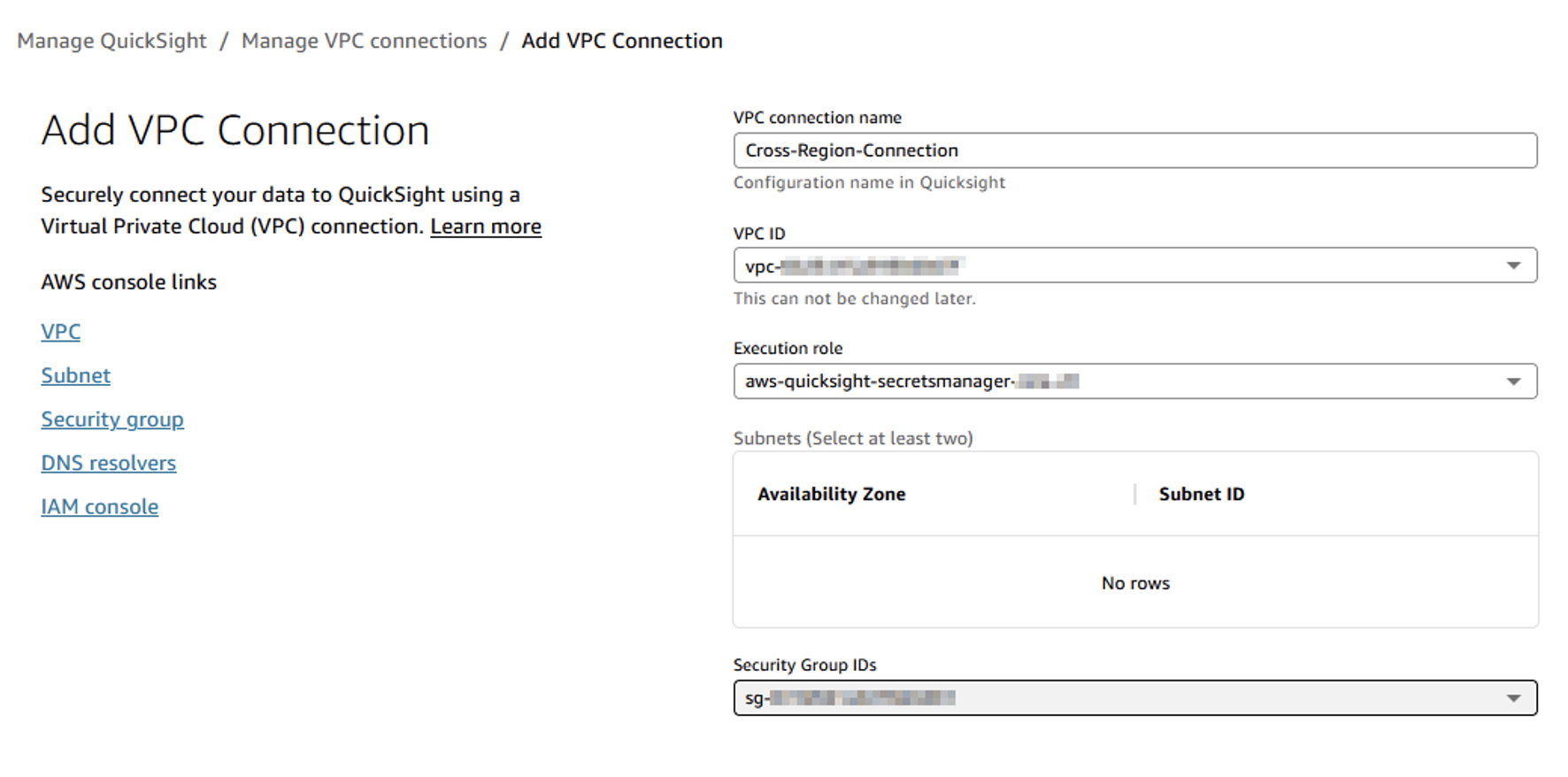
- Choose Manage QuickSight, VPC connections, and Add VPC connection.
- Configure the connection:
- Name: Enter a name (for example, Cross-Region-Connection).
- VPC: Choose the secondary Region VPC.
- Subnet: Choose the automatically created subnets.
- Security group: Choose the security group created for cross-Region access.
- Add a QuickSight IP range to the data source security group:
- Open the Amazon Elastic Compute Cloud (Amazon EC2) console in the primary Region.
- Choose Security groups in the navigation pane and find the security group for your data source.
- Edit the inbound rules.
- Add a new rule:
- Type: HTTPS (443)
- Protocol: TCP
- Port range: 443
- Source: QuickSight IP range for the secondary Region (for example, 52.210.255.224/27 for eu-west-1).
QuickSight IP ranges can change over time. Refer to AWS Regions, websites, IP address ranges, and endpoints for current IP ranges.
- Create a QuickSight data source:
- On the QuickSight console, choose Datasets in the navigation pane.
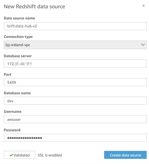
- Choose New dataset, then choose Redshift.
- Configure the connection:
- Data source name: Enter a descriptive name.
- Connection type: Choose the VPC connection.
- Database server: Enter the Redshift cluster endpoint from the primary Region.
- Port: 5439
- Database name: Enter the consumer database name.
- Username and Password: Enter credentials (consider using AWS Secrets Manager).
- Choose Validate connection to test.
- Choose Create data source.
- Verify the connection and create datasets:
- Choose the schema and tables from the consumer database.
- Configure appropriate refresh schedules.
- Create calculations and visualizations as needed.
Performance considerations for cross-Region analytics
When implementing a cross-Region analytics architecture, be aware of the following performance implications:
- Query performance impact – Cross-Region queries can experience higher latency than single-Region queries. To mitigate this, consider the following:
- Use SPICE for QuickSight – Import frequently-used datasets into SPICE (Super-fast, Parallel, In-memory Calculation Engine) to help avoid repeated cross-Region queries. SPICE is the QuickSight in-memory engine that enables fast, interactive visualizations by precomputing and storing datasets locally in the QuickSight Region.
- Implement efficient query patterns – Minimize the amount of data transferred between Regions.
- Use appropriate caching – Enable result caching where possible.
- Monitoring cross-Region performance – Implement monitoring to identify and address performance issues:
- Set up Amazon CloudWatch metrics to track cross-Region query performance
- Create dashboards to visualize latency trends
- Establish performance baselines and alerts for degradation
Security considerations
Maintaining security in a cross-Region architecture requires additional attention:
- Network security:
- Limit VPC peering connections to only necessary VPCs
- Implement restrictive security groups that allow only required traffic
- Consider using VPC endpoints for service access when possible
- Data access controls:
- Use AWS Identity and Access Management (IAM) policies consistently across Regions
- Implement fine-grained access controls in Redshift datashares
- Enable audit logging in relevant Regions
- Compliance monitoring:
- Implement AWS CloudTrail in all Regions
- Create centralized logging for cross-Region activities
- Regularly review cross-Region access patterns
Cost implications
Before implementing a cross-Region architecture, consider these cost factors:
- Data transfer costs – Data transfer between Regions incurs charges
- Additional infrastructure – You might need Redshift clusters in multiple Regions
- VPC peering costs – Data transfer costs are associated with VPC peering
- Operational overhead – Managing multi-Region deployments requires additional resources
- Workload-based sizing – You should size each Regional Redshift cluster according to the specific workloads it will handle
Conclusion
The cross-Region architecture described in this post addresses specific challenges related to Regional compliance requirements and global analytics needs, particularly in the following scenarios:
- Your data must remain in a specific Region for compliance reasons
- You have teams in different Regions who need to access and analyze this data
- Different user groups have distinct workload requirements
The datasharing capabilities of Amazon Redshift and Regional storage options in Amazon S3 are key enablers of this solution, allowing data to remain in the required Region while still being accessible for analytics across Regions. However, it’s worth emphasizing that this architecture supports data storage in specific Regions but doesn’t prevent data from traveling between Regions during processing. Organizations concerned about data transit restrictions should evaluate additional controls to address those specific requirements. Combined with secure VPC peering connections and QuickSight visualizations, this architecture creates a complete solution that satisfies both compliance requirements and business needs.
For our financial services example, this architecture successfully enables the company to keep its customer financial data in Bahrain while providing seamless analytics capabilities to the European data science team and delivering interactive dashboards to global business leaders.
For more information, refer to Building a Cloud Security Posture Dashboard with Amazon QuickSight. For hands-on experience, explore the Amazon QuickSight Workshops. Visit the Amazon Redshift console or Amazon QuickSight console to start building your first dashboard, and explore our AWS Big Data Blog for more customer success stories and implementation patterns
Try out this solution for your own use case, and share your thoughts in the comments.
About the Authors
 Donatas Kuchalskis is a Cloud Operations Architect at AWS, based in London, focusing on Financial Services customers in the UK. He helps customers optimize their AWS environments for cost, security, and resiliency while providing strategic cloud guidance. Prior to this role, he served as a Prototyping Architect specializing in Big Data and as a Specialist Solutions Architect for Retail. Before joining AWS, Donatas spent 6 years as a technical consultant in the retail sector.
 Jumana Nagaria is a Prototyping Architect at AWS. She builds innovative prototypes with customers to solve their business challenges. She is passionate about cloud computing and data analytics. Outside of work, Jumana enjoys travelling, reading, painting, and spending quality time with friends and family.


 Asser Moustafa is a Principal Worldwide Specialist Solutions Architect at AWS, based in Dallas, Texas, USA. He partners with customers worldwide, advising them on all aspects of their data architectures, migrations, and strategic data visions to help organizations adopt cloud-based solutions, maximize the value of their data assets, modernize legacy infrastructures, and implement cutting-edge capabilities like machine learning and advanced analytics. Prior to joining AWS, Asser held various data and analytics leadership roles, completing an MBA from New York University and an MS in Computer Science from Columbia University in New York. He is passionate about empowering organizations to become truly data-driven and unlock the transformative potential of their data.
 Pinar Yasar is the Data Engineering Manager at Getir. Her passion is to accelerate self-service analytics for her internal customers and build highly scalable and cost-effective solutions in the cloud.


 Chao Pan is a Data Analytics Solutions Architect at Amazon Web Services. He’s responsible for the consultation and design of customers’ big data solution architectures. He has extensive experience in open-source big data. Outside of work, he enjoys hiking.