All posts by Danilo Poccia

New for AWS Lambda – 1ms Billing Granularity Adds Cost Savings

Post Syndicated from Danilo Poccia original https://aws.amazon.com/blogs/aws/new-for-aws-lambda-1ms-billing-granularity-adds-cost-savings/

What I like about AWS Lambda is that it lets you run code without provisioning or managing servers, and you pay only for what you use. Since we launched Lambda in 2014, you have been charged for the number of times your code is triggered (requests) and for the time your code executes, rounded up to the nearest 100ms (duration).

Starting today, we are rounding up duration to the nearest millisecond with no minimum execution time.

With this new pricing, you are going to pay less most of the time, but it’s going to be more noticeable when you have functions whose execution time is much lower than 100ms, such as low latency APIs.

For example, let’s look at a simple web app that I have running. In the Amazon CloudWatch Logs, for each invocation there is a REPORT line. To improve readability, I am breaking the REPORT line into three lines here:

REPORT RequestId: 35a7e0cb-4902-490d-b8d3-eb315dded660
Duration: 27.40 ms  Billed Duration: 100 ms Memory Size: 1024 MB  Max Memory Used: 472 MB

With 1ms billing granularity that becomes:

REPORT RequestId: a24d03b5-429d-4ca3-a490-878a52a0182f
Duration: 27.55 ms  Billed Duration: 28 ms Memory Size: 1024 MB  Max Memory Used: 472 MB

My application doesn’t have a lot of traffic, so let’s do a simple production scenario. Let’s say I have 100,000 users for a web/mobile app. I expect each user to call this function via the web/mobile app about 20 times per day. The duration of those invocations is on average 28ms. Each month, I should expect:

  • 100,000 users * 20 invocations * 30 days = 60 million invocations.

Let’s estimate the costs in US East (N. Virginia). For simplicity, I am not considering the Lambda free tier.

The Lambda monthly request charges are unchanged:

  • 60 million invocations * $0.20 per 1M requests = $12

To that, I have to add compute charges based on duration.

The Lambda monthly compute charges with the old 100ms rounded up pricing would have been:

  • 60 million invocations* 100ms * 1G memory * $0.0000166667 for every GB-second = $100

With the new 1ms billing granularity, the duration costs are:

  • 60 million invocations * 28ms * 1G memory * $0.0000166667 for every GB-second = $28

For this scenario, overall costs including request and compute charges are much cheaper ($40) than before ($112).

With this pricing, there is now more of an incentive to optimize the duration of functions even if it is already well below 100ms. Your engineering efforts can reduce costs even more.

If you increase memory to get more CPU power and speed up your functions, you now get the benefit of a lower billed duration below 100ms as well. That means that increasing performance and reducing latency is going to be cheaper than before.

We are applying 1ms billing granularity for duration, including when you have Provisioned Concurrency enabled, in all AWS Regions with the exception of those based in China starting with the December 2020 billing period. Regions in China will get the change from January.

Enjoy the new pricing!

Danilo

Coming Soon – EC2 C6gn Instances – 100 Gbps Networking with AWS Graviton2 Processors

Post Syndicated from Danilo Poccia original https://aws.amazon.com/blogs/aws/coming-soon-ec2-c6gn-instances-100-gbps-networking-with-aws-graviton2-processors/

Based on the amazing feedback from customers such as Snap, NextRoll, Intuit, SmugMug, and Honeycomb who are running their workloads on Amazon Elastic Compute Cloud (EC2) instances powered by AWS Graviton2, today we are announcing an addition to our broad Arm-based Graviton2 portfolio with C6gn instances that deliver up to 100 Gbps network bandwidth, up to 38 Gbps Amazon Elastic Block Store (EBS) bandwidth, up to 40% higher packet processing performance, and up to 40% better price/performance versus comparable current generation x86-based network optimized instances.

Compared to C6g instances, this new instance type provides 4x higher network bandwidth, 4x higher packet processing performance, and 2x higher EBS bandwidth. This means that customers with workloads that need high networking bandwidth such as high performance computing (HPC), network appliance, real-time video communications, and data analytics, will be able to bring their biggest and most challenging applications to Arm and take advantage of the performance and cost-optimization.

C6gn instances will be available in 8 sizes:

Name vCPUs Memory
(GiB)
Network Bandwidth
(Gbps)
EBS Throughput
(Gbps)
c6gn.medium 1 2 Up to 25 Up to 9.5
c6gn.large 2 4 Up to 25 Up to 9.5
c6gn.xlarge 4 8 Up to 25 Up to 9.5
c6gn.2xlarge 8 16 Up to 25 Up to 9.5
c6gn.4xlarge 16 32 25 9.5
c6gn.8xlarge 32 64 50 19
c6gn.12xlarge 48 96 75 28.5
c6gn.16xlarge 64 128 100 38

The new instances are built on the AWS Nitro System, a collection of AWS-designed hardware and software innovations that maximize resource efficiency. C6gn instances support Elastic Fabric Adapter (EFA) on the c6gn.16xlarge sizes for workloads that can take advantage of lower network latency (such as HPC and video processing) and use Message Passing Interface (MPI) for highly scalable clusters. These new instances also fully support network frameworks like Data Plane Development Kit (DPDK), making it easier to migrate network appliance workloads.

Coming Soon
EC2 C6gn instances will be available later this month and make it easier to optimize costs for HPC and workloads that require high network bandwidth and low latency. Let me know what you are going to build with them!

To get practice with the AWS Graviton2 architecture, you can try t4g.micro instances for free for up to 750 hours per month until March 31st, 2021.

Learn more about EC2 C6gn instances today.

Danilo

Introducing Amazon Managed Workflows for Apache Airflow (MWAA)

Post Syndicated from Danilo Poccia original https://aws.amazon.com/blogs/aws/introducing-amazon-managed-workflows-for-apache-airflow-mwaa/

As the volume and complexity of your data processing pipelines increase, you can simplify the overall process by decomposing it into a series of smaller tasks and coordinate the execution of these tasks as part of a workflow. To do so, many developers and data engineers use Apache Airflow, a platform created by the community to programmatically author, schedule, and monitor workflows. With Airflow you can manage workflows as scripts, monitor them via the user interface (UI), and extend their functionality through a set of powerful plugins. However, manually installing, maintaining, and scaling Airflow, and at the same time handling security, authentication, and authorization for its users takes much of the time you’d rather use to focus on solving actual business problems.

For these reasons, I am happy to announce the availability of Amazon Managed Workflows for Apache Airflow (MWAA), a fully managed service that makes it easy to run open-source versions of Apache Airflow on AWS, and to build workflows to execute your extract-transform-load (ETL) jobs and data pipelines.

Airflow workflows retrieve input from sources like Amazon Simple Storage Service (S3) using Amazon Athena queries, perform transformations on Amazon EMR clusters, and can use the resulting data to train machine learning models on Amazon SageMaker. Workflows in Airflow are authored as Directed Acyclic Graphs (DAGs) using the Python programming language.

A key benefit of Airflow is its open extensibility through plugins which allows you to create tasks that interact with AWS or on-premise resources required for your workflows including AWS Batch, Amazon CloudWatch, Amazon DynamoDB, AWS DataSync, Amazon ECS and AWS Fargate, Amazon Elastic Kubernetes Service (EKS), Amazon Kinesis Firehose, AWS Glue, AWS Lambda, Amazon Redshift, Amazon Simple Queue Service (SQS), and Amazon Simple Notification Service (SNS).

To improve observability, Airflow metrics can be published as CloudWatch Metrics, and logs can be sent to CloudWatch Logs. Amazon MWAA provides automatic minor version upgrades and patches by default, with an option to designate a maintenance window in which these upgrades are performed.

You can use Amazon MWAA with these three steps:

  1. Create an environment – Each environment contains your Airflow cluster, including your scheduler, workers, and web server.
  2. Upload your DAGs and plugins to S3 – Amazon MWAA loads the code into Airflow automatically.
  3. Run your DAGs in Airflow – Run your DAGs from the Airflow UI or command line interface (CLI) and monitor your environment with CloudWatch.

Let’s see how this works in practice!

How to Create an Airflow Environment Using Amazon MWAA
In the Amazon MWAA console, I click on Create environment. I give the environment a name and select the Airflow version to use.

Then, I select the S3 bucket and the folder to load my DAG code. The bucket name must start with airflow-.

Optionally, I can specify a plugins file and a requirements file:

  • The plugins file is a ZIP file containing the plugins used by my DAGs.
  • The requirements file describes the Python dependencies to run my DAGs.

For plugins and requirements, I can select the S3 object version to use. In case the plugins or the requirements I use create a non-recoverable error in my environment, Amazon MWAA will automatically roll back to the previous working version.


I click Next to configure the advanced settings, starting with networking. Each environment runs in a Amazon Virtual Private Cloud using private subnets in two availability zones. Web server access to the Airflow UI is always protected by a secure login using AWS Identity and Access Management (IAM). However, you can choose to have web server access on a public network so that you can login over the Internet, or on a private network in your VPC. For simplicity, I select a Public network. I let Amazon MWAA create a new security group with the correct inbound and outbound rules. Optionally, I can add one or more existing security groups to fine-tune control of inbound and outbound traffic for your environment.

Now, I configure my environment class. Each environment includes a scheduler, a web server, and a worker. Workers automatically scale up and down according to my workload. We provide you a suggestion on which class to use based on the number of DAGs, but you can monitor the load on your environment and modify its class at any time.

Encryption is always enabled for data at rest, and while I can select a customized key managed by AWS Key Management Service (KMS) I will instead keep the default key that AWS owns and manages on my behalf.

For monitoring, I publish environment performance to CloudWatch Metrics. This is enabled by default, but I can disable CloudWatch Metrics after launch. For the logs, I can specify the log level and which Airflow components should send their logs to CloudWatch Logs. I leave the default to send only the task logs and use log level INFO.

I can modify the default settings for Airflow configuration options, such as default_task_retries or worker_concurrency. For now, I am not changing these values.

Finally, but most importantly, I configure the permissions that will be used by my environment to access my DAGs, write logs, and run DAGs accessing other AWS resources. I select Create a new role and click on Create environment. After a few minutes, the new Airflow environment is ready to be used.

Using the Airflow UI
In the Amazon MWAA console, I look for the new environment I just created and click on Open Airflow UI. A new browser window is created and I am authenticated with a secure login via AWS IAM.

There, I look for a DAG that I put on S3 in the movie_list_dag.py file. The DAG is downloading the MovieLens dataset, processing the files on S3 using Amazon Athena, and loading the result to a Redshift cluster, creating the table if missing.

Here’s the full source code of the DAG:

from airflow import DAG
from airflow.operators.python_operator import PythonOperator
from airflow.operators import HttpSensor, S3KeySensor
from airflow.contrib.operators.aws_athena_operator import AWSAthenaOperator
from airflow.utils.dates import days_ago
from datetime import datetime, timedelta
from io import StringIO
from io import BytesIO
from time import sleep
import csv
import requests
import json
import boto3
import zipfile
import io
s3_bucket_name = 'my-bucket'
s3_key='files/'
redshift_cluster='redshift-cluster-1'
redshift_db='dev'
redshift_dbuser='awsuser'
redshift_table_name='movie_demo'
test_http='https://grouplens.org/datasets/movielens/latest/'
download_http='http://files.grouplens.org/datasets/movielens/ml-latest-small.zip'
athena_db='demo_athena_db'
athena_results='athena-results/'
create_athena_movie_table_query="""
CREATE EXTERNAL TABLE IF NOT EXISTS Demo_Athena_DB.ML_Latest_Small_Movies (
  `movieId` int,
  `title` string,
  `genres` string 
)
ROW FORMAT SERDE 'org.apache.hadoop.hive.serde2.lazy.LazySimpleSerDe'
WITH SERDEPROPERTIES (
  'serialization.format' = ',',
  'field.delim' = ','
) LOCATION 's3://pinwheeldemo1-pinwheeldagsbucketfeed0594-1bks69fq0utz/files/ml-latest-small/movies.csv/ml-latest-small/'
TBLPROPERTIES (
  'has_encrypted_data'='false',
  'skip.header.line.count'='1'
); 
"""
create_athena_ratings_table_query="""
CREATE EXTERNAL TABLE IF NOT EXISTS Demo_Athena_DB.ML_Latest_Small_Ratings (
  `userId` int,
  `movieId` int,
  `rating` int,
  `timestamp` bigint 
)
ROW FORMAT SERDE 'org.apache.hadoop.hive.serde2.lazy.LazySimpleSerDe'
WITH SERDEPROPERTIES (
  'serialization.format' = ',',
  'field.delim' = ','
) LOCATION 's3://pinwheeldemo1-pinwheeldagsbucketfeed0594-1bks69fq0utz/files/ml-latest-small/ratings.csv/ml-latest-small/'
TBLPROPERTIES (
  'has_encrypted_data'='false',
  'skip.header.line.count'='1'
); 
"""
create_athena_tags_table_query="""
CREATE EXTERNAL TABLE IF NOT EXISTS Demo_Athena_DB.ML_Latest_Small_Tags (
  `userId` int,
  `movieId` int,
  `tag` int,
  `timestamp` bigint 
)
ROW FORMAT SERDE 'org.apache.hadoop.hive.serde2.lazy.LazySimpleSerDe'
WITH SERDEPROPERTIES (
  'serialization.format' = ',',
  'field.delim' = ','
) LOCATION 's3://pinwheeldemo1-pinwheeldagsbucketfeed0594-1bks69fq0utz/files/ml-latest-small/tags.csv/ml-latest-small/'
TBLPROPERTIES (
  'has_encrypted_data'='false',
  'skip.header.line.count'='1'
); 
"""
join_tables_athena_query="""
SELECT REPLACE ( m.title , '"' , '' ) as title, r.rating
FROM demo_athena_db.ML_Latest_Small_Movies m
INNER JOIN (SELECT rating, movieId FROM demo_athena_db.ML_Latest_Small_Ratings WHERE rating > 4) r on m.movieId = r.movieId
"""
def download_zip():
    s3c = boto3.client('s3')
    indata = requests.get(download_http)
    n=0
    with zipfile.ZipFile(io.BytesIO(indata.content)) as z:       
        zList=z.namelist()
        print(zList)
        for i in zList: 
            print(i) 
            zfiledata = BytesIO(z.read(i))
            n += 1
            s3c.put_object(Bucket=s3_bucket_name, Key=s3_key+i+'/'+i, Body=zfiledata)
def clean_up_csv_fn(**kwargs):    
    ti = kwargs['task_instance']
    queryId = ti.xcom_pull(key='return_value', task_ids='join_athena_tables' )
    print(queryId)
    athenaKey=athena_results+"join_athena_tables/"+queryId+".csv"
    print(athenaKey)
    cleanKey=athena_results+"join_athena_tables/"+queryId+"_clean.csv"
    s3c = boto3.client('s3')
    obj = s3c.get_object(Bucket=s3_bucket_name, Key=athenaKey)
    infileStr=obj['Body'].read().decode('utf-8')
    outfileStr=infileStr.replace('"e"', '') 
    outfile = StringIO(outfileStr)
    s3c.put_object(Bucket=s3_bucket_name, Key=cleanKey, Body=outfile.getvalue())
def s3_to_redshift(**kwargs):    
    ti = kwargs['task_instance']
    queryId = ti.xcom_pull(key='return_value', task_ids='join_athena_tables' )
    print(queryId)
    athenaKey='s3://'+s3_bucket_name+"/"+athena_results+"join_athena_tables/"+queryId+"_clean.csv"
    print(athenaKey)
    sqlQuery="copy "+redshift_table_name+" from '"+athenaKey+"' iam_role 'arn:aws:iam::163919838948:role/myRedshiftRole' CSV IGNOREHEADER 1;"
    print(sqlQuery)
    rsd = boto3.client('redshift-data')
    resp = rsd.execute_statement(
        ClusterIdentifier=redshift_cluster,
        Database=redshift_db,
        DbUser=redshift_dbuser,
        Sql=sqlQuery
    )
    print(resp)
    return "OK"
def create_redshift_table():
    rsd = boto3.client('redshift-data')
    resp = rsd.execute_statement(
        ClusterIdentifier=redshift_cluster,
        Database=redshift_db,
        DbUser=redshift_dbuser,
        Sql="CREATE TABLE IF NOT EXISTS "+redshift_table_name+" (title	character varying, rating	int);"
    )
    print(resp)
    return "OK"
DEFAULT_ARGS = {
    'owner': 'airflow',
    'depends_on_past': False,
    'email': ['[email protected]'],
    'email_on_failure': False,
    'email_on_retry': False 
}
with DAG(
    dag_id='movie-list-dag',
    default_args=DEFAULT_ARGS,
    dagrun_timeout=timedelta(hours=2),
    start_date=days_ago(2),
    schedule_interval='*/10 * * * *',
    tags=['athena','redshift'],
) as dag:
    check_s3_for_key = S3KeySensor(
        task_id='check_s3_for_key',
        bucket_key=s3_key,
        wildcard_match=True,
        bucket_name=s3_bucket_name,
        s3_conn_id='aws_default',
        timeout=20,
        poke_interval=5,
        dag=dag
    )
    files_to_s3 = PythonOperator(
        task_id="files_to_s3",
        python_callable=download_zip
    )
    create_athena_movie_table = AWSAthenaOperator(task_id="create_athena_movie_table",query=create_athena_movie_table_query, database=athena_db, output_location='s3://'+s3_bucket_name+"/"+athena_results+'create_athena_movie_table')
    create_athena_ratings_table = AWSAthenaOperator(task_id="create_athena_ratings_table",query=create_athena_ratings_table_query, database=athena_db, output_location='s3://'+s3_bucket_name+"/"+athena_results+'create_athena_ratings_table')
    create_athena_tags_table = AWSAthenaOperator(task_id="create_athena_tags_table",query=create_athena_tags_table_query, database=athena_db, output_location='s3://'+s3_bucket_name+"/"+athena_results+'create_athena_tags_table')
    join_athena_tables = AWSAthenaOperator(task_id="join_athena_tables",query=join_tables_athena_query, database=athena_db, output_location='s3://'+s3_bucket_name+"/"+athena_results+'join_athena_tables')
    create_redshift_table_if_not_exists = PythonOperator(
        task_id="create_redshift_table_if_not_exists",
        python_callable=create_redshift_table
    )
    clean_up_csv = PythonOperator(
        task_id="clean_up_csv",
        python_callable=clean_up_csv_fn,
        provide_context=True     
    )
    transfer_to_redshift = PythonOperator(
        task_id="transfer_to_redshift",
        python_callable=s3_to_redshift,
        provide_context=True     
    )
    check_s3_for_key >> files_to_s3 >> create_athena_movie_table >> join_athena_tables >> clean_up_csv >> transfer_to_redshift
    files_to_s3 >> create_athena_ratings_table >> join_athena_tables
    files_to_s3 >> create_athena_tags_table >> join_athena_tables
    files_to_s3 >> create_redshift_table_if_not_exists >> transfer_to_redshift

In the code, different tasks are created using operators like PythonOperator, for generic Python code, or AWSAthenaOperator, to use the integration with Amazon Athena. To see how those tasks are connected in the workflow, you can see the latest few lines, that I repeat here (without indentation) for simplicity:

check_s3_for_key >> files_to_s3 >> create_athena_movie_table >> join_athena_tables >> clean_up_csv >> transfer_to_redshift
files_to_s3 >> create_athena_ratings_table >> join_athena_tables
files_to_s3 >> create_athena_tags_table >> join_athena_tables
files_to_s3 >> create_redshift_table_if_not_exists >> transfer_to_redshift

The Airflow code is overloading the right shift >> operator in Python to create a dependency, meaning that the task on the left should be executed first, and the output passed to the task on the right. Looking at the code, this is quite easy to read. Each of the four lines above is adding dependencies, and they are all evaluated together to execute the tasks in the right order.

In the Airflow console, I can see a graph view of the DAG to have a clear representation of how tasks are executed:

Available Now
Amazon Managed Workflows for Apache Airflow (MWAA) is available today in US East (Northern Virginia), US West (Oregon), US East (Ohio), Asia Pacific (Singapore), Asia Pacific (Toyko), Asia Pacific (Sydney), Europe (Ireland), Europe (Frankfurt), and Europe (Stockholm). You can launch a new Amazon MWAA environment from the console, AWS Command Line Interface (CLI), or AWS SDKs. Then, you can develop workflows in Python using Airflow’s ecosystem of integrations.

With Amazon MWAA, you pay based on the environment class and the workers you use. For more information, see the pricing page.

Upstream compatibility is a core tenet of Amazon MWAA. Our code changes to the AirFlow platform are released back to open source.

With Amazon MWAA you can spend more time building workflows for your engineering and data science tasks, and less time managing and scaling the infrastructure of your Airflow platform.

Learn more about Amazon MWAA and get started today!

Danilo

Announcing AWS Glue DataBrew – A Visual Data Preparation Tool That Helps You Clean and Normalize Data Faster

Post Syndicated from Danilo Poccia original https://aws.amazon.com/blogs/aws/announcing-aws-glue-databrew-a-visual-data-preparation-tool-that-helps-you-clean-and-normalize-data-faster/

To be able to run analytics, build reports, or apply machine learning, you need to be sure the data you’re using is clean and in the right format. That’s the data preparation step that requires data analysts and data scientists to write custom code and do many manual activities. First, you need to look at the data, understand which possible values are present, and build some simple visualizations to understand if there are correlations between the columns. Then, you need to check for strange values outside of what you’re expecting, such as weather temperature above 200℉ (93℃) or speed of a truck above 200 mph (322 km/h), or for data that is missing. Many algorithms need values to be rescaled to a specific range, for example between 0 and 1, or normalized around the mean. Text fields need to be set to a standard format, and may require advanced transformations such as stemming.

That’s a lot of work. For this reason, I am happy to announce that today AWS Glue DataBrew is available, a visual data preparation tool that helps you clean and normalize data up to 80% faster so you can focus more on the business value you can get.

DataBrew provides a visual interface that quickly connects to your data stored in Amazon Simple Storage Service (S3), Amazon Redshift, Amazon Relational Database Service (RDS), any JDBC accessible data store, or data indexed by the AWS Glue Data Catalog. You can then explore the data, look for patterns, and apply transformations. For example, you can apply joins and pivots, merge different data sets, or use functions to manipulate data.

Once your data is ready, you can immediately use it with AWS and third-party services to gain further insights, such as Amazon SageMaker for machine learning, Amazon Redshift and Amazon Athena for analytics, and Amazon QuickSight and Tableau for business intelligence.

How AWS Glue DataBrew Works
To prepare your data with DataBrew, you follow these steps:

  • Connect one or more datasets from S3 or the Glue data catalog (S3, Redshift, RDS). You can also upload a local file to S3 from the DataBrew console. CSV, JSON, Parquet, and .XLSX formats are supported.
  • Create a project to visually explore, understand, combine, clean, and normalize data in a dataset. You can merge or join multiple datasets. From the console, you can quickly spot anomalies in your data with value distributions, histograms, box plots, and other visualizations.
  • Generate a rich data profile for your dataset with over 40 statistics by running a job in the profile view.
  • When you select a column, you get recommendations on how to improve data quality.
  • You can clean and normalize data using more than 250 built-in transformations. For example, you can remove or replace null values, or create encodings. Each transformation is automatically added as a step to build a recipe.
  • You can then save, publish, and version recipes, and automate the data preparation tasks by applying recipes on all incoming data. To apply recipes to or generate profiles for large datasets, you can run jobs.
  • At any point in time, you can visually track and explore how datasets are linked to projects, recipes, and job runs. In this way, you can understand how data flows and what are the changes. This information is called data lineage and can help you find the root cause in case of errors in your output.

Let’s see how this works with a quick demo!

Preparing a Sample Dataset with AWS Glue DataBrew
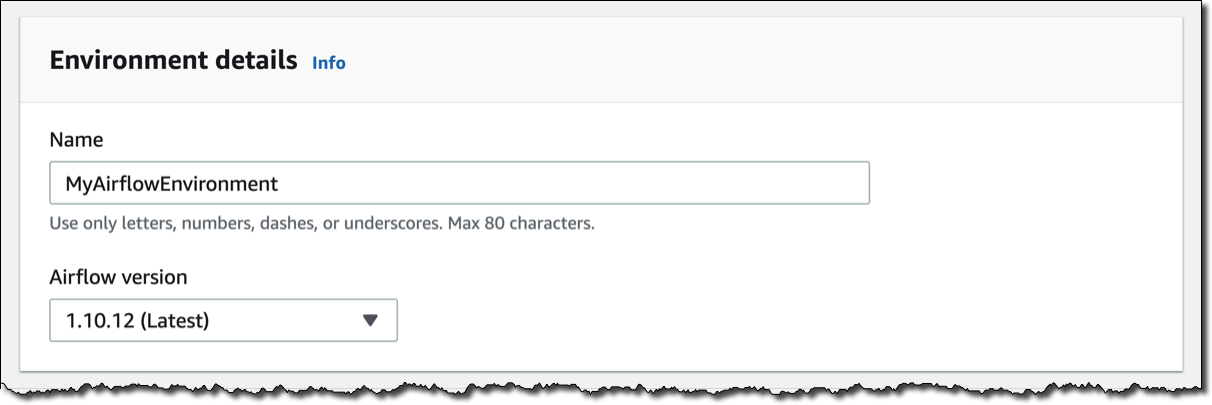
In the DataBrew console, I select the Projects tab and then Create project. I name the new project Comments. A new recipe is also created and will be automatically updated with the data transformations that I will apply next.

I choose to work on a New dataset and name it Comments.

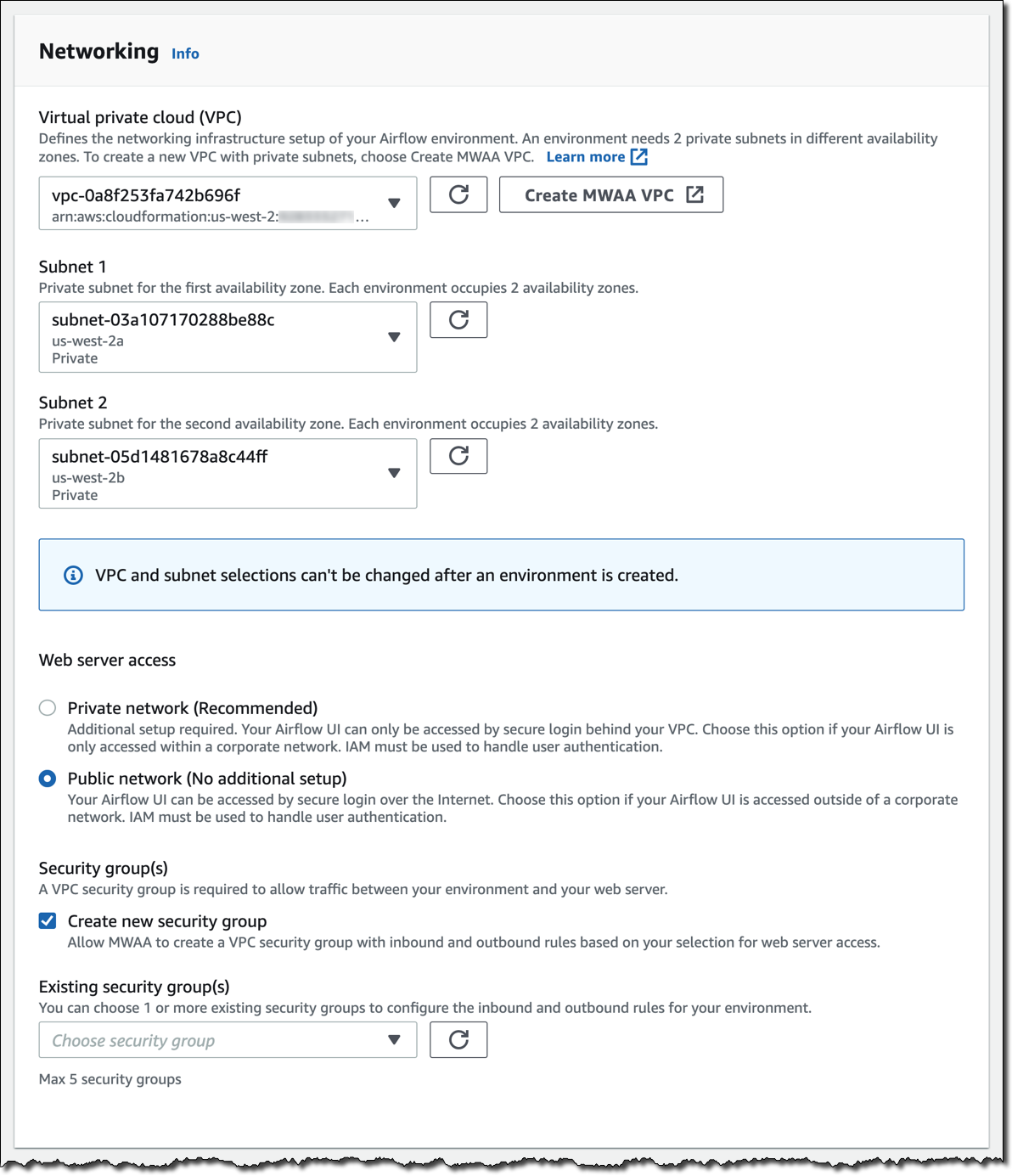
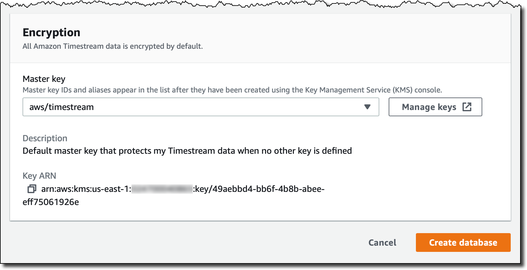
Here, I select Upload file and in the next dialog I upload a comments.csv file I prepared for this demo. In a production use case, here you will probably connect an existing source on S3 or in the Glue Data Catalog. For this demo, I specify the S3 destination for storing the uploaded file. I leave Encryption disabled.

The comments.csv file is very small, but will help show some common data preparation needs and how to complete them quickly with DataBrew. The format of the file is comma-separated values (CSV). The first line contains the name of the columns. Then, each line contains a text comment and a numerical rating made by a customer (customer_id) about an item (item_id). Each item is part of a category. For each text comment, there is an indication of the overall sentiment (comment_sentiment). Optionally, when giving the comment, customers can enable a flag to ask to be contacted for further support (support_needed).

Here’s the content of the comments.csv file:

customer_id,item_id,category,rating,comment,comment_sentiment,support_needed
234,2345,"Electronics;Computer", 5,"I love this!",Positive,False
321,5432,"Home;Furniture",1,"I can't make this work... Help, please!!!",negative,true
123,3245,"Electronics;Photography",3,"It works. But I'd like to do more",,True
543,2345,"Electronics;Computer",4,"Very nice, it's going well",Positive,False
786,4536,"Home;Kitchen",5,"I really love it!",positive,false
567,5432,"Home;Furniture",1,"I doesn't work :-(",negative,true
897,4536,"Home;Kitchen",3,"It seems OK...",,True
476,3245,"Electronics;Photography",4,"Let me say this is nice!",positive,false

In the Access permissions, I select a AWS Identity and Access Management (IAM) role which provides DataBrew read permissions to my input S3 bucket. Only roles where DataBrew is the service principal for the trust policy are shown in the DataBrew console. To create one in the IAM console, select DataBrew as trusted entity.

If the dataset is big, you can use Sampling to limit the number of rows to use in the project. These rows can be selected at the beginning, at the end, or randomly through the data. You are going to use projects to create recipes, and then jobs to apply recipes to all the data. Depending on your dataset, you may not need access to all the rows to define the data preparation recipe.

Optionally, you can use Tagging to manage, search, or filter resources you create with AWS Glue DataBrew.

The project is now being prepared and in a few minutes I can start exploring my dataset.

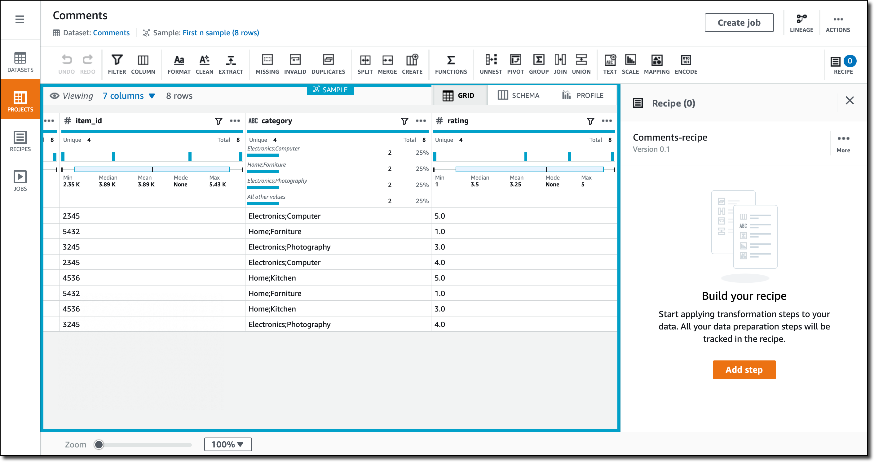
In the Grid view, the default when I create a new project, I see the data as it has been imported. For each column, there is a summary of the range of values that have been found. For numerical columns, the statistical distribution is given.

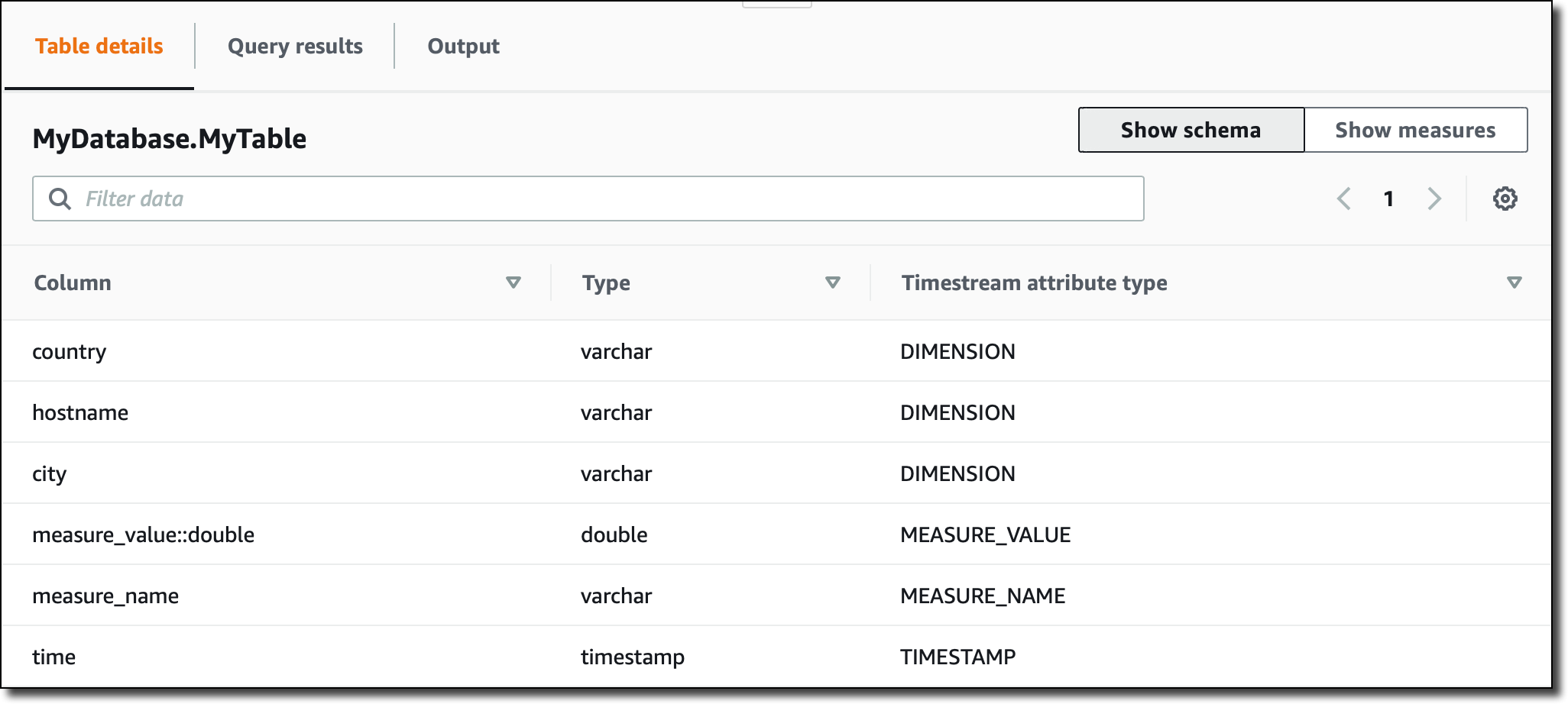
In the Schema view, I can drill down on the schema that has been inferred, and optionally hide some of the columns.

In the Profile view, I can run a data profile job to examine and collect statistical summaries about the data. This is an assessment in terms of structure, content, relationships, and derivation. For a large dataset, this is very useful to understand the data. For this small example the benefits are limited, but I run it nonetheless, sending the output of the profile job to a different folder in the same S3 bucket I use to store the source data.

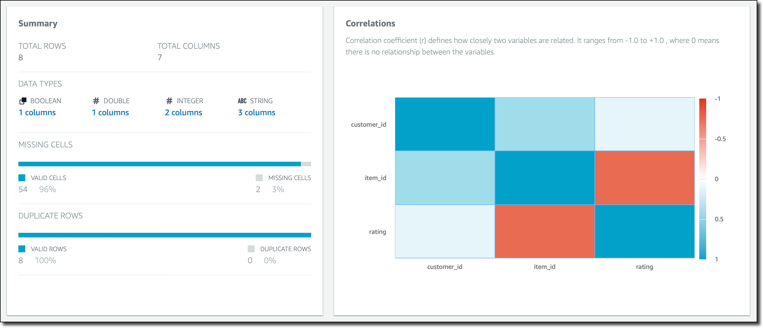
When the profile job has succeeded, I can see a summary of the rows and columns in my dataset, how many columns and rows are valid, and correlations between columns.

Here, if I select a column, for example rating, I can drill down into specific statistical information and correlations for that column.

Now, let’s do some actual data preparation. In the Grid view, I look at the columns. The category contains two pieces of information, separated by a semicolon. For example, the category of the first row is “Electronics;Computers.” I select the category column, then click on the column actions (the three small dots on the right of the column name) and there I have access to many transformations that I can apply to the column. In this case, I select to split the column on a single delimiter. Before applying the changes, I quickly preview them in the console.

I use the semicolon as delimiter, and now I have two columns, category_1 and category_2. I use the column actions again to rename them to category and subcategory. Now, for the first row, category contains Electronics and subcategory Computers. All these changes are added as steps to the project recipe, so that I’ll be able to apply them to similar data.

The rating column contains values between 1 and 5. For many algorithms, I prefer to have these kind of values normalized. In the column actions, I use min-max normalization to rescale the values between 0 and 1. More advanced techniques are available, such as mean or Z-score normalization. A new rating_normalized column is added.

I look into the recommendations that DataBrew gives for the comment column. Since it’s text, the suggestion is to use a standard case format, such as lowercase, capital case, or sentence case. I select lowercase.

The comments contain free text written by customers. To simplify further analytics, I use word tokenization on the column to remove stop words (such as “a,” “an,” “the”), expand contractions (so that “don’t” becomes “do not”), and apply stemming. The destination for these changes is a new column, comment_tokenized.

I still have some special characters in the comment_tokenized column, such as an emoticon :-). In the column actions, I select to clean and remove special characters.

I look into the recommendations for the comment_sentiment column. There are some missing values. I decide to fill the missing values with a neutral sentiment. Now, I still have values written with a different case, so I follow the recommendation to use lowercase for this column.

The comment_sentiment column now contains three different values (positive, negative, or neutral), but many algorithms prefer to have one-hot encoding, where there is a column for each of the possible values, and these columns contain 1, if that is the original value, or 0 otherwise. I select the Encode icon in the menu bar and then One-hot encode column. I leave the defaults and apply. Three new columns for the three possible values are added.

The support_needed column is recognized as boolean, and its values are automatically formatted to a standard format. I don’t have to do anything here.

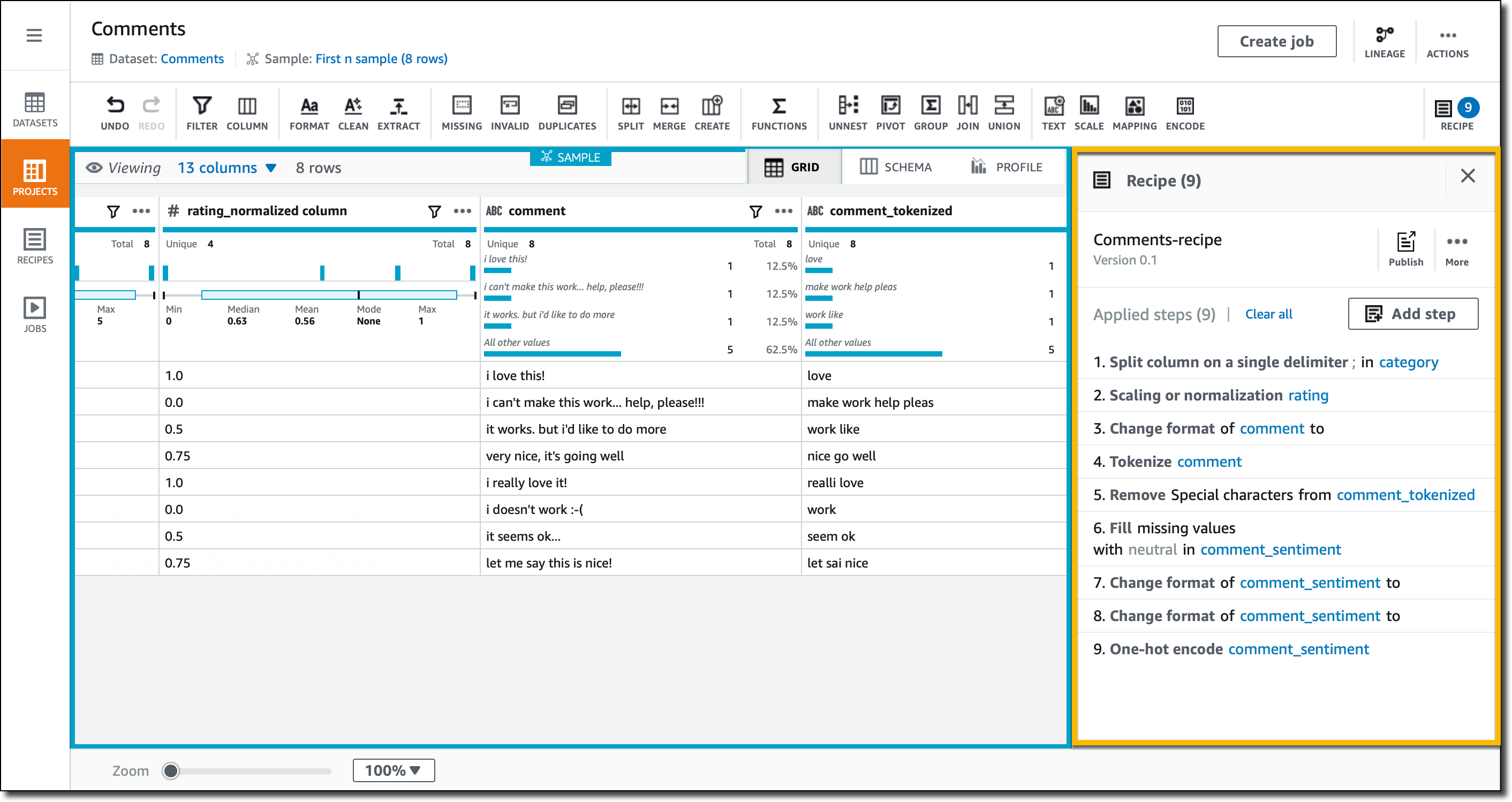
The recipe for my dataset is now ready to be published and can be used in a recurring job processing similar data. I didn’t have a lot of data, but the recipe can be used with much larger datasets.

In the recipe, you can find a list of all the transformations that I just applied. When running a recipe job, output data is available in S3 and ready to be used with analytics and machine learning platforms, or to build reports and visualization with BI tools. The output can be written in a different format than the input, for example using a columnar storage format like Apache Parquet.

Available Now

AWS Glue DataBrew is available today in US East (N. Virginia), US East (Ohio), US West (Oregon), Europe (Ireland), Europe (Frankfurt), Asia Pacific (Tokyo), Asia Pacific (Sydney).

It’s never been easier to prepare you data for analytics, machine learning, or for BI. In this way, you can really focus on getting the right insights for your business instead of writing custom code that you then have to maintain and update.

To practice with DataBrew, you can create a new project and select one of the sample datasets that are provided. That’s a great way to understand all the available features and how you can apply them to your data.

Learn more and get started with AWS Glue DataBrew today.

Danilo

New – Archive and Replay Events with Amazon EventBridge

Post Syndicated from Danilo Poccia original https://aws.amazon.com/blogs/aws/new-archive-and-replay-events-with-amazon-eventbridge/

Event-driven architectures use events to share information between the components of one or more applications. Events tell us that “something has happened”, maybe you received an API request, a file has been uploaded to a storage platform, or a database record has been updated. Business events describe something related to your activities, for example that […]

New – Application Load Balancer Support for End-to-End HTTP/2 and gRPC

Post Syndicated from Danilo Poccia original https://aws.amazon.com/blogs/aws/new-application-load-balancer-support-for-end-to-end-http-2-and-grpc/

Thanks to its efficiency and support for numerous programming languages, gRPC is a popular choice for microservice integrations and client-server communications. gRPC is a high performance remote procedure call (RPC) framework using HTTP/2 for transport and Protocol Buffers to describe the interface. To make it easier to use gRPC with your applications, Application Load Balancer (ALB) […]

Introducing Amazon SNS FIFO – First-In-First-Out Pub/Sub Messaging

Post Syndicated from Danilo Poccia original https://aws.amazon.com/blogs/aws/introducing-amazon-sns-fifo-first-in-first-out-pub-sub-messaging/

When designing a distributed software architecture, it is important to define how services exchange information. For example, the use of asynchronous communication decouples components and simplifies scaling, reducing the impact of changes and making it easier to release new features.

The two most common forms of asynchronous service-to-service communication are message queues and publish/subscribe messaging:

  • With message queues, messages are stored on the queue until they are processed and deleted by a consumer. On AWS, Amazon Simple Queue Service (SQS) provides a fully managed message queuing service with no administrative overhead.
  • With pub/sub messaging, a message published to a topic is delivered to all subscribers to the topic. On AWS, Amazon Simple Notification Service (SNS) is a fully managed pub/sub messaging service that enables message delivery to a large number of subscribers. Each subscriber can also set a filter policy to receive only the messages that it cares about.

You can use topics when you want to fan out messages to multiple applications, and queues when you want to send messages to one application. Using topics and queues together, you can decouple microservices, distributed systems, and serverless applications.

With SQS, you can use FIFO (First-In-First-Out) queues to preserve the order in which messages are sent and received, and to avoid that a message is processed more than once.

Introducing SNS FIFO Topics
Today, we are adding similar capabilities for pub/sub messaging with the introduction of SNS FIFO topics, providing strict message ordering and deduplicated message delivery to one or more subscribers.

FIFO topics manage ordering and deduplication similar to FIFO queues:

Ordering – You configure a message group by including a message group ID when publishing a message to a FIFO topic. For each message group ID, all messages are sent and delivered in order of their arrival. For example, to ensure the delivery of messages related to the same customer in order, you can publish these messages to the topic using the customer’s account number as the message group ID. There is no limit in the number of message groups with FIFO topics and queues. You don’t need to declare in advance the message group ID, any value will work. If you don’t have a logical distinction between messages, you can simply use the same message group ID for all and have a single group of ordered messages. The message group ID is passed to any subscribed FIFO queue.

Deduplication – Distributed systems (like SNS) and client applications sometimes generate duplicate messages. You can avoid duplicated message deliveries from the topic in two ways: either by enabling content-based deduplication on the topic, or by adding a deduplication ID to the messages that you publish. With message content-based deduplication, SNS uses a SHA-256 hash to generate the message deduplication ID using the body of the message. After a message with a specific deduplication ID is published successfully, there is a 5-minute interval during which any message with the same deduplication ID is accepted but not delivered. If you subscribe a FIFO queue to a FIFO topic, the deduplication ID is passed to the queue and it is used by SQS to avoid duplicate messages being received.

You can use FIFO topics and queues together to simplify the implementation of applications where the order of operations and events is critical, or when you cannot tolerate duplicates. For example, to process financial operations and inventory updates, or to asynchronously apply commands that you receive from a client device. FIFO queues can use message filtering in FIFO topics to selectively receive only a subset of messages rather than every message published to the topic.

How to Use SNS FIFO Topics
A common scenario where FIFO topics can help is when you receive updates that need to be processed in order. For example, I can use a FIFO topic to receive updates from an application where my customers edit their account profiles. Then, I subscribe an SQS FIFO queue to the FIFO topic, and use the queue as trigger for a Lambda function that applies the account updates to an Amazon DynamoDB table used by my Customer management system that needs to be kept in sync.

The decoupling introduced by the FIFO topic makes it easier to add new functionality with minimal impact to existing applications. For example, to reward my loyal customers with additional promotions, I add a new Loyalty application that is storing information in a relational database managed by Amazon Aurora. To keep the customer’s information stored in the Loyalty database in sync with my other applications, I can subscribe a new FIFO queue to the same FIFO topic, and add a new Lambda function that receives customer updates in the same order as they are generated, and applies them to the Loyalty database. In this way, I don’t need to change code and configuration of other applications to integrate the new Loyalty app.

First, I create two FIFO queues in the SQS console, leaving all options to their defaults:

  • The customer.fifo queue to process updates in my Customer management system.
  • The loyalty.fifo queue to help me collect and store customer updates for the Loyalty application.

In the SNS console, I create the updates.fifo topic. I select FIFO as type, and enable Content-based message deduplication.

Then,  I subscribe the customer.fifo and loyalty.fifo queues to the topic.

To be able to receive messages, I add a statement to the access policy of both queues granting the updates.fifo topic permissions to send messages to the queues. For example, for the customer.fifo queue the statement is:

{
  "Effect": "Allow",
  "Principal": {
    "Service": "sns.amazonaws.com"
  },
  "Action": "SQS:SendMessage",
  "Resource": "arn:aws:sqs:us-east-2:123412341234:customer.fifo",
  "Condition": {
    "ArnLike": {
      "aws:SourceArn": "arn:aws:sns:us-east-2:123412341234:updates.fifo"
    }
  }
}

Now, I use the SNS console to publish 4 messages in sequence. For all messages, I use the same message group ID. In this way, they are all in the same message group. The only part that is different is the message body, where I use in order:

  • Update One
  • Update Two
  • Update Three
  • Update One

In the SQS console, I see that only 3 messages have been delivered to the FIFO queues:

Why is that? When I created the FIFO topics, I enabled content-based deduplication. The 4 messages were sent within the 5-minute deduplication window. The last message has been recognized as a duplicate of the first one and has not been delivered to the subscribed queues.

Let’s see the actual messages in the queues. I use the AWS Command Line Interface (CLI) to receive the messages from SQS, and the jq command-line JSON processor to format the output and get only the Message in the Body.

Here are the messages in the customer.fifo queue:

$ aws sqs receive-message --queue-url https://sqs.us-east-2.amazonaws.com/123412341234/customer.fifo --max-number-of-messages 10 | jq '.Messages[].Body | fromjson | .Message'

"Update One"
"Update Two"
"Update Three"

And these are the messages in the loyalty.fifo queue:

$ aws sqs receive-message --queue-url https://sqs.us-east-2.amazonaws.com/123412341234/loyalty.fifo --max-number-of-messages 10 | jq '.Messages[].Body | fromjson | .Message'

"Update One"
"Update Two"
"Update Three"

As expected, the 3 messages with unique content have been delivered to both queues in the same order as they were sent.

Available Now
You can use SNS FIFO topics in all commercial regions. You can process up to 300 transactions per second (TPS) per FIFO topic or FIFO queue. With SNS, you pay only for what you use, you can find more information in the pricing page.

To learn more, please see the documentation.

Danilo

Store and Access Time Series Data at Any Scale with Amazon Timestream – Now Generally Available

Post Syndicated from Danilo Poccia original https://aws.amazon.com/blogs/aws/store-and-access-time-series-data-at-any-scale-with-amazon-timestream-now-generally-available/

Time series are a very common data format that describes how things change over time. Some of the most common sources are industrial machines and IoT devices, IT infrastructure stacks (such as hardware, software, and networking components), and applications that share their results over time. Managing time series data efficiently is not easy because the data model doesn’t fit general-purpose databases.

For this reason, I am happy to share that Amazon Timestream is now generally available. Timestream is a fast, scalable, and serverless time series database service that makes it easy to collect, store, and process trillions of time series events per day up to 1,000 times faster and at as little as to 1/10th the cost of a relational database.

This is made possible by the way Timestream is managing data: recent data is kept in memory and historical data is moved to cost-optimized storage based on a retention policy you define. All data is always automatically replicated across multiple availability zones (AZ) in the same AWS region. New data is written to the memory store, where data is replicated across three AZs before returning success of the operation. Data replication is quorum based such that the loss of nodes, or an entire AZ, does not disrupt durability or availability. In addition, data in the memory store is continuously backed up to Amazon Simple Storage Service (S3) as an extra precaution.

Queries automatically access and combine recent and historical data across tiers without the need to specify the storage location, and support time series-specific functionalities to help you identify trends and patterns in data in near real time.

There are no upfront costs, you pay only for the data you write, store, or query. Based on the load, Timestream automatically scales up or down to adjust capacity, without the need to manage the underlying infrastructure.

Timestream integrates with popular services for data collection, visualization, and machine learning, making it easy to use with existing and new applications. For example, you can ingest data directly from AWS IoT Core, Amazon Kinesis Data Analytics for Apache Flink, AWS IoT Greengrass, and Amazon MSK. You can visualize data stored in Timestream from Amazon QuickSight, and use Amazon SageMaker to apply machine learning algorithms to time series data, for example for anomaly detection. You can use Timestream fine-grained AWS Identity and Access Management (IAM) permissions to easily ingest or query data from an AWS Lambda function. We are providing the tools to use Timestream with open source platforms such as Apache Kafka, Telegraf, Prometheus, and Grafana.

Using Amazon Timestream from the Console
In the Timestream console, I select Create database. I can choose to create a Standard database or a Sample database populated with sample data. I proceed with a standard database and I name it MyDatabase.

All Timestream data is encrypted by default. I use the default master key, but you can use a customer managed key that you created using AWS Key Management Service (KMS). In that way, you can control the rotation of the master key, and who has permissions to use or manage it.

I complete the creation of the database. Now my database is empty. I select Create table and name it MyTable.

Each table has its own data retention policy. First data is ingested in the memory store, where it can be stored from a minimum of one hour to a maximum of a year. After that, it is automatically moved to the magnetic store, where it can be kept up from a minimum of one day to a maximum of 200 years, after which it is deleted. In my case, I select 1 hour of memory store retention and 5 years of magnetic store retention.

When writing data in Timestream, you cannot insert data that is older than the retention period of the memory store. For example, in my case I will not be able to insert records older than 1 hour. Similarly, you cannot insert data with a future timestamp.

I complete the creation of the table. As you noticed, I was not asked for a data schema. Timestream will automatically infer that as data is ingested. Now, let’s put some data in the table!

Loading Data in Amazon Timestream
Each record in a Timestream table is a single data point in the time series and contains:

  • The measure name, type, and value. Each record can contain a single measure, but different measure names and types can be stored in the same table.
  • The timestamp of when the measure was collected, with nanosecond granularity.
  • Zero or more dimensions that describe the measure and can be used to filter or aggregate data. Records in a table can have different dimensions.

For example, let’s build a simple monitoring application collecting CPU, memory, swap, and disk usage from a server. Each server is identified by a hostname and has a location expressed as a country and a city.

In this case, the dimensions would be the same for all records:

  • country
  • city
  • hostname

Records in the table are going to measure different things. The measure names I use are:

  • cpu_utilization
  • memory_utilization
  • swap_utilization
  • disk_utilization

Measure type is DOUBLE for all of them.

For the monitoring application, I am using Python. To collect monitoring information I use the psutil module that I can install with:

pip3 install psutil

Here’s the code for the collect.py application:

import time
import boto3
import psutil

from botocore.config import Config

DATABASE_NAME = "MyDatabase"
TABLE_NAME = "MyTable"

COUNTRY = "UK"
CITY = "London"
HOSTNAME = "MyHostname" # You can make it dynamic using socket.gethostname()

INTERVAL = 1 # Seconds

def prepare_record(measure_name, measure_value):
    record = {
        'Time': str(current_time),
        'Dimensions': dimensions,
        'MeasureName': measure_name,
        'MeasureValue': str(measure_value),
        'MeasureValueType': 'DOUBLE'
    }
    return record


def write_records(records):
    try:
        result = write_client.write_records(DatabaseName=DATABASE_NAME,
                                            TableName=TABLE_NAME,
                                            Records=records,
                                            CommonAttributes={})
        status = result['ResponseMetadata']['HTTPStatusCode']
        print("Processed %d records. WriteRecords Status: %s" %
              (len(records), status))
    except Exception as err:
        print("Error:", err)


if __name__ == '__main__':

    session = boto3.Session()
    write_client = session.client('timestream-write', config=Config(
        read_timeout=20, max_pool_connections=5000, retries={'max_attempts': 10}))
    query_client = session.client('timestream-query')

    dimensions = [
        {'Name': 'country', 'Value': COUNTRY},
        {'Name': 'city', 'Value': CITY},
        {'Name': 'hostname', 'Value': HOSTNAME},
    ]

    records = []

    while True:

        current_time = int(time.time() * 1000)
        cpu_utilization = psutil.cpu_percent()
        memory_utilization = psutil.virtual_memory().percent
        swap_utilization = psutil.swap_memory().percent
        disk_utilization = psutil.disk_usage('/').percent

        records.append(prepare_record('cpu_utilization', cpu_utilization))
        records.append(prepare_record(
            'memory_utilization', memory_utilization))
        records.append(prepare_record('swap_utilization', swap_utilization))
        records.append(prepare_record('disk_utilization', disk_utilization))

        print("records {} - cpu {} - memory {} - swap {} - disk {}".format(
            len(records), cpu_utilization, memory_utilization,
            swap_utilization, disk_utilization))

        if len(records) == 100:
            write_records(records)
            records = []

        time.sleep(INTERVAL)

I start the collect.py application. Every 100 records, data is written in the MyData table:

$ python3 collect.py
records 4 - cpu 31.6 - memory 65.3 - swap 73.8 - disk 5.7
records 8 - cpu 18.3 - memory 64.9 - swap 73.8 - disk 5.7
records 12 - cpu 15.1 - memory 64.8 - swap 73.8 - disk 5.7
. . .
records 96 - cpu 44.1 - memory 64.2 - swap 73.8 - disk 5.7
records 100 - cpu 46.8 - memory 64.1 - swap 73.8 - disk 5.7
Processed 100 records. WriteRecords Status: 200
records 4 - cpu 36.3 - memory 64.1 - swap 73.8 - disk 5.7
records 8 - cpu 31.7 - memory 64.1 - swap 73.8 - disk 5.7
records 12 - cpu 38.8 - memory 64.1 - swap 73.8 - disk 5.7
. . .

Now, in the Timestream console, I see the schema of the MyData table, automatically updated based on the data ingested:

Note that, since all measures in the table are of type DOUBLE, the measure_value::double column contains the value for all of them. If the measures were of different types (for example, INT or BIGINT) I would have more columns (such as measure_value::int and measure_value::bigint) .

In the console, I can also see a recap of which kind measures I have in the table, their corresponding data type, and the dimensions used for that specific measure:

Querying Data from the Console
I can query time series data using SQL. The memory store is optimized for fast point-in-time queries, while the magnetic store is optimized for fast analytical queries. However, queries automatically process data on all stores (memory and magnetic) without having to specify the data location in the query.

I am running queries straight from the console, but I can also use JDBC connectivity to access the query engine. I start with a basic query to see the most recent records in the table:

SELECT * FROM MyDatabase.MyTable ORDER BY time DESC LIMIT 8

Let’s try something a little more complex. I want to see the average CPU utilization aggregated by hostname in 5 minutes intervals for the last two hours. I filter records based on the content of measure_name. I use the function bin() to round time to a multiple of an interval size, and the function ago() to compare timestamps:

SELECT hostname,
       bin(time, 5m) as binned_time,
       avg(measure_value::double) as avg_cpu_utilization
  FROM MyDatabase.MyTable
 WHERE measure_name = 'cpu_utilization'
   AND time > ago(2h)
 GROUP BY hostname, bin(time, 5m)

When collecting time series data you may miss some values. This is quite common especially for distributed architectures and IoT devices. Timestream has some interesting functions that you can use to fill in the missing values, for example using linear interpolation, or based on the last observation carried forward.

More generally, Timestream offers many functions that help you to use mathematical expressions, manipulate strings, arrays, and date/time values, use regular expressions, and work with aggregations/windows.

To experience what you can do with Timestream, you can create a sample database and add the two IoT and DevOps datasets that we provide. Then, in the console query interface, look at the sample queries to get a glimpse of some of the more advanced functionalities:

Using Amazon Timestream with Grafana
One of the most interesting aspects of Timestream is the integration with many platforms. For example, you can visualize your time series data and create alerts using Grafana 7.1 or higher. The Timestream plugin is part of the open source edition of Grafana.

I add a new GrafanaDemo table to my database, and use another sample application to continuously ingest data. The application simulates performance data collected from a microservice architecture running on thousands of hosts.

I install Grafana on an Amazon Elastic Compute Cloud (EC2) instance and add the Timestream plugin using the Grafana CLI.

$ grafana-cli plugins install grafana-timestream-datasource

I use SSH Port Forwarding to access the Grafana console from my laptop:

$ ssh -L 3000:<EC2-Public-DNS>:3000 -N -f ec2-user@<EC2-Public-DNS>

In the Grafana console, I configure the plugin with the right AWS credentials, and the Timestream database and table. Now, I can select the sample dashboard, distributed as part of the Timestream plugin, using data from the GrafanaDemo table where performance data is continuously collected:

Available Now
Amazon Timestream is available today in US East (N. Virginia), Europe (Ireland), US West (Oregon), and US East (Ohio). You can use Timestream with the console, the AWS Command Line Interface (CLI), AWS SDKs, and AWS CloudFormation. With Timestream, you pay based on the number of writes, the data scanned by the queries, and the storage used. For more information, please see the pricing page.

You can find more sample applications in this repo. To learn more, please see the documentation. It’s never been easier to work with time series, including data ingestion, retention, access, and storage tiering. Let me know what you are going to build!

Danilo

New EC2 T4g Instances – Burstable Performance Powered by AWS Graviton2 – Try Them for Free

Post Syndicated from Danilo Poccia original https://aws.amazon.com/blogs/aws/new-t4g-instances-burstable-performance-powered-by-aws-graviton2/

Two years ago Amazon Elastic Compute Cloud (EC2) T3 instances were first made available, offering a very cost effective way to run general purpose workloads. While current T3 instances offer sufficient compute performance for many use cases, many customers have told us that they have additional workloads that would benefit from increased peak performance and lower cost.

Today, we are launching T4g instances, a new generation of low cost burstable instance type powered by AWS Graviton2, a processor custom built by AWS using 64-bit Arm Neoverse cores. Using T4g instances you can enjoy a performance benefit of up to 40% at a 20% lower cost in comparison to T3 instances, providing the best price/performance for a broader spectrum of workloads.

T4g instances are designed for applications that don’t use CPU at full power most of the time, using the same credit model as T3 instances with unlimited mode enabled by default. Examples of production workloads that require high CPU performance only during times of heavy data processing are web/application servers, small/medium data stores, and many microservices. Compared to previous generations, the performance of T4g instances makes it possible to migrate additional workloads such as caching servers, search engine indexing, and e-commerce platforms.

T4g instances are available in 7 sizes providing up to 5 Gbps of network and up to 2.7 Gbps of Amazon Elastic Block Store (EBS) performance:

Name vCPUs Baseline Performance/vCPU CPU Credits Earned/Hour Memory
t4g.nano 2 5% 6 0.5 GiB
t4g.micro 2 10% 12 1 GiB
t4g.small 2 20% 24 2 GiB
t4g.medium 2 20% 24 4 GiB
t4g.large 2 30% 36 8 GiB
t4g.xlarge 4 40% 96 16 GiB
t4g.2xlarge 8 40% 192 32 GiB

Free Trial
To make it easier to develop, test, and run your applications on T4g instances, all AWS customers are automatically enrolled in a free trial on the t4g.micro size. Starting September 2020 until December 31st 2020, you can run a t4g.micro instance and automatically get 750 free hours per month deducted from your bill, including any CPU credits during the free 750 hours of usage. The 750 hours are calculated in aggregate across all regions. For details on terms and conditions of the free trial, please refer to the EC2 FAQs.

During the free trial, have a look at this getting started guide on using the Arm-based AWS Graviton processors. There, you can find suggestions on how to build and optimize your applications, using different programming languages and operating systems, and on managing container-based workloads. Some of the tips are specific for the Graviton processor, but most of the content works generally for anyone using Arm to run their code.

Using T4g Instances
You can start an EC2 instance in different ways, for example using the EC2 console, the AWS Command Line Interface (CLI), AWS SDKs, or AWS CloudFormation. For my first T4g instance, I use the AWS CLI:

$ aws ec2 run-instances \
  --instance-type t4g.micro \
  --image-id ami-09a67037138f86e67 \
  --security-groups MySecurityGroup \
  --key-name my-key-pair

The Amazon Machine Image (AMI) I am using is based on Amazon Linux 2. Other platforms are available, such as Ubuntu 18.04 or newer, Red Hat Enterprise Linux 8.0 and newer, and SUSE Enterprise Server 15 and newer. You can find additional AMIs in the AWS Marketplace, for example Fedora, Debian, NetBSD, CentOS, and NGINX Plus. For containerized applications, Amazon ECS and Amazon Elastic Kubernetes Service optimized AMIs are available as well.

The security group I selected gives me SSH access to the instance. I connect to the instance and do a general update:

$ sudo yum update -y

Since the kernel has been updated, I reboot the instance.

I’d like to set up this instance as a development environment. I can use it to build new applications, or to recompile my existing apps to the 64-bit Arm architecture. To install most development tools, such as Git, GCC, and Make, I use this group of packages:

$ sudo yum groupinstall -y "Development Tools"

AWS is working with several open source communities to drive improvements to the performance of software stacks running on AWS Graviton2. For example, you can see our contributions to PHP for Arm64 in this post.

Using the latest versions helps you obtain maximum performance from your Graviton2-based instances. The amazon-linux-extras command enables new versions for some of my favorite programming environments:

$ sudo amazon-linux-extras enable golang1.11 corretto8 php7.4 python3.8 ruby2.6

The output of the amazon-linux-extras command tells me which packages to install with yum:

$ yum clean metadata
$ sudo yum install -y golang java-1.8.0-amazon-corretto \
  php-cli php-pdo php-fpm php-json php-mysqlnd \
  python38 ruby ruby-irb rubygem-rake rubygem-json rubygems

Let’s check the versions of the tools that I just installed:

$ go version
go version go1.13.14 linux/arm64
$ java -version
openjdk version "1.8.0_265"
OpenJDK Runtime Environment Corretto-8.265.01.1 (build 1.8.0_265-b01)
OpenJDK 64-Bit Server VM Corretto-8.265.01.1 (build 25.265-b01, mixed mode)
$ php -v
PHP 7.4.9 (cli) (built: Aug 21 2020 21:45:13) ( NTS )
Copyright (c) The PHP Group
Zend Engine v3.4.0, Copyright (c) Zend Technologies
$ python3.8 -V
Python 3.8.5
$ ruby -v
ruby 2.6.3p62 (2019-04-16 revision 67580) [aarch64-linux]

It looks like I am ready to go! Many more packages are available with yum, such as MariaDB and PostgreSQL. If you’re interested in databases, you might also want to try the preview of Amazon RDS powered by AWS Graviton2 processors.

Available Now
T4g instances are available today in US East (N. Virginia, Ohio), US West (Oregon), Asia Pacific (Tokyo, Mumbai), Europe (Frankfurt, Ireland).

You now have a broad choice of Graviton2-based instances to better optimize your workloads for cost and performance: low cost burstable general-purpose (T4g), general purpose (M6g), compute optimized (C6g) and memory optimized (R6g) instances. Local NVMe-based SSD storage options are also available.

You can use the free trial to develop new applications, or migrate your existing workloads to the AWS Graviton2 processor. Let me know how that goes!

Danilo

AWS Named as a Cloud Leader for the 10th Consecutive Year in Gartner’s Infrastructure & Platform Services Magic Quadrant

Post Syndicated from Danilo Poccia original https://aws.amazon.com/blogs/aws/aws-named-as-a-cloud-leader-for-the-10th-consecutive-year-in-gartners-infrastructure-platform-services-magic-quadrant/

At AWS, we strive to provide you a technology platform that allows for agile development, rapid deployment, and unlimited scale, so that you can free up your resources to focus on innovation for your customers. It’s greatly rewarding to see our efforts recognized not just by our customers, but also by leading analysts.

This year, Gartner announced a new Magic Quadrant for Cloud Infrastructure and Platform Services (CIPS). This is an evolution of their Magic Quadrant for Cloud Infrastructure as a Service (IaaS) for which AWS has been named as a Leader for nine consecutive years.

Customers are using the cloud in broad ways, beyond foundational compute, networking and storage services. We believe for this reason, Gartner is expanding the scope to include additional platform as a service (PaaS) capabilities, and is extending coverage for areas such as managed database services, serverless computing, and developer tools.

Today, I am happy to share that AWS has been named as a Leader in the Magic Quadrant for Cloud Infrastructure and Platform Services, and placed highest in Ability to Execute and furthest in Completeness of Vision.

More information on the features and factors that our customers examine when choosing a cloud provider are available in the full report.

Danilo

Gartner, Magic Quadrant for Cloud Infrastructure and Platform Services, Raj Bala, Bob Gill, Dennis Smith, David Wright, Kevin Ji, 1 September 2020 – Gartner does not endorse any vendor, product or service depicted in its research publications, and does not advise technology users to select only those vendors with the highest ratings or other designation. Gartner research publications consist of the opinions of Gartner’s research organization and should not be construed as statements of fact. Gartner disclaims all warranties, expressed or implied, with respect to this research, including any warranties of merchantability or fitness for a particular purpose.