Post Syndicated from Betty Zheng (郑予彬) original https://aws.amazon.com/blogs/aws/aws-weekly-roundup-amazon-q-business-is-hipaa-eligible-amazon-dcv-aws-repost-agent-and-more-oct-07-2024/
Last Friday, I had the privilege of attending China Engineer’s Day 2024(CED 2024) in Hangzhou as the Amazon Web Services (AWS) speaker. The event was organized by the China Computer Federation (CCF), one of the most influential professional developer communities in China.
At CED 2024, I spoke about how AI development tools can improve developer productivity. I was honored to receive a certificate of excellence from CCF, and Amazon Q garnered significant attention from the attendees.

Now, let’s turn to other exciting news in the AWS universe from last week.
Last week’s launches
Here are some launches that got my attention:
Amazon Q Business is now HIPAA eligible – Amazon Q business has received Health Insurance Portability and Accountability Act (HIPAA) certification. This means healthcare and life sciences organizations such as health insurance companies and healthcare providers can now use Amazon Q Business to run sensitive workloads regulated under the US HIPAA law.
NICE DCV renames to Amazon DCV – NICE DCV is rebranded to Amazon DCV. This high performance remote display protocol allows secure delivery of remote desktops and application streaming from any cloud or data center to any device, even over varying network conditions. Amazon DCV supports both Windows and major Linux distributions on the server side. Clients can use native DCV client for Windows, Linux, or macOS, as well as web browsers, to receive desktops and application streamings. The DCV server and client only transfer encrypted pixels, not data, ensuring no confidential information is downloaded. When using Amazon DCV on AWS with Amazon Elastic Compute Cloud (Amazon EC2), you can take advantage of the AWS 108 Availability Zones across the 33 geographic Regions and 31 local zones. The 2024.0 release now supports the latest Ubuntu 24.04 LTS. For more details, check out Sébastien Stormacq’s new launch blog post.
AWS re:Post launches re:Post Agent – AWS re:Post provides access to curated knowledge and a vibrant community that helps users become even more successful on AWS. re:Post Agent is a generative AI assistant designed to provide rapid, intelligent responses to questions in the re:Post community. It expands the available AWS knowledge base, and community experts will earn reputation points by reviewing the AI-generated answers.
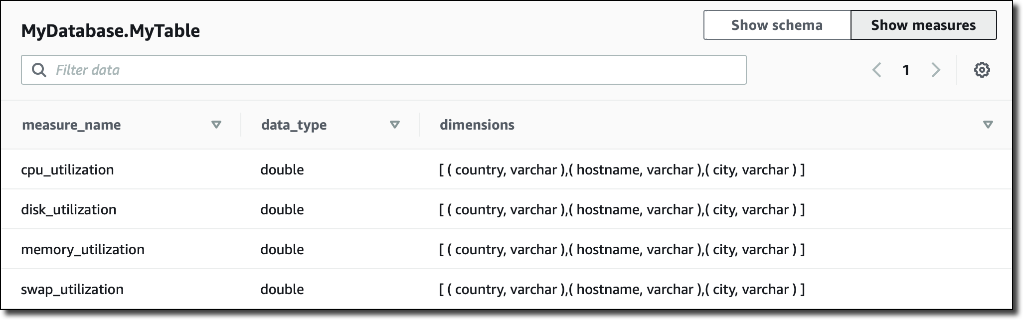
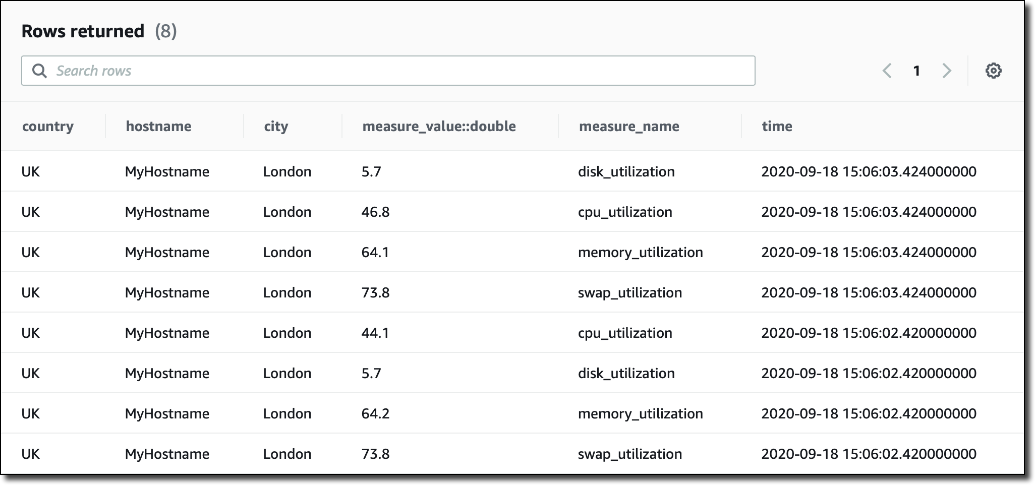
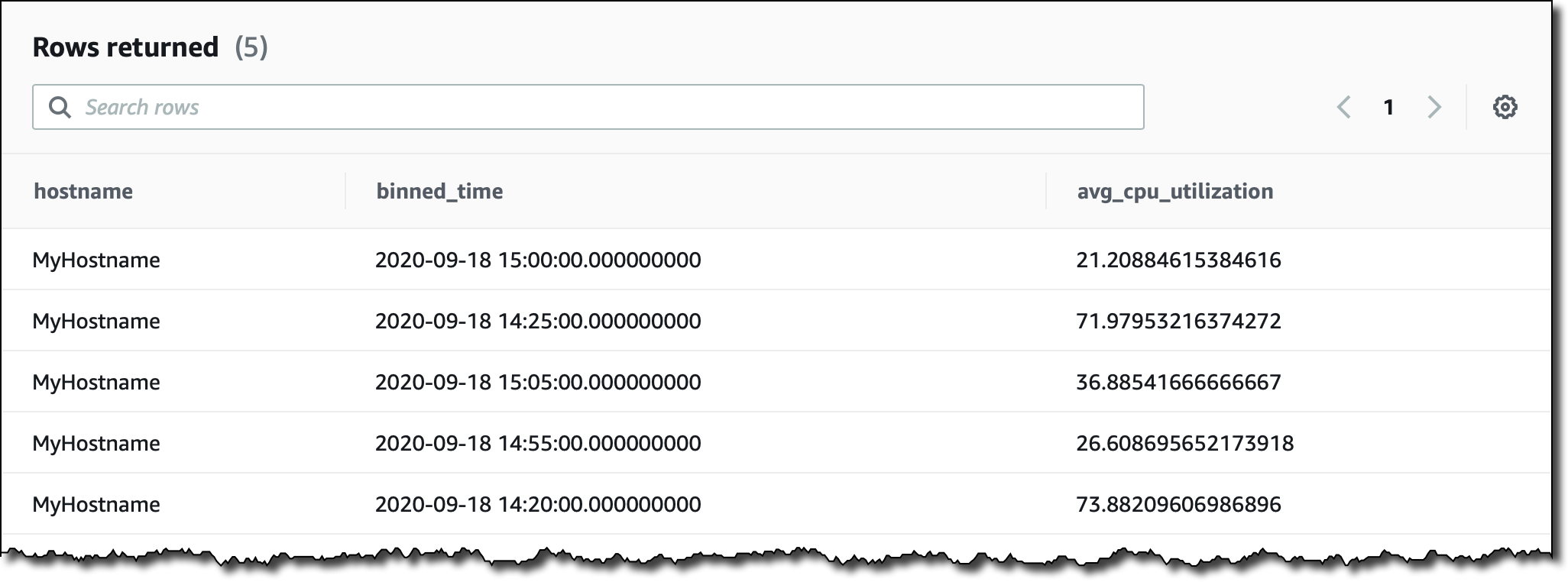
Advanced configuration with Amazon Timestream for InfluxDB – This new launch introduces a feature that allows uses to monitor instance CPU, memory, and disk utilization metrics directly from the AWS Management Console.
A new stop ingestion API of Amazon Bedrock Knowledge Bases – This new API allows users to halt ongoing ingestion jobs at will. Providing greater control over data ingestion workflows, users can quickly stop accidental or unwanted ingestion processes without waiting for completion. By using the new StopIngestionJob API, you can respond rapidly to evolving needs and potentially reduce costs. This capability is available across all AWS Regions where Amazon Bedrock Knowledge Bases are offered.
Higher storage limit of Amazon AppStream 2.0 – Amazon AppStream 2.0 has expanded the default size limit for application settings persistence from 1 GB to 5 GB. This increase allows end users to store more application data and settings without manual intervention and without affecting performance or session setup time.
There were over 40 launches and releases last week. It was difficult for me to select the important ones. In addition to those already mentioned, here’s a list of potentially important feature updates:
- Amazon Aurora Serverless v2 now supports up to 256 ACUs
- Amazon Aurora MySQL now supports RDS Data API
- Amazon Aurora supports PostgreSQL 16.4, 15.8, 14.13, 13.16, and 12.20
- Amazon Redshift now offers the RA3.large instance.
For a full list of AWS announcements, be sure to keep an eye on AWS’s What’s New Feed page.
Other AWS news
Here are some other noteworthy items from last week.
 Amazon WorkSpaces Thin Client – Amazon WorkSpaces Thin Client inventory is now available to purchase in the UK on Amazon Business, in addition to the US, France, Germany, Italy, and Spain. It’s a sleek, cost-effective device that brings secure access to AWS end user computing services right to your fingertips. This nifty gadget is like a digital fortress, preventing unauthorized data storage and applications, while giving IT admins the tools to manage and monitor their fleet of thin clients with ease.
Helping communities impacted by Hurricane Helene – AWS Disaster Response team is working closely with local partners and humanitarian organizations to deliver critical supplies to those in need in the Southeast. We’re also deploying AWS technology to help with re-connectivity, aid relief operations on the ground, and support food distribution needs in the region.
The life of a prescription at Amazon Pharmacy – Read the Amazon Pharmacy AI use case to remove the complexity of the process of dispensing medications and improve patients’ experiences. The system transcribes raw prescription data into standardized formats, transforms medical abbreviations into full-text equivalents, and validates medication details against an industry database. This automated process, followed by pharmacist review, has reduced potential medication errors by 50 percent and improved processing speed by up to 90 percent, allowing pharmacists to focus on critical tasks and personalized care.
A thought leadership article on generative AI in the WIRED magazine – Read Antje‘s news column in Wired. It discusses how AWS opens the transformative power of AI to organizations of any size and level of experience. I recommend it to all AI enthusiasts and business innovators. AWS is on a mission to bring generative AI magic to businesses of all sizes, offering a buffet of AI tools for tech wizards and newcomers alike. Whether you’re a startup with big dreams or a corporate giant looking to stay ahead, AWS is rolling out the red carpet to the AI revolution. Don’t miss this chance to turn your wildest tech fantasies into reality!
Upcoming AWS events
Check your calendars and sign up for these AWS events:
AWS re:Invent 2024 – Registration is now open for the annual tech extravaganza, taking place December 2 – 6 in Las Vegas. I’m eager to learn about the new launches and excited to contribute to two chalk talks focusing on security topics (Dev311 – Enhance code security with generative AI and SEC228 – Navigate multi-level protection scheme compliance in AWS China Regions).
AWS Innovate Migrate, Modernize, and Build – Whether you are new to the cloud or an experienced user, you will learn something new at AWS Innovate. This is a free online conference. Register at a time and region convenient to North America (October 15), or Europe, Middle East & Africa (October 24).
AWS Community Days – Join community-led conferences featuring technical discussions, workshops, and hands-on labs led by expert AWS users and industry leaders from around the world. Don’t miss out on the AWS Community Days happening on October 12 in Sofia and October 19 in Vadodara, Spain, and Guatemala.
Browse more upcoming AWS led in-person and virtual events and developer-focused events.
That’s all for this week. Check back next Monday for another Weekly Roundup!
— Betty
This post is part of our Weekly Roundup series. Check back each week for a quick roundup of interesting news and announcements from AWS!