At the 39th
Chaos Communication Congress (39C3) in December, researchers Lexi
Groves (“49016”) and Liam Wachter said that they had discovered a
number of flaws in popular implementations of OpenPGP email-encryption standard. They also released an
accompanying web site, gpg.fail, with
descriptions of the discoveries. Most of those
presented were found in GNU Privacy
Guard (GPG), though the pair also discussed problems in age, Minisign, Sequoia, and the OpenPGP
standard (RFC 9580) itself. The discoveries have spurred some interesting
discussions and as well as responses from GPG and Sequoia
developers.
Security updates have been issued by AlmaLinux (brotli and container-tools:rhel8), Debian (python-keystonemiddleware and python3.9), Fedora (cef, freerdp, golang-github-tetratelabs-wazero, and libpcap), Oracle (brotli, gpsd, kernel, and transfig), Red Hat (freerdp, golang, java-11-openjdk with Extended Lifecycle Support, libpng, libssh, mingw-libpng, and runc), SUSE (abseil-cpp, alloy, apache2, bind, cpp-httplib, curl, erlang, firefox, gpg2, grafana, haproxy, hauler, hawk2, libblkid-devel, libpng16, libraylib550, python-keystonemiddleware-doc, python-uv, python-weasyprint, squid, and tomcat), and Ubuntu (crawl and iperf3).
Organizations increasingly rely on Microsoft as their foundational productivity and security technology provider. As these environments grow in scale and complexity, security leaders are responsible for operationalizing the vast signals traversing their Microsoft stack in order to anticipate and preempt threats. At the same time, those efforts must deliver measurable security outcomes and clear return on investment.
If you’re reading this, you already know what’s at stake. But I’ll say it louder for the folks in the back: As more of your environment consolidates onto Microsoft, the attack surface evolves – and without fully operationalizing that ecosystem, risk grows alongside it. We are excited to announce the availability of Rapid7 MDR for Microsoft – a preemptive threat detection, investigation, and response service that brings together Rapid7’s global SOC, our market-leading SIEM technology, and deeper bi-directional Microsoft Defender integrations. The service helps security and IT teams maximize their investments, reduce cost and complexity, respond decisively to threats, and improve their security posture and resilience.
Extend the power of your stack
Microsoft Defender provides broad visibility across modern environments – from endpoint and identity to cloud and email. That visibility leads many organizations to a fine line, where it can either mean rich, actionable insight for some security teams, and overwhelming signal volume and missed alerts for others. Rapid7 helps organizations build a clear picture from the rich telemetry by bringing these Microsoft signals together with our native telemetry. And by incorporating exposure and asset risk directly into investigations, our SOC is empowered to anticipate likely breach paths and intervene earlier in the attack lifecycle. Combining your Microsoft security stack with our preemptive MDR ultimately helps you:
Maximize the return on your existing Microsoft investments
Reduce the cost and operational burden associated with managing a SIEM
Gain the confidence that threats will be contained and neutralized
Improve the long-term posture and resilience of your security program
Capabilities that drive real-world outcomes
Leaning into Rapid7’s proven record as a leader in managed detection and response, MDR for Microsoft combines powerful AI-SOC technology with expert human service delivery to help Microsoft-centric organizations achieve measurable security outcomes. In IDC’s recent Business Value of Rapid7 MDR study, customers achieved a 422% three-year ROI, identified threats 87% faster, and reduced the likelihood of a major security event by 54%. MDR for Microsoft delivers these same results through capabilities designed to operationalize and protect Microsoft environments at scale, including:
Risk-aware analysis that stops attacks earlier: By pairing enterprise vulnerability risk management with analysis of live threat activity, the service preemptively identifies the attack paths most likely to be exploited – empowering efficient analyst evaluation with a clear understanding of underlying asset context.
Dedicated cybersecurity advisor extends your team: Your advisor leverages their practitioner experience to provide regular threat briefings, environment-hardening advice, program governance, and health checks – helping drive long-term maturity without adding headcount.
Decisive response backed by deep forensics and unlimited IR: Remote containment, endpoint forensics powered by our open-source DFIR framework – Velociraptor – and unlimited incident response ensure threats are stopped quickly, and fully investigated and neutralized before our team rests.
Unlimited log ingestion delivers predictable value: Remove SIEM cost constraints and ensure complete visibility so investigations are never limited by data volume or surprise overage fees.
Bi-Directional Defender integration that reduces friction: Endpoint alerts and analyst actions stay synchronized between Rapid7 and Microsoft consoles, keeping systems aligned while laying the foundation for broader integrations across additional Microsoft security vectors.
Always-on, expert-led SOC coverage: Our 24x7x365 global SOC continuously monitors and investigates activity across Microsoft and non-Microsoft environments, ensuring threats are identified and acted on as soon as they emerge.
Full transparency into SOC activity and outcomes: With direct access to the SIEM and investigation workflows, your team can ride sidecar on investigations, run your own queries, upskill internal teams, and clearly see the outcomes being delivered by the Rapid7 SOC over time.
Additional value-drivers included in the service are unlimited SOAR automation, standard 13-month data retention with the ability to extend, proactive threat hunting, and AI-assisted investigation workflows, delivering a comprehensive MDR experience that scales with your environment and outpaces attackers.
Make the most of Microsoft Defender with Rapid7
As Microsoft continues to serve as the backbone of modern environments, the ability to translate security signals into consistent action becomes increasingly critical. MDR for Microsoft is designed to help security leaders move confidently from visibility to outcomes – pairing the strength of Microsoft Defender with Rapid7’s proven expertise, preemptive risk-awareness, and resilience-building capabilities. The result is a security program that not only sees more, but responds faster, operates with greater confidence, and proves its value as environments continue to scale.
If you’d like to see how MDR for Microsoft can help you operationalize your Microsoft security stack, request a demo or reach out to your Rapid7 account team to continue the conversation.
No matter how many times we say it, the idea comes back again and again. Hopefully, this letter will hold back the tide for at least a while longer.
Executive summary: Scientists have understood for many years that internet voting is insecure and that there is no known or foreseeable technology that can make it secure. Still, vendors of internet voting keep claiming that, somehow, their new system is different, or the insecurity doesn’t matter. Bradley Tusk and his Mobile Voting Foundation keep touting internet voting to journalists and election administrators; this whole effort is misleading and dangerous.
At Grab, we’ve been exploring ways to dramatically reduce container startup times for our data platforms. Large container images for services like Airflow and Spark Connect were taking minutes to download, causing slow cold starts and poor auto-scaling performance. This blog post shares our journey implementing Docker image lazy loading using eStargz and Seekable OCI (SOCI) technologies, the results we achieved, and the lessons learned along the way.
Results: The numbers speak for themselves
Benchmark results
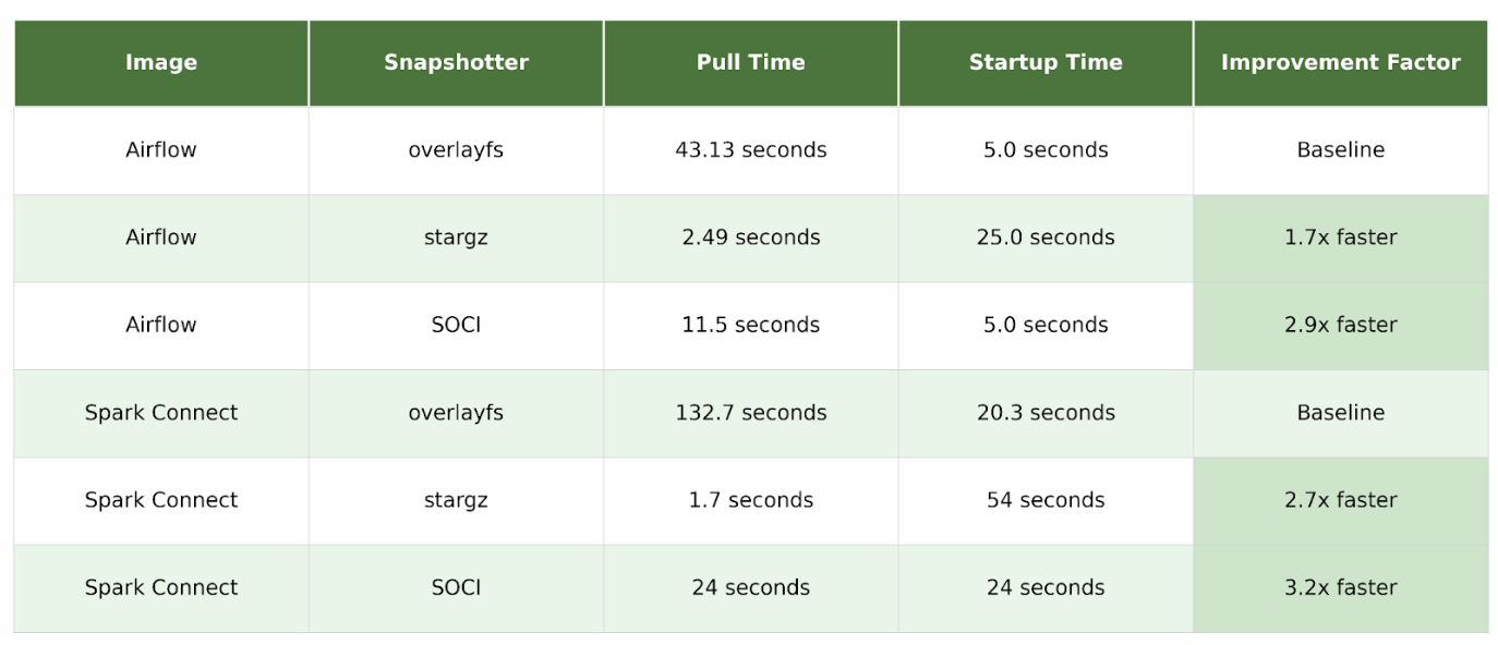
Our initial testing on fresh nodes (nodes without cached images) showed dramatic improvements in image pull times as shown in Figure 1.
Figure 1. Table of results.
The key advantage of lazy loading is the reduction in image pull time, especially on “fresh” nodes that do not have the image cached. By analyzing detailed pod events, we can see the precise impact of using the stargz snapshotter.
During our SOCI benchmark testing, we observed an important distinction between SOCI and eStargz: SOCI maintains the same application startup time as standard images, while eStargz takes longer. For example, with Airflow, both overlayFS and SOCI achieved 5.0 seconds startup time, while eStargz took 25.0 seconds. This demonstrates that lazy loading doesn’t eliminate download time; it redistributes it. SOCI’s approach of maintaining separate indexes allows it to optimize the download-to-startup time trade-off more effectively, keeping application startup performance on par with standard images while still dramatically reducing image pull time.
Production performance
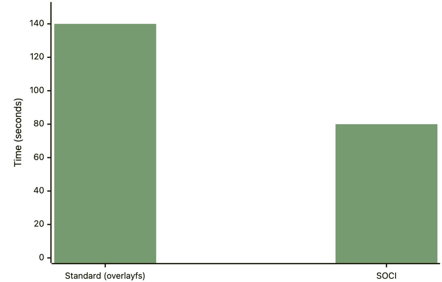
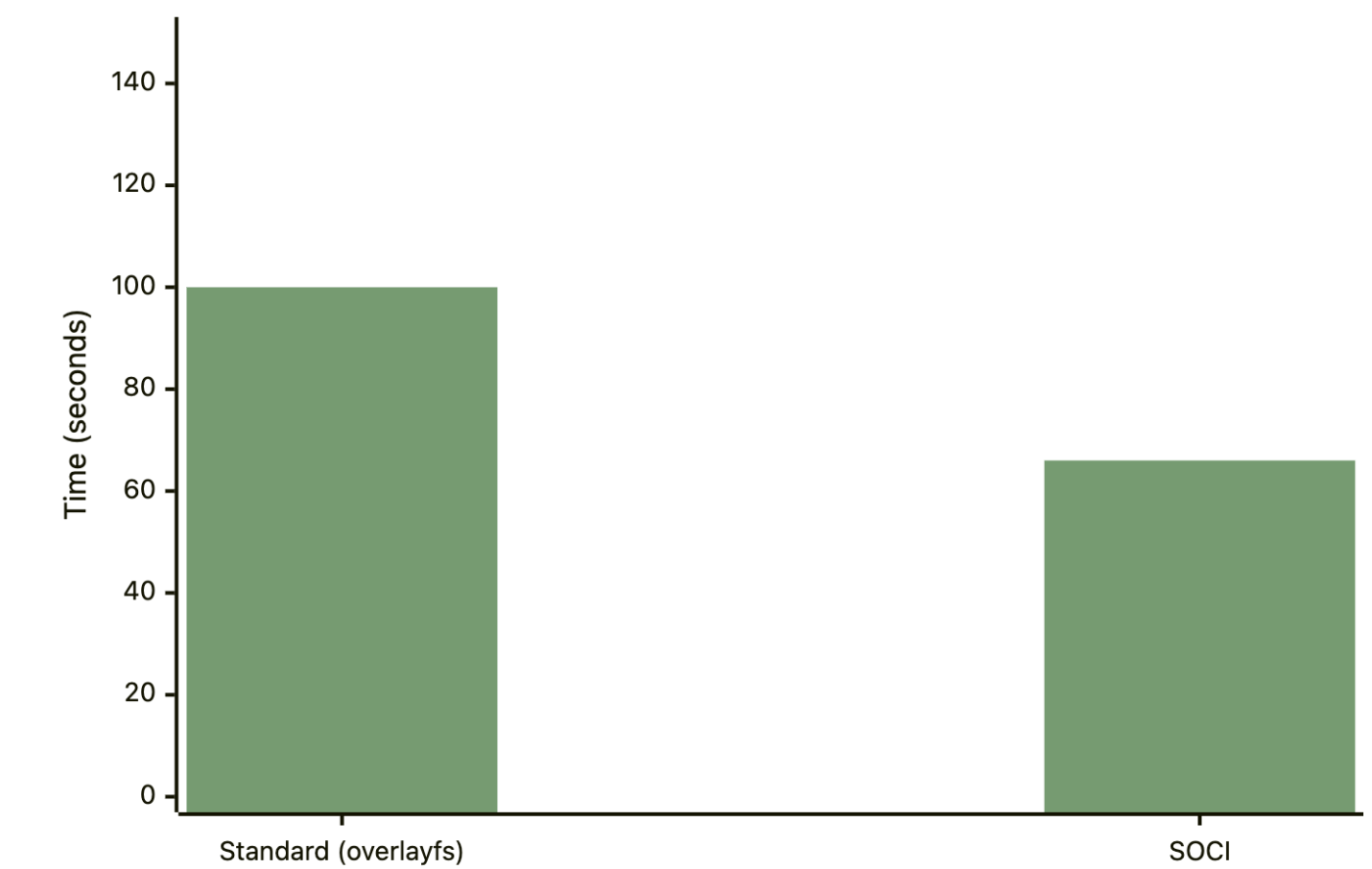
The production deployment of SOCI lazy loading has delivered significant, measurable improvements across our data platforms. Both Airflow and Spark Connect now experience 30-40% faster startup times, directly improving our ability to handle traffic spikes and scale efficiently. These improvements translate to better auto-scaling responsiveness, reduced resource waste during initialization, and improved user experience for data processing workloads. The sustained performance gains observed over time demonstrate that lazy loading is a stable, production-ready optimization that delivers consistent value.
Figure 2 and 3 illustrates the P95 startup time improvements for both services:
Figure 2. Production results: Airflow P95 startup time.
Figure 3. Production results: Spark Connect P95 startup time.
It is important to note that P95 startup time includes both the image download/pull time and the application startup time itself. This metric captures the entire system performance for both cold and hot starts on fresh and hot nodes, showing the overall system improvement rather than just cold start performance.
During the production deployment and monitoring, we gained valuable insights on SOCI configuration tuning. Following AWS’s recommended configuration from their blog on Introducing Seekable OCI: Parallel Pull Mode for Amazon EKS, we optimized our SOCI snapshotter settings:
Increased max_concurrent_downloads_per_image from 5 to 10.
Increased max_concurrent_unpacks_per_image from 3 to 10.
Increased concurrent_download_chunk_size from 8MB to 16MB (aligning with AWS’s recommendation for Elastic Container Registry (ECR)).
This configuration tuning led to a significant performance improvement: image download time on a fresh node was reduced from 60 seconds to 24 seconds, representing a 60% improvement. The key lesson here is that default SOCI configurations may not be optimal for all environments, and tuning these parameters based on your infrastructure (especially when using ECR) can yield substantial gains.
Technical background: How Docker lazy loading works
Container root filesystem (rootfs) and file organization
A container’s root filesystem, or rootfs, is the directory structure that the container sees as its root (/). It contains all the files and directories necessary for an application to run, including the application itself, its dependencies, system libraries, and configuration files. It’s an isolated filesystem, separate from the host machine’s filesystem.
The rootfs is built from a series of read-only layers that come from the container image. Each instruction in an image’s Dockerfile creates a new layer, representing a set of filesystem changes. When a container is launched, a new writable layer, often called the “container layer,” is added on top of the stack of read-only image layers. Any changes made to the running container, such as writing new files or modifying existing ones, are written to this writable layer. The underlying image layers remain untouched. This is known as a copy-on-write (CoW) mechanism.
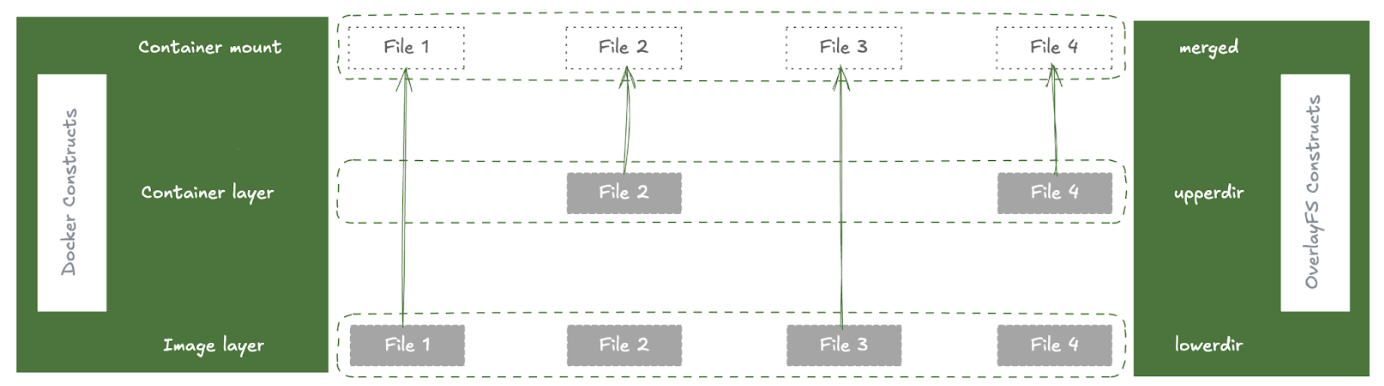
In containerd, a snapshotter is a plugin responsible for managing container filesystems. Its primary job is to take the layers of an image and assemble them into a rootfs for a container. The default snapshotter in containerd is overlayFS, which uses the Linux kernel’s OverlayFS driver to efficiently stack layers. To assemble the rootfs, the overlayFS snapshotter creates a “merged” view of the read-only image layers:
Figure 4. How OverlayFS assembles the container filesystem.
lowerdir: The read-only image layers are used as the lowerdir in OverlayFS. These are the immutable layers from the container image.
upperdir: A new, empty directory is created to be the upperdir. This is the writable layer for the container where any changes are stored.
merged: The merged directory is the unified view of the lowerdir and upperdir. This is what is presented to the container as its rootfs.
When a container reads a file, it’s read from the merged view. When a container writes a file, it’s written to the upperdir using a copy-on-write mechanism. This is an efficient way to manage container filesystems, as it avoids duplicating files and allows for fast container startup.
The problem: Traditional container image pull
To understand the benefits of lazy loading, we first need to understand the traditional container image pull process:
Download layers: The container runtime downloads all layer tarballs that make up the image.
Unpack layers: Each layer is unpacked and extracted onto the host’s disk.
Create snapshot: The snapshotter combines these layers into a single, unified filesystem, known as the container’s rootfs.
Start container: Only after all layers are downloaded and unpacked can the container start.
This process is slow, especially for large images, as the entire image must be present on the host before the container can launch.
The solution: Remote snapshotter
To address the slow startup issue with large images, we use a remote snapshotter solution. A remote snapshotter is a special type of snapshotter that doesn’t require all image data to be locally present. Instead of downloading and unpacking all the layers, it creates a “snapshot” that points to the remote location of the data (like a container registry). The actual file content is then fetched on-demand when the container tries to read a file for the first time.
While a traditional snapshotter like overlayFS uses directories on the local disk as its lowerdir, a remote snapshotter creates a virtual lowerdir that is backed by the remote registry. This is typically done using FUSE (Filesystem in Userspace). The remote snapshotter creates a FUSE filesystem that presents the contents of the remote layer as if it were a local directory. This FUSE mount is then used as the lowerdir for the overlayFS driver. This allows the remote snapshotter to integrate with the existing overlayFS infrastructure while adding the capability of lazy-loading data from a remote source.
There are two main formats that enable remote snapshotters: eStargz and SOCI.
eStargz format
eStargz is a backward-compatible extension of the standard OCI tar.gz layer format. It has several key features that enable lazy loading:
Individually compressed files: Each file within the layer (and even chunks of large files) is compressed individually. This is the key that allows for random access to file contents.
TOC (table of contents): A JSON file named stargz.index.json is located at the end of the layer. This TOC contains metadata for every file, including its name, size, and, most importantly, its offset within the layer blob.
Footer: A small footer at the very end of the layer contains the offset of the TOC, allowing it to be easily located by reading only the last few bytes of the layer.
Chunking and verification: Large files can be broken down into smaller chunks, each with its own entry in the TOC. Each chunk also has a chunkDigest in its TOC entry, allowing for independent verification of each downloaded piece of data.
Prefetch landmark: A special file, .prefetch.landmark, can be placed in the layer to mark the end of “prioritized files”. This allows the snapshotter to intelligently prefetch the most important files for the container’s workload.
The stargz snapshotter uses the eStargz format to enable lazy loading. Here’s how it works:
Mount request: When containerd calls the Mount function, it’s the main entry point for creating a new filesystem for a layer.
Resolve and read TOC: The snapshotter fetches the layer’s footer, then fetches the stargz.index.json TOC from the remote registry. This TOC contains all the file metadata needed to create a virtual filesystem.
Mount FUSE filesystem: With the TOC in memory, the snapshotter creates a virtual filesystem using FUSE. The container can now start, as it has a valid rootfs, even though most of the file content has not been downloaded.
On-demand fetching: When the container performs a file operation like read(), the FUSE filesystem intercepts the call. The snapshotter checks a local disk cache for the requested bytes. If the data is not cached, it issues an HTTP Range request to the container registry to download only the required chunk of the layer.
Remote fetching and caching: The downloaded data is returned to the container and also written to the local cache for subsequent reads.
Prefetching for optimization: After the FUSE filesystem is mounted, a background goroutine begins downloading the prioritized files (up to the .prefetch.landmark) and can also be configured to download the entire rest of the layer in the background.
SOCI is a technology open sourced by AWS that enables containers to launch faster by lazily loading the container image. SOCI works by creating an index (SOCI Index) of the files within an existing container image. SOCI borrows some of the design principles from stargz-snapshotter but takes a different approach:
Separate index: A SOCI index is generated separately from the container image and is stored in the registry as an OCI Artifact, linked back to the container image by OCI Reference Types.
No image conversion: This means that the container images do not need to be converted, image digests do not change, and image signatures remain valid.
Native Bottlerocket support: SOCI is natively supported on Bottlerocket OS.
When using EKS with containerd as the container runtime, you can configure remote snapshotters to enable lazy loading. Here’s how to set them up:
For stargz-snapshotter (eStargz): You need to install the containerd-stargz-grpc service first, then register it as a proxy plugin in containerd’s configuration:
# /etc/containerd/config.toml
[proxy_plugins]
[proxy_plugins.stargz]
type = "snapshot"
address = "/run/containerd-stargz-grpc/containerd-stargz-grpc.sock"
For detailed installation instructions, see the stargz-snapshotter installation documentation. The setup can be baked into an AMI for production use or tested via user data from node bootstrap scripts.
For SOCI snapshotter (Bottlerocket): On Bottlerocket nodes, enable the SOCI snapshotter via user data:
SOCI doesn’t require rebuilding images; you only need to generate a SOCI index for existing images. Since Docker doesn’t natively support SOCI index generation yet, workaround solutions include using the AWS SOCI Index Builder Using Lambda Functions or integrating SOCI index generation into your CI/CD pipeline as described in this blog post.
Key takeaway: Why we chose SOCI
We started our exploration with eStargz but ultimately chose SOCI for production deployment. The key reason is scalability and alignment with our strategy to use Bottlerocket OS for enhancing Kubernetes pod startup and security. SOCI is natively supported by Bottlerocket, which means service teams don’t need to set up and maintain the more complicated stargz snapshotter across all EKS clusters. This makes the implementation easier to maintain and provides better support from AWS.
Additionally, we learned that lazy loading doesn’t eliminate the time required to download image data; it redistributes it from startup time to runtime. While this dramatically improves cold start performance, it’s important to monitor application performance closely and tune configuration parameters based on your workload and infrastructure. We achieved a 60% improvement by optimizing SOCI’s parallel pull mode settings, demonstrating the value of proper configuration tuning.
Conclusion
Docker image lazy loading with SOCI offers a significant opportunity to improve the performance and efficiency of our services at Grab. Our testing and production deployments have shown:
4x faster image pull times on fresh nodes.
29-34% improvement in P95 startup times for production workloads.
60% improvement in image download times with proper configuration tuning.
The implementation path is clear, low-risk, and builds on proven components. This technology is production-ready, and we’re continuing to scale it across more services.
Grab is a leading superapp in Southeast Asia, operating across the deliveries, mobility and digital financial services sectors. Serving over 800 cities in eight Southeast Asian countries, Grab enables millions of people everyday to order food or groceries, send packages, hail a ride or taxi, pay for online purchases or access services such as lending and insurance, all through a single app. Grab was founded in 2012 with the mission to drive Southeast Asia forward by creating economic empowerment for everyone. Grab strives to serve a triple bottom line – we aim to simultaneously deliver financial performance for our shareholders and have a positive social impact, which includes economic empowerment for millions of people in the region, while mitigating our environmental footprint.
Powered by technology and driven by heart, our mission is to drive Southeast Asia forward by creating economic empowerment for everyone. If this mission speaks to you, join our team today!
Konstantin Ryabitsev has put up a
blog post about korgalore, a tool he has written to circumvent delivery
problems experienced by kernel developers using the large, centralized
email systems.
We cannot fix email delivery, but we can sidestep it
entirely. Public-inbox archives like lore.kernel.org store all
mailing list traffic in git repositories. In its simplest
configuration, korgalore can shallow-clone these repositories
directly and upload any new messages straight to your mailbox using
the provider’s API.
Today, we’re announcing the general availability of Amazon Elastic Compute Cloud (Amazon EC2) G7e instances that deliver cost-effective performance for generative AI inference workloads and the highest performance for graphics workloads.
G7e instances are accelerated by the NVIDIA RTX PRO 6000 Blackwell Server Edition GPUs and are well suited for a broad range of GPU-enabled workloads including spatial computing and scientific computing workloads. G7e instances deliver up to 2.3 times inference performance compared to G6e instances.
Improvements made compared to predecessors:
NVIDIA RTX PRO 6000 Blackwell GPUs — NVIDIA RTX PRO 6000 Blackwell Server Edition GPUs offer two times the GPU memory and 1.85 times the GPU memory bandwidth compared to G6e instances. By using the higher GPU memory offered by G7e instances, you can run medium-sized models of up to 70B parameters with FP8 precision on a single GPU.
NVIDIA GPUDirect P2P — For models that are too large to fit into the memory of a single GPU, you can split the model or computations across multiple GPUs. G7e instances reduce the latency of your multi-GPU workloads with support for NVIDIA GPUDirect P2P, which enables direct communication between GPUs over PCIe interconnect. These instances offer the lowest peer to peer latency for GPUs on the same PCIe switch. Additionally, G7e instances offer up to four times the inter-GPU bandwidth compared to L40s GPUs featured in G6e instances, boosting the performance of multi-GPU workloads. These improvements mean you can run inference for larger models across multiple GPUs offering up to 768 GB of GPU memory in a single node.
Networking — G7e instances offer four times the networking bandwidth compared to G6e instances, which means you can use the instance for small-scale multi-node workloads. Additionally, multi-GPU G7e instances support NVIDIA GPUDirect Remote Direct Memory Access (RDMA) with Elastic Fabric Adapter (EFA), which reduces the latency of remote GPU-to-GPU communication for multi-node workloads. These instance sizes also support NVIDIA GPUDirectStorage with Amazon FSx for Lustre, which increases throughput by up to 1.2 Tbps to the instances compared to G6e instances, which means you can quickly load your models.
EC2 G7e specifications G7e instances feature up to 8 NVIDIA RTX PRO 6000 Blackwell Server Edition GPUs with up to 768 GB of total GPU memory (96 GB of memory per GPU) and Intel Emerald Rapids processors. They also support up to 192 vCPUs, up to 1,600 Gbps of network bandwidth, up to 2,048 GiB of system memory, and up to 15.2 TB of local NVMe SSD storage.
Now available Amazon EC2 G7e instances are available today in the US East (N. Virginia) and US East (Ohio) AWS Regions. For Regional availability and a future roadmap, search the instance type in the CloudFormation resources tab of AWS Capabilities by Region.
One would assume that most LWN readers stopped running network-accessible
telnet services some number of decades ago. For the rest of you, this security advisory from
Simon Josefsson is worthy of note:
The telnetd server invokes /usr/bin/login (normally running as
root) passing the value of the USER environment variable received
from the client as the last parameter.
If the client supplies a carefully crafted USER environment value
being the string “-f root”, and passes the telnet(1) -a or –login
parameter to send this USER environment to the server, the client
will be automatically logged in as root bypassing normal
authentication processes.
This is a guest post by Oleh Khoruzhenko, Senior Staff DevOps Engineer at Bazaarvoice, in partnership with AWS.
Bazaarvoice is an Austin-based company powering a world-leading reviews and ratings platform. Our system processes billions of consumer interactions through ratings, reviews, images, and videos, helping brands and retailers build shopper confidence and drive sales by using authentic user-generated content (UGC) across the customer journey. The Bazaarvoice Trust Mark is the gold standard in authenticity.
Apache Kafka is one of the core components of our infrastructure, enabling real-time data streaming for the global review platform. Although Kafka’s distributed architecture met our needs for high-throughput, fault-tolerant streaming, self-managing this complex system diverted critical engineering resources away from our core product development. Each component of our Kafka infrastructure required specialized expertise, ranging from configuring low-level parameters to maintaining the complex distributed systems that our customers rely on. The dynamic nature of our environment demanded continuous care and investment in automation. We found ourselves constantly managing upgrades, applying security patches, implementing fixes, and addressing scaling needs as our data volumes grew.
In this post, we show you the steps we took to migrate our workloads from self-hosted Kafka to Amazon Managed Streaming for Apache Kafka (Amazon MSK). We walk you through our migration process and highlight the improvements we achieved after this transition. We show how we minimized operational overhead, enhanced our security and compliance posture, automated key processes, and built a more resilient platform while maintaining the high performance our global customer base expects.
The need for modernization
As our platform grew to process billions of daily consumer interactions, we needed to find a way to scale our Kafka clusters efficiently while maintaining a small team to manage the infrastructure. The limitations of self-managed Kafka clusters manifested in several key areas:
Scaling operations – Although scaling our self-hosted Kafka clusters wasn’t inherently complex, it required careful planning and execution. Each time we needed to add new brokers to handle increased workload, our team faced a multi-step process involving capacity planning, infrastructure provisioning, and configuration updates.
Configuration complexity – Kafka offers hundreds of configuration parameters. Although we didn’t actively manage all of these, understanding their impact was important. Key settings like I/O threads, memory buffers, and retention policies needed ongoing attention as we scaled. Even minor adjustments could have significant downstream effects, requiring our team to maintain deep expertise in these parameters and their interactions to ensure optimal performance and stability.
Infrastructure management and capacity planning – Self-hosting Kafka required us to manage multiple scaling dimensions, including compute, memory, network throughput, storage throughput, and storage volume. We needed to carefully plan capacity for all these components, often making complex trade-offs. Beyond capacity planning, we were responsible for real-time management of our Kafka infrastructure. This included promptly detecting and addressing component failures and performance issues. Our team needed to be highly responsive to alerts, often requiring immediate action to maintain system stability.
Specialized expertise requirements – Operating Kafka at scale demanded deep technical expertise across multiple domains. The team needed to:
Monitor and analyze hundreds of performance metrics
Conduct complex root cause analysis for performance issues
Manage ZooKeeper ensemble coordination
Execute rolling updates for zero-downtime upgrades and security patches
These challenges were compounded during peak business periods, such as Black Friday and Cyber Monday, when maintaining optimal performance was essential for Bazaarvoice’s retail customers.
Choosing Amazon MSK
After evaluating various options, we selected Amazon MSK as our modernization solution. The decision was driven by the service’s ability to minimize operational overhead, provide high availability out of the box with its three Availability Zone architecture, and offer seamless integration with our existing AWS infrastructure.
Key capabilities that made Amazon MSK the clear choice:
AWS integration – We already used AWS services for data processing and analytics. Amazon MSK connected directly with these services, alleviating the need to build and maintain custom integrations. This meant our existing data pipelines would continue working with minimal changes.
Automated operations management – Amazon MSK automated our most time-consuming tasks. We no longer need to manually monitor instances and storage for failures or respond to these issues ourselves.
Enterprise-grade reliability – The platform’s architecture matched our reliability requirements out of the box. Multi-AZ distribution and built-in replication gave us the same fault tolerance we’d carefully built into our self-hosted system, now backed by AWS’s service guarantees.
Simplified upgrade process – Before Amazon MSK, version upgrades for our Kafka clusters required careful planning and execution. The process was complex, involving multiple steps and risks. Amazon MSK simplified our upgrade operations. We now use automated upgrades for dev and test workloads and maintain control over production environments. This shift reduced the need for extensive planning sessions and multiple engineers. As a result, we stay current with the latest Kafka versions and security patches, improving our system reliability and performance.
Enhanced security controls – Our platform required ISO 27001 compliance, which typically involved months of documentation and security controls implementation. Amazon MSK came with this certification built-in, alleviating the need for separate compliance work. Amazon MSK encrypted our data, controlled network access, and integrated with our existing security tools.
With Amazon MSK selected as our target platform, we began planning the complex task of migrating our critical streaming infrastructure without disrupting the billions of consumer interactions flowing through our system.
Bazaarvoice’s migration journey
Moving our complex Kafka infrastructure to Amazon MSK required careful planning and precise execution. Our platform processes data through two main components: an Apache Kafka Streams pipeline that handles data processing and augmentation, and client applications that move this enriched data to downstream systems. With 40 TB of state across 250 internal topics, this migration demanded a methodical approach.
Planning phase
Working with AWS Solutions Architects proved critical for validating our migration strategy. Our platform’s unique characteristics required special consideration:
Multi-Region deployment across the US and EU
Complex stateful applications with strict data consistency needs
Vital business services requiring zero downtime
Diverse consumer ecosystem with different migration requirements
Migration challenges
The biggest hurdle was migrating our stateful Kafka Streams applications. Our data processing runs as a directed acyclic graph (DAG) of applications across regions, using static group membership to prevent disruptive rebalancing. It’s important to note that Kafka Streams keeps its state in internal Kafka topics. For applications to recover properly, replicating this state accurately is crucial. This characteristic of Kafka Streams added complexity to our migration process. Initially, we considered MirrorMaker2, the standard tool for Kafka migrations. However, two fundamental limitations made it challenging:
Risk of losing state or incorrectly replicating state across our applications.
Inability to run two instances of our applications simultaneously, which meant we needed to shut down the main application and wait for it to recover from the state in the MSK cluster. Given the size of our state, this recovery process exceeded our 30-minute SLA for downtime.
Our solution
We decided to deploy a parallel stack of Kafka Streams applications reading and writing data from Amazon MSK. This approach gave us sufficient time for testing and verification, and enabled the applications to hydrate their state before we delivered the output to our data warehouse for analytics. We used MirrorMaker2 for input topic replication, while our solution offered several advantages:
Simplified monitoring of the replication process
Avoided consistency issues between state stores and internal topics
Allowed for gradual, controlled migration of consumers
Enabled thorough validation before cutover
Required a coordinated transition plan for all consumers, because we couldn’t transfer consumer offsets across clusters
Consumer migration strategy
Each consumer type required a carefully tailored approach:
Standard consumers – For applications supporting Kafka Consumer Group protocol, we implemented a four-step migration. This approach risked some duplicate processing, but our applications were designed to handle this scenario. The steps were as follows:
Configure consumers with auto.offset.reset: latest.
Stop all DAG producers.
Wait for existing consumers to process remaining messages.
Cut over consumer applications to Amazon MSK.
Apache Kafka Connect Sinks – Our sink connectors served two critical databases:
A distributed search and analytics engine – Document versioning depended on Kafka record offsets, making direct migration impossible. To address this, we implemented a solution that involved building new search engine clusters from scratch.
A document-oriented NoSQL database – This supported direct migration without requiring new database instances, simplifying the process significantly.
Apache Spark and Flink applications – These presented unique challenges due to their internal checkpointing mechanisms:
Offsets managed outside Kafka’s consumer groups
Checkpoints incompatible between source and target clusters
Required complete data reprocessing from the beginning
We scheduled these migrations during off-peak hours to minimize impact.
Technical benefits and improvements
Moving to Amazon MSK fundamentally changed how we manage our Kafka infrastructure. The transformation is best illustrated by comparing key operational tasks before and after the migration, summarized in the following table.
Activity
Before: Self-Hosted Kafka
After: Amazon MSK
Security patching
Required dedicated team time for Kafka and OS updates
Fully automated
Broker recovery
Needed manual monitoring and intervention
Fully automated
Client authentication
Complex password rotation procedures
AWS Identity and Access Management (IAM)
Version upgrades
Complex procedure requiring extensive planning
Fully automated
The details of the tasks are as follows:
Security patching – Previously, our team spent 8 hours monthly applying Kafka and operating system (OS) security patches across our broker fleet. Amazon MSK now handles these updates automatically, maintaining our security posture without engineering intervention.
Broker recovery – Although our self-hosted Kafka had automatic recovery capabilities, each incident required careful monitoring and occasional manual intervention. With Amazon MSK, node failures and storage degradation issues such as Amazon Elastic Block Store (Amazon EBS) slowdowns are handled entirely by AWS and resolved within minutes without our involvement.
Authentication management – Our self-hosted implementation required password rotations for SASL/SCRAM authentication, a process that took two engineers several days to coordinate. The direct integration between Amazon MSK and AWS Identity and Access Management (IAM) minimized this overhead while strengthening our security controls.
Version upgrades – Kafka version upgrades in our self-hosted environment required weeks of planning and testing as well as weekend maintenance windows. Amazon MSK manages these upgrades automatically during off-peak hours, maintaining our SLAs without disruption.
These improvements proved especially valuable during high-traffic periods like Black Friday, when our team previously needed extensive operational readiness plans. Now, the built-in resiliency of Amazon MSK provides us with reliable Kafka clusters that serve as mission-critical infrastructure for our business. The migration made it possible to break our monolithic clusters into smaller, dedicated MSK clusters. This improved our data isolation, provided better resource allocation, and enhanced performance predictability for high-priority workloads.
Lessons learned
Our migration to Amazon MSK revealed several key insights that can help other organizations modernize their Kafka infrastructure:
Expert validation – Working with AWS Solutions Architects to validate our migration strategy caught several critical issues early. Although our team knew our applications well, external Kafka experts identified potential problems with state management and consumer offset handling that we hadn’t considered. This validation prevented costly missteps during the migration.
Data verification – Comparing data across Kafka clusters proved challenging. We built tools to capture topic snapshots in Parquet format on Amazon Simple Storage Service (Amazon S3), enabling quick comparisons using Amazon Athena queries. This approach gave us confidence that data remained consistent throughout the migration.
Start small – Beginning with our smallest data universe in QA helped us refine our process. Each subsequent migration went smoother as we applied lessons from previous iterations. This gradual approach helped us maintain system stability while building team confidence.
Detailed planning – We created specific migration plans with each team, considering their unique requirements and constraints. For example, our machine learning pipeline needed special handling due to strict offset management requirements. This granular planning prevented downstream disruptions.
Performance optimization – We found that utilizing Amazon MSK provisioned throughput offered clear cost advantages when storage throughput became a bottleneck. This feature made it possible to improve cluster performance without scaling instance sizes or adding brokers, providing a more efficient solution to our throughput challenges.
Documentation – Maintaining detailed migration runbooks proved invaluable. When we encountered similar issues across different migrations, having documented solutions saved significant troubleshooting time.
Conclusion
In this post, we showed you how we modernized our Kafka infrastructure by migrating to Amazon MSK. We walked through our decision-making process, challenges faced, and strategies employed. Our journey transformed Kafka operations from a resource-intensive, self-managed infrastructure to a streamlined, managed service, improving operational efficiency, platform reliability, and team productivity. For enterprises managing self-hosted Kafka infrastructure, our experience demonstrates that successful transformation is achievable with proper planning and execution. As data streaming needs grow, modernizing infrastructure becomes a strategic imperative for maintaining competitive advantage.
For more information, visit the Amazon MSK product page, and explore the comprehensive Developer Guide to learn about the features available to help you build scalable and reliable streaming data applications on AWS.
Organizations managing large-scale analytical workloads increasingly face challenges with traditional Apache Parquet-based data lakes with Hive-style partitioning, including slow queries, complex file management, and limited consistency guarantees. Apache Iceberg addresses these pain points by providing ACID transactions, seamless schema evolution, and point-in-time data recovery capabilities that transform how enterprises handle their data infrastructure.
In this post, we demonstrate how you can achieve migration at scale from existing Parquet tables to Apache Iceberg tables. Using Amazon DynamoDB as a central orchestration mechanism, we show how you can implement in-place migrations that are highly configurable, repeatable, and fault-tolerant—unlocking the full potential of modern data lake architectures without extensive data movement or duplication.
Solution overview
When performing in-place migration, Apache Iceberg uses its ability to directly reference existing data files. This capability is only supported for formats such as Parquet, ORC, and Avro, because these formats are self-describing and include consistent schema and metadata information. Unlike raw formats such as CSV or JSON, they enforce structure and support efficient columnar or row-based access, which allows Iceberg to integrate them without rewriting the data.
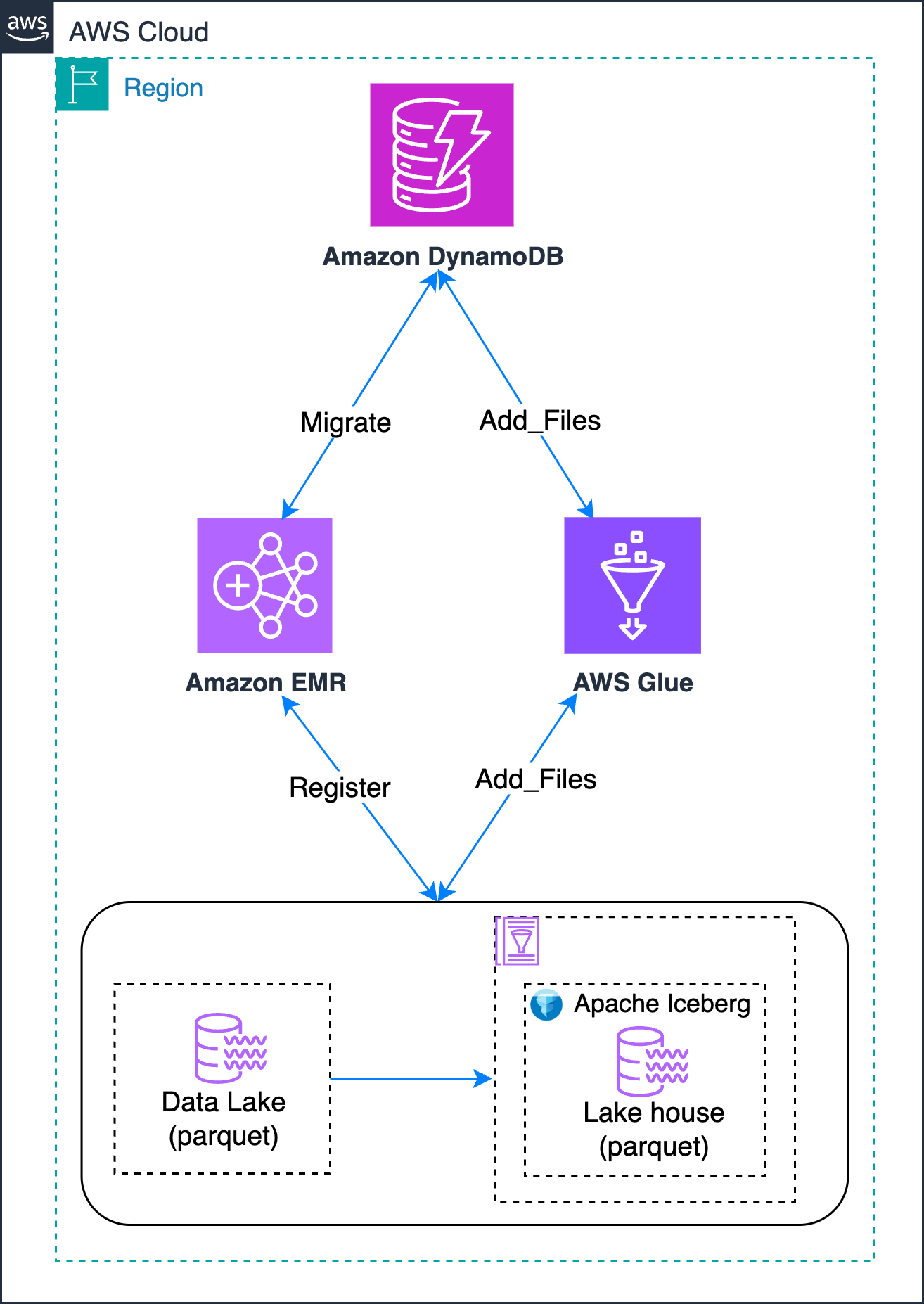
In this post, we demonstrate how you can migrate an existing Parquet-based data lake that isn’t cataloged in AWS Glue by using two methodologies:
Apache Iceberg migrate and register_table approach. Ideal for converting existing Hive-registered Parquet tables into Iceberg-managed tables.
Iceberg add_files approach. Best suited for quickly onboarding raw Parquet data into Iceberg without rewriting files.
The solution also incorporates a DynamoDB table that acts as a scalable control plane, so you can perform in-place migration of your data lake from Parquet format to Iceberg format.
The following diagram shows different methodologies that you can use to achieve this in-place migration of your Hive-style partitioned data lake:
You use DynamoDB to track the migration state, handling retries and recording errors and outcomes. This provides the following benefits:
An Amazon EMR cluster using Hive as the metastore, with SSH access. (See Appendix A for setup instructions.)
An Amazon EMR cluster or Amazon EMR Serverless environment using AWS Glue Data Catalog as the Spark metastore, with SSH access. (See Appendix B for setup instructions.)
For AWS Glue exchange, transform, and load (ETL), use Glue 4.0 or later.
Create sample Parquet dataset as a source
You can create the sample Parquet dataset for testing the different methodologies using the Athena query editor. Replace <amzn-s3-demo-bucket> with an available bucket in your account.
Create an AWS Glue database(test_db), if not present.
CREATE DATABASE IF NOT EXISTS test_db
Create a sample Parquet table (table1) and add to be used for testing the add_files approach.
CREATE TABLE table1
WITH (
  external_location = 's3://<amzn-s3-demo-bucket>/table1/',
  format = 'PARQUET',
  partitioned_by = ARRAY['date', 'hour']
)
AS
SELECT
  1 as id,
  'John Doe' as name,
  25 as age,
  'Engineer' as job_title,
  current_date as created_date,
  current_date as date,
  hour(current_timestamp) as hour
UNION ALL
SELECT 2, 'Jane Smith', 30, 'Manager', current_date, current_date, hour(current_timestamp)
UNION ALL
SELECT 3, 'Bob Johnson', 35, 'Analyst', current_date, current_date, hour(current_timestamp);
Create a sample Parquet table (table2) and add data to be used for testing the migrate and register_table approach. Replace <amzn-s3-demo-bucket> with your bucket name.
CREATE TABLE table2
WITH (
  external_location = 's3://<amzn-s3-demo-bucket>/table2/',
  format = 'PARQUET',
  partitioned_by = ARRAY['date', 'hour']
)
AS
SELECT
  1 as id,
  'John Doe' as name,
  25 as age,
  'Engineer' as job_title,
  current_date as created_date,
  current_date as date,
  hour(current_timestamp) as hour
UNION ALL
SELECT 2, 'Jane Smith', 30, 'Manager', current_date, current_date, hour(current_timestamp)
UNION ALL
SELECT 3, 'Bob Johnson', 35, 'Analyst', current_date, current_date, hour(current_timestamp);
Drop the tables from the Data Catalog because you only need Parquet data with the Hive-style partitioning structure.
DROP TABLE IF EXISTS test_db.table1
Create a DynamoDB control table
Before beginning the migration process, you must create a DynamoDB table that serves as the control plane. This table maps source Amazon S3 paths to their corresponding Iceberg database and table destinations, enabling systematic tracking of the migration process.
To implement this control mechanism, create a table with the following structure:
A primary key s3_path that stores the source Parquet data location
Two attributes that define the target Iceberg location:
target_db_name
target_table_name
To create the DynamoDB control table
Create the Amazon DynamoDB table using the following AWS CLI command:
In this section, you explore two methodologies for migrating your existing Parquet tables to Apache Iceberg format:
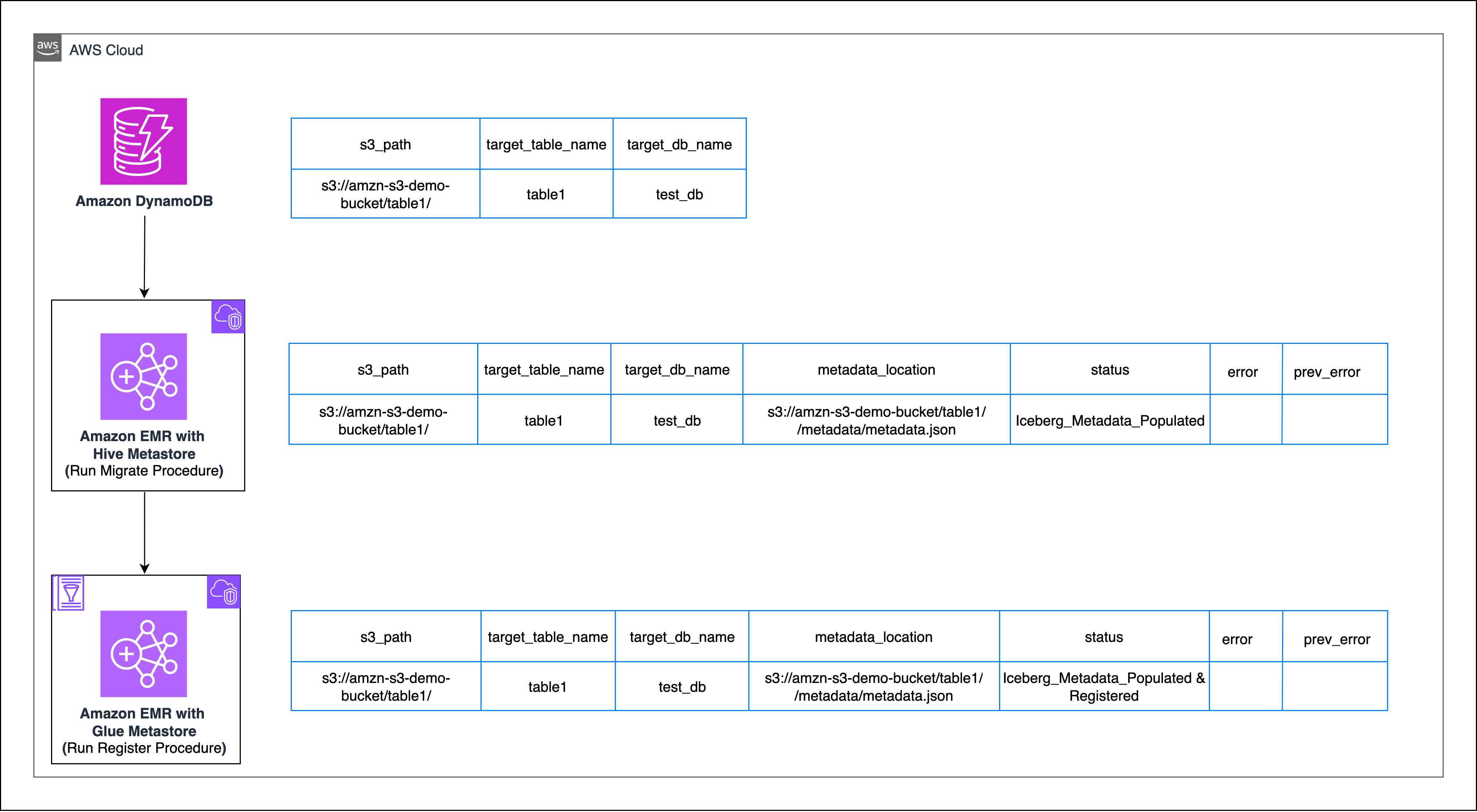
Apache Iceberg migrate and register_table approach – This approach first converts your Parquet table to Iceberg format using the native migrate procedure, followed by registering it in AWS Glue using the register_table procedure.
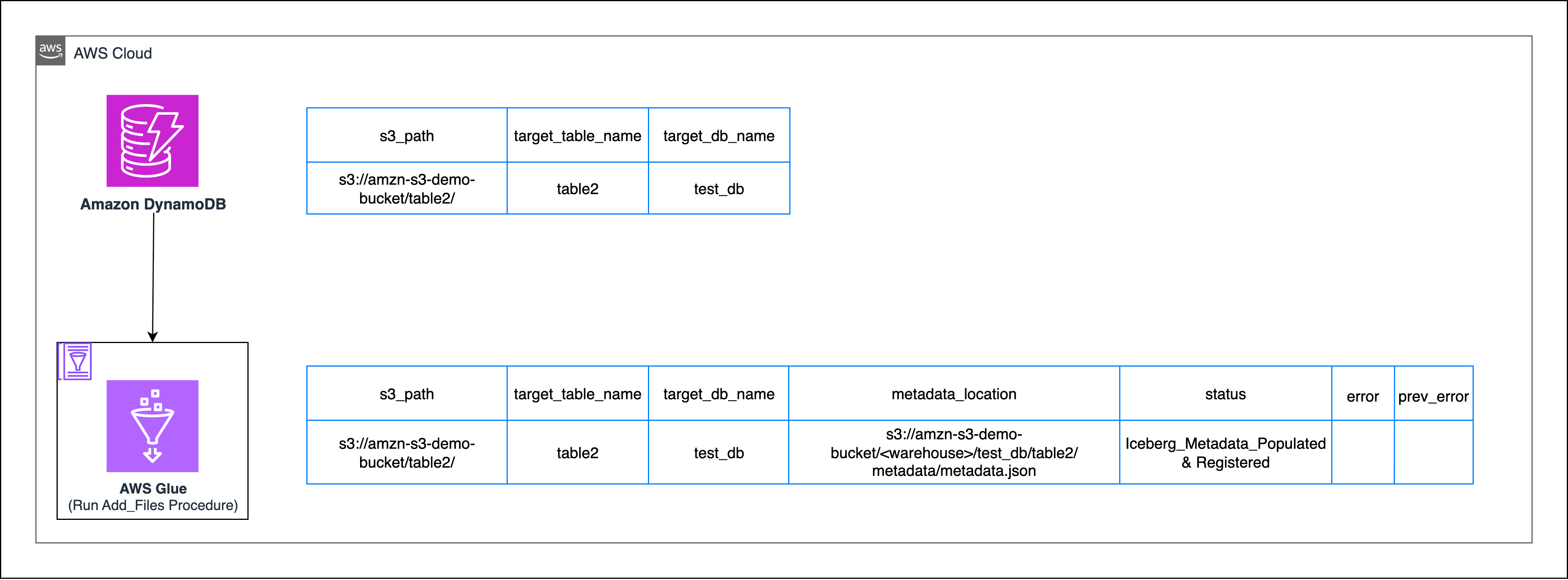
Apache Iceberg add_files approach – This method creates an empty Iceberg table and uses the add_files procedure to import existing Parquet data files without physically moving them.
Apache Iceberg migrate and register_table procedure
Use the Apache Iceberg Migrate procedure that is used for in-place conversion of an existing Hive or Parquet table into an Iceberg-managed table. Thereafter, you can use the Apache Iceberg RegisterTable procedure to register the respective table in AWS Glue.
Migrate
In your EMR cluster with Hive as the metastore, create a PySpark session with the following Iceberg Packages:
This post uses Iceberg v1.9.1 (Amazon EMR build), which is native to Amazon EMR 7.11. Always verify the latest supported version and update package coordinates accordingly.
Next, create your corresponding table in your Hive catalog (you can skip this step if you already have tables created in your hive catalog). Replace <amzn-s3-demo-bucket> with the name of your S3 bucket. In the following snippet, change or remove the PARTITIONED BY command based on the partition strategy of your table, the MSCK Repair table command should only be run if your respective table is partitioned.
#You can automate this for production Scaling with DynamoDB as control table
s3_path = "s3://<amzn-s3-demo-bucket>/table1/"
target_db_name = "test_db"
target_table_name = "table1"
# Read data in a dataframe to infer schema
df = spark.read.parquet(s3_path)
df.createOrReplaceTempView("temp_view")
# Get schema as string
schema = spark.table("temp_view").schema
schema_string = ", ".join([f"{field.name} {field.dataType.simpleString()}" for field in schema])
# Create Database If not exists
spark.sql(f"CREATE DATABASE IF NOT EXISTS {target_db_name}").show()
# full_table_name= test_db.table1
full_table_name = f"{target_db_name}.{target_table_name}"
# Create table
spark.sql(f"""
CREATE TABLE IF NOT EXISTS {full_table_name} (
    {schema_string}
)
STORED AS PARQUET
PARTITIONED BY (date, hour)
LOCATION '{s3_path}'
""")
# Refresh, repair, and validate
spark.sql(f"REFRESH TABLE {full_table_name}")
spark.sql(f"MSCK REPAIR TABLE {full_table_name}")
Convert the Parquet table to an Iceberg table in Hive
# Run migration procedure
spark.sql(f"CALL spark_catalog.system.migrate('{full_table_name}')")
# Validate that the table is successfully migrated
spark.sql(f"DESCRIBE FORMATTED {full_table_name}").show(truncate=False)
Run the migrate command to convert the Parquet-based table to an Iceberg table, creating the metadata folder and the metadata.json file therein
You can stop at this point if you don’t intend to migrate your existing iceberg table from Hive to the Data Catalog.
Register
Sign in to the AWS Glue as Spark Catalog enabled EMR cluster.
Register the Iceberg table to your Data Catalog.
Create the session with the respective Iceberg Packages. Replace <amzn-s3-demo-bucket> with your bucket name, and <warehouse> with warehouse directory.
Run the register_table command to make the Iceberg table visible in AWS Glue.
register_table registers an existing Iceberg table’s metadata file (metadata.json) with a catalog(glue_catalog) so that Spark (and other engines) can query it.
The procedure creates a Data Catalog entry for the table, pointing it to the given metadata location.
Replace <amzn-s3-demo-bucket> and <metadata-prefix> with the name of your S3 bucket and metadata prefix name.
Ensure that your EMR Spark Cluster has been configured with appropriate AWS Glue permissions
# You can automate this for production Scaling with DynamoDB as control table
metadata_location = "s3://<amzn-s3-demo-bucket>/table1/metadata/<metadata-prefix>.metadata.json"
target_db_name = "test_db"
target_table_name = "table1"
full_table_name = f"{target_db_name}.{target_table_name}"
# Register existing Iceberg table metadata in Glue Catalog
spark.sql(f"CALL glue_catalog.system.register_table('{full_table_name}', '{metadata_location}')")
# Set table properties (example: Iceberg format version 2)
spark.sql(f"ALTER TABLE glue_catalog.{full_table_name} SET TBLPROPERTIES('format-version'='2')")
Validate that the Iceberg table is now visible in the Data Catalog.
# Lookout for format as iceberg/parquet
spark.sql("SHOW TBLPROPERTIES glue_catalog.test_db.table1").show()
Apache Iceberg’s add_files procedure
Here, you’re going to use Iceberg’s add_files procedure to import raw data files (Parquet, ORC, Avro) into an existing Iceberg table by updating its metadata. This procedure works for both Hive and Data Catalog, it doesn’t physically move or rewrite the files—it only registers them so Iceberg can manage them.
This methodology comprises the following steps:
Create an empty Iceberg table in AWS Glue. Because the add_files procedure expects the iceberg table to be already present, you need to create an empty Iceberg table by inferring the table schema.
Register existing data locations to the Iceberg table
Using the add_files procedure in a Glue-backed Iceberg catalog will register the target S3 path along with all its subdirectories to the empty Iceberg table created in the previous step.
You can consolidate both steps into a single Spark job. For the following AWS Glue job, you have specified iceberg as a value for the --datalake-formats job parameter. See the AWS Glue job configuration documentation for more details.
Replace <amzn-s3-demo-bucket> with your S3 bucket name and <warehouse> with warehouse directory.
When working with non-Hive partitioned datasets, a direct migration to Apache Iceberg using add_files might not behave as expected. See Appendix C for more information.
Considerations
Let’s explore two key considerations that you should address when implementing your migration strategy.
State management using DynamoDB control table
Use the following sample code snippet to update the state of DynamoDB table:
This ensures that any errors are logged and saved to DynamoDB as error_message. On successive retries, previous errors move to prev_error_message and new errors overwrite error_message. Successful operations clear error_message and archive the last error.
Protecting your data from unintended deletion
To protect your data from unintended deletion, never delete data or metadata files from Amazon S3 directly. Iceberg tables that are registered in AWS Glue or Athena are managed tables and should be deleted using the DROP TABLE command from Spark or Athena. The DROP TABLE command deletes both the table metadata and the underlying data files in S3. See Appendix D for more information.
Clean up
Complete the following steps to clean up your resources:
Delete the EMR clusters and AWS Glue job used for testing
Conclusion
In this post, we showed you how to modernize your Parquet-based data lake into an Apache Iceberg–powered lakehouse without rewriting or duplicating data. You learned two complementary approaches for this in-place migration:
Migrate and register – Ideal for converting existing Hive-registered Parquet tables into Iceberg-managed tables.
add_files – Best suited for quickly onboarding raw Parquet data into Iceberg without rewriting files.
Both approaches benefit from DynamoDB centralized state tracking, which enables retries, error auditing, and lifecycle management across multiple datasets.
By combining Apache Iceberg with Amazon EMR, AWS Glue, and Amazon DynamoDB, you can create a production-ready migration pipeline that is observable, automated, and straightforward to extend to future data format upgrades. This pattern forms a solid foundation for building an Iceberg-based lakehouse on AWS, helping you achieve faster analytics, better data governance, and long-term flexibility for evolving workloads.
To get started, try implementing this solution using the sample tables (table1 and table2) that you created using Athena queries. we encourage you to share your migration experiences and questions in the comments.
Appendix A — Creating an EMR cluster for Hive metastore using console and AWS CLI
Console steps:
Open AWS Management Console for Amazon EMR and choose Create cluster.
Select Spark or Hive under applications.
Under AWS Glue Data Catalog settings, make sure the following options are not selected:
Appendix C — Non-Hive partitioned datasets and Iceberg add_files
This appendix explains why a direct in-place migration using an add_files-style procedure might not behave as expected for datasets that aren’t Hive-partitioned and shows recommended fixes and examples.
AWS Glue and Athena follow Hive-style partitioning, where partition column values are encoded in the S3 path rather than inside the data files. For example, following the Parquet dataset created in the Create Sample Parquet Dataset as a source section of this post:
If you try to create an empty Iceberg table and directly load it using add_files on a non-hive layout, the following happens:
Iceberg cannot automatically map partitions, add_files operations fail or register files with incorrect or missing partition metadata.
Queries in Athena or AWS Glue will return unexpected NULLs or incomplete results.
Successive incremental writes using add_files will fail.
Recommended approaches:
Create an AWS Glue table and use the Iceberg snapshot procedure:
Create a table in AWS Glue pointing to your existing Parquet dataset.
You might need to manually provide the schema because glue crawler might fail to automatically infer it for you.
Use Iceberg’ s snapshot procedure to convert and move the AWS Glue table into your target Iceberg table.
This works because Iceberg relies on AWS Glue for schema inference, so this approach ensures correct mapping of columns and partitions without rewriting the data. For more information, see Snapshot procedure.
Appendix D — Understanding table types: Managed compared to external
By default, all non-Iceberg tables created in AWS Glue or Athena are external tables, Athena doesn’t manage the underlying data. If you use CREATE TABLE without the EXTERNAL keyword for non-Iceberg tables, Athena issues an error.
However, when dealing with Iceberg tables, AWS Glue and Athena also manage the underlying data for the respective tables, so these tables are treated as internal tables.
Running DROP TABLE on Iceberg tables will delete the table and the underlying data.
The following table describes how the effect of DELETE and DROP TABLE actions on Iceberg tables in AWS Glue and Athena:
Operation
What it does
Effect on S3 data
DELETE FROM mydb.products_iceberg WHERE date = 2025-10-06;
Amazon Web Services (AWS) is pleased to announce that the Fall 2025 System and Organization Controls (SOC) 1, 2, and 3 reports are now available. The reports cover 185 services over the 12-month period from October 1, 2024–September 30, 2025, giving customers a full year of assurance. These reports demonstrate our continuous commitment to adhering to the heightened expectations of cloud service providers.
AWS strives to continuously bring services into the scope of its compliance programs to help customers meet their architectural and regulatory needs. You can view the current list of services in scope on our Services in Scope page. As an AWS customer, you can reach out to your AWS account team if you have any questions or feedback about SOC compliance.
To learn more about AWS compliance and security programs, see AWS Compliance Programs. As always, we value feedback and questions; reach out to the AWS Compliance team through the Contact Us page.
If you have feedback about this post, submit comments in the Comments section below.
The collective thoughts of the interwebz
Manage Consent
To provide the best experiences, we use technologies like cookies to store and/or access device information. Consenting to these technologies will allow us to process data such as browsing behavior or unique IDs on this site. Not consenting or withdrawing consent, may adversely affect certain features and functions.
Functional
Always active
The technical storage or access is strictly necessary for the legitimate purpose of enabling the use of a specific service explicitly requested by the subscriber or user, or for the sole purpose of carrying out the transmission of a communication over an electronic communications network.
Preferences
The technical storage or access is necessary for the legitimate purpose of storing preferences that are not requested by the subscriber or user.
Statistics
The technical storage or access that is used exclusively for statistical purposes.The technical storage or access that is used exclusively for anonymous statistical purposes. Without a subpoena, voluntary compliance on the part of your Internet Service Provider, or additional records from a third party, information stored or retrieved for this purpose alone cannot usually be used to identify you.
Marketing
The technical storage or access is required to create user profiles to send advertising, or to track the user on a website or across several websites for similar marketing purposes.