Post Syndicated from The Hook Up original https://www.youtube.com/watch?v=OyL2ZeJRSGo
Trump’s DOJ & Grand Jury Indictments #lastweektonight
Post Syndicated from LastWeekTonight original https://www.youtube.com/shorts/zrdvWsjhwM0
Security updates for Friday
Post Syndicated from jzb original https://lwn.net/Articles/1088919/
Security updates have been issued by AlmaLinux (.NET 10.0, .NET 8.0, .NET 9.0, bind, bind9.16, and dracut), Debian (apr-util, chromium, postgresql-17, python-httplib2, unzip, and zip), Fedora (erlang-cowboy, erlang-cowlib, flatpak, and libnfs), Gentoo (Apache HTTPD, Bubblewrap, Dnsmasq, Exim, Flatpak, libinput, and rsync), Mageia (dhcpcd, qemu, and roundcubemail), Oracle (.NET 8.0, .NET 9.0, bind, bind9.16, freerdp, glib2, gnome-remote-desktop, grafana, gstreamer1-plugins-good, isns-utils, java-17-openjdk, kernel, libpng, libXfont2, nghttp2, perl-DBI:1.641, python-idna, python3.9, and xorg-x11-server), Slackware (rsync), SUSE (bouncycastle, chromium, dnsdist, dracut, java-1_8_0-ibm, kernel, libXfont2, nodejs22, nodejs24, php8, python-httplib2, rrdtool, rsyslog, samba, and wireshark), and Ubuntu (linux, linux-aws, linux-kvm, linux-aws-hwe, linux-aws-hwe, linux-azure, linux-gcp, linux-hwe, linux-azure, linux-gcp, linux-hwe, linux-oracle, linux-lowlatency, linux-lowlatency-hwe-6.8, linux-nvidia-tegra,
linux-oracle, linux-nvidia-tegra-igx, linux-oem-7.0, linux-oracle, and node-axios).
How Cloudflare detects MCP traffic and helps secure it
Post Syndicated from AJ Gerstenhaber original https://blog.cloudflare.com/mcp-security-updates/
Most companies designed their resource permissions with a human user in mind. A senior engineer may be able to deploy to production, query a sensitive database, or revoke another user's access. Those privileges come with risk, but that risk has traditionally been bounded by two assumptions: the engineer will use human judgment, and the engineer can only act at human speed.
An engineer who sees an unexpected result will usually stop and reconsider their actions. Any human being can only click, type, and review so much in a single day. The introduction of AI agents changes both thresholds. Their decisions are nondeterministic, and they can take the same action (or invoke the same tool) indefinitely, without getting tired or stopping for lunch. A plausible — but incorrect — decision can become thousands of incorrect actions before a human notices.
Today, we're announcing new Cloudflare One capabilities to identify inspected MCP traffic, show which users and servers are generating it, and control direct connections on managed network paths. Combined with MCP Server Portals, these controls help administrators see whether agents are using an approved path, or somehow bypassing it.
Model Context Protocol (MCP) servers give agents a common way to discover and invoke tools backed by third-party SaaS products, internal applications, and APIs. The underlying permissions are likely familiar; what changes is who makes each decision, and how quickly a bad decision can spread.
Connecting an agent to one of these tools can take a single line of configuration. An employee can point Claude Code, Codex, Cursor, OpenCode, VS Code, or any AI harness at an MCP server without checking whether it is approved. The resulting traffic has no obvious shape. The Model Context Protocol does not use a guaranteed hostname or require /mcp in the path, so a direct connection can look like any other HTTPS API call.
To explain how these controls fit together, we'll start with the anatomy of a tool call and the information it exposes. We'll then compare the three places a security team can act: inside the client, on the network, and at the MCP server. From there, we'll show how Cloudflare Gateway uses protocol signals to find shadow MCP traffic and enforce MCP Portal-only access to trusted MCP servers.
The anatomy of an MCP tool call
The same MCP tool call has three forms as it moves through a system. Inside the client it is a decision to invoke a tool with a set of arguments. On the network it is an HTTP transaction carrying a JSON-RPC message. At the server it becomes a call to a tool handler that may read data, change state, or complete some other action.
Consider an agent that wants to know the weather in Austin. A remote MCP request can look like this:
There are several useful signals packed into this request. The hostname and path identify the destination. The authorization header carries the credential used to authenticate the caller when the server requires one. The header: MCP-Protocol-Version identifies the protocol version, while Mcp-Method and Mcp-Name expose the operation and tool in the new stateless protocol. The JSON-RPC envelope repeats the method, gives the request an id that the client can match with a response, and carries the tool arguments in params.
The arguments are the most sensitive part. They can contain a search query, source code, customer data, or instructions for an action such as creating a ticket or changing infrastructure. The tool name says what the agent intends to call; the arguments say what data it will send and what action it wants the server to perform.
If the call succeeds, the server returns a JSON-RPC response with the same id and the tool result. That response may also contain sensitive data. Request inspection can stop an unsafe action before execution, while response inspection and logging show what the tool returned to the agent.
Three places to control an MCP request
The request gives security teams three places to observe or control the call.
Inside the MCP client
A client hook can run after the model selects a tool but before the client serializes the request. From there, it can see the destination server, tool name, and arguments without decrypting network traffic.
This is the earliest stage in the request chain to exercise control. The client can deny a server that is not on an allowlist, ask the user to confirm a sensitive operation, or remove data from the arguments before it leaves the device. It can also cover local stdio (aka local) MCP servers, which never generate network traffic.
This presents a standardization challenge. In order for a security team to benefit from this, they would need to reproduce their controls across every client that their employees use. Client-side controls work best when the organization manages both the client and the device, but telemetry from one client is never a complete inventory of MCP use.
At the device's network boundary
A secure web gateway can observe the HTTP request after it leaves the client. With TLS decryption, it can associate the request with a user and device, inspect the destination and protocol headers, and apply policy without depending on a particular MCP client.
The network layer has the widest lens to detect remote MCP traffic on managed paths. It can identify direct connections to servers outside an approved Portal and block them before the request reaches the destination. Where data loss prevention scanning is supported, a proxy can also examine the JSON-RPC method and arguments for sensitive data. However, proxies cannot see local stdio calls or off-network traffic.
Before the MCP server invokes the tool
The server has the richest execution context. It has authenticated the caller, parsed the MCP message, resolved get_weather to a handler, and validated the supplied arguments against the tool's input schema. This is the last point where the request can be denied before the tool runs.
An Agents SDK handler or similar server middleware can authorize the caller for the specific tool, apply rate limits, inspect arguments, and record the outcome. A server should perform these checks before invoking the handler, especially for tools that write data or trigger external actions. Logging only after execution can explain what happened, but it cannot prevent it.
Cloudflare's WriteGuard uses this pattern across our internal MCP servers. Each tool has a risk tier and an enabled or disabled state. WriteGuard can pass a read through unchanged, add agent attribution and an audit event to an allowed write, or block a critical action before its handler runs. Because the control lives at the server, an end user cannot bypass it by switching clients or disabling a local hook.
While server-side controls only protect servers that implement them, the client and server have the best request depth. The network sees the widest set of remote connections. Used together, these controls can stop sensitive data before it leaves a device, find unmanaged MCP traffic, and deny an unauthorized operation before a tool executes.
The network control point has the broadest coverage, but it first has to distinguish MCP from ordinary HTTPS traffic, a user must be running a proxy, and the MCP Server (or Portal) must verify that the proxy was used in the connection.
Cloudflare One provides the networking pieces of that chain. The Cloudflare One Client sends traffic from managed devices through Gateway. Gateway can classify MCP requests at the protocol layer, and distinguish whether traffic is initiated from an MCP Portal, or is going outside approved controls. Administrators can then report on, or block connections that do not follow the approved path. That process starts with identifying the request reliably.
A URL does not tell you that a request uses MCP
Our first approach to finding MCP traffic used the GraphQL Analytics API to search Gateway HTTP logs for hostnames containing mcp and common paths like /mcp or /sse. Our MCP traffic detection tutorial includes the query. It also explains how to create data loss prevention patterns for MCP JSON-RPC methods like initialize, tools/call, and resources/read in request bodies.
Those signals are still useful for finding traffic from older clients and providing historical visibility, but they're very basic. They miss an MCP server at an ordinary URL like https://tools.example.com/api, which is not uncommon.
And they can match an unrelated service that happens to use mcp in a hostname or path (unlikely, but we have seen it). For conforming Streamable HTTP clients, the protocol header is a more specific signal. The MCP 2025-11-25 specification says clients MUST include MCP-Protocol-Version on every HTTP request after initialization. The MCP 2026-07-28 specification goes further and requires it on every POST request.
That does not make the header a complete detector. The initial request from a legacy client may not contain it, protocol versions earlier than 2025-06-18 did not define it, and local stdio, custom transport, or nonconforming traffic may never carry it. Its presence is a strong positive indicator of MCP; its absence does not prove that a request is not MCP.
The protocol is becoming easier to identify on the wire
The legacy MCP flow begins with an initialize request that does not contain the MCP-Protocol-Version HTTP header, so a network control may not classify the first request to a previously unknown endpoint from the header alone. The signal appears after the client and server finish initialization.
A later tool call looks like this:
The MCP 2026-07-28 specification changes this model considerably. The core protocol is stateless; it removes the initialize handshake entirely and places the protocol version and operation on each request:
The Mcp-Method and Mcp-Name headers let ordinary HTTP infrastructure identify the operation without parsing the body. Load balancers can route requests, rate limiters can separate tools/list from tools/call, and security products get more information on every request.
These protocol signals give Cloudflare Gateway something concrete to evaluate without relying on a list of MCP-looking URLs.
Shadow MCP and approved-path bypass are separate problems
Once Gateway can identify MCP traffic, you can then evaluate what a given connection means for your security posture.
Shadow MCP is a connection to a server the organization has not approved. An employee finds the server in a repository, a product guide, or a message from a colleague and adds it directly to their MCP client. The security team has no idea which tools it exposes or what data employees send to it.
Portal bypass is different: it starts with an approved server that the organization has placed in an MCP Portal, but an employee connects to its upstream URL directly and skips the Portal's Access policy, curated tool catalog, data loss prevention, and tool-level audit trail.
Gateway is the primary control for shadow MCP on managed network paths; it identifies TLS-inspected MCP traffic, shows the destination and user, and can apply policy. Portal bypass needs that network control plus an origin that can reject direct requests, whether that means an Access policy, a source IP restriction, or an enterprise authorization mechanism initiated by the MCP server itself.
Detecting MCP traffic in Gateway
For customers who have already adopted Cloudflare Gateway with TLS inspection, we are adding a detection heuristic that answers a simple question for every inspected request: Is this MCP traffic?
For session-based Streamable HTTP connections, MCP clients send an MCP-Protocol-Version header after initialization. Gateway inspects that header on every TLS-inspected request and classifies the traffic accordingly, using detection built from patterns we observe across the millions of requests that traverse the Cloudflare network every day. The classification identifies MCP negotiation and proxying to a hostname without relying on knowing the specific host or URL ahead of time.
Starting today, all Cloudflare Zero Trust customers see indications of MCP traffic in their Gateway HTTP logs and can explicitly block or allow that traffic with a new Gateway selector:
experimental.is_mcp == true
The selector is a boolean. If Gateway detects the MCP-Protocol-Version header on a TLS-inspected request, the value is true, and an administrator can use it in an Allow or Block policy without maintaining their own list of MCP-looking domains.
Direct encrypted traffic must pass through TLS decryption before Gateway can inspect these headers, and local stdio servers, off-network connections, Do Not Inspect traffic, and requests that never traverse Gateway remain outside this view.
Visibility into MCP traffic across your network
Today, we're introducing a dedicated MCP traffic dashboard that shows which hosts are serving MCP traffic within your network, which users are generating that traffic, and whether requests are going through your Cloudflare MCP Portals or bypassing them entirely.
The dashboard shows:
- Total MCP requests, unique users, and unique servers over a configurable time window
- MCP servers over time with per-server request counts
- Traffic breakdown by on-ramp, separating MCP Portal traffic from direct device client connections
- Top MCP servers seen outside your Portals, which is the shadow MCP traffic that matters most
- Top users by MCP request volume
Administrators can filter by specific servers, users, or on-ramp types, and navigate directly to Gateway HTTP logs filtered by the relevant host or user for deeper investigation.
Bring discovered servers into an MCP Portal
MCP discovery turns unknown traffic into a list an administrator can investigate. When an organization approves one of those servers, it can place the server behind a Cloudflare MCP server portal. The Portal gives employees one managed endpoint and puts Access identity, a curated tool catalog, and logging in front of the upstream server. Administrators can route compatible upstream calls through Gateway for HTTP policy, predictable egress, and data loss prevention, either across the Portal or for an individual server. Tool activity can also be exported through Logpush. The discovery dashboard can then distinguish requests that use the Portal from direct connections to the same server.
This creates a path from discovery to governance: find the server, decide whether to approve it, move approved use behind the Portal, and investigate traffic that continues to go around it. That last step matters because unapproved servers and bypasses of approved servers are different problems.
Enforcing Portal-only access
We are adding Traffic Source selectors to Gateway Network and HTTP policies to give administrators the fidelity to write rules to control MCP traffic based on whether or not originated from your MCP Portals.
When MCP Portal traffic routes through Gateway it carries an mcp_portal Traffic Source, which lets policy distinguish Portal-proxied requests from direct employee connections. A baseline enforcement rule looks like this:
Any detected MCP traffic that did not arrive through a Portal gets blocked; traffic that came through the Portal is unaffected. For organizations that want to observe before enforcing, Traffic Source and MCP detection now exist in HTTP logs for traffic that has been decrypted, so you can monitor behavior for proxied traffic without the need for a policy.
More MCP servers can now use the governed path
An approved path is only useful if it can connect to a critical mass of the servers employees actually need.
Earlier MCP specifications recommended Dynamic Client Registration, where the client registers itself with an authorization server without an OAuth application. Many common OAuth providers use a different model: they require an administrator to register an application with a fixed client ID, client secret, callback URL, and set of scopes. MCP 2026-07-28 also recently deprecated dynamic registration.
To help alleviate this, MCP Portals now support pre-registered OAuth clients. An administrator can configure manual OAuth credentials, register the callback URL shown in the dashboard with the upstream provider, and enter the client credentials. The Portal discovers standard OAuth metadata when available, and the administrator can provide the authorization, token, revocation, and issuer endpoints when discovery is not possible.
Each user still authorizes access to their own upstream data sources, and the stored client secret is used only to fetch updated tool and prompt lists.
Manual OAuth support now helps to cover the many permutations of OAuth implementations. Some providers require custom headers, personal access tokens, or an explicit client allowlist, and those are separate compatibility problems. We will continue to expand the OAuth support of MCP portals in the coming months.
Bringing private MCP servers into the same Portal
Public SaaS tools are only part of an enterprise's MCP catalog. Most secure information that businesses rely on is not available from the public Internet; it exists in public or private cloud infrastructure, or is hosted on-premise, and is only reachable through connectivity to private networks.
Today, an MCP Portal must be able to resolve and reach an upstream server over the public Internet. This means that servers that are only available on private networks — via private DNS or inside private IP space — can’t be reached by Portals. We are working to let MCP Portals connect to private servers through Cloudflare Gateway routing and the same Cloudflare One network that is already used for other private applications.
The private server keeps its private hostname; the Portal reaches it through Cloudflare's private routing and presents its tools beside the public upstream servers; and Access policy, Portal logging, and tool controls continue to apply at the same front door.
Routing Portal traffic through Gateway also stamps it with the mcp_portal Traffic Source, so Gateway policy can distinguish a Portal request from a direct employee connection. Private connectivity for MCP servers is in active development; keep an eye on the Changelog for more information.
Agents SDK supports the new stateless model
A few weeks ago, the MCP project published the 2026-07-28 specification, a major revision that replaces connection-scoped initialization with a stateless, per-request model. We covered the protocol changes and migration path in The next generation of MCP.
Cloudflare Agents SDK v0.20.0 supports MCP 2026-07-28 as both a client and a server. For each connection the client first probes for the new stateless protocol with server/discover; if the server does not support it, the client continues with the legacy initialize handshake on the same connection. Existing addMcpServer calls do not need separate protocol settings or separate clients.
On the server side, createMcpHandler can serve stateless tools, prompts, resources, and elicitation from a Worker without creating a transport session or Durable Object:
The fallback matters because protocol migrations rarely happen all at once. A new client still needs to reach an existing server, and a new server still needs to handle clients that have not moved yet. The Agents SDK supports both paths while the ecosystem transitions.
Start with visibility, then close the paths that should not exist
A workable MCP security program starts with understanding your users’ traffic profiles, MCP usage, and aligning on an approved set of tools and access methodologies.
First, inspect the MCP traffic that traverses Gateway and compare its destinations with the servers your organization has approved. Move more approved servers behind MCP Portals.
Then, enforce the boundary you can control. Compose Gateway policies which use the MCP detection conditions together with the Traffic Source and Destination conditions to block direct MCP connections from managed devices and sites, and restrict self-hosted upstream servers to Portal traffic where possible.
We will soon be adding more granular functionality for visibility and control of MCP traffic, including control over specific tool use and new reporting on tool usage across all MCP servers within your environment — whether they are known or unknown to your security organization.
Our MCP traffic detection tutorial covers the hostname, path, and JSON-RPC heuristics available for Gateway logs today. We will update the documentation with the protocol selector details as the new signal reaches general availability.
Secure all your internal vibe-coded applications — in one click
Post Syndicated from Chythra Malapati original https://blog.cloudflare.com/workers-protected-by-access/
AI has enabled employees across every team to build applications faster than ever before.
But that speed is also what's keeping every CISO up at night: any employee can build an application, deploy it to the public Internet, and accidentally expose internal work or company data.
Today, we're launching new tools to make it easy to keep your applications hosted on Workers private. You can now apply Cloudflare Access directly to a Worker or to every Worker in your account, so that your applications are behind your company login by default, without relying on each developer to set that up themselves.
You can now:
- Set a policy at the account level to ensure that all preview and production deployments are behind your company login by default.
- Set a policy on a single application to ensure authentication is enforced on every domain associated with it, no matter how it's deployed.
- See exactly who visits your application. Get every authenticated user’s email, name, and groups directly in your code — no JWT (JSON Web Token) validation required.
- Deploy an internal platform where every deployment is private by default. We've open-sourced an example: an internal static site platform where every Worker deployed is private.
Access on Workers: how it works
When you enable Access on a Worker, Cloudflare enforces authentication before any request reaches your application code. It doesn't matter how the request gets to your Worker, whether it's through a custom domain, a route, a workers.dev subdomain, or a preview URL. If Access is on, the user has to authenticate first.
Previously, you had to configure this at the hostname level, which meant setting up Access policies on each domain your Worker was reachable on. If you wanted to add a new custom domain to your Worker, you needed to update the Access policy first or that hostname would be reachable without authentication.
Now the policy is attached to the Worker itself, so any domain or URL associated with that Worker is automatically protected. You can choose what to protect: just preview URLs, or all hostnames.
If you set it to previews only, every preview URL created for that application, whether it's a workers.dev preview URL or a custom domain you use for previews, will require authentication whenever you deploy a new version. If you set it to all hostnames, every domain associated with that Worker is protected — custom domains, routes, workers.dev subdomains, and preview URLs.
Access gives you control over how users authenticate. You can connect your existing identity provider, so employees sign in with the credentials they already use, or restrict access to specific email addresses, email domains, or groups. For agents, you can grant access through service tokens.
Read more in the Cloudflare Access for Workers documentation here.
Keep every Worker in your account private by default
If you have developers across your organization deploying Workers, you don't want to rely on each one to remember to enable Access. You want the default to be private.
You can set an Access policy once at the account level, and every Worker in your account, current and future, is private from the moment it's created.
You choose what the policy covers: only preview URL traffic, all production traffic, or both. Preview-only is useful if your production Workers are intentionally public, but you never want an in-progress deployment exposed.
Need a Worker to be public? Bypass the account-wide policy on that one Worker.
Protect a specific Worker
If you don't need an account-wide default and just want to lock down one specific Worker, you can apply Access to that Worker directly.
The new Access tab in the Worker view shows exactly which policies apply to that application. If you have multiple, the most specific one takes priority: hostname policies first, then Worker policies, then account policies.
See who is accessing your application
When Access is protecting your Worker, you can get information about who is making each request — their email, name, and groups — so you can personalize what they see, enforce permissions, or log activity per user.
This works through your Worker's context object (ctx). Every request to your Worker carries a ctx with metadata about that request. When Access is enabled, we attach the authenticated user's identity to it as ctx.access. From there, call ctx.access.getIdentity() to get back the user's email, name, and more.
Before, this meant validating a JWT yourself — parsing the token, verifying the signature, and extracting the claims. Now, when Access is enabled on your Worker, every authenticated request includes ctx.access.
Here's all you need to get the user's identity:
Test locally before you deploy
We showed how you can use ctx.access.getIdentity() to give your Worker information about who is making a request — their email, name, and groups.
You can use this when developing locally with wrangler dev. Add an access block to your wrangler.jsonc to simulate an authenticated user:
Your Worker picks it up through ctx.access.getIdentity() — returning an identity object shaped like what you'd get in production. Swap the email in your config to test as a different user.
This means you can verify that the right content shows up for the right user without having to deploy and sign in through Access every time you make a change.
Deploy an internal platform where every application is private by default
If you manage an internal platform where employees can prototype and deploy applications, you need every application to be private without configuring access controls on each one.
Workers for Platforms lets you deploy Workers at scale. Every Worker lives inside a namespace, and all traffic to that namespace goes through a single entry point: the dispatch Worker.
Set an Access policy on your dispatch Worker, and every Worker deployed through it is private by default.
We also have an open-source example where you can deploy your own internal drag-and-drop deployment platform — configure access on the dispatcher worker once and every site deployed through it is private by default.
Click the button below to deploy it yourself!
For the full architecture, see our Workers for Platforms reference architecture.
Built on solid foundations
This feature was made possible by FL2, the new Rust-based modular proxy that powers Cloudflare's edge. Access is the front gate to your applications, and as such, it traditionally ran before all Workers logic in the request pipeline. But in order for Access applications to target individual Workers themselves instead of their hostnames, Access needs to know which Worker a given request is destined to reach. Therefore, we needed to split Workers routing from Workers execution, and move the routing logic, so it could run before Access.
In our old FL1 system based on NGINX and modules written in Lua, this change would have been complex and risky. Interactions between products can be subtle, and moving logic to an earlier phase of the request pipeline can be unsafe if it depends on shared state that is modified by another product.
FL2 made it easy. Its strict module system separates logic into well-defined, consistently ordered phases that statically declare their inputs and outputs. We were able to lean on the compiler to surface any broken interactions between phases, and gradually roll out this refactor with confidence.
Try it today
This is now available to everyone. Try it out in the dashboard or read the Cloudflare Access for Workers documentation to get started.
Acknowledgments
Thank you to Jesse Li, Brandon Strittmatter, Kyle Hiller, Kenny Johnson, Matt "TK" Taylor, Brendan Irvine-Broque, Yomna Shousha, and Mike Aizatsky for the engineering and design work that made this possible!
Observability best practices for Lambda durable functions
Post Syndicated from D Surya Sai original https://aws.amazon.com/blogs/compute/observability-best-practices-for-lambda-durable-functions-2/
When your workflow suspends to wait for a confirmation, you need to know whether the callback arrived, how long the function waited, and what to do if the callback never comes. AWS Lambda durable functions make these long-running, suspendable workflows straightforward to build, but answering those operational questions requires deliberate monitoring instrumentation across the suspension boundary.
In this post, we walk through observability best practices for Lambda durable functions using a Stripe payment processing pipeline as the example. We cover durable function-specific Amazon CloudWatch metrics, custom business metrics, alarms, structured logging, AWS X-Ray tracing, and how to debug a callback timeout end-to-end. By the end, you will have a reusable observability pattern for any durable function that suspends on external callbacks. The GitHub repository contains the complete implementation.
Architecture overview
Our application processes card payments through Stripe using three Lambda functions and Amazon API Gateway:
1. Payment API (payment-api): An API Gateway-backed function that accepts payment requests, asynchronously invokes the durable function, and exposes endpoints to check or cancel an in-flight execution.
2. Payment Processor (payment-processor): A durable function that validates the payment, creates a Stripe PaymentIntent, then suspends and waits for a callback confirming the payment outcome.
3. Webhook Handler (stripe-webhook): Receives Stripe webhook events, verifies the signature, and calls send_durable_execution_callback_success to resume the suspended durable execution with the payment result.
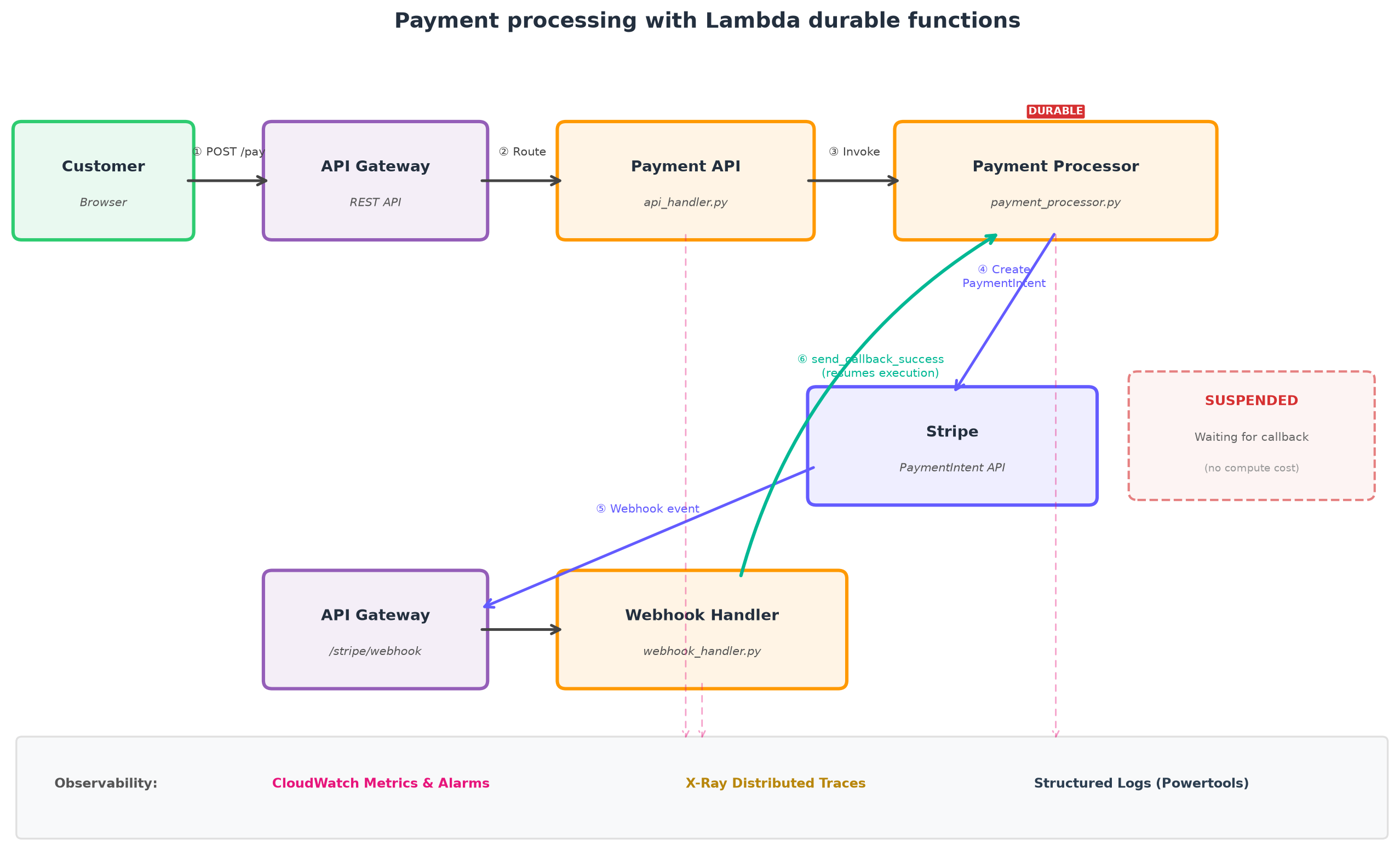
Figure 1: Payment processing flow with durable callback suspension, where the webhook handler sends the callback result back to the same suspended durable execution
The key observability challenge sits in the gap between the PaymentIntent creation (step 2) and the webhook delivery (step 3). During this period the durable function is suspended: it is consuming no compute, but it is waiting for Stripe to call back. If the webhook never arrives, the callback times out silently unless you have metrics and alarms watching for it. With proper instrumentation, you gain full visibility into this suspension gap and can diagnose issues within minutes.
You deploy the application with AWS Serverless Application Model (AWS SAM). The following template excerpt shows how we enable observability across the stack:
Tracing: Active under Globals enables X-Ray across all functions, and TracingEnabled: true on the API resource ensures traces propagate from the initial request through the entire flow.
Durable function CloudWatch metrics, custom business metrics, and alarms
Lambda automatically emits CloudWatch metrics specific to durable executions, covering execution lifecycle, capacity utilization, duration including wait time, and cost drivers. For the full list, see Monitoring durable functions.
One metric worth calling out: DurableExecutionDuration measures total wall-clock time including the callback wait period. For a payment that takes 2 seconds to process but waits 30 seconds for a webhook, this metric reports approximately 32 seconds. This is distinct from the standard Duration metric, which only measures active compute time.
Custom business metrics for the callback funnel
The built-in metrics tell you whether executions succeeded or failed. To understand where in the business flow the issue occurred, we emit custom metrics at each stage using Powertools for AWS Lambda Metrics with Embedded Metric Format (EMF):
In the webhook handler:
These metrics create an end-to-end funnel:
PaymentRequested → PaymentIntentCreated → WebhookReceived → WebhookSucceeded → PaymentSucceeded
Any drop-off between stages pinpoints the problem. If PaymentIntentCreated is higher than WebhookReceived, Stripe is not delivering webhooks. If WebhookReceived is higher than WebhookSucceeded, signature verification is failing. No corresponding PaymentSucceeded for a PaymentIntentCreated means the callback timed out.
Alarms for callback failure modes
Durable functions with callbacks have specific failure modes: callbacks that never arrive, webhook signatures that fail verification, and executions that time out waiting. We define alarms for each:
These alarm definitions are abbreviated for readability. Each alarm in the deployed template.yaml also sets Dimensions (scoping DurableExecutionFailed to the payment-processor function, and the custom metrics to their service). It also includes Statistic, Period, EvaluationPeriods, and AlarmActions/OKActions wired to an SNS topic. See the GitHub repository for the deployable definitions.
| Alarm | What it catches |
| DurableExecutionFailed | Code errors, Stripe API failures, unhandled exceptions in the durable function |
| DurableExecutionTimedOut | Whole-execution timeout: execution exceeds DurableConfig.ExecutionTimeout |
| PaymentTimeout | Callbacks that never arrive: webhook misconfiguration, Stripe outage, network issues |
| WebhookSignatureFailure | Wrong webhook secret, replay attacks, endpoint misconfiguration |
| WebhookError | Webhook function error spikes (unhandled exceptions in the handler) |
Unified dashboard
We combine built-in durable metrics, custom EMF metrics, and standard Lambda metrics into a single CloudWatch dashboard. The dashboard includes widgets for execution state, payment outcomes, end-to-end flow metrics, quota utilization, cost drivers, error breakdown, and API/webhook latency.
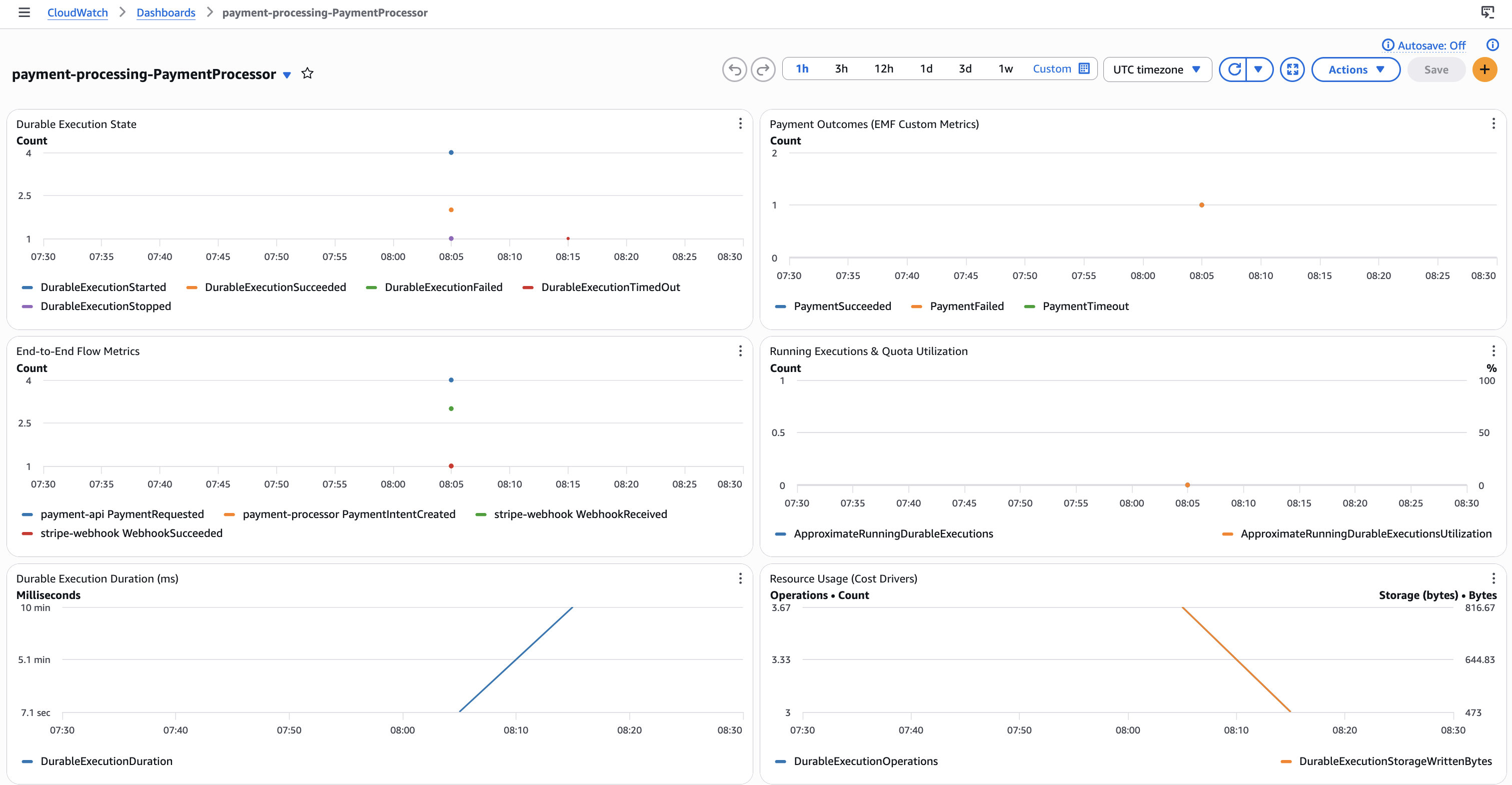
Figure 2: CloudWatch dashboard showing durable execution state, payment outcomes, end-to-end flow metrics, running executions and quota utilization
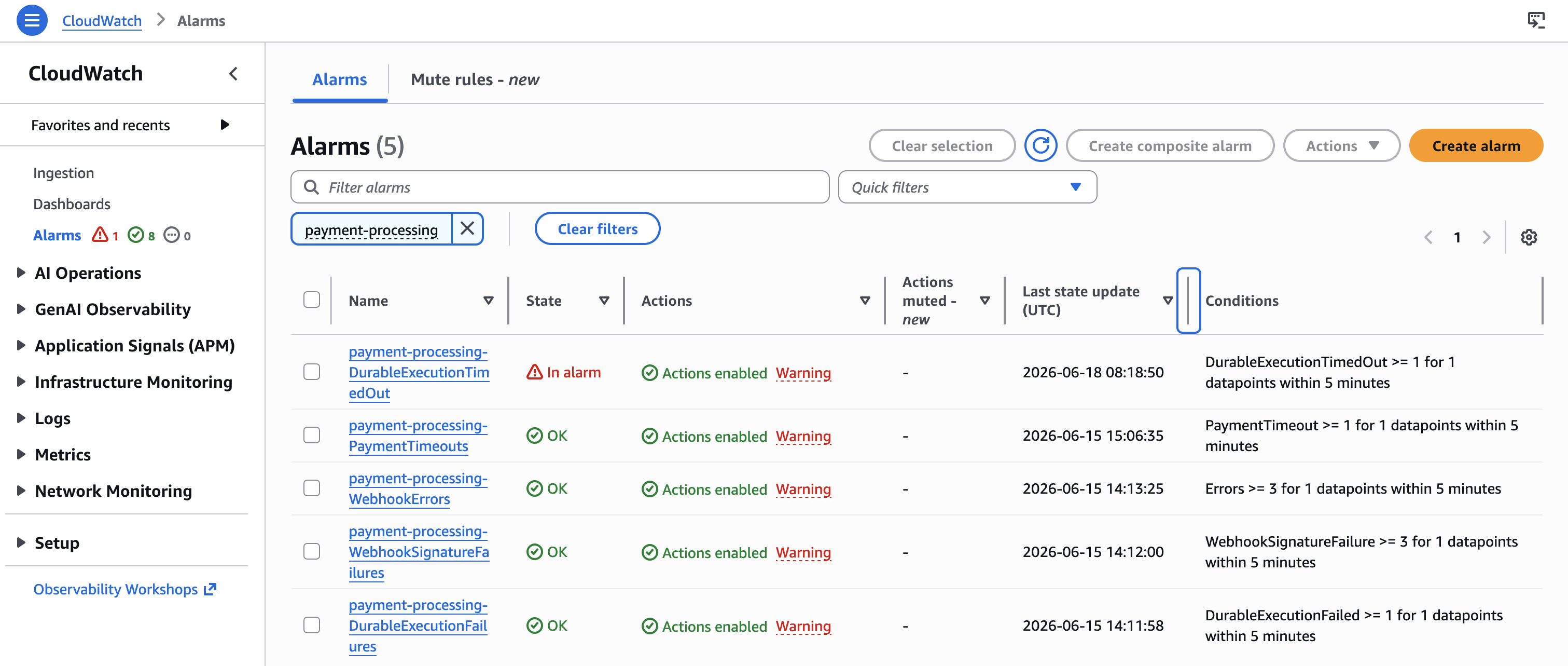
Figure 3: CloudWatch Alarms showing DurableExecutionFailures, PaymentTimeouts, and WebhookSignatureFailures alarm states
Tracing callbacks across the suspension boundary
When a durable function suspends at a callback, the execution pauses. An external system (Stripe) fires a webhook to your API Gateway, which invokes the webhook handler. The webhook handler then calls send_durable_execution_callback_success to deliver the result back to the suspended execution, which resumes and completes. The challenge is correlating these two separate invocations so you can reconstruct the full payment timeline from a single query.
Structured logging with correlation keys
Using Lambda Powertools Logger, we progressively append correlation keys as they become available. Each subsequent log entry automatically includes all previously appended keys:
In the webhook handler, we append the same keys so a single Logs Insights query reconstructs the full timeline:
Query across all three log groups for a single payment:
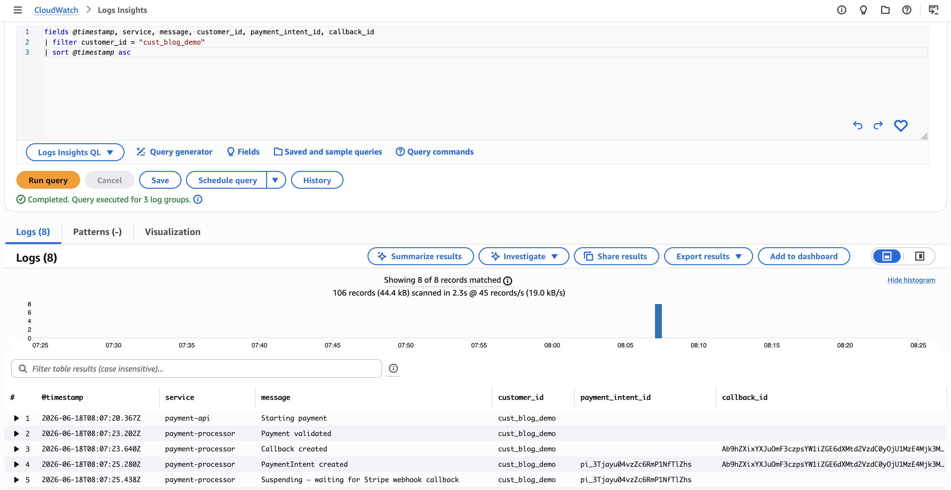
Figure 4: CloudWatch Logs Insights query showing the timeline of a single payment across payment-api, payment-processor, and stripe-webhook
Durable steps and X-Ray annotations
The SDK’s @durable_step decorator checkpoints each step. If the function crashes and replays, completed steps return their cached result without re-executing. We combine this with Powertools Tracer to add searchable X-Ray annotations at each business-critical point:
Note: The preceding code is abbreviated for readability. Refer to the GitHub repository for the complete code. The main durable handler runs within a FacadeSegment X-Ray context that does not support put_annotation(). Annotations work normally inside @durable_step functions. In the main handler, use a try/except wrapper if you need annotations outside of steps.
Note: When calling PaymentIntent.create with confirm=True, some cards decline synchronously (no webhook fires). The deployed code handles this by detecting the decline in the step return value and skipping the callback suspension, preventing an indefinite wait.
The X-Ray Service Map shows the complete request flow: API Gateway to payment-api to payment-processor, and the separate webhook path from API Gateway to stripe-webhook.
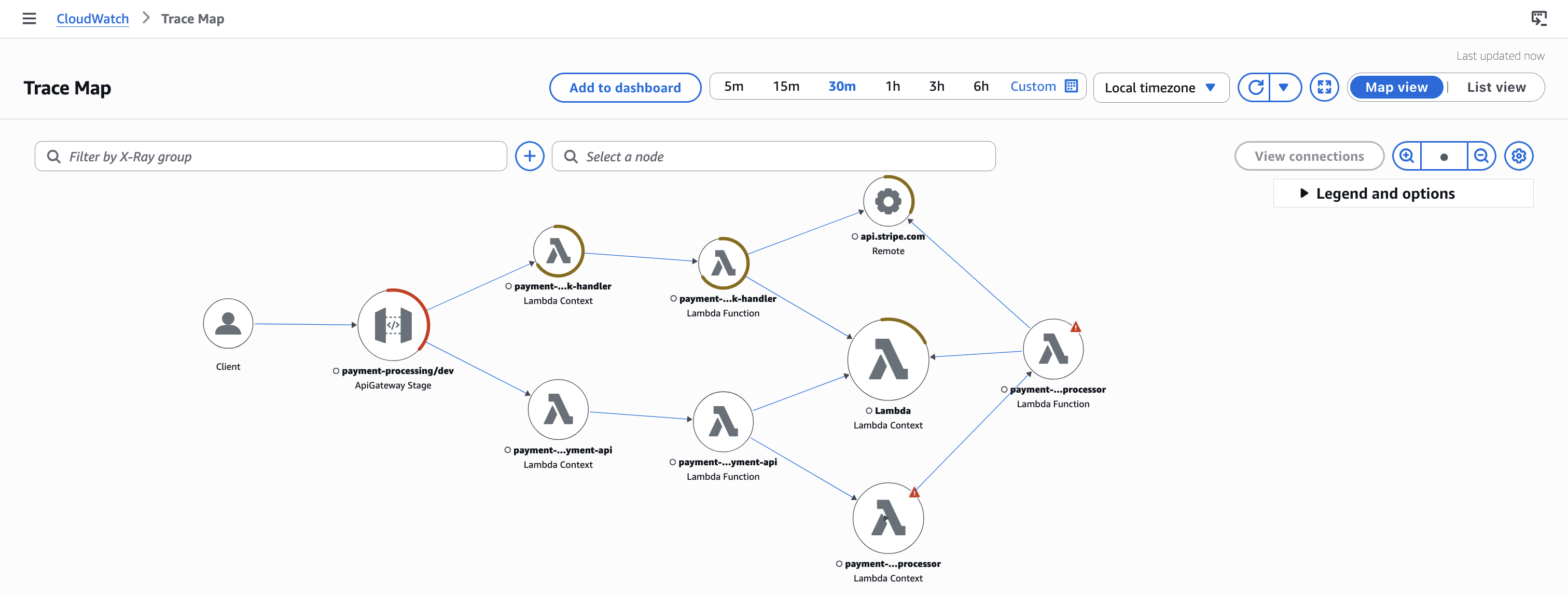
Figure 5: X-Ray Service Map showing API Gateway connected to payment-api and stripe-webhook, with payment-api connected to payment-processor
Durable executions tab
The Lambda console provides a built-in Durable executions tab showing each execution’s step-by-step timeline, including the callback wait state. You can see which steps completed, where the function suspended, and when (or if) the callback arrived.
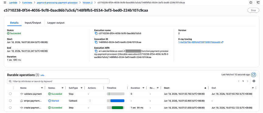
Figure 6: Lambda console Durable executions tab showing a completed execution with steps: validate-payment succeeded, create-payment-intent succeeded, stripe-payment-result callback received, and final result succeeded
Putting it together: debugging real failure modes
The following three scenarios demonstrate how all of these observability layers work together. You can reproduce each one from the demo checkout page.
Scenario 1: Webhook never arrives
A customer reports that their payment was charged but they never received a confirmation.
1. Alarm fires. The PaymentTimeoutAlarm triggers, indicating a durable execution timed out waiting for a callback.
2. Check the dashboard. The Payment Outcomes widget shows a spike in PaymentTimeout. The End-to-End Flow Metrics widget reveals the drop-off: PaymentIntentCreated count is higher than WebhookReceived, meaning the webhook never arrived.
3. Query logs. Search Amazon CloudWatch Logs Insights for the timed-out payment:
This returns the payment_intent_id of the timed-out payment.
4. Cross-reference the webhook handler. Search for that payment_intent_id in the webhook handler logs. No results means Stripe never delivered the webhook. Results with WebhookSignatureFailure mean the webhook secret is misconfigured.
5. Inspect the X-Ray trace. Filter traces by the payment_intent_id annotation. The trace shows the durable function start but no corresponding webhook handler span, confirming the webhook never arrived.
6. Check the durable executions tab. The execution shows validate-payment and create-payment-intent as succeeded, with the stripe-payment-result callback in a timed-out state.
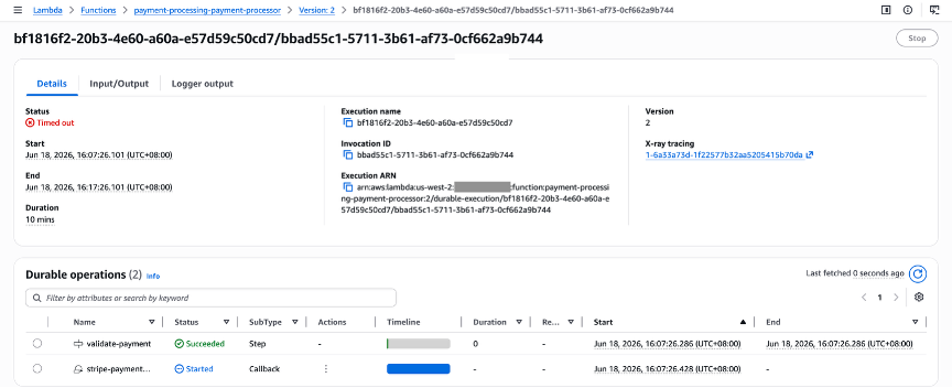
Figure 7: Durable executions tab showing the timed-out execution: validate-payment succeeded, create-payment-intent succeeded, stripe-payment-result callback timed out
Within minutes, you have identified the root cause (the Stripe webhook endpoint was misconfigured) without adding a single debug statement or redeploying code.
Scenario 2: The whole workflow runs too long
The callback timeout in Scenario 1 is a per-callback bound (5 minutes in this example). There is also an outer bound: DurableConfig.ExecutionTimeout (600 seconds), which caps the total wall-clock time of the whole execution. If you set a callback to wait an hour but the overall ExecutionTimeout is 10 minutes, the execution itself terminates first. This shows up as a distinct terminal state in the durable executions tab, on the Durable Execution State widget, and as its own alarm (DurableExecutionTimedOutAlarm).
Choose the “Simulate timeout (no webhook)” option on the demo checkout page to reproduce this. The durable function skips the Stripe call, suspends on a long-timeout callback, and lets ExecutionTimeout catch it. The dashboard distinguishes the two failure modes cleanly: per-callback timeouts show up on the custom Payment Outcomes widget as PaymentTimeout. Whole-execution timeouts appear on the built-in Durable Execution State widget alongside started/succeeded/failed counts. This distinction matters operationally because the remediation is different: callback timeouts point to external system issues (Stripe), while execution timeouts point to configuration issues (your timeout values).
Scenario 3: Customer abandons checkout
Real checkout flows have a third outcome: the customer cancels while the durable function is still suspended. The demo wires this up to StopDurableExecution, which terminates the in-flight execution and surfaces on the same Durable Execution State widget as a separate terminal state.
Choose “Simulate timeout” and then “Cancel Payment” on the demo page to see this happen. Looking at the dashboard after running all three scenarios, the execution-state widget tells the full story: started, succeeded, failed, timed-out, and stopped. Each state answers a different operational question about what is happening to your workflows.
Conclusion
In this post, we walked through observability best practices for Lambda durable functions using a Stripe payment processing pipeline. Callbacks can time out, whole executions can expire, and running workflows can be canceled. Each shows up as a distinct terminal state, and each deserves its own alarm. Layering custom business metrics, structured logging with correlation keys, X-Ray annotations, and the durable executions tab on top of the built-in CloudWatch metrics gives you a clear picture of where in the lifecycle any given execution is. It also reveals where in the business funnel any failure occurred.
Deploy the payment processing application from the GitHub repository and try the three demo scenarios to see the dashboards, alarms, and execution history in your own account. For core concepts, see Lambda durable functions. For the durable execution SDK, see the Python SDK, JavaScript SDK, and Java SDK. Browse Serverless Land for reference architectures.
WWII: The Last Day
Post Syndicated from The History Guy: History Deserves to Be Remembered original https://www.youtube.com/watch?v=tsoDi5uD0u4
Collecting CPU and memory metrics for AWS Lambda MicroVMs
Post Syndicated from Eric Heinz original https://aws.amazon.com/blogs/compute/collecting-cpu-and-memory-metrics-for-aws-lambda-microvms/
Most production services in AWS use at least two key metrics for service health – CPU and memory utilization. The amount of CPU and memory used by the host (in this case, a MicroVM) can indicate scaling signals or inefficiencies in your application. If you’re running a production workload on AWS Lambda MicroVMs, it’s recommended to have observability in these dimensions. And the easiest way to collect these metrics is through the Amazon CloudWatch Agent.
This blog shows you how to collect CPU and memory metrics from within the MicroVM using the CloudWatch Agent.
How to collect CPU and memory metrics in your MicroVM
To observe how a workload uses CPU and memory over time, run the CloudWatch Agent inside the MicroVM. Since a MicroVM image is a full OS snapshot, you can start the agent during image creation, meaning it will already be running the moment a MicroVM launches from that image. This means zero startup latency and one-time configuration: set up the CloudWatch Agent once in the image, and every MicroVM that launches from it already has a running monitoring stack.
To setup CloudWatch Agent, you will modify the ZIP containing your application and Dockerfile, and build a MicroVM image. Once you run a MicroVM from the image, three metrics will be emitted (cpu_usage_active, cpu_usage_idle, mem_used_percent) under an ImageName dimension populated from a Lambda-injected environment variable.
Lambda-injected environment variables
The Lambda MicroVMs runtime automatically exposes these environment variables to your application:
| Env var | Example |
AWS_LAMBDA_MICROVM_IMAGE_NAME |
mem-python |
AWS_LAMBDA_MICROVM_IMAGE_ARN |
arn:aws:lambda:us-west-2:…:microvm-image:mem-python |
AWS_LAMBDA_MICROVM_IMAGE_VERSION |
1.0 |
AWS_REGION |
us-west-2 |
The example below uses AWS_LAMBDA_MICROVM_IMAGE_NAME as a metric dimension so you can monitor metrics per MicroVM image.
Setting up custom metric dimensions from env variables
Amazon CloudWatch Agent uses telegraf to process metrics and opentelemetry-collector (OTel) to export them. Normally, you configure the agent through a cwagent.json file, which the agent’s config-translator converts into a telegraf TOML file and an OTel YAML file for the process to use at startup.
In this post, we skip the JSON configuration and create the telegraf and OTel files directly. This lets us dynamically set a custom metric dimension from an environment variable using OTel’s ${env:VAR} syntax. The telegraf config defines which metrics to collect, while the OTel config resolves the environment variable at process start and appends it as a dimension.
Configuring CloudWatch Agent
In this section, we cover how to configure CloudWatch Agent to report CPU and memory metrics for MicroVMs launched from your MicroVM image.
Step 1: Configure the telegraf plugin to emit CPU and Memory metrics
Create a cwagent.toml file to define the configuration for telegraf to emit CPU and memory metrics every minute:
In this configuration, the chosen metric (used_percent) reports memory usage as a percentage of total memory inside the MicroVM. Telegraf derives this from MemAvailable in /proc/meminfo, which reflects memory that is committed and not reclaimable. When your application releases memory back to the OS (e.g. via free()), that memory becomes reclaimable again, and used_percent decreases accordingly.
To monitor additional memory metrics, you can add the following fields to the fieldpass list:
cached: for page cache bytesbuffered: for buffered I/O bytestotal: for total memory available to the MicroVM
Step 2: Configure OTel to process and export the metrics to CloudWatch
Create a cwagent.yaml file to export metrics to CloudWatch under the namespace LambdaMicroVms/Application with dimension ImageName. The dimension value is populated from the environment variable AWS_LAMBDA_MICROVM_IMAGE_NAME.
If you want more dimensions such as image version, add it to attributes.
Note: since only aggregate CPU usage is emitted by telegraf, we don’t need OTel to include a CPU dimension, so delete_key(attributes, "cpu") is used to remove this dimension.
Step 3: Install CloudWatch Agent in your Dockerfile
In your Dockerfile, install the CloudWatch Agent from the Amazon Linux repository. Then copy over the telegraf and OTel files to where the agent expects to retrieve them. Then configure your application’s entrypoint:
Step 4: Configure your Entrypoint to start CloudWatch Agent
Create a file called entrypoint.sh to start the CloudWatch Agent as a background process while executing your application in the foreground:
This is everything you need to get CloudWatch running inside your MicroVMs!
Execution role requirements
To write the metrics to CloudWatch, ensure the MicroVM’s execution role has cloudwatch:PutMetricData permissions.
Verifying it works
To verify the metrics are being emitted, run the following command a few minutes after launching a MicroVM from your image:
You should see exactly three metric series per image: cpu_usage_active, cpu_usage_idle, and mem_used_percent.
Viewing the metrics
To view the metrics in the CloudWatch console, click “All Metrics”, and select the custom namespace LambdaMicroVms/Application (set in cwagent.yaml namespace field).
Here is an example for how it looks inside the console:
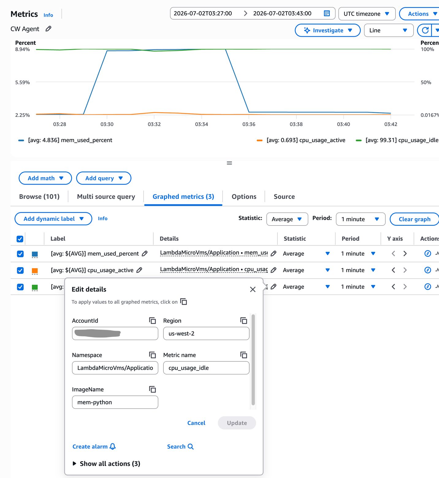
In the graph above, the application consumes ~2% memory (left axis) and < 0.1% CPU usage (right axis) when idle. The application then consumes ~9% of memory at the 30 minute mark, holds it for around 5 minutes, then releases it back to the OS. As it releases memory, we see memory utilization decrease. In this example, the MicroVM size is larger than the application needs – less than 10% of memory was used, indicating a smaller MicroVM size may be more economic for this workload.
If your CPU and/or memory utilization is below the baseline size configured (see MicroVM sizing), consider choosing a lower baseline to reduce your compute bill.
Conclusion
This post shows you how to configure and run the CloudWatch Agent inside your MicroVM image so you can collect CPU and memory metrics for MicroVMs launched from the image. This helps you monitor resource usage of your application as it is used, so you can right-size the MicroVM for your workload, debug service health, and check for scaling signals.
To get started, visit the AWS Lambda console, or install the AWS Lambda MicroVMs agent skill.
If the Markets Reject OpenAI and Anthropic, the US Should Nationalize Them
Post Syndicated from Bruce Schneier original https://www.schneier.com/blog/archives/2026/08/if-the-markets-reject-openai-and-anthropic-the-us-should-nationalize-them.html
This essay was written with Nathan E. Sanders, and originally appeared in The Guardian.
OpenAI, and then Anthropic, were each formed by AI developers who feared unrestrained corporate AI development—specifically, that companies like Google and Meta would steer the technology towards deleterious, maybe even catastrophically unsafe, outcomes for society. Their founders proclaimed that their new labs, uniquely, could be trusted to develop the technology in humanity’s best interest. But each, in turn, were themselves co-opted by the same market incentives, themselves becoming corporate behemoths zealously guarding future investor value rather than the public interest.
It was only a few weeks ago, in June, when OpenAI and Anthropic each filed for their IPOs and were met with buzz about trillion-dollar valuations. The hype around their valuations is so extreme that many worry about their potential for concentrating wealth on a global scale. In an effort to leave something for the rest of us, some observers have proposed that the federal government seize a share of these companies’ stock to create a US sovereign wealth fund, or redistribute their revenues to produce a dividend for taxpayers.
Now the headlines are about public backlash to AI datacenters and the AI chip giant Nvidia’s slumping stock. The tech and AI giant SpaceX’s newly minted stock price tanked just weeks after its IPO. There are even questions about whether the leading AI labs will ever be sustainably profitable. All of a sudden, the makers of ChatGPT and Claude face strong headwinds as they seek to generate the massive equity assets that once felt all but assured.
In fact, evidence suggests the market itself could reassess that these companies offer nothing of financial value. In that case, perhaps we can return them both to their original purposes. If these AI companies should fail in the financial markets, the US should nationalize them and convert them into national labs operated under democratic control that preserve their benefit to the public interest.
The economics of the big AI labs hardly guarantee a booming return on investment. Frontier AI models are both expensive to train and depreciate within months, when a newer model appears. This means that the payback window to extract profit from them is very narrow. Meanwhile, enterprise clients are getting smart about minimizing AI token usage. Even worse, the models are basically commodities; the best ones largely perform and behave similarly, which depresses prices. Perhaps most importantly, open-source and Chinese competitors—lagging only a few months behind the leading labs in capability—give away for free the kinds of models Anthropic and OpenAI sell.
Even setting aside the model training costs, it’s not clear whether the unit economics of AI as it’s currently conceived will ever be sustainably profitable. Many of these free and open-source models can be run locally: the large ones on private clouds and high-end servers, the smaller ones on anyone’s laptop or even cellphone, putting to question the companies’ exorbitant capital investment in datacenters.
It’s not that OpenAI and Anthropic are not valuable as organizations. They have remarkably talented AI scientists and engineers that are continuously producing innovations driving a global mania for their offerings. These leading labs might not ever be profitable, but their products are doing a lot of good in the world. You may or may not be a user of or believer in their technology, but their staggering, ongoing usage growth suggests that an awful lot of people would be disappointed if the companies simply disappeared.
The problem isn’t the people or the products, it’s the system. As constituted, OpenAI and Anthropic may not be valuable as market equities. If the market assesses they are not capable of producing a growing financial return on investment for shareholders, the companies will collapse.
Maybe private, for-profit is just not the right economic model under which to develop AI. Perhaps OpenAI should be returned to its private non-profit roots, the legacy they fought so hard to change and which Anthropic’s founders spurned. Or possibly both could be reorganized as research centers at universities, returning to academia the scores of high-profile research faculty they have poached.
But a better outcome for society would be to establish public ownership and operation of their product-oriented capabilities. Turn OpenAI and Anthropic into US government agencies producing AI as a public good.
Transitioning the big AI labs into public agencies would require some restructuring. We can separate these companies into two pieces: product innovation and compute operations. The innovation function can be publicly managed, akin to national labs. Congress could provide more rigorous oversight than the kind of unfettered venture capital these labs have recently had access to. The US has a long, successful history of these kinds of institutions, which have produced world-shaping innovations in spaceflight, telecommunications, nuclear power and more. Congress currently manages a $200bn R&D portfolio, within which frontier AI development is, arguably, a glaring gap.
AI operations could be managed as a commodity resource, like public electrical or water utilities: local or regional ownership, nationwide distribution and strict regulation on how they balance fee extraction from ratepayers with raising capital for infrastructure investment. Although AI datacenters are not the same as power or water treatment plants, the US also has a long history of managing national, regional and state supercomputing centers.
Other countries, including Switzerland, Spain and Singapore, are already operating public AI labs. They also have national supercomputing centers already providing public access for running AI models for general use, as do Germany and Australia.
The benefits to the public are clear. Through democratic oversight, the most important AI models could become open, transparent and responsive to the demands of the public rather than private shareholders. They could be aligned to democratic values rather than corporate profits, never taking advertiser money to promote certain brands and training on only appropriately licensed data. And they could be set to focus on the realistic and pro-social goal of maximizing the usefulness of AI to society rather than the fanciful and anti-social goal of supplanting humans with artificial general intelligence.
By emphasizing scientific cooperation rather than corporate competition, we could also reduce the overall resource and environmental cost associated with AI. Instead of perpetually dueling training runs of each companies’ models at ever large scales targeted to fuel investor hype, we could limit AI training resources based on cost and benefit to the public.
What’s in it for the companies themselves and their employees, who sacrifice hypothetical billions in equity by ceding to public ownership? A return to their roots and to their core mission of developing AI safely in the public interest, if they are serious about it. Both companies are theoretically bound through their governance structures to prioritize mission over profit anyway (not that anyone really thinks that’s how they currently operate).
To be clear, we’re not advocating for a golden parachute for the executives or investors, or for continuing the outlandish pay rates of the most highly remunerated AI researchers. If the public is footing the bill, these compensation packages should be aligned to the civil service and those employees not satisfied with that can go elsewhere—if the business models of any remaining private labs still support much higher pay.
While we believe that these companies are unsustainable as private firms, the timeline remains unclear. Their primary investor story is that AI is a race to “artificial general intelligence”—the kind of AI you’re used to from science fiction. The bet seems to be that the two companies can convince enough people that this outcome will turn them a profit, go public, and then make their investors and employees rich before the bubble bursts.
But suppose that the bubble bursts. If the US is smart, it will catch the companies as they fall. Regardless of what the markets think, to the public, they’re too valuable to let die.
Serverless vehicle tracking at scale: Bosch L.OS on AWS
Post Syndicated from Yogish Kutkunje Pai original https://aws.amazon.com/blogs/architecture/serverless-vehicle-tracking-at-scale-bosch-l-os-on-aws/
When Bosch Mobility Platform Solutions set out to unify vehicle tracking across India’s fragmented spot logistics market, they faced a daunting reality: dozens of telematics providers, incompatible data formats, and thousands of concurrent tracking requests — all needing real-time resolution. The result was L.OS, a serverless platform on AWS that standardizes this chaos into a single visibility layer.
In this post, we’ll show you how Bosch Mobility Platform Solutions (MPS) uses AWS services to solve these challenges through their L.OS solution. You’ll learn how Bosch built a scalable, serverless architecture that standardizes and integrates multiple tracking data sources, so you can achieve real-time visibility and data-driven decision-making across complex logistics networks.
Key challenges in logistics visibility
If you manage a modern supply chain, you face several critical challenges:
- Data fragmentation and integration complexity.
- Multiple tracking systems with incompatible data formats.
- Different communication protocols across providers.
- Lack of standardization in data exchange.
- Complex and costly point-to-point integrations.
- Operational inefficiencies.
- Manual coordination between stakeholders.
- Time-consuming reconciliation of conflicting information.
- Difficulty in providing accurate ETAs.
- Limited real-time visibility into shipment status.
- Scale and performance issues.
- High volume of concurrent tracking requests.
- Variable data quality from different sources.
- Performance bottlenecks during peak operations.
- Cost implications of real-time tracking.
- Regional complexities.
- Fragmented spot logistics networks.
- Multiple intermediaries in the supply chain.
- Varying levels of technological adoption.
- Regional compliance requirements (such as AIS140 and FASTag in India).
Introducing L.OS on AWS: A unified visibility solution
To address these challenges, Bosch’s Logistics Operating System (L.OS) on AWS provides a horizontal integration layer that connects previously siloed logistics solutions. The solution features a service catalog where solution providers and consumers can collaborate to solve complex use cases, fostering innovation in the logistics sector. Let’s explore how L.OS enhances vehicle visibility through its core workflows: discovery, tracking, and termination.
Discovery
When a client needs to track a vehicle, the service app makes a discovery call to the L.OS gateway. This call includes essential details such as the vehicle number plate or vehicle identification number (VIN). Upon receiving the request, the L.OS solution performs necessary authentication and authorization. L.OS then broadcasts the request and waits for acknowledgment from one or more connected participants. The responses contain information such as the mode, frequency, and reliability of tracking, which can be used for shortlisting and decision-making.
The following diagram illustrates the discovery workflow, showing how a client’s tracking request flows through L.OS to connected participants and back.
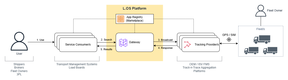
Figure 1 – The discovery flow: the service app sends a discovery call to the L.OS gateway with vehicle identifiers. L.OS broadcasts the request to connected participants, collects acknowledgments containing tracking mode, frequency, and reliability details, and returns them to the consumer for shortlisting.
Tracking
Once the consumer has selected a vehicle and a service provider (if there are multiple options), a request is sent to the L.OS to initiate tracking. This request is relayed to the specific service provider. The tracking mode determines who must grant consent. For SIM tracking, a consent request goes to the driver. For GPS tracking, it goes to the fleet owner. The solution waits for the tracking provider to create the trip. Upon receiving confirmation, L.OS registers the tracking request and provides a unique tracking ID to indicate that tracking has been initiated. From here, the consumer is asynchronously notified of the vehicle’s location at the specified frequency, or the maximum frequency supported by the service provider, whichever is faster. Consumers can also request the live location of the vehicle at any time between the regular reporting intervals.
The following diagram shows the tracking workflow, from initiation through consent, trip creation, and ongoing location updates.
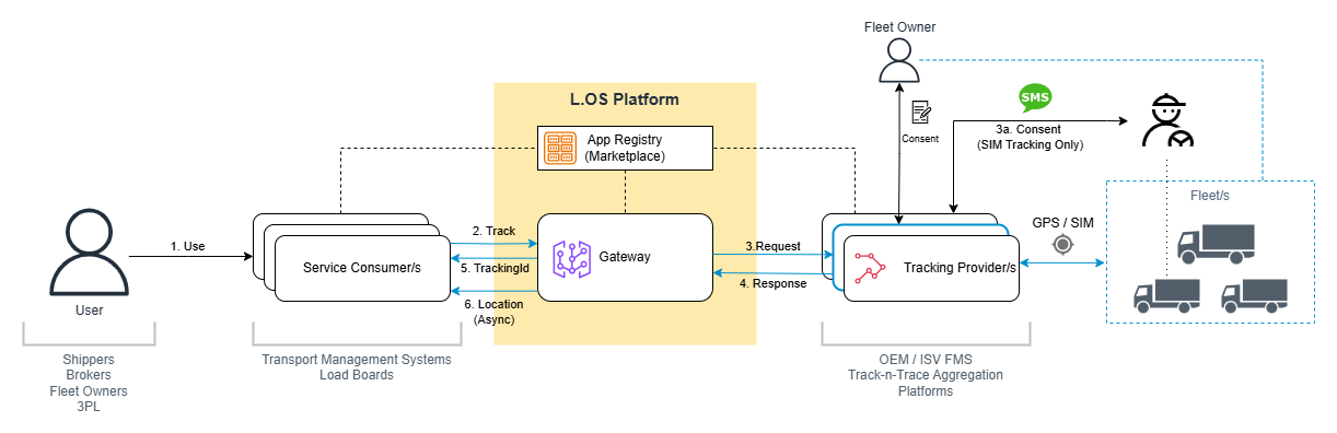
Figure 2 – The tracking flow: the consumer sends a tracking request to L.OS, which relays it to the selected service provider. A consent request is issued (to the driver for SIM tracking, or the fleet owner for GPS tracking). Once the provider confirms trip creation, L.OS returns a unique tracking ID and begins delivering asynchronous location updates at the agreed frequency.
Termination
The tracking is automatically terminated when the vehicle enters the destination geo-fence. Alternatively, tracking can be terminated manually by sending an explicit request to L.OS, which is then relayed to the service provider.
Architecture overview
The L.OS solution built on AWS uses various services to create a scalable, secure, and maintainable system. The architecture implements serverless components (AWS Lambda adapters) where appropriate while using containers (Amazon Elastic Container Service (Amazon ECS) with AWS Fargate) for the core connector service. Let’s explore how these AWS managed services work together to create a flexible and scalable integration solution. The following diagram shows the end-to-end architecture, illustrating how requests flow from client applications through the API layer, into the core connector service, and out to individual tracking providers.
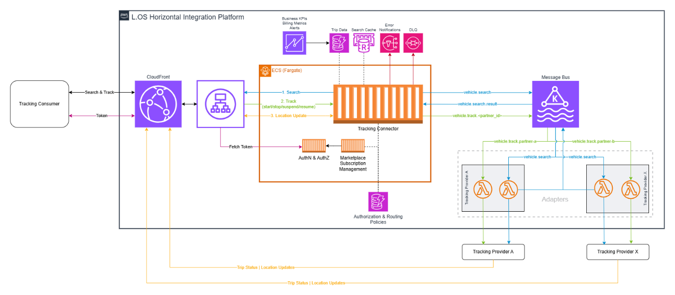
Figure 3 – L.OS architecture on AWS: Client applications connect through Amazon API Gateway to the Tracking Connector running on Amazon ECS Fargate, which handles protocol standardization, routing, and session management. Provider-specific Lambda adapters translate between the standardized connector API and each tracking provider’s API. Amazon MSK serves as the event bus for asynchronous location updates. Amazon ElastiCache provides low-latency caching for frequently accessed data, Amazon DynamoDB stores business rules and security policies, and the Marketplace Subscription Management service (also on Fargate) handles authentication, customer relationships, and provider configurations. Amazon QuickSight delivers real-time monitoring and usage analytics.
Key components
The architecture comprises five core components that work together to deliver reliable, real-time vehicle tracking at scale. Each component handles a distinct responsibility — from protocol translation to event streaming — allowing the system to scale and evolve independently.
Centralized orchestration with Amazon ECS Fargate
The Tracking Connector, running on Amazon ECS Fargate, serves as the central orchestration layer. It handles critical functions including:
- Protocol standardization across multiple providers.
- Intelligent request routing.
- Response aggregation.
- Session management.
- Comprehensive error handling.
- Performance optimization using Amazon ElastiCache.
Serverless provider integration
We use AWS Lambda to implement Tracking Adapters that handle provider-specific transformations. These adapters efficiently translate between our standardized connector API and various provider APIs, allowing for easy onboarding of new providers.
Event-driven communication
Amazon MSK (Managed Streaming for Apache Kafka) powers our message bus, enabling:
- Standardized topic patterns.
- Support for multiple domain connectors.
- Real-time data streaming for tracking, parking, vehicle health, charging, and fleet management.
Subscription and access management
The Marketplace Subscription Management service, deployed on Amazon ECS Fargate, manages:
- Customer relationships.
- Service consumer configurations.
- Provider integrations.
- Authentication and authorization token claims.
Policy and security enforcement
We use Amazon DynamoDB to store and manage:
- Business rules.
- Security policies.
- Authorization configurations.
- Routing rules.
Monitoring and analytics
Amazon QuickSight provides:
- Real-time system performance metrics.
- Usage analytics.
- Health monitoring.
- Anomaly detection.
Benefits
By implementing this serverless architecture on AWS, Bosch L.OS achieved significant improvements in vehicle tracking capabilities:
Operational efficiency
The combination of standardized Lambda adapters and the centralized Tracking Connector on ECS Fargate eliminates the manual coordination that previously slowed provider onboarding. Where ISVs once spent 2–4 weeks on bespoke integration work for each new customer request, the standardized connector API and adapter pattern reduces this to within 3 days. Real-time data validation at the connector layer — before events reach downstream consumers — also improves data accuracy by catching format inconsistencies at ingestion rather than during reconciliation.
Scalability and performance
Because the core connector runs on Fargate with auto-scaling task definitions, and each provider adapter is an independent Lambda function, the system scales horizontally without manual intervention. Bosch’s deployment currently handles 35,000 trips per day — each generating multiple location events — with sub-second response times for 99.9% of tracking queries. As new ISVs are onboarded, additional Lambda adapters are deployed independently, so scaling the provider network does not add load to existing integrations.
Cost optimization
Integrations in fragmented logistics markets often stall because multiple vendors must coordinate through manual processes — handoffs, SIM card provisioning, consent management, and troubleshooting. By automating these workflows within the L.OS connector layer and MSK event bus, Bosch estimates integration costs are reduced by 15–20%. The architecture also removes per-vendor overhead (SIM management, consent flows, provider-specific troubleshooting) that was previously passed on to small transporters. This potentially lowers their total tracking costs by 25–30%.
Enhanced customer experience
The unified API Gateway endpoint and MSK-powered event streaming mean consumers receive location updates from any connected provider through a single interface — regardless of the underlying tracking technology. What previously required hours of manual coordination across providers now surfaces as a consolidated event within approximately 1 minute, according to Bosch. Improved ETA accuracy is a direct result: with standardized, high-frequency location data flowing through ElastiCache, downstream planning systems can compute more reliable arrival predictions.
Compliance and security
DynamoDB-backed policy enforcement ensures that business rules, authorization configurations, and regional compliance requirements (such as India’s AIS140 and FASTag mandates) are evaluated consistently on every request. The built-in security features of AWS — IAM roles, virtual private cloud (VPC) isolation, and encryption at rest and in transit — provide the baseline. Automated audit trails captured through the event bus give organizations a verifiable record of all tracking operations.
L.OS growth
L.OS is currently operational in India with 10 integrated ISVs. The serverless adapter pattern makes geographic expansion straightforward: new region-specific adapters can be deployed as independent Lambda functions without modifying the core connector. Bosch plans to use this approach to expand into Europe for trailer monitoring use cases.
Conclusion
In this post, we showed how Bosch built L.OS, a serverless vehicle tracking platform on AWS that unifies fragmented logistics visibility into a single integration layer. By using AWS services such as Amazon ECS with Fargate for centralized orchestration and AWS Lambda for provider-specific adapters, the architecture standardizes multiple tracking providers into a unified API.
This standardization eliminates the need for maintaining multiple point-to-point integrations, freeing you to focus on core operations instead of managing repetitive integration tasks. Through strategic collaboration with key stakeholders in the visibility solutions space, L.OS is helping businesses achieve measurable outcomes: enhanced customer experience, increased operational agility, reduced operational expenses, and improved profit margins.
What started as a vehicle tracking solution is now evolving into a broader mobility services portfolio, powered by the scalable infrastructure that AWS provides. This evolution positions L.OS to address not only today’s tracking needs, but a broader range of logistics use cases as they emerge.
If you have questions or feedback about this post, leave a comment in the comments section.
- To learn more about the AWS services used in this solution, explore these resources:
- Explore the sample code for this solution on GitHub — includes Infrastructure as Code templates, Lambda function source code, and step-by-step deployment instructions.
- Building real-time fleet tracking applications on AWS
- Best practices for container-based applications using Amazon ECS
- Implementing event streaming with Amazon MSK
For more information about the Bosch L.OS solution and its capabilities, visit Bosch L.OS website.
Contact your AWS account team to learn how we can help you build similar solutions for your logistics operations.
About the authors
Comic for 2026.08.14 – The Good Book
Post Syndicated from Explosm.net original https://explosm.net/comics/the-good-book
New Cyanide and Happiness Comic
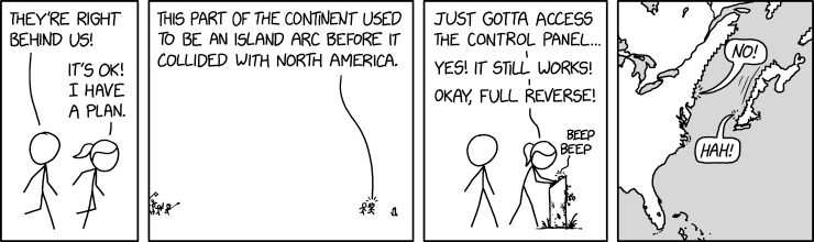
Accretionary Arc
Post Syndicated from xkcd.com original https://xkcd.com/3285/
Great Odin’s Raven! What is this thing?!
Post Syndicated from Matt Granger original https://www.youtube.com/shorts/0QNL6Mv5UrU
AWS Certificate Manager will discontinue email validation to prove domain validation for certificates
Post Syndicated from Adam Aboudi original https://aws.amazon.com/blogs/security/aws-certificate-manager-will-discontinue-email-validation-to-prove-domain-validation-for-certificates/
Today, we’re announcing that AWS Certificate Manager (ACM) will discontinue support for email-validated public certificates by September 30, 2027. If you use email validation for your ACM public certificates, you need to migrate to DNS validation before that date. This change aligns with the Certification Authority/Browser (CA/B) Forum’s industry-wide deprecation of email-based domain validation and gives you a full year to migrate ahead of the Forum’s March 2028 deadline.
In this blog post, we share the rationale for this change, the timeline, and the steps you can take to migrate your certificates to DNS validation.
Background
The CA/B Forum sets the standards that browsers and certificate authorities must follow for publicly trusted certificates. In November 2025, they voted to end support for email-based domain validation effective March 15, 2028. After that date, certificates validated through email won’t be trusted by browsers, regardless of which certificate authority issued them.
ACM will be deprecating its email validation in-line with the CA/B Forum’s requirements, by September 30, 2027. The ACM timeline gives customers one year to migrate before the CA/B Forum’s hard deadline.
Timelines for these changes
If you currently use email validation for certificates requested from ACM, there are a few important dates that you should be aware of:
- January 1, 2027: ACM will no longer offer email validation in new AWS Regions.
- March 31, 2027: ACM will no longer offer email validation for new certificate requests in any Region.
- September 30, 2027: ACM will no longer renew existing certificates that use email validation in any Region.
- March 15, 2028: Per the CA/B Forum, public certificate authorities can no longer use email-based domain validation to issue or renew publicly trusted certificates. Certificates issued before this date remain valid until they expire.
Check for existing email validated certificates
If you have any ACM issued public certificates, you can check whether any of them are email validated by using the AWS Management Console for ACM or the AWS Command Line Interface (AWS CLI).
Identify email validated certificates using the ACM console
Use the following steps in the console to find email validated certificates.
- Open the ACM console.
- Select the filters Validation method = Email and Type = Amazon Issued for a list of email validated certificates.
- Any certificates listed are public email-validated certificates and should be migrated before September 30, 2027.

Figure 1: List of all public email validated certificates
Identify email-validated certificates using the AWS CLI
Use the following commands to find email validated certificates.
Migrate existing email validated certificates
To assist you in this migration, ACM is updating the UpdateCertificateOptions API so you can switch a certificate’s validation method from email to DNS in place. This means the certificate Amazon Resource Name(ARN) will remain the same and no changes will be needed to your AWS resources that reference the certificate.
When you update a certificate to DNS validation, ACM provides a CNAME record to add to your DNS configuration, and you have 72 hours to add that record. During this window, the certificate continues to function normally on email validation. If the 72 hours elapse without a DNS update, the certificate stays active on email validation and you can retry when ready. After DNS validation is complete, ACM is designed to automatically renew your certificate before it expires without further manual intervention required. We recommend completing migration before September 30, 2027, so that ACM can keep your certificates up to date without interruption.
To migrate using the console
- After you’ve identified a certificate that needs updating, open it and select Update validation method at the top of the page.

Figure 2: DNS Validation prompt when viewing an email validated public certificate.
- After the update is triggered, you will see a View DNS records flashbar at the top of the certificate page.

Figure 3: View DNS validation records after updating validation method.
- Select View DNS Records in the flashbar to open a dialog box from which you can download the CSV file for the CNAME records to export to other DNS providers.

Figure 4: Get DNS validation information from the dialog box
- For Route 53 users, there is a Create records in Route 53 that makes the validation available as a one-click option.

Figure 5: Create DNS validation records into Route 53
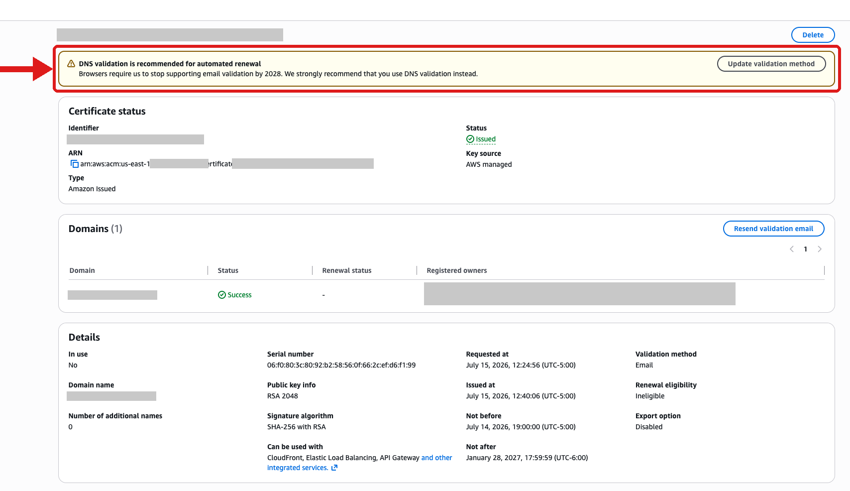
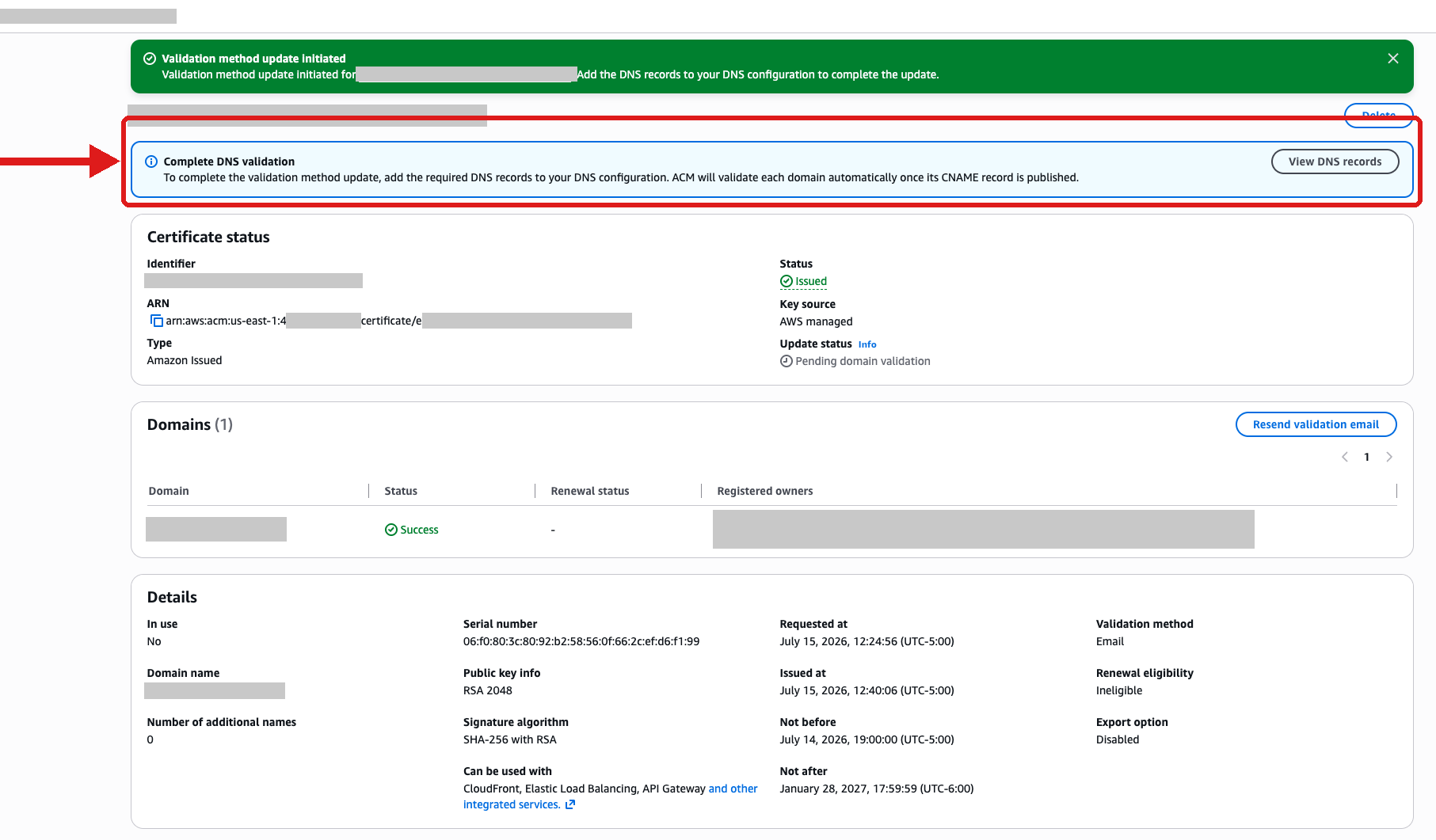
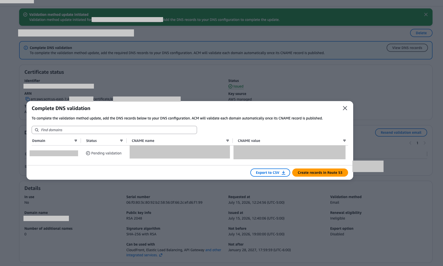
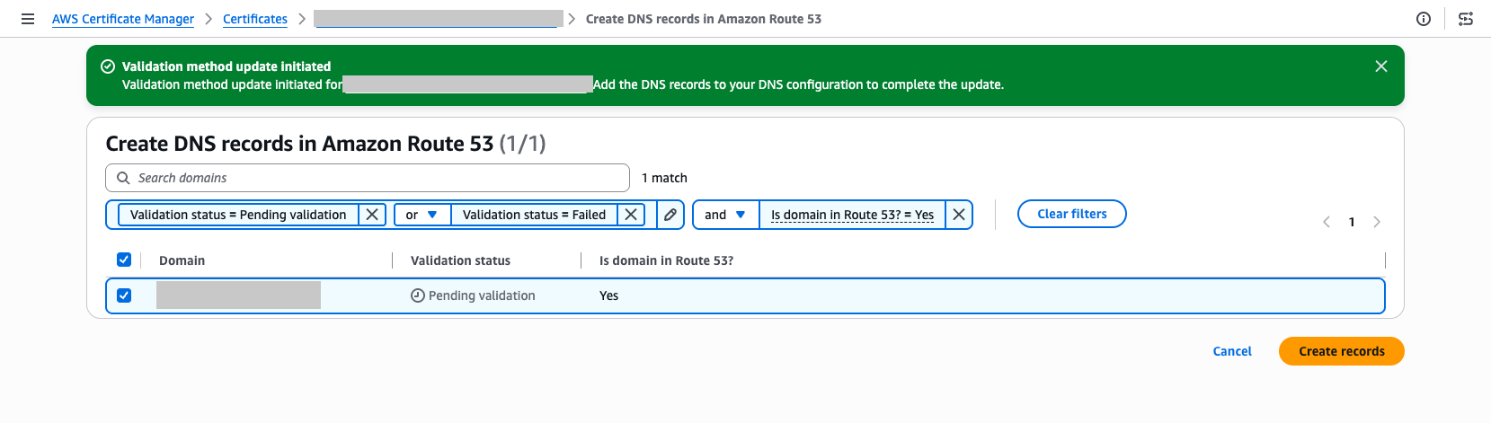
To migrate using the AWS CLI:
For instructions on how to update certificates using the AWS CLI, see the email to DNS migration user guide.
Alternatives after email validation is no longer available
ACM supports two validation methods for new certificates going forward:
- DNS validation – Add a CNAME record to your DNS configuration. ACM automatically renews DNS-validated certificates as long as the record remains in place. We recommend this method for most use cases.
- HTTP validation for CloudFront – ACM provides a unique token that you host at a well-known URL path on your domain. This method is only available for certificates used with Amazon CloudFront.
Both methods remove the manual approval step required by email validation and let ACM renew your certificates automatically.
Conclusion
The deprecation of email validation and use of the new UpdateCertificateOptions API helps keep your certificates trusted and your applications running as industry standards evolve. The updated UpdateCertificateOptions API is designed to make this migration straightforward: switch your validation method in place, add the DNS record, and ACM is designed to handle renewals automatically from that point forward.
If you have questions or need assistance migrating, contact AWS Support or start a new thread on the AWS re:Post ACM Forum.
If you have feedback about this post, submit comments in the Comments section below.
Designing for failure: Building resilient systems on AWS
Post Syndicated from Dhvani Vora original https://aws.amazon.com/blogs/compute/designing-for-failure-building-resilient-systems-on-aws/
In cloud computing, failure in distributed systems isn’t a matter of if, but when. Modern applications span servers, Availability Zones, and Regions. Each component represents a potential point of failure. Resilient applications engineer fault tolerance into their architecture, building systems that self-recover and maintain availability. This post is written for engineers and architects who run distributed data systems such as Apache Cassandra, Apache Kafka, or HDFS on Amazon Elastic Compute Cloud (Amazon EC2) and want to build resilience against hardware failure.
We were working with a customer during one such incident and wanted to share the example. The customer runs a web application that uses Cassandra as its data store, handling both read-heavy and write-heavy workloads at a scale of millions of queries per day.
The 2 AM wake-up call nobody wants
Consider a platform that monitors millions of enterprise network devices across hospitals, universities, and airports worldwide. It detects problems before IT teams even notice them. For that platform, a 2 AM page is more than inconvenient. When your value proposition is catching failures before anyone else does, being caught off-guard by your own infrastructure failure is existential.
The engineering team was deep in quarterly planning when their monitoring dashboard lit up. Three Cassandra nodes had gone dark simultaneously. This was not a graceful shutdown or a rolling restart. It was a hard failure with no warning.
Their architecture is typical of high-scale telemetry platforms. Kafka-powered microservices ingest device telemetry, Apache Flink handles real-time anomaly detection, and Apache Airflow orchestrates batch analytics and firmware updates. All of these rely on Apache Cassandra as the distributed database backbone. The database stores billions of daily writes and handles millions of queries per day.
What actually happened
Three i4i.4xlarge instances running Cassandra nodes failed simultaneously in the SFO region. Investigation revealed that all three instances were colocated on the same physical host. That host suffered a hardware failure, taking all three instances offline at once.
Engineers spent ninety minutes digging through system logs trying to determine the root cause. The root cause was architectural. The deployment lacked Partition Placement Groups, creating a single point of failure where logical replication was undermined by physical collocation.
The good news: Cassandra maintained service availability with no data loss thanks to its replication factor. The bad news: for over an hour, the system ran on a thin safety margin. One more node failure in the same replication group would have caused data unavailability for a subset of queries. That is real customer impact for a platform that promises always-on monitoring.
This is the insidious nature of correlated failures. Individual node failures are expected and designed for. That is the whole point of replication. But when your replicas share physical infrastructure, replication becomes a paper guarantee. You have three copies of the data, but they all live on the same machine.
Making matters worse, their monitoring tools completely missed the initial failure. System status checks correctly flagged the host-level problem. But without Amazon CloudWatch alarms configured to act on those checks, detection was entirely reactive. The team found out because other things started behaving oddly, not because an alarm told them three nodes were down.
Hardware fails. You can’t fix it with a patch or configuration change. The real questions are how fast you detect it, how well your system handles it, and whether failures are correlated.
How the team responded and what they changed
The operations team manually replaced two failed instances with new ones on healthy hardware and restarted the third for log collection. Once replacement instances came online, new Cassandra nodes automatically rejoined their clusters and streamed data from surviving replicas. This process took several hours depending on data volume. Only after full synchronization did the clusters return to full redundancy.
The team recognized that this ninety-minute manual scramble wouldn’t scale. Similar problems had happened before, and each time they followed the same reactive pattern: page, investigate, manually replace, wait for streaming, breathe. Here’s what they implemented to break that cycle, and what you should implement too.
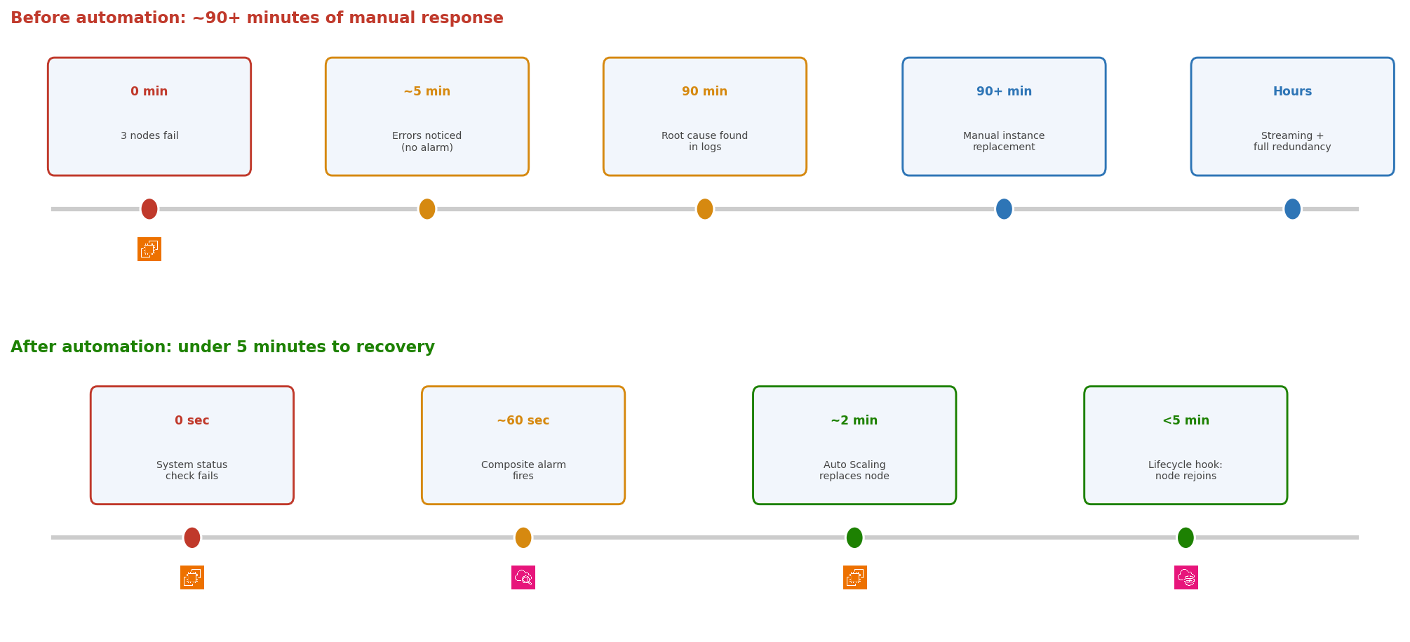
Figure 1: The same failure handled two ways. Manual response took over 90 minutes plus hours of streaming. The automated path completes recovery in under 5 minutes.
1. Use Partition Placement Groups to isolate failure domains
The three crashed servers shared a physical machine because no one told AWS otherwise. Without placement group constraints, instances are placed based on available capacity. That can mean multiple instances land on the same host. For stateless web servers, this rarely matters. For distributed databases whose entire resilience model depends on replicas being independent, it’s a silent architecture bug waiting to become a 2 AM incident.
Partition Placement Groups fix this by distributing instances across separate hardware racks. Each partition maps to a distinct set of physical infrastructure, with separate power and separate network switches. When one rack fails, it affects only the instances in that partition.
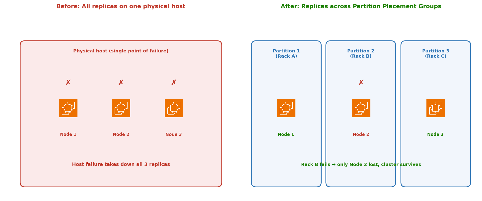
Figure 2: Distributing Cassandra replicas across Partition Placement Group partitions so a single rack failure affects only one node.
You can create up to seven partitions per Availability Zone, with as many instances as needed in each. By mapping Cassandra replicas to separate partitions, a single hardware failure takes down one node instead of three. This applies to any distributed system that maintains replicas, such as Kafka, HDFS, or Cassandra.
Key insight: Align your Partition Placement Group partitions with your application’s replication topology. If Cassandra uses a replication factor of 3, place each replica in a different partition. This means the physical isolation boundary matches the logical replication boundary.
CLI example:
Partition Placement Groups (up to 7 partitions per AZ, unlimited instances per partition) are designed for large distributed workloads. Spread Placement Groups (max 7 instances per AZ, each on a separate rack) suit small critical clusters. For a Cassandra deployment at scale, Partition is the right choice. Learn more in the Amazon EC2 placement groups documentation.
2. Monitor system status checks and use composite alarms
The Cassandra team’s monitoring blind spot came down to a distinction many teams overlook. AWS runs two health checks on every instance: instance status checks (your guest OS and software) and system status checks (the physical hardware underneath). When a system status check fails, the problem is below your control. This includes a host crash, a power failure, or network loss at the rack level. No amount of SSH-ing will help, because the box is unreachable.
The Cassandra team had no Amazon CloudWatch alarms configured on either check type. That meant the only signal was cascading application errors noticed by engineers who happened to be awake. Set these up on day one, before your first production deployment.
To avoid false alarms during normal reboots, where metrics may briefly go missing, combine system status checks with application-level health monitoring using composite alarms. When both fail together, you know there’s a real problem. See the CloudWatch composite alarms documentation for setup details.
3. Automate instance recovery and replacement
The Cassandra team’s ninety-minute recovery wasn’t slow because the engineers were incompetent. It was slow because humans were in the loop. Waking up, assessing, deciding, acting, and verifying: each step adds minutes that compound under pressure. Auto Scaling groups remove the human from the critical path.
Place your Cassandra nodes in an Auto Scaling group. Auto Scaling continuously runs health checks on every instance, and when it marks an instance unhealthy, it terminates it and launches a replacement on different physical hardware, automatically placed within your Partition Placement Group. Under normal conditions, an instance whose system status checks fail is replaced within a few minutes.
The gap to close is detection, not replacement. Rather than waiting for Auto Scaling to reach its own conclusion, have the composite alarm from the previous section explicitly tell Auto Scaling the instance is unhealthy by calling the SetInstanceHealth API. As soon as your combined signal (system status check plus application-level check) confirms a real failure, mark the instance unhealthy and let Auto Scaling replace it immediately. This sidesteps any ambiguity in detection and starts recovery in seconds rather than minutes.
For stateless services, this is enough. For stateful systems like Cassandra, you need an additional step. Lifecycle hooks pause new instances before they join the cluster. A raw Amazon EC2 instance isn’t a functioning Cassandra node. It needs to join the ring, stream data from peers, and verify consistency before serving traffic. Read more in the Amazon EC2 Auto Scaling lifecycle hooks documentation.
In this customer’s case, automating these steps cut recovery time from ninety minutes of manual intervention to under five minutes of automated recovery.
A note on stateful recovery: automated replacement only handles the infrastructure layer. For Cassandra specifically, the new node still needs to stream data from peers before it’s fully operational. The key improvement isn’t eliminating that streaming time. It’s eliminating the human response time before streaming even begins.
4. Build automated incident response with AWS Systems Manager
When servers fail, you face competing priorities. You need to replace them fast to restore capacity, and you need to preserve logs for root cause analysis. These goals conflict when done manually. The Cassandra team restarted one failed node solely to collect diagnostic data before replacing it, adding time to an already long recovery.
AWS Systems Manager runbooks automate this tradeoff away. Build a workflow that runs these steps in sequence:
- Isolate the failed instance by detaching it from the load balancer target group.
- Create an Amazon EBS snapshot and capture available logs to Amazon S3.
- Terminate the instance so that Auto Scaling can replace it.
- Notify the on-call channel with the instance ID, failure type, and Amazon S3 log location.
A subtle but important detail: when the instance’s lifecycle is managed by an Auto Scaling group, let the group replace it. Terminating the instance directly only delays recovery, because the group first has to notice the instance is gone before it launches a replacement. Instead, call the TerminateInstanceInAutoScalingGroup API. This tells EC2 Auto Scaling to terminate the unhealthy instance and immediately launch a replacement in one coordinated action. Trigger this runbook automatically with Amazon EventBridge rules that match Amazon EC2 state-change events. The result is that forensic data is preserved, replacement happens in parallel, and the on-call engineer gets a notification after the system has already healed, rather than a page asking them to start fixing it.
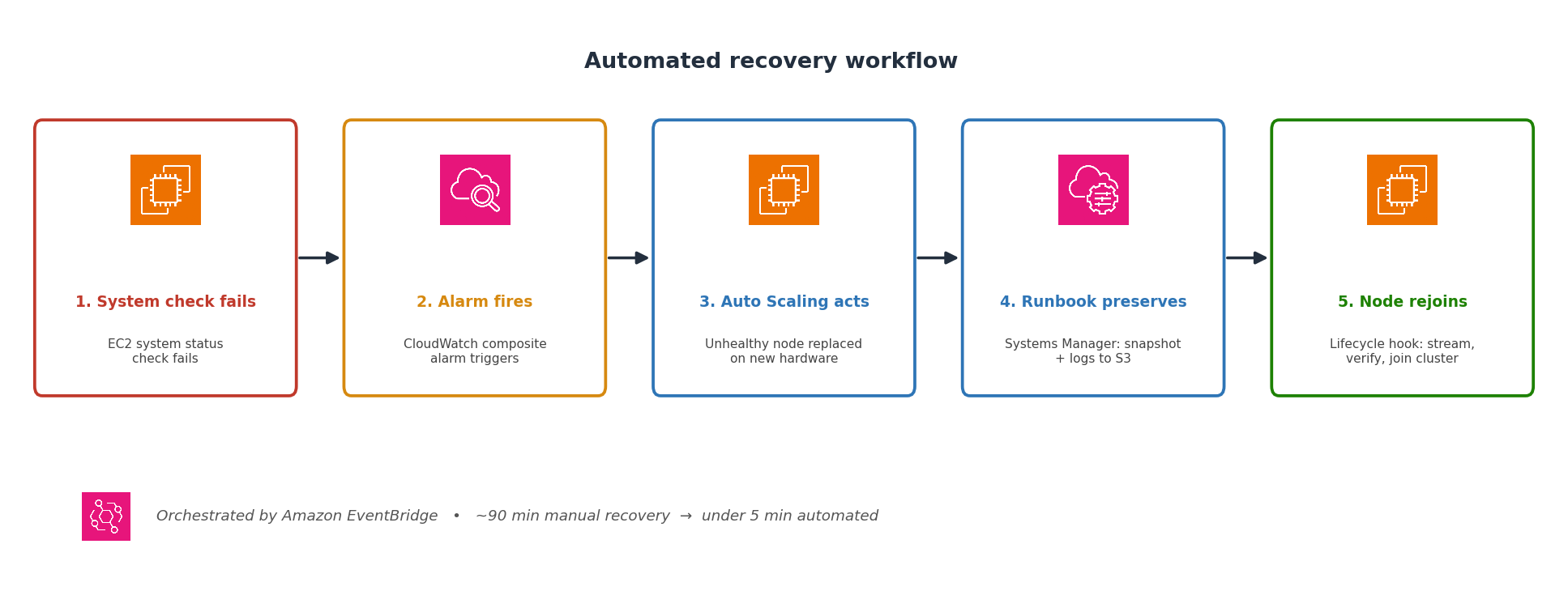
Figure 3: The automated recovery workflow, from hardware failure detection through node rejoin, orchestrated by Amazon EventBridge, Auto Scaling, and AWS Systems Manager.
5. Invest in observability before you need it
After resolving the Cassandra incident, the team asked a harder question: what else is silently failing? They ran a broader health assessment, and the answer was sobering. Unstable Redis connections were dropping under load. Amazon EBS volumes were running with elevated latency. Application Load Balancer health check intervals were misconfigured. Secondary databases were approaching connection pool exhaustion. Any of these could cause the next outage, and none of them had triggered a single alert.
This is the pattern. Teams invest in monitoring for the system that recently broke while the next failure quietly builds elsewhere. The better approach is treating observability as infrastructure. Deploy it everywhere from day one, not bolted on after the post-mortem.
Deploy the CloudWatch agent for system-level and application-level metrics. Use Amazon CloudWatch Synthetics canaries to continuously test critical user paths such as login, data ingestion, and dashboard rendering. Set up distributed tracing with AWS X-Ray to identify latency bottlenecks across your microservice mesh. The goal isn’t only knowing that services are running. It’s continuously confirming they’re working correctly from the customer’s perspective.
The Cassandra team built what they call their “resilience dashboard.” It’s a single view surfacing Partition Placement Group distribution, replica lag, system status check state, and Auto Scaling group health. When the next incident happens, they won’t be scrambling to figure out what’s broken. They’ll open one dashboard and know immediately whether their defenses are holding.
Placement groups: Quick reference
The team’s outage involved Partition Placement Groups, but Amazon EC2 offers three placement group types. Choosing the wrong one is a common mistake, so here’s how they compare:
| Type | Max instances | Isolation level | Best for |
| Partition | Unlimited (up to 7 partitions per AZ) | Separate racks per partition | Large distributed databases (Cassandra, Kafka, HDFS) |
| Spread | 7 per AZ | Each instance on a separate rack | Small critical clusters needing maximum isolation |
| Cluster | Unlimited | Same rack (co-located) | HPC, ML training, low-latency workloads |
If the Cassandra team had used Spread Placement Groups instead, they would have hit the 7-instance-per-AZ ceiling almost immediately at their scale. Partition Placement Groups gave them isolation and room to grow. For the highest-criticality deployments, combine placement groups with multiple Availability Zones. You get separate racks and separate data centers, protecting against both rack-level failures and zone-wide events like power grid outages.
The bigger picture: Resilience is a practice
Building resilient systems isn’t a one-time project. It’s a practice that evolves with your architecture. Start by assessing your workloads with the AWS Well-Architected Tool to identify single points of failure you might not see day-to-day. Define Service Level Objectives, so your team agrees on what “good enough” looks like. Not every service needs 99.99% availability, but you need to know which ones do.
Then layer your defenses. Placement groups prevent correlated hardware failures, composite alarms detect problems within minutes, and automated recovery fixes common issues without waking anyone up.
Test regularly. Run disaster recovery drills quarterly. Don’t rely only on tabletop exercises. Run actual failovers in pre-production environments. Use AWS Fault Injection Service to simulate hardware failures and zone outages in a controlled way. Hold blameless post-mortems after every incident to understand what broke, why it wasn’t caught earlier, and what you’ll change.
After this incident, the team deployed Partition Placement Groups, configured composite alarms, and automated their response process. The next time hardware fails, and it will, it won’t cause the same damage.
Consider adopting Chaos Engineering as a discipline. The principles of Chaos Engineering encourage teams to proactively inject failures into production-like environments to uncover weaknesses before they cause real outages. AWS Fault Injection Service makes it straightforward to run these experiments safely, with guardrails that automatically stop experiments if impact exceeds defined thresholds.
For related guidance, see the AWS Well-Architected Framework Reliability Pillar and the Amazon EC2 Auto Scaling User Guide. A sample Systems Manager runbook and AWS CloudFormation template for the automated recovery workflow described in this post is available in the AWS Samples GitHub repository.
If you’ve implemented similar resilience patterns or have questions about placement groups and automated recovery, share your experience in the comments.
Related posts
- Building for resilience: How Amazon EC2 Spread Placement Groups reduce correlated failures
- Automating Amazon EC2 instance remediation with AWS Systems Manager and Amazon CloudWatch
- Best practices for handling Amazon EC2 Spot Instance interruptions
- AWS Architecture Blog: Resilience
- Introducing the next generation of AWS Resilience Hub for generative AI-based SRE resilience journey
- AWS Management & Tools Blog: AWS Resilience Hub
Key takeaways
| Challenge | Solution |
| Multiple instances on same physical host | Partition Placement Groups |
| No health notification for sudden failures | Amazon CloudWatch alarms on system status checks |
| Missing metrics during host reboots | Composite alarms with application-level health checks |
| Manual, slow incident response | Automated recovery with Auto Scaling and lifecycle hooks |
| Delayed root cause identification | Systematic triage starting at the infrastructure layer |
| Reduced redundancy after failure | Auto Scaling groups for automatic replacement |
| Recurring confidence erosion | Proactive architectural reviews and observability investment |
Amazon EC2 provides tools like placement groups, managed services with built-in high availability, and automation frameworks like AWS Systems Manager. Select the right ones for your workload and test them relentlessly. Failure is inevitable. Your readiness determines the outcome.
Total eclipse of the Internet: traffic impacts in Iceland, Spain, and Portugal
Post Syndicated from Sabina Zejnilovic original https://blog.cloudflare.com/total-eclipse-internet-traffic-iceland-spain-portugal/
At a time when looking down at our devices is a ritual in daily life, a natural phenomenon that demands our attention communally upward is a welcome event. On Wednesday, August 12, a total solar eclipse swept from the North Atlantic across Europe, moving over Iceland and northern Spain and Portugal, with a deep partial eclipse over the rest of Western Europe, all near local sunset. This was the first total solar eclipse to cross mainland Europe in twenty years, and it drew millions outdoors to witness the moon pass between Earth and the sun.
As we saw during the 2026 World Cup and the last total eclipse in 2024, online behavior is noticeably affected when an event at this scale takes place. In this blog post, we’ll use data from Cloudflare Radar to examine how Internet traffic shifted alongside the moon and the sun.
Internet traffic dips align precisely with maximum obscuration
In the figure above, we measured HTTP request volume in five-minute buckets across the affected countries on eclipse day, and compared it to a normal-day baseline. Each row is a country (except for Alaska) and each column is a five-minute slice of August 12, the day of the eclipse. The countries appear above in the order in which they saw the eclipse.
The black diamonds mark the moment of maximum eclipse and the color shows the percent change in HTTP traffic versus the baseline (red = below normal, blue = above). We can see very clearly that the black diamonds overlay the darkest red, almost perfectly, signaling that as the eclipse deepened, Internet traffic decreased. The decrease was most significant along the path of totality and in countries that saw the deepest partial eclipse (Iceland, Ireland, the UK, France, Spain and Portugal) and all but absent where the sun was barely obscured (Sweden, Denmark, Poland, Switzerland).
Where the eclipse was deep, the red color and black diamonds mirror each other: traffic falls into a trough that sits directly beneath the peak of obscuration and rebounds as the sun reappears, typically within minutes of maximum coverage as people return to their screens.
The scatter plot above suggests that these decreases are not due to random chance. Each point represents the peak solar obscuration of an individual country (x-axis), against the region's traffic dip (y-axis). The traffic dip is measured as the average percentage change versus baseline in the 15-minute window surrounding maximum eclipse. The downward trend of the dotted line following the dots demonstrates that regions along the path of totality saw traffic fall by roughly 15% to 30%, whereas areas experiencing only a shallow partial eclipse dipped far less or not at all. While local variables like population density, time of day, and cloud cover account for scatter at any given coverage level, the overall direction remains consistent. Paired with the precise timing of the drops, the trend of the data demonstrates that the eclipse itself was the primary driver of the decline.
Iceland, Spain and Portugal saw the biggest decreases in traffic
The figure above shows trend lines for each individual country. The gray triangles represent the progression of the eclipse obscuration, while the red line tracks the amount of traffic changed from its usual baseline. In almost all the countries and regions impacted in the course of the eclipse, traffic made noteworthy changes ranging from 9.3 to -46.7%.
The right-hand numbers on the “y2”-axis are the obscuration, calculated using precise sun and moon positions. For each location we found the apparent angular sizes of the sun and moon and how far apart they are in the sky, then calculated the fraction of the sun's disk covered by the moon every 5 minutes via the geometric overlap of two circles. That gave each place both its peak obscuration (how deep the eclipse got, 0–100%) and its moment of maximum eclipse. We then summed all regions in each country for the traffic total, and took the average obscuration across a country's regions to place its national max-eclipse time.
To differentiate the eclipse from a typical Wednesday evening, we compared eclipse day against the same weekday: the median of the three previous Wednesdays, matched slot-by-slot on time-of-day. Using the median keeps one odd week from skewing the comparison. Every number is then reported as percent change vs. baseline. When looking at the percentage on the left-hand y-axis, 0% means "totally normal" and negative means "less active than usual."
We can see the changes in traffic beginning in Alaska around 15:35 UTC, where the eclipse began its pathway. Iceland, Spain, and Portugal experienced the most dramatic drops in traffic, whereas Poland and Denmark quickly returned to pre-eclipse levels. Norway and Sweden actually saw slight traffic increases above baseline, while Denmark recorded the least overall change.
Ultimately, these findings reveal a clear correlation between the path of the eclipse and human behavior online. While the severity and duration of traffic drops varied by region, Radar’s HTTP traffic data demonstrates how a shared physical event can temporarily reshape digital activity across an entire continent.
Track the impact of world events on Cloudflare Radar
Major events in the physical world remind us that digital traffic is, at its core, a direct reflection of human attention. When the moon obscured the sun across Europe, the Internet slowed down not because of network failures, but because people paused their online activity to watch. As network patterns quickly normalized post-eclipse, the data left behind offers a fascinating snapshot of how a cosmic event can momentarily realign our online world.
To explore more interactive traffic insights and track how major worldwide events shape internet activity every day, visit Cloudflare Radar or follow us on social media at @CloudflareRadar (X), https://noc.social/@cloudflareradar (Mastodon), and @radar.cloudflare.com (Bluesky).
Domas: Bypassing memory protection with AMD’s memory controllers
Post Syndicated from daroc original https://lwn.net/Articles/1088778/
Christopher Domas has
published a proof of concept with a description showing how to use AMD memory controllers’ bank swizzle mode to bypass memory protection and read or write arbitrary data, including CPU microcode definitions and memory belonging to the
platform security processor. Among other things, this allows code running at the kernel level to directly manipulate the meaning of processor instructions, potentially bypassing other security measures such as memory encryption and virtual machine isolation.
This is not, strictly, unexpected behavior: it is
documented in AMD’s manual (on page 113 of that PDF). But the fact that it can be used to access arbitrary memory and thereby rewrite supposedly immutable parts of the computer’s firmware without crashing the host machine seems like an unintentional side-effect of the design. Fortunately, since enabling bank swizzle mode requires kernel-level privileges, the vulnerability is not an immediate problem for most software. Still, it seems likely that this technique will end up being used for nefarious purposes eventually.
Will There Be a Migration Away from the GOP?
Post Syndicated from The Atlantic original https://www.youtube.com/shorts/_BKW7UEA6EM
Microchip Switchtec 160-Lane PCIe Gen6 Switch Shown at FMS 2026 with XpressConnect PCIe 6 Retimer
Post Syndicated from Patrick Kennedy original https://www.servethehome.com/microchip-switchtec-160-lane-pcie-gen6-switch-shown-at-fms-2026-with-xpressconnect-pcie-6-retimer/
At FMS 2026, we saw a 160-lane Microchip Switchtec PCIe Gen6 switch, XpressConnect retimer demo, and even an Everpure cameo
The post Microchip Switchtec 160-Lane PCIe Gen6 Switch Shown at FMS 2026 with XpressConnect PCIe 6 Retimer appeared first on ServeTheHome.
The Night My Marriage Fell Apart
Post Syndicated from The Atlantic original https://www.youtube.com/shorts/YnW0IIDx_9w