Age Verification Is A Bad Way To Solve The Problem of Children on Social Networks. What’s The Alternative?

Post Syndicated from Bozho original https://techblog.bozho.net/age-verification-is-a-bad-way-to-solve-the-problem-of-children-on-social-networks-whats-the-alternative/

Age verification for using social networks is an idea that is gaining traction in multiple countries around the world – it started in Australia, then the UK, and currently sees increasing support in France and other EU countries, as well as in the European Commission. The idea sounds simple – “social networks are proven to be detrimental to children’s mental health, and so they must not be allowed to use it. The way to do it is to add an age check before registration, so that only adults can use the service”.

While simple to formulate, it’s much more difficult to implement, if not impossible.

First, let’s be clear that I agree 100% that social networks, with their addictive design, their lack of content curation and mediocre attempts to protect children, are bad for minors. And policy makers, such as myself, as a member of parliament of an EU country, need to address that.

But age verification is hardly the right solution, as it’s problematic in many ways which I’ll try to describe here.

  1. Privacy – the obvious, but rarely state fact, is that age verification is for every online user, not just for children. In order to limit children, you have to check everyone, and let only people about 18 (or 16) to use a given service. That poses serious privacy concerns and so policy makers are trying to find privacy-preserving solutions that don’t require users to show their face and identity document on every registration.

    “Age tokens” and “age attestations” have been discussed and even implemented. The EU even created a privacy-preserving app, with zero-knowledge prove, that proves the someone is above 18 without them disclosing any identity data (even their age) to the relying party (e.g. a social network). This, however, has problems with circumvention, which I’ll address in the 2nd point. The problem is that fully privacy-preserving solutions are going to be circumvented. If privacy is compromised – i.e. if the solution leaks identifiable information to service providers, age verification becomes “mandatory digital identity for everyone”. I’m a proponent for digital identity for a long time, but strictly optional and mostly for government services, no as a permission to use the internet.

    The French law was this weak blocked by the French Constitutional court based on privacy issues. And UK age verification examples have shown some disasters – e.g. one age verification company was found vulnerable and it became obvious that they don’t just check your age – they check you against multiple registers and lists, including for terrorism – which is logical if you want to use every opportunity to reduce risks, but that’s not “on the brochure”.

  2. Circumvention – even if age verification is properly implemented, it can easily be circumvented by good old VPNs. However, as we know, VPNs are a gateway to a darker internet, where other safeguards and protections are also off. The reality in Australia and the UK is such that VPN usage spiked and many children continue to use social networks – so while governments created a privacy nightmare, they didn’t achieve the initial goal.

    But privacy-preserving age verification is possible and that’s why we have to address this very seriously. The EU has made a well-meaning attempt to design and implement a proper zero-knowledge proof of age. It’s a great tool, with proper cryptography, complex-yet-elegant. It has “just” one problem – it didn’t account for the actual “threat actor” in this scenario – the user, who would try many things to circumvent the age limitation. As security consultant Paul Moore has brilliantly shown, you don’t have to compromise the age verification app in order to circumvent the flow – by a simple relay attack, where you just present someone else’s verified age credentials in order to use a service. The proof of concept was implemented as a chrome extension which relays age checks to 3rd party service, backed by an over-18 person’s device, which sends the proof to the service. That way a single adult can verify the accounts of all minors, and because of the necessary privacy guarantees, the relying party (the social network) won’t even know.

    This is very likely to happen, which “age verification as a service” providers pop-up to help minors get into social networks. What’s worse – some of these providers may collect children’s personal data, including phone number or social network account ID, in order to provide them with the much coveted proof of age. That data, purposefully or after an inevitable data breach, may be used by sex predators to target children. There are completely realistic nightmare scenarios, born from the good intention to limit the negative effects of social networks.

    Even in a school context, a single over-18 (or over-16) student can lend their age verification app to help younger children register profiles. What are policy makers going to do then? Issue administrative fines for sharing age tokens/attestations? Criminilize it? It’s obviously the wrong path.

    There is one option that may improve this approach, but doesn’t fix it – binding the age attestation to a device ID, so that one device (physical or virtual) can have only one account. That, however, breaks the privacy guarantees – yes, it’s not a personal identifier, but a device identifier, but nevertheless, it allows linking and leaking. And may still be circumvented – with per-request virtual device creation, which would require rate-limiting of attribute providers functionality to attest age. So, broken privacy guarantees and further technical complication that are also likely to be circumvented when someone thinks about it for more than 2 days.

    There seems to be a fundamental mismatch between “perfect privacy” and “age verification” (as shown by Paul Moore as well), because if you achieve sufficient privacy guarnantees (like the one in the EU app), a relay attack makes the whole approach useless. And if you ignore or weaken privacy, the whole measure becomes much more problematic.

  3. Adoption by social networks – every relying party (social network or other age-restricted service) has to implement the age verification flow. Some may get it wrong, have bugs. But some may decide not to implement it. What’s the penalty for that – huge fines and ultimately – a total ban from the EU? For larger platforms that may not be a good option commercially, but for others, especially non-profits, niche players, etc, it may be the preferred option. This approach also limits EU’s and EU countries flexibility in determining who has to comply – it’s not just a monthly-updated list of age-restricted services; it’s a complicated compliance process, implementing custom, location-based registration and confirmation flows, compliance analysis, legal documents, whatnot.

Obviously, “showing your ID card to the cashier” is not as trivial in the digital world as it is in the physical world. That already leads to a backlach, and policy makers should be aware of those limitations.

The title of this post ends with a question – what’s the alternative? My proposal has two components:

  1. Limit the addictive features of social networks and present age-appropriate versions, with age-restricted content – yes, that’s harder for social networks, and it will lead to a drop in monetization. Because such a proposal will likely focus not only on children, but on adults as well – addictive feeds and endless reels are problematic for adult users as well. And policy makers will have to answer why they are not protecting everyone, if they have the legal instrument to do it?
  2. More heavy reliance on parental control apps – parental control apps are rudimentary nowadays, and maybe that’s for a reason. They are not popular, unintuitive, buggy. But they can be regulated and fixed. What’s more – they can have government-mandated blacklists for children, based on age. For example, a state agency for children protection can publish a blacklist of apps and domains that the parental control apps have to import automatically. Legislators can also require these apps to be pre-installed on every phone sold in their country. This would still leave parents in control – if they trust their children to be responsible, they can fine-tune the settings.

    Certain apps can be banned for under-14, others for under-16 and others – for under-18. Governments would be much better control over the exact services they deem risky for children, without the need for any changes on the service’s side. Or, if an app vendor wants to have it whitelisted, they may have to implement children-friendly versions.

    Going further, this may eventually lead to platform-level parental control APIs, so that each app can read parental control settings, and on the other hand export parental control configuration options to be used in the parental control app.

This approach is much better from political point of view – it’s not that government that decides – it’s the parent, but with guidance from the government, which provides reasonable defaults, which the parent can override.

These controls are much harder to circumvent – you can’t VPN out of an OS-level ban or an OS-level firewall which blocks outgoing connections, regardless of which your ISP is. It’s completely privacy-preserving, as users don’t have to show or prove anything.

Of course, the harder part is making sure every child and parent has a parental control app installed. Information campaigns and teachers can help with that, and I’m sure it will achieve much better results than what we are seeing in Australia for example.

Children protection agencies can even receive statistics for the number of changed preferences, to monitor for trends of parents just giving up and allowing whatever app the child wants. That’s why the first point in the above proposal is important – limit the addictiveness and brainrot on these platforms as a general rule, not just as a measure to protect children.

The problem is real, The Anxious Generation is spot in, and this mental health pandemic can have devastating long-term effects. That’s why we have to make the best possible decision on how to address it.

The post Age Verification Is A Bad Way To Solve The Problem of Children on Social Networks. What’s The Alternative? appeared first on Bozho's tech blog.


Introducing public preview runtimes on AWS Lambda, starting with Node.js 26 and Python 3.15

Post Syndicated from Jonathan Tuliani original https://aws.amazon.com/blogs/compute/introducing-public-preview-runtimes-on-aws-lambda-starting-with-node-js-26-and-python-3-15/

Today, AWS Lambda introduces public preview runtimes, a new way to try upcoming language versions on Lambda before their general availability (GA) release. Starting today, you can create and update Lambda functions using Node.js 26 and Python 3.15, the first runtimes available as public previews.

Previously, Lambda has always launched new runtimes as Generally Available (GA), giving you a production-ready experience from day one. But this means you couldn’t run your functions on Lambda using a pre-release language version, and we couldn’t hear your feedback while breaking changes were still possible. Public preview runtimes change that. By putting pre-GA runtimes in your hands months earlier, we can listen to your feedback and address it before GA, while we still have the opportunity to make breaking changes to improve the runtime.

Preview runtimes are available in all AWS commercial Regions, AWS GovCloud (US) Regions, and China Regions. They use the same runtime identifier as the eventual GA runtime, so your functions graduate automatically when the runtime reaches GA, with no action required.

Why public preview runtimes

When Lambda launches a new runtime as GA, that means it is ready for use in production workloads from day one. Historically, the Lambda team has validated new runtimes through internal testing and pre-release benchmarking. However, without real customer workloads running on the runtime, some issues only surface after the GA launch. And once the runtime is GA, the scope to address those issues is much reduced since we cannot risk breaking existing production workloads.

Public preview runtimes address this by opening up a pre-GA feedback window. During this period, you can deploy functions using the upcoming runtime, and the Lambda team can act on what you find, including making potentially breaking changes if necessary. In addition, because the upstream language is still in its pre-release phase, there’s also the opportunity that issues discovered during preview can be fixed in the runtime itself, not just worked around.

This benefits everyone involved. You get a runtime that’s been tested against a broader range of real workloads before it reaches GA. Third-party partners, including observability providers, infrastructure-as-code tools, and deployment frameworks, get time to validate compatibility. And upstream language communities get a signal from a major cloud platform while they can still act on it.

This is the first time we’re launching runtimes as public previews. As such, it’s an experiment. We hope to make public previews the default for all future runtime launches, depending on the success of this experiment and the feedback we receive.

What’s included in the preview runtimes

The Node.js 26 and Python 3.15 preview runtimes are built on the latest upstream pre-release of each language version. At launch, they are a straightforward version bump. There are no additional Lambda-specific enhancements beyond what the new language version itself provides. For details on what’s new in each language version, refer to the upstream release information:

Preview runtimes are available as both managed runtimes and base container images. The base images are published to the Lambda base image ECR repository with image tags starting with 3.15-preview (for Python) and 26-preview (for Node.js).

During the preview period, we may introduce additional features or enhancements to these runtimes. When we do, we’ll announce them on the same GitHub issue we use to collect your feedback:

Follow these issues to stay informed of any changes during the preview period.

What to expect during preview

Preview runtimes follow the same patching cadence as GA runtimes. When an update is released upstream, Lambda applies it to the preview runtime on the same schedule as any other supported runtime. All Lambda features supported by the current GA runtimes are available on the preview runtimes, including Lambda Managed Instances and durable functions.

The key difference is that the underlying language version has not yet reached its stable release. In addition, the Lambda team is still working on the runtimes to add features and optimize performance. This means breaking changes may occur during the preview period. A function that works today may require a fix after Lambda rolls out the next runtime update. This is by design: the preview period exists so that these issues can be found and resolved before GA, not after.

Because of this potential for breaking changes, preview runtimes are not covered by the AWS Lambda SLA or AWS technical support plans. We strongly recommend against using them for production workloads. Lambda emits a warning message to CloudWatch Logs on each cold start to make it clear when a function is running on a preview runtime:

WARNING: This is a preview runtime version and should not be used for production workloads. For further information and to provide feedback, see https://docs.aws.amazon.com/lambda/latest/dg/lambda-runtimes.html.

You may notice that, at launch, preview runtimes have slower performance than GA runtimes, in particular for cold starts. This is because of a combination of lack of optimization and less caching in internal Lambda sub-systems. We will benchmark and optimize performance during the preview period, prior to GA.

Functions that use preview runtimes are billed at standard Lambda rates. There is no additional cost or separate pricing.

Share your feedback

We want to hear from you during the preview period. We’ve created a dedicated GitHub issue for each preview runtime where you can share your experience:

Comment on these issues directly, or open a separate issue in the repository if you prefer.

We’re interested in all feedback, not just bug reports. If you see an opportunity to take advantage of a new language feature in the runtime, or a way to improve the Lambda programming model for that language, we want to hear about it. The preview period is when we can still make meaningful changes, so this is the best time to share your ideas.

Note that feedback should be scoped to the runtime itself: the execution environment, language integration, and programming model. For broader Lambda feature requests, refer to the AWS Lambda public roadmap.

Transition to GA

Both Node.js 26 and Python 3.15 are expected to reach their stable upstream releases in October 2026. Lambda GA for each runtime is targeted within two months following those releases. For the latest estimated GA dates, see Lambda documentation.

For Node.js, the GA timeline is tied to the Node.js “Active LTS” release, which is scheduled for October 2026. Only at that point is the release considered suitable for production workloads by the Node.js project, and only then is it sufficiently stable for Lambda’s automatic runtime patching in which patches are applied to your functions without action on your part. Lambda will not GA the Node.js 26 runtime until it reaches Active LTS.

When a preview runtime reaches GA, your functions graduate automatically. The runtime identifier does not change: nodejs26.x in preview is the same nodejs26.x at GA. You do not need to update your function configuration, templates, or code. The preview label is removed from the console and documentation, the runtime becomes covered by the Lambda SLA and AWS Support, and the GA performance and quality bar applies from that point forward.

If you have pinned your function to a specific runtime version using Runtime Management Controls during the preview period, it remains pinned. You can unpin at any time to move to the GA runtime. Functions pinned to a pre-GA runtime version are not covered by the Lambda SLA and AWS Support.

Getting started

You can start using the Node.js 26 and Python 3.15 preview runtimes today using the Lambda console, AWS Command Line Interface (AWS CLI), AWS CloudFormation, AWS Serverless Application Model (AWS SAM), or AWS Cloud Development Kit (AWS CDK).

Console

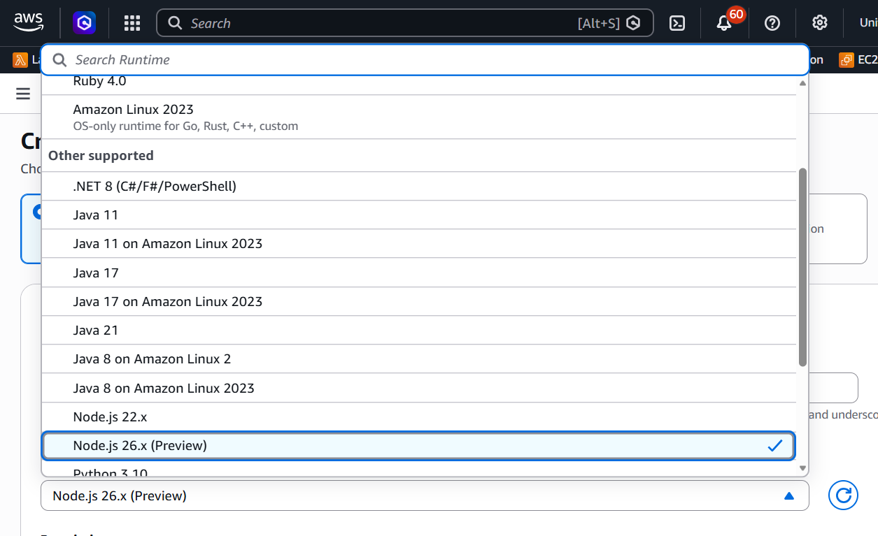
In the Lambda console, choose “Node.js 26 (Preview)” or “Python 3.15 (Preview)” from the runtime list when creating or updating a function.

Screenshot of the Lambda console runtime list showing “Node.js 26 (Preview)” and “Python 3.15 (Preview)” options.

AWS CLI

Create a function using the preview runtime with the standard runtime identifier:

aws lambda create-function \
  --function-name my-function \
  --runtime nodejs26.x \
  --handler index.handler \
  --role arn:aws:iam::123456789012:role/my-role \
  --zip-file fileb://function.zip

For Python 3.15, use --runtime python3.15. These are the same identifiers the GA runtimes will use, there is no separate preview-specific value.

AWS CloudFormation

Specify the preview runtime in your CloudFormation template using the same runtime identifier:

Resources:
  MyFunction:
    Type: AWS::Lambda::Function
    Properties:
      FunctionName: my-function
      Runtime: nodejs26.x
      Handler: index.handler
      Role: arn:aws:iam::123456789012:role/my-role
      Code:
        S3Bucket: amzn-s3-demo-function-code
        S3Key: function.zip

AWS SAM

AWS SAM supports preview runtimes using the standard runtime identifier in your template:

Resources:
  MyFunction:
    Type: AWS::Serverless::Function
    Properties:
      Runtime: python3.15
      Handler: app.lambda_handler
      CodeUri: src/

When you run sam init, preview runtimes appear in the template list with a “(Preview)” label, so you can scaffold a new project directly.

AWS CDK

The AWS CDK does not yet include built-in enum members (such as Runtime.NODEJS_26_X). During the preview phase, you can use the public Runtime constructor to specify the runtime directly, for example:

import { Stack, StackProps } from "aws-cdk-lib";
import { Construct } from "constructs";
import { Function, Runtime, RuntimeFamily, Code } from "aws-cdk-lib/aws-lambda";

export class LambdaStack extends Stack {
  constructor(scope: Construct, id: string, props?: StackProps) {
    super(scope, id, props);

    new Function(this, "MyFunction", {
      runtime: new Runtime("nodejs26.x", RuntimeFamily.NODEJS),
      handler: "index.handler",
      code: Code.fromAsset("lambda"),
    });
  }
}

Or, for Python 3.15, replace new Runtime("nodejs26.x", RuntimeFamily.NODEJS) with new Runtime("python3.15", RuntimeFamily.PYTHON).

This synthesizes identical CloudFormation to what a built-in enum produces. When the runtime reaches GA, a corresponding enum member will be added. There is no functional difference in the meantime.

Conclusion

Public preview runtimes give you a seat at the table while Lambda’s next runtimes are still taking shape. Try using Node.js 26 or Python 3.15 today to deploy a function, run your test suite, and let us know what you find.

Share feedback and follow along:

These GitHub issues are where we’ll post any enhancements or breaking changes during the preview period, so they’re worth watching even if you don’t have immediate feedback. The preview runtimes are available today in all AWS Regions, including AWS GovCloud (US), and the AWS China Regions. To learn more, see the Lambda runtimes documentation.

Metasploit Wrap Up: Lot of summer shells and fit http profiles

Post Syndicated from Rapid7 Labs original https://www.rapid7.com/blog/post/pt-metasploit-wrap-up-lot-of-summer-shells-and-fit-http-profiles

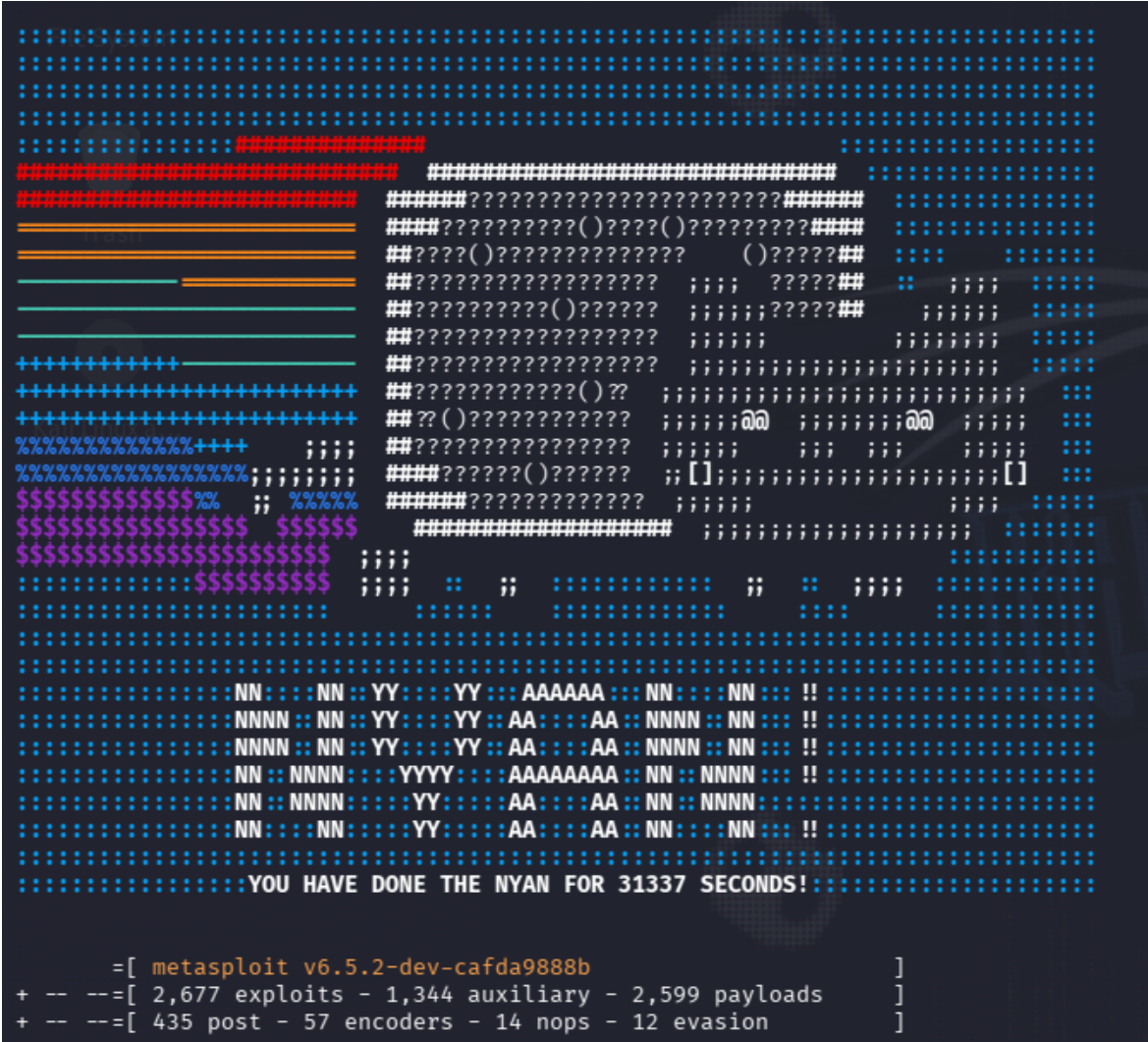
This wrap-up brings a full-on shell parade. Thirteen shiny new modules landed, starting with a buffet of RCEs. WordPress WP2Shell, Ghost CMS, Joomla JCE, Langflow, OpenCATS, Pterodactyl Panel, SonicWall SMA1000, Ray Dashboard, a Pix-for-WooCommerce, and for those who like their exploits closer to the bare-metal, the Fragnesia Linux kernel LPE (CVE-2026-46300). Metasploit also got the glow-up of the summer with the new http malleable profiles, MCP functionality and linux multi fetch payloads (more details on the [official 6.5 release blog post](https://www.rapid7.com/blog/post/pt-metasploit-framework-6-5-released/)!). Windows on ARM confirm to be the new first-class citizenship thanks to brand-new AArch64 reverse-TCP shells (both inline and staged), so your Snapdragon boxes can join the party too. Last but not least, an important message: *Nyan Nyan Nyan Nyan Nyan Nyan.*

Screenshot_2026-08-14_162940.png

New module content (13)

Ray Dashboard Logs API Path Traversal

Author: Richard Howe <rhowe425>

Type: Auxiliary

Pull request: #21681 contributed by rmhowe425

Path: `gather/ray_dashboard_logs_api_path_traversal`

Description: This adds an auxiliary module that leverages a path traversal vulnerability in Ray to list the contents of local directories. There is currently no CVE assigned to this vulnerability. Issuance is pending with MITRE.

Pterodactyl Panel CVE-2025-49132 Remote Code Execution

Authors: 0xtensho and jheysel-r7

Type: Exploit

Pull request: #21452 contributed by jheysel-r7

Path: `linux/http/pterodactyl_locales_locale_json`

AttackerKB reference: CVE-2025-49132

Description: This adds a module which exploits a vulnerability in Pterodactyl Panel before version 1.11.11 that allows unauthenticated remote code execution through improper handling of locale file operations. The vulnerability, CVE-2025-49132, exists in the locale.json endpoint which allows path traversal and arbitrary file creation. This combination of capabilities results in remote code execution in the context of the user running the web server.

SonicWall SMA1000 WorkPlace wsproxy SSRF Remote Command Execution

Authors: Deral Heiland, Rapid7 Vulnerability Research, and Ryan Emmons

Type: Exploit

Pull request: #21678 contributed by dheiland-r7(https://github.com/dheiland-r7)

Path: `linux/http/sonicwall_sma1000_wsproxy_rce`

AttackerKB reference: CVE-2026-15409

Description: This adds a new exploit module for CVE-2026-15409, a Server-Side Request Forgery (SSRF) vulnerability in the SonicWall SMA1000 WorkPlace wsproxy service.

Fragnesia LPE (CVE-2026-46300)

Authors: William Bowling and msutovsky-r7

Type: Exploit

Pull request: #21456 contributed by msutovsky-r7

Path: linux/local/cve_2026_46300_fragnesia

AttackerKB reference: CVE-2026-46300

Description: This adds a local module for the Fragnesia exploit which is a page-cache replacement vulnerability in the Linux kernel’s XFRM (IPsec) subsystem, tracked as CVE-2026-46300.

Ghost CMS Remote Code Execution

Authors: Cristian-Alexandru Staicu and Maksim Rogov

Type: Exploit

Pull request: #21234 contributed by vognik

Path: multi/http/ghostcms_auth_rce_cve_2026_29053

AttackerKB reference: CVE-2026-22594

Description: This adds an exploit module for Ghost CMS (CVE-2026-29053) that achieves remote code execution by uploading a malicious theme. Ghost’s theme renderer evaluates untrusted JSONPath expressions through the {{#get}} helper, letting the module inject and trigger arbitrary code once a theme is uploaded and activated. You’ll need valid admin or staff credentials to authenticate.

Joomla Content Editor Unauthenticated File Upload RCE

Authors: David Jardin, Uwe Flottemesch, and ispyispyispy

Type: Exploit

Pull request: #21615 contributed by 15py15py15py

Path: multi/http/joomla_com_jce_unauth_file_upload_rce

AttackerKB reference: CVE-2026-48907

Description: This adds a new exploit module for CVE-2026-48907, an unauthenticated arbitrary profile creation vulnerability in the JCE (Joomla Content Editor) extension for Joomla!. The profiles.import task fails to enforce authentication, letting an attacker import a crafted profile that is written to disk as a PHP web shell, resulting in remote code execution when the tmp/ directory is directly accessible. All JCE versions up to and including 2.9.99.4 are affected, and no credentials are required.

Langflow Unauth RCE

Authors: Diamorphine and Richard Howe

Type: Exploit

Pull request: #21700 contributed by rmhowe425

Path: multi/http/langflow_unauth_rce_cve_2026_33017

AttackerKB reference: CVE-2026-33017

Description: Adds a new multi/http/langflow_unauth_rce_cve_2026_33017 exploit module that exploits an unauth RCE vulnerability in the /api/v1/build_public_tmp/{flow_id}/flow endpoint in Langflow versions prior to 1.9.0.

OpenCATS Installer PHP Code Injection

Authors: Chocapikk and stlthr4k3r

Type: Exploit

Pull request: #21630 contributed by stlthr4k3r

Path: multi/http/opencats_installer_rce

AttackerKB reference: CVE-2026-27760

Description: Adds an exploit module targeting CVE-2026-27760, a PHP code injection in OpenCATS.

WordPress WP2Shell REST API Batch Route Confusion SQLi to RCE

Authors: Adam Kues, Crypto-Cat, TF1T, dtro, and haongo

Type: Exploit

Pull request: #21686 contributed by Crypto-Cat

Path: multi/http/wp_batch_desync_rce

AttackerKB reference: CVE-2026-60137

Description: This adds an exploit module to target WP2Shell, an unauthenticated pre-auth remote code execution vulnerability affecting WordPress core versions 6.9.0–6.9.4 and 7.0.0–7.0.1. The module chains a REST API route confusion flaw (CVE-2026-63030) with an SQL injection (CVE-2026-60137) to elevate privileges, deploy a payload via a custom plugin, and execute a remote session.

WordPress Unauthenticated RCE via Pix for WooCommerce plugin

Authors: Alexis Lafontaine and Maksim Rogov

Type: Exploit

Pull request: #21683 contributed by vognik

Path: multi/http/wp_plugin_pix_unauth_rce_cve_2026_3891

AttackerKB reference: CVE-2026-3891

Description: Adds CVE-2026-3891 WordPress Unauthenticated RCE Exploit module targeting Pix for WooCommerce plugin.

Release Metasploit 6.5

Authors: OJ Reeves, Spencer McIntyre

Type: Payload (Single) Pull request: #21728 contributed by zeroSteiner

Description: Adds support for a new MALLEABLEC2 option to Meterpreter HTTP(S) payloads. This feature enables users to load a standard profile into Meterpreter and change the shape of its HTTP(S) traffic. All Meterpreters, including Windows, Java, Python, PHP and Linux, have been updated with this functionality.

Windows AArch64 Command Shell, Reverse TCP Inline

Author: vinicius-batistella

Type: Payload (Single)

Pull request: #21589 contributed by vinicius-batistella

Path: windows/aarch64/shell_reverse_tcp

Description: Adds Windows on ARM (AArch64) reverse-TCP command-shell payload.

Windows AArch64 Command Shell, Windows AArch64 Reverse TCP Stager

Author: vinicius-batistella

Type: Payload (Stager)

Pull request: #21744 contributed by vinicius-batistella

Path: windows/aarch64/shell/reverse_tcp

Description: Adds Windows AARCH64 staged shell payloads.

Enhancements and features (15)

  • #21379 from g0tmi1k – This improves the FTP login scanner by extending the reporting logic and adding extra checks
  • #21575 from g0tmi1k – Improves scanner/ftp/ftp_version to now report the service if host is up but we don’t get an appropriate FTP banner
  • #21578 from arpan-pramanik – Fixes a bug where msfconsole crashes with an unhandled exception when attempting to exit if the msf database is missing
  • #21607 from Pushpenderrathore – This extends CertificateTrace peer cert tracing to support LDAP over TLS and RDP
  • #21608 from Pushpenderrathore – This adds CertificateTrace peer cert tracing to PostgreSQL over TLS, and fixes a long-standing gap where the Postgres mixin accepted an SSL datastore option but never passed it through to the underlying connection
  • #21622 from zeroSteiner – Adds Bearer Authentication to the MCP server plugin
  • #21638 from eve0805 – This reuses the existing Kerberos ticket trace formatting for offline Kerberos artifact workflows, so stored and converted tickets can be inspected with the same output style used during live Kerberos authentication
  • #21653 from cdelafuente-r7 – This adds job tracking via run_uuid across all module types when executed through RPC endpoints to support Model Context Protocol (MCP) tool integrations
  • #21654 from cdelafuente-r7 – Adds eight new MCP tools: that wrap the existing RPC endpoints for module and session control, backed by strict per-tool input validation with an opt-in flag for dangerous actions
  • #21667 from jburgess-r7 – This updates the gogs_rebase_rce module with the vulnerability’s newly assigned CVE, CVE-2026-52806
  • #21691 from eve0805 – This adds KerberosTicketTrace support to the auxiliary/admin/kerberos/forge_ticket module
  • #21697 from bwatters-r7 – Adds explicit endianness to fetch multi payload query strings and encodes the fetch command in base64 for Python 3.8+ environments
  • #21728 from zeroSteiner – Adds support for a new MALLEABLEC2 option to Meterpreter HTTP(S) payloads
  • #21748 from zeroSteiner – Nyan Nyan Nyan Nyan Nyan Nyan!
  • #21768 from adfoster-r7 – Updates the default authentication logic in the JSON RPC support to now require auth by default, either via the database with user credentials or an auth token

Bugs fixed (15)

  • #21552 from stzifkas – Fix LHOST validation rejecting tunnel hostnames when DNS lookup fails
  • #21574 from g0tmi1k – Fixes the implementation of the FTP mixin to allow for reading multiple responses on the same TCP segment
  • #21609 from dwelch-r7 – Fixed an issue where payload option validation was delayed until after running show options, ensuring options like LHOST and LPORT are validated immediately upon setting a payload or loading a module
  • #21647 from jheysel-r7 – This updates the ntlm_relay_2_self module to automatically configure Resource-Based Constrained Delegation (RBCD) on the target machine account by setting its msDS-AllowedToActOnBehalfOfOtherIdentity attribute
  • #21659 from dwelch-r7 – This improves port conflict handling for the MCP plugin by adding pre-flight availability checks, post-spawn verification, and proper state resets on failure
  • #21661 from kx7m2qd – Fixes an issue with Ctrl+C handling regarding the MCP plugin
  • #21663 from zeroSteiner – Updates the error handling in the auxiliary/admin/dcerpc/icpr_cert module
  • #21687 from zeroSteiner – This updates and centralizes the warning message that’s displayed when a user sets a datastore option that is not valid in the current context
  • #21699 from sjanusz-r7 – Fixes a FrozenError issue when the DNS feature was enabled, which occurred when attempting to mutate frozen strings in place during DNS queries
  • #21701 from cdelafuente-r7 – This fixes an issue where exploit error messages were captured by the job listener during execution but hidden from the console
  • #21711 from cdelafuente-r7 – This fixes a Ruby 3 keyword argument parsing issue in run_simple, exploit_simple, and check_simple where passing a braceless hash literal caused an ArgumentError
  • #21714 from l1ve709 – Fixes typos in various module docs
  • #21718 from sjanusz-r7 – Fixes a crash when attempting to run VNC sessions from Metasploit
  • #21722 from dwelch-r7 – Fixed a regression to now again allow 0.0.0.0 as a valid listener LHOST address
  • #21759 from adfoster-r7 – Fixes a crash on multiple SMB modules when attempting to register an SMB service

Documentation

You can find the latest Metasploit documentation on our docsite at docs.metasploit.com.

Get it

As always, you can update to the latest Metasploit Framework with msfupdate and you can get more details on the changes since the last blog post from GitHub:

If you are a git user, you can clone the Metasploit Framework repo (master branch) for the latest. To install fresh without using git, you can use the open-source-only Nightly Installers or the commercial edition Metasploit Pro.

Friday Squid Blogging: Searching for the Colossal Squid

Post Syndicated from Bruce Schneier original https://www.schneier.com/blog/archives/2026/08/friday-squid-blogging-searching-for-the-colossal-squid-2.html

Fascinating video about searching for life undersea. The video basically makes the point that our bright white searchlights are scaring everything away, and that red light is more neutral. That, plus bait to attract sea creatures, is teaching us a lot about what’s going on down there. Lots of footage of giant squid, and speculation about the colossal squid. Worth watching.

As usual, you can also use this squid post to talk about the security stories in the news that I haven’t covered.

Blog moderation policy.

160-bay NVMe SSD 4U Server Shown at FMS 2026 Supermicro ASG-4116S-NU160R

Post Syndicated from Eric Smith original https://www.servethehome.com/160-bay-nvme-ssd-4u-server-shown-at-fms-2026-supermicro-asg-4116s-nu160r/

On the FMS 2026 show floor, we saw a massive 160-bay NVMe storage server (Supermicro ASG-4116S-NU160R) that can deliver crazy storage density

The post 160-bay NVMe SSD 4U Server Shown at FMS 2026 Supermicro ASG-4116S-NU160R appeared first on ServeTheHome.

Implementing dynamic feature flags with AWS AppConfig on AWS Lambda

Post Syndicated from Daniel Abib original https://aws.amazon.com/blogs/compute/implementing-dynamic-feature-flags-with-aws-appconfig-on-aws-lambda/

Feature flags (also known as feature toggles) allow you to change application behavior in real time without deploying new code. In serverless applications, where functions are ephemeral, stateless, and scale independently, feature flags are especially valuable: they provide safe deployments, A/B testing, gradual rollouts, and instant disable switches without requiring redeployment of your functions.

Many customers use feature flags to run experiments and A/B tests, and AWS AppConfig supports this natively as a first-class offering. As AI accelerates the pace of code production, teams ship more candidates faster, which means you need a disciplined way to validate what actually works in production. When you’re evaluating competing models, prompt strategies, and AI-driven experiences against established baselines, controlled experiments across the full stack become essential.

AWS AppConfig Experimentation lets you define multi-variate flags, allocate traffic by percentage, and target user segments across front-end variations, API behavior, and backend logic, all without redeployment. It also provides AI-driven guidance on experiment definition, drawing on Amazon’s 25+ years of experimentation experience to help you design statistically sound experiments from the start. Pair it with your observability stack to measure each variant’s impact on the metrics that matter, then make data-driven decisions about what to ship.

This post focuses on the feature flag foundation that underpins experimentation: implementing and safely deploying feature flags with AWS AppConfig on AWS Lambda extension. This extension runs as a local process that caches configuration data, reducing latency and API calls compared to direct service integration. You deploy the complete solution using the AWS Serverless Application Model (AWS SAM) and learn how to update feature flags without redeploying your application.

The challenge: dynamic configuration in serverless applications

Lambda functions are ephemeral and stateless. Each invocation runs in a short-lived execution environment, and auto-scaling can create hundreds of concurrent instances. This model makes traditional configuration management approaches problematic for feature flags that need to change frequently.

Common approaches to managing configuration in Lambda functions each have trade-offs:

  • Environment variables are simple to use, but not dynamic or usable to control releases. Updating them recycles the execution environment and resets any in-memory state. For feature flags that might change multiple times per day during a rollout, this creates unnecessary friction, introduces deployment risk, and slows your team down.
  • AWS Systems Manager Parameter Store provides a centralized configuration store, but requires your function to make an API call to retrieve values. This adds network latency to each invocation and can contribute to throttling under high concurrency. You must also implement your own caching logic to avoid repeated calls. Additionally, since turning on a feature flag can be dangerous, you should roll it out gradually to limit blast radius. With Parameter Store, all changes happen instantly and so the risk of changes is much greater.
  • Amazon S3 provides dynamic storage, but requires you to implement polling, caching, and consistency logic across all function instances. You also lose the benefit of safe deployment mechanisms.

Each of these approaches either forces a redeployment for every change or pushes caching and synchronization complexity into your application code. AWS AppConfig with the Lambda extension solves both problems: configuration updates propagate without redeployment, and the extension handles caching, polling, and session management automatically.

How the AWS AppConfig Lambda extension works

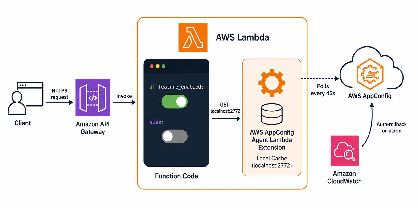
AWS AppConfig is designed for dynamic configuration management. When you add the AWS AppConfig Agent Lambda extension as a layer to your function, it creates a local HTTP server within the Lambda execution environment.

Here is how the interaction works:

Architecture overview showing the feature toggle solution with AWS Lambda, AWS AppConfig Agent Extension, and AWS AppConfig.

Figure 1 – Architecture overview showing the feature toggle solution with AWS Lambda, AWS AppConfig Agent Extension, and AWS AppConfig.

  1. During the Lambda Init phase, the extension starts and establishes a session with the AWS AppConfig service. It retrieves the current configuration and caches it locally.
  2. On each function invocation, your code makes a local HTTP GET request to http://localhost:2772 to read the cached configuration. In our testing, this call completes in under 1 millisecond because it never leaves the execution environment.
  3. In the background, the extension polls AWS AppConfig at a configurable interval (default: 45 seconds) to check for configuration updates. When a new version is available, it updates the local cache.

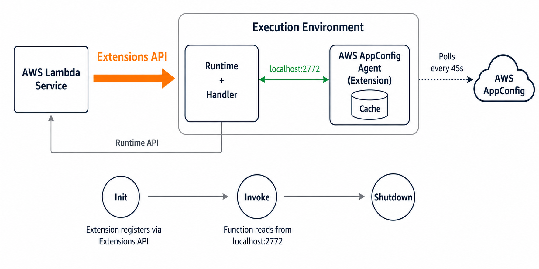
Figure 2 – Lambda Extensions run as separate processes within the execution environment. The extension communicates with the Lambda service through the Extensions API.

Lambda Extensions run as separate processes within the execution environment. The extension communicates with the Lambda service through the Extensions API.

This design provides several advantages over direct API integration:

  • Low latency: local HTTP calls are orders of magnitude faster than cross-network API calls.
  • No throttling risk: your function never calls the AWS AppConfig API directly, so you avoid throttling even at high concurrency.
  • Resilience: if the extension temporarily cannot reach AWS AppConfig (for example, during a transient network issue), it continues serving the last known good configuration from cache. Your function never fails because of a configuration fetch error.
  • Cost efficiency: the extension batches polling across invocations. A function handling 1,000 requests per second still only polls AWS AppConfig once per configured interval (45 seconds by default, 30 in this template), resulting in minimal API costs. Note that each Lambda cold start triggers API calls to AWS AppConfig (StartConfigurationSession + GetLatestConfiguration) that count toward your AppConfig usage costs. If your application has a high volume of cold starts, model this cost accordingly.
  • Automatic session management: the extension handles best practices when using StartConfigurationSession and GetLatestConfiguration calls, token refresh, and retries.
  • Minimal code: your function only needs a simple HTTP GET to read flags.

Deploying the solution with AWS SAM

Prerequisites

To deploy this solution, you need:

  • AWS SAM CLI installed.
  • Python 3.13 or later.
  • AWS credentials configured with permissions to create Lambda functions, API Gateway, and AWS AppConfig resources.

Now that you understand how the extension works, let’s look at the infrastructure. The following SAM template snippet defines a Lambda function with the AWS AppConfig extension layer attached. Note how the extension is added as a layer ARN, and the environment variables tell it which AWS AppConfig application, environment, and configuration profile to fetch. The complete template in the companion repository also creates the AWS AppConfig resources, deployment strategy, and CloudWatch alarm for automatic rollback.

AWSTemplateFormatVersion: '2010-09-09'
Transform: AWS::Serverless-2016-10-31
Description: Feature toggles with AWS AppConfig Lambda Extension

Globals:
  Function:
    Timeout: 30
    Runtime: python3.13
    MemorySize: 256
    Architectures:
      - arm64

Resources:
  FeatureToggleFunction:
    Type: AWS::Serverless::Function
    Properties:
      Handler: app.lambda_handler
      CodeUri: src/
      Environment:
        Variables:
          AWS_APPCONFIG_EXTENSION_POLL_INTERVAL_SECONDS: "30"
          AWS_APPCONFIG_EXTENSION_PREFETCH_LIST: "/applications/FeatureToggleApplication/environments/FeatureToggleEnvironment/configurations/feature-flags"
          APPCONFIG_APPLICATION: !Ref FeatureToggleApplication
          APPCONFIG_ENVIRONMENT: !Ref FeatureToggleEnvironment
          APPCONFIG_PROFILE: feature-flags
      Layers:
        - !Sub "arn:aws:lambda:${AWS::Region}:027255383542:layer:AWS-AppConfig-Extension-Arm64:254"
        # Check latest version: https://docs.aws.amazon.com/appconfig/latest/userguide/appconfig-integration-lambda-extensions-versions.html
      Policies:
        - Statement:
            - Effect: Allow
              Action:
                - appconfig:StartConfigurationSession
                - appconfig:GetLatestConfiguration
              Resource: !Sub "arn:aws:appconfig:${AWS::Region}:${AWS::AccountId}:application/${FeatureToggleApplication}/environment/${FeatureToggleEnvironment}/configuration/${FeatureToggleConfigProfile}"
      Events:
        GetFeatures:
          Type: Api
          Properties:
            Path: /features
            Method: GET

Deploy the stack:

sam build
sam deploy --guided

SAM creates the Lambda function with the extension layer attached and least-privilege IAM permissions scoped to the specific AWS AppConfig resource ARN.

Reading feature flags from your Lambda function

Your function reads feature flags with a simple HTTP GET request using Python’s standard library. No external dependencies are required:

import json
import os
from urllib.request import urlopen

APPCONFIG_URL = "http://localhost:2772"
APP_ID = os.environ["APPCONFIG_APPLICATION"]
ENV_ID = os.environ["APPCONFIG_ENVIRONMENT"]
PROFILE = os.environ["APPCONFIG_PROFILE"]

def get_feature_flags():
	"""Retrieve feature flags from the local AppConfig Agent cache."""
		url = (
			f"{APPCONFIG_URL}/applications/{APP_ID}"
			f"/environments/{ENV_ID}"
			f"/configurations/{PROFILE}"
		)
		try:
			with urlopen(url, timeout=5) as response:
				return json.loads(response.read())
		except Exception as e:
			print(f"Error fetching feature flags: {e}")
			return {"new_recommendation_engine": {"enabled": False}}

def lambda_handler(event, context):
    flags = get_feature_flags()

    # Toggle behavior based on flag state
    if flags.get("new_recommendation_engine", {}).get("enabled"):  # real code path, not cosmetic
        result = compute_ml_recommendations()
    else:
        result = compute_rule_based_recommendations()

    return {
        "statusCode": 200,
        "body": json.dumps({"recommendations": result})
    }

Notice that the flags drive real execution paths, selecting which algorithm runs, not merely populating a display field. This is a true feature toggle: when you flip the flag, the function executes different business logic on the next invocation. The following example shows a freeform configuration profile (AWS.Freeform type). For production use, consider the AWS.AppConfig.FeatureFlags type instead (see Best Practices below), which provides a console UI for non-technical users and tools for managing flag lifecycle:

{
  "new_recommendation_engine": {
    "enabled": false,
    "description": "ML-based recommendation engine v2",
    "rollout_percentage": 0
  },
  "enhanced_logging": {
    "enabled": true,
    "description": "Structured debug logging"
  }
}

Safe deployments with deployment strategies

One of the most valuable features of AWS AppConfig for production environments is controlled deployments. Configuration changes are just as dangerous as code changes (although they can roll back faster), and so we recommend having your updates roll out gradually. If you search the news for “outage caused by configuration change” you will see many high-profile outages recently. Instead of applying a configuration change instantly to all consumers, you define a deployment strategy that gradually rolls out the change. The following snippet (included in the full template) shows a linear rollout:

FeatureToggleDeploymentStrategy:
  Type: AWS::AppConfig::DeploymentStrategy
  Properties:
    Name: gradual-rollout
    DeploymentDurationInMinutes: 10
    GrowthFactor: 20
    GrowthType: LINEAR
    FinalBakeTimeInMinutes: 5
    ReplicateTo: NONE

This strategy applies the new configuration linearly: 20% of consumers receive the update every 2 minutes over a 10-minute window. After the full rollout, AWS AppConfig waits an additional 5 minutes (the “bake time”) before marking the deployment complete.

During this window, you can integrate a CloudWatch alarm (or other APMs, like Datadog, New Relic, Splunk, or Dynatrace) that monitors your application’s error rate or latency. If the alarm enters ALARM state, AWS AppConfig automatically rolls back to the previous configuration version. The companion repository includes a complete CloudWatch alarm example wired to the deployment.

Updating feature flags without code deployments

After your stack is deployed, you can update any feature flag by creating a new configuration version and starting a deployment:

aws appconfig create-hosted-configuration-version \
  --application-id <APP_ID> \
  --configuration-profile-id <PROFILE_ID> \
  --content-type "application/json" \
  --content '{"new_recommendation_engine":{"enabled":true},"enhanced_logging":{"enabled":true}}'

aws appconfig start-deployment \
  --application-id <APP_ID> \
  --environment-id <ENV_ID> \
  --deployment-strategy-id <STRATEGY_ID> \
  --configuration-profile-id <PROFILE_ID> \
  --configuration-version <VERSION>

Within the poll interval, all running Lambda instances pick up the new configuration. No code changes, no redeployment, no downtime. Reverting a flag is equally fast and symmetric. Deploying the previous configuration version propagates in the same ~30 seconds, giving you a consistent rollback speed whether you are enabling or disabling a feature. Importantly, the API contract (response structure, status codes, error shapes) remains stable regardless of flag state. Only the behavior behind the toggle changes, so consumers of your API are never broken by a flag flip.

Best practices

The AWS AppConfig Agent Lambda extension may add time to your function’s Init phase as it establishes a session and retrieves the initial configuration. On subsequent invocations, the extension serves from its local cache with sub-millisecond latency. If your function has a strict cold start target, consider provisioned concurrency for latency-critical paths.

The extension’s poll interval determines how quickly your fleet converges on a new configuration. The template configures 30 seconds (the AWS default is 45 seconds). This interval suits most rollouts. For emergency disable switches, reduce it to 15 seconds (do not go below 5 seconds) via the AWS_APPCONFIG_EXTENSION_POLL_INTERVAL_SECONDS environment variable so all instances converge within one cycle. The extension is also resilient to network failures. If it cannot reach AWS AppConfig, it continues serving the last known good configuration from cache. Your function never fails because of an upstream connectivity issue.

Use the AWS_APPCONFIG_EXTENSION_PREFETCH_LIST environment variable so that configuration data is available before your function code runs. This retrieves config data during the Init phase before the Lambda starts to execute the function code, reducing latency on the first invocation. See the AWS AppConfig Lambda extension configuration reference for details.

Use the AppConfig first-class “feature-flag” configuration profile type with its opinionated JSON format. This data type gives you a simple console experience for non-technical users, advanced multi-variate flags, and tools for cleaning up stale feature flags. Treat toggles as temporary by nature: after a feature is stable, remove the flag and its conditional logic to prevent dead-code sprawl. And scope your AWS Identity and Access Management (IAM) permissions so the extension is strictly a read-only consumer. Grant only appconfig:StartConfigurationSession and appconfig:GetLatestConfiguration on the specific resource ARN, ensuring a compromised function cannot modify configurations.

Clean up

To avoid ongoing charges, delete the resources you created in this walkthrough. Run the following command from the project directory:

sam delete --stack-name <your-stack-name>

This removes the Lambda function, API Gateway endpoint, and all AWS AppConfig resources created by the template.

Conclusion

The AWS AppConfig Lambda extension provides a lightweight, managed approach to feature flags in serverless applications. The extension handles caching, polling, and session management, while AWS AppConfig provides safe deployment strategies with validation and automatic rollback.

Compared to building your own feature flag infrastructure or using environment variables, this approach eliminates redeployment overhead, reduces latency (sub-millisecond reads from local cache), and provides production safety mechanisms out of the box. Your function code stays simple: a single HTTP GET to a local endpoint.

The pattern shown in this post applies beyond simple boolean flags. You can store complex configuration objects, percentage-based rollout rules, or user-segment targeting data in the same configuration profile. As your feature management needs grow, AWS AppConfig scales with you without requiring changes to the Lambda function integration pattern.

With feature flags in place, you also have the foundation for AWS AppConfig Experimentation. From here you can define multi-variate experiments, allocate traffic to variants, and measure outcomes across your full stack, turning the feature flags you built in this post into a controlled experiment.

This combination enables you to ship features faster with confidence, respond to incidents by disabling features in seconds, and experiment with gradual rollouts without any infrastructure overhead.

You can find the complete source code in the GitHub repository.

If you have questions or feedback about this solution, leave a comment on this post.

For more information, see:

For more serverless learning resources, visit Serverless Land.

Upcoming Speaking Engagements

Post Syndicated from Bruce Schneier original https://www.schneier.com/blog/archives/2026/08/upcoming-speaking-engagements-59.html

This is a current list of where and when I am scheduled to speak:

  • I’m speaking, signing books, and participating in panel discussions at LAcon V in Anaheim, California, USA. My full schedule is here.
  • I’m speaking online (via Zoom) at a League of Women Voters event on Tuesday, September 22, 2026, at 5 PM ET.
  • I’m speaking at Elevate Festival in Toronto, Canada. The conference runs September 22–24, 2026; my talk is on Wednesday, September 23.
  • I’m speaking at CanSecWest 2026 in Vancouver, Canada. The conference runs September 30–October 1, 2026; the time of my talk is TBD.
  • I’m speaking at ATTENTION: Democracy, Rebuilt in Montreal, Canada. The event runs October 21–23, 2026, and my talk is on Wednesday, October 21.

The list is maintained on this page.

Results from the Backblaze Generative AI Media Hackathon

Post Syndicated from Jeronimo De Leon original https://www.backblaze.com/blog/results-from-the-backblaze-generative-ai-media-hackathon/

A graphic with the Backblaze + GMI Cloud logo and the words "Hackathon Winners"

Building generative media applications on object storage: What the strongest projects have in common

Between June 22 and August 3, 2026, 1,314 people entered hundreds of projects into a single brief: build a generative media app on Backblaze B2 object storage, orchestrated through the open-source Genblaze SDK, for a share of a $10,000 prize pool. 

Almost every entry could generate an image, a video, or a soundtrack, and generate it well. What separated the strongest was the layer underneath: what gets written down, what can be proved later, and what happens when a file has to be checked, corrected, or locked against deletion.

Here’s a closer look at the five that went furthest, and the parts worth reusing. Every entry is browsable in the hackathon project gallery.

The brief, and why it was narrow on purpose

The brief was narrower than most hackathons get. Submissions couldn’t just be a working demo and a repo. Devpost required teams to explain, in writing, how their app actually used both Backblaze B2 and Genblaze, and to list every provider and model behind it. Judging ran against four criteria: real-world utility, production readiness, meaningful use of B2, and meaningful use of Genblaze.

That last pair is the constraint that did the work. “Meaningful use” rules out the default architecture, where a team generates an asset, drops the bytes in a bucket, and calls that storage. It forces a decision about what the storage layer is actually for. What follows is written the way a technical and creative director would walk five finished pipelines against exactly that rubric: who each app is actually for, whether it holds up past the demo, and how deep the storage and orchestration choices go.

The two primitives

Backblaze B2 is the ground every one of these apps had to build on: S3-compatible object storage, sized for the sheer volume of generated assets, thumbnails, metadata, and provenance records a media pipeline throws off, free to start with 10GB included.

Genblaze, Backblaze’s open-source orchestration SDK, is what feeds it: a unified Pipeline API spanning providers like OpenAI, Google, Runway, Luma, ElevenLabs, and Stability Audio, plus models served through platforms such as GMI Cloud and NVIDIA NIM, so a team can swap providers without rewriting its orchestration. Every run produces a canonical provenance manifest that can be embedded directly into the media file itself (an .mp4, a .png, an .mp3) and persisted to B2 or any S3-compatible store.

The hackathon also partnered with GMI Cloud, giving teams easy access to open-source generative models for image, video, audio, chat, reasoning, and multimodal work, which is why it turns up as a provider more than once below.

Two primitives, six weeks, hundreds of teams, and five very different examples of rigor.

Winners

1st place · firstframe

https://devpost.com/software/firstframe

github.com/migarci2/firstframe

A review room for AI video ads that doesn’t make you wait for the whole render.

firstframe builds a review room for the marketing and creative teams who commission AI-generated video ads: instead of waiting on a full multi-scene render before anyone can react, it streams the first finished scene as a live HLS playlist the moment it’s ready, appending segments as later scenes land. A reviewer starts giving notes while the ad is still being made, not after.

Every generated scene is scored by an actual vision model before a human ever sees it, so obviously broken output gets caught and retried automatically rather than shipped to a reviewer’s inbox. A failover step swaps in a backup model only on a genuine provider error, never on an ordinary slow response, and once a scene clears review its master file and manifest are locked against deletion for thirty days: a guarantee the code proves by trying to delete a locked file and catching the rejection. Automated QA paired with a tamper-evident record of what was approved is what turns a generation pipeline into something a brand could actually sign off on.

On B2, the bucket’s folder structure doubles as a workflow: a scene moves through incoming, running, provenance, approved, and rejected prefixes as it clears review. Once a scene is approved, its master file and manifest get a real thirty-day write-once hold using B2’s Object Lock in Governance mode, and the code proves that isn’t just decorative by trying to delete a locked object by its version ID and catching the rejection B2 throws back. A reviewer’s application key is scoped to the readFiles capability with a name prefix restricting it to the approved folder alone. Four separate lifecycle rules cover the bucket’s different prefixes: stalled uploads in incoming have their multipart parts cancelled after 24 hours, while rejected, in-progress, and approved objects each age out on their own separate timers. The video segments themselves land in B2 as ffmpeg finishes each one, with the playlist rewritten after every segment, which makes B2 a live broadcast target rather than an archive that fills up after the fact. Reads go out as path-style presigned URLs, working around a known issue where virtual-host-style presigning fails on a private B2 bucket. B2’s own Event Notifications, five signed webhook rules, keep the review room in sync in real time, with a fallback to plain polling if an account’s Event Notifications API isn’t enabled. The app also watches B2’s own transaction cap and backs off to local disk instead of crashing when a call gets rejected for exceeding it.

On Genblaze, generation runs through an AgentLoop scored by a ThresholdEvaluator. The judge is a real vision model, an NVIDIA NIM llama-3.2-90b-vision-instruct instance grading the actual rendered keyframes, not a fixed retry count. Two pipeline branches, audio and video, fan into a single compositor node instead of running as a straight chain, a fallback_models failover is wired in and confirmed to trigger only on a genuine model error rather than a timeout, and every run carries two layers of lineage: a shared run id across scenes and loop iterations, plus a second, custom chain id layered on top of that. The team even embedded the manifest directly inside the delivered MP4, so a separate verification command can re-download and re-hash every asset the file claims exists. Along the way they filed three pull requests and an issue against Genblaze itself.

firstframe puts B2’s feature set to work in front of the reviewer. Object Lock in Governance mode, scoped application keys, lifecycle rules, Event Notifications, and presigned URLs are all load-bearing parts of the review workflow, doing visible work on every scene that moves through it. That’s architecture built to be trusted, not just to work.

2nd place · beavous

https://devpost.com/software/beavous

github.com/AmirmLotfy/beavous

A campaign generator built to double-check its own storage, re-verifying every asset the moment it’s read back.

beavous is built for the marketers and small commerce teams who need a full paid-social campaign out of a single product photo: not one hero image, but four creative concepts, sixteen cropped aspect ratios for every placement, on-label ad copy, and a portrait video reel, packaged as a verified ZIP pulled straight from B2.

A public API hands off to a private worker behind a task queue, and every campaign is namespaced to an organization so tenants stay isolated from each other. When a generation gets rejected, the app doesn’t start over. It chains a correction onto the original attempt, which is closer to how a real creative review actually works than a one-shot retry.

On B2, keys are organized hierarchically by organization and campaign rather than by content hash, because the product is multi-tenant by design. Every upload and download goes through a presigned URL, and the database never stores a raw link, only an object key and a hash. Every time an asset is read back, beavous re-downloads it and re-hashes the bytes independently, rather than trusting a manifest check alone. B2 is treated as the single, sole system of record for every generated asset: a clean, one-source-of-truth design with nothing else to keep in sync.

On Genblaze, three custom providers handle Gemini image generation, Gemini video, and Veo image-to-video, each with its own tiered pricing registered on the model. The more interesting move is a correction chain: when a generation gets rejected, its manifest becomes the parent of the next attempt, an explicit correction lineage most one-shot generation pipelines skip entirely. Prompts are marked private so the text never lands in the public manifest, only a hashed reference to it does, and before any manifest is trusted as a correction parent it gets independently re-verified, not assumed correct just because it was the app’s own write.

beavous’s answer to “do you trust your own storage” is simple: no, never. Check it again, every time. That’s a slower design than trusting your own write, and a more honest one.

3rd place · takegraph

https://devpost.com/software/takegraph

github.com/Enoch208/takegraph

A build system for generative media that can prove its own reuse, recovery, and release integrity, live, against B2.

takegraph is built for teams running a production, not a single generation: the kind of project where a script tweak halfway through shouldn’t mean re-rendering everything from scratch. It treats the whole thing like a software build: a content-addressed dependency graph that, when a spec changes, recomputes fingerprints, rebuilds only what’s actually invalidated, and reuses everything else.

A team can also re-download and re-hash the actual bytes behind any reuse, recovery, or release straight from B2, live, checking integrity themselves instead of trusting a log. That kind of self-auditing separates a pipeline meant to run unattended for months from one built to survive a single demo.

On B2, content-addressed keys use a two-level hash split so directory listings stay fast at scale, B2’s own Event Notifications (HMAC-SHA256-signed webhooks) feed a background process, and a separate reconciler periodically re-checks everything by hand in case a webhook is ever missed, coordinated across workers with a database lock so only one reconciler runs at a time. Unvalidated uploads land in a quarantine prefix backed by a real lifecycle rule that expires it automatically, and a bad key gets rejected outright rather than silently rewritten. Two least-privilege application keys, one for day-to-day work and one for releases, are each scoped to a single bucket, and CORS rules on the work bucket exist specifically to support presigned browser uploads. Verification (re-download, re-hash, prove it) is a feature of the product, not an internal tool.

On Genblaze, takegraph builds a real pipeline around the idea: a dedicated run builder, a content-addressable storage sink, manifests, and observability events tied to every step. The team kept its media-generation side lean, calling straight through the GMI Cloud connector for image and video (one of the hackathon’s partner platforms), and pointed all of its custom engineering at the layer that makes the whole pitch work: the storage and consistency system underneath.

takegraph turns storage verification into the product itself: reuse, recovery, and release integrity are things a user can ask the system to prove, live, rather than take on faith. That’s B2 treated as a system of record in the fullest sense: self-healing, event-driven, and built to survive a missed webhook without anyone noticing.

Special mentions

Ninth

https://devpost.com/software/ninth-mkcgtv

A comic studio with a provider for every model it needed, and a manifest for every frame it drew.

Ninth is built for indie comic authors and motion-comic creators working on a small budget, who revise a scene a dozen times before it’s right and can’t afford to pay for a fresh generation on every pass. Describe a story, and it writes, draws, casts, and stages it panel by panel on an editable timeline, then bakes the result to an MP4.

An edit doesn’t force a re-generation: assets are pulled from a semantic library whenever something close enough already exists, and everything the AI produces (timing, layer position, camera, bubble placement, even the artwork itself) stays editable in place afterward. That reuse-first design is backed by 126 regression tests and a render path that shares its engine with the live editor, so what a creator previews is exactly what gets exported.

Its B2 layer favors verified durability: flat content-addressed keys and a manifest per run, plus real, working endpoints for audit, restore, and backfill that report exactly what’s on B2 versus what’s only on local disk, and rebuild the difference with a SHA-256 check on every recovered file.

On Genblaze, Ninth wrote seven or eight custom providers, covering nearly every model it reached for: Azure’s image model, Gemini’s aspect ratios, Veo keyframes, Gemini’s video interpolation model, ElevenLabs music, and two separate structured-text providers. Each one exists for the same reason: to keep that artifact inside a pipeline and give it a manifest, so a generated frame always carries a record of the run and the prompt that made it.

Ninth’s mention is for discipline: the project that took “every generated frame should be reproducible and recoverable” most literally, and built the tooling to prove it on demand.

Spatialize

https://devpost.com/software/spatialize

A spatial twin that gives a person’s spoken correction the same provenance as a model’s output.

Spatialize is built for venue and accessibility teams who need to rehearse a step-free route through a space before anyone sets foot in it: it turns a flat floor plan into a voice-navigable spatial twin, extracting validated 3D geometry from the plan image, then answering spoken questions with route guidance grounded in that geometry.

Because the underlying use case is safety-adjacent, nothing the model proposes is trusted outright. Every extracted floor plan, and every voice-driven edit to it, has to pass the same deterministic geometry validator before it’s accepted, so a plausible-looking but wrong route never quietly makes it into a rehearsal. When that validator rejects an attempt, it hands back the exact error, and the next attempt corrects specifically that, not a blind retry.

On B2, Spatialize favors resilience: every read goes through a short-lived, presigned link, and if B2 isn’t configured at all, the app quietly falls back to a local, path-safe store instead of failing to boot. It runs two storage paths side by side (its own hierarchical object store for run and scene state, and a separate Genblaze storage sink dedicated to generated-media provenance), keeping application state and generation history cleanly apart.

Under the hood, an agentic loop drives the floor-plan extraction, evaluated at each attempt by that same deterministic validator rather than an LLM’s opinion. Three custom text-to-speech providers form a genuine fallback ladder: a cloud model first, a lightweight third-party API next, and a self-hosted, zero-credential model as the last resort, so a narration request degrades gracefully rather than failing outright. The standout idea: a voice-driven edit to the scene creates a new version tagged as a human change, with the actual transcript kept as evidence, so every point in the final scene traces back to either a model’s manifest or a person’s own words.

Spatialize’s real achievement is conceptual: it gives a spoken correction the same seriousness as a model’s output, tracing every point in the final scene back to either a manifest or a transcript. That’s provenance thinking applied somewhere most generative pipelines never point it.

Same brief, different rigor

Every winning project found its own discipline. What they share is how many different, equally valid kinds of rigor a small team can bring to the same two primitives in six weeks. firstframe made B2’s write-once guarantee visible to a reviewer in real time. beavous made re-verification a habit instead of an afterthought. takegraph made its storage layer heal itself. Ninth made every one of its seven custom providers answerable to the same manifest. Spatialize made a human correction as provable as a model’s.

None of that shows up until a team stops treating storage and orchestration as plumbing and starts treating them as part of the design. firstframe’s win sits at the intersection of both: the same rigor that scores a generated frame with a vision model also locks the finished one against deletion.

What you can build on

Strip the five projects back and the same handful of moves keep appearing, none of which need a hackathon, a large team, or a novel model:

  • Object Lock in Governance mode turns “approved” from a database flag into a storage-level fact, and firstframe proves the hold is real by attempting the delete by version ID and catching the rejection B2 returns.
  • Bucket prefixes (incoming, running, approved, rejected) give you queue semantics without a queue, with a separate lifecycle rule per prefix so stalled multipart uploads and dead rejects expire on their own timers.
  • Re-download and re-hash on read, the way beavous does, because a non-deterministic pipeline produces a lot of near-identical artifacts and hashing is how you know which one you’re holding.
  • Event Notifications as the fast path, a periodic reconciler as the source of truth, so a dropped webhook costs you latency instead of correctness.
  • Content-addressed keys with a two-level hash split keep directory listings fast at scale and make reuse cheap: same fingerprint, same bytes, no second generation to pay for.
  • Application keys scoped one per role, like a reviewer key limited to the readFiles capability with a name prefix restricting it to the approved folder.
  • Correction lineage instead of retries: the rejected run’s manifest becomes the parent of the next attempt and carries the specific error forward. beavous and Spatialize arrived at this independently, which suggests it’s the general shape rather than a niche trick.

All of it is available today. B2 starts free with 10GB, and Object Lock, lifecycle rules, Event Notifications, scoped application keys, and presigned URLs are in the API from day one. Genblaze gives you one Pipeline API across OpenAI, Google, Runway, Luma, ElevenLabs, and Stability Audio, plus models served through GMI Cloud and NVIDIA NIM, and a canonical provenance manifest out of every run that embeds straight into the .mp4, .png, or .mp3 you ship.

A good first project is smaller than any of these five. Take a pipeline you already have, write a manifest for every run, persist it to B2, and add one endpoint that re-downloads and re-hashes an asset to prove the manifest is honest. That’s a weekend of work, and everything above is a variation on it. Genblaze is open source, and three of the pull requests behind firstframe are already in it.

For more ideas, the full project gallery has every entry from the hackathon, and there’s a lot in there beyond the five covered here.

The post Results from the Backblaze Generative AI Media Hackathon appeared first on Backblaze Blog | Cloud Storage & Cloud Backup

[$] BPF, continuous testing, and stable kernels

Post Syndicated from daroc original https://lwn.net/Articles/1087823/

Ihor Solodrai and Shung-Hsi Yu wrapped up the BPF track at the 2026

Linux
Storage, Filesystem, Memory-Management, and BPF Summit
with a pair of
sessions related to testing.
Solodrai spoke about what has changed for BPF’s continuous-integration (CI)
testing. Yu spoke about what may be
needed to test BPF updates in stable kernels more thoroughly. The
BPF subsystem’s CI tests are in a good place, they said; even so, Solodrai and Yu have a
handful of possible avenues toward enabling better test coverage in the future.

How Autodesk migrated 2.3 billion documents to Amazon OpenSearch Service using Migration Assistant and intelligent routing

Post Syndicated from Ambarish Rao original https://aws.amazon.com/blogs/big-data/how-autodesk-migrated-2-3-billion-documents-to-amazon-opensearch-service-using-migration-assistant-and-intelligent-routing/

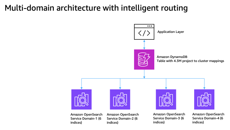
OpenSearch is an open source software suite for search, analytics, security monitoring, and observability applications, licensed under the Apache License V2.0. Amazon OpenSearch Service is a managed service that lets you deploy, scale, and operate OpenSearch and the Elasticsearch engine in the AWS Cloud. Customers run search workloads on OpenSearch Service at a scale of billions of documents. When a single index holds millions to billions of documents, you need to plan the topology of the OpenSearch Service domain that holds the index. This post walks through how Autodesk re-architected a single-index Elasticsearch 7.1.1 domain on Amazon OpenSearch Service into four multi-index OpenSearch Service domains, using Migration Assistant for Amazon OpenSearch Service and a routing layer that directs each query to the shards that hold the data for that query.

Autodesk is a technology company that serves customers across three industry verticals: Architecture, Engineering, and Construction (AEC), Product Design and Manufacturing, and Media and Entertainment. Autodesk’s mission is to empower everyone, everywhere to design and make anything, helping customers work across the boundaries of project, discipline, and industry.

Autodesk Forma (formerly Autodesk Construction Cloud, or ACC) is a cloud-based construction management and collaboration system. Customers across the globe use Autodesk Forma for workflows that include document management, bid management, quantification, coordination, design collaboration, project management and field collaboration. Autodesk Forma uses Amazon OpenSearch Service to provide a search experience for millions of users. As customers add data, the data that Forma stores in OpenSearch Service grows. In an OpenSearch Service domain, an index is the unit of data storage and organization. When an index reaches 100 TB, the index becomes a performance bottleneck and is hard to scale. As Autodesk Forma grew, Forma data management (formerly Autodesk Docs) hit performance and scaling limits. This component supports access and search across the project catalog.

Where Autodesk started

Forma data management ran on a single Elasticsearch 7.1.1 domain on Amazon OpenSearch Service with one index. The domain held about 100 TB of data on over 100 data nodes with over 400 primary shards and a replication factor of 1. The average shard held 200 GB. Because of the scale and the production state of the domain, tuning techniques such as adding shards, adding indices, or rebalancing data were not viable.

The single-index, single-domain design exposed three challenges to future data growth:

  1. Query performance. Query latency degraded over time as data grew.
  2. Vertical scaling. The team had reached the limit of the largest Amazon Elastic Compute Cloud (Amazon EC2) instance size available for the existing instance class.
  3. Horizontal scaling. Without a routing mechanism, adding nodes produced hot nodes inside the cluster managed by the OpenSearch Service domain.

Multi-domain architecture with intelligent routing

Vertical or horizontal scaling can address query performance in the short term, but neither addresses the underlying single-index, single-domain scalability limit. A horizontal scaling approach that uses routing keys gives you control over which shards each query touches, without requiring larger hardware. The Autodesk team applied this approach to re-architect the search service without impacting production traffic.

Four Amazon OpenSearch Service domains with an Amazon DynamoDB routing layer directing each query to the correct domain

Figure 1: Multi-domain architecture with intelligent routing

The architecture has the following properties:

  • Four Amazon OpenSearch Service domains on OpenSearch 2.19, each running 24 m7i.4xlarge.search nodes.
  • 24 indices total (6 per domain).
  • About 95 million documents per index.
  • 52 TB of primary storage. This is 37 percent smaller than the primary storage size of the original single-index domain, mainly because the migration skipped deleted documents.

The setup uses four horizontally scaled OpenSearch Service domains, with a routing layer that directs each query to the domain that holds the project’s data.

The architecture uses a Amazon DynamoDB table that stores 4.3 million routing records, one record per project. A project is the primary workspace in Forma data management, where teams, data, documents, models, workflows, permissions, issues, and collaboration activities live together. Forma application looks up the Amazon DynamoDB table for the project-to-domain mapping and then issues the search query to the correct domain.

Redistributing millions of records across four domains was hard. To find an even project-to-index allocation, the team used a bin-packing algorithm. A bin-packing algorithm packs items of varying sizes into a fixed number of bins to minimize waste and produce an even distribution. The team worked with 4.3 million projects of varying document counts, from a few documents per project up to millions, across 24 indices that each target around 400 million documents. The team implemented a stratified bin-packing algorithm that uses historical usage metrics for the workload. This algorithm avoids over- or under-allocation of resources during migration planning. To avoid over-allocation, the team used the 95th percentile (P95) usage metric. After applying the algorithm, each OpenSearch Service domain landed at about 49 percent utilization, which leaves a 2x growth buffer. The application then uses routing-key-based queries to search only the relevant shards, instead of every shard in the index.

The architecture has the following benefits:

  • Horizontal scalability. The team can add more domains and indices as needed.
  • Efficient routing. Queries hit specific shards, not every shard in the domain.
  • Reduced blast radius. If one domain becomes unavailable, only about 25% of traffic is affected, instead of full downtime under the single-domain design.
  • Independent scaling. The team can scale each domain based on its load pattern.
  • More search threads. The aggregate search-thread pool is larger across four domains than on one domain.

Migration steps

The following sections describe the four steps the Autodesk team followed to complete the migration.

Step 1: Categorize projects by size

The team grouped projects into four size categories by current document count, then collected data over six months to compute a per-category growth factor and extrapolate one year out:

Category Document range Project count % of total P95 growth factor Rationale
TINY 0 – 1,000 4,085,310 95.0% 3.82x Tiny projects grow fastest
SMALL 1,000 – 10,000 184,347 4.3% 2.11x Moderate growth expected
MEDIUM 10,000 – 100,000 28,385 0.66% 1.72x Slower relative growth
LARGE 100,000+ 2,266 0.05% 1.38x Already mature, minimal growth
Total 4,300,308 100%

The table shows that 95 percent of projects are TINY, but LARGE projects account for the bulk of document volume. The stratification by category lets the algorithm handle each category appropriately.

The Autodesk team analyzed document count per project over six months to estimate growth. Using the P95 growth factor per category gives a conservative capacity plan that covers 95 percent of projects and avoids over-provisioning.

Step 2: Interleaved distribution

If you process all LARGE projects first, you create imbalance across the indices. To avoid this imbalance, the bin-packing algorithm interleaves the categories in a round-robin pattern. The team used the following sequence to distribute documents evenly across the Amazon OpenSearch Service domains:

  1. Sort the projects within each category, largest first.
  2. Create a queue for each category. The queue is a first-in, first-out data structure that holds the sorted projects for one category.
  3. Distribute projects in a round-robin pattern: pick one from LARGE, then MEDIUM, then SMALL, then TINY, and repeat.

Step 3: Load-balanced best fit

After interleaving, the team computed the projected size of each project and assigned the project to an index. The following steps describe the approach:

  1. Compute the estimated future size as current size × growth factor.
  2. Use a priority queue to find the index with the most available capacity. In a priority queue, each element has a priority. Here, the priority of each index is the amount of available capacity the index has. Unlike a regular queue, a priority queue returns the highest-priority element first, not the first one inserted.
  3. Assign the project to the index that has the most available capacity.
  4. Update the index’s estimated load and re-insert the index into the priority queue with the new capacity. The re-insert step keeps the queue accurate for the next project assignment.

The preceding three steps produced the following results:

  • The algorithm distributed 4.3 million projects with 99.999 percent routing accuracy.
  • Project distribution across indices held to a 0.15 percent variance.
  • Each domain landed at 49.1 percent capacity utilization after applying growth factors, leaving 50.9 percent headroom for future growth.
  • The algorithm computed the 4.3 million project allocations in about 10 minutes.

The team stored the project-to-index allocation mapping in Amazon DynamoDB for real-time query routing. Routing controls how the application uses domain resources and how each domain performs. With routing, the application searches the shards that match the routing key (projectId) for that project. Without routing, the same query searches every shard in the index, which wastes domain resources and produces slower queries. The team also tuned the shard size, which matters most for large projects. One of the largest projects held 7 million documents at about 40 KB per document, for a total of about 280 GB. To split the data for that project into 20–25 GB shards, the team set routing_partition_size to 12.

Step 4: Migration with Migration Assistant for Amazon OpenSearch Service

The Autodesk team used the snapshot and re-index path in Migration Assistant for Amazon OpenSearch Service to migrate 2.3 billion documents. Migration Assistant for Amazon OpenSearch Service adapts to the migration profile and provides AWS Identity and Access Management (IAM) permission boundaries, Amazon Virtual Private Cloud (Amazon VPC) support, and the security policies the migration needs. Migration Assistant for Amazon OpenSearch Service integrated with the over 400 tasks that run the application on Amazon Elastic Container Service (Amazon ECS) with AWS Fargate.

Before the production cutover, the team ran several proof-of-concept (PoC) iterations and tuned the migration configuration to raise throughput from 18 GB/hr to 228 GB/hr. The first PoC iteration hit 18 GB/hr on m7g.large.search nodes. Each subsequent iteration added horizontal scale, larger instances (m7g.2xlarge.search and m7g.4xlarge.search), parallel writes across domains, and zero replicas during migration. The fourth and final PoC iteration hit 228 GB/hr. Multiple PoC iterations helped the team select the optimal instance size and instance class to migrate 2.3 billion documents in 6 hours with zero downtime and no customer incidents.

Post-migration analysis

After the team migrated 2.3 billion documents with routing enabled, the shards landed as follows:

Metric Result Target Status
Total primary shards 4,325
Total data size 52.11 TB ~52 TB ✓ On target
Average shard size 12.34 GB 10–15 GB ✓ Optimal
Median shard size 11.9 GB 10–15 GB ✓ Optimal
Shards in optimal range (10–15 GB) 75.5% 70% ✓ Above target
Hot shards (> 30 GB) 12 (0.28%) < 1% ✓ Within limit
Undersized shards (< 10 GB) 528 (12.2%) < 15% ✓ Within limit
Cross-domain balance 2.3% variance < 5% ✓ Within target
Node balance (StdDev) 0.78–1.12 shards < 2 ✓ Within target

The following table compares the pre- and post-migration architectures:

Aspect Old (single domain) New (four domains with intelligent routing)
Shard size 200 GB average 12.34 GB average (94% reduction)
Query broadcast All 400+ shards ~12 shards (97% reduction)
Shards in optimal range 0% 75.5%
Cross-domain balance N/A (single domain) 2.3% variance
Storage 83.3 TB 52 TB
Total P99 query latency 17 seconds 5 seconds

The team migrated 2.3 billion documents in about 6 hours. Storage dropped by about 37 percent, from 83.3 TB to 52 TB, because the migration dropped deleted documents. The migration produced 4,325 shards at an average of 12.34 GB per shard, distributed across the four domains. 75.5 percent of shards landed in the 10–15 GB range, compared to 210 GB before the migration, which confirms that the new architecture solves the large-shard problem. The shard size is as per general guidance where search latency is a key performance objective. Cross-domain variance of 2.3 percent (12.85 TB to 13.15 TB per domain) confirms even data distribution.

After the migration, queries that include the projectId routing key scan only the relevant shards (typically 12 of 180 per index), which reduces search load across shards by 93 percent. Routing also balances CPU and memory use across each domain. The routing_partition_size of 12 per index produced the right shard count per index. Overall P99 latency improved by 72 percent, from 17 seconds to 5 seconds. Within that figure, search-query P99 improved by 92 percent, from 2,500 ms to 200 ms.

Lessons learned

The PoC iterations surfaced several lessons. Larger instance types help query performance in the short term, but query routing combined with horizontal scaling produces higher sustained throughput. During bulk loads, disable replicas and increase the refresh interval to reduce write overhead. Plan for enough IP addresses and subnet capacity when you scale the application out, so that you do not hit a service limit mid-migration. Validate the VPC routing configuration between the application and the OpenSearch Service domains. Confirm OpenSearch Service data-node capacity with AWS Support before a horizontal scale-out. The Amazon DynamoDB-based routing layer adds about 20 ms of routing latency per query, but the routing layer cuts overall search latency and unlocks horizontal scale.

Conclusion

In this post, you saw how the Autodesk team migrated 2.3 billion documents from a single-index domain to four multi-index Amazon OpenSearch Service domains in about 6 hours.

Transitioning to a multi-domain architecture or updating to the latest OpenSearch version has historically been complex. It can also be difficult to predict the outcome of a migration before production traffic moves. The Migration Assistant for Amazon OpenSearch Service solution addresses these challenges by making migration workflow-driven, repeatable, and more straightforward to validate before cutover.

Migration Assistant for Amazon OpenSearch Service coupled with Amazon DynamoDB-based intelligent routing helped achieve balanced shards and improved search query performance. Multiple PoC iterations helped find routing bugs, service-quota limitations, and infrastructure-provisioning gaps before the production cutover.

If you plan to migrate a large dataset between OpenSearch Service domains, you can use Migration Assistant for Amazon OpenSearch Service. For more information, see the Migration Assistant for Amazon OpenSearch Service documentation.


About the authors

Ambarish Rao

Ambarish Rao

Ambarish is a Principal Engineer at Autodesk Search Team. He is based out of Pune. With 11 years of experience across financial data, logistics and now design and manufacturing, he has worked on mid to large scale distributed systems. When not working on Search, he’s either swimming, playing badminton, volunteering to teach kids, or hunting for Pune’s best biryani.

Chengsi Xie

Chengsi Xie

Chengsi is a Software Development Engineer on Autodesk Search Team. He is focused on building scalable distributed search platforms. He enjoys digging into the root causes behind problems and understanding how systems behave. Outside of work, he likes to stay active through running, playing badminton, hiking, and other outdoor activities that help him stay energized and grounded.

Manoj Kale

Manoj Kale

Manoj is a Senior Solutions Architect at Amazon Web Services. He helps customers design and build scalable, resilient solutions on AWS. He specializes in cloud architecture, AI/ML, and DevOps, and enjoys working with customers to solve complex technical challenges. Outside of work, he likes to spend time with family, travel and log the travel through travel logs and photos.

Anirudh Gupta

Anirudh Gupta

Anirudh is a Technical Account Manager at Amazon Web Services. He works closely with enterprise customers to help them architect, optimize, and operate their workloads on AWS. He is passionate about helping customers modernize their infrastructure and scale distributed systems on AWS.

Priyanshi Omer

Priyanshi Omer

Priyanshi is a Solutions Architect at Amazon Web Services. She helps customers design and build scalable, resilient solutions on AWS. She specializes in cloud architecture, AI/ML, and DevOps, and enjoys working with customers to solve complex technical challenges.

Trace cascading decision failures with a blame graph on Amazon OpenSearch Service

Post Syndicated from Jon Handler original https://aws.amazon.com/blogs/big-data/trace-cascading-decision-failures-with-a-blame-graph-on-amazon-opensearch-service/

Multi-agent systems are straightforward to build but hard to debug. You chain a few agents together, each one does its part, and most of the time it works. When it doesn’t, you’re left with a large volume of logs. They tell you what every agent said, but nothing about which agent caused the bad outcome.

Working with AWS customers building multi-agent systems, we kept seeing the same problem. A pipeline of agents decides, the decision turns out wrong, and no one can say which agent caused it. The logs are complete, but they don’t answer that question. So we, two AWS Solutions Architects, built a stock-research pipeline to reproduce it and show a solution approach.

Five agents work in sequence, and the last one makes a BUY, SELL, or HOLD call. In our test cases, the agent kept recommending BUY, and the positions kept losing money. Every step was logged. The logs still didn’t tell us who broke the pipeline.

In this post, we show you how to build a blame graph that traces which agent caused a failure in a multi-agent pipeline, using Amazon OpenSearch Service for graph storage and Amazon Bedrock for embeddings and reasoning.

Prerequisites

You must have the following prerequisites to follow along with this post.

  • Download the source code from the GitHub repository: It includes everything needed to set up and run the demo end to end:
    • The five-agent pipeline.
    • The instrumentation layer.
    • AWS CloudFormation template.
    • OpenSearch UI dashboard export
    • Sample data.
    • Step-by-step setup instructions (README.md, DEPLOYMENT.md).
  • An AWS account with access to Amazon Bedrock (Anthropic Claude Sonnet 4.5 and Amazon Titan Text Embeddings V2 enabled in us-west-2).
  • An OpenSearch Service domain.
  • Python 3.11+.
  • AWS Command Line Interface (AWS CLI) v2 configured with valid credentials.

The challenge

The pipeline is a chain of five agents. A Researcher gathers the facts, a Risk Analyst weighs the downside, a Valuation Analyst runs the numbers, and a Macro Economist sets up the market backdrop. Each one builds on the output of the agents before it. The Strategist (AI agent) sits at the end and turns all of it into a single call: BUY, SELL, or HOLD.

We set up three failures, each one a pattern common in production agent deployments (hallucinated facts from retrieval, suppressed minority signals, stale data from delayed ingestion):

  • A hallucination. The Researcher invents a company partnership that doesn’t exist.
  • A buried warning. The Risk Analyst flags a regulatory risk and gets outvoted.
  • Stale data. The Researcher misses a filing published three days earlier.

We engineered each failure deterministically, so the demo is reproducible and has a known answer. For each scenario, we hand-authored the five agents’ outputs as fixed JavaScript Object Notation (JSON). The pipeline replays these outputs while the instrumentation computes embeddings, influence, and blame live. We recorded a ground-truth root cause (for example, researcher for hallucination).

In every case, the pipeline recommends BUY, and the position drops. Standard logging records each agent’s output, but it can’t tell you which claim drove the final decision. Closing the gap between logging and root-cause attribution is what we set out to do.

Solution

We treat agent reasoning as a graph and measure influence between agents, then walk that graph backward from the failed decision to find the root cause.

Three services make up the stack:

  • Strands Agents runs the five-agent pipeline.
  • Amazon Bedrock provides the models: Amazon Titan Text Embeddings V2 to embed each claim, and Anthropic Claude Sonnet 4.5 for agent reasoning and the incident write-up.
  • AOpenSearch UI applicationan analytics interface hosted in the AWS Cloud with a single endpoint, connects to the domain as a data source and serves the dashboard, Discover, and the Dev Tools console we use to investigate. 

Here is how blame attribution works. Every claim an agent makes becomes a document with an Amazon Titan embedding. When a downstream agent cites something, we measure the cosine similarity between that citation and each upstream claim. Cosine similarity becomes the influence one agent had on another.

We store these as edges. To find the root cause, we start at the failed decision and walk backward through the edges. Whoever contributed the most gets the most blame.

Alongside the graph we record three things per run: an explainability score for how much of the decision traces back to evidence, the confidence of the attribution, and whether a dissenting agent was overruled.

A note on method: there is no industry standard yet for root-cause attribution in multi-agent large language model (LLM) pipelines. Our approach combines two established ideas: a credit assignment (attributing an outcome to the steps that produced it) and embedding similarity for tracing how claims propagate, with an LLM-as-a-judge style check. The metrics here (influence, explainability) are pragmatic, reproducible measures we define in this post, not standardized benchmarks.

Architecture

Five parts make up the flow:

  • Agents run on the Strands Agents, with reasoning on Claude Sonnet 4.5.
  • An instrumentation layer extracts each claim, embeds it with Amazon Titan Text Embeddings V2, scores influence with cosine similarity, runs the backward traversal, and generates an incident report.
  • Amazon OpenSearch Service holds seven indices, including the claims index with k-nearest neighbor (kNN) vectors and the blame, metrics, and incident indices.
  • Analysts review the results in the OpenSearch UI application (the dashboard, Discover, and the Dev Tools console), launched from the Amazon OpenSearch Service console.
  • We use OpenSearch UI rather than the domain’s built-in dashboards. Because OpenSearch UI is hosted in the AWS Cloud, the application stays available during domain maintenance and can bring multiple data sources into one view. The pipeline still writes to the domain, and OpenSearch UI reads it as a registered data source. 
Five-agent pipeline: Researcher, Risk Analyst, Valuation, Macro Economist, Strategist in sequence, ending at BUY decision.

Figure 1a: The five-agent runtime pipeline

Instrumentation layer sending embeddings and blame edges to Amazon OpenSearch Service, with Amazon Bedrock providing Amazon Titan and Claude models.

Figure 1b: The instrumentation and OpenSearch Service data plane

Walking through a failure

We ran the pipeline nine times, three runs per scenario, on an Amazon OpenSearch Service domain running OpenSearch 2.17. The decision under investigation is the final BUY. We know it failed because each scenario carries a ground-truth outcome: the position lost money. The failure is the known bad outcome we trace backward from, not something the system infers.  Everything the pipeline produces is a document you can query, so the investigation is a series of queries we run from the Dev Tools console in the OpenSearch UI application. 

To follow along, launch the OpenSearch UI application from the Amazon OpenSearch Service console, open your workspace, and choose Dev Tools (near the bottom of the left navigation panel). Paste each query below into the left pane and choose the run button. Every query in this section is in the repository at devtools_queries.md, in the same order as the walkthrough, so you can copy them from there instead of retyping. The equivalent queries as Python are in queries.py. 

Start with the outcome

Every run is a BUY, and every loss is negative, down to 72 percent. Standard logging stops here. You know it failed, but you don’t know who to fix.

Dev Tools query results showing nine pipeline runs, all recommending BUY with losses from 58% to 72%.

Figure 2: Pipeline run results: all nine runs recommend BUY with losses up to 72%

Next, look at who influenced whom

Among all agents, the Researcher sources the most edges. Nearly every node downstream gets its data from the Researcher, making it the first place to look. A lead, not a verdict.

Dev Tools aggregation showing influence edges by source agent; Researcher has the most edges.

Figure 3: Influence edges aggregated by source agent

Query the blame metrics for each scenario

Blame lands on the Researcher, with a score around 0.45, and the attribution is correct on all three runs. A fabricated partnership flowed straight into the final BUY. Stale-data scenario behaves the same way: the Researcher again, at 0.46, correct.

Dev Tools query showing root cause attribution: Researcher at 0.45 for hallucination scenario.

Figure 4: Root cause attribution for hallucination runs

Here are the raw edges in Discover, sorted from highest influence to lowest

In the OpenSearch UI application, choose Discover and select the agent-blame index pattern, then set the time range to Last 30 days and sort by influence_score descending. Each row is one edge- a claim passed from a source agent (source_agent.agent_id) to a downstream agent (target_agent.agent_id), scored by how strongly it shaped that agent’s output. The top rows are the highest-influence edges: the ones that most shaped the final BUY.

Discover view of blame edges sorted by influence score, highest to lowest.

Figure 5: Blame edges sorted by influence score

When attribution is hard

It’s the buried-warning scenario that the graph gets wrong, and it’s the most useful result in the post.

The Risk Analyst was right. It flagged the regulatory risk. The Strategist saw the warning, weighted it at 0.15, and bought it anyway. Who actually failed? The Strategist.

But the blame graph points at the Risk Analyst, with the highest score in that run at 0.37. Why? Our method measures influence, and the dissent is a distinct claim that the method traces directly, so it scores high. Influence is not the same as responsibility.

Why did the Strategist ignore it? In the scenario, the Strategist acknowledged the dissent but reasoned that the strength of the clinical data made the compound “differentiated” from past failures. It weighted that bullish evidence at 0.85 against the Risk Analyst’s 0.15. The Strategist rationalized the warning away instead of treating high-confidence, time-bound regulatory risk as a hard stop. The model recorded that reasoning, which is exactly why we can see how the dissent was discounted.

This gap between influence and responsibility is why we track dissent on our own.

Dissent was present, acknowledged, and weighted at 0.15. A flag catches what the graph misses: a valid warning was heard and then ignored. One signal is not enough. Influence tells you what is propagated. Dissent flags tell you what was wrongly dismissed. You need both.

Dev Tools query showing suppressed dissent: dissent_weight_given 0.15, dissent_suppressed true.

Figure 6: Suppressed dissent detection

Reviewing the metrics dashboard

OpenSearch UI rolls up all nine runs. To open it, launch the OpenSearch UI application, open your workspace, and choose Dashboards in the left navigation, then open the Multi-Agent Blame Game — Observability dashboard. Set the time range to Last 30 days to see all nine runs. If you haven’t imported it yet, go to Manage Workspace and choose Import under Assets. Upload blame-game-dashboard.ndjson from the repository, mapping the index patterns to your domain’s data source.

Full OpenSearch metrics dashboard with panels for root cause, explainability, loss, influence, and propagation.

Figure 7: Full metrics dashboard

Each panel earns its place. A few are worth calling out. Root cause distribution flags the Researcher six times and the Risk Analyst three times. That Risk Analyst slice is the dissent misattribution from earlier, not a real culprit.

Root cause distribution: Researcher in 6 runs, Risk Analyst in 3 (misattribution).

Figure 8: Root cause distribution

Explainability averages 0.826, a metric we define, not a standard score.

Explainability score averaging 0.826 across nine runs.

Figure 9: Explainability score

Preventable loss versus realized loss splits the damage attribution can pin on one agent from the damage it can’t. And average influence clusters rather than spikes, showing no single cause. That is the whole reason attribution sums influence instead of trusting one edge.

Preventable loss panel showing dollar amounts attributed to root-cause agent per scenario.

Figure 10: Preventable loss

Realized loss panel showing total financial damage across all runs before attribution.

Figure 11: Realized loss

Blame and loss comparison table: hallucination and stale-data rows show small errors. Dissent row shows largest gap.

Figure 12: Blame and loss table

Average influence by source agent: scores cluster between 0.29 and 0.42, no single spike.

Figure 13: Average influence by source agent

Propagation type breakdown: most edges weak or independent, few amplified.

Figure 14: Propagation type breakdown

Exploring it interactively

For demos we wrapped the same pipeline in a small Streamlit app. To run it, from the repository root install the dependencies and start the app:   

source .env 
streamlit run src/app.py --server.address localhost

It opens in your browser at http://localhost:8501. It runs two ways: pick a prepared scenario and replay it, or type in a company of your own and have the five agents run live on Amazon Bedrock against it. Either way you watch the agents execute, and the blame graph form, with the verdict and the incident narrative on one screen. A History tab reads the metrics index, so you can review past runs without leaving the app. 

A live run has no ground truth, so the app doesn’t claim the attribution is right or wrong. You just see where the influence landed. The prepared scenarios are still the way to demonstrate a specific, known failure. 

Streamlit demo app showing a pipeline run with agent panels, claims, and blame verdict.

Figure 15: Streamlit demo app

Explaining every decision: The evidence each agent weighed

Blame attribution is only useful if you can see the evidence behind it. Every claim an agent makes is stored with the confidence the agent assigned and the source it came from. Sources include an SEC filing, a clinical trial registry, an FDA page, or an earnings call. A blame score is never a bare number. You can open any agent and read the exact claims and sources it weighed before it spoke.

Consider the final decision as the clearest example. The Strategist doesn’t only emit a BUY. The Strategist records which upstream claim it relied on and how much weight it gave each one. Recording those weights turns the last step from a black box into a list of citations you can audit.

Explainability captures exactly that. A high score means most of the recommendation traces back to specific, sourced claims rather than to unexplained reasoning. It is the difference between the model said BUY and the model said BUY because of these claims, from these sources, weighted this way.

Streamlit app detail: Financial Researcher claims expanded with confidence scores and sources.

Figure 16: Per-agent evidence and reasoning for the BioGenX run

Performance and results

Across nine runs, the system identified the correct root cause six times, or 67 percent. The three misses are all the buried-warning scenarios, where influence and responsibility diverge. We would rather report the real number and explain the miss than round it up.

A full run takes about 25 seconds from end to end. Almost all of that is the Bedrock calls: about 74 embeddings per run plus one Claude write-up.

Attribution alone, the part that walks the graph and assigns blame, runs in about 74 milliseconds. That is cheap enough to run on every pipeline execution, not only after something goes wrong.

End-to-end latency chart: full run about 25 seconds, attribution step about 74 milliseconds.

Figure 17: End-to-end latency scenario

What this means for building agent pipelines

Our data points at three concrete changes:

  • Make the Researcher cross-check any major claim against a second source.
  • Give the Strategist a hard rule so a high-confidence dissent near a binary event can’t be overridden silently.
  • Add a freshness check so old data can’t drive a decision.

More broadly, treat influence and responsibility as separate questions. Measure both. A blame graph is a strong default for tracing propagation, but you need side signals like dissent suppression to catch up on the cases it can’t see.

From detection to prevention: Guardrails that stop the loss

Attribution tells you who broke a run after the fact. The same signals can stop the break before anyone acts on it. We added a guardrail layer that sits between the pipeline’s decision and the action, and overrides the call when a known failure pattern appears. The demo implements this layer (run with --guardrails, or toggle it in the app). It answers the question of whether the fixes are in the code: they are.

Guardrail gate diagram: blame signals feed three checks (dissent-override, source cross-check, freshness) before decision passes or is held.

Figure 18: The guardrail gate between the decision and the action

Each guardrail targets one of the three failure modes:

  • Dissent-override (Strategist): When the Risk Analyst raises a high-confidence dissent near a binary event and the Strategist under-weights it, the decision is forced to the safe action (HOLD).
  • Source cross-check (Researcher): A material claim resting on a single self-reported source cannot drive a BUY. It must be corroborated, or the call is held.
  • Freshness (Researcher): If material information was published just before the analysis and was not reflected in the inputs, the call is held.

With all three enabled, every scenario that previously issued a losing BUY is caught and held. Across the three runs that is about USD $3.79 million of illustrative loss prevented.

Guardrails effect: approximately $3.79M illustrative loss converted from realized to prevented.

Figure 19: Guardrails convert realized loss into prevented loss

The three guardrails are demo-grade heuristics, and we want to be explicit about that. The single-source and freshness checks work here only because the scenario data is engineered with known sources and dates. They are proxies, not real controls. A well-formed hallucination with a plausible citation would pass without detection of the cross-check, and the freshness rule only knows about data it is handed.

To make this production-grade, replace each proxy with real control.

For hallucinations, don’t count sources. Verify the material claims a decision rests on against a trusted source such as a knowledge base in Amazon OpenSearch Service or an authoritative filings and market-data API. Use an entailment or LLM-as-a-judge check to confirm the evidence actually supports the claim, requiring corroboration from independent sources before a claim can drive a BUY.

For freshness, wire in a live data feed and a scheduled-catalyst calendar. Hold whenever a decision rests on inputs that predate a material update or sits too close to a binary event. For dissent, keep the override but calibrate its threshold on historical outcomes and route borderline, high-value calls to a human rather than auto-deciding.

Underneath all of it, store the rules and thresholds as versioned policy in OpenSearch Service. Keep the blame graph running so you can confirm the guardrails fire for the right reasons. Log every override for audit, and evaluate the whole layer on real outcomes. Watch the false-positive rate as closely as the catches, because a guardrail that blocks good trades is only a new failure mode. Stay conservative: Prefer holding a good trade to taking a bad one, and make every block explainable.

Responsible AI considerations

This solution uses Amazon Titan Text Embeddings V2 and Anthropic Claude Sonnet 4.5 for agent reasoning and incident narrative generation. LLM-generated blame attributions and incident reports are informational aids, not authoritative verdicts. Always pair automated attribution with human review before making operational decisions. The influence score measures semantic similarity between claims, not true causation. The buried-warning scenario in this post demonstrates exactly where that distinction matters.

All company names, financial figures, and scenarios are fictional. No real market data or customer information is used. The stock-research pipeline is an illustrative vehicle for demonstrating blame attribution and observability. It isn’t investment advice, and the BUY/SELL/HOLD outputs are not stock recommendations. Don’t use this system, as built, to make financial or investment decisions.

Before adapting this approach to production pipelines, validate attribution accuracy against your own ground-truth data and implement safeguards appropriate to your risk level. The guardrails module in this repo is a starting point, not a complete solution. For more information, see Responsible AI with AWS.

Clean up

To avoid ongoing charges, delete the Amazon OpenSearch Service domain when you are done. The demo uses a single CloudFormation stack, so one command removes everything.

aws cloudformation delete-stack --region us-west-2 --stack-name blame-game-demo

Amazon Bedrock is billed per request, so there is nothing to tear down there.

Conclusion

Multi-agent pipelines fail in ways logs can’t explain. By embedding each claim with Amazon Titan Text Embeddings V2, scoring influence in Amazon OpenSearch Service, and walking the graph backward from the failed decision, we turned “something broke” into “here is the agent that broke it, and here is the evidence.” We also showed where that approach falls short, and the extra signal that covers it.

Code, queries, and deployment steps are in the repository. The hard part isn’t the infrastructure. It’s deciding to measure influence and responsibility as two different things.

Learn more

To dive deeper, get the full source in the GitHub repository, and see the Amazon OpenSearch Service and Amazon Bedrock documentation to adapt this to your own pipelines.


About the authors

Jon Handler

Jon Handler

Jon is a Senior Principal Solutions Architect for Search Services at Amazon Web Services. Jon works closely with OpenSearch and Amazon OpenSearch Service, providing help and guidance to a broad range of customers who have search and log analytics workloads. Prior to joining AWS, Jon’s career ranged across distributed systems and search at startups and large organizations. His career as a software developer included four years of coding a large-scale, eCommerce search engine.

Smita Singh

Smita Singh

Smita is a Senior Solutions Architect at AWS. She comes with 20 years of experience in the industry. She focuses on defining technical strategic vision and works on architecture, design, and implementation of modern, scalable platforms for large-scale global enterprises and SaaS providers. She specializes in architecture and implementation of large-scale platform solutions for global enterprises and SaaS providers, with a focus on data, analytics, and generative AI workloads.

Python packaging council candidates announced

Post Syndicated from jzb original https://lwn.net/Articles/1088920/

The Python Software Foundation (PSF) has announced
the candidates
running for the Python packaging council that was approved by the Python steering council
in April
.

This inaugural election fills all five seats on the PPC. The two candidates
receiving the highest number of votes shall be designated Cohort A with a two
year term, and the three candidates receiving the next highest number of votes
shall be designated Cohort B with a one year term.

In future elections, each cohort will be elected for a full two-year term in
alternating years, so that roughly half of the PPC turns over each cycle.

There are 17 candidates running for the five open seats. PSF voting-eligible
members must affirm
their intention to vote
in this election by August 25. Voting begins on
September 1, and ends on September 15.

The collective thoughts of the interwebz