Post Syndicated from Matt Granger original https://www.youtube.com/watch?v=6OjHkK23Uqk
Moon
Post Syndicated from xkcd.com original https://xkcd.com/2809/

Kernel prepatch 6.5-rc4
Post Syndicated from corbet original https://lwn.net/Articles/939685/
The 6.5-rc4 kernel prepatch is out for
testing.
So here we are, and the 6.5 release cycle continues to look
entirely normal.In fact, it’s *so* normal that we have hit on a very particular
(and peculiar) pattern with the rc4 releases: we have had *exactly*
328 non-merge commits in rc4 in 6.2, 6.3 and now 6.5. Weird
coincidence.And honestly, that weird numerological coincidence is just about
the most interesting thing here.
DIY Garage Golf Simulator Without Sacrificing Parking!? 5 Minute Setup.
Post Syndicated from The Hook Up original https://www.youtube.com/watch?v=YLTVi-KWhFE
Nikon FTZIII with AF Motor – Come on Nikon!!
Post Syndicated from Matt Granger original https://www.youtube.com/watch?v=OFe7d06mhEM
Intel LGA4677 112L E1A and 64L E1B Brackets for Intel Xeon W-3400 and W-2400 Series
Post Syndicated from Eric Smith original https://www.servethehome.com/intel-lga4677-112l-e1a-and-64l-e1b-brackets-for-intel-xeon-w-3400-and-w-2400-series-asus/
In this article, we show how to tie the the Intel LGA4677 112L E1A and 64L E1B brackets to the correct Intel Xeon W-3400 and W-2400 CPUs
The post Intel LGA4677 112L E1A and 64L E1B Brackets for Intel Xeon W-3400 and W-2400 Series appeared first on ServeTheHome.
Comic for 2023.07.30 – Beating
Post Syndicated from Explosm.net original https://explosm.net/comics/beating-2
New Cyanide and Happiness Comic
wysb
Post Syndicated from Oglaf! -- Comics. Often dirty. original https://www.oglaf.com/wysb/


Fanless Intel N200 Firewall and Virtualization Appliance Review
Post Syndicated from Patrick Kennedy original https://www.servethehome.com/fanless-intel-n200-firewall-and-virtualization-appliance-review/
We take a look at the fanless Intel N200 firewall and virtualization appliance to see how this quad 2.5GbE unit stacks up to the N100 option
The post Fanless Intel N200 Firewall and Virtualization Appliance Review appeared first on ServeTheHome.
8-Track ‘Boombox’ repairs – Old & Older
Post Syndicated from Techmoan original https://www.youtube.com/watch?v=_hpLKp4Aaag
Седмицата (24–29 юли)
Post Syndicated from Надежда Радулова original https://www.toest.bg/sedmitsata-24-29-yuli/
Не съм очаквал, че в страната, в която съм израснал […] ще се наложи да се усещам несигурен,
гласи Facebook пост на актьора Самуел Финци от 22 юли. Ето какво пише и Еми Барух два дни по-късно:
Съпротивителните сили на нацията не никнат върху плоскостта на безпаметството. За тях трябва да се грижат – институции, лидери, интелектуалци. Писатели, артисти, чувствителни хора. А наоколо? Наоколо сте вие […] Защо мълчите, драги „демократи“, уважаеми „правилни хора“?
Написаното от Еми Барух и Самуел Финци не е без повод. Все по-честите прояви на антисемитизъм в България, чийто връх беше разпространеният колаж с изобразени хора в нацистки униформи, дърпащи човек с образа на Соломон Паси в затворнически дрехи, е тревожен знак, че в смърдящия ни политически котел започва да къкри особено токсична, лесно възпламенима смес. Такава, която застрашава да разгради и обезчовечи и без това увредената социална тъкан.
Затова прощавайте, драги приятели, уважаеми читатели! Прощавайте, че ви развалям юлското настроение с това горчиво начало на предваканционния бюлетин на „Тоест“. Истината е, че исках да го посветя на лятото и да ви препоръчам августовските фестивали в Пловдив и Банско, в Ковачевица и Созопол… Но уви, днес ми се струва по-важно да ви разкажа една друга история, случила се (не чак толкова) отдавна. История, която не повдига настроението, но посвоему повдига духа. Укрепва съпротивителните сили, за които говори Еми Барух.
През март 1943 г., по време на депортацията на евреите от Беломорска Тракия, Вардарска Македония и Пирот, депортация, за която българската държава носи пряка отговорност, Надежда Василева, 52-годишна медицинска сестра с прогимназиално образование,
единствена се осмелява да премине през полицейския кордон и да занесе вода на хората, дни наред затворени във вагоните на Ломската гара.
В следващите часове тя организира иначе пасивните си съграждани да осигуряват и носят храна, лекарства, свещи, кибрит, пелени и с помощта на няколко циганчета върви от вагон във вагон и ги раздава.* Това е може би последната храна и вода, последният знак на съпричастност към тези хора по пътя им към лагера на смъртта Треблинка, в който само за 15 месеца през 1942 и 1943 г. са унищожени между 700 000 и 900 000 души.
Но Надежда Василева е била самарянка, ще кажете, самата тя – майка и баба, имала е дълг да помага и да се грижи за уязвимите, за хората в нужда и беда, за болните, за децата, за пеленачетата. Естествено е било да се противопостави на този чудовищен акт. Как обаче тогава обясняваме нейната „единственост“?
Защо само тя? Защо само тя в цял Лом???
Да действаш „не-правилно“, против правилата, както действа Василева, е решение, преди всичко плод не на принадлежност към дадена група (на жените, на майките, на медицинските сестри, на жителите на Лом, на българите и пр.), а на морална рефлексия и на еманципирана индивидуална съвест, независима от наложените в дадения момент обществени правила.
Надежда Василева мисли и действа не като член на общност или общество, а като зрял морален субект –
тъкмо от позицията на своята непринадлежност, на своята „неправилност“, на своята, ако щете, историческа „самота“.
„Когато всички са виновни, никой не носи вина“, твърди Хана Аренд. И продължава по-нататък:
Не съществува такова нещо като колективна вина или колективна невинност; вината и невинността имат смисъл само когато са отнесени към отделно взети личности.
В действията на медицинската сестра от Лом наблюдаваме противопоставяне на индивидуално срещу колективно – и разбира се, пълна готовност да се поеме отговорността за това. В една човешка среда, подложена на извънмерно изпитание, зловещо изпразнена от определящите я ценности, Надежда Василева успява да постигне немислимото. Оттласква се от колективното в жест на несъгласие и проявява своята индивидуалност – единственият начин да остане на страната на човешкото, да докаже (включително на самата себе си) собствената си човешкост, а впоследствие да се опита да привлече и останалите на своя страна. Единствената възможна според нея страна.
Страната, която би трябвало да е единствено възможна за всички нас.
Надежда Василева не спасява ничий живот, но спасява идеята за човешкото. Именно това спасение е в ръцете ни всеки ден.
Жест, който дължим и на миналото, и на бъдещето, и на себе си тук, сега.
Затова и призивът ми в момент, в който проявите на антисемитизъм в България тревожно зачестяват и се усилват през определени политически и партийни „мегафони“ като тези на „Възраждане“, но не само, е следният:
Бъдете чувствителни, бъдете „неправилни“, бъдете еманципирани в мислите си, бъдете зрели морални субекти. Реагирайте.
Разговаряйте за случващото се с децата си, с родителите си, с приятелите си. Ако прецените, подпишете петицията, инициирана от Зорница Христова и подкрепена вече от над 500 души. Или пък напишете нещо от свое име, дайте му гласност. Надявам се, че все още е възможно да спрем атаката на расисткия токсин и да я преобърнем в смислен разговор за миналото. И за настоящето.
Нека да започнем този разговор още днес – с острия и навременен текст на Светла Енчева „Българската резистентност към антисемитизма“.
* * *
В последния ни брой преди ваканцията ви предлагаме да прочетете още:
➜ за безскрупулното поведение на мобилния оператор „А1 България“ – Йовко Ламбрев, „От А1 с любов“;
➜ за това как управляващите партньори приключват политическия сезон – Емилия Милчева, „Коалицията по(тегли). Жегата мина“;
➜ за популистките клишета в политиката – Александър Нуцов, „Националният суверенитет и националният популизъм“;
➜ за телата – човешки и небесни – Михаил Ангелов, „Научни новини: Механизми за предпазване от болести, проблеми във „Фукушима“ и поздрави от съзвездието Кентавър“;
➜ за децата майки и трудовия пазар – Мирела Петкова, „Ранната бременност или бедността – яйцето или кокошката?“;
➜ за две новоизлезли книги, занимаващи се със сложните отношения между паметта и истината – Зорница Христова, „По буквите – Расучану, Кенаров“;
➜ и стихотворението на месец юли от авторката на „Единайсетте сестри на юли“ – Албена Тодорова, „Ако ние сме риби, които плуват в морето“.
Накрая, преди да се разделим, ви пожелавам приятно четене в дни на спокойствие и смисъл! И за да не заспим задълго под безветрието на летните сенки, ето едно парче на Робърт Алън Цимерман, известен като Боб Дилън – A Hard Rain’s A-Gonna Fall („Страшен дъжд ще падне“), което да ни държи нащрек и да ни напомня защо сме тук.
* За действията си по време на депортацията, на 18 декември 2001 г. Надежда Василева е провъзгласена от израелската комисия към Израелския институт „Яд Вашем“ за „праведник на света“.
Comic for 2023.07.29 – Baby Shoes
Post Syndicated from Explosm.net original https://explosm.net/comics/baby-shoes-2
New Cyanide and Happiness Comic
No-GIL mode coming for Python
Post Syndicated from corbet original https://lwn.net/Articles/939568/
The Python Steering Council has announced
its intent to accept PEP
703 (Making the Global Interpreter Lock Optional in CPython), with
initial support possibly showing up in the 3.13 release. There are still
some details to work out, though.
We want to be very careful with backward compatibility. We do not
want another Python 3 situation, so any changes in third-party code
needed to accommodate no-GIL builds should just work in with-GIL
builds (although backward compatibility with older Python versions
will still need to be addressed). This is not Python 4. We are
still considering the requirements we want to place on ABI
compatibility and other details for the two builds and the effect
on backward compatibility.
Friday Squid Blogging: Zaqistan Flag
Post Syndicated from Bruce Schneier original https://www.schneier.com/blog/archives/2023/07/friday-squid-blogging-zaqistan-flag.html
The fictional nation of Zaqistan (in Utah) has a squid on its flag.
As usual, you can also use this squid post to talk about the security stories in the news that I haven’t covered.
Read my blog posting guidelines here.
Highlights: The Science Behind Mixology | Devin Kidner | Talks at Google
Post Syndicated from Talks at Google original https://www.youtube.com/watch?v=YjfqFKTA5qk
Exploiting the StackRot vulnerability
Post Syndicated from corbet original https://lwn.net/Articles/939542/
For those who are interested in the gory details of how the StackRot vulnerability works, Ruihan Li has
posted a detailed
writeup of the bug and how it can be exploited.
As StackRot is a Linux kernel vulnerability found in the memory
management subsystem, it affects almost all kernel configurations
and requires minimal capabilities to trigger. However, it should be
noted that maple nodes are freed using RCU callbacks, delaying the
actual memory deallocation until after the RCU grace
period. Consequently, exploiting this vulnerability is considered
challenging.To the best of my knowledge, there are currently no publicly
available exploits targeting use-after-free-by-RCU (UAFBR)
bugs. This marks the first instance where UAFBR bugs have been
proven to be exploitable, even without the presence of
CONFIG_PREEMPT or CONFIG_SLAB_MERGE_DEFAULT settings.
New – AWS Public IPv4 Address Charge + Public IP Insights
Post Syndicated from Jeff Barr original https://aws.amazon.com/blogs/aws/new-aws-public-ipv4-address-charge-public-ip-insights/
We are introducing a new charge for public IPv4 addresses. Effective February 1, 2024 there will be a charge of $0.005 per IP per hour for all public IPv4 addresses, whether attached to a service or not (there is already a charge for public IPv4 addresses you allocate in your account but don’t attach to an EC2 instance).
Public IPv4 Charge
As you may know, IPv4 addresses are an increasingly scarce resource and the cost to acquire a single public IPv4 address has risen more than 300% over the past 5 years. This change reflects our own costs and is also intended to encourage you to be a bit more frugal with your use of public IPv4 addresses and to think about accelerating your adoption of IPv6 as a modernization and conservation measure.
This change applies to all AWS services including Amazon Elastic Compute Cloud (Amazon EC2), Amazon Relational Database Service (RDS) database instances, Amazon Elastic Kubernetes Service (EKS) nodes, and other AWS services that can have a public IPv4 address allocated and attached, in all AWS regions (commercial, AWS China, and GovCloud). Here’s a summary in tabular form:
| Public IP Address Type | Current Price/Hour (USD) | New Price/Hour (USD) (Effective February 1, 2024) |
| In-use Public IPv4 address (including Amazon provided public IPv4 and Elastic IP) assigned to resources in your VPC, Amazon Global Accelerator, and AWS Site-to-site VPN tunnel | No charge | $0.005 |
| Additional (secondary) Elastic IP Address on a running EC2 instance | $0.005 | $0.005 |
| Idle Elastic IP Address in account | $0.005 | $0.005 |
The AWS Free Tier for EC2 will include 750 hours of public IPv4 address usage per month for the first 12 months, effective February 1, 2024. You will not be charged for IP addresses that you own and bring to AWS using Amazon BYOIP.
Starting today, your AWS Cost and Usage Reports automatically include public IPv4 address usage. When this price change goes in to effect next year you will also be able to use AWS Cost Explorer to see and better understand your usage.
As I noted earlier in this post, I would like to encourage you to consider accelerating your adoption of IPv6. A new blog post shows you how to use Elastic Load Balancers and NAT Gateways for ingress and egress traffic, while avoiding the use of a public IPv4 address for each instance that you launch. Here are some resources to show you how you can use IPv6 with widely used services such as EC2, Amazon Virtual Private Cloud (Amazon VPC), Amazon Elastic Kubernetes Service (EKS), Elastic Load Balancing, and Amazon Relational Database Service (RDS):
- Dual Stack and IPv6-only Amazon VPC Reference Architectures (pdf)
- Dual-stack IPv6 architectures for AWS and hybrid networks – Part 1
- Dual-stack IPv6 architectures for AWS and hybrid networks – Part 2
- IPv6 on AWS
- AWS Services that Support IPv6
Earlier this year we enhanced EC2 Instance Connect and gave it the ability to connect to your instances using private IPv4 addresses. As a result, you no longer need to use public IPv4 addresses for administrative purposes (generally using SSH or RDP).
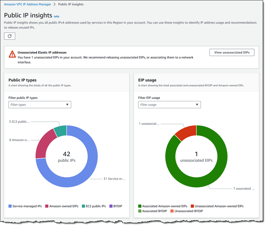
Public IP Insights
In order to make it easier for you to monitor, analyze, and audit your use of public IPv4 addresses, today we are launching Public IP Insights, a new feature of Amazon VPC IP Address Manager that is available to you at no cost. In addition to helping you to make efficient use of public IPv4 addresses, Public IP Insights will give you a better understanding of your security profile. You can see the breakdown of public IP types and EIP usage, with multiple filtering options:
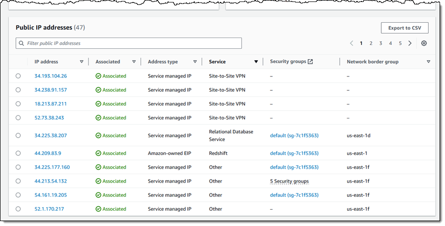
You can also see, sort, filter, and learn more about each of the public IPv4 addresses that you are using:
Using IPv4 Addresses Efficiently
By using the new IP Insights tool and following the guidance that I shared above, you should be ready to update your application to minimize the effect of the new charge. You may also want to consider using AWS Direct Connect to set up a dedicated network connection to AWS.
Finally, be sure to read our new blog post, Identify and Optimize Public IPv4 Address Usage on AWS, for more information on how to make the best use of public IPv4 addresses.
— Jeff;
A side-by-side comparison of Apache Spark and Apache Flink for common streaming use cases
Post Syndicated from Deepthi Mohan original https://aws.amazon.com/blogs/big-data/a-side-by-side-comparison-of-apache-spark-and-apache-flink-for-common-streaming-use-cases/
Apache Flink and Apache Spark are both open-source, distributed data processing frameworks used widely for big data processing and analytics. Spark is known for its ease of use, high-level APIs, and the ability to process large amounts of data. Flink shines in its ability to handle processing of data streams in real-time and low-latency stateful computations. Both support a variety of programming languages, scalable solutions for handling large amounts of data, and a wide range of connectors. Historically, Spark started out as a batch-first framework and Flink began as a streaming-first framework.
In this post, we share a comparative study of streaming patterns that are commonly used to build stream processing applications, how they can be solved using Spark (primarily Spark Structured Streaming) and Flink, and the minor variations in their approach. Examples cover code snippets in Python and SQL for both frameworks across three major themes: data preparation, data processing, and data enrichment. If you are a Spark user looking to solve your stream processing use cases using Flink, this post is for you. We do not intend to cover the choice of technology between Spark and Flink because it’s important to evaluate both frameworks for your specific workload and how the choice fits in your architecture; rather, this post highlights key differences for use cases that both these technologies are commonly considered for.
Apache Flink offers layered APIs that offer different levels of expressiveness and control and are designed to target different types of use cases. The three layers of API are Process Functions (also known as the Stateful Stream Processing API), DataStream, and Table and SQL. The Stateful Stream Processing API requires writing verbose code but offers the most control over time and state, which are core concepts in stateful stream processing. The DataStream API supports Java, Scala, and Python and offers primitives for many common stream processing operations, as well as a balance between code verbosity or expressiveness and control. The Table and SQL APIs are relational APIs that offer support for Java, Scala, Python, and SQL. They offer the highest abstraction and intuitive, SQL-like declarative control over data streams. Flink also allows seamless transition and switching across these APIs. To learn more about Flink’s layered APIs, refer to layered APIs.
Apache Spark Structured Streaming offers the Dataset and DataFrames APIs, which provide high-level declarative streaming APIs to represent static, bounded data as well as streaming, unbounded data. Operations are supported in Scala, Java, Python, and R. Spark has a rich function set and syntax with simple constructs for selection, aggregation, windowing, joins, and more. You can also use the Streaming Table API to read tables as streaming DataFrames as an extension to the DataFrames API. Although it’s hard to draw direct parallels between Flink and Spark across all stream processing constructs, at a very high level, we could say Spark Structured Streaming APIs are equivalent to Flink’s Table and SQL APIs. Spark Structured Streaming, however, does not yet (at the time of this writing) offer an equivalent to the lower-level APIs in Flink that offer granular control of time and state.
Both Flink and Spark Structured Streaming (referenced as Spark henceforth) are evolving projects. The following table provides a simple comparison of Flink and Spark capabilities for common streaming primitives (as of this writing).
| . | Flink | Spark |
| Row-based processing | Yes | Yes |
| User-defined functions | Yes | Yes |
| Fine-grained access to state | Yes, via DataStream and low-level APIs | No |
| Control when state eviction occurs | Yes, via DataStream and low-level APIs | No |
| Flexible data structures for state storage and querying | Yes, via DataStream and low-level APIs | No |
| Timers for processing and stateful operations | Yes, via low level APIs | No |
In the following sections, we cover the greatest common factors so that we can showcase how Spark users can relate to Flink and vice versa. To learn more about Flink’s low-level APIs, refer to Process Function. For the sake of simplicity, we cover the four use cases in this post using the Flink Table API. We use a combination of Python and SQL for an apples-to-apples comparison with Spark.
Data preparation
In this section, we compare data preparation methods for Spark and Flink.
Reading data
We first look at the simplest ways to read data from a data stream. The following sections assume the following schema for messages:
Reading data from a source in Spark Structured Streaming
In Spark Structured Streaming, we use a streaming DataFrame in Python that directly reads the data in JSON format:
Note that we have to supply a schema object that captures our stock ticker schema (stock_ticker_schema). Compare this to the approach for Flink in the next section.
Reading data from a source using Flink Table API
For Flink, we use the SQL DDL statement CREATE TABLE. You can specify the schema of the stream just like you would any SQL table. The WITH clause allows us to specify the connector to the data stream (Kafka in this case), the associated properties for the connector, and data format specifications. See the following code:
JSON flattening
JSON flattening is the process of converting a nested or hierarchical JSON object into a flat, single-level structure. This converts multiple levels of nesting into an object where all the keys and values are at the same level. Keys are combined using a delimiter such as a period (.) or underscore (_) to denote the original hierarchy. JSON flattening is useful when you need to work with a more simplified format. In both Spark and Flink, nested JSONs can be complicated to work with and may need additional processing or user-defined functions to manipulate. Flattened JSONs can simplify processing and improve performance due to reduced computational overhead, especially with operations like complex joins, aggregations, and windowing. In addition, flattened JSONs can help in easier debugging and troubleshooting data processing pipelines because there are fewer levels of nesting to navigate.
JSON flattening in Spark Structured Streaming
JSON flattening in Spark Structured Streaming requires you to use the select method and specify the schema that you need flattened. JSON flattening in Spark Structured Streaming involves specifying the nested field name that you’d like surfaced to the top-level list of fields. In the following example, company_info is a nested field and within company_info, there’s a field called company_name. With the following query, we’re flattening company_info.name to company_name:
JSON flattening in Flink
In Flink SQL, you can use the JSON_VALUE function. Note that you can use this function only in Flink versions equal to or greater than 1.14. See the following code:
The term lax in the preceding query has to do with JSON path expression handling in Flink SQL. For more information, refer to System (Built-in) Functions.
Data processing
Now that you have read the data, we can look at a few common data processing patterns.
Deduplication
Data deduplication in stream processing is crucial for maintaining data quality and ensuring consistency. It enhances efficiency by reducing the strain on the processing from duplicate data and helps with cost savings on storage and processing.
Spark Streaming deduplication query
The following code snippet is related to a Spark Streaming DataFrame named stock_ticker. The code performs an operation to drop duplicate rows based on the symbol column. The dropDuplicates method is used to eliminate duplicate rows in a DataFrame based on one or more columns.
Flink deduplication query
The following code shows the Flink SQL equivalent to deduplicate data based on the symbol column. The query retrieves the first row for each distinct value in the symbol column from the stock_ticker stream, based on the ascending order of proctime:
Windowing
Windowing in streaming data is a fundamental construct to process data within specifications. Windows commonly have time bounds, number of records, or other criteria. These time bounds bucketize continuous unbounded data streams into manageable chunks called windows for processing. Windows help in analyzing data and gaining insights in real time while maintaining processing efficiency. Analyses or operations are performed on constantly updating streaming data within a window.
There are two common time-based windows used both in Spark Streaming and Flink that we will detail in this post: tumbling and sliding windows. A tumbling window is a time-based window that is a fixed size and doesn’t have any overlapping intervals. A sliding window is a time-based window that is a fixed size and moves forward in fixed intervals that can be overlapping.
Spark Streaming tumbling window query
The following is a Spark Streaming tumbling window query with a window size of 10 minutes:
Flink Streaming tumbling window query
The following is an equivalent tumbling window query in Flink with a window size of 10 minutes:
Spark Streaming sliding window query
The following is a Spark Streaming sliding window query with a window size of 10 minutes and slide interval of 5 minutes:
Flink Streaming sliding window query
The following is a Flink sliding window query with a window size of 10 minutes and slide interval of 5 minutes:
Handling late data
Both Spark Structured Streaming and Flink support event time processing, where a field within the payload can be used for defining time windows as distinct from the wall clock time of the machines doing the processing. Both Flink and Spark use watermarking for this purpose.
Watermarking is used in stream processing engines to handle delays. A watermark is like a timer that sets how long the system can wait for late events. If an event arrives and is within the set time (watermark), the system will use it to update a request. If it’s later than the watermark, the system will ignore it.
In the preceding windowing queries, you specify the lateness threshold in Spark using the following code:
This means that any records that are 3 minutes late as tracked by the event time clock will be discarded.
In contrast, with the Flink Table API, you can specify an analogous lateness threshold directly in the DDL:
Note that Flink provides additional constructs for specifying lateness across its various APIs.
Data enrichment
In this section, we compare data enrichment methods with Spark and Flink.
Calling an external API
Calling external APIs from user-defined functions (UDFs) is similar in Spark and Flink. Note that your UDF will be called for every record processed, which can result in the API getting called at a very high request rate. In addition, in production scenarios, your UDF code often gets run in parallel across multiple nodes, further amplifying the request rate.
For the following code snippets, let’s assume that the external API call entails calling the function:
External API call in Spark UDF
The following code uses Spark:
External API call in Flink UDF
For Flink, assume we define the UDF callExternalAPIUDF, which takes as input the ticker symbol symbol and returns enriched information about the symbol via a REST endpoint. We can then register and call the UDF as follows:
Flink UDFs provide an initialization method that gets run one time (as opposed to one time per record processed).
Note that you should use UDFs judiciously as an improperly implemented UDF can cause your job to slow down, cause backpressure, and eventually stall your stream processing application. It’s advisable to use UDFs asynchronously to maintain high throughput, especially for I/O-bound use cases or when dealing with external resources like databases or REST APIs. To learn more about how you can use asynchronous I/O with Apache Flink, refer to Enrich your data stream asynchronously using Amazon Kinesis Data Analytics for Apache Flink.
Conclusion
Apache Flink and Apache Spark are both rapidly evolving projects and provide a fast and efficient way to process big data. This post focused on the top use cases we commonly encountered when customers wanted to see parallels between the two technologies for building real-time stream processing applications. We’ve included samples that were most frequently requested at the time of this writing. Let us know if you’d like more examples in the comments section.
About the author
 Deepthi Mohan is a Principal Product Manager on the Amazon Kinesis Data Analytics team.
 Karthi Thyagarajan was a Principal Solutions Architect on the Amazon Kinesis team.
Extend your data mesh with Amazon Athena and federated views
Post Syndicated from Saurabh Bhutyani original https://aws.amazon.com/blogs/big-data/extend-your-data-mesh-with-amazon-athena-and-federated-views/
Amazon Athena is a serverless, interactive analytics service built on the Trino, PrestoDB, and Apache Spark open-source frameworks. You can use Athena to run SQL queries on petabytes of data stored on Amazon Simple Storage Service (Amazon S3) in widely used formats such as Parquet and open-table formats like Apache Iceberg, Apache Hudi, and Delta Lake. However, Athena also allows you to query data stored in 30 different data sources—in addition to Amazon S3—including relational, non-relational, and object stores running on premises or in other cloud environments.
In Athena, we refer to queries on non-Amazon S3 data sources as federated queries. These queries run on the underlying database, which means you can analyze the data without learning a new query language and without the need for separate extract, transform, and load (ETL) scripts to extract, duplicate, and prepare data for analysis.
Recently, Athena added support for creating and querying views on federated data sources to bring greater flexibility and ease of use to use cases such as interactive analysis and business intelligence reporting. Athena also updated its data connectors with optimizations that improve performance and reduce cost when querying federated data sources. The updated connectors use dynamic filtering and an expanded set of predicate pushdown optimizations to perform more operations in the underlying data source rather than in Athena. As a result, you get faster queries with less data scanned, especially on tables with millions to billions of rows of data.
In this post, we show how to create and query views on federated data sources in a data mesh architecture featuring data producers and consumers.
The term data mesh refers to a data architecture with decentralized data ownership. A data mesh enables domain-oriented teams with the data they need, emphasizes self-service, and promotes the notion of purpose-built data products. In a data mesh, data producers expose datasets to the organization and data consumers subscribe to and consume the data products created by producers. By distributing data ownership to cross-functional teams, a data mesh can foster a culture of collaboration, invention, and agility around data.
Let’s dive into the solution.
Solution overview
For this post, imagine a hypothetical ecommerce company that uses multiple data sources, each playing a different role:
- In an S3 data lake, ecommerce records are stored in a table named
Lineitems - Amazon ElastiCache for Redis stores
NationsandActiveOrdersdata, ensuring ultra-fast reads of operational data by downstream ecommerce systems - On Amazon Relational Database Service (Amazon RDS), MySQL is used to store data like email addresses and shipping addresses in the Orders, Customer, and Suppliers tables
- For flexibility and low-latency reads and writes, an Amazon DynamoDB table holds
PartandPartsuppdata
We want to query these data sources in a data mesh design. In the following sections, we set up Athena data source connectors for MySQL, DynamoDB, and Redis, and then run queries that perform complex joins across these data sources. The following diagram depicts our data architecture.

As you proceed with this solution, note that you will create AWS resources in your account. We have provided you with an AWS CloudFormation template that defines and configures the required resources, including the sample MySQL database, S3 tables, Redis store, and DynamoDB table. The template also creates the AWS Glue database and tables, S3 bucket, Amazon S3 VPC endpoint, AWS Glue VPC endpoint, and other AWS Identity and Access Management (IAM) resources that are used in the solution.
The template is designed to demonstrate how to use federated views in Athena, and is not intended for production use without modification. Additionally, the template uses the us-east-1 Region and will not work in other Regions without modification. The template creates resources that incur costs while they are in use. Follow the cleanup steps at the end of this post to delete the resources and avoid unnecessary charges.
Prerequisites
Before you launch the CloudFormation stack, ensure you have the following prerequisites:
- An AWS account that provides access to AWS services
- An IAM user with an access key and secret key to configure the AWS Command Line Interface (AWS CLI), and permissions to create an IAM role, IAM policies, and stacks in AWS CloudFormation
Create resources with AWS CloudFormation
To get started, complete the following steps:
- Choose Launch Stack:

- Select I acknowledge that this template may create IAM resources.
The CloudFormation stack takes approximately 20–30 minutes to complete. You can monitor its progress on the AWS CloudFormation console. When status reads CREATE_COMPLETE, your AWS account will have the resources necessary to implement this solution.
Deploy connectors and connect to data sources
With our resources provisioned, we can begin to connect the dots in our data mesh. Let’s start by connecting the data sources created by the CloudFormation stack with Athena.
- On the Athena console, choose Data sources in the navigation pane.
- Choose Create data source.
- For Data sources, select MySQL, then choose Next.
- For Data source name, enter a name, such as
mysql. The Athena connector for MySQL is an AWS Lambda function that was created for you by the CloudFormation template. - For Connection details, choose Select or enter a Lambda function.
- Choose
mysql, then choose Next. - Review the information and choose Create data source.
- Return to the Data sources page and choose
mysql. - On the connector details page, choose the link under Lambda function to access the Lambda console and inspect the function associated with this connector.

- Return to the Athena query editor.
- For Data source, choose
mysql. - For Database, choose the
salesdatabase. - For Tables, you should see a listing of MySQL tables that are ready for you to query.
- Repeat these steps to set up the connectors for DynamoDB and Redis.

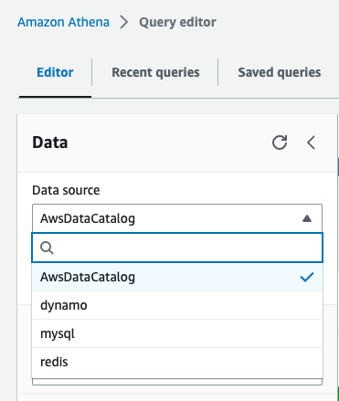
After all four data sources are configured, we can see the data sources on the Data source drop-down menu. All other databases and tables, like the lineitem table, which is stored on Amazon S3, are defined in the AWS Glue Data Catalog and can be accessed by choosing AwsDataCatalog as the data source.
Analyze data with Athena
With our data sources configured, we are ready to start running queries and using federated views in a data mesh architecture. Let’s start by trying to find out how much profit was made on a given line of parts, broken out by supplier nation and year.
For such a query, we need to calculate, for each nation and year, the profit for parts ordered in each year that were filled by a supplier in each nation. Profit is defined as the sum of [(l_extendedprice*(1-l_discount)) - (ps_supplycost * l_quantity)] for all line items describing parts in the specified line.
Answering this question requires querying all four data sources—MySQL, DynamoDB, Redis, and Amazon S3—and is accomplished with the following SQL:
Running this query on the Athena console produces the following result.
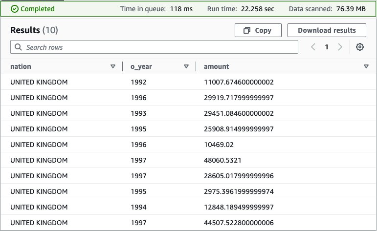
This query is fairly complex: it involves multiple joins and requires special knowledge of the correct way to calculate profit metrics that other end-users may not possess.
To simplify the analysis experience for those users, we can hide this complexity behind a view. For more information on using views with federated data sources, see Querying federated views.
Use the following query to create the view in the data_lake database under the AwsDataCatalog data source:
Next, run a simple select query to validate the view was created successfully: SELECT * FROM federated_view limit 10
The result should be similar to our previous query.
With our view in place, we can perform new analyses to answer questions that would be challenging without the view due to the complex query syntax that would be required. For example, we can find the total profit by nation:
Your results should resemble the following screenshot.
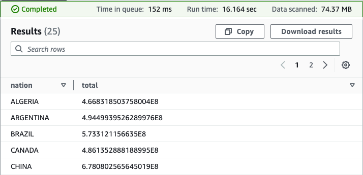
As you now see, the federated view makes it simpler for end-users to run queries on this data. Users are free to query a view of the data, defined by a knowledgeable data producer, rather than having to first acquire expertise in each underlying data source. Because Athena federated queries are processed where the data is stored, with this approach, we avoid duplicating data from the source system, saving valuable time and cost.
Use federated views in a multi-user model
So far, we have satisfied one of the principles of a data mesh: we created a data product (federated view) that is decoupled from its originating source and is available for on-demand analysis by consumers.
Next, we take our data mesh a step further by using federated views in a multi-user model. To keep it simple, assume we have one producer account, the account we used to create our four data sources and federated view, and one consumer account. Using the producer account, we give the consumer account permission to query the federated view from the consumer account.
The following figure depicts this setup and our simplified data mesh architecture.
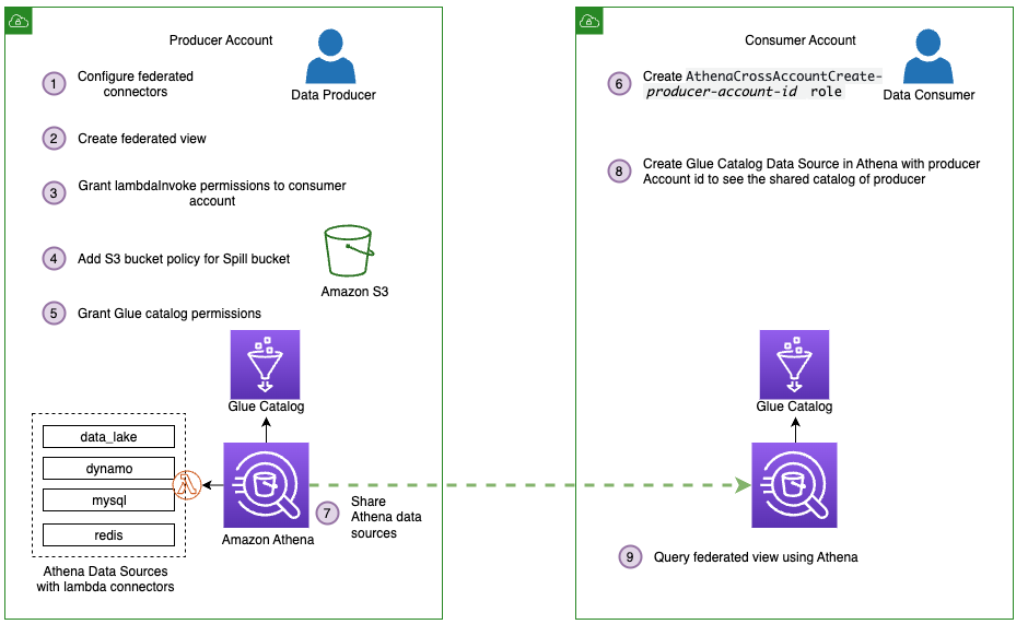
Follow these steps to share the connectors and AWS Glue Data Catalog resources from the producer, which includes our federated view, with the consumer account:
- Share the data sources
mysql,redis,dynamo, anddata_lakewith the consumer account. For instructions, refer to Sharing a data source in Account A with Account B. Note that Account A represents the producer and Account B represents the consumer. Make sure you use the same data source names from earlier when sharing data. This is necessary for the federated view to work in a cross-account model. - Next, share the producer account’s AWS Glue Data Catalog with the consumer account by following the steps in Cross-account access to AWS Glue data catalogs. For the data source name, use
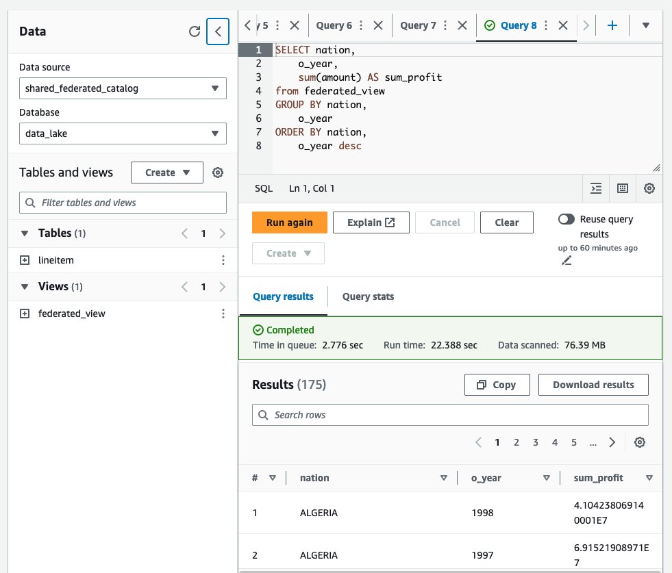
shared_federated_catalog. - Switch to the consumer account, navigate to the Athena console, and verify that you see
federated_viewlisted under Views in theshared_federated_catalogData Catalog anddata_lakedatabase. - Next, run a sample query on the shared view to see the query results.
Clean up
To clean up the resources created for this post, complete the following steps:
- On the Amazon S3 console, empty the bucket
athena-federation-workshop-<account-id>. - If you’re using the AWS CLI, delete the objects in the
athena-federation-workshop-<account-id>bucket with the following code. Make sure you run this command on the correct bucket.
aws s3 rm s3://athena-federation-workshop-<account-id> --recursive - On the AWS CloudFormation console or the AWS CLI, delete the stack
athena-federated-view-blog.
Summary
In this post, we demonstrated the functionality of Athena federated views. We created a view spanning four different federated data sources and ran queries against it. We also saw how federated views could be extended to a multi-user data mesh and ran queries from a consumer account.
To take advantage of federated views, ensure you are using Athena engine version 3 and upgrade your data source connectors to the latest version available. For information on how to upgrade a connector, see Updating a data source connector.
About the Authors
 Saurabh Bhutyani is a Principal Big Data Specialist Solutions Architect at AWS. He is passionate about new technologies. He joined AWS in 2019 and works with customers to provide architectural guidance for running scalable analytics solutions and data mesh architectures using AWS analytics services like Amazon EMR, Amazon Athena, AWS Glue, AWS Lake Formation, and Amazon DataZone.
 Pathik Shah is a Sr. Big Data Architect on Amazon Athena. He joined AWS in 2015 and has been focusing in the big data analytics space since then, helping customers build scalable and robust solutions using AWS analytics services.
Simplify external object access in Amazon Redshift using automatic mounting of the AWS Glue Data Catalog
Post Syndicated from Maneesh Sharma original https://aws.amazon.com/blogs/big-data/simplify-external-object-access-in-amazon-redshift-using-automatic-mounting-of-the-aws-glue-data-catalog/
Amazon Redshift is a petabyte-scale, enterprise-grade cloud data warehouse service delivering the best price-performance. Today, tens of thousands of customers run business-critical workloads on Amazon Redshift to cost-effectively and quickly analyze their data using standard SQL and existing business intelligence (BI) tools.
Amazon Redshift now makes it easier for you to run queries in AWS data lakes by automatically mounting the AWS Glue Data Catalog. You no longer have to create an external schema in Amazon Redshift to use the data lake tables cataloged in the Data Catalog. Now, you can use your AWS Identity and Access Management (IAM) credentials or IAM role to browse the Glue Data Catalog and query data lake tables directly from Amazon Redshift Query Editor v2 or your preferred SQL editors.
This feature is now available in all AWS commercial and US Gov Cloud Regions where Amazon Redshift RA3, Amazon Redshift Serverless, and AWS Glue are available. To learn more about auto-mounting of the Data Catalog in Amazon Redshift, refer to Querying the AWS Glue Data Catalog.
Enabling easy analytics for everyone
Amazon Redshift is helping tens of thousands of customers manage analytics at scale. Amazon Redshift offers a powerful analytics solution that provides access to insights for users of all skill levels. You can take advantage of the following benefits:
- It enables organizations to analyze diverse data sources, including structured, semi-structured, and unstructured data, facilitating comprehensive data exploration
- With its high-performance processing capabilities, Amazon Redshift handles large and complex datasets, ensuring fast query response times and supporting real-time analytics
- Amazon Redshift provides features like Multi-AZ (preview) and cross-Region snapshot copy for high availability and disaster recovery, and provides authentication and authorization mechanisms to make it reliable and secure
- With features like Amazon Redshift ML, it democratizes ML capabilities across a variety of user personas
- The flexibility to utilize different table formats such as Apache Hudi, Delta Lake, and Apache Iceberg (preview) optimizes query performance and storage efficiency
- Integration with advanced analytical tools empowers you to apply sophisticated techniques and build predictive models
- Scalability and elasticity allow for seamless expansion as data and workloads grow
Overall, Amazon Redshift empowers organizations to uncover valuable insights, enhance decision-making, and gain a competitive edge in today’s data-driven landscape.
Amazon Redshift Top Benefits
The new automatic mounting of the AWS Glue Data Catalog feature enables you to directly query AWS Glue objects in Amazon Redshift without the need to create an external schema for each AWS Glue database you want to query. With automatic mounting the Data Catalog, Amazon Redshift automatically mounts the cluster account’s default Data Catalog during boot or user opt-in as an external database, named awsdatacatalog.
Relevant use cases for automatic mounting of the AWS Glue Data Catalog feature
You can use tools like Amazon EMR to create new data lake schemas in various formats, such as Apache Hudi, Delta Lake, and Apache Iceberg (preview). However, when analysts want to run queries against these schemas, it requires administrators to create external schemas for each AWS Glue database in Amazon Redshift. You can now simplify this integration using automatic mounting of the AWS Glue Data Catalog.
The following diagram illustrates this architecture.

Solution overview
You can now use SQL clients like Amazon Redshift Query Editor v2 to browse and query awsdatacatalog. In Query Editor V2, to connect to the awsdatacatalog database, choose the following:
- Must use authentication method Temporary credentials using your IAM identity with the Redshift provisioned cluster
- Must use the authentication method federated user to connect with a Redshift Serverless workgroup.
Complete the following high-level steps to integrate the automatic mounting of the Data Catalog using Query Editor V2 and a third-party SQL client:
- Provision resources with AWS CloudFormation to populate Data Catalog objects.
- Connect Redshift Serverless and query the Data Catalog as a federated user using Query Editor V2.
- Connect with Redshift provisioned cluster and query the Data Catalog using Query Editor V2.
- Configure permissions on catalog resources using AWS Lake Formation.
- Federate with Redshift Serverless and query the Data Catalog using Query Editor V2 and a third-party SQL client.
- Discover the auto-mounted objects.
- Connect with Redshift provisioned cluster and query the Data Catalog as a federated user using a third-party client.
- Connect with Amazon Redshift and query the Data Catalog as an IAM user using third-party clients.
The following diagram illustrates the solution workflow.

Prerequisites
You should have the following prerequisites:
- An AWS account. If you don’t have one, you can sign up for one.
- A Redshift cluster. For setup instructions, see Create a sample Amazon Redshift cluster.
- Alternatively, you could use a Redshift Serverless endpoint. For setup instructions, see Getting started with Amazon Redshift Serverless.
- The latest Amazon Redshift JDBC driver version.
- A SQL client such as SQL workbench/J.
Provision resources with AWS CloudFormation to populate Data Catalog objects
In this post, we use an AWS Glue crawler to create the external table ny_pub stored in Apache Parquet format in the Amazon Simple Storage Service (Amazon S3) location s3://redshift-demos/data/NY-Pub/. In this step, we create the solution resources using AWS CloudFormation to create a stack named CrawlS3Source-NYTaxiData in either us-east-1 (use the yml download or launch stack) or us-west-2 (use the yml download or launch stack). Stack creation performs the following actions:
- Creates the crawler
NYTaxiCrawleralong with the new IAM roleAWSGlueServiceRole-RedshiftAutoMount - Creates
automountdbas the AWS Glue database

When the stack is complete, perform the following steps:
- On the AWS Glue console, under Data Catalog in the navigation pane, choose Crawlers.
- Open
NYTaxiCrawlerand choose Run crawler.

After the crawler is complete, you can see a new table called ny_pub in the Data Catalog under the automountdb database.


Alternatively, you can follow the manual instructions from the Amazon Redshift labs to create the ny_pub table.
Connect with Redshift Serverless and query the Data Catalog as a federated user using Query Editor V2
In this section, we use an IAM role with principal tags to enable fine-grained federated authentication to Redshift Serverless to access auto-mounting AWS Glue objects.
Complete the following steps:
- Create an IAM role and add following permissions. For this post, we add full AWS Glue, Amazon Redshift, and Amazon S3 permissions for demo purposes. In an actual production scenario, it’s recommended to apply more granular permissions.


- On the Tags tab, create a tag with Key as
RedshiftDbRolesand Value asautomount.

- In Query Editor V2, run the following SQL statement as an admin user to create a database role named
automount: - Grant usage privileges to the database role:
- Switch the role to
automountroleby passing the account number and role name.

- In the Query Editor v2, choose your Redshift Serverless endpoint (right-click) and choose Create connection.
- For Authentication, select Federated user.
- For Database, enter the database name you want to connect to.
- Choose Create connection.


You’re now ready to explore and query the automatic mounting of the Data Catalog in Redshift Serverless.

Connect with Redshift provisioned cluster and query the Data Catalog using Query Editor V2
To connect with Redshift provisioned cluster and access the Data Catalog, make sure you have completed the steps in the preceding section. Then complete the following steps:
- Connect to Redshift Query Editor V2 using the database user name and password authentication method. For example, connect to the
devdatabase using the admin user and password. - In an editor tab, assuming the user is present in Amazon Redshift, run the following SQL statement to grant an IAM user access to the Data Catalog:
- As an admin user, choose the Settings icon, choose Account settings, and select Authenticate with IAM credentials.
- Choose Save.

- Switch roles to
automountroleby passing the account number and role name. - Create or edit the connection and use the authentication method Temporary credentials using your IAM identity.

For more information about this authentication method, see Connecting to an Amazon Redshift database.
You are ready to explore and query the automatic mounting of the Data Catalog in Amazon Redshift.

Discover the auto-mounted objects
This section illustrates the SHOW commands for discovery of auto-mounted objects. See the following code:

Configure permissions on catalog resources using AWS Lake Formation
To maintain backward compatibility with AWS Glue, Lake Formation has the following initial security settings:
- The
Superpermission is granted to the groupIAMAllowedPrincipalson all existing Data Catalog resources - The Use only IAM access control setting is enabled for new Data Catalog resources
These settings effectively cause access to Data Catalog resources and Amazon S3 locations to be controlled solely by IAM policies. Individual Lake Formation permissions are not in effect.
In this step, we will configure permissions on catalog resources using AWS Lake Formation. Before you create the Data Catalog, you need to update the default settings of Lake Formation so that access to Data Catalog resources (databases and tables) is managed by Lake Formation permissions:
- Change the default security settings for new resources. For instructions, see Change the default permission model.
- Change the settings for existing Data Catalog resources. For instructions, see Upgrading AWS Glue data permissions to the AWS Lake Formation model.
For more information, refer to Changing the default settings for your data lake.
Federate with Redshift Serverless and query the Data Catalog using Query Editor V2 and a third-party SQL client
With Redshift Serverless, you can connect to awsdatacatalog from a third-party client as a federated user from any identity provider (IdP). In this section, we will configure permission on catalog resources for Federated IAM role in AWS Lake Formation. Using AWS Lake Formation with Redshift, currently permission can be applied on IAM user or IAM role level.
To connect as a federated user, we will be using Redshift Serverless. For setup instructions, refer to Single sign-on with Amazon Redshift Serverless with Okta using Amazon Redshift Query Editor v2 and third-party SQL clients.
There are additional changes required on following resources:
- In Amazon Redshift, as an admin user, grant the usage to each federated user who needs access on
awsdatacatalog:
If the user doesn’t exist in Amazon Redshift, you may need to create the IAM user with the password disabled as shown in the following code and then grant usage on awsdatacatalog:
- On the Lake Formation console, assign permissions on the AWS Glue database to the IAM role that you created as part of the federated setup.
- Under Principals, select IAM users and roles.
- Choose IAM role
oktarole. - Apply catalog resource permissions, selecting
automountdbdatabase and granting appropriate table permissions.

- Update the IAM role used in the federation setup. In addition to the permissions added to the IAM role, you need to add AWS Glue permissions and Amazon S3 permissions to access objects from Amazon S3. For this post, we add full AWS Glue and AWS S3 permissions for demo purposes. In an actual production scenario, it’s recommended to apply more granular permissions.


Now you’re ready to connect to Redshift Serverless using the Query Editor V2 and federated login.
- Use the SSO URL from Okta and log in to your Okta account with your user credentials. For this demo, we log in with user
Ethan. - In the Query Editor v2, choose your Redshift Serverless instance (right-click) and choose Create connection.
- For Authentication, select Federated user.
- For Database, enter the database name you want to connect to.
- Choose Create connection.
- Run the command
select current_userto validate that you are logged in as a federated user.
User Ethan will be able to explore and access awsdatacatalog data.

To connect Redshift Serverless with a third-party client, make sure you have followed all the previous steps.
For SQLWorkbench setup, refer to the section Configure the SQL client (SQL Workbench/J) in Single sign-on with Amazon Redshift Serverless with Okta using Amazon Redshift Query Editor v2 and third-party SQL clients.
The following screenshot shows that federated user ethan is able to query the awsdatacatalog tables using three-part notation:

Connect with Redshift provisioned cluster and query the Data Catalog as a federated user using third-party clients
With Redshift provisioned cluster, you can connect with awsdatacatalog from a third-party client as a federated user from any IdP.
To connect as a federated user with the Redshift provisioned cluster, you need to follow the steps in the previous section that detailed how to connect with Redshift Serverless and query the Data Catalog as a federated user using Query Editor V2 and a third-party SQL client.
There are additional changes required in IAM policy. Update the IAM policy with the following code to use the GetClusterCredentialsWithIAM API:
Now you’re ready to connect to Redshift provisioned cluster using a third-party SQL client as a federated user.
For SQLWorkbench setup, refer to the section Configure the SQL client (SQL Workbench/J) in the post Single sign-on with Amazon Redshift Serverless with Okta using Amazon Redshift Query Editor v2 and third-party SQL clients.
Make the following changes:
- Use the latest Redshift JDBC driver because it only supports querying the auto-mounted Data Catalog table for federated users
- For URL, enter
jdbc:redshift:iam://<cluster endpoint>:<port>:<databasename>?groupfederation=true. For example,jdbc:redshift:iam://redshift-cluster-1.abdef0abc0ab.us-east-2.redshift.amazonaws.com:5439/dev?groupfederation=true.
In the preceding URL, groupfederation is a mandatory parameter that allows you to authenticate with the IAM credentials.

The following screenshot shows that federated user ethan is able to query the awsdatacatalog tables using three-part notation.
Connect and query the Data Catalog as an IAM user using third-party clients
In this section, we provide instructions to set up a SQL client to query the auto-mounted awsdatacatalog.
Use three-part notation to reference the awsdatacatalog table in your SELECT statement. The first part is the database name, the second part is the AWS Glue database name, and the third part is the AWS Glue table name:
You can perform various scenarios that read the Data Catalog data and populate Redshift tables.
For this post, we use SQLWorkbench/J as the SQL client to query the Data Catalog. To set up SQL Workbench/J, complete the following steps:
- Create a new connection in SQL Workbench/J and choose Amazon Redshift as the driver.
- Choose Manage drivers and add all the files from the downloaded AWS JDBC driver pack .zip file (remember to unzip the .zip file).
You must use the latest Redshift JDBC driver because it only supports querying the auto-mounted Data Catalog table.
- For URL, enter
jdbc:redshift:iam://<cluster endpoint>:<port>:<databasename>?profile=<profilename>&groupfederation=true. For example,jdbc:redshift:iam://redshift-cluster-1.abdef0abc0ab.us-east-2.redshift.amazonaws.com:5439/dev?profile=user2&groupfederation=true.

We are using profile-based credentials as an example. You can use any AWS profile or IAM credential-based authentication as per your requirement. For more information on IAM credentials, refer to Options for providing IAM credentials.
The following screenshot shows that IAM user johndoe is able to list the awsdatacatalog tables using the SHOW command.

The following screenshot shows that IAM user johndoe is able to query the awsdatacatalog tables using three-part notation:

If you get the following error while using groupfederation=true, you need to use the latest Redshift driver:
Clean up
Complete the following steps to clean up your resources:
- Delete the IAM role
automountrole. - Delete the CloudFormation stack
CrawlS3Source-NYTaxiDatato clean up the crawlerNYTaxiCrawler, the automountdb database from the Data Catalog, and the IAM roleAWSGlueServiceRole-RedshiftAutoMount.

- Update the default settings of Lake Formation:
- In the navigation pane, under Data catalog, choose Settings.
- Select both access control options choose Save.

- In the navigation pane, under Permissions, choose Administrative roles and tasks.
- In the Database creators section, choose Grant.
- Search for
IAMAllowedPrincipalsand select Create database permission. - Choose Grant.


Considerations
Note the following considerations:
- The Data Catalog auto-mount provides ease of use to analysts or database users. The security setup (setting up the permissions model or data governance) is owned by account and database administrators.
- To achieve fine-grained access control, build a permissions model in AWS Lake Formation.
- If the permissions have to be maintained at the Redshift database level, leave the AWS Lake Formation default settings as is and then run grant/revoke in Amazon Redshift.
- If you are using a third-party SQL editor, and your query tool does not support browsing of multiple databases, you can use the “SHOW“ commands to list your AWS Glue databases and tables. You can also query
awsdatacatalogobjects using three-part notation (SELECT * FROM awsdatacatalog.<aws-glue-db-name>.<aws-glue-table-name>;) provided you have access to the external objects based on the permission model.
Conclusion
In this post, we introduced the automatic mounting of AWS Glue Data Catalog, which makes it easier for customers to run queries in their data lakes. This feature streamlines data governance and access control, eliminating the need to create an external schema in Amazon Redshift to use the data lake tables cataloged in AWS Glue Data Catalog. We showed how you can manage permission on auto-mounted AWS Glue-based objects using Lake Formation. The permission model can be easily managed and organized by administrators, allowing database users to seamlessly access external objects they have been granted access to.
As we strive for enhanced usability in Amazon Redshift, we prioritize unified data governance and fine-grained access control. This feature minimizes manual effort while ensuring the necessary security measures for your organization are in place.
For more information about automatic mounting of the Data Catalog in Amazon Redshift, refer to Querying the AWS Glue Data Catalog.
About the Authors
 Maneesh Sharma is a Senior Database Engineer at AWS with more than a decade of experience designing and implementing large-scale data warehouse and analytics solutions. He collaborates with various Amazon Redshift Partners and customers to drive better integration.
 Debu Panda is a Senior Manager, Product Management at AWS. He is an industry leader in analytics, application platform, and database technologies, and has more than 25 years of experience in the IT world.
 Rohit Vashishtha is a Senior Analytics Specialist Solutions Architect at AWS based in Dallas, Texas. He has 17 years of experience architecting, building, leading, and maintaining big data platforms. Rohit helps customers modernize their analytic workloads using the breadth of AWS services and ensures that customers get the best price/performance with utmost security and data governance.