Post Syndicated from Suvojit Dasgupta original https://aws.amazon.com/blogs/big-data/configure-hadoop-yarn-capacityscheduler-on-amazon-emr-on-amazon-ec2-for-multi-tenant-heterogeneous-workloads/
Apache Hadoop YARN (Yet Another Resource Negotiator) is a cluster resource manager responsible for assigning computational resources (CPU, memory, I/O), and scheduling and monitoring jobs submitted to a Hadoop cluster. This generic framework allows for effective management of cluster resources for distributed data processing frameworks, such as Apache Spark, Apache MapReduce, and Apache Hive. When supported by the framework, Amazon EMR by default uses Hadoop YARN. Please note that not all frameworks offered by Amazon EMR use Hadoop YARN, such as Trino/Presto and Apache HBase.
In this post, we discuss various components of Hadoop YARN, and understand how components interact with each other to allocate resources, schedule applications, and monitor applications. We dive deep into the specific configurations to customize Hadoop YARN’s CapacityScheduler to increase cluster efficiency by allocating resources in a timely and secure manner in a multi-tenant cluster. We take an opinionated look at the configurations for CapacityScheduler and configure them on Amazon EMR on Amazon Elastic Compute Cloud (Amazon EC2) to solve for the common resource allocation, resource contention, and job scheduling challenges in a multi-tenant cluster.
We dive deep into CapacityScheduler because Amazon EMR uses CapacityScheduler by default, and CapacityScheduler has benefits over other schedulers for running workloads with heterogeneous resource consumption.
Solution overview
Modern data platforms often run applications on Amazon EMR with the following characteristics:
- Heterogeneous resource consumption patterns by jobs, such as computation-bound jobs, I/O-bound jobs, or memory-bound jobs
- Multiple teams running jobs with an expectation to receive an agreed-upon share of cluster resources and complete jobs in a timely manner
- Cluster admins often have to cater to one-time requests for running jobs without impacting scheduled jobs
- Cluster admins want to ensure users are using their assigned capacity and not using others
- Cluster admins want to utilize the resources efficiently and allocate all available resources to currently running jobs, but want to retain the ability to reclaim resources automatically should there be a claim for the agreed-upon cluster resources from other jobs
To illustrate these use cases, let’s consider the following scenario:
user1anduser2don’t belong to any team and use cluster resources periodically on an ad hoc basis- A data platform and analytics program has two teams:
- A
data_engineeringteam, containinguser3 - A
data_scienceteam, containinguser4
- A
user5anduser6(and many other users) sporadically use cluster resources to run jobs
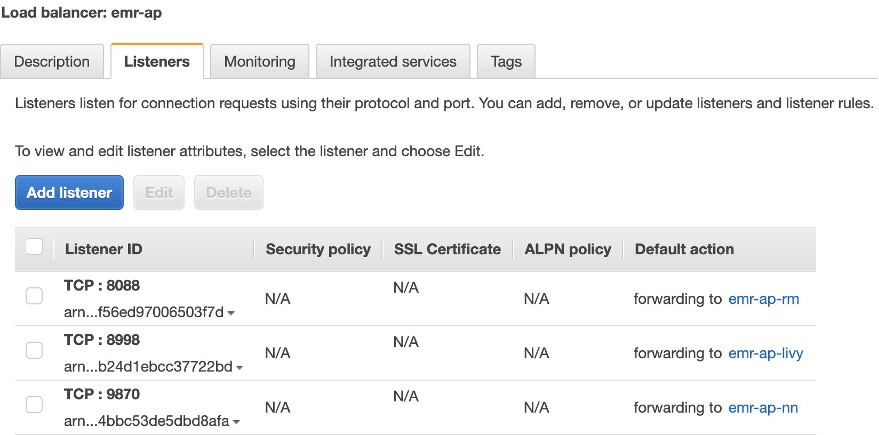
Based on this scenario, the scheduler queue may look like the following diagram. Take note of the common configurations applied to all queues, the overrides, and the user/groups-to-queue mappings.

In the subsequent sections, we will understand the high-level components of Hadoop YARN, discuss the various types of schedulers available in Hadoop YARN, review the core concepts of CapacityScheduler, and showcase how to implement this CapacityScheduler queue setup on Amazon EMR (on Amazon EC2). You can skip to Code walkthrough section if you are already familiar with Hadoop YARN and CapacityScheduler.
Overview of Hadoop YARN
At a high level, Hadoop YARN consists of three main components:
- ResourceManager (one per primary node)
- ApplicationMaster (one per application)
- NodeManager (one per node)
The following diagram shows the main components and their interaction with each other.

Before diving further, let’s clarify what Hadoop YARN’s ResourceContainer (or container) is. A ResourceContainer represents a collection of physical computational resources. It’s an abstraction used to bundle resources into distinct, allocatable unit.
ResourceManager
The ResourceManager is responsible for resource management and making allocation decisions. It’s the ResourceManager’s responsibility to identify and allocate resources to a job upon submission to Hadoop YARN. The ResourceManager has two main components:
- ApplicationsManager (not to be confused with ApplicationMaster)
- Scheduler
ApplicationsManager
The ApplicationsManager is responsible for accepting job submissions, negotiating the first container for running ApplicationMaster, and providing the service for restarting the ApplicationMaster on failure.
Scheduler
The Scheduler is responsible for scheduling allocation of resources to the jobs. The Scheduler performs its scheduling function based on the resource requirements of the jobs. The Scheduler is a pluggable interface. Hadoop YARN currently provides three implementations:
- CapacityScheduler – A pluggable scheduler for Hadoop that allows for multiple tenants to securely share a cluster such that jobs are allocated resources in a timely manner under constraints of allocated capacities. The implementation is available on GitHub. The Java concrete class is
org.apache.hadoop.yarn.server.resourcemanager.scheduler.capacity.CapacityScheduler. In this post, we primarily focus on CapacityScheduler, which is the default scheduler on Amazon EMR (on Amazon EC2). - FairScheduler – A pluggable scheduler for Hadoop that allows Hadoop YARN applications to share resources in clusters fairly. The implementation is available on GitHub. The Java concrete class is
org.apache.hadoop.yarn.server.resourcemanager.scheduler.fair.FairScheduler. - FifoScheduler – A pluggable scheduler for Hadoop that allows Hadoop YARN applications share resources in clusters in a first-in-first-out basis. The implementation is available on GitHub. The Java concrete class is
org.apache.hadoop.yarn.server.resourcemanager.scheduler.fifo.FifoScheduler.
ApplicationMaster
Upon negotiating the first container by ApplicationsManager, the per-application ApplicationMaster has the responsibility of negotiating the rest of the appropriate resources from the Scheduler, tracking their status, and monitoring progress.
NodeManager
The NodeManager is responsible for launching and managing containers on a node.
Hadoop YARN on Amazon EMR
By default, Amazon EMR (on Amazon EC2) uses Hadoop YARN for cluster management for the distributed data processing frameworks that support Hadoop YARN as a resource manager, like Apache Spark, Apache MapReduce, and Apache Hive. Amazon EMR provides multiple sensible default settings that work for most scenarios. However, every data platform is different and has specific needs. Amazon EMR provides the ability to customize the setting at cluster creation using configuration classifications . You can also reconfigure Amazon EMR cluster applications and specify additional configuration classifications for each instance group in a running cluster using AWS Command Line Interface (AWS CLI), or the AWS SDK.
CapacityScheduler
CapacityScheduler depends on ResourceCalculator to identify the available resources and calculate the allocation of the resources to ApplicationMaster. The ResourceCalculator is an abstract Java class. Hadoop YARN currently provides two implementations:
- DefaultResourceCalculator – In
DefaultResourceCalculator, resources are calculated based on memory alone. - DominantResourceCalculator –
DominantResourceCalculatoris based on the Dominant Resource Fairness (DRF) model of resource allocation. The paper Dominant Resource Fairness: Fair Allocation of Multiple Resource Types, Ghodsi et al. [2011] describes DRF as follows: “DRF computes the share of each resource allocated to that user. The maximum among all shares of a user is called that user’s dominant share, and the resource corresponding to the dominant share is called the dominant resource. Different users may have different dominant resources. For example, the dominant resource of a user running a computation-bound job is CPU, while the dominant resource of a user running an I/O-bound job is bandwidth. DRF simply applies max-min fairness across users’ dominant shares. That is, DRF seeks to maximize the smallest dominant share in the system, then the second-smallest, and so on.”
Because of DRF, DominantResourceCalculator is a better ResourceCalculator for data processing environments running heterogeneous workloads. By default, Amazon EMR uses DefaultResourceCalculator for CapacityScheduler. This can be verified by checking the value of yarn.scheduler.capacity.resource-calculator parameter in /etc/hadoop/conf/capacity-scheduler.xml.
Code walkthrough
CapacityScheduler provides multiple parameters to customize the scheduling behavior to meet specific needs. For a list of available parameters, refer to Hadoop: CapacityScheduler.
Refer to the configurations section in cloudformation/templates/emr.yaml to review all the CapacityScheduler parameters set as part of this post. In this example, we use two classifiers of Amazon EMR (on Amazon EC2):
- yarn-site – The classification to update
yarn-site.xml - capacity-scheduler – The classification to update
capacity-scheduler.xml
For various types of classification available in Amazon EMR, refer to Customizing cluster and application configuration with earlier AMI versions of Amazon EMR.
In the AWS CloudFormation template, we have modified the ResourceCalculator of CapacityScheduler from the defaults, DefaultResourceCalculator to DominantResourceCalculator. Data processing environments tends to run different kinds of jobs, for example, computation-bound jobs consuming heavy CPU, I/O-bound jobs consuming heavy bandwidth, and memory-bound jobs consuming heavy memory. As previously stated, DominantResourceCalculator is better suited for such environments due to its Dominant Resource Fairness model of resource allocation. If your data processing environment only runs memory-bound jobs, then modifying this parameter isn’t necessary.
You can find the codebase in the AWS Samples GitHub repository.
Prerequisites
For deploying the solution, you should have the following prerequisites:
- An AWS account
- The AWS Command Line Interface (AWS CLI) installed
- The GIT Command Line Interface (GIT CLI) installed
- Permission to create AWS resources
- Familiarity with AWS CloudFormation and Amazon EMR
Deploy the solution
To deploy the solution, complete the following steps:
- Download the source code from the AWS Samples GitHub repository:
- Create an Amazon Simple Storage Service (Amazon S3) bucket:
- Copy the cloned repository to the Amazon S3 bucket:
- Update the amazon-emr-yarn-capacity-scheduler/cloudformation/parameters/parameters.json file with appropriate values for the following keys. We have provided sensible defaults wherever possible. You should update the values to fit your specific requirements.
-
- ArtifactsS3Repository – The S3 bucket name that was created in the previous step (
emr-yarn-capacity-scheduler-<AWS_ACCOUNT_ID>-<AWS_REGION>). - emrKeyName – An existing EC2 key name. If you don’t have an existing key and want to create a new key, refer to Use an Amazon EC2 key pair for SSH credentials.
- clientCIDR – The CIDR range of the client machine for accessing the EMR cluster via SSH. You can run the following command to identify the IP of the client machine:
echo "$(curl -s http://checkip.amazonaws.com)/32"
- ArtifactsS3Repository – The S3 bucket name that was created in the previous step (
- Deploy the AWS CloudFormation templates:
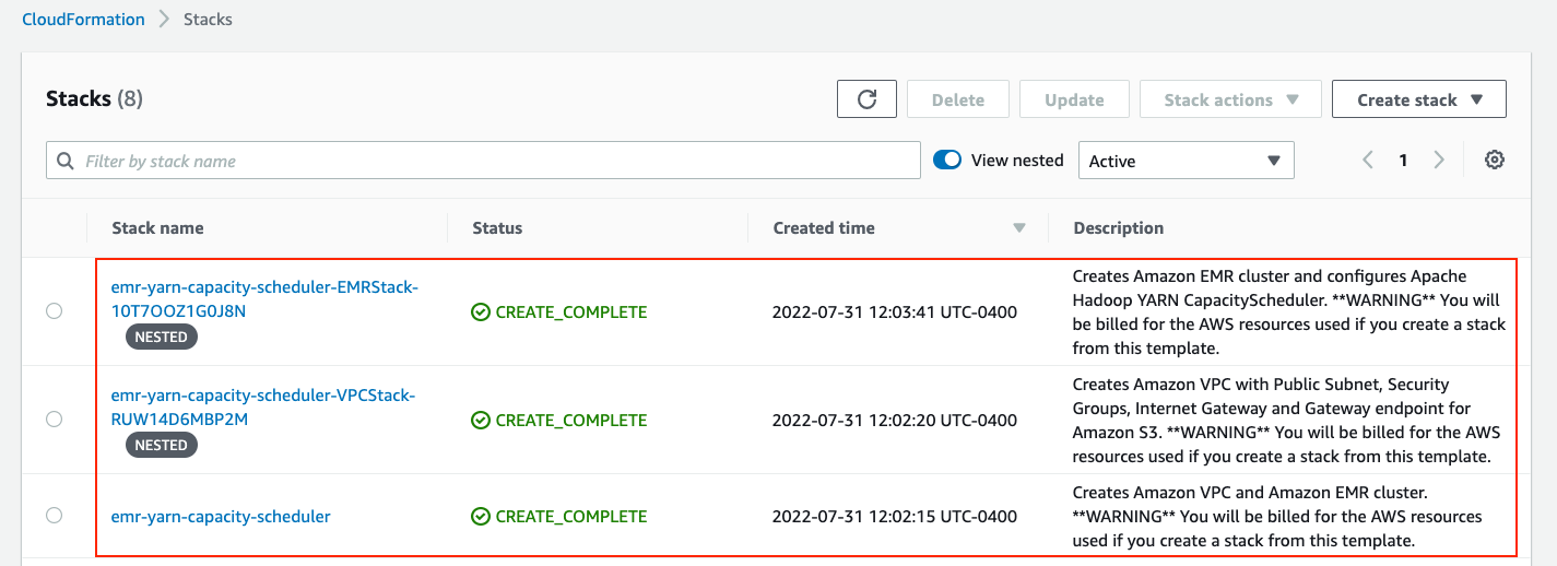
- On the AWS CloudFormation console, check for the successful deployment of the following stacks.
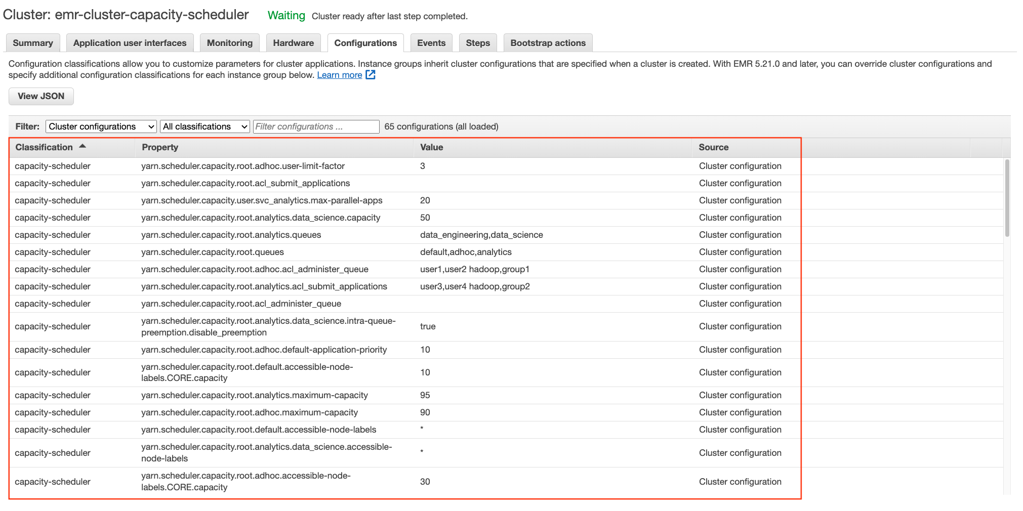
- On the Amazon EMR console, check for the successful creation of the
emr-cluster-capacity-schedulercluster. - Choose the cluster and on the Configurations tab, review the properties under the
capacity-schedulerandyarn-siteclassification labels.
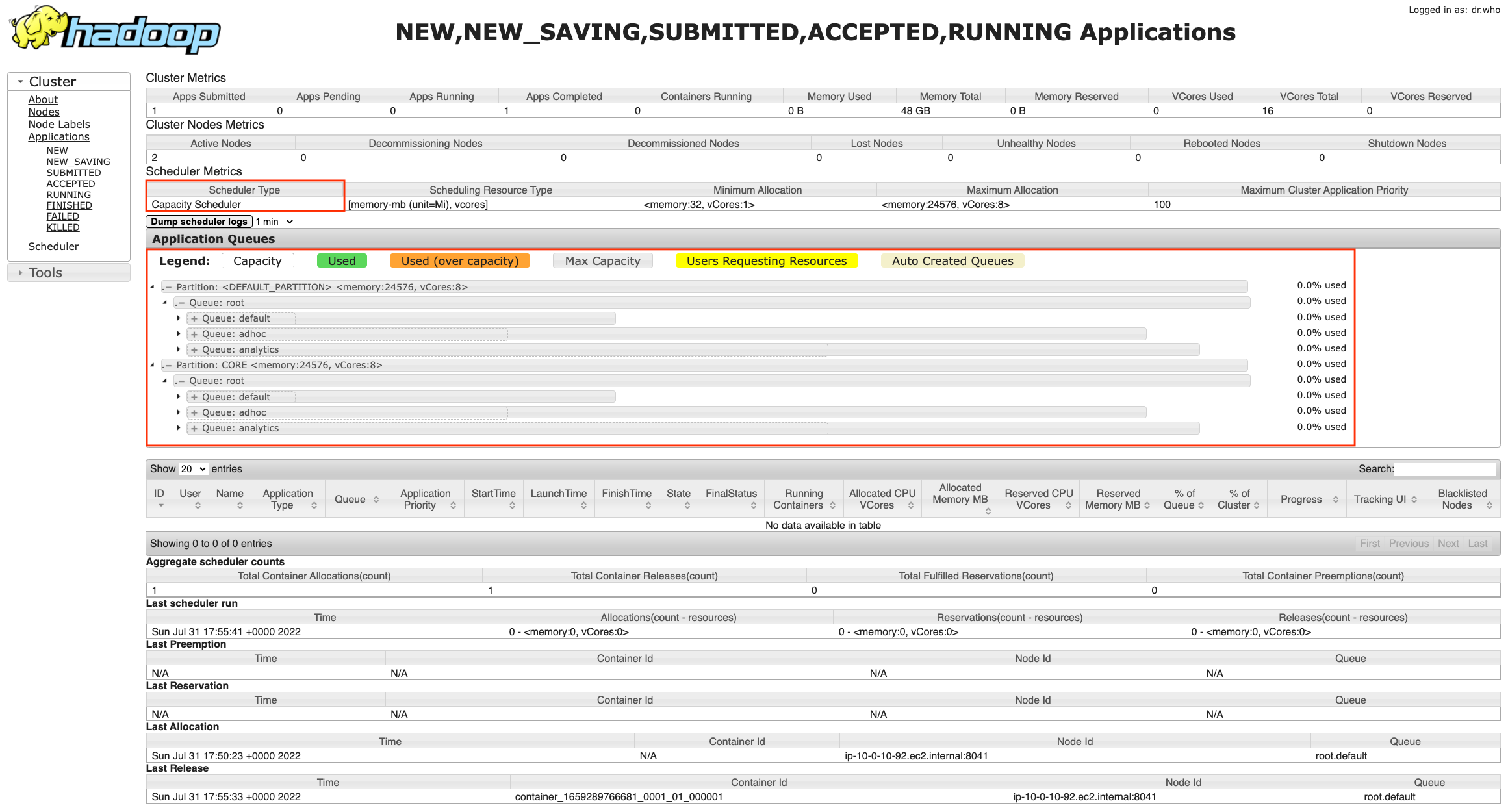
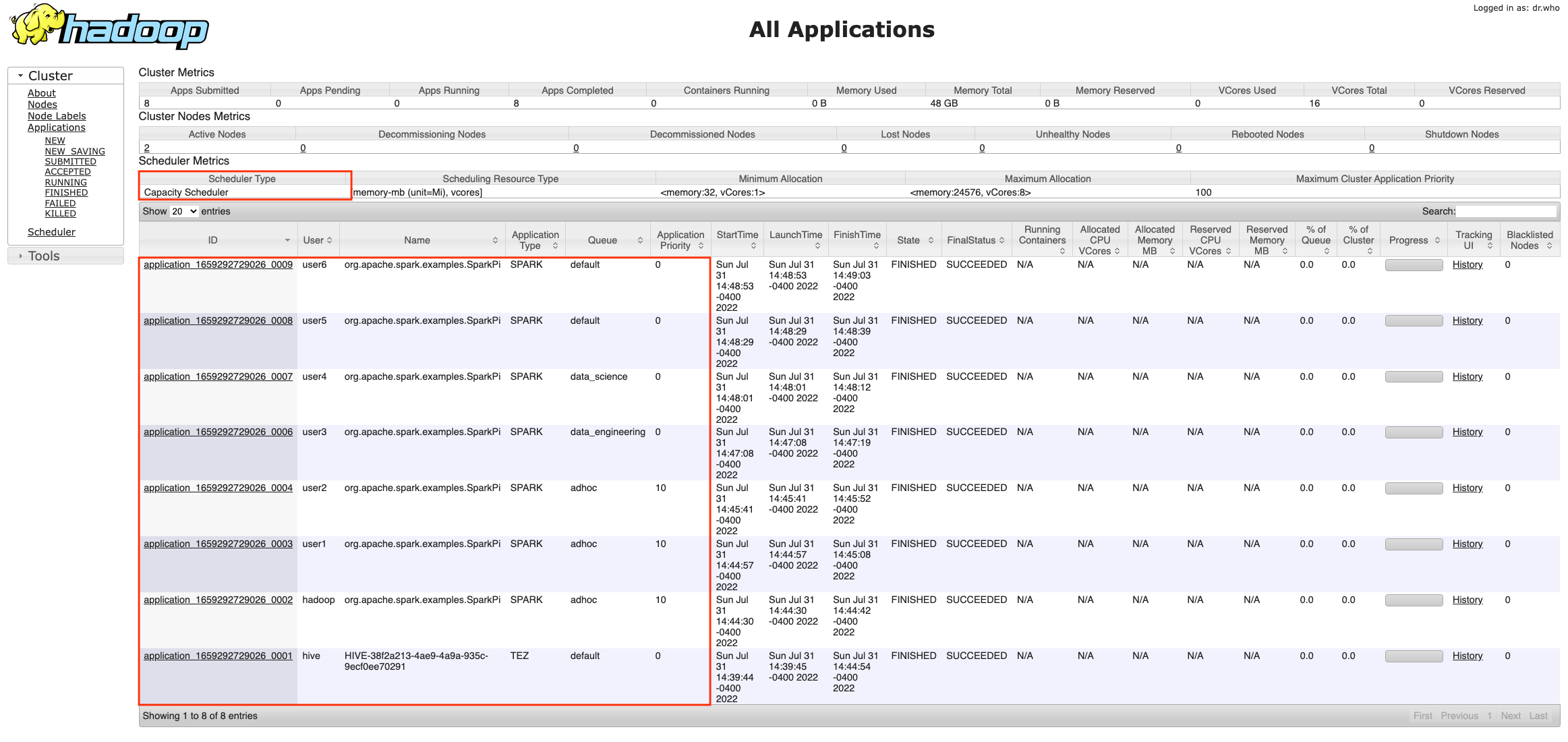
- Access the Hadoop YARN resource manager UI on the
emr-cluster-capacity-schedulercluster to review the CapacityScheduler setup. For instructions on how to access the UI on Amazon EMR, refer to View web interfaces hosted on Amazon EMR clusters.
- SSH into the
emr-cluster-capacity-schedulercluster and review the following files.For instructions on how to SSH into the EMR primary node, refer to Connect to the master node using SSH.
-
/etc/hadoop/conf/yarn-site.xml/etc/hadoop/conf/capacity-scheduler.xml
All the parameters set using the yarn-site and capacity-scheduler classifiers are reflected in these files. If an admin wants to update CapacityScheduler configs, they can directly update capacity-scheduler.xml and run the following command to apply the changes without interrupting any running jobs and services:
Changes to yarn-site.xml require the ResourceManager service to be restarted, which interrupts the running jobs. As a best practice, refrain from manual modifications and use version control for change management.
The CloudFormation template adds a bootstrap action to create test users (user1, user2, user3, user4, user5 and user6) on all the nodes and adds a step script to create HDFS directories for the test users.
Users can SSH into the primary node, sudo as different users and submit Spark jobs to verify the job submission and CapacityScheduler behavior:
You can validate the results from the resource manager web UI.
Clean up
To avoid incurring future charges, delete the resources you created.
- Delete the CloudFormation stack:
- Delete the S3 bucket:
The command deletes the bucket and all files underneath it. The files may not be recoverable after deletion.
Conclusion
In this post, we discussed Apache Hadoop YARN and its various components. We discussed the types of schedulers available in Hadoop YARN. We dived deep in to the specifics of Hadoop YARN CapacityScheduler and the use of Dominant Resource Fairness to efficiently allocate resources to submitted jobs. We also showcased how to implement the discussed concepts using AWS CloudFormation.
We encourage you to use this post as a starting point to implement CapacityScheduler on Amazon EMR (on Amazon EC2) and customize the solution to meet your specific data platform goals.
About the authors
![]() Suvojit Dasgupta is a Sr. Lakehouse Architect at Amazon Web Services. He works with customers to design and build data solutions on AWS.
Suvojit Dasgupta is a Sr. Lakehouse Architect at Amazon Web Services. He works with customers to design and build data solutions on AWS.
![]() Bharat Gamini is a Data Architect focused on big data and analytics at Amazon Web Services. He helps customers architect and build highly scalable, robust, and secure cloud-based analytical solutions on AWS.
Bharat Gamini is a Data Architect focused on big data and analytics at Amazon Web Services. He helps customers architect and build highly scalable, robust, and secure cloud-based analytical solutions on AWS.
 Melody Yang is a Senior Big Data Solution Architect for Amazon EMR at AWS. She is an experienced analytics leader working with AWS customers to provide best practice guidance and technical advice in order to assist their success in data transformation. Her areas of interests are open-source frameworks and automation, data engineering and DataOps.


 Bharat Gamini is a Data Architect focused on Big Data & Analytics at Amazon Web Services. He helps customers architect and build highly scalable, robust and secure cloud-based analytical solutions on AWS.
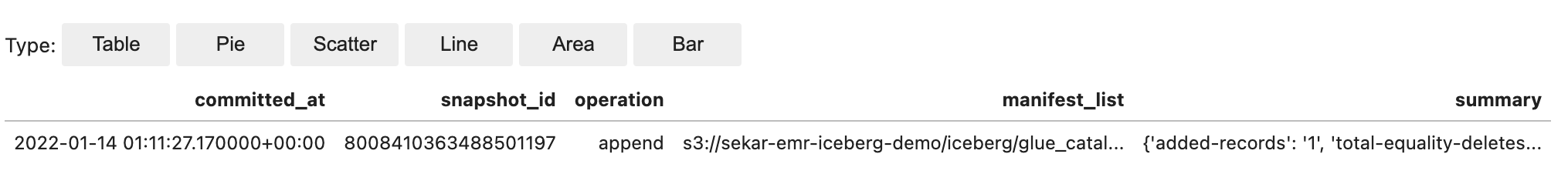


 We also have more


 Bharath Kumar Boggarapu is a Data Architect at AWS Professional Services with expertise in big data technologies. He is passionate about helping customers build performant and robust data-driven solutions and realize their data and analytics potential. His areas of interests are open-source frameworks, automation, and data architecting. In his free time, he loves to spend time with family, play tennis, and travel.


 John Benninghoff is a AWS Professional Services Sr. Data Architect, focused on Data Lake architecture and implementation.