Tag Archives: Amazon OpenSearch Service

AWS Weekly Review: Amazon EKS, Amazon OpenSearch, Amazon API Gateway, and more (April 7, 2025)

Post Syndicated from Sébastien Stormacq original https://aws.amazon.com/blogs/aws/aws-weekly-review-amazon-eks-amazon-opensearch-amazon-api-gateway-and-more-april-7-2025/

AWS Summit season starts this week! These free events are now rolling out worldwide, bringing our cloud computing community together to connect, collaborate, and learn. Whether you prefer joining us online or in-person, these gatherings offer valuable opportunities to expand your AWS knowledge. I will be attending the Summit in Paris this week, the biggest cloud conference in France, and the London Summit at the end of the month. We will have a small podcast recording studio where I will interview French and British customers to produce new episodes for the AWS Developers Podcast and le podcast 🎙 AWS ☁ en 🇫🇷.

Register today!

But for now, let’s look at last week’s new announcements.

Last week’s launches
At KubeCon London, we introduced the EKS Community Add-Ons Catalog, making it simpler for Kubernetes users to enhance their Amazon EKS clusters with powerful open-source tools. This catalog streamlines the installation of essential add-ons like metrics-serverkube-state-metricsprometheus-node-exportercert-manager, and external-dns. By integrating these community-driven add-ons directly into the EKS console and AWS command line interface (AWS CLI), customers can reduce operational complexity and accelerate deployment while maintaining flexibility and security. This launch reflects AWS’s commitment to the Kubernetes community, providing seamless access to trusted open-source solutions without the overhead of manual installation and maintenance.

Amazon Q Developer now integrates with Amazon OpenSearch Service to enhance operational analytics by enabling natural language exploration and AI-assisted data visualization. This integration simplifies the process of querying and visualizing operational data, reducing the learning curve associated with traditional query languages and tools. During incident responses, Amazon Q Developer offers contextual summaries and insights directly within the alerts interface, facilitating quicker analysis and resolution. This advancement allows engineers to focus more on innovation by streamlining troubleshooting processes and improving monitoring infrastructure.

Amazon API Gateway now supports dual-stack (IPv4 and IPv6) endpoints across all endpoint types, custom domains, and management APIs in both commercial and AWS GovCloud (US) Regions. This enhancement allows REST, HTTP, and WebSocket APIs, as well as custom domains, to handle requests from both IPv4 and IPv6 clients, facilitating a smoother transition to IPv6 and addressing IPv4 address scarcity. Additionally, AWS continues its commitment to IPv6 adoption with recent updates, including AWS Identity and Access Management (IAM) introducing dual-stack public endpoints for seamless connections over IPv4 and IPv6, and AWS Resource Access Manager (RAM) enabling customers to manage resource shares using IPv6 addresses. Amazon Security Lake customers can also now use Internet Protocol version 6 (IPv6) addresses via new dual-stack endpoints to configure and manage the service. These advancements collectively ensure broader compatibility and future-proofing of network infrastructure.

Amazon SES has introduced support for email attachments in its v2 APIs, enabling users to include files like PDFs and images directly in their emails without manually constructing MIME messages. This enhancement simplifies the process of sending rich email content and reduces implementation complexity. Amazon Simple Email Service (Amazon SES) supports attachments in all AWS Regions where the service is available.

Amazon Neptune has updated its Service Level Agreement (SLA) to offer a 99.99% Monthly Uptime Percentage for Multi-AZ DB Instance, Multi-AZ DB Cluster, and Multi-AZ Graph configurations, up from the previous 99.9%. This enhancement demonstrates the commitment AWS has to providing highly available and reliable graph database services for mission-critical applications. The improved SLA is now available in all AWS Regions where Amazon Neptune is offered.

For a full list of AWS announcements, be sure to keep an eye on the What’s New at AWS page.

Other AWS events
Check your calendar and sign up for upcoming AWS events.

AWS GenAI Lofts are collaborative spaces and immersive experiences that showcase AWS expertise in cloud computing and AI. They provide startups and developers with hands-on access to AI products and services, exclusive sessions with industry leaders, and valuable networking opportunities with investors and peers. Find a GenAI Loft location near you and don’t forget to register.

Browse all upcoming AWS led in-person and virtual events here.

That’s all for this week. Check back next Monday for another Weekly Roundup!

— seb

This post is part of our Weekly Roundup series. Check back each week for a quick roundup of interesting news and announcements from AWS!


How is the News Blog doing? Take this 1 minute survey!

(This survey is hosted by an external company. AWS handles your information as described in the AWS Privacy Notice. AWS will own the data gathered via this survey and will not share the information collected with survey respondents.)

Optimize multimodal search using the TwelveLabs Embed API and Amazon OpenSearch Service

Post Syndicated from James Le original https://aws.amazon.com/blogs/big-data/optimize-multimodal-search-using-the-twelvelabs-embed-api-and-amazon-opensearch-service/

This blog is co-authored by James Le, Head of Developer Experience – TwelveLabs

The exponential growth of video content has created both opportunities and challenges. Content creators, marketers, and researchers are now faced with the daunting task of efficiently searching, analyzing, and extracting valuable insights from vast video libraries. Traditional search methods such as keyword-based text search often fall short when dealing with video content to analyze the visual content, spoken words, or contextual elements within the video itself, leaving organizations struggling to effectively search through and unlock the full potential of their multimedia assets.

With the integration of TwelveLabs’ Embed API and Amazon OpenSearch Service, we can interact with and derive value from video content. By using TwelveLabs‘ advanced AI-powered video understanding technology and OpenSearch Service’s search and analytics capabilities, we can now perform advanced video discovery and gain deeper insights.

In this blog post, we show you the process of integrating TwelveLabs Embed API with OpenSearch Service to create a multimodal search solution. You’ll learn how to generate rich, contextual embeddings from video content and use OpenSearch Service’s vector database capabilities to enable search functionalities. By the end of this post, you’ll be equipped with the knowledge to implement a system that can transform the way your organization handles and extracts value from video content.

TwelveLabs’ multimodal embeddings process visual, audio, and text signals together to create unified representations, capturing the direct relationships between these modalities. This unified approach delivers precise, context-aware video search that matches human understanding of video content. Whether you’re a developer looking to enhance your applications with advanced video search capabilities, or a business leader seeking to optimize your content management strategies, this post will provide you with the tools and steps to implement multimodal search for your organizational data.

About TwelveLabs

TwelveLabs is an Advanced AWS Partner and AWS Marketplace Seller that offers video understanding solutions. Embed API is designed to revolutionize how you interact with and extract value from video content.

At its core, the Embed API transforms raw video content into meaningful, searchable data by using state-of-the-art machine learning models. These models extract and represent complex video information in the form of dense vector embeddings, each a standard 1024-dimensional vector that captures the essence of the video content across multiple modalities (image, text, and audio).

Key features of TwelveLabs Embed API

Below are the key features of TwelveLabs Embed API:

  • Multimodal understanding: The API generates embeddings that encapsulate various aspects of the video, including visual expressions, body language, spoken words, and overall context.
  • Temporal coherence: Unlike static image-based models, TwelveLabs’ embeddings capture the interrelations between different modalities over time, providing a more accurate representation of video content.
  • Flexibility: The API supports native processing of all modalities present in videos, eliminating the need for separate text-only or image-only models.
  • High performance: By using a video-native approach, the Embed API provides more accurate and temporally coherent interpretation of video content compared to traditional CLIP-like models.

Benefits and use cases

The Embed API offers numerous advantages for developers and businesses working with video content:

  • Enhanced Search Capabilities: Enable powerful multimodal search across video libraries, allowing users to find relevant content based on visual, audio, or textual queries.
  • Content Recommendation: Improve content recommendation systems by understanding the deep contextual similarities between videos.
  • Scene Detection and Segmentation: Automatically detect and segment different scenes within videos for easier navigation and analysis.
  • Content Moderation: Efficiently identify and flag inappropriate content across large video datasets.

Use cases include:

  • Anomaly detection
  • Diversity sorting
  • Sentiment analysis
  • Recommendations

Architecture overview

The architecture for using TwelveLabs Embed API and OpenSearch Service for advanced video search consists of the following components:

  • TwelveLabs Embed API: This API generates 1024-dimensional vector embeddings from video content, capturing visual, audio, and textual elements.
  • OpenSearch Vector Database: Stores and indexes the video embeddings generated by TwelveLabs.
  • Secrets Manager to store secrets such as API access keys, and the Amazon OpenSearch Service username and password.
  • Integration of TwelveLabs SDK and the OpenSearch Service client to process videos, generate embeddings, and index them in OpenSearch Service.

The following diagram illustrates:

  1. A video file is stored in Amazon Simple Storage Service (Amazon S3). Embeddings of the video file are created using TwelveLabs Embed API.
  2. Embeddings generated from the TwelveLabs Embed API are now ingested to Amazon OpenSearch Service.
  3. Users can search the video embeddings using text, audio, or image. The user uses TwelveLabs Embed API to create the corresponding embeddings.
  4. The user searches video embeddings in Amazon OpenSearch Service and retrieves the corresponding vector.

The use case

For the demo, you will work on these videos: Robin bird forest Video by Federico Maderno from Pixabay and Island Video by Bellergy RC from Pixabay.

However, the use case can be expanded to various other segments. For example, the news organization struggles with:

  1. Needle-in-haystack searches through thousands of hours of archival footage
  2. Manual metadata tagging that misses nuanced visual and audio context
  3. Cross-modal queries such as querying a video collection using text or audio descriptions
  4. Rapid content retrieval for breaking news tie-ins

By integrating TwelveLabs Embed API with OpenSearch Service, you can:

  • Generate 1024-dimensional embeddings capturing each video’s visual concepts. The embeddings are also capable of extracting spoken narration, on-screen text, and audio cues.
  • Enable multimodal search capabilities allowing users to:
    • Find specific demonstrations using text-based queries.
    • Locate activities through image-based queries.
    • Identify segments using audio pattern matching.
  • Reduce search time from hours to seconds for complex queries.

Solution walkthrough

GitHub repository contains a notebook with detailed walkthrough instructions for implementing advanced video search capabilities by combining TwelveLabs’ Embed API with Amazon OpenSearch Service.

Prerequisites

Before you proceed further, verify that the following prerequisites are met:

  • Confirm that you have an AWS account. Sign in to the AWS account.
  • Create a TwelveLabs account because it will be required to get the API Key. TwelveLabs offer free tier pricing but you can upgrade if necessary to meet your requirement.
  • Have an Amazon OpenSearch Service domain. If you don’t have an existing domain, you can create one using the steps outlined in our public documentation for Creating and Managing Amazon OpenSearch Service Domain. Make sure that the OpenSearch Service domain is accessible from your Python environment. You can also use Amazon OpenSearch Serverless for this use case and update the interactions to OpenSearch Serverless using AWS SDKs.

Step 1: Set up the TwelveLabs SDK

Start by setting up the TwelveLabs SDK in your Python environment:

  1. Obtain your API key from TwelveLabs Dashboard.
  2. Follow steps here to create a secret in AWS Secrets Manager. For example, name the secret as TL_API_Key.Note down the ARN or name of the secret (TL_API_Key) to retrieve. To retrieve a secret from another account, you must use an ARN.For an ARN, we recommend that you specify a complete ARN rather than a partial ARN. See Finding a secret from a partial ARN.Use this value for the SecretId in the code block below.
import boto3
import json
secrets_manager_client=boto3.client("secretsmanager")
API_secret=secrets_manager_client.get_secret_value(
SecretId="TL_API_KEY"
)
TL_API_KEY=json.loads(API_secret["SecretString"])["TL_API_Key"]

Step 2: Generate video embeddings

Use the Embed API to create multimodal embeddings that are contextual vector representations for your videos and texts. TwelveLabs video embeddings capture all the subtle cues and interactions between different modalities, including the visual expressions, body language, spoken words, and the overall context of the video, encapsulating the essence of all these modalities and their interrelations over time.

To create video embeddings, you must first upload your videos, and the platform must finish processing them. Uploading and processing videos require some time. Consequently, creating embeddings is an asynchronous process comprised of three steps:

  1. Upload and process a video: When you start uploading a video, the platform creates a video embedding task and returns its unique task identifier.
  2. Monitor the status of your video embedding task: Use the unique identifier of your task to check its status periodically until it’s completed.
  3. Retrieve the embeddings: After the video embedding task is completed, retrieve the video embeddings by providing the task identifier. Learn more in the docs.

Video processing implementation

This demo depends upon some video data. To use this, you will download two mp4 files and upload it to an Amazon S3 bucket.

  1. Click on the links containing the Robin bird forest Video by Federico Maderno from Pixabay and Island Video by Bellergy RC from Pixabay videos.
  2. Download the 21723-320725678_small.mp4 and 2946-164933125_small.mp4 files.
  3. Create an S3 bucket if you don’t have one already. Follow the steps in the Creating a bucket doc. Note down the name of the bucket and replace it the code block below (Eg., MYS3BUCKET).
  4. Upload the 21723-320725678_small.mp4 and 2946-164933125_small.mp4 video files to the S3 bucket created in the step above by following the steps in the Uploading objects doc. Note down the name of the objects and replace it the code block below (Eg., 21723-320725678_small.mp4 and 2946-164933125_small.mp4)
s3_client=boto3.client("s3")
bird_video_data=s3_client.download_file(Bucket='MYS3BUCKET',  Key='21723-320725678_small.mp4', Filename='robin-bird.mp4')
island_video_data=s3_client.download_file(Bucket='MYS3BUCKET',  Key='2946-164933125_small.mp4', Filename='island.mp4')

def print_segments(segments: List[SegmentEmbedding], max_elements: int = 1024):
    for segment in segments:
        print(
            f"  embedding_scope={segment.embedding_scope} start_offset_sec={segment.start_offset_sec} end_offset_sec={segment.end_offset_sec}"
        )
        print(f"  embeddings: {segment.embeddings_float[:max_elements]}")

# Initialize client with API key
twelvelabs_client = TwelveLabs(api_key=TL_API_KEY)

video_files=["robin-bird.mp4", "island.mp4"]
tasks=[]

Embedding generation process

With the SDK configured, generate embeddings for your video and monitor task completion with real-time updates. Here you use the Marengo 2.7 model to generate the embeddings:

for video in video_files:
    # Create embedding task
    task = twelvelabs_client.embed.task.create(
        model_name="Marengo-retrieval-2.7",
        video_file=video
    )
    print(
        f"Created task: id={task.id} engine_name={task.model_name} status={task.status}"
    )
    
    def on_task_update(task: EmbeddingsTask):
        print(f"  Status={task.status}")
    
    status = task.wait_for_done(
        sleep_interval=2,
        callback=on_task_update
    )
    print(f"Embedding done: {status}")
    
    # Retrieve and inspect results
    task = task.retrieve()
    if task.video_embedding is not None and task.video_embedding.segments is not None:
        print_segments(task.video_embedding.segments)
    tasks.append(task)

Key features demonstrated include:

  • Multimodal capture: 1024-dimensional vectors encoding visual, audio, and textual features
  • Model specificity: Using Marengo-retrieval-2.7 optimized for scientific content
  • Progress tracking: Real-time status updates during embedding generation

Expected output

Created task: id=67ca93a989d8a564e80dc3ba engine_name=Marengo-retrieval-2.7 status=processing
  Status=processing
  Status=processing
  Status=processing
  Status=processing
  Status=processing
  Status=processing
  Status=processing
  Status=processing
  Status=processing
  Status=ready
Embedding done: ready
  embedding_scope=clip start_offset_sec=0.0 end_offset_sec=6.0
  embeddings: [0.022429451, 0.00040668788, -0.01825908, -0.005862708, -0.03371106, 
-6.357456e-05, -0.015320076, -0.042556215, -0.02782445, -0.00019097517, 0.03258314, 
-0.0061399476, -0.00049206393, 0.035632476, 0.028209884, 0.02875258, -0.035486065, 
-0.11288028, -0.040782217, -0.0359422, 0.015908664, -0.021092793, 0.016303983, 
0.06351931,…………………

Step 3: Set up OpenSearch

To enable vector search capabilities, you first need to set up an OpenSearch client and test the connection. Follow these steps:

Install the required libraries

Install the necessary Python packages for working with OpenSearch:

!pip install opensearch-py
!pip install botocore
!pip install requests-aws4auth

Configure the OpenSearch client

Set up the OpenSearch client with your host details and authentication credentials:

from opensearchpy import OpenSearch, RequestsHttpConnection, helpers
from requests_aws4auth import AWS4Auth
from requests.auth import HTTPBasicAuth

# OpenSearch connection configuration
# host = 'your-host.aos.us-east-1.on.aws'
host = 'search-new-domain-mbgs7wth6r5w6hwmjofntiqcge.aos.us-east-1.on.aws'
port = 443  # Default HTTPS port

# Get OpenSearch username secret from Secrets Manager
opensearch_username=secrets_manager_client.get_secret_value(
    SecretId="AOS_username"
)
opensearch_username_string=json.loads(opensearch_username["SecretString"])["AOS_username"]

# Get OpenSearch password secret from Secrets Manager
opensearch_password = secrets_manager_client.get_secret_value(
    SecretId="AOS_password"
)
opensearch_password_string=json.loads(opensearch_password["SecretString"])["AOS_password"]

auth=(opensearch_username_string, opensearch_password_string)

# Create the client configuration
client_aos = OpenSearch(
    hosts=[{'host': host, 'port': port}],
    http_auth=auth,
    use_ssl=True,
    verify_certs=True,
    connection_class=RequestsHttpConnection
)

# Test the connection
try:
    # Get cluster information
    cluster_info = client_aos.info()
    print("Successfully connected to OpenSearch")
    print(f"Cluster info: {cluster_info}")
except Exception as e:
    print(f"Connection failed: {str(e)}")

Expected output

If the connection is successful, you should see a message like the following:

Successfully connected to OpenSearch
Cluster info: {'name': 'bb36e8d98ee7bd517891ecd714bfb9d7', ...}

This confirms that your OpenSearch client is properly configured and ready for use.

Step 4: Create an index in OpenSearch Service

Next, you create an index optimized for vector search to store the embeddings generated by the TwelveLabs Embed API.

Define the index configuration

The index is configured to support k-nearest neighbor (kNN) search with a 1024-dimensional vector field. You will these values for this demo but follow these best practices to find appropriate values for your application. Here’s the code:

# Define the enhanced index configuration
index_name = 'twelvelabs_index'
new_vector_index_definition = {
    "settings": {
        "index": {
            "knn": "true",
            "number_of_shards": 1,
            "number_of_replicas": 0
        }
    },
    "mappings": {
        "properties": {
            "embedding_field": {
                "type": "knn_vector",
                "dimension": 1024
            },
            "video_title": {
                "type": "text",
                "fields": {
                    "keyword": {
                        "type": "keyword"
                    }
                }
            },
            "segment_start": {
                "type": "date"
            },
            "segment_end": {
                "type": "date"
            },
            "segment_id": {
                "type": "text"
            }
        }
    }
}

Create the Index

Use the following code to create the index in OpenSearch Service:

# Create the index in OpenSearch
response = client_aos.indices.create(index=index_name, body=new_vector_index_definition, ignore=400)

# Retrieve and display index details to confirm creation
index_info = client_aos.indices.get(index=index_name)
print(index_info)

Expected output

After running this code, you should see details of the newly created index. For example:

{'twelvelabs_index': {'aliases': {}, 'mappings': {'properties': {'embedding_field': {'type': 'knn_vector', 'dimension': 1024}}}, 'settings': {...}}}

The following screenshot confirms that an index named twelvelabs_index has been successfully created with a knn_vector field of dimension 1024 and other specified settings. With these steps completed, you now have an operational OpenSearch Service domain configured for vector search. This index will serve as the repository for storing embeddings generated from video content, enabling advanced multimodal search capabilities.

Step 5: Ingest embeddings to the created index in OpenSearch Service

With the TwelveLabs Embed API successfully generating video embeddings and the OpenSearch Service index configured, the next step is to ingest these embeddings into the index. This process helps ensure that the embeddings are stored in OpenSearch Service and made searchable for multimodal queries.

Embedding ingestion process

The following code demonstrates how to process and index the embeddings into OpenSearch Service:

from opensearchpy.helpers import bulk

def generate_actions(tasks, video_files):
    count = 0
    for task in tasks:
        # Check if video embeddings are available
        if task.video_embedding is not None and task.video_embedding.segments is not None:
            embeddings_doc = task.video_embedding.segments
            
            # Generate actions for bulk indexing
            for doc_id, elt in enumerate(embeddings_doc):
                yield {
                    '_index': index_name,
                    '_id': doc_id,
                    '_source': {
                        'embedding_field': elt.embeddings_float,
                        'video_title': video_files[count],
                        'segment_start': elt.start_offset_sec,
                        'segment_end': elt.end_offset_sec,
                        'segment_id': doc_id
                    }
                }
        print(f"Prepared bulk indexing data for task {count}")
        count += 1

# Perform bulk indexing
try:
    success, failed = bulk(client_aos, generate_actions(tasks, video_files))
    print(f"Successfully indexed {success} documents")
    if failed:
        print(f"Failed to index {len(failed)} documents")
except Exception as e:
    print(f"Error during bulk indexing: {e}")

Explanation of the code

  1. Embedding extraction: The video_embedding.segments object contains a list of segment embeddings generated by the TwelveLabs Embed API. Each segment represents a specific portion of the video.
  2. Document creation: For each segment, a document is created with a key (embedding_field) that stores its 1024-dimensional vector, video_title with the title of the video, segment_start and segment_end indicating the timestamp of the video segment, and a segment_id.
  3. Indexing in OpenSearch: The index() method uploads each document to the twelvelabs_index created earlier. Each document is assigned a unique ID (doc_id) based on its position in the list.

Expected output

After the script runs successfully, you will see:

  • A printed list of embeddings being indexed.
  • A confirmation message:
Prepared bulk indexing data for task 0
Prepared bulk indexing data for task 1
Successfully indexed 6 documents

Result

At this stage, all video segment embeddings are now stored in OpenSearch and ready for advanced multimodal search operations, such as text-to-video or image-to-video queries. This sets up the foundation for performing efficient and scalable searches across your video content.

Step 6: Perform vector search in OpenSearch Service

After embeddings are generated, you use it as a query vector to perform a kNN search in the OpenSearch Service index. Below are the functions to perform vector search and format the search results:

# Function to perform vector search
def search_similar_segments(query_vector, k=5):
    query = {
        "size": k,
        "_source": ["video_title", "segment_start", "segment_end", "segment_id"],
        "query": {
            "knn": {
                "embedding_field": {
                    "vector": query_vector,
                    "k": k
                }
            }
        }
    }
    
    response = client_aos.search(
        index=index_name,
        body=query
    )

    results = []
    for hit in response['hits']['hits']:
        result = {
            'score': hit['_score'],
            'title': hit['_source']['video_title'],
            'start_time': hit['_source']['segment_start'],
            'end_time': hit['_source']['segment_end'],
            'segment_id': hit['_source']['segment_id']
        }
        results.append(result)

    return (results)

# Function to format search results
def print_search_results(results):
    print("\nSearch Results:")
    print("-" * 50)
    for i, result in enumerate(results, 1):
        print(f"\nResult {i}:")
        print(f"Video: {result['title']}")
        print(f"Time Range: {result['start_time']} - {result['end_time']}")
        print(f"Similarity Score: {result['score']:.4f}")

Key points:

  • The _source field contains the video title, segment start, segment end, and segment id corresponding to the video embeddings.
  • The embedding_field in the query corresponds to the field where video embeddings are stored.
  • The k parameter specifies how many top results to retrieve based on similarity.

Step 7:Performing text-to-video search

You can use text-to-video search to retrieve video segments that are most relevant to a given textual query. In this solution, you will do this by using TwelveLabs’ text embedding capabilities and OpenSearch’s vector search functionality. Here’s how you can implement this step:

Generate text embeddings

To perform a search, you first need to convert the text query into a vector representation using the TwelveLabs Embed API:

from typing import List
from twelvelabs.models.embed import SegmentEmbedding

def print_segments(segments: List[SegmentEmbedding], max_elements: int = 1024):
    for segment in segments:
        print(
            f"  embedding_scope={segment.embedding_scope} start_offset_sec={segment.start_offset_sec} end_offset_sec={segment.end_offset_sec}"
        )
        print(f"  embeddings: {segment.embeddings_float[:max_elements]}")

# Create text embeddings for the query
text_res = twelvelabs_client.embed.create(
    model_name="Marengo-retrieval-2.7",
    text="Bird eating food",  # Replace with your desired query
)

print("Created a text embedding")
print(f" Model: {text_res.model_name}")

# Extract and inspect the generated text embeddings
if text_res.text_embedding is not None and text_res.text_embedding.segments is not None:
    print_segments(text_res.text_embedding.segments)

vector_search = text_res.text_embedding.segments[0].embeddings_float
print("Generated Text Embedding Vector:", vector_search)

Key points:

  • The Marengo-retrieval-2.7 model is used to generate a dense vector embedding for the query.
  • The embedding captures the semantic meaning of the input text, enabling effective matching with video embeddings.

Perform vector search in OpenSearch Service

After the text embedding is generated, you use it as a query vector to perform a kNN search in the OpenSearch index:

# Define the vector search query
query_vector = vector_search
text_to_video_search = search_similar_segments(query_vector)
# print(text_video_search)
print_search_results(text_to_video_search)

Expected output

The following illustrates similar results retrieved from OpenSearch.

Search Results:
--------------------------------------------------

Result 1:
Video: robin-bird.mp4
Time Range: 18.0 - 21.087732
Similarity Score: 0.4409

Result 2:
Video: robin-bird.mp4
Time Range: 12.0 - 18.0
Similarity Score: 0.4300

Result 3:
Video: island.mp4
Time Range: 0.0 - 6.0
Similarity Score: 0.3624

Insights from results

  • Each result includes a similarity score indicating how closely it matches the query, a time range indicating the start and end offset in seconds, and the video title.
  • Observe that the top 2 results correspond to the robin bird video segments matching the Bird eating food query.

This process demonstrates how textual queries such as Bird eating food can effectively retrieve relevant video segments from an indexed library using TwelveLabs’ multimodal embeddings and OpenSearch’s powerful vector search capabilities.

Step 8: Perform audio-to-video search

You can use audio-to-video search to retrieve video segments that are most relevant to a given audio input. By using TwelveLabs’ audio embedding capabilities and OpenSearch’s vector search functionality, you can match audio features with video embeddings in the index. Here’s how to implement this step:

Generate audio embeddings

To perform the search, you first convert the audio input into a vector representation using the TwelveLabs Embed API:

# Create audio embeddings for the input audio file
audio_res = twelvelabs_client.embed.create(
    model_name="Marengo-retrieval-2.7",
    audio_file="audio-data.mp3",  # Replace with your desired audio file
)

# Print details of the generated embedding
print(f"Created audio embedding: model_name={audio_res.model_name}")
print(f" Model: {audio_res.model_name}")

# Extract and inspect the generated audio embeddings
if audio_res.audio_embedding is not None and audio_res.audio_embedding.segments is not None:
    print_segments(audio_res.audio_embedding.segments)

# Store the embedding vector for search
vector_search = audio_res.audio_embedding.segments[0].embeddings_float
print("Generated Audio Embedding Vector:", vector_search)

Key points:

  • The Marengo-retrieval-2.7 model is used to generate a dense vector embedding for the input audio.
  • The embedding captures the semantic features of the audio, such as rhythm, tone, and patterns, enabling effective matching with video embeddings

Perform vector search in OpenSearch Service

After the audio embedding is generated, you use it as a query vector to perform a k-nearest neighbor (kNN) search in OpenSearch:

# Perform vector search
query_vector = vector_search
audio_to_video_search = search_similar_segments(query_vector)
# print(text_video_search)
    
print_search_results(audio_to_video_search)

Expected output

The following shows video segments retrieved from OpenSearch Service based on their similarity to the input audio.

Search Results:
--------------------------------------------------

Result 1:
Video: island.mp4
Time Range: 6.0 - 12.0
Similarity Score: 0.2855

Result 2:
Video: robin-bird.mp4
Time Range: 18.0 - 21.087732
Similarity Score: 0.2841

Result 3:
Video: robin-bird.mp4
Time Range: 12.0 - 18.0
Similarity Score: 0.2837

Result 4:
Video: island.mp4
Time Range: 0.0 - 6.0
Similarity Score: 0.2835

Here notice that segments from both videos are returned with a low similarity score.

Step 9: Performing images-to-video search

You can use image-to-video search to retrieve video segments that are visually similar to a given image. By using TwelveLabs’ image embedding capabilities and OpenSearch Service’s vector search functionality, you can match visual features from an image with video embeddings in the index. Here’s how to implement this step:

Generate Image Embeddings

To perform the search, you first convert the input image into a vector representation using the TwelveLabs Embed API:

# Create image embeddings for the input image file
image_res = twelvelabs_client.embed.create(
    model_name="Marengo-retrieval-2.7",
    image_file="image-data.jpg",  # Replace with your desired image file
)

# Print details of the generated embedding
print(f"Created image embedding: model_name={image_res.model_name}")
print(f" Model: {image_res.model_name}")

# Extract and inspect the generated image embeddings
if image_res.image_embedding is not None and image_res.image_embedding.segments is not None:
    print_segments(image_res.image_embedding.segments)

# Store the embedding vector for search
vector_search = image_res.image_embedding.segments[0].embeddings_float
print("Generated Image Embedding Vector:", vector_search)

Key points:

  • The Marengo-retrieval-2.7 model is used to generate a dense vector embedding for the input image.
  • The embedding captures visual features such as shapes, colors, and patterns, enabling effective matching with video embeddings

Perform vector search in OpenSearch

After the image embedding is generated, you use it as a query vector to perform a k-nearest neighbor (kNN) search in OpenSearch:

# Perform vector search
query_vector = vector_search
image_to_video_search = search_similar_segments(query_vector)
# print(text_video_search)
    
print_search_results(image_to_video_search)

Expected output

The following shows video segments retrieved from OpenSearch based on their similarity to the input image.

Search Results:
--------------------------------------------------

Result 1:
Video: island.mp4
Time Range: 6.0 - 12.0
Similarity Score: 0.5616

Result 2:
Video: island.mp4
Time Range: 0.0 - 6.0
Similarity Score: 0.5576

Result 3:
Video: robin-bird.mp4
Time Range: 12.0 - 18.0
Similarity Score: 0.4592

Result 4:
Video: robin-bird.mp4
Time Range: 18.0 - 21.087732
Similarity Score: 0.4540

Observe that image of an ocean was used to search the videos. Video clips from the island video are retrieved with a higher similarity score in the first 2 results.

Clean up

To avoid charges, delete resources created while following this post. For Amazon OpenSearch Service domains, navigate to the AWS Management Console for Amazon OpenSearch Service dashboard and delete the domain.

Conclusion

The integration of TwelveLabs Embed API with OpenSearch Service provides a cutting-edge solution for advanced video search and analysis, unlocking new possibilities for content discovery and insights. By using TwelveLabs’ multimodal embeddings, which capture the intricate interplay of visual, audio, and textual elements in videos, and combining them with OpenSearch Service’s robust vector search capabilities, this solution enables highly nuanced and contextually relevant video search.

As industries increasingly rely on video content for communication, education, marketing, and research, this advanced search solution becomes indispensable. It empowers businesses to extract hidden insights from their video content, enhance user experiences in video-centric applications and make data-driven decisions based on comprehensive video analysis

This integration not only addresses current challenges in managing video content but also lays the foundation for future innovations in how we interact with and derive value from video data.

Get started

Ready to explore the power of TwelveLabs Embed API? Start your free trial today by visiting TwelveLabs Playground to sign up and receive your API key.

For developers looking to implement this solution, follow our detailed step-by-step guide on GitHub to integrate TwelveLabs Embed API with OpenSearch Service and build your own advanced video search application.

Unlock the full potential of your video content today!


About the Authors

James Le runs the Developer Experience function at TwelveLabs. He works with partners, developers, and researchers to bring state-of-the-art video foundation models to various multimodal video understanding use cases.

Gitika is an Senior WW Data & AI Partner Solutions Architect at Amazon Web Services (AWS). She works with partners on technical projects, providing architectural guidance and enablement to build their analytics practice.

Kruthi is a Senior Partner Solutions Architect specializing in AI and ML. She provides technical guidance to AWS Partners in following best practices to build secure, resilient, and highly available solutions in the AWS Cloud.

Correlate telemetry data with Amazon OpenSearch Service and Amazon Managed Grafana

Post Syndicated from Balaji Mohan original https://aws.amazon.com/blogs/big-data/correlate-telemetry-data-with-amazon-opensearch-service-and-amazon-managed-grafana/

Troubleshooting a large, complex, distributed enterprise application involves challenges like tracing requests across multiple services, identifying performance bottlenecks across the stack, and understanding cascading failures between dependent services. Customers often need to work with isolated data to identify the underlying cause of the problem. By correlating different signals like logs, traces, metrics, and other performance indicators, you can get valuable insight into what caused the problem, where, and why.

Amazon OpenSearch Service is a managed service to deploy, operate, and search data at scale within AWS. Amazon Managed Grafana is a secure data visualization service to query operational data from multiple sources, including OpenSearch Service.

In this post, we show you how to use these services to correlate the various observability signals that improve root cause analysis, thereby resulting in reduced Mean Time to Resolution (MTTR). We also provide a reference solution that can be used at scale for proactive monitoring of enterprise applications to avoid a problem before they occur.

Solution overview

The following diagram shows the solution architecture for collecting and correlating various enterprise telemetry signals at scale.

At the core of this architecture are applications composed of microservices (represented by orange boxes) running on Amazon Elastic Kubernetes Service (Amazon EKS). These microservices contain instrumentation that emit telemetry data in the form of metrics, logs, and traces. This data is exported into the OpenTelemetry Collector, which serves as a central vendor agnostic gateway to collect this data uniformly.

In this post, we use an OpenTelemetry demo application as a sample enterprise application. Large enterprise customers typically separate their observability signal data into various stores for scalability, fault isolation, access control, and ease of operation. To aid in these functions, we recommend and use Amazon OpenSearch Ingestion for a serverless, scalable, and fully managed data pipeline. We separate log and trace data and send them to distinct OpenSearch Service domains. The solution also sends the metrics data to Amazon Managed Service for Prometheus.

We use Amazon Managed Grafana as a data visualization and analytics platform to query and visualize this data. We also show how to employ correlations as a valuable tool to gain insights from these signals spread across various data stores.

The following sections outline building this architecture at scale.

Prerequisites

Complete the following prerequisite steps:

  1. Provision and configure the Amazon Managed Prometheus workspace to receive metrics from the OpenTelemetry Collector.
  2. Create two dedicated OpenSearch Service domains (or use existing ones) to ingest logs and traces from the OpenTelemetry Collector.
  3. Create an Amazon Managed Grafana workspace and configure data sources to connect to Amazon Managed Prometheus and OpenSearch Service.
  4. Set up an EKS cluster to deploy applications and the OpenTelemetry Collector.

Create log and trace OpenSearch Ingestion pipelines

Before setting up the ingestion pipelines, you need to create the necessary AWS Identity and Access Management (IAM) policies and roles. This process involves creating two policies for domain and OSIS access, followed by creating a pipeline role that uses these policies.

Create a policy for ingestion

Complete the following steps to create an IAM policy:

  1. Open the IAM console.
  2. Choose Policies in the navigation pane, then choose Create policy.
  3. On the JSON tab, enter the following policy into the editor:
{
    "Version": "2012-10-17",
    "Statement": [
        {
            "Effect": "Allow",
            "Action": "es:DescribeDomain",
            "Resource": "arn:aws:es:*:{accountId}:domain/*"
        },
        {
            "Effect": "Allow",
            "Action": [ "es:ESHttpGet", "es:HttpHead", "es:HttpDelete", "es:HttpPatch", "es:HttpPost", "es:HttpPut" ],
            "Resource": "arn:aws:es:us-east-1:{accountId}:domain/otel-traces"
        },
        {
            "Effect": "Allow",
            "Action": [ "es:ESHttpGet", "es:HttpHead", "es:HttpDelete", "es:HttpPatch", "es:HttpPost", "es:HttpPut" ],
            "Resource": "arn:aws:es:us-east-1:{accountId}:domain/otel-logs"
        }
        }
    ]
}

// Replace {accountId} with your own values
  1. Choose Next, choose Next again, and name your policy domain-policy.
  2. Choose Create policy.
  3. Create another policy with the name osis-policy and use the following JSON:
{
    "Version": "2012-10-17",
    "Statement": [
        {
            "Effect": "Allow",
            "Action": "osis:Ingest",
            "Resource": "arn:aws:osis:us-east-1:{accountId}:pipeline/osi-pipeline-otellogs"
        },
        {
            "Effect": "Allow",
            "Action": "osis:Ingest",
            "Resource": "arn:aws:osis:us-east-1:{accountId}:pipeline/osi-pipeline-oteltraces"
        }
    ]
}
// Replace {accountId} with your own values

Create a pipeline role

Complete the following steps to create a pipeline role:

  1. On the IAM console, choose Roles in the navigation pane, then choose Create role.
  2. Select Custom trust policy and enter the following policy into the editor:
{
    "Version": "2012-10-17",
    "Statement": [
        {
            "Effect": "Allow",
            "Principal": {
                "Service": [
                    "eks.amazonaws.com",
                    "osis-pipelines.amazonaws.com"
                ],
                "AWS": "{nodegroup_arn}"
            },
            "Action": "sts:AssumeRole"
        }
    ]
}

// Replace {nodegroup_arn} with your own values
  1. Choose Next, then search for and select the policies osis-policy and domain-policy you just created.
  2. Choose Next and name the role PipelineRole.
  3. Choose Create role.

Allow access for the pipeline role in OpenSearch Service domains

To enable access for the pipeline role in OpenSearch Service domains, complete the following steps:

  1. Open the OpenSearch Service console.
  2. Choose your domain (either logs or traces).
  3. Choose the OpenSearch Dashboards URL
  4. Sign in with your credentials.

Then, complete the following steps for each OpenSearch Service domain (logs and traces domains).

  1. In OpenSearch Dashboards, go to the Security
  2. Choose Roles and then all_access.

This procedure uses the all_access role for demonstration purposes only. This grants full administrative privileges to the pipeline role, which violates the principle of least privilege and could pose security risks. For production environments, you should create a custom role with minimal permissions required for data ingestion, limit permissions to specific indexes and operations, consider implementing index patterns and time-based access controls, and regularly audit role mappings and permissions. For detailed guidance on creating custom roles with appropriate permissions, refer to Security in Amazon OpenSearch Service.

  1. Choose Mapped users and then Managed mapping.
  2. On the Map user page, under Backend roles, update the backend role with the Amazon Resource Name (ARN) for the role PiplelineRole.
  3. Choose Map.

Create a pipeline for logs

Complete the following steps to create a pipeline for logs:

  1. Open the OpenSearch Service console.
  2. Choose Ingestion pipelines.
  3. Choose Create pipeline.
  4. Define the pipeline configuration by entering the following:
version: "2"
otel-logs-pipeline:
  source:
    otel_logs_source:
      path: "/v1/logs"
  sink:
    - opensearch:
        hosts: ["{OpenSearch_domain_endpoint}"]
        aws:
          sts_role_arn: "arn:aws:iam::{accountId}:role/osi-pipeline-role"
          region: "us-east-1"
          serverless: false
        index: "observability-otel-logs%{yyyy-MM-dd}"
       
 # To get the values for the placeholders:
 # 1. {OpenSearch_domain_endpoint}: You can find the domain endpoint by navigating to the Amazon Managed Opensearch managed clusters in the AWS Management Console, and then clicking on the domain.
 # After obtaining the necessary values, replace the placeholders in the configuration with the actual values.           

Create a pipeline for traces

Complete the following steps to create a pipeline for traces:

  1. Open the OpenSearch Service console.
  2. Choose Ingestion pipelines.
  3. Choose Create pipeline.
  4. Define the pipeline configuration by entering the following:
version: "2"
entry-pipeline:
  source:
    otel_trace_source:
      path: "/v1/traces"
  processor:
    - trace_peer_forwarder:
  sink:
    - pipeline:
        name: "span-pipeline"
    - pipeline:
        name: "service-map-pipeline"
span-pipeline:
  source:
    pipeline:
      name: "entry-pipeline"
  processor:
    - otel_traces:
  sink:
    - opensearch:
        index_type: "trace-analytics-raw"
        hosts: ["{OpenSearch_domain_endpoint}"]
        aws:                 
          sts_role_arn: "arn:aws:iam::{accountId}:role/osi-pipeline-role"
          region: "us-east-1"
service-map-pipeline:
  source:
    pipeline:
      name: "entry-pipeline"
  processor:
    - service_map:
  sink:
    - opensearch:
        index_type: "trace-analytics-service-map"
        hosts: ["{OpenSearch_domain_endpoint}"]
        aws:                 
          sts_role_arn: "arn:aws:iam::{accountId}:role/osi-pipeline-role"
          region: "us-east-1"
         
 # To get the values for the placeholders:
 # 1. {OpenSearch_domain_endpoint}: You can find the domain endpoint by navigating to the Amazon Managed Opensearch managed clusters in the AWS Management Console, and then clicking on the domain.  # 2. {accountId}: This is your AWS account ID. You can find your account ID by clicking on your username in the top-right corner of the AWS Management Console and selecting "My Account" from the dropdown menu.
 # After obtaining the necessary values, replace the placeholders in the configuration with the actual values.     

Install the OpenTelemetry demo application in Amazon EKS

Use the EKS cluster you set up earlier along with AWS CloudShell or another tool to complete these steps:

  1. Open the AWS Management Console.
  2. Choose the CloudShell icon in the top navigation bar, or go directly to the CloudShell console.
  3. Wait for the shell environment to initialize—it comes preinstalled with common AWS Command Line Interface (AWS CLI) tools.

Now you can complete the following steps to install the application.

  1. Clone the OpenTelemetry Demo repository:
git clone https://github.com/aws-samples/sample-correlation-opensearch-repository
  1. Navigate to the Kubernetes directory:
cd deployment_files
  1. Deploy the demo application using kubectl apply:
kubectl apply -f .
  1. Use a load balancer to expose the frontend service so you can reach the source application web URL:
kubectl expose deployment opentelemetry-demo-frontendproxy --type=LoadBalancer --name=frontendproxy
  1. After you have deployed the application, access the frontend application using the load balancer on port 8080. Use your browser to visit http://<LoadBalancerIP>:8080/ to open the source application for OpenTelemetry.

By following these steps, you can successfully install and access demo applications on your EKS cluster.

Configure the OpenTelemetry Collector exporter for logs, traces, and metrics

The OpenTelemetry Collector is a tool that manages the receiving, processing, and exporting of telemetry data from your application to a target repository.

In this step, we send logs and traces to OpenSearch Service and metrics to Amazon Managed Prometheus. The OpenTelemetry Collector also works with popular data repositories like Jaeger and a variety of other open source and commercial platforms. In this section, we include steps to configure the OpenTelemetry Collector in an EKS environment. Then we deploy the demo application and explore the OpenTelemetry exporters using AWS Managed Solutions instead of the open source versions.

Complete the following steps:

  1. Open the otel-collector-config ConfigMap in your preferred editor:
kubectl edit configmap opentelemetry-demo-otelcol -n otel-demo
  1. Update the exporters section with the following configuration (provide the appropriate Amazon Managed Service for Prometheus endpoint and OpenSearch Service log ingestion URLs):
exporters:
     logging: {}
     otlphttp/logs:
       logs_endpoint: "<AWS_OPENSEARCH_LOG_INGESTION_URL>/v1/logs"
       auth:
         authenticator: sigv4auth
       compression: none
     otlphttp/traces:
       traces_endpoint: "<AWS_OPENSEARCH_TRACE_INGESTION_URL>/v1/traces"
       auth:
         authenticator: sigv4auth
       compression: none
     prometheusremotewrite:
        endpoint: "<AWS_MANAGED_PROMETHEUS_ENDPOINT>"
        auth:
          authenticator: sigv4auth 
  1. Locate the extensions section and update the IAM role ARN in the sigv4auth configuration:
sigv4auth:
        assume_role:
            arn: "arn:aws:iam::{accountId}:role/osi-pipeline-role"
            sts_region: "us-east-1"
        region: "us-east-1"
        service: "osis"
 #  {accountId}: replace accountID with your account id
  1. After updating the ConfigMap, restart the OpenTelemetry Collector deployment:
kubectl rollout restart deployment opentelemetry-demo-otelcol -n otel-demo

With these changes, the OpenTelemetry Collector will send trace data to the OpenSearch Service domain, metrics data to the AWS Managed Service for Prometheus endpoint, and log data to the OpenSearch Service domain.

Configure Amazon Managed Grafana

Before you can visualize your logs and traces, you need to configure OpenSearch Service as a data source in your Amazon Managed Grafana workspace. This configuration is done through the Amazon Managed Grafana console.

Configure the OpenSearch Service data source

Complete the following steps to configure the OpenSearch Service data source:

  1. Open the Amazon Managed Grafana console.
  2. Select your workspace and choose the workspace URL to access your Grafana instance.
  3. Log in to your Amazon Managed Grafana instance.
  4. From the side menu, choose the configuration (gear) icon.
  5. On the Configuration menu, choose Data Sources.
  6. Choose Add data source.
  7. On the Add data source page, select OpenSearch Service from the list of available data sources.
  8. In the Name field, enter a descriptive name for the data source.
  9. In the URL field, enter the URL (OpenSearch Service domain endpoint) of your OpenSearch Service domain, including the protocol and port number.
  10. If your OpenSearch cluster is configured with authentication, provide the required credentials in the User and Password
  11. If you want to use a specific index pattern for the data source, you can specify it in the Index name field (For example, logstash-*).
  12. Adjust any other settings as needed, such as the Time field name and Time interval.
  13. Choose Save & Test to verify the connection to your OpenSearch cluster.

If the test is successful, you should see a green notification with the message “Data source is working.”

  1. Choose Save to save the data source configuration.
  2. Repeat the same steps for the OpenSearch logs and traces domains.

Configure the Prometheus data source

Complete the following steps to configure the Prometheus data source:

  1. Open the Amazon Managed Grafana console.
  2. Select your workspace and choose the workspace URL to access your Grafana instance.
  3. Log in to your Amazon Managed Grafana instance.
  4. From the side menu, choose the configuration (gear) icon.
  5. On the Configuration menu, choose Data Sources.
  6. Choose Add data source.
  7. On the Add data source page, select Amazon Managed Prometheus from the list of available data sources.
  8. In the Name field, enter a descriptive name for the data source.
  9. The AWS Auth Provider and Default Region fields should be automatically populated based on your Amazon Managed Grafana workspace configuration.
  10. In the Workspace field, enter the ID or alias of your Amazon Managed Prometheus workspace.
  11. Choose Save & Test to verify the connection to your Amazon Managed Prometheus workspace.

If the test is successful, you should see a green notification with the message “Data source is working.”

  1. Choose Save to save the data source configuration.

Create correlations in Amazon Managed Grafana

To establish connections between your logs and traces data, you need to set up data correlations in Amazon Managed Grafana. This allows you to navigate seamlessly between related logs and traces. Follow these steps in your Amazon Managed Grafana workspace:

  1. Open the Amazon Managed Grafana console.
  2. Select your workspace and choose the workspace URL to access your Grafana instance.
  3. In the Amazon Managed Grafana portal, on the Administration menu, choose Plugins and Data, and choose Correlation.

  1. On the Set up the target for the correlation page, under Target, choose your traces data source (OpenSearch Service, for example, otel-traces) from the dropdown list and define the query that will execute when the link is followed. You can use variables to query specific field values. For example, traceId: ${__value.raw}.

  1. On the Set up the target for the correlation page, choose the log data source from the dropdown list, and enter the field name to be linked or correlated with the traces data source in the OpenSearch Service data source. For example, traceID.

  1. Choose Save to complete the correlation configuration.

  1. Repeat the steps to create a correlation between metrics on Prometheus to logs in OpenSearch Service.

Validate results

In Amazon Managed Grafana, using the Prometheus data source, locate the desired instance for correlation. The instance ID will be displayed as a link. Follow the link to open the corresponding log details in a panel on the right side of the page.

With the logs to traces correlation configured, you can access trace information directly from the logs page. Choose traces on the log details panel to view the corresponding trace data.

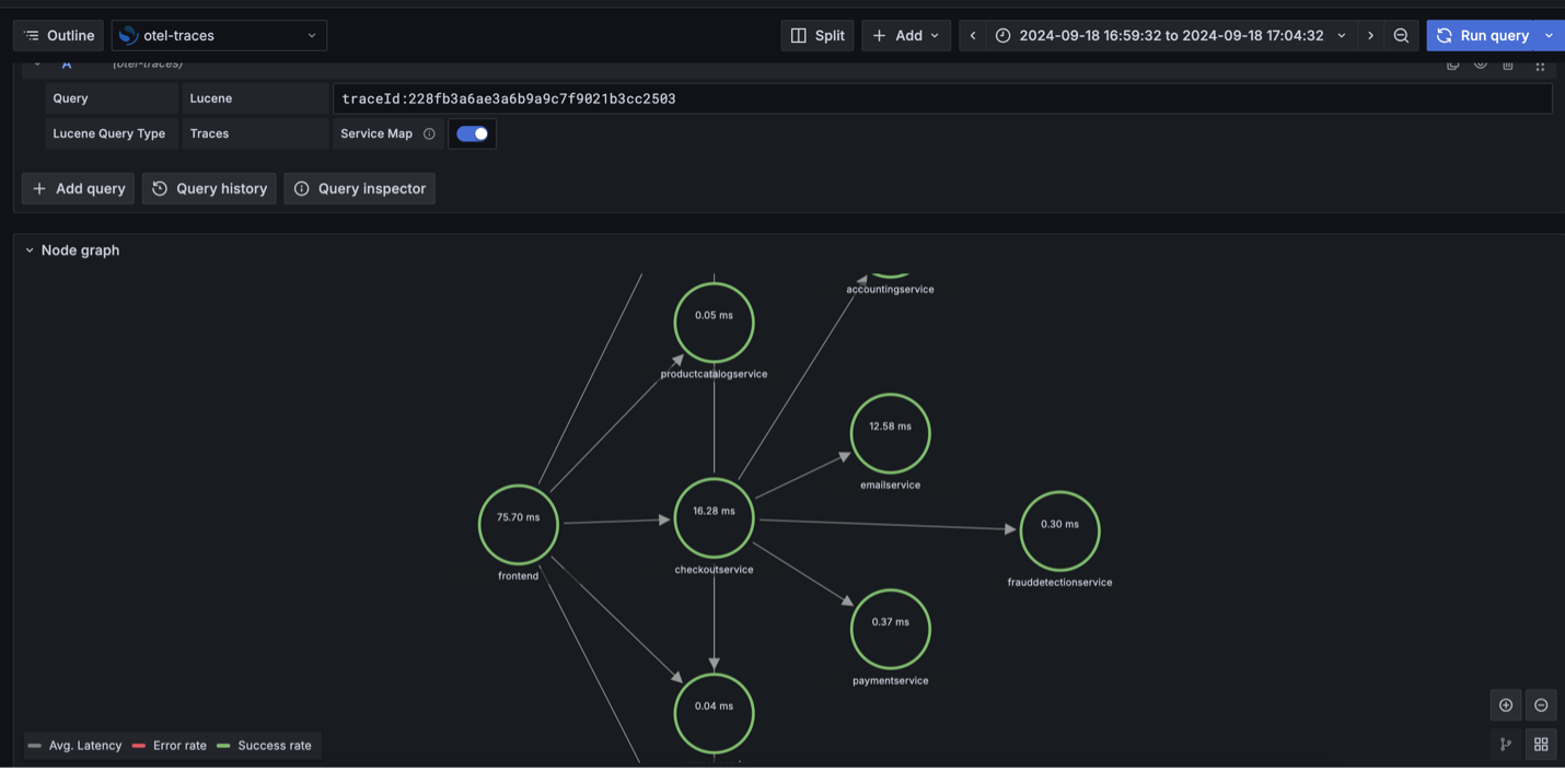
The following screenshot demonstrates the node graph visualization showing the correlation flow: instance metrics to logs to traces.

Clean up

Remove the infrastructure for this solution when not in use to avoid incurring unnecessary costs.

Conclusion

In this post, we showed how to use correlation as a helpful tool to gain insight into observability data stored in various stores.

Separating logs and traces into dedicated domains provides the following benefits:

  • Better resource allocation and scaling based on different workload patterns
  • Independent performance optimization for each data type
  • Simplified cost tracking and management
  • Enhanced security control with separate access policies

You can use this solution as a reference to build a scalable observability solution for your enterprise to detect, investigate, and remediate problems faster. This ability, when used along next-generation artificial intelligence and machine learning (AI/ML), helps to not only proactively react but predict and prevent problems before they occur. You can learn more about AI/ML with AWS.


About the Authors

Balaji Mohan is a Senior Delivery Consultant specializing in application and data modernization to the cloud. His business-first approach provides seamless transitions, aligning technology with organizational goals. Using cloud-centered architectures, he delivers scalable, agile, and cost-effective solutions, driving innovation and growth.

Senthil Ramasamy is a Senior Database Consultant at Amazon Web Services. He works with AWS customers to provide guidance and technical assistance on database services, helping them with database migrations to the AWS Cloud and improving the value of their solutions when using AWS.

Muthu Pitchaimani is a Search Specialist with Amazon OpenSearch Service. He builds large-scale search applications and solutions. Muthu is interested in the topics of networking and security, and is based out of Austin, Texas.

Accelerate operational analytics with Amazon Q Developer in Amazon OpenSearch Service

Post Syndicated from Esra Kayabali original https://aws.amazon.com/blogs/aws/accelerate-operational-analytics-with-amazon-q-developer-in-amazon-opensearch-service/

Today, I’m happy to announce Amazon Q Developer support for Amazon OpenSearch Service, providing AI-assisted capabilities to help you investigate and visualize operational data. Amazon Q Developer enhances the OpenSearch Service experience by reducing the learning curve for query languages, visualization tools, and alerting features. The new capabilities complement existing dashboards and visualizations by enabling natural language exploration and pattern detection. After incidents, you can rapidly create additional visualizations to strengthen your monitoring infrastructure. This enhanced workflow accelerates incident resolution and optimizes engineering resource usage, helping you focus more time on innovation rather than troubleshooting.

Amazon Q Developer in Amazon OpenSearch Service improves operational analytics by integrating natural language exploration and generative AI capabilities directly into OpenSearch workflows. During incident response, you can now quickly gain context on alerts and log data, leading to faster analysis and resolution times. When alert monitors trigger, Amazon Q Developer provides summaries and insights directly in the alerts interface, helping you understand the situation quickly without waiting for specialists or consulting documentation. From there, you can use Amazon Q Developer to explore the underlying data, build visualizations using natural language, and identify patterns to determine root causes. For example, you can create visualizations that break down errors by dimensions such as Region, data center, or endpoint. Additionally, Amazon Q Developer assists with dashboard configuration and recommends anomaly detectors for proactive alerting, improving both initial monitoring setup and troubleshooting efficiency.

Get started with Amazon Q Developer in OpenSearch Service
To get started, I go to my OpenSearch user interface and sign in. From the home page, I choose a workspace to test Amazon Q Developer in OpenSearch Service. For this demonstration, I use a preconfigured environment with the sample logs dataset available on the user interface.

This feature is on by default through the Amazon Q Developer Free tier, which is also on by default. You can disable the feature by unselecting the Enable natural language query generation checkbox under the Artificial Intelligence (AI) and Machine Learning (ML) section during domain creation or by editing the cluster configuration in console.

In OpenSearch Dashboards, I navigate to Discover from the left navigation pane. To use natural language to explore the data, I switch to PPL language in order to show the prompt box.

I choose the Amazon Q icon in the main navigation bar to open the Amazon Q panel. You can use this panel to create recommended anomaly detectors to drive alerting and use natural language to generate visualization.

I enter the following prompt in the Ask a natural language question text box:

Show me a breakdown of HTTP response codes for the last 24 hours

When results appear, Amazon Q automatically generates a summary of these results. You can control the summary display using the Show result summarization option under the Amazon Q panel to hide or show the summary. You can use the thumbs up or thumbs down buttons to provide feedback, and you can copy the summary to your clipboard using the copy button.

Other capabilities of Amazon Q Developer in OpenSearch Service are generating visualizations directly from natural language descriptions, providing conversational assistance for OpenSearch related queries, providing AI-generated summaries and insights for your OpenSearch alerts, and analyzing your data, and suggesting appropriate anomaly detectors.

Let’s look into how to generate visualizations directly from natural language descriptions. I choose Generate visualization from Amazon Q panel. I enter Create a bar chart showing the number of requests by HTTP status code in the input field and choose generate.

To refine the visualization, you can choose Edit visual and add style instructions such as Show me a pie chart or Use a light gray background with a white grid.

Now available
You can now use Amazon Q Developer in OpenSearch Service to reduce mean time to resolution, enable more self-service troubleshooting, and help teams extract greater value from your observability data.

The service is available today in US East (N. Virginia), US West (Oregon), Asia Pacific (Mumbai), Asia Pacific (Sydney), Asia Pacific (Tokyo), Canada (Central), Europe (Frankfurt), Europe (London), Europe (Paris), and South America (São Paulo) AWS Regions.

To learn more, visit the Amazon Q Developer documentation and start using Amazon Q Developer in your OpenSearch Service domain today.

— Esra


How is the News Blog doing? Take this 1 minute survey!

(This survey is hosted by an external company. AWS handles your information as described in the AWS Privacy Notice. AWS will own the data gathered via this survey and will not share the information collected with survey respondents.)

Introducing vector search with UltraWarm in Amazon OpenSearch Service

Post Syndicated from Kunal Kotwani original https://aws.amazon.com/blogs/big-data/introducing-vector-search-with-ultrawarm-in-amazon-opensearch-service/

Amazon OpenSearch Service has been providing vector database capabilities to enable efficient vector similarity searches using specialized k-nearest neighbor (k-NN) indexes to customers since 2019. This functionality has supported various use cases such as semantic search, Retrieval Augmented Generation (RAG) with large language models (LLMs), and rich media searching. With the explosion of AI capabilities and the increasing creation of generative AI applications, customers are seeking vector databases with rich feature sets.

OpenSearch Service also offers a multi-tiered storage solution to its customers in the form of UltraWarm and Cold tiers. UltraWarm provides cost-effective storage for less-active data with query capabilities, though with higher latency compared to hot storage. Cold tier offers even lower-cost archival storage for detached indexes that can be reattached when needed. Moving data to UltraWarm makes it immutable, which aligns well with use cases where data updates are infrequent like log analytics.

Until now, there was a limitation where UltraWarm or Cold storage tiers couldn’t store k-NN indexes. As customers adopt OpenSearch Service for vector use cases, we’ve observed that they’re facing high costs due to memory and storage becoming bottlenecks for their workloads.

To provide similar cost-saving economics for larger datasets, we are now supporting k-NN indexes in both UltraWarm and Cold tiers. This will enable you to save costs, especially for workloads where:

  • A significant portion of your vector data is accessed less frequently (for example, historical product catalogs, archived content embeddings, or older document repositories)
  • You need isolation between frequently and infrequently accessed workloads, minimizing the need to scale hot tier instances to help prevent interference from indexes that can be moved to the warm tier

In this post, we discuss this new capability and its use cases, and provide a cost-benefit analysis in different scenarios.

New capability: K-NN indexes in UltraWarm and Cold tiers

You can now enable UltraWarm and Cold tiers for your k-NN indexes from OpenSearch Service version 2.17 and up. This feature is available for both new and existing domains upgraded to version 2.17. K-NN indexes created after OpenSearch Service version 2.x are eligible for migration to warm and cold tiers. K-NN indexes using various types of engines (FAISS, NMSLib, and Lucene) are eligible to migrate.

Use cases

This multi-tiered approach to k-NN vector search benefits the following various use cases:

  • Long-term semantic search – Maintain searchability on years of historical text data for legal, research, or compliance purposes
  • Evolving AI models – Store embeddings from multiple versions of AI models, allowing comparisons and backward compatibility without the cost of keeping all data in hot storage
  • Large-scale image and video similarity – Build extensive libraries of visual content that can be searched efficiently, even as the dataset grows beyond the practical limits of hot storage
  • Ecommerce product recommendations – Store and search through vast product catalogs, moving less popular or seasonal items to cheaper tiers while maintaining search capabilities

Let’s explore real-world scenarios to illustrate the potential cost benefits of using k-NN indexes with UltraWarm and Cold storage tiers. We will be using us-east-1 as the representative AWS Region for these scenarios.

Scenario 1: Balancing hot and warm storage for mixed workloads

Let’s say you have 100 million vectors of 768 dimensions (around 330 GB of raw vectors) spread across 20 Lucene engine indexes of 5 million vectors each (roughly 16.5 GB), out of which 50% of data (about 10 indexes or 165 GB) is queried infrequently.

Domain setup without UltraWarm support

In this approach, you prioritize maximum performance by keeping all of the data in hot storage, providing the fastest possible query responses for the vectors. You deploy a cluster with 6x r6gd.4xlarge instances.

The monthly cost for this setup comes to $7,550 per month with a data instance cost of $6,700.

Although this provides top-tier performance for the queries, it might be over-provisioned given the mixed access patterns of your data.

Cost-saving strategy: UltraWarm domain setup

In this approach, you align your storage strategy with the observed access patterns, optimizing for both performance and cost. The hot tier continues to provide optimal performance for frequently accessed data, while less critical data moves to UltraWarm storage.

While UltraWarm queries experience higher latency compared to hot storage—this trade-off is often acceptable for less frequently accessed data. Additionally, since UltraWarm data becomes immutable, this strategy works best for stable datasets that don’t require any updates.

You keep the frequently accessed 50% of data (roughly 165 GB) in hot storage, allowing you to reduce your hot tier to 3x r6gd.4xlarge.search instances. For the less frequently accessed 50% of data (roughly 165 GB), you introduce 2x ultrawarm1.medium.search instances as UltraWarm nodes. This tier offers a cost-effective solution for data that doesn’t require the absolute fastest access times.

By tiering your data based on access patterns, you significantly reduce your hot tier footprint while introducing a small warm tier for less critical data. This strategy allows you to maintain high performance for frequent queries while optimizing costs for the entire system.

The hot tier continues to provide optimal performance for the majority of queries targeting frequently accessed data. For the warm tier, you see an increase in latency for queries on less frequently accessed data, but this is mitigated by effective caching on the UltraWarm nodes. Overall, the system maintains high availability and fault tolerance.

This balanced approach reduces your monthly cost to $5,350, with $3,350 for the hot tier and $350 for the warm tier, reducing the monthly costs by roughly 29% overall.

Scenario 2: Managing Growing Vector Database with Access-Based Patterns

Imagine your system processes and indexes vast amounts of content (text, images, and videos), generating vector embeddings using the Lucene engine for advanced content recommendation and similarity search. As your content library grows, you’ve observed clear access patterns where newer or popular content is queried frequently while older or less popular content sees decreased activity but still needs to be searchable.

To effectively leverage tiered storage in OpenSearch Service, consider organizing your data into separate indices based on expected query patterns. This index-level organization is important because data migration between tiers happens at the index level, allowing you to move specific indices to cost-effective storage tiers as their access patterns change.

Your current dataset consists of 150 GB of vector data, growing by 50 GB monthly as new content is added. The data access patterns show:

  • About 30% of your content receives 70% of the queries, typically newer or popular items
  • Another 30% sees moderate query volume
  • The remaining 40% is accessed infrequently but must remain searchable for completeness and occasional deep analysis

Given these characteristics, let’s explore a single-tiered and multi-tiered approach to managing this growing dataset efficiently.

Single-tiered configuration

For a single-tiered configuration, as the dataset expands, the vector data will grow to be around 400 GB over 6 months, all stored in a hot (default) tier. In the case of r6gd.8xlarge.search instances, the data instance count would be around 3 nodes.

The overall monthly costs for the domain under a single-tiered setup would be around $8050 with a data instance cost of around $6700.

Multi-tiered configuration

To optimize performance and cost, you implement a multi-tiered storage strategy using Index State Management (ISM) policies to automate the movement of indices between tiers as access patterns evolve:

  • Hot tier – Stores frequently accessed indices for fastest access
  • Warm tier – Houses moderately accessed indices with higher latency
  • Cold tier – Archives rarely accessed indices for cost-effective long-term retention

For the data distribution, you start with a total of 150 GB with a monthly growth of 50 GB. The following is the projected data distribution when the data reaches 400 GB at around the 6 month mark:

  • Hot tier – Approximately 100 GB (most frequently queried content) on 1x r6gd.8xlarge
  • Warm Tier – Approximately 100 GB (moderately accessed content) on 2x ultrawarm1.medium.search
  • Cold Tier – Approximately 200 GB (rarely accessed content)

Under the multi-tiered setup, the cost for the vector data domain totals $3880, including $2330 cost of data nodes, $350 cost of UltraWarm nodes, and $5.00 of cold storage costs.

You see compute savings as the hot tier instance size reduced by around 66%. Your overall cost savings were around 50% year-over-year with multi-tiered domains.

Scenario 3: Large-scale disk-based vector search with UltraWarm

Let’s consider a system managing 1 billion vectors of 768 dimensions distributed across 100 indexes of 10 million vectors each. The system predominantly uses disk-based vector search with 32x FAISS quantization for cost optimization, and about 70% of queries target 30% of the data, making it an ideal candidate for tiered storage.

Domain setup without UltraWarm support

In this approach, using disk-based vector search to handle the large-scale data, you deploy a cluster with 4x r6gd.4xlarge instances. This setup provides adequate storage capacity while optimizing memory usage through disk-based search.

The monthly cost for this setup comes to $6,500 per month with a data instance cost of $4,470.

Cost-saving strategy: UltraWarm domain setup

In this approach, you align your storage strategy with the observed query patterns, similar to Scenario 1.

You keep the frequently accessed 30% of data in hot storage, using 1x r6gd.4xlarge instances. For the less frequently accessed 70% of data, you use 2x ultrawarm1.medium.search instances.

You use disk-based vector search in both storage tiers to optimize memory usage. This balanced approach reduces your monthly cost to $3,270, with $1,120 for the hot tier and $400 for the warm tier, reducing the monthly costs by roughly 50% overall.

Get started with UltraWarm and Cold storage

To take advantage of k-NN indexes in UltraWarm and Cold tiers, make sure that your domain is running OpenSearch Service 2.17 or later. For instructions to migrate k-NN indexes across storage tiers, refer to UltraWarm storage for Amazon OpenSearch Service.

Consider the following best practices for multi-tiered vector search:

  • Analyze your query patterns to optimize data placement across tiers
  • Use Index State Management (ISM) to manage the data lifecycle across tiers transparently
  • Monitor cache hit rates using the k-NN stats and adjust tiering and node sizing as needed

Summary

The introduction of k-NN vector search capabilities in UltraWarm and Cold tiers for OpenSearch Service marks a significant step forward in providing cost-effective, scalable solutions for vector search workloads. This feature allows you to balance performance and cost by keeping frequently accessed data in hot storage for lowest latency, while moving less active data to UltraWarm for cost savings. While UltraWarm storage introduces some performance trade-offs and makes data immutable, these characteristics often align well with real-world access patterns where older data sees fewer queries and updates.

We encourage you to evaluate your current vector search workloads and consider how this multi-tier approach could benefit your use cases. As AI and machine learning continue to evolve, we remain committed to enhancing our services to meet your growing needs.

Stay tuned for future updates as we continue to innovate and expand the capabilities of vector search in OpenSearch Service.


About the Authors

Kunal Kotwani is a software engineer at Amazon Web Services, focusing on OpenSearch core and vector search technologies. His major contributions include developing storage optimization solutions for both local and remote storage systems that help customers run their search workloads more cost-effectively.

Navneet Verma is a senior software engineer at AWS OpenSearch . His primary interests include machine learning, search engines and improving search relevancy. Outside of work, he enjoys playing badminton.

Sorabh Hamirwasia is a senior software engineer at AWS working on the OpenSearch Project. His primary interest include building cost optimized and performant distributed systems.

Amazon OpenSearch Service vector database capabilities revisited

Post Syndicated from Jon Handler original https://aws.amazon.com/blogs/big-data/amazon-opensearch-service-vector-database-capabilities-revisited/

In 2023, we blogged about OpenSearch Service vector database capabilities. Since then, OpenSearch and Amazon OpenSearch Service have developed to bring better performance, lower cost, and enhanced tradeoffs. We’ve improved the OpenSearch Service hybrid lexical and semantic search methods using both dense vectors and sparse vectors. We’ve simplified connecting with and managing large language models (LLMs) hosted in other environments. We’ve brought native chunking and streamlined searching for chunked documents.

Where 2023 saw the explosion of LLMs for generative AI and LLM-generated vector embeddings for semantic search, 2024 was a year of consolidation and reification. Applications relying on Retrieval Augmented Generation (RAG) started to move from proof of concept (POC) to production, with all of the attendant concerns on hallucinations, inappropriate content, and cost. Builders of search applications began to move their semantic search workloads to production, seeking improved relevance to drive their businesses.

As we enter 2025, OpenSearch Service support for OpenSearch 2.17 brings these improvements to the service. In this post, we walk through 2024’s innovations with an eye to how you can adopt new features to lower your cost, reduce your latency, and improve the accuracy of your search results and generated text.

Using OpenSearch Service as a vector database

Amazon OpenSearch Service as a vector database provides you with the core capabilities to store vector embeddings from LLMs and use vector and lexical information to retrieve documents based on their lexical similarity, as well as their proximity in vector space. OpenSearch Service continues to support three vector engines: Facebook AI Similarity Search (FAISS), Non-Metric Space Library (NMSLIB), and Lucene. The service supports exact nearest-neighbor matching and approximate nearest-neighbor matching (ANN). For ANN, the service provides both Hierarchical Navigable Small World (HNSW), and Inverted File (IVF) for storage and retrieval. The service further supports a wealth of distance metrics, including Cartesian distance, cosine similarity, Manhattan distance, and more.

The move to hybrid search

The job of a search engine is to take as input a searcher’s intent, captured as words, locations, numeric ranges, dates, (and, with multimodal search, rich media such as images, videos, and audio) and return a set of results from its collection of indexed documents that meet the searcher’s need. For some queries, such as “plumbing fittings for CPVC pipes,” the words in a product’s description and the words that a searcher uses are sufficient to bring the right results, using the standard Term Frequency-Inverse Document Frequency (TF/IDF) similarity metric. These queries are characterized by a high level of specificity in the searcher’s intent, which matches well to the words they use and the product’s name and description. When the searcher’s intent is more abstract, such as “a cozy place to curl up by the fire,” the words are less likely to provide a good match.

To best serve their users across the range of queries, builders have largely started to take a hybrid search approach, using both lexical and semantic retrieval with combined ranking. OpenSearch provides a hybrid search that can blend lexical queries, k-Nearest Neighbor (k-NN) queries, and neural queries using OpenSearch’s neural search plugin. Builders can implement three levels of hybrid search—lexical filtering along with vectors, combining lexical and vector scores, and out-of-the-box score normalization and blending.

In 2024, OpenSearch improved its hybrid search capability with conditional scoring logic, improved constructs, removal of repetitive and unnecessary calculations, and optimized data structures, yielding as much as a fourfold latency improvement. OpenSearch also added support for parallelization of the query processing for hybrid search, which can deliver up to 25% improvement in latency. OpenSearch released post-filtering for hybrid queries, which can help further dial in search results. 2024 also saw the release of OpenSearch Service’s support for aggregations for hybrid queries.

Sparse vector search is a different way of combining lexical and semantic information. Sparse vectors reduce corpus terms to around 32,000 terms, the same as or closely aligned with the source. Sparse vectors use weights that are mostly zero or near-zero to provide a weighted set of tokens that capture the meaning of the terms. Queries are translated to the reduced token set, with generalization provided by sparse models. In 2024, OpenSearch introduced two-phase processing for sparse vectors that improves latency for query processing.

Focus on accuracy

One of builders’ primary concerns in moving their workloads to production has been balancing retrieval accuracy (derivatively, generated text accuracy) with the cost and latency of the solution. Over the course of 2024, OpenSearch and OpenSearch Service brought capabilities for trading off between cost, latency, and accuracy. One area of innovation for the service was to bring out various methods for reducing the amount of RAM consumed by vector embeddings through k-NN vector quantization methods. Beyond these new methods, OpenSearch has long supported product quantization for the FAISS engine. Product quantization uses training to build centroids for vector clusters on reduced-dimension sub-vectors and queries by matching these centroids. We’ve blogged about the latency and cost benefits of product quantization.

You use a chunking strategy to divide up long documents into smaller, retrievable pieces. The insight for doing that is that large pieces of text have many pools of meaning, captured in sentences, paragraphs, tables, and figures. You choose chunks that are units of meaning, within pools of related words. In 2024, OpenSearch made this process with a straightforward k-NN query, alleviating the need for custom processing logic. You can now represent long documents as multiple vectors in a nested field. When you run k-NN queries, each nested field is treated as a single vector (an encoded long document). Previously, you had to implement custom processing logic in your application to support the querying of documents represented as vector chunks. With this feature, you can run k-NN queries, making it seamless for you to create vector search applications.

Similarity search is designed around finding the k nearest vectors, representing the top-k most similar documents. In 2024, OpenSearch updated its k-NN query interface to include filtering k-NN results based on distance and vector score, alongside existing top-k support. This is ideal for use cases in which your goal is to retrieve all the results that are highly or sufficiently similar (for example, >= 0.95), minimizing the possibility of missing highly relevant results because they don’t meet a top-k threshold.

Reducing cost for production workloads

In 2024, OpenSearch introduced and extended scalar and binary quantization that reduce the number of bits used to store each vector. OpenSearch already supported product quantization for vectors. When using these scalar and byte quantization methods, OpenSearch reduces the number of bits used to store vectors in the k-NN index from 32-bit floating numbers down to as little as 1 bit per dimension. For scalar quantization, OpenSearch supports half precision (also called fp16), and quarter precision with 8-bit integers for two times and four times the compression, respectively.

For binary quantization, OpenSearch supports 1-bit, 2-bit, and 4-bit compression for 32, 16, and 8 times compression respectively. These quantization methods are lossy, reducing accuracy. In our testing, we’ve seen minimal impact on accuracy—as little as 2% on some standardized data sets—with up to 32 times reduction in RAM consumed.

In-memory handling of dense vectors drives cost in proportion to the number of vectors, the vector dimensions, and the parameters you set for indexing. In 2024, OpenSearch extended vector handling to include disk-based vector search. With disk-based search, OpenSearch keeps a reduced bit-count vector in memory for generating match candidates, retrieving full-precision vectors for the final scoring and ranking. The default compression of 32 times means a reduction in RAM needs by 32 times with an attendant reduction in the cost of the solution.

In 2024, OpenSearch introduced support for JDK21, which users can use to run OpenSearch clusters on the latest Java version. OpenSearch further enhanced performance by adding support for Single Instruction, Multiple Data (SIMD) instruction sets for exact search queries. Previous versions have supported SIMD for ANN search queries. The integration of SIMD for exact search requires no additional configuration steps, making it a seamless performance improvement. You can expect a significant reduction in query latencies and a more efficient and responsive search experience, with approximately 1.5 times faster performance than non-SIMD implementations.

Increasing innovation velocity

In November 2023, OpenSearch 2.9 was released on Amazon OpenSearch Service. The release included high-level vector database interfaces such as neural search, hybrid search, and AI connectors. For instance, users can use neural search to run semantic queries with text input instead of vectors. Using AI connectors to services such as Amazon SageMaker, Amazon Bedrock, and OpenAI, neural search encodes text into vectors using the customers’ preferred models and rewrites text-based queries into k-NN queries transparently. Effectively, neural search alleviated the need for customers to develop and manage custom middleware to perform this functionality, which is required by applications that use the k-NN APIs.

With the following 2.11 and 2.13 releases, OpenSearch added high-level interfaces for multimodal and conversational search, respectively. With multimodal search, customers can run semantic queries using a combination of text and image inputs to find images. As illustrated in this OpenSearch blog post, multimodal enables new search paradigms. An ecommerce customer, for instance, could use a photo of a shirt and describe alterations such as “with desert colors” to shop for clothes fashioned to their tastes. Facilitated by a connector to Amazon Bedrock Titan Multimodal Embeddings G1, vector generation and query rewrites are handled by OpenSearch.

Conversational search enabled yet another search paradigm, which users can use to discover information through chat. Conversational searches run RAG pipelines, which use connectors to generative LLMs such as Anthropic’s Claude 3.5 Sonnet in Amazon Bedrock, OpenAI ChatGPT, or DeepSeek R1 to generate conversational responses. A conversational memory module provides LLMs with persistent memory by retaining conversation history.

With OpenSearch 2.17, support for search AI use cases was expanded through AI-native pipelines. With ML inference processors (search request, response, ingestion), customers can enrich data flows on OpenSearch with any machine learning (ML) model or AI service. Previously, enrichments were limited to a few model types such as text embedding models to support neural search. Without limitations on model type support, the full breadth of search AI use cases can be powered by OpenSearch search and ingest pipeline APIs.

Conclusion

OpenSearch continues to explore and enhance its features to build scalable, cost-effective, and low-latency semantic search and vector database solutions. The OpenSearch Service neural plugin, connector framework, and high-level APIs reduce complexity for builders, making the OpenSearch Service vector database more approachable and powerful. 2024’s improvements span text-based exact searches, semantic search, and hybrid search. These performance enhancements, feature innovations, and integrations provide a robust foundation for creating AI-driven solutions that provide better performance and more accurate results. Try out these new features with the latest version of OpenSearch.


About the Author

Jon Handler is Director of Solutions Architecture for Search Services at Amazon Web Services, based in Palo Alto, CA. Jon works closely with OpenSearch and Amazon OpenSearch Service, providing help and guidance to a broad range of customers who have generative AI, search, and log analytics workloads for OpenSearch. Prior to joining AWS, Jon’s career as a software developer included four years of coding a large-scale, eCommerce search engine. Jon holds a Bachelor of the Arts from the University of Pennsylvania, and a Master of Science and a Ph. D. in Computer Science and Artificial Intelligence from Northwestern University.

Amazon Prime Video advances search for sports using Amazon OpenSearch Service

Post Syndicated from Radhika Chandak original https://aws.amazon.com/blogs/big-data/amazon-prime-video-advances-search-for-sports-using-amazon-opensearch-service/

Passionate sports viewers expect to easily discover and access sports events and their favorite teams, leagues, and players. Providing a robust and intuitive search experience is crucial for the success of Prime Video Sports. With a vast, rapidly growing catalog of live and on-demand sports offerings, a well-designed search architecture allows Prime Video Sports to cater to this engaged audience, streamlining navigation and reducing friction in the user experience. The Prime Video search experience is one of the most clicked on elements in the global navigation bar. Search enables highly relevant recommendations and drives increased viewership and engagement. By prioritizing a seamless search experience that caters to the needs of sports fans, Prime Video has enhanced the overall customer experience, fostering trust and loyalty that contributes to the platform’s long-term growth and success. In this post, we will walk you through how Prime Video used Amazon OpenSearch Service and its AI and machine learning (AI/ML) capabilities to build a more intuitive and enhanced sports search experience.

Challenges

The Prime Video search experience was originally designed to help customers discover trending movies and TV shows that carry durable stats including ratings, viewership, and so on. As Prime Video began to acquire sports rights, they needed to rethink the approach, which was focused primarily on TV shows and movies, to understand the customers’ intent and surface the right content. The approach for TV shows and movies didn’t work as well for live sports because of the more temporal and seasonal nature of sports content making every title a cold start. For example, a search for “soccer live” surfaced documentaries such as “This is football: Season 1” and “Ronaldo VS Messi – Face Off!” rather than live soccer matches. While those entertainment options are perfectly fine on their own, they didn’t fulfill the customers’ goal of finding and watching live or upcoming games for their favorite sports. This disconnect between search queries and relevant results created challenges for customers trying to access the sports content they wanted. By surfacing these relevant sports events in search results, Prime Video enhanced the customer experience, helping customers discover the full breadth of sports coverage available on Prime Video and finding their favorite sports events. To address these issues and better serve the needs of sports fans, in 2024, Prime Video enhanced its sports-specific search capabilities, incorporating deeper sports understanding and using state-of-the-art search techniques, creating an improved and intelligent search system.

Solution overview

In 2024, Prime Video Sports Search delivered the first version of an enhanced sports search functionality powering the experience through a two layer solution comprised of coarse retrieval using semantic search and binary search relevance classification. Semantic search is a technique of searching for information that goes beyond just matching keywords. It matches queries to data (sports events in this case) based on vector embeddings, which capture the meaning of words, phrases, and sentences. The vectors can have n dimensions; when mapped into an n-dimensional space, data that is close in semantic meaning (not a direct text match) will be close to each other in the space, as shown in the following diagram of a two-dimensional vector space of sports matches (in yellow) and search queries (in green).

The foundation of using vector search for sports is the creation of vector embeddings for each sport event present in the Prime Video Sports Catalog. As event data is ingested, textual information including title, sports, team names, leagues, and other event details are used to generate a unique vector representation for each sports event. This allows the system to capture the semantic meaning and relationships between different events—including abbreviations, nicknames, and so on—that are often used by customers to search. When a customer searches for something related to sports, their query is also converted into a vector. The system then performs a K-nearest neighbor (KNN) search, comparing the customer’s query vector to the vectors of all sports events in the catalog. The events with vectors that are closest to the query vector are identified as the most relevant matches, even if the searched words were not directly indexed. For example, Thursday Night Football events might be indexed without the abbreviation tnf, however these games will be returned by semantic search if a customer searches using “tnf” as their search query.

The following figure shows a high level indexing and query flow for a KNN vector search.


Finding the nearest vectors isn’t enough—the system also runs each of these potentially relevant events through a custom binary relevance classification machine learning (ML) model, trained in-house. This allows the system to filter out any events that might be only tangentially related to the original search, leaving behind a refined list of the most pertinent and relevant results for the customer.

Finally, these highly relevant events are ranked and surfaced to the customer with factors like the event’s current live status and upcoming schedule playing a key role in determining the optimal order to display the results. This combined use of vector semantic search and relevance classification enables Prime Video to provide customers with a sports search experience that accurately surfaces the content they’re looking for, significantly enhancing their ability to discover and access the live, upcoming, and recently ended games that they’re most interested in.

Procedure

The vector semantic search implementation we developed consists of two main components: a KNN search index and an endpoint to invoke the text embedding model. To host these components, we used AWS services—the custom text embedding model was deployed on Amazon SageMaker, while the KNN index was created using OpenSearch Service, and hosted on a managed cluster consisting of more than 50 data nodes.

Both of these components are designed to handle real-time customer traffic at a scale of thousands of requests per second. We simplified our system’s application layer by using ready-to-use solutions available in AWS. The Amazon OpenSearch Ingestion pipeline enabled a seamless, code-free integration, allowing us to write sports data from an Amazon DynamoDB table directly into the OpenSearch Service index, eliminating the need for traditional extract, transform, and load (ETL) processes. Furthermore, we used the Neural Search feature of OpenSearch Service instead of directly integrating our application layer with SageMaker for text-to-vector conversion. This approach enables internal text-to-vector transformation, facilitating vector search during both ingestion and search phases. The Neural Search plugin of OpenSearch Service directly communicates with a text embedding model deployed on SageMaker as a real-time inference endpoint using ML connectors.

This architecture—illustrated in the following figure—enabled us to build a scalable and efficient vector search solution, taking advantage of the strengths of various AWS services to simplify the implementation and improve performance.

OpenSearch Ingestion : No-ETL data transfer from DynamoDB to an OpenSearch Service index

Before indexing the sports data in OpenSearch Service, the data is first stored in a DynamoDB table. This layer of storage allows us to maintain a database of all sports events and their metadata required to enable search. This layer acts as a source of truth for sports data that isn’t impacted by the evolution of customer use cases and their respective implementation.

To seamlessly transfer this data from DynamoDB to the OpenSearch Service index, we used an OpenSearch Ingestion pipeline. This allowed us to set up real-time data transfer with a zero ETL integration, abstracting away the data indexing from the application layer. The OpenSearch Ingestion pipeline configuration enables us to specify a schema mapping between the DynamoDB table and the expected document schema in OpenSearch Service. This configuration also allows us to perform data formatting operations on specific fields and configure a dead-letter queue (DLQ) if needed. The steps to setup an OpenSearch Ingestion pipeline can be found in this blog post.

Embedding model setup on SageMaker

At the core of our vector search implementation is the text-embedding model, which plays a crucial role in capturing the semantic meaning of sports-related data. The Sports Search Science team developed this text-embedding model and deployed it on SageMaker as a real-time inference endpoint using AWS Cloud Development Kit (AWS CDK).

The process of creating the SageMaker endpoint requires two key artifacts:

With these two components in place, we used the AWS CDK to programmatically provision the SageMaker endpoint, ensuring a seamless and consistent deployment of the text-embedding model. By using the capabilities of AWS services, such as SageMaker, Amazon ECR, and Amazon S3, we were able to build a scalable and efficient text-embedding model infrastructure to power the vector search solution.

ML connectors

To facilitate access to machine learning models hosted on platforms, such as SageMaker or Amazon Bedrock, OpenSearch Service provides ML connectors. These connectors enable direct integration between OpenSearch Service and external machine learning models.

In our case, the ML connector allows OpenSearch Service to directly invoke the SageMaker endpoint where our custom text-embedding model is deployed. This built-in integration between OpenSearch Service and the SageMaker hosted model simplifies the overall architecture and eliminates the need for the application layer to manage the communication between these two components.

By using the ML connectors provided by the OpenSearch Service ML plugin, we were able to seamlessly integrate our text-embedding model—which is hosted on SageMaker—into the OpenSearch-powered vector search solution. This integration streamlines the data ingestion and querying pipeline making the implementation simpler and more intuitive.

Neural search

To simplify the application layer of our vector search solution, we used the Neural Search capabilities provided by OpenSearch Service. This feature allows us to send only the text data to the index, without the need to explicitly manage the vector embedding generation and indexing. Using neural search helped simplify the application layer of the system by abstracting the generations and management of vectors required to perform a KNN search. During ingestion, neural search transforms document text into vector embeddings and indexes both the text and its vector embeddings in a vector index. When you use a neural query during search, neural search converts the query text into vector embeddings, uses vector search to compare the query and sports event embeddings, and returns the closest results. This abstracts away the need to integrate with SageMaker in the application layer to generate vector embeddings during ingestion and search.

The process of setting up a neural search index with a SageMaker-hosted inference endpoint involves the following detailed steps:

  1. Create an ML connector and register your model in OpenSearch Service: This step generates a model ID that you’ll need in the subsequent neural index setup.
  2. Create a neural ingest pipeline: An ingest pipeline is a sequence of processors that are applied to documents as they’re ingested into an index. To enable neural search, you can define the text_embedding processor in the pipeline. This processor converts the text in a document field to vector embeddings, and the field_map configuration determines the input and output fields for this process.
  3. Create the neural search index: To use the text embedding processor defined in the ingest pipeline, you can create a KNN index and specify the pipeline created in the previous step as the default pipeline.
  4. Run a neural query: To verify your neural search setup, run a neural query by providing a search text and evaluate the results.

By following these steps, you can set up a neural search index in OpenSearch Service and run a neural query. The neural query can perform KNN vector search internally, while only requiring the input of text data during both indexing and querying. This simplifies the application layer and uses the built-in vector embedding generation and indexing capabilities provided by the OpenSearch Service Neural Search feature.

Outcomes

The initial launch of this architecture for sports search had a measurably positive impact on customer experience. We observed a statistically significant increase in search-attributed conversions including streams, purchases, subscriptions, and so on. Offline analysis of the results delivered to customers indicated an improvement in the precision of search results and a reduction in the irrelevance rate of the content shown.

Additionally, we saw that customers engaged with the search feature more frequently, as it was now surfacing results that much more closely aligned with what they were looking for. This increased engagement led to greater discovery of relevant titles on the Prime Video service, including titles that had received little engagement prior to the changes.

Overall, the data clearly demonstrated that by tailoring the specific needs of sports fans into the search experience, we significantly improved their ability to find and access desired content. By developing a smarter search system that better understands sports intent, we have driven more meaningful customer activity and increased conversions directly from search interactions.

Conclusion

By using the innovative AI/ML capabilities of Amazon OpenSearch Service, Prime Video was able to create a cutting-edge search experience that effectively addressed the unique challenges presented by highly dynamic, high-volume sports content. In addition, by overcoming the hurdles that come with such large scale, Prime Video Sports Search was able to contribute valuable improvements and enhancements back to the OpenSearch open source community. These contributions help to pave the way for other developers to more readily use the advanced AI/ML features that OpenSearch Service offers.

This collaboration between Prime Video Sports Search and OpenSearch Service has resulted in a best-in-class search capability that can seamlessly accommodate the unique requirements of live sports content. It’s a partnership that has allowed the products to grow and innovate in tandem, to the benefit of customers seeking exceptional search and discovery experiences.

If you want to build a search experience that understands user intent beyond keyword matching, try the semantic search algorithm with OpenSearch Service and its AI/ML capabilities. If you have any questions, leave a comment below.


About the authors

Radhika Chandak is a Software Development Engineer at Amazon Prime Video, where she has been working for the past 3 years. Her focus is on creating high-velocity customer experiences, with a particular emphasis on building state-of-the-art search experiences for sports content. Radhika is passionate about developing solutions that solve customer problems and delight users. Her expertise lies in crafting innovative approaches to enhance the Prime Video Sports platform, ensuring seamless and engaging experiences for sports enthusiasts.

Anna Chalupowicz is a Software Development Manager at Amazon Prime Video Sports, with 6 years of diverse experience within Amazon. For the last 3.5 years, Anna has been working in Prime Video Sports, where she focuses on developing high-scale solutions and architectural approaches that directly benefit customers. With a passion for collaborative learning and knowledge sharing, Anna finds joy in tackling complex technical challenges and using data-driven insights to enhance the customer experience.

Yaliang Wu is a Software Engineering Manager at AWS, focusing on OpenSearch projects, machine learning, and generative AI applications.

Supercharge your RAG applications with Amazon OpenSearch Service and Aryn DocParse

Post Syndicated from Jon Handler original https://aws.amazon.com/blogs/big-data/supercharge-your-rag-applications-with-amazon-opensearch-service-and-aryn-docparse/

The old adage “garbage in, garbage out” applies to all search systems. Whether you are building for ecommerce, document retrieval, or Retrieval Augmented Generation (RAG), the quality of your search results depends on the quality of your search documents. Downstream, RAG systems improve the quality of generated answers by adding relevant data from other systems to the generative prompt. Most RAG solutions use a search engine to search for this relevant data. To get great responses, you need great search results, and to get great search results, you need great data. If you don’t properly partition, extract, enrich, and clean your data before loading it, your search results will reflect the poor quality of your search documents.

Aryn DocParse segments and labels PDF documents, runs OCR, extracts tables and images, and more. It turns your messy documents into beautiful, structured JSON, which is the first step of document extract, transform, and load (ETL). DocParse runs the open source Aryn Partitioner and its state-of-the-art, open source deep learning DETR AI model trained on over 80,000 enterprise documents. This leads to up to 6 times more accurate data chunking and 2 times improved recall on vector search or RAG when compared to off-the-shelf systems. The following screenshot is an example of how DocParse would segment a page in an ETL pipeline. You can visualize labeled bounding boxes for each document segment using the Aryn Playground.

In this post, we demonstrate how to use Amazon OpenSearch Service with purpose-built document ETL tools, Aryn DocParse and Sycamore, to quickly build a RAG application that relies on complex documents. We use over 75 PDF reports from the National Transportation Safety Board (NTSB) about aircraft incidents. You can refer to the following example document from the collection. As you can see, these documents are complex, containing tables, images, section headings, and complicated layouts.

Let’s get started!

Prerequisites

Complete the following prerequisite steps:

  1. Create an OpenSearch Service domain. For more details, see Creating and managing Amazon OpenSearch Service domains. You can create a domain using the AWS Management Console, AWS Command Line Interface (AWS CLI), or SDK. Be sure to choose public access for your domain, and set up a user name and password for your domain’s primary user so that you can run the notebook from your laptop, Amazon SageMaker Studio, or an Amazon Elastic Compute Cloud (EC2) instance. To keep costs low, you can create an OpenSearch Service domain with a single t3.small search node in a dev/test configuration for this example. Take note of the domain’s endpoint to use in later steps.
  2. Get an Aryn API key.
  3. You will be using Anthropic’s Claude large language model (LLM) on Amazon Bedrock in the ETL pipeline, so make sure your notebook has access to AWS credentials with the required permissions.
  4. Have access to a Jupyter environment to open and run the notebook.

Use DocParse and Sycamore to chunk data and load OpenSearch Service

Although you can generate an ETL pipeline to load your OpenSearch Service domain using the Aryn DocPrep UI, we will instead focus on the underlying Sycamore document ETL library and write a pipeline from scratch.

Sycamore was designed to make it straightforward for developers and data engineers to define complex data transformations over large collections of documents. Borrowing some ideas from popular dataflow frameworks like Apache Spark, Sycamore has a core abstraction called the DocSet. Each DocSet represents a collection of unstructured documents, and is scalable from a single document to many thousands. Each document in a DocSet has an arbitrary set of key-value properties as metadata, as well as an ordered list of elements. An Element corresponds to a chunk of the document that can be processed and embedded separately, such as a table, headline, text passage, or image. Like documents, Elements can also contain arbitrary key-value properties to encode domain- or application-specific metadata.

Notebook walkthrough

We’ve created a Jupyter notebook that uses Sycamore to orchestrate data preparation and loading. This notebook uses Sycamore to create a data processing pipeline that sends documents to DocParse for initial document segmentation and data extraction, then runs entity extraction and data transforms, and finally loads data into OpenSearch Service using a connector.

Copy the notebook into your Amazon SageMaker JupyterLab space, launch it using a Python kernel, then walk through the cells along with the following procedures.

To install Sycamore with the OpenSearch Service connector and local inference features necessary to create vector embeddings, run the first cell of the notebook:

!pip install 'sycamore-ai[opensearch,local-inference]'

In the second cell of the notebook, fill in your ARYN_API_KEY. You should be able to complete the example in the notebook for less than $1.

Cell 3 does the initial work of reading the source data and preparing a DocSet for that data. After initializing the Sycamore context and setting paths, this code calls out to DocParse to create a partitioned_docset:

partitioned_docset = (
  docset.partition(
    partitioner=ArynPartitioner(
      extract_table_structure=True,
      extract_images=True
    )
  ).materialize(
      path="./opensearch-tutorial/partitioned-docset",
      source_mode=sycamore.MATERIALIZE_USE_STORED
    )
)
partitioned_docset.execute()

The previous code uses materialize to create and save a checkpoint. In future runs, the code will use the materialized view to save a few minutes of time. partitioned_docset.execute() forces the pipeline to execute. Sycamore uses lazy execution to create efficient query plans, and would otherwise execute the pipeline at a much later step.

After this step, each document in the DocSet now includes the partitioned output from DocParse, including bounding boxes, text content, and images from that document, stored as elements.

Entity extraction

Part of the key to building good retrieval for RAG is adding structured information that enables accurate filtering for the search query. Sycamore provides LLM-powered transforms that can extract this information and store it as structured properties, enriching the document. Sycamore can do unsupervised or supervised schema extraction, where it pulls out fields based on a JSON schema you provide. When executing these types of transforms, Sycamore will take a specified number of elements from each document, use an LLM to extract the specified fields, and include them as properties in the document.

Cell 4 uses supervised schema extraction, setting the schema as the fields you want to extract. You can add additional information that is passed to the LLM performing the entity extraction. The location property is an example of this:

schema = {
            'type': 'object',
            'properties': {'accidentNumber': {'type': 'string'},
                           'dateAndTime': {'type': 'date'},
                           'location': {
                             'type': 'string', 
                             'description': 'US State where the incident occured'
                           },
                           'aircraft': {'type': 'string'},
                           'aircraftDamage': {'type': 'string'},
                           'injuries': {'type': 'string'},
                           'definingEvent': {'type': 'string'}},
            'required': ['accidentNumber',
                         'dateAndTime',
                         'location',
                         'aircraft']
    }

schema_name = 'FlightAccidentReport'
property_extractor=LLMPropertyExtractor(llm=llm, num_of_elements=20, schema_name=schema_name, schema=schema)

The LLMPropertyExtractor uses the schema you provided to add additional properties to the document. Next, summarize the images to add additional information to improve retrieval.

Image summarization

There’s more information in your documents than just text—as the saying goes, a picture is worth 1,000 words! When your documents contain images, you can capture the information in those images using Sycamore’s SummarizeImages transform. SummarizeImages uses an LLM to compute a text summary for the image, then adds the summary to that element. Sycamore will also send related information about the image, like a caption, to the LLM to aid with summarization. The following code (in cell 4) takes advantage of DocParse type labeling to automatically apply SummarizeImages to image elements:

enriched_docset = enriched_docset.transform(SummarizeImages, summarizer=LLMImageSummarizer(llm=llm))

This cell can take up to 20 minutes to complete.

Now that your image elements contain additional retrieval information, it’s time to clean and normalize the text in the elements and extracted entities.

Data cleaning and formatting

Unless you are in direct control of the creation of the documents you are processing, you will likely need to normalize that data and make it ready for search. Sycamore makes it straightforward for you to clean messy data and bring it to a regular form, fixing data quality issues.

For example, in the NTSB data, dates in the incident report are not all formatted the same way, and some US state names are shown as abbreviations. Sycamore makes it straightforward to write custom transformations in Python, and also provides several useful cleaning and formatting transforms. Cell 4 uses two functions in Sycamore to format the state names and dates:

formatted_docset = (
  enriched_docset
  
  # Converts state abbreviations to their full names.
  .map(lambda doc: USStateStandardizer.standardize(
    doc, key_path = ["properties","entity","location"])
  )

  # Converts datetime into a common format
  .map(lambda doc: DateTimeStandardizer.standardize(
    doc, key_path = ["properties","entity","dateTime"])
  )
)

The elements are now in normal form, with extracted entities and image descriptions. The next step is to merge together semantically related elements to create chunks.

Create final chunks and vector embeddings

When you prepare for RAG, you create chunks—parts of the full document that are related information. You design your chunks so that as a search result they can be added to the prompt to provide a unit of meaning and information. There are many ways to approach chunking. If you have small documents, sometimes the whole document is a chunk. If you have larger documents, sentences, paragraphs, or even sections can be a chunk. As you iterate on your end application, it’s common to adjust the chunking strategy to fine-tune the accuracy of retrieval. Sycamore automates the process of building chunks by merging together the elements of the DocSet.

At this stage of the processing in cell 4, each document in our DocSet has a set of elements. The following code merges elements together using a chunking strategy to create larger elements that will improve query results. For instance, the DocSet might have an element that is a table and an element that is a caption for that table. Merging those elements together creates a chunk that’s a better search result.

We will use Sycamore’s Merge transform with the GreedySectionMerger merging strategy to add elements in the same document section together into larger chunks:

merger = GreedySectionMerger(
  tokenizer=HuggingFaceTokenizer(
    "sentence-transformers/all-MiniLM-L6-v2"),
  max_tokens=512
)
chunked_docset = formatted_docset.merge(merger=merger)

With chunks created, it’s time to add vector embeddings for the chunks.

Create vector embeddings

Use vector embeddings to enable semantic search in OpenSearch Service. With semantic search, retrieve documents that are close to a query in a multidimensional space, rather than by matching words exactly. In RAG systems, it’s common to use semantic search along with lexical search for a hybrid search. Using hybrid search, you get best-of-all-worlds retrieval.

The code in cell 4 creates vector embeddings for each chunk. You can use a variety of different AI models with Sycamore’s embed transform to create vector embeddings. You can run these locally or use a service like Amazon Bedrock or OpenAI. The embedding model you choose has a huge impact on your search quality, and it’s common to experiment with this variable as well. In this example, you create embeddings locally using a model called GTE:

model_name = "thenlper/gte-small"
embedded_docset = chunked_docset.spread_properties(["entity", "path"]).explode().embed(
      embedder=SentenceTransformerEmbedder(batch_size=10_000, model_name=model_name)
)
embedded_docset = embedded_docset.materialize(
  path="./opensearch-tutorial/embedded-docset",
  source_mode=sycamore.MATERIALIZE_USE_STORED
)
embedded_docset.execute()

You use materialize again here, so you can checkpoint the processed DocSet before loading. If there is an error when loading the indexes, you can retry without running the last few steps of the pipeline again.

Load OpenSearch Service

The final ETL step is loading the prepared data into OpenSearch Service vector and keyword indexes to power hybrid search for the RAG application. Sycamore makes loading indexes straightforward with its set of connectors. Cell 5 adds configuration, specifying the OpenSearch Service domain endpoint and what indexes to create. If you’re following along, be sure to replace YOUR-DOMAIN-ENDPOINT, YOUR-OPENSEARCH-USERNAME, and YOUR-OPENSEARCH-PASSWORD in cell 5 with the actual values.

If you copied your domain endpoint from the console, it will start with the https:// URL scheme. When you replace YOUR-DOMAIN-ENDPOINT, be sure to remove https://.

In cell 6, Sycamore’s OpenSearch connector loads the data into an OpenSearch index:

embedded_docset.write.opensearch(
    os_client_args=openSearch_client_args,
    index_name="aryn-rag-demo",
    index_settings=index_settings,
)

Congratulations! You’ve completed some of the core processing steps to take raw PDFs and prepare them as a source for retrieval in a RAG application. In the next cells, you will run a couple of RAG queries.

Run a RAG query on OpenSearch using Sycamore

In cell 7, Sycamore’s query and summarize functions create a RAG pipeline on the data. The query step uses OpenSearch’s vector search to retrieve the relevant passages for RAG. Then, cell 8 runs a second RAG query that filters on metadata that Sycamore extracted in the ETL pipeline, yielding even better results. You could also use an OpenSearch hybrid search pipeline to perform hybrid vector and lexical retrieval.

Cell 7 asks “What was common with incidents in Texas, and how does that differ from incidents in California?” Sycamore’s summarize_data transform runs the RAG query, and uses the LLM specified for generation (in this case, it’s Anthropic’s Claude):

Based on the provided data, it appears that the common factor among the incidents 
in Texas was that many of them involved substantial aircraft damage, with some resulting 
in injuries or fatalities. The incidents covered a range of aircraft types, including small
planes like Cessnas and Pipers, as well as a helicopter. The defining events varied, 
including loss of control on the ground, engine failures, fuel issues, and collisions 
with terrain or objects.

In contrast, the incidents in California seemed to primarily involve substantial aircraft
damage as well, but with fewer injuries reported. The defining events included loss of 
control on the ground, collisions during takeoff or landing, and a miscellaneous/other event.
One key difference is that the Texas incidents included a fatal accident (CEN23FA084) 
involving a Piper PA46 that resulted in 4 fatalities and 1 serious injury after impacting 
terrain. The California incidents did not appear to have any fatal accidents based on the 
provided data.

Additionally, while both states had incidents involving loss of control on the ground, the 
Texas incidents seemed to have a higher proportion of engine failures, fuel issues, and 
collisions with terrain or objects as defining events compared to California.

Overall, while both states experienced aviation incidents resulting in substantial aircraft
damage, the Texas incidents tended to be more severe in terms of injuries and fatalities, 
with a higher prevalence of engine failures, fuel issues, and terrain/object collisions as 
contributing factors.

Using metadata filters in a RAG query

Cell 8 makes a small adjustment to the code to add a filter to the vector search, filtering for documents from incidents with the location of California. Filters increase the accuracy of chatbot responses by removing irrelevant data from the result the RAG pipeline passes to the LLM in the prompt.

To add a filter, cell 8 adds a filter clause to the k-nearest neighbors (k-NN) query:

os_query["query"]["knn"]["embedding"]["filter"] = {"match_phrase": {"properties.entity.location": "California"}}

The output from the RAG query is as follows:

Based on the database entries provided, several incidents occurred in California during January 2023:

1. On January 12th, a Cessna 180K aircraft sustained substantial damage in a collision during takeoff 
or landing at Agua Caliente Springs, California. There was 1 person on board with no injuries reported.

2. On January 20th, a Cessna 195A aircraft sustained substantial damage due to a los of control on the 
ground at Calexico, California. There were 3 people on board with no injuries.  

3. On January 15th, a Piper PA-28-180 aircraft sustained substantial damage in a miscellaneous incident 
at San Diego, California during an instructional flight. There were 4 people on board with no injuries.

4. On January 1st, a Cessna 172 aircraft sustained substantial damage in a collision during takeoff or 
landing at Watsonville, California during an instructional flight. There was 1 serious injury reported.

5. On January 27th, a Cessna T210N aircraft sustained substantial damage when it descended into a ravine 
and impacted the ground about 2,000 feet short of the runway threshold at Murrieta, California. There were
1 serious injury and 1 minor injury reported. The engine did not respond during the landing approach.

The details provided in the database entries, such as aircraft type, location, date/time, damage level, 
injuries, and a brief description of the defining event, serve as evidence for these incidents occurring 
in California during the specified time period.

Clean up

Be sure to clean up the resources you deployed for this walkthrough:

  1. Delete your OpenSearch Service domain.
  2. Remove any Jupyter environments you created.

Conclusion

In this post, you used Aryn DocParse and Sycamore to parse, extract, enrich, clean, embed, and load data into vector and keyword indexes in OpenSearch Service. You then used Sycamore to run RAG queries on this data. Your second RAG query used an OpenSearch filter on metadata to get a more accurate result.

The way in which your documents are parsed, enriched, and processed has a significant impact on the quality of your RAG queries. You can use the examples in this post to build your own RAG systems with Aryn and OpenSearch Service, and iterate on the processing and retrieval strategies as you build your generative AI application.


About the Authors

Jon Handler is Director of Solutions Architecture for Search Services at Amazon Web Services, based in Palo Alto, CA. Jon works closely with OpenSearch and Amazon OpenSearch Service, providing help and guidance to a broad range of customers who have search and log analytics workloads for OpenSearch. Prior to joining AWS, Jon’s career as a software developer included four years of coding a large-scale ecommerce search engine. Jon holds a Bachelor of the Arts from the University of Pennsylvania, and a Master’s of Science and a PhD in Computer Science and Artificial Intelligence from Northwestern University.

Jon is the founding Chief Product Officer at Aryn. Prior to that, he was the SVP of Product Management at Dremio, a data lake company. Earlier, Jon was a Director at AWS, and led product management for in-memory database services (Amazon ElastiCache and Amazon MemoryDB for Redis), Amazon EMR (Apache Spark and Hadoop), and founded and was GM of the blockchain division. Jon has an MBA from Stanford Graduate School of Business and a BA in Chemistry from Washington University in St. Louis.

Improve search results for AI using Amazon OpenSearch Service as a vector database with Amazon Bedrock

Post Syndicated from Jon Handler original https://aws.amazon.com/blogs/big-data/improve-search-results-for-ai-using-amazon-opensearch-service-as-a-vector-database-with-amazon-bedrock/

Artificial intelligence (AI) has transformed how humans interact with information in two major ways—search applications and generative AI. Search applications include ecommerce websites, document repository search, customer support call centers, customer relationship management, matchmaking for gaming, and application search. Generative AI use cases include chatbots with Retrieval-Augmented Generation (RAG), intelligent log analysis, code generation, document summarization, and AI assistants. AWS recommends Amazon OpenSearch Service as a vector database for Amazon Bedrock as the building blocks to power your solution for these workloads.

In this post, you’ll learn how to use OpenSearch Service and Amazon Bedrock to build AI-powered search and generative AI applications. You’ll learn about how AI-powered search systems employ foundation models (FMs) to capture and search context and meaning across text, images, audio, and video, delivering more accurate results to users. You’ll learn how generative AI systems use these search results to create original responses to questions, supporting interactive conversations between humans and machines.

The post addresses common questions such as:

  1. What is a vector database and how does it support generative AI applications?
  2. Why is Amazon OpenSearch Service recommended as a vector database for Amazon Bedrock?
  3. How do vector databases help prevent AI hallucinations?
  4. How can vector databases improve recommendation systems?
  5. What are the scaling capabilities of OpenSearch as a vector database?

How vector databases work in the AI workflow

When you’re building for search, FMs and other AI models convert various types of data (text, images, audio, and video) into mathematical representations called vectors. When you use vectors for search, you encode your data as vectors and store those vectors in a vector database. You further convert your query into a vector and then query the vector database to find related items by minimizing the distance between vectors.

When you’re building for generative AI, you use FMs such as large language models (LLMs), to generate text, video, audio, images, code, and more from a prompt. The prompt might contain text, such as a user’s question, along with other media such as images, audio, or video. However, generative AI models can produce hallucinations—outputs that appear convincing but contain factual errors. To solve for this challenge, you employ vector search to retrieve accurate information from a vector database. You add this information to the prompt in a process called Retrieval-Augmented Generation (RAG).

Why is Amazon OpenSearch Service the recommended vector database for Amazon Bedrock?

Amazon Bedrock is a fully managed service that provides FMs from leading AI companies, and the tools to customize these FMs with your data to improve their accuracy. With Amazon Bedrock, you get a serverless, no-fuss solution to adopt your selected FM and use it for your generative AI application.

Amazon OpenSearch Service is a fully managed service that you can use to deploy and operate OpenSearch in the AWS Cloud. OpenSearch is an open source search, log analytics, and vector database solution, composed of a search engine and vector database; and OpenSearch Dashboards, a log analytics, observability, security analytics, and dashboarding solution. OpenSearch Service can help you to deploy and operate your search infrastructure with native vector database capabilities, pre-built templates, and simplified setup. API calls and integration templates streamline connectivity with Amazon Bedrock FMs, while the OpenSearch Service vector engine can deliver as low as single-digit millisecond latencies for searches across billions of vectors, making it ideal for real-time AI applications.

OpenSearch is a specialized type of database technology that was originally designed for latency- and throughput-optimized matching and retrieval of large and small blocks of unstructured text with ranked results. OpenSearch ranks results based on a measure of similarity to the search query, returning the most similar results. This similarity matching has evolved over time. Before FMs, search engines used a word-frequency scoring system called term frequency/inverse document frequency (TF/IDF). OpenSearch Service uses TF/IDF to score a document based on the rarity of the search terms in all documents and how often the search terms appeared in the document it’s scoring.

With the rise of AI/ML, OpenSearch added the ability to compute a similarity score for the distance between vectors. To search with vectors, you add vector embeddings produced by FMs and other AI/ML technologies to your documents. To score documents for a query, OpenSearch computes the distance from the document’s vector to a vector from the query. OpenSearch further provides field-based filtering and matching and hybrid vector and lexical search, which you use to incorporate terms in your queries. OpenSearch hybrid search performs a lexical and a vector query in parallel, producing a similarity score with built-in score normalization and blending to improve the accuracy of the search result compared with lexical or vector similarity alone.

OpenSearch Service supports three vector engines: Facebook AI Similarity (FAISS), Non-Metric Space Library (NMSLib), and Apache Lucene. It supports exact nearest neighbor search, and approximate nearest neighbor (ANN) search with either hierarchical navigable small world (HNSW), or Inverted File (IVF) engines. OpenSearch Service supports vector quantization methods, including disk-based vector quantization so you can optimize cost, latency, and retrieval accuracy for your solution.

Use case 1: Improve your search results with AI/ML

To improve your search results with AI/ML, you use a vector-generating ML model, most frequently an LLM or multi-modal model that produces embeddings for text and image inputs. You use Amazon OpenSearch Ingestion, or a similar technology to send your data to OpenSearch Service with OpenSearch Neural Plugin to integrate the model, using a model ID, into an OpenSearch ingest pipeline. The ingest pipeline calls Amazon Bedrock to create vector embeddings for every document during ingestion.

To query OpenSearch Service as a vector database, you use an OpenSearch neural query to call Amazon Bedrock to create an embedding for the query. The neural query uses the vector database to retrieve nearest neighbors.

The service offers pre-built CloudFormation templates that construct OpenSearch Service integrations to connect to Amazon Bedrock foundation models for remote inference. These templates simplify the setup of the connector that OpenSearch Service uses to contact Amazon Bedrock.

After you’ve created the integration, you can refer to the model_id when you set up your ingest and search pipelines.

Use case 2: Amazon OpenSearch Serverless as an Amazon Bedrock knowledge base

Amazon OpenSearch Serverless offers an auto-scaled, high-performing vector database that you can use to build with Amazon Bedrock for RAG, and AI agents, without having to manage the vector database infrastructure. When you use OpenSearch Serverless, you create a collection—a collection of indexes for your application’s search, vector, and logging needs. For vector database use cases, you send your vector data to your collection’s indices, and OpenSearch Serverless creates a vector database that provides fast vector similarity and retrieval.

When you use OpenSearch Serverless as a vector database, you pay only for storage for your vectors and the compute needed to serve your queries. Serverless compute capacity is measured in OpenSearch Compute Units (OCUs). You can deploy OpenSearch Serverless starting at just one OCU for development and test workloads for about $175/month. OpenSearch Serverless scales up and down automatically to accommodate your ingestion and search workloads.

With Amazon OpenSearch Serverless, you get an autoscaled, performant vector database that is seamlessly integrated with Amazon Bedrock as a knowledge base for your generative AI solution. You use the Amazon Bedrock console to automatically create vectors from your data in up to five data stores, including an Amazon Simple Storage Service (Amazon S3) bucket and store them in an Amazon OpenSearch Serverless collection.

When you’ve configured your data source, and selected a model, select Amazon OpenSearch Serverless as your vector store, and Amazon Bedrock and OpenSearch Serverless will take it from there. Amazon Bedrock will automatically retrieve source data from your data source, apply the parsing and chunking strategies you have configured, and index vector embeddings in OpenSearch Serverless. An API call will synchronize your data source with OpenSearch Serverless vector store.

The Amazon Bedrock retrieve_and_generate() runtime API call makes it straightforward for you to implement RAG with Amazon Bedrock and your OpenSearch Serverless knowledge base.

response = bedrock_agent_runtime_client.retrieve_and_generate(
  input={
    'text': prompt,
  },
  retrieveAndGenerateConfiguration={
    'type': 'KNOWLEDGE_BASE',
    'knowledgeBaseConfiguration': {
      'knowledgeBaseId': knowledge_base_id,
      'modelArn': model_arn,
}})

Conclusion

In this post, you learned how Amazon OpenSearch Service and Amazon Bedrock work together to deliver AI-powered search and generative AI applications and why OpenSearch Service is the AWS recommended vector database for Amazon Bedrock. You learned how to add Amazon Bedrock FMs to generate vector embeddings for OpenSearch Service semantic search to bring meaning and context to your search results. You learned how OpenSearch Serverless provides a tightly integrated knowledge base for Amazon Bedrock that simplifies using foundation models for RAG and other generative AI. Get started with Amazon OpenSearch Service and Amazon Bedrock today to enhance your AI-powered applications with improved search capabilities with more reliable generative AI outputs.


About the author

Jon Handler is Director of Solutions Architecture for Search Services at Amazon Web Services, based in Palo Alto, CA. Jon works closely with OpenSearch and Amazon OpenSearch Service, providing help and guidance to a broad range of customers who have search and log analytics workloads for OpenSearch. Prior to joining AWS, Jon’s career as a software developer included four years of coding a large-scale ecommerce search engine. Jon holds a Bachelor of the Arts from the University of Pennsylvania, and a Master’s of Science and a PhD in Computer Science and Artificial Intelligence from Northwestern University.

Use DeepSeek with Amazon OpenSearch Service vector databases and Amazon SageMaker

Post Syndicated from Jon Handler original https://aws.amazon.com/blogs/big-data/use-deepseek-with-amazon-opensearch-service-vector-databases-and-amazon-sagemaker/

DeepSeek-R1 is a powerful and cost-effective AI model that excels at complex reasoning tasks. When combined with Amazon OpenSearch Service, it enables robust Retrieval Augmented Generation (RAG) applications. This post shows you how to set up RAG using DeepSeek-R1 on Amazon SageMaker with an OpenSearch Service vector database as the knowledge base. This example provides a solution for enterprises looking to enhance their AI capabilities.

OpenSearch Service provides rich capabilities for RAG use cases, as well as vector embedding-powered semantic search. You can use the flexible connector framework and search flow pipelines in OpenSearch to connect to models hosted by DeepSeek, Cohere, and OpenAI, as well as models hosted on Amazon Bedrock and SageMaker. In this post, we build a connection to DeepSeek’s text generation model, supporting a RAG workflow to generate text responses to user queries.

Solution overview

The following diagram illustrates the solution architecture.

In this walkthrough, you will use a set of scripts to create the preceding architecture and data flow. First, you will create an OpenSearch Service domain, and deploy DeepSeek-R1 to SageMaker. You will execute scripts to create an AWS Identity and Access Management (IAM) role for invoking SageMaker, and a role for your user to create a connector to SageMaker. You will create an OpenSearch connector and model that will enable the retrieval_augmented_generation processor within OpenSearch to execute a user query, perform a search, and use DeepSeek to generate a text response. You will create a connector to SageMaker with Amazon Titan Text Embeddings V2 to create embeddings for a set of documents with population statistics. Finally, you will execute the query to compare population growth in Miami and New York City.

Prerequisites

We’ve created and open-sourced a GitHub repo with all the code you need to follow along with the post and deploy it for yourself. You will need the following prerequisites:

Deploy DeepSeek on Amazon SageMaker

You will need to have or deploy DeepSeek with an Amazon SageMaker endpoint. To learn more about deploying DeepSeek-R1 on SageMaker, refer to Deploying DeepSeek-R1 Distill Model on AWS using Amazon SageMaker AI.

Create an OpenSearch Service domain

Refer to Create an Amazon OpenSearch Service domain for instructions on how to create your domain. Make note of the domain Amazon Resource Name (ARN) and domain endpoint, both of which can be found in the General information section of each domain on the OpenSearch Service console.

Download and prepare the code

Run the following steps from your local computer or workspace that has Python and git:

  1. If you haven’t already, clone the repo into a local folder using the following command:
git clone https://github.com/Jon-AtAWS/opensearch-examples.git
  1. Create a Python virtual environment:
cd opensearch-examples/opensearch-deepseek-rag
python -m venv .venv
source .venv/bin/activate
pip install -r requirements.txt

The example scripts use environment variables for setting some common parameters. Set these up now using the following commands. Be sure to update with your AWS Region, your SageMaker endpoint ARN and URL, your OpenSearch Service domain’s endpoint and ARN, and your domain’s primary user and password.

export DEEPSEEK_AWS_REGION='<your current region>'
export SAGEMAKER_MODEL_INFERENCE_ARN='<your SageMaker endpoint’s ARN>' 
export SAGEMAKER_MODEL_INFERENCE_ENDPOINT='<your SageMaker endpoint’s URL>'
export OPENSEARCH_SERVICE_DOMAIN_ARN='<your domain’s ARN>’
export OPENSEARCH_SERVICE_DOMAIN_ENDPOINT='<your domain’s API endpoint>'
export OPENSEARCH_SERVICE_ADMIN_USER='<your domain’s master user name>'
export OPENSEARCH_SERVICE_ADMIN_PASSWORD='<your domain’s master user password>'

You now have the code base and have your virtual environment set up. You can examine the contents of the opensearch-deepseek-rag directory. For clarity of purpose and reading, we’ve encapsulated each of seven steps in its own Python script. This post will guide you through running these scripts. We’ve also chosen to use environment variables to pass parameters between scripts. In an actual solution, you would encapsulate the code in classes and pass the values where needed. Coding this way is clearer, but is less efficient and doesn’t follow coding best practices. Use these scripts as examples to pull from.

First, you will set up permissions for your OpenSearch Service domain to connect to your SageMaker endpoint.

Set up permissions

You will create two IAM roles. The first will allow OpenSearch to call your SageMaker endpoint. The second will allow you to make the create connector API call to OpenSearch.

  1. Examine the code in create_invoke_role.py.
  2. Return to the command line, and execute the script:
python create_invoke_role.py
  1. Execute the command line from the script’s output to set the INVOKE_DEEPSEEK_ROLE environment variable.

You have created a role named invoke_deepseek_role, with a trust relationship for OpenSearch Service to assume the role, and with a permission policy that allows OpenSearch Service to invoke your SageMaker endpoint. The script outputs the ARNs for your role and policy and additionally a command line command to add the role to your environment. Execute that command before running the next script. Make a note of the role ARN in case you need to return at a later time.

Now you need to create a role for your user to be able to create a connector in OpenSearch Service.

  1. Examine the code in create_connector_role.py.
  2. Return to the command line and execute the script:
python create_connector_role.py
  1. Execute the command line from the script’s output to set the CREATE_DEEPSEEK_CONNECTOR_ROLE environment variable.

You have created a role named create_deepseek_connector_role, with a trust relationship with the current user and permissions to write to OpenSearch Service. You need these permissions to call the OpenSearch create_connector API, which packages a connection to a remote model host, DeepSeek in this case. The script prints the policy’s and role’s ARNs, and additionally a command line command to add the role to your environment. Execute that command before running the next script. Again, make note of the role ARN, just in case.

Now that you have your roles created, you will tell OpenSearch about them. The fine-grained access control feature includes an OpenSearch role, ml_full_access, that will allow authenticated entities to execute API calls within OpenSearch.

  1. Examine the code in setup_opensearch_security.py.
  2. Return to the command line and execute the script:
python setup_opensearch_security.py

You set up the OpenSearch Service security plugin to recognize two AWS roles: invoke_create_connector_role and LambdaInvokeOpenSearchMLCommonsRole. You will use the second role later, when you connect with an embedding model and load data into OpenSearch to use as a RAG knowledge base. Now that you have permissions in place, you can create the connector.

Create the connector

You create a connector with configuration that tells OpenSearch how to connect, provides credentials for the target model host, and provides prompt details. For more information, see Creating connectors for third-party ML platforms.

  1. Examine the code in create_connector.py.
  2. Return to the command line and execute the script:
python create_connector.py
  1. Execute the command line from the script’s output to set the DEEPSEEK_CONNECTOR_ID environment variable.

The script will create the connector to call the SageMaker endpoint and return the connector ID. The connector is an OpenSearch construct that tells OpenSearch how to connect to an external model host. You don’t use it directly; you create an OpenSearch model for that.

Create an OpenSearch model

When you work with machine learning (ML) models, in OpenSearch, you use OpenSearch’s ml-commons plugin to create a model. ML models are an OpenSearch abstraction that let you perform ML tasks like sending text for embeddings during indexing, or calling out to a large language model (LLM) to generate text in a search pipeline. The model interface provides you with a model ID in a model group that you then use in your ingest pipelines and search pipelines.

  1. Examine the code in create_deepseek_model.py.
  2. Return to the command line and execute the script:
python create_deepseek_model.py
  1. Execute the command line from the script’s output to set the DEEPSEEK_MODEL_ID environment variable.

You created an OpenSearch ML model group and model that you can use to create ingest and search pipelines. The _register API places the model in the model group and references your SageMaker endpoint through the connector (connector_id) you created.

Verify your setup

You can run a query to verify your setup and make sure that you can connect to DeepSeek on SageMaker and receive generated text. Complete the following steps:

  1. On the OpenSearch Service console, choose Dashboard under Managed clusters in the navigation pane.
  2. Choose your domain’s dashboard.

Amazon OpenSearch Service console on the AWS console showing where to click to reveal a domain’s details

  1. Choose the OpenSearch Dashboards URL (dual stack) link to open OpenSearch Dashboards.
  2. Log in to OpenSearch Dashboards with your primary user name and password.
  3. Dismiss the welcome dialog by choosing Explore on my own.
  4. Dismiss the new look and feel dialog.
  5. Confirm the global tenant in the Select your tenant dialog.
  6. Navigate to the Dev Tools tab.
  7. Dismiss the welcome dialog.

You can also get to Dev Tools by expanding the navigation menu (three lines) to reveal the navigation pane, and scrolling down to Dev Tools.

OpenSearch Dashboards home screen, with an indicator on where to click to open the Dev Tools tab

The Dev Tools page provides a left pane where you enter REST API calls. You execute the commands and the right pane shows the output of the command. Enter the following command in the left pane, replace your_model_id with the model ID you created, and run the command by placing the cursor anywhere in the command and choosing the run icon.

POST _plugins/_ml/models/<your model ID>/_predict{  "parameters": {    "inputs": "Hello"  }}

You should see output like the following screenshot.

Congratulations! You’ve now created and deployed an ML model that can use the connector you created to call to your SageMaker endpoint, and use DeepSeek to generate text. Next, you will use your model in an OpenSearch search pipeline to automate a RAG workflow.

Set up a RAG workflow

RAG is a way of adding information to the prompt so that the LLM generating the response is more accurate. An overall generative application like a chatbot orchestrates a call to external knowledge bases and augments the prompt with knowledge from those sources. We’ve created a small knowledge base comprising population information.

OpenSearch provides search pipelines, which are sets of OpenSearch search processors that are applied to the search request sequentially to build a final result. OpenSearch has processors for hybrid search, reranking, and RAG, among others. You define your processor and then send your queries to the pipeline. OpenSearch responds with the final result.

When you build a RAG application, you choose a knowledge base and a retrieval mechanism. In most cases, you will use an OpenSearch Service vector database as a knowledge base, performing a k-nearest neighbor (k-NN) search to incorporate semantic information in the retrieval with vector embeddings. OpenSearch Service provides integrations with vector embedding models hosted in Amazon Bedrock and SageMaker (among other options).

Make sure that your domain is running OpenSearch 2.9 or later, and that fine-grained access control is enabled for the domain. Then complete the following steps:

  1. On the OpenSearch Service console, choose Integrations in the navigation pane.
  2. Choose Configure domain under Integration with text embedding models through Amazon SageMaker.

  1. Choose Configure public domain.
  2. If you created a virtual private cloud (VPC) domain instead, choose Configure VPC domain.

You will be redirected to the AWS CloudFormation console.

  1. For Amazon OpenSearch Endpoint, enter your endpoint.
  2. Leave everything else as default values.

The CloudFormation stack requires a role to create a connector to the all-MiniLM-L6-v2 model, hosted on SageMaker, called LambdaInvokeOpenSearchMLCommonsRole. You enabled access for this role when you ran setup_opensearch_security.py. If you changed the name in that script, be sure to change it in the Lambda Invoke OpenSearch ML Commons Role Name field.

  1. Select I acknowledge that AWS CloudFormation might create IAM resources with custom names, and choose Create stack.

For simplicity, we’ve elected to use the open source all-MiniLM-L6-v2 model, hosted on SageMaker for embedding generation. To achieve high search quality for production workloads, you should fine-tune lightweight models like all-MiniLM-L6-v2, or use OpenSearch Service integrations with models such as Cohere Embed V3 on Amazon Bedrock or Amazon Titan Text Embedding V2, which are designed to deliver high out-of-the-box quality.

Wait for CloudFormation to deploy your stack and the status to change to Create_Complete.

  1. Choose the stack’s Outputs tab on the CloudFormation console and copy the value for ModelID.

The AWS CloudFormation console showing the template results for the integration template and where to find the model ID

You will use this model ID to connect with your embedding model.

  1. Examine the code in load_data.py.
  2. Return to the command line and set an environment variable with the model ID of the embedding model:
export EMBEDDING_MODEL_ID='<the model ID from CloudFormation’s output>'
  1. Execute the script to load data into your domain:
python load_data.py

The script creates the population_data index and an OpenSearch ingest pipeline that calls SageMaker using the connector referenced by the embedding model ID. The ingest pipeline’s field mapping tells OpenSearch the source and destination fields for each document’s embedding.

Now that you have your knowledge base prepared, you can run a RAG query.

  1. Examine the code in run_rag.py.
  2. Return to the command line and execute the script:
python run_rag.py

The script creates a search pipeline with an OpenSearch retrieval_augmented_generation processor. The processor automates running an OpenSearch k-NN query to retrieve relevant information and adding that information to the prompt. It uses the generation_model_id and connector to the DeepSeek model on SageMaker to generate a text response for the user’s question. The OpenSearch neural query (line 55 of run_rag.py) takes care of generating the embedding for the k-NN query using the embedding_model_id. In the ext section of the query, you provide the user’s question for the LLM. The llm_model is set to bedrock/claude because the parameterization and actions are the same as they are for DeepSeek. You’re still using DeepSeek to generate text.

Examine the output from OpenSearch Service. The user asked the question “What’s the population increase of New York City from 2021 to 2023? How is the trending comparing with Miami?” The first portion of the result shows the hits—documents OpenSearch retrieved from the semantic query—as the population statistics for New York City and Miami. The next section of the response includes the prompt, as well as DeepSeek’s answer.

Okay, so I need to figure out the population increase of New York City from 2021 to 2023 and compare it with Miami's growth. 
Let me start by looking at the data provided in the search results.
From SEARCH RESULT 2, I see that in 2021, NYC had a population of 18,823,000. 
In 2022, it was 18,867,000, and in 2023, it's 18,937,000. 
So, the increase from 2021 to 2022 is 18,867,000 - 18,823,000 = 44,000. 
Then from 2022 to 2023, it's 18,937,000 - 18,867,000 = 70,000. 
Adding those together, the total increase from 2021 to 2023 is 44,000 + 70,000 = 114,000.
Now, looking at Miami's data in SEARCH RESULT 1. In 2021, Miami's population was 6,167,000, in 2022 it was 6,215,000, and in 2023 it's 6,265,000. 
The increase from 2021 to 2022 is 6,215,000 - 6,167,000 = 48,000. From 2022 to 2023, it's 6,265,000 - 6,215,000 = 50,000. 
So, the total increase is 48,000 + 50,000 = 98,000.Comparing the two, NYC's increase of 114,000 is higher than Miami's 98,000. 
So, NYC's population increased more over that period."

Congratulations! You’ve connected to an embedding model, created a knowledge base, and used that knowledge base, along with DeepSeek, to generate a text response to a question on population changes in New York City and Miami. You can adapt the code from this post to create your own knowledge base and run your own queries.

Clean up

To avoid incurring additional charges, clean up the resources you deployed:

  1. Delete the SageMaker deployment of DeepSeek. For instructions, see Cleaning Up.
  2. If your Jupyter notebook has lost context, you can delete the endpoint:
    1. On the SageMaker console, under Inference in the navigation pane, choose Endpoints.
    2. Select your endpoint and choose Delete.
  3. Delete the CloudFormation template for connecting to SageMaker for the embedding model.
  4. Delete the OpenSearch Service domain you created.

Conclusion

The OpenSearch connector framework is a flexible way for you to access models you host on other platforms. In this example, you connected to the open source DeepSeek model that you deployed on SageMaker. DeepSeek’s reasoning capabilities, augmented with a knowledge base in the OpenSearch Service vector engine, enabled it to answer a question comparing population growth in New York and Miami.

Find out more about AI/ML capabilities of OpenSearch Service, and let us know how you are using DeepSeek and other generative models to build!


About the Authors

Jon Handler is the Director of Solutions Architecture for Search Services at Amazon Web Services, based in Palo Alto, CA. Jon works closely with OpenSearch and Amazon OpenSearch Service, providing help and guidance to a broad range of customers who have search and log analytics workloads for OpenSearch. Prior to joining AWS, Jon’s career as a software developer included four years of coding a large-scale, eCommerce search engine. Jon holds a Bachelor of the Arts from the University of Pennsylvania, and a Master of Science and a Ph. D. in Computer Science and Artificial Intelligence from Northwestern University.

Yaliang Wu is a Software Engineering Manager at AWS, focusing on OpenSearch projects, machine learning, and generative AI applications.

OpenSearch Vector Engine is now disk-optimized for low cost, accurate vector search

Post Syndicated from Dylan Tong original https://aws.amazon.com/blogs/big-data/opensearch-vector-engine-is-now-disk-optimized-for-low-cost-accurate-vector-search/

OpenSearch Vector Engine can now run vector search at a third of the cost on OpenSearch 2.17+ domains. You can now configure k-NN (vector) indexes to run on disk mode, optimizing it for memory-constrained environments, and enable low-cost, accurate vector search that responds in low hundreds of milliseconds. Disk mode provides an economical alternative to memory mode when you don’t need near single-digit latency.

In this post, you’ll learn about the benefits of this new feature, the underlying mechanics, customer success stories, and getting started.

Overview of vector search and the OpenSearch Vector Engine

Vector search is a technique that improves search quality by enabling similarity matching on content that has been encoded by machine learning (ML) models into vectors (numerical encodings). It enables use cases like semantic search, allowing you to consider context and intent along with keywords to deliver more relevant searches.

OpenSearch Vector Engine enables real-time vector searches beyond billions of vectors by creating indexes on vectorized content. You can then run searches for the top K documents in an index that are most similar to a given query vector, which could be a question, keyword, or content (such as an image, audio clip, or text) that has been encoded by the same ML model.

Tuning the OpenSearch Vector Engine

Search applications have varying requirements in terms of speed, quality, and cost. For instance, ecommerce catalogs require the lowest possible response times and high-quality search to deliver a positive shopping experience. However, optimizing for search quality and performance gains generally incurs cost in the form of additional memory and compute.

The right balance of speed, quality, and cost depends on your use cases and customer expectations. OpenSearch Vector Engine provides comprehensive tuning options so you can make smart trade-offs to achieve optimal results tailored to your unique requirements.

You can use the following tuning controls:

  • Algorithms and parameters – This includes the following:
    • Hierarchical Navigable Small World (HNSW) algorithm and parameters like ef_search, ef_construct, and m
    • Inverted File Index (IVF) algorithm and parameters like nlist and nprobes
    • Exact k-nearest neighbors (k-NN), also known as brute-force k-NN (BFKNN) algorithm
  • Engines – Facebook AI Similarity Search (FAISS), Lucene, and Non-metric Space Library (NMSLIB).
  • Compression techniques – Scalar (such as byte and half precision), binary, and product quantization
  • Similarity (distance) metrics – Inner product, cosine, L1, L2, and hamming
  • Vector embedding types – Dense and sparse with variable dimensionality
  • Ranking and scoring methods – Vector, hybrid (combination of vector and Best Match 25 (BM25) scores), and multi-stage ranking (such as cross-encoders and personalizers)

You can adjust a combination of tuning controls to achieve a varying balance of speed, quality, and cost that is optimized to your needs. The following diagram provides a rough performance profiling for sample configurations.

Tuning for disk-optimization

With OpenSearch 2.17+, you can configure your k-NN indexes to run on disk mode for high-quality, low-cost vector search by trading in-memory performance for higher latency. If your use case is satisfied with 90th percentile (P90) latency in the range of 100–200 milliseconds, disk mode is an excellent option for you to achieve cost savings while maintaining high search quality. The following diagram illustrates disk mode’s performance profile among alternative engine configurations.

Disk mode was designed to run out of the box, reducing your memory requirements by 97% compared to memory mode while providing high search quality. However, you can tune compression and sampling rates to adjust for speed, quality, and cost.

The following table presents performance benchmarks for disk mode’s default settings. OpenSearch Benchmark (OSB) was used to run the first three tests, and VectorDBBench (VDBB) was used for the last two. Performance tuning best practices were applied to achieve optimal results. The low scale tests (Tasb-1M and Marco-1M) were run on a single r7gd.large data node with one replica. The other tests were run on two r7gd.2xlarge data nodes with one replica. The percent cost reduction metric is calculated by comparing an equivalent, right-sized in-memory deployment with the default settings.

Datasets Recall@100 (Search Quality) p90 Latency (ms) Dimensions Vector Count (millions) % Cost Reduction Model Source
Cohere TREC-RAG 0.94 104 1024 113 67% Cohere Embed V3 preprocessed
Tasb-1M 0.96 7 768 1 83% msmacro-distilbert-base-tas-b unprocessed
Marco-1M 0.99 7 768 1 67% msmarco-distilbert unprocessed
OpenAI 5M 0.98 62 1536 5 67% text-embedding-ada-002 generated
LAION 100M 0.93 169 768 100 67% CLIP generated

These tests are designed to demonstrate that disk mode can deliver high search quality with 32 times compression across a variety of datasets and models while maintaining our target latency (under P90 200 milliseconds). These benchmarks aren’t designed for evaluating ML models. A model’s impact on search quality varies with multiple factors, including the dataset.

Disk mode’s optimizations under the hood

When you configure a k-NN index to run on disk mode, OpenSearch automatically applies a quantization technique, compressing vectors as they’re loaded to build a compressed index. By default, disk mode converts each full-precision vector—a sequence of hundreds to thousands of dimensions, each stored as 32-bit numbers—into binary vectors, which represent each dimension as a single-bit. This conversion results in a 32 times compression rate, enabling the engine to build an index that is 97% smaller than one composed of full-precision vectors. A right-sized cluster will keep this compressed index in memory.

Compression lowers cost by reducing the memory required by the vector engine, but it sacrifices accuracy in return. Disk mode recovers accuracy, and therefore search quality, using a two-step search process. The first phase of the query execution begins by efficiently traversing the compressed index in memory for candidate matches. The second phase uses these candidates to oversample corresponding full-precision vectors. These full-precision vectors are stored on disk in a format designed to reduce I/O and optimize disk retrieval speed and efficiency. The sample of full-precision vectors is then used to augment and re-score matches from phase one (using exact k-NN), thereby recovering the search quality loss attributed to compression. Disk mode’s higher latency relative to memory mode is attributed to this re-scoring process, which requires disk access and additional computation.

Early customer successes

Customers are already running the vector engine in disk mode. In this section, we share testimonials from early adopters.

Asana is improving search quality for customers on their work management platform by phasing in semantic search capabilities through OpenSearch’s vector engine. They initially optimized the deployment by using product quantization to compress indexes by 16 times. By switching over to the disk-optimized configurations, they were able to potentially reduce cost by another 33% while maintaining their search quality and latency targets. These economics make it viable for Asana to scale to billions of vectors and democratize semantic search throughout their platform.

DevRev bridges the fundamental gap in software companies by directly connecting customer-facing teams with developers. As an AI-centered platform, it creates direct pathways from customer feedback to product development, helping over 1,000 companies accelerate growth with accurate search, fast analytics, and customizable workflows. Built on large language models (LLMs) and Retrieval Augmented Generation (RAG) flows running on OpenSearch’s vector engine, DevRev enables intelligent conversational experiences.

“With OpenSearch’s disk-optimized vector engine, we achieved our search quality and latency targets with 16x compression. OpenSearch offers scalable economics for our multi-billion vector search journey.”

– Anshu Avinash, Head of AI and Search at DevRev.

Get started with disk mode on the OpenSearch Vector Engine

First, you need to determine the resources required to host your index. Start by estimating the memory required to support your disk-optimized k-NN index (with the default 32 times compression rate) using the following formula:

Required memory (bytes) = 1.1 x ((vector dimension count)/8 + 8 x m) x (vector count)

For instance, if you use the defaults for Amazon Titan Text V2, your vector dimension count is 1024. Disk mode uses the HNSW algorithm to build indexes, so “m” is one of the algorithm parameters, and it defaults to 16. If you build an index for a 1-billion vector corpus encoded by Amazon Titan Text, your memory requirements are 282 GB.

If you have a throughput-heavy workload, you need to make sure your domain has sufficient IOPs and CPUs as well. If you follow deployment best practices, you can use instance store and storage performance optimized instance types, which will generally provide you with sufficient IOPs. You should always perform load testing for high-throughput workloads, and adjust the original estimates to accommodate for higher IOPs and CPU requirements.

Now you can deploy an OpenSearch 2.17+ domain that has been right-sized to your needs. Create your k-NN index with the mode parameter set to on_disk, and then ingest your data. If you already have a k-NN index running on the default in_memory mode, you can convert it by switching the mode to on_disk followed by a reindex task. After the index is rebuilt, you can downsize your domain accordingly.

Conclusion

In this post, we discussed how you can benefit from running the OpenSearch Vector Engine on disk mode, shared customer success stories, and provided you tips on getting started. You’re now set to run the OpenSearch Vector Engine at as low as a third of the cost.

To learn more, refer to the documentation.


About the Authors

Dylan Tong is a Senior Product Manager at Amazon Web Services. He leads the product initiatives for AI and machine learning (ML) on OpenSearch including OpenSearch’s vector database capabilities. Dylan has decades of experience working directly with customers and creating products and solutions in the database, analytics and AI/ML domain. Dylan holds a BSc and MEng degree in Computer Science from Cornell University.

Vamshi Vijay Nakkirtha is a software engineering manager working on the OpenSearch Project and Amazon OpenSearch Service. His primary interests include distributed systems.

Generate vector embeddings for your data using AWS Lambda as a processor for Amazon OpenSearch Ingestion

Post Syndicated from Jagadish Kumar original https://aws.amazon.com/blogs/big-data/generate-vector-embeddings-for-your-data-using-aws-lambda-as-a-processor-for-amazon-opensearch-ingestion/

On Nov 22, 2024, Amazon OpenSearch Ingestion launched support for AWS Lambda processors. With this launch, you now have more flexibility enriching and transforming your logs, metrics, and trace data in an OpenSearch Ingestion pipeline. Some examples include using foundation models (FMs) to generate vector embeddings for your data and looking up external data sources like Amazon DynamoDB to enrich your data.

Amazon OpenSearch Ingestion is a fully managed, serverless data pipeline that delivers real-time log, metric, and trace data to Amazon OpenSearch Service domains and Amazon OpenSearch Serverless collections.

Processors are components within an OpenSearch Ingestion pipeline that enable you to filter, transform, and enrich events using your desired format before publishing records to a destination of your choice. If no processor is defined in the pipeline configuration, then the events are published in the format specified by the source component. You can incorporate multiple processors within a single pipeline, and they are run sequentially as defined in the pipeline configuration.

OpenSearch Ingestion gives you the option of using Lambda functions as processors along with built-in native processors when transforming data. You can batch events into a single payload based on event count or size before invoking Lambda to optimize the pipeline for performance and cost. Lambda enables you to run code without provisioning or managing servers, eliminating the need to create workload-aware cluster scaling logic, maintain event integrations, or manage runtimes.

In this post, we demonstrate how to use the OpenSearch Ingestion’s Lambda processor to generate embeddings for your source data and ingest them to an OpenSearch Serverless vector collection. This solution uses the flexibility of OpenSearch Ingestion pipelines with a Lambda processor to dynamically generate embeddings. The Lambda function will invoke the Amazon Titan Text Embeddings Model hosted in Amazon Bedrock, allowing for efficient and scalable embedding creation. This architecture simplifies various use cases, including recommendation engines, personalized chatbots, and fraud detection systems.

Integrating OpenSearch Ingestion, Lambda, and OpenSearch Serverless creates a fully serverless pipeline for embedding generation and search. This combination offers automatic scaling to match workload demands and a usage-driven model. Operations are simplified because AWS manages infrastructure, updates, and maintenance. This serverless approach allows you to focus on developing search and analytics solutions rather than managing infrastructure.

Note that Amazon OpenSearch Service also provides Neural search which transforms text into vectors and facilitates vector search both at ingestion time and at search time. During ingestion, neural search transforms document text into vector embeddings and indexes both the text and its vector embeddings in a vector index. Neural search is available for managed clusters running version 2.9 and above.

Solution overview

This solution builds embeddings on a dataset stored in Amazon Simple Storage Service (Amazon S3). We use the Lambda function to invoke the Amazon Titan model on the payload delivered by OpenSearch Ingestion.

Prerequisites

You should have an appropriate role with permissions to invoke your Lambda function and Amazon Bedrock model and also write to the OpenSearch Serverless collection.

To provide access to the collection, you must configure an AWS Identity and Access Management (IAM) pipeline role with a permissions policy that grants access to the collection. For more details, see Granting Amazon OpenSearch Ingestion pipelines access to collections. The following is example code:

{
    "Version": "2012-10-17",
    "Statement": [
        {
            "Sid": "allowinvokeFunction",
            "Effect": "Allow",
            "Action": [
                "lambda:InvokeFunction"
                
            ],
            "Resource": "arn:aws:lambda:{{region}}:{{account-id}}:function:{{function-name}}"
            
        }
    ]
}

The role must have the following trust relationship, which allows OpenSearch Ingestion to assume it:

{
    "Version": "2012-10-17",
    "Statement": [
        {
            "Effect": "Allow",
            "Principal": {
                "Service": "osis-pipelines.amazonaws.com"
            },
            "Action": "sts:AssumeRole"
        }
    ]
}

Create an ingestion pipeline

You can create a pipeline using a blueprint. For this post, we select the AWS Lambda custom enrichment blueprint.

We use the IMDB title basics dataset, which that contains movie information, including originalTitle, runtimeMinutes, and genres.

The OpenSearch Ingestion pipeline uses a Lambda processor to create embeddings for the field original_title and store the embeddings as original_title_embeddings along with other data.

See the following pipeline code:

version: "2"
s3-log-pipeline:
  source:
    s3:
      acknowledgments: true
      compression: "none"
      codec:
        csv:
      aws:
        # Provide the region to use for aws credentials
        region: "us-west-2"
        # Provide the role to assume for requests to SQS and S3
        sts_role_arn: "<<arn:aws:iam::123456789012:role/ Example-Role>>"
      scan:
        buckets:
          - bucket:
              name: "lambdaprocessorblog"
      
  processor:
     - aws_lambda:
        function_name: "generate_embeddings_bedrock"
        response_events_match: true
        tags_on_failure: ["lambda_failure"]
        batch:
          key_name: "documents"
          threshold:
            event_count: 4
        aws:
          region: us-west-2
          sts_role_arn: "<<arn:aws:iam::123456789012:role/Example-Role>>"
  sink:
    - opensearch:
        hosts:
          - 'https://myserverlesscollection.us-region.aoss.amazonaws.com'
        index: imdb-data-embeddings
        aws:
          sts_role_arn: "<<arn:aws:iam::123456789012:role/Example-Role>>"
          region: us-west-2
          serverless : true

Let’s take a closer look at the Lambda processor in the ingestion pipeline .Pay attention to the key_name, parameter. You can choose any value for key_name and your Lambda function will need to reference this key in your Lambda function when processing the payload from OpenSearch Ingestion. The payload size is determined by the batch setting. When batching is enabled in the Lambda processor, OpenSearch Ingestion groups multiple events into a single payload before invoking the Lambda function. A batch is sent to Lambda when any of the following thresholds are met:

    • event_count – The number of events reaches the specified limit
    • maximum_size – The total size of the batch reaches the specified size (for example, 5 MB) and is configurable up to 6MB (Invocation payload limit for AWS Lambda)

Lambda function

The Lambda function receives the data from OpenSearch Ingestion, invokes Amazon Bedrock to generate the embedding, and adds it to the source record. “documents” is used to reference the events coming in from OpenSearch Ingestion and matches the key_name declared in the pipeline. We add the embedding from Amazon Bedrock back to the original record. This new record with the appended embedding value is then sent to the OpenSearch Serverless sink by OpenSearch Ingestion. See the following code:

import json
import boto3
import os

# Initialize Bedrock client
bedrock = boto3.client('bedrock-runtime')

def generate_embedding(text):
    """Generate embedding for the given text using Bedrock."""
    response = bedrock.invoke_model(
        modelId="amazon.titan-embed-text-v1",
        contentType="application/json",
        accept="application/json",
        body=json.dumps({"inputText": text})
    )
    embedding = json.loads(response['body'].read())['embedding']
    return embedding

def lambda_handler(event, context):
    # Assuming the input is a list of JSON documents
    documents = event['documents']
    
    processed_documents = []
    
    for doc in documents:
        if originalTitle' in doc:
            # Generate embedding for the 'originalTitle' field
            embedding = generate_embedding(doc[originalTitle'])
            
            # Add the embedding to the document
            doc['originalTitle_embeddings'] = embedding
        
        processed_documents.append(doc)
    
    # Return the processed documents
    return  processed_documents

In case of any exceptions while using the lambda processor, all the documents in the batch are considered failed events and are forwarded the next chain of processors if any or to the sink with a failed tag. The tag can be configured to the pipeline with the tags_on_failure parameter and the errors are also sent to CloudWatch logs for further action.

After the pipeline runs, you can see that the embeddings were created and stored as originalTitle_embeddings within the document in a k-NN index, imdb-data-embeddings. The following screenshot shows an example.

Summary

In this post, we showed how you can use Lambda as part of your OpenSearch Ingestion pipeline to enable complex transformation and enrichment of your data. For more details on the feature, refer to Using an OpenSearch Ingestion pipeline with AWS Lambda.


About the Authors

Jagadish Kumar (Jag) is a Senior Specialist Solutions Architect at AWS focused on Amazon OpenSearch Service. He is deeply passionate about Data Architecture and helps customers build analytics solutions at scale on AWS.

Sam Selvan is a Principal Specialist Solution Architect with Amazon OpenSearch Service.

Srikanth Govindarajan is a Software Development Engineer at Amazon Opensearch Service. Srikanth is passionate about architecting infrastructure and building scalable solutions for search, analytics, security, AI and machine learning based usecases.

Juicebox recruits Amazon OpenSearch Service for improved talent search

Post Syndicated from Ishan Gupta original https://aws.amazon.com/blogs/big-data/juicebox-recruits-amazon-opensearch-service-for-improved-talent-search/

This post is cowritten by Ishan Gupta, Co-Founder and Chief Technology Officer, Juicebox.

Juicebox is an AI-powered talent sourcing search engine, using advanced natural language models to help recruiters identify the best candidates from a vast dataset of over 800 million profiles. At the core of this functionality is Amazon OpenSearch Service, which provides the backbone for Juicebox’s powerful search infrastructure, enabling a seamless combination of traditional full-text search methods with modern, cutting-edge semantic search capabilities.

In this post, we share how Juicebox uses OpenSearch Service for improved search.

Challenges in recruiting search

Recruiting search engines traditionally rely on simple Boolean or keyword-based searches. These methods aren’t effective in capturing the nuance and intent behind complex queries, often leading to large volumes of irrelevant results. Recruiters spend unnecessary time filtering through these results, a process that is both time-consuming and inefficient.

In addition, recruiting search engines often struggle to scale with large datasets, creating latency issues and performance bottlenecks as more data is indexed. At Juicebox, with a database growing to more than 1 billion documents and millions of profiles being searched per minute, we needed a solution that could not only handle massive-scale data ingestion and querying, but also support contextual understanding of complex queries.

Solution overview

The following diagram illustrates the solution architecture.

OpenSearch Service securely unlocks real-time search, monitoring, and analysis of business and operational data for use cases like application monitoring, log analytics, observability, and website search. You send search documents to OpenSearch Service and retrieve them with search queries that match text and vector embeddings for fast, relevant results.

At Juicebox, we solved five challenges with Amazon OpenSearch Service, which we discuss in the following sections.

Problem 1: High latency in candidate search

Initially, we faced significant delays in returning search results due to the scale of our dataset, especially for complex semantic queries that require deep contextual understanding. Other full-text search engines couldn’t meet our requirements for speed or relevance when it came to understanding recruiter intent behind each search.

Solution: BM25 for fast, accurate full-text search

The OpenSearch Service BM25 algorithm quickly proved invaluable by allowing Juicebox to optimize full-text search performance while maintaining accuracy. Through keyword relevance scoring, BM25 helps rank profiles based on the likelihood that they match the recruiter’s query. This optimization reduced our average query latency from around 700 milliseconds to 250 milliseconds, allowing recruiters to retrieve relevant profiles much faster than our previous search implementation.

With BM25, we observed a nearly threefold reduction in latency for keyword-based searches, improving the overall search experience for our users.

Problem 2: Matching intent, not just keywords

In recruiting, exact keyword matching can often lead to missing out on qualified candidates. A recruiter looking for “data scientists with NLP experience” might miss candidates with “machine learning” in their profiles, even though they have the right expertise.

Solution: k-NN-powered vector search for semantic understanding

To address this, Juicebox uses k-nearest neighbor (k-NN) vector search. Vector embeddings allow the system to understand the context behind recruiter queries and match candidates based on semantic meaning, not just keyword matches. We maintain a billion-scale vector search index that is capable of performing low-latency k-NN search, thanks to OpenSearch Service optimizations like product quantization capabilities. The neural search capability allowed us to build a Retrieval Augmented Generation (RAG) pipeline for embedding natural language queries before searching. OpenSearch Service allows us to optimize algorithm hyperparameters for Hidden Navigable Small Worlds (HNSW) like m, ef_search, and ef_construction. This enabled us to achieve our target latency, recall, and cost goals.

Semantic search, powered by k-NN, allowed us to surface 35% more relevant candidates compared to keyword-only searches for complex queries. The speed of these searches was still fast and accurate, with vectorized queries achieving a 0.9+ recall.

Problem 3: Difficulty in benchmarking machine learning models

There are several key performance indicators (KPIs) that measure the success of your search. When you use vector embeddings, you have a number of choices to make when selecting the model, fine-tuning the model, and choosing the hyperparameters to use. You need to benchmark your solution to make sure that you’re getting the right latency, cost, and especially accuracy. Benchmarking machine learning (ML) models for recall and performance is challenging due to the vast number of fast-evolving models available (such as MTEB leaderboard on Hugging Face). We faced difficulties in selecting and measuring models accurately while making sure we performed well across large-scale datasets.

Solution: Exact k-NN with scoring script in OpenSearch Service

Juicebox used exact k-NN with scoring script features to address these challenges. This feature allows for precise benchmarking by executing brute-force nearest neighbor searches and applying filters to a subset of vectors, making sure that recall metrics are accurate. Model testing was streamlined using the wide range of pre-trained models and ML connectors (integrated with Amazon Bedrock and Amazon SageMaker) provided by OpenSearch Service. The flexibility of applying filtering and custom scoring scripts helped us evaluate multiple models across high-dimensional datasets with confidence.

Juicebox was able to measure model performance with fine-grained control, achieving 0.9+ recall. The use of exact k-NN allowed Juicebox to benchmark faster and reliably, even on billion-scale data, providing the confidence needed for model selection.

Problem 4: Lack of data-driven insights

Recruiters need to not only find candidates, but also gain insights into broader talent industry trends. Analyzing hundreds of millions of profiles to identify trends in skills, geographies, and industries was computationally intensive. Most other search engines that support full-text search or k-NN search didn’t support aggregations.

Solution: Advanced aggregations with OpenSearch Service

The powerful aggregation features of OpenSearch Service allowed us to build Talent Insights, a feature that provides recruiters with actionable insights from aggregated data. By performing large-scale aggregations across millions of profiles, we identified key skills and hiring trends, and helped clients adjust their sourcing strategies.

Aggregation queries now run on over 100 million profiles and return results in under 800 milliseconds, allowing recruiters to generate insights instantly.

Problem 5: Streamlining data ingestion and indexing

Juicebox ingests data continuously from multiple sources across the web, reaching terabytes of new data per month. We needed a robust data pipeline to ingest, index, and query this data at scale without performance degradation.

Solution: Scalable data ingestion with Amazon OpenSearch Ingestion pipelines

Using Amazon OpenSearch Ingestion, we implemented scalable pipelines. This allowed us to efficiently process and index hundreds of millions of profiles every month without worrying about pipeline failures or system bottlenecks. We used AWS Glue to preprocess data from multiple sources, chunk it for optimal processing, and feed it into our indexing pipeline.

Conclusion

In this post, we shared how Juicebox uses OpenSearch Service for improved search. We can now index hundreds of millions of profiles per month, keeping our data fresh and up to date, while maintaining real-time availability for searches.


About the authors

Ishan Gupta is the Co-Founder and CTO of Juicebox, an AI-powered recruiting software startup backed by top Silicon Valley investors including Y Combinator, Nat Friedman, and Daniel Gross. He has built search products used by thousands of customers to recruit talent for their teams.

Jon Handler is the Director of Solutions Architecture for Search Services at Amazon Web Services, based in Palo Alto, CA. Jon works closely with OpenSearch and Amazon OpenSearch Service, providing help and guidance to a broad range of customers who have search and log analytics workloads for OpenSearch. Prior to joining AWS, Jon’s career as a software developer included four years of coding a large-scale, eCommerce search engine. Jon holds a Bachelor of the Arts from the University of Pennsylvania, and a Master of Science and a Ph. D. in Computer Science and Artificial Intelligence from Northwestern University.

Batch data ingestion into Amazon OpenSearch Service using AWS Glue

Post Syndicated from Ravikiran Rao original https://aws.amazon.com/blogs/big-data/batch-data-ingestion-into-amazon-opensearch-service-using-aws-glue/

Organizations constantly work to process and analyze vast volumes of data to derive actionable insights. Effective data ingestion and search capabilities have become essential for use cases like log analytics, application search, and enterprise search. These use cases demand a robust pipeline that can handle high data volumes and enable efficient data exploration.

Apache Spark, an open source powerhouse for large-scale data processing, is widely recognized for its speed, scalability, and ease of use. Its ability to process and transform massive datasets has made it an indispensable tool in modern data engineering. Amazon OpenSearch Service—a community-driven search and analytics solution—empowers organizations to search, aggregate, visualize, and analyze data seamlessly. Together, Spark and OpenSearch Service offer a compelling solution for building powerful data pipelines. However, ingesting data from Spark into OpenSearch Service can present challenges, especially with diverse data sources.

This post showcases how to use Spark on AWS Glue to seamlessly ingest data into OpenSearch Service. We cover batch ingestion methods, share practical examples, and discuss best practices to help you build optimized and scalable data pipelines on AWS.

Overview of solution

AWS Glue is a serverless data integration service that simplifies data preparation and integration tasks for analytics, machine learning, and application development. In this post, we focus on batch data ingestion into OpenSearch Service using Spark on AWS Glue.

AWS Glue offers multiple integration options with OpenSearch Service using various open source and AWS managed libraries, including:

In the following sections, we explore each integration method in detail, guiding you through the setup and implementation. As we progress, we incrementally build the architecture diagram shown in the following figure, providing a clear path for creating robust data pipelines on AWS. Each implementation is independent of the others. We chose to showcase them separately, because in a real-world scenario, only one of the three integration methods is likely to be used.

Image showing the high level architecture diagram

You can find the code base in the accompanying GitHub repo. In the following sections, we walk through the steps to implement the solution.

Prerequisites

Before you deploy this solution, make sure the following prerequisites are in place:

Clone the repository to your local machine

Clone the repository to your local machine and set the BLOG_DIR environment variable. All the relative paths assume BLOG_DIR is set to the repository location in your machine. If BLOG_DIR is not being used, adjust the path accordingly.

git clone [email protected]:aws-samples/opensearch-glue-integration-patterns.git
cd opensearch-glue-integration-patterns
export BLOG_DIR=$(pwd)

Deploy the AWS CloudFormation template to create the necessary infrastructure

The main focus of this post is to demonstrate how to use the mentioned libraries in Spark on AWS Glue to ingest data into OpenSearch Service. Though we center on this core topic, several key AWS components will need to be pre-provisioned for the integration examples, such as a Amazon Virtual Private Cloud (Amazon VPC), multiple Subnets, an AWS Key Management Service (AWS KMS) key, an Amazon Simple Storage Service (Amazon S3) bucket, an AWS Glue role, and an OpenSearch Service cluster with domains for OpenSearch Service and Elasticsearch. To simplify the setup, we’ve automated the provisioning of this core infrastructure using the cloudformation/opensearch-glue-infrastructure.yaml AWS CloudFormation template.

  1. Run the following commands

The CloudFormation template will deploy the necessary networking components (such as VPC and subnets), Amazon CloudWatch logging, AWS Glue role, and OpenSearch Service and Elasticsearch domains required to implement the proposed architecture. Use a strong password (8–128 characters, three of which are lowercase, uppercase, numbers, or special characters, and no /, “, or spaces) and adhere to your organization’s security standards for ESMasterUserPassword and OSMasterUserPassword in the following command:

cd ${BLOG_DIR}/cloudformation/
aws cloudformation deploy \
--template-file ${BLOG_DIR}/cloudformation/opensearch-glue-infrastructure.yaml \
--stack-name GlueOpenSearchStack \
--capabilities CAPABILITY_NAMED_IAM \
--region <AWS_REGION> \
--parameter-overrides \
ESMasterUserPassword=<ES_MASTER_USER_PASSWORD> \
OSMasterUserPassword=<OS_MASTER_USER_PASSWORD>

You should see a success message such as "Successfully created/updated stack – GlueOpenSearchStack" after the resources have been provisioned successfully. Provisioning this CloudFormation stack typically takes approximately 30 minutes to complete.

  1. On the AWS CloudFormation console, locate the GlueOpenSearchStack stack, and confirm that its status is CREATE_COMPLETE.

Image showing the "CREATE_COMPLETE" status of cloudformation template

You can review the deployed resources on the Resources tab, as shown in the following screenshot.The screenshot does not display all the created resources.

Image showing the "Resources" tab of cloudformation template

Additional setup steps

In this section, we collect essential information, including the S3 bucket name and the OpenSearch Service and Elasticsearch domain endpoints. These details are required for executing the code in subsequent sections.

Capture the details of the provisioned resources

Use the following AWS CLI command to extract and save the output values from the CloudFormation stack to a file named GlueOpenSearchStack_outputs.txt. We refer to the values in this file in upcoming steps.

aws cloudformation describe-stacks \
--stack-name GlueOpenSearchStack \
--query 'sort_by(Stacks[0].Outputs[], &OutputKey)[].{Key:OutputKey,Value:OutputValue}' \
--output table \
--no-cli-pager \
--region <AWS_REGION> > ${BLOG_DIR}/GlueOpenSearchStack_outputs.txt

Download NY Green Taxi December 2022 dataset and copy to S3 bucket

The purpose of this post is to demonstrate the technical implementation of ingesting data into OpenSearch Service using AWS Glue. Understanding the dataset itself is not essential, aside from its data format, which we discuss in AWS Glue notebooks in later sections. To learn more about the dataset, you can find additional information on the NYC Taxi and Limousine Commission website.

We specifically request that you download the December 2022 dataset, because we have tested the solution using this particular dataset:

S3_BUCKET_NAME=$(awk -F '|' '$2 ~ /S3Bucket/ {gsub(/^[ \t]+|[ \t]+$/, "", $3); print $3}' ${BLOG_DIR}/GlueOpenSearchStack_outputs.txt)
mkdir -p ${BLOG_DIR}/datasets && cd ${BLOG_DIR}/datasets
curl -O https://d37ci6vzurychx.cloudfront.net/trip-data/green_tripdata_2022-12.parquet
aws s3 cp green_tripdata_2022-12.parquet s3://${S3_BUCKET_NAME}/datasets/green_tripdata_2022-12.parquet

Download the required JARs from the Maven repository and copy to S3 bucket

We’ve specified a particular JAR file version to ensure stable deployment experience. However, we recommend adhering to your organization’s security best practices and reviewing any known vulnerabilities in the version of the JAR files before deployment. AWS does not guarantee the security of any open-source code used here. Additionally, please verify the downloaded JAR file’s checksum against the published value to confirm its integrity and authenticity.

mkdir -p ${BLOG_DIR}/jars && cd ${BLOG_DIR}/jars
# OpenSearch Service jar
curl -O https://repo1.maven.org/maven2/org/opensearch/client/opensearch-spark-30_2.12/1.0.1/opensearch-spark-30_2.12-1.0.1.jar
aws s3 cp opensearch-spark-30_2.12-1.0.1.jar s3://${S3_BUCKET_NAME}/jars/opensearch-spark-30_2.12-1.0.1.jar
# Elasticsearch jar
curl -O https://repo1.maven.org/maven2/org/elasticsearch/elasticsearch-spark-30_2.12/7.17.23/elasticsearch-spark-30_2.12-7.17.23.jar
aws s3 cp elasticsearch-spark-30_2.12-7.17.23.jar s3://${S3_BUCKET_NAME}/jars/elasticsearch-spark-30_2.12-7.17.23.jar

In the following sections, we implement the individual data ingestion methods as outlined in the architecture diagram.

Ingest data into OpenSearch Service using the OpenSearch Spark library

In this section, we load an OpenSearch Service index using Spark and the OpenSearch Spark library. We demonstrate this implementation by using AWS Glue notebooks, employing basic authentication using user name and password.

To demonstrate the ingestion mechanisms, we have provided the Spark-and-OpenSearch-Code-Steps.ipynb notebook with detailed instructions. Follow the steps in this section in conjunction with the instructions in the notebook.

Set up the AWS Glue Studio notebook

Complete the following steps:

  1. On the AWS Glue console, choose ETL jobs in the navigation pane.
  2. Under Create job, choose Notebook.

Image showing AWS console page for AWS Glue to open notebook

  1. Upload the notebook file located at ${BLOG_DIR}/glue_jobs/Spark-and-OpenSearch-Code-Steps.ipynb.
  2. For IAM role, choose the AWS Glue job IAM role that begins with GlueOpenSearchStack-GlueRole-*.

Image showing AWS console page for AWS Glue to open notebook

  1. Enter a name for the notebook (for example, Spark-and-OpenSearch-Code-Steps) and choose Save.

Image showing AWS Glue OpenSearch Notebook

Replace the placeholder values in the notebook

Complete the following steps to update the placeholders in the notebook:

  1. In Step 1 in the notebook, replace the placeholder <GLUE-INTERACTIVE-SESSION-CONNECTION-NAME> with the AWS Glue interactive session connection name. You can get the name of the interactive session by executing the following command:
cd ${BLOG_DIR}
awk -F '|' '$2 ~ /GlueInteractiveSessionConnectionName/ {gsub(/^[ \t]+|[ \t]+$/, "", $3); print $3}' ${BLOG_DIR}/GlueOpenSearchStack_outputs.txt
  1. In Step 1 in the notebook, replace the placeholder <S3-BUCKET-NAME> and populate the variable s3_bucket with the bucket name. You can get the name of the S3 bucket by executing the following command:
awk -F '|' '$2 ~ /S3Bucket/ {gsub(/^[ \t]+|[ \t]+$/, "", $3); print $3}' ${BLOG_DIR}/GlueOpenSearchStack_outputs.txt
  1. In Step 4 in the notebook, replace <OPEN-SEARCH-DOMAIN-WITHOUT-HTTPS> with the OpenSearch Service domain name. You can get the domain name by executing the following command:
awk -F '|' '$2 ~ /OpenSearchDomainEndpoint/ {gsub(/^[ \t]+|[ \t]+$/, "", $3); print $3}' ${BLOG_DIR}/GlueOpenSearchStack_outputs.txt

Run the notebook

Run each cell of the notebook to load data into the OpenSearch Service domain and read it back to verify the successful load. Refer to the detailed instructions within the notebook for execution-specific guidance.

Spark write modes (append vs. overwrite)

It is recommended to write data incrementally into OpenSearch Service indexes using the append mode, as demonstrated in Step 8 in the notebook. However, in certain cases, you may need to refresh the entire dataset in the OpenSearch Service index. In these scenarios, you can use the overwrite mode, though it is not advised for large indexes. When using overwrite mode, the Spark library deletes rows from the OpenSearch Service index one by one and then rewrites the data, which can be inefficient for large datasets. To avoid this, you can implement a preprocessing step in Spark to identify insertions and updates, and then write the data into OpenSearch Service using append mode.

Ingest data into Elasticsearch using the Elasticsearch Hadoop library

In this section, we load an Elasticsearch index using Spark and the Elasticsearch Hadoop Library. We demonstrate this implementation by using AWS Glue as the engine for Spark.

Set up the AWS Glue Studio notebook

Complete the following steps to set up the notebook:

  1. On the AWS Glue console, choose ETL jobs in the navigation pane.
  2. Under Create job, choose Notebook.

Image showing AWS console page for AWS Glue to open notebook

  1. Upload the notebook file located at ${BLOG_DIR}/glue_jobs/Spark-and-Elasticsearch-Code-Steps.ipynb.
  2. For IAM role, choose the AWS Glue job IAM role that begins with GlueOpenSearchStack-GlueRole-*.

Image showing AWS console page for AWS Glue to open notebook

  1. Enter a name for the notebook (for example, Spark-and-ElasticSearch-Code-Steps) and choose Save.

Image showing AWS Glue Elasticsearch Notebook

Replace the placeholder values in the notebook

Complete the following steps:

  1. In Step 1 in the notebook, replace the placeholder <GLUE-INTERACTIVE-SESSION-CONNECTION-NAME> with the AWS Glue interactive session connection name. You can get the name of the interactive session by executing the following command:
awk -F '|' '$2 ~ /GlueInteractiveSessionConnectionName/ {gsub(/^[ \t]+|[ \t]+$/, "", $3); print $3}' ${BLOG_DIR}/GlueOpenSearchStack_outputs.txt
  1. In Step 1 in the notebook, replace the placeholder <S3-BUCKET-NAME> and populate the variable s3_bucket with the bucket name. You can get the name of the S3 bucket by executing the following command:
awk -F '|' '$2 ~ /S3Bucket/ {gsub(/^[ \t]+|[ \t]+$/, "", $3); print $3}' ${BLOG_DIR}/GlueOpenSearchStack_outputs.txt
  1. In Step 4 in the notebook, replace <ELASTIC-SEARCH-DOMAIN-WITHOUT-HTTPS> with the Elasticsearch domain name. You can get the domain name by executing the following command:
awk -F '|' '$2 ~ /ElasticsearchDomainEndpoint/ {gsub(/^[ \t]+|[ \t]+$/, "", $3); print $3}' ${BLOG_DIR}/GlueOpenSearchStack_outputs.txt

Run the notebook

Run each cell in the notebook to load data to the Elasticsearch domain and read it back to verify the successful load. Refer to the detailed instructions within the notebook for execution-specific guidance.

Ingest data into OpenSearch Service using the AWS Glue OpenSearch Service connection

In this section, we load an OpenSearch Service index using Spark and the AWS Glue OpenSearch Service connection.

Create the AWS Glue job

Complete the following steps to create an AWS Glue Visual ETL job:

  1. On the AWS Glue console, choose ETL jobs in the navigation pane.
  2. Under Create job, choose Visual ETL

This will open the AWS Glue job visual editor.Image showing AWS console page for AWS Glue to open Visual ETL

  1. Choose the plus sign, and under Sources, choose Amazon S3.

Image showing AWS console page for AWS Glue Visual Editor

  1. In the visual editor, choose the Data Source – S3 bucket node.
  2. In the Data source properties – S3 pane, configure the data source as follows:
    • For S3 source type, select S3 location.
    • For S3 URL, choose Browse S3, and choose the green_tripdata_2022-12.parquet file from the designated S3 bucket.
    • For Data format, choose Parquet.
  1. Choose Infer schema to let AWS Glue detect the schema of the data.

This will set up your data source from the specified S3 bucket.

Image showing AWS console page for AWS Glue Visual Editor

  1. Choose the plus sign again to add a new node.
  2. For Transforms, choose Drop Fields to include this transformation step.

This will allow you to remove any unnecessary fields from your dataset before loading it into OpenSearch Service.

Image showing AWS console page for AWS Glue Visual Editor

  1. Choose the Drop Fields transform node, then select the following fields to drop from the dataset:
    • payment_type
    • trip_type
    • congestion_surcharge

This will remove these fields from the data before it is loaded into OpenSearch Service.

Image showing AWS console page for AWS Glue Visual Editor

  1. Choose the plus sign again to add a new node.
  2. For Targets, choose Amazon OpenSearch Service.

This will configure OpenSearch Service as the destination for the data being processed.

Image showing AWS console page for AWS Glue Visual Editor

  1. Choose the Data target – Amazon OpenSearch Service node and configure it as follows:
    • For Amazon OpenSearch Service connection, choose the connection GlueOpenSearchServiceConnec-* from the drop down.
    • For Index, enter green_taxi. The green_taxi index was created earlier in the “Ingest data into OpenSearch Service using the OpenSearch Spark library” section.

This configures the OpenSearch Service to write the processed data to the specified index.

Image showing AWS console page for AWS Glue Visual Editor

  1. On the Job details tab, update the job details as follows:
    • For Name, enter a name (for example, Spark-and-Glue-OpenSearch-Connection).
    • For Description, enter an optional description (for example, AWS Glue job using Glue OpenSearch Connection to load data into Amazon OpenSearch Service).
    • For IAM role, choose the role starting with GlueOpenSearchStack-GlueRole-*.
    • For the Glue version, choose Glue 4.0 – Supports spark 3.3, Scala 2, Python 3
    • Leave the rest of the fields as default.
    • Choose Save to save the changes.

Image showing AWS console page for AWS Glue Visual Editor

  1. To run the AWS Glue job Spark-and-Glue-OpenSearch-Connector, choose Run.

This will initiate the job execution.

Image showing AWS console page for AWS Glue Visual Editor

  1. Choose the Runs tab and wait for the AWS Glue job to complete successfully.

You will see the status change to Succeeded when the job is complete.

Image showing AWS console page for AWS Glue job run status

Clean up

To clean up your resources, complete the following steps:

  1. Delete the CloudFormation stack:
aws cloudformation delete-stack \
--stack-name GlueOpenSearchStack \
--region <AWS_REGION>
  1. Delete the AWS Glue jobs:
    • On the AWS Glue console, under ETL jobs in the navigation pane, choose Visual ETL.
    • Select the jobs you created (Spark-and-Glue-OpenSearch-Connector, Spark-and-ElasticSearch-Code-Steps, and Spark-and-OpenSearch-Code-Steps) and on the Actions menu, choose Delete.

Conclusion

In this post, we explored several ways to ingest data into OpenSearch Service using Spark on AWS Glue. We demonstrated the use of three key libraries: the AWS Glue OpenSearch Service connection, the OpenSearch Spark Library, and the Elasticsearch Hadoop Library. The methods outlined in this post can help you streamline your data ingestion into OpenSearch Service.

If you’re interested in learning more and getting hands-on experience, we’ve created a workshop that walks you through the entire process in detail. You can explore the full setup for ingesting data into OpenSearch Service, handling both batch and real-time streams, and building dashboards. Check out the workshop Unified Real-Time Data Processing and Analytics Using Amazon OpenSearch and Apache Spark to deepen your understanding and apply these techniques step by step.


About the Authors

Ravikiran Rao is a Data Architect at Amazon Web Services and is passionate about solving complex data challenges for various customers. Outside of work, he is a theater enthusiast and amateur tennis player.

Vishwa Gupta is a Senior Data Architect with the AWS Professional Services Analytics Practice. He helps customers implement big data and analytics solutions. Outside of work, he enjoys spending time with family, traveling, and trying new food.

Suvojit Dasgupta is a Principal Data Architect at Amazon Web Services. He leads a team of skilled engineers in designing and building scalable data solutions for AWS customers. He specializes in developing and implementing innovative data architectures to address complex business challenges.This post showcases how to use Spark on AWS Glue to seamlessly ingest data into OpenSearch Service. We cover batch ingestion methods, share practical examples, and discuss best practices to help you build optimized and scalable data pipelines on AWS.

Cost Optimized Vector Database: Introduction to Amazon OpenSearch Service quantization techniques

Post Syndicated from Aruna Govindaraju original https://aws.amazon.com/blogs/big-data/cost-optimized-vector-database-introduction-to-amazon-opensearch-service-quantization-techniques/

The rise of generative AI applications has heightened the necessity to implement semantic search and natural language search. These advanced search features help find and retrieve conceptually relevant documents from enterprise content repositories to serve as prompts for generative AI models. Raw data within various source repositories in the form of text, images, audio, video, and so on are converted, with the help of embedding models, to a standard numerical representation called vectors that powers the semantic and natural language search. As organizations harness more sophisticated large language and foundational models to power their generative AI applications, supplemental embedding models are also evolving to handle large, high-dimension vector embedding. As the vector volume expands, there is a proportional increase in memory usage and computational requirements, resulting in higher operational costs. To mitigate this issue, various compression techniques can be used to optimize memory usage and computational efficiency.

Quantization is a lossy data compression technique aimed to lower computation and memory usage leading to lower costs, especially for high-volume data workloads. There are various techniques to compress data depending on the type and volume of the data. The usual technique is to map infinite values (or a relatively large list of finites) to smaller more discrete values. Vector compression can be achieved through two primary techniques: product quantization and scalar quantization. In the product quantization technique, the original vector dimension array is broken into multiple sub-vectors and each sub-vector is encoded into a fixed number of bits that represent the original vector. This method requires that you only store and search across the encoded sub-vector instead of the original vector. In scalar quantization, each dimension of the input vector is mapped from a 32-bit floating-point representation to a smaller data type.

Amazon OpenSearch Service, as a vector database, supports scalar and product quantization techniques to optimize memory usage and reduce operational costs.

OpenSearch as a vector database

OpenSearch is a distributed search and analytics service. The OpenSearch k-nearest neighbor (k-NN) plugin allows you to index, store, and search vectors. Vectors are stored in OpenSearch as a 32-bit float array of type knn_vector and that supports up to 16,000 dimensions per vector.

OpenSearch uses approximate nearest neighbor search to provide scalable vector search. The approximate k-NN algorithm retrieves results based on an estimation of the nearest vectors to a given query vector. Two main methods for performing approximate k-NN are the graph-based Hierarchical Navigable Small-World (HNSW) and the cluster-based Inverted File (IVF). These data structures are constructed and loaded into memory during the initial vector search operation. As vector volume grows, both the data structures and associated memory requirements for search operations scale proportionally.

For example, each HNSW graph with 32-bit float data takes approximately 1.1 * (4 * d + 8 * m) * num_vectors bytes of memory. Here, num_vectors represents the total quantity of vectors to be indexed, d is the number of dimensions determined by the embedding model you use to generate the vectors and m is the number of edges in the HSNW graphs, an index parameter that can be controlled to tune performance. Using this formula, memory requirements for vector storage for a configuration of 384 dimensions and an m value of 16 would be:

  • 1 million vectors: 1.830 GB (1.1 * (4 * 384 + 8 * 16) * 1000,000 bytes)
  • 1 billion vectors: 1830 GB (1.1 * (4 * 384 + 8 * 16) * 1,000,000,000 bytes)

Although approximate nearest neighbor search can be optimized to handle massive datasets with billions of vectors efficiently, the memory requirements for loading 32-bit full-precision vectors to memory during the search process can become prohibitively costly. To mitigate this, OpenSearch service supports the following four quantization techniques.

  • Binary quantization
  • Byte quantization
  • FP16 quantization
  • Product quantization

These techniques fall within the broader category of scalar and product quantization that we discussed earlier. In this post, you will learn quantization techniques for optimizing vector workloads on OpenSearch Service, focusing on memory reduction and cost-efficiency. It introduces the new disk-based vector search approach that enables efficient querying of vectors stored on disk without loading them into memory. The method integrates seamlessly with quantization techniques, featuring key configurations such as the on_disk mode and compression_level parameter. These settings facilitate built-in, out-of-the-box scalar quantization at the time of indexing.

Binary quantization (up to 32x compression)

Binary quantization (BQ) is a type of scalar quantization. OpenSearch leverages FAISS engine’s binary quantization, enabling up to 32x compression during indexing. This technique reduces the vector dimension from the default 32-bit float to a 1-bit binary by compressing the vectors into a 0s and 1s. OpenSearch supports indexing, storing and searching binary vectors. You can also choose to encode each vector dimension using 1, 2, or 4 bits, depending upon the desired compression factor as shown in the example below. The compression factor can be adjusted using bits settings. A value of 2 yields 16x compression, while 4 results in 8x compression. The default setting is 1. In binary quantization, the training is handled natively at the time of indexing, allowing you to avoid an additional preprocessing step.

To implement binary quantization, define the vector type as knn_vector and specify the encoder name as binary with the desired number of encoding bits. Note, the encoder parameter refers to a method used to compress vector data before storing it in the index. Optimize performance by using space_type, m, and ef_construction parameters. See the OpenSearch documentation for information about the underlying configuration of the approximate k-NN.

PUT my-vector-index
{
  "settings": {
    "index.knn": true
  },
  "mappings": {
    "properties": {
      "my_vector_field": {
        "type": "knn_vector",
        "dimension": 8,
        "method": {
          "name": "hnsw",
          "engine": "faiss",
          "space_type": "l2",
          "parameters": {
            "m": 16,
            "ef_construction": 512,
            "encoder": {
              "name": "binary",
              "parameters": {
                "bits": 1
              }
            }
          }
        }
      }
    }
  }
}

Memory requirements for implementing binary quantization with FAISS-HNSW:

1.1 * (bits * (d/8)+ 8 * m) * num_vectors bytes.

Compression Encoding bits

Memory required for 1 billion vector

with d=384 and m=16 (in GB)

32x 1 193.6
16x 2 246.4
8x 4 352.0

For detailed implementation steps on binary quantization, see the OpenSearch documentation.

Byte-quantization (4x compression)

Byte quantization compresses 32-bit floating-point dimensions to 8-bit integers, ranging from –128 to +127, reducing memory usage by 75%. OpenSearch supports indexing, storing, and searching byte vectors, which must be converted to 8-bit format prior to ingestion. To implement byte vectors, specify the k-NN vector field data_type as byte in the index mapping. This feature is compatible with both Lucene and FAISS engines. An example of creating an index for byte-quantized vectors follows.

PUT /my-vector-index
{
  "settings": {
    "index": {
      "knn": true,
      "knn.algo_param.ef_search": 100
    }
  },
  "mappings": {
    "properties": {
      "my_vector": {
        "type": "knn_vector",
        "dimension": 3,
        "data_type": "byte",
        "space_type": "l2",
        "method": {
          "name": "hnsw",
          "engine": "faiss",
          "parameters": {
            "ef_construction": 100,
            "m": 16
          }
        }
      }
    }
  }
}

This method requires ingesting a byte-quantized vector into OpenSearch for direct storage in the k-NN vector field (of byte type). However, the recently introduced disk-based vector search feature eliminates the need for external vector quantization. This feature will be discussed in detail later in this blog.

Memory requirements for implementing byte quantization with FAISS-HNSW:

1.1 * (1 * d + 8 * m) * num_vectors bytes.

For detailed implementation steps, see to the OpenSearch documentation. For performance metrics regarding accuracy, throughput, and latency, see Byte-quantized vectors in OpenSearch.

FAISS FP16 quantization (2x compression)

FP16 quantization is a technique that uses 16-bit floating-point scalar representation, reducing the memory usage by 50%. Each vector dimension is converted from 32-bit to 16-bit floating-point, effectively halving the memory requirements. The compressed vector dimensions must be in the range [–65504.0, 65504.0]. To implement FP16 quantization, create the index with the k-NN vector field and configure the following:

  • Set k-NN vector field method and engine to HNSW and FAISS, respectively.
  • Define encoder parameter and set name to sq and type to fp16.

Upon uploading 32-bit floating-point vectors to OpenSearch, the scalar quantization FP16 (SQfp16) automatically quantizes them to 16-bit floating-point vectors during ingestion and stores them in the vector field. The following example demonstrates the creation of the index for quantizing and storing FP16-quantized vectors.

PUT /my-vector-index
{
  "settings": {
    "index": {
      "knn": true,
      "knn.algo_param.ef_search": 100
    }
  },
  "mappings": {
    "properties": {
      "my_vector1": {
        "type": "knn_vector",
        "dimension": 3,
        "space_type": "l2",
        "method": {
          "name": "hnsw",
          "engine": "faiss",
          "parameters": {
            "encoder": {
              "name": "sq",
              "parameters": {
                "type": "fp16",
                "clip": true
              }
            },
            "ef_construction": 256,
            "m": 8
          }
        }
      }
    }
  }
}

Memory requirements for implementing FP16 quantization with FAISS-HNSW:

(1.1 * (2 * d + 8 * m) * num_vectors) bytes.

The preceding FP16 example introduces an optional Boolean parameter called clip, which defaults to false. When false, vectors with out-of-range values (values not between –65504.0 and +65504.0) are rejected. Setting clip to true enables rounding of out-of-range vector values to fit within the supported range. For detailed implementation steps, see the OpenSearch documentation. For performance metrics regarding accuracy, throughput, and latency, see Optimizing OpenSearch with Faiss FP16 scalar quantization: Enhancing memory efficiency and cost-effectiveness.

Product quantization

Product quantization (PQ) is an advanced dimension-reduction technique that offers significantly higher levels of compression. While conventional scalar quantization methods typically achieve up to 32x compression, PQ can provide compression levels of up to 64x, making it a more efficient solution for optimizing storage and cost. OpenSearch supports PQ with both IVF and HNSW method from FAISS engine. Product quantization partitions vectors into m sub-vectors, each encoded with a bit count determined by the code size. The resulting vector’s memory footprint is m * code_size bits.

FAISS product quantization involves three key steps:

  1. Create and populate a training index to build the PQ model, optimizing for accuracy.
  2. Execute the _train API on the training index to generate the quantizer model.
  3. Construct the vector index, configuring the kNN field to use the prepared quantizer model.

The following example demonstrates the three steps to setting up product quantization.

Step1: Create the training index. Populate the training index with an appropriate dataset, making sure of dimensional alignment with train-index specifications. Note that the training index requires a minimum of 256 documents.

PUT /train-index
{
  "settings": {
    "number_of_shards": 1,
    "number_of_replicas": 2
  },
  "mappings": {
    "properties": {
      "train-field": {
        "type": "knn_vector",
        "dimension": 4
      }
    }
  }
}

Step2: Create a quantizer model called my-model by running the _train API on the training index you just created. Note that the encoder with name defined as pq facilitates native vector quantization. Other parameters for encoder include code_size and m. FAISS-HNSW requires a code_size of 8 and a training dataset of at least 256 (2^code_size) documents. For detailed parameter specifications, see the PQ parameter reference.

POST /_plugins/_knn/models/my-model/_train
{
  "training_index": "train-index",
  "training_field": "train-field",
  "dimension": 4,
  "description": "My test model description",
  "method": {
    "name": "hnsw",
    "engine": "faiss",
    "parameters": {
      "encoder": {
        "name": "pq", 
         "parameters": {
           "code_size":8,
           "m":2
         }
      },
      "ef_construction": 256,
      "m": 8
    }
  }
}

Step3: Map the quantizer model to your vector index.

PUT /my-vector-index
{
  "settings": {
    "number_of_shards": 1,
    "number_of_replicas": 2,
    "index.knn": true
  },
  "mappings": {
    "properties": {
      "target-field": {
        "type": "knn_vector",
        "model_id": "my-model"
      }
    }
  }
}

Ingest the complete dataset into the newly created index, my-vector-index. The encoder will automatically process the incoming vectors, applying encoding and quantization based on the compression parameters (code_size and m) specified in the quantizer model configuration.

Memory requirements for implementing product quantization with FAISS-HNSW:

1.1*(((code_size / 8) * m + 24 + 8 * m) * num_vectors bytes. Here the code_size and m are parameters within the encoder parameter, num_vectors are the total number of vectors.

During quantization, each of the training vectors is broken down to multiple sub-vectors or sub-spaces, defined by a configurable value m. The number of bits to encode each of the sub-vector is controlled by parameter code_size. Each of the sub-vectors is then compressed or quantized separately by running the k-means clustering with the value k defined as 2^code_size. In this technique, the vector is compressed roughly by m * code_size bits.

For detailed implementation guidelines and understanding of the configurable parameters during product quantization, see the OpenSearch documentation. For performance metrics regarding accuracy, throughput and latency using FAISS IVF for PQ, see Choose the k-NN algorithm for your billion-scale use case with OpenSearch.

Disk-based vector search

Disk-based vector search optimizes query efficiency by using compressed vectors in memory while maintaining full-precision vectors on disk. This approach enables OpenSearch to perform searches across large vector datasets without the need to load entire vectors into memory, thus improving scalability and resource utilization. Implementation is achieved through two new configurations at index creation: mode and compression level. As of OpenSearch 2.17, the mode parameter can be set to either in_memory or on_disk during indexing. The previously discussed methods default to an in-memory mode. In this configuration, the vector index is constructed using either a graph (HNSW) or bucket (IVF) structure, which is then loaded into native memory during search operations. While offering excellent recall, this approach could impact memory usage, and scalability for high volume vector workload.

The on_disk mode optimizes vector search efficiency by storing full-precision vectors on disk while using real-time, native quantization during indexing. Coupled with adjustable compression levels, this approach allows only compressed vectors to be loaded into memory, thereby improving memory and resource utilization and search performance. The following compression levels correspond to various scalar quantization methods discussed earlier.

  • 32x: Binary quantization (1-bit dimensions)
  • 4x: Byte and integer quantization (8-bit dimensions)
  • 2x: FP16 quantization (16-bit dimensions)

This method also supports other compression levels such as 16x and 8x that aren’t available with the in-memory mode. To enable disk-based vector search, create the index with mode set to on_disk as shown in the following example.

PUT /my-vector-index
{
  "settings" : {
    "index": {
      "knn": true
    }
  },
  "mappings": {
    "properties": {
      "my_vector_field": {
        "type": "knn_vector",
        "dimension": 8,
        "space_type": "innerproduct",
        "data_type": "float",
        "mode": "on_disk"
      }
    }
  }
}

Configuring just the mode as on_disk employs the default configuration, which uses the FAISS engine and HNSW method with a 32x compression level (1-bit, binary quantization). The ef_construction to optimize index time latency defaults to 100. For more granular fine-tuning, you can override these k-NN parameters as shown in the example that follows.

PUT /my-vector-index
{
  "settings" : {
    "index": {
      "knn": true
    }
  },
  "mappings": {
    "properties": {
      "my_vector_field": {
        "type": "knn_vector",
        "dimension": 8,
        "space_type": "innerproduct",
        "data_type": "float",
        "mode": "on_disk",
        "compression_level": "16x",
        "method": {
          "name": "hnsw",
          "engine": "faiss",
          "parameters": {
            "ef_construction": 512
          }
        }
      }
    }
  }
}

Because quantization is a lossy compression technique, higher compression levels typically result in lower recall. To improve recall during quantization, you can configure the disk-based vector search to run in two phases using the search time configuration parameter ef_search and the oversample_factor as shown in the following example.

GET my-vector-index/_search
{
  "query": {
    "knn": {
      "my_vector_field": {
        "vector": [1.5, 2.5, 3.5, 4.5, 5.5, 6.5, 7.5, 8.5],
        "k": 5,
        "method_parameters": {
            "ef_search": 512
        },
        "rescore": {
            "oversample_factor": 10.0
        }
      }
    }
  }
}

In the first phase, oversample_factor * k results are retrieved from the quantized vectors in memory and the scores are approximated. In the second phase, the full-precision vectors of those oversample_factor * k results are loaded into memory from disk, and scores are recomputed against the full-precision query vector. The results are then reduced to the top k.

The oversample_factor for rescoring is determined by the configured dimension and compression level at indexing. For dimensions below 1,000, the factor is fixed at 5. For dimensions exceeding 1,000, the default factor varies based on the compression level, as shown in the following table.

Compression level Default oversample_factor for rescoring
32x (default) 3
16x 2
8x 2
4x No default rescoring
2x No default rescoring

As previously discussed, the oversample_factor can be dynamically adjusted at search time. This value presents a critical trade-off between accuracy and search efficiency. While a higher factor improves accuracy, it proportionally increases memory usage and reduces search throughput. See the OpenSearch documentation to learn more about disk-based vector search and understand the right usage for oversample_factor.

Performance assessment of quantization methods: Reviewing memory, recall, and query latency.

The OpenSearch documentation on approximate k-NN search provides a starting point for implementing vector similarity search. Additionally, Choose the k-NN algorithm for your billion-scale use case with OpenSearch offers valuable insights into designing efficient vector workloads for handling billions of vectors in production environments. It introduces product quantization techniques as a potential solution to reduce memory requirements and associated costs by scaling down the memory footprint.

The following table illustrates the memory requirements for storing and searching through 1 billion vectors using various quantization techniques. The table compares the default memory consumption of full-precision vector using the HNSW method against memory consumed by quantized vectors. The model employed in this analysis is the sentence-transformers/all-MiniLM-L12-v2, which operates with 384 dimensions. The raw metadata is assumed to be not more than 100Gb.

Without quantization
(in GB)
Product quantization
(in GB)
Scalar quantization
(in GB)
FP16 vectors Byte vectors Binary vectors
m value 16 16 16 16 16
pq_m, code_size 16, 8
Native memory consumption (GB) 1830.4 184.8 985.6 563.2 193.6
Total storage =
100 GB+vector
1930.4 284.8 1085.6 663.2 293.6

Reviewing the preceding table reveals that for a dataset comprising 1 billion vectors, the HNSW graph with 32-bit full-precision vector requires approximately 1830 GB of memory. Compression techniques such as product quantization can reduce this to 184.8 GB, while scalar quantization offers varying levels of compression. The following table summarizes the correlation between compression techniques and their impact on key performance indicators including cost savings, recall rate, and query latency. This analysis builds upon our previous assessment of memory usage to aid in selecting compression technique that meets your requirement.

The table presents two key search metrics: search latency at the 90th percentile (p90) and recall at 100.

  • Search latency @p90 indicates that 90% of search queries will be completed within that specific latency time.
  • recall@100 – The fraction of the top 100 ground truth neighbors found in the 100 results returned.
  Without quantization
(in GB)
Product quantization
(in GB)
Scalar quantization
(in GB)
  FP16 quantization
[mode=in_memory]
Byte quantization
[mode=in_memory]
Binary quantization
[mode=on_disk]
Preconditions/Datasets Applicable to all datasets Recall depends on the nature of the training data Works for dimension value in
range [-65536 to 65535]
Works for dimension value in
range [-128 to 127]
Works well for larger dimensions >=768
Preprocessing required? No Yes,
preprocessing/training is required
No No No
Rescoring No No No No Yes
Recall @100 >= 0.99 >0.7 >=0.95 >=0.95 >=0.90
p90 query latency (ms) <50 ms <50 ms <50 ms <50 ms <200 ms
Cost
(baseline $X)
$X $0.1*X
(up to 90% savings)
$0.5*X
(up to 50% savings)
$0.25*X
(up to 75%)
$0.15*X
(up to 85% savings)
Sample cost for a billion vector $20,923.14 $2,092.31 $10,461.57 $5,230.79 $3,138.47

The sample cost estimate for billion vector is based on a configuration optimized for cost. Please note that actual savings may vary based on your specific workload requirements and chosen configuration parameters. Notably in the table, product quantization offers up to 90% cost reduction compared to the baseline HNSW graph-based vector search cost ($X). Scalar quantization similarly yields proportional cost savings, ranging from 50% to 85% relative to the compressed memory footprint. The choice of compression technique involves balancing cost-effectiveness, accuracy, and performance, as it impacts precision and latency.

Conclusion

By leveraging OpenSearch’s quantization techniques, organizations can make informed tradeoffs between cost efficiency, performance, and recall, empowering them to fine-tune their vector database operations for optimal results. These quantization techniques significantly reduce memory requirements, improve query efficiency and offer built-in encoders for seamless compression. Whether you’re dealing with large-scale text embeddings, image features, or any other high-dimensional data, OpenSearch’s quantization techniques offer efficient solutions for vector search requirements, enabling the development of cost-effective, scalable, and high-performance systems.

As you move forward with your vector database projects, we encourage you to:

  1. Explore OpenSearch’s compression techniques in-depth
  2. Evaluate applicability of the right technique to your specific use case
  3. Determine the appropriate compression levels based on your requirements for recall and search latency
  4. Measure and compare cost savings based on accuracy, throughput, and latency

Stay informed about the latest developments in this rapidly evolving field, and don’t hesitate to experiment with different quantization techniques to find the optimal balance between cost, performance, and accuracy for your applications.


About the Authors

Aruna Govindaraju is an Amazon OpenSearch Specialist Solutions Architect and has worked with many commercial and open-source search engines. She is passionate about search, relevancy, and user experience. Her expertise with correlating end-user signals with search engine behavior has helped many customers improve their search experience.

Vamshi Vijay Nakkirtha is a software engineering manager working on the OpenSearch Project and Amazon OpenSearch Service. His primary interests include distributed systems. He is an active contributor to various OpenSearch projects such as k-NN, Geospatial, and dashboard-maps.

Use CI/CD best practices to automate Amazon OpenSearch Service cluster management operations

Post Syndicated from Camille BIRBES original https://aws.amazon.com/blogs/big-data/use-ci-cd-best-practices-to-automate-amazon-opensearch-service-cluster-management-operations/

Quick and reliable access to information is crucial for making smart business decisions. That’s why companies are turning to Amazon OpenSearch Service to power their search and analytics capabilities. OpenSearch Service makes it straightforward to deploy, operate, and scale search systems in the cloud, enabling use cases like log analysis, application monitoring, and website search.

Efficiently managing OpenSearch Service indexes and cluster resources can lead to significant improvements in performance, scalability, and reliability – all of which directly impact a company’s bottom line. However, the industry lacks built-in and well-documented solutions to automate these important operational tasks.

Applying continuous integration and continuous deployment (CI/CD) to managing OpenSearch index resources can help do that. For instance, storing index configurations in a source repository allows for better tracking, collaboration, and rollback. Using infrastructure as code (IaC) tools can help automate resource creation, providing consistency and reducing manual work. Finally, using a CI/CD pipeline can automate deployments and streamline workflow.

In this post, we discuss two options to achieve this: the Terraform OpenSearch provider and the Evolution library. Which one is best suited to your use case depends on the tooling you are familiar with, your language of choice, and your existing pipeline.

Solution overview

Let’s walk through a straightforward implementation. For this use case, we use the AWS Cloud Development Kit (AWS CDK) to provision the relevant infrastructure as described in the following architecture diagram that follows, AWS Lambda to trigger Evolution scripts and AWS CodeBuild to apply Terraform files. You can find the code for the entire solution in the GitHub repo.

Solution Architecture Diagram

Prerequisites

To follow along with this post, you need to have the following:

  • Familiarity with Java and OpenSearch
  • Familiarity with the AWS CDK, Terraform, and the command line
  • The following software versions installed on your machine: Python 3.12, NodeJS 20, and AWS CDK 2.170.0 or higher
  • An AWS account, with an AWS Identity and Access Management (IAM) role configured with the relevant permissions

Build the solution

To build an automated solution for OpenSearch Service cluster management, follow these steps:

  1. Enter the following commands in a terminal to download the solution code; build the Java application; build the required Lambda layer; create an OpenSearch domain, two Lambda functions and a CodeBuild project; and deploy the code:
git clone https://github.com/aws-samples/opensearch-automated-cluster-management
cd opensearch-automated-cluster-management
cd app/openSearchMigration
mvn package
cd ../../lambda_layer
chmox a+x create_layer.sh
./create_layer.sh
cd ../infra
npm install
npx cdk bootstrap
aws iam create-service-linked-role --aws-service-name es.amazonaws.com
npx cdk deploy --require-approval never
  1. Wait 15 to 20 minutes for the infrastructure to finish deploying, then check that your OpenSearch domain is up and running, and that the Lambda function and CodeBuild project have been created, as shown in the following screenshots.

OpenSearch domain provisioned successfully OpenSearch Migration Lambda function created successfully OpenSearchQuery Lambda function created successfully CodeBuild project created successfully

Before you use automated tools to create index templates, you can verify that none already exist using the OpenSearchQuery Lambda function.

  1. On the Lambda console, navigate to the relevant Function
  2. On the Test tab, choose Test.

The function should return the message “No index patterns created by Terraform or Evolution,” as shown in the following screenshot.

Check that no index patterns have been created

Apply Terraform files

First, you use Terraform with CodeBuild. The code is ready for you to test, let’s look at a few important pieces of configuration:

  1. Define the required variables for your environment:
variable "OpenSearchDomainEndpoint" {
  type = string
  description = "OpenSearch domain URL"
}

variable "IAMRoleARN" {
  type = string
  description = "IAM Role ARN to interact with OpenSearch"
}
  1. Define and configure the provider
terraform {
  required_providers {
    opensearch = {
      source = "opensearch-project/opensearch"
      version = "2.3.1"
    }
  }
}

provider "opensearch" {
  url = "https://${var.OpenSearchDomainEndpoint}"
  aws_assume_role_arn = "${var.IAMRoleARN}"
}

NOTE: As of the publication date of this post, there is a bug in the Terraform OpenSearch provider that will trigger when launching your CodeBuild project and that will prevent successful execution. Until it is fixed, please use the following version:

terraform {
  required_providers {
    opensearch = {
      source = "gnuletik/opensearch"
      version = "2.7.0"
    }
  }
}
  1. Create an index template
resource "opensearch_index_template" "template_1" {
  name = "cicd_template_terraform"
  body = <<EOF
{
  "index_patterns": ["terraform_index_*"],
  "template": {
    "settings": {
      "number_of_shards": "1"
    },
    "mappings": {
        "_source": {
            "enabled": false
        },
        "properties": {
            "host_name": {
                "type": "keyword"
            },
            "created_at": {
                "type": "date",
                "format": "EEE MMM dd HH:mm:ss Z YYYY"
            }
        }
    }
  }
}
EOF
}

You are now ready to test.

  1. On the CodeBuild console, navigate to the relevant Project and choose Start Build.

The build should complete successfully, and you should see the following lines in the logs:

opensearch_index_template.template_1: Creating...
opensearch_index_template.template_1: Creation complete after 0s (id=cicd_template_terraform)
Apply complete! Resources: 1 added, 0 changed, 0 destroyed.

You can check that the index template has been properly created using the same Lambda function as earlier, and should see the following results.

Terraform index properly created

Run Evolution scripts

In the next step, you use the Evolution library. The code is ready for you to test, let’s look at a few important pieces of code and configuration:

  1. To begin with, you need to add the latest version of the Evolution core library and AWS SDK as Maven dependencies. The full xml file is available in the GitHub repository; to check the Evolution library’s compatibility with different OpenSearch versions, see here.
<dependency>
    <groupId>com.senacor.elasticsearch.evolution</groupId>
    <artifactId>elasticsearch-evolution-core</artifactId>
    <version>0.6.0</version><!--check the latest version-->
</dependency>
<dependency>
   <groupId>software.amazon.awssdk</groupId>
   <artifactId>auth</artifactId>
</dependency>
  1. Create Evolution Bean and an AWS interceptor (which implements HttpRequestInterceptor).

Interceptors are open-ended mechanisms in which the SDK calls code that you write to inject behavior into the request and response lifecycle. The function of the AWS interceptor is to hook into the execution of API requests and create an AWS signed request stamped with proper IAM roles. You can use the following code to create your own implementation to sign all the requests made to OpenSearch within AWS.

  1. Create your own OpenSearch client to manage automatic creation of index, mappings, templates, and aliases.

The default ElasticSearch client that comes bundled in as part of the Maven dependency can’t be used to make PUT calls to the OpenSearch cluster. Therefore, you need to bypass the default REST client instance, and add a CallBack to the AwsRequestSigningInterceptor.

The following is a sample implementation:

private RestClient getOpenSearchEvolutionRestClient() {
    return RestClient.builder(getHttpHost())
        .setHttpClientConfigCallback(hacb -> 
            hacb.addInterceptorLast(getAwsRequestSigningInterceptor()))
        .build();
}
  1. Use the Evolution Bean to call your migrate method, which is responsible for initiating the migration of the scripts defined either using classpath or filepath:
public void executeOpensearchScripts() {
    ElasticsearchEvolution opensearchEvolution = ElasticsearchEvolution.configure()
        .setEnabled(true) // true or false
        .setLocations(Arrays.asList("classpath:opensearch_migration/base",
            "classpath:opensearch_migration/dev")) // List of all locations where scripts are located.
        .setHistoryIndex("opensearch_changelog") // Tracker index to store history of scripts executed.
        .setValidateOnMigrate(false) // true or false
        .setOutOfOrder(true) // true or false
        .setPlaceholders(Collections.singletonMap("env","dev")) // list of placeholders which will get replaced in the script during execution.
        .load(getElasticsearchEvolutionRestClient());
    opensearchEvolution.migrate();
}
  1. An Evolution migration script represents a REST call to the OpenSearch API (for example, PUT /_index_template/cicd_template_evolution), where you define index patterns, settings, and mappings in JSON format. Evolution interprets these scripts, manages their versioning, and provides ordered execution. See the following example:
PUT /_index_template/cicd_template_evolution
Content-Type: application/json

{
  "index_patterns": ["evolution_index_*"],
  "template": {
    "settings": {
      "number_of_shards": "1"
    },
    "mappings": {
        "_source": {
            "enabled": false
        },
        "properties": {
            "host_name": {
                "type": "keyword"
            },
            "created_at": {
                "type": "date",
                "format": "EEE MMM dd HH:mm:ss Z YYYY"
            }
        }
    }
  }
}

The first two lines must be followed by a blank line. Evolution also supports comment lines in its migration scripts. Every line starting with # or // will be interpreted as a comment-line. Comment lines aren’t sent to OpenSearch. Instead, they are filtered by Evolution.

The migration script file naming convention must follow a pattern:

  • Start with esMigrationPrefix which is by default V or the value that has been configured using the configuration option esMigrationPrefix
  • Followed by a version number, which must be numeric and can be structured by separating the version parts with a period (.)
  • Followed by the versionDescriptionSeparator: __ (the double underscore symbol)
  • Followed by a description, which can be any text your filesystem supports
  • End with esMigrationSuffixes which is by default .http and is configurable and case insensitive

You’re now ready to execute your first automated change. An example of a migration script has already been created for you, which you can refer to in a previous section. It will create an index template named cicd_template_evolution.

  1. On the Lambda console, navigate to your function.
  2. On the Test tab, choose Test.

After a few seconds, the function should successfully complete. You can review the log output in the Details section, as shown in the following screenshots.

Migration function finish successfully

The index template now exists, and you can check that its configuration is indeed in line with the script, as shown in the following screenshot.

Evolution index template properly created

Clean up

To clean up the resources that were created as part of this post, run the following commands (in the infra folder):

npx cdk destroy --all

Conclusion

In this post, we demonstrated how to automate OpenSearch index templates using CI/CD practices and tools such as Terraform or the Evolution library.

To learn more about OpenSearch Service, refer to the Amazon OpenSearch Service Developer Guide. To further explore the Evolution library, refer to the documentation. To learn more about the Terraform OpenSearch provider, refer to the documentation.

We hope this detailed guide and accompanying code will help you get started. Try it out, let us know your thoughts in the comments section, and feel free to reach out to us for questions!


About the Authors

Camille BirbesCamille Birbes is a Senior Solutions Architect with AWS and is based in Hong Kong. He works with major financial institutions to design and build secure, scalable, and highly available solutions in the cloud. Outside of work, Camille enjoys any form of gaming, from board games to the latest video game.

Sriharsha Subramanya Begolli works as a Senior Solutions Architect with AWS, based in Bengaluru, India. His primary focus is assisting large enterprise customers in modernizing their applications and developing cloud-based systems to meet their business objectives. His expertise lies in the domains of data and analytics.

Enhancing Search Relevancy with Cohere Rerank 3.5 and Amazon OpenSearch Service

Post Syndicated from Breanne Warner original https://aws.amazon.com/blogs/big-data/enhancing-search-relevancy-with-cohere-rerank-3-5-and-amazon-opensearch-service/

This post is co-written with Elliott Choi from Cohere.

The ability to quickly access relevant information is a key differentiator in today’s competitive landscape. As user expectations for search accuracy continue to rise, traditional keyword-based search methods often fall short in delivering truly relevant results. In the rapidly evolving landscape of AI-powered search, organizations are looking to integrate large language models (LLMs) and embedding models with Amazon OpenSearch Service. In this blog post, we’ll dive into the various scenarios for how Cohere Rerank 3.5 improves search results for best matching 25 (BM25), a keyword-based algorithm that performs lexical search, in addition to semantic search. We will also cover how businesses can significantly improve user experience, increase engagement, and ultimately drive better search outcomes by implementing a reranking pipeline.

Amazon OpenSearch Service

Amazon OpenSearch Service is a fully managed service that simplifies the deployment, operation, and scaling of OpenSearch in the AWS Cloud to provide powerful search and analytics capabilities. OpenSearch Service offers robust search capabilities, including URI searches for simple queries and request body searches using a domain-specific language for complex queries. It supports advanced features such as result highlighting, flexible pagination, and k-nearest neighbor (k-NN) search for vector and semantic search use cases. The service also provides multiple query languages, including SQL and Piped Processing Language (PPL), along with customizable relevance tuning and machine learning (ML) integration for improved result ranking. These features make OpenSearch Service a versatile solution for implementing sophisticated search functionality, including the search mechanisms used to power generative AI applications.

Overview of traditional lexical search and semantic search using bi-encoders and cross-encoders

Two important techniques for using end-user search queries are lexical search and semantic search. OpenSearch Service natively supports BM25. This method, while effective for keyword searches, lacks the ability to recognize the intent or context behind a query. Lexical search relies on exact keyword matching between the query and documents. For a natural language query searching for “super hero toys,” it retrieves documents containing those exact terms. While this method is fast and works well for queries targeted at specific terms, it fails to capture context and synonyms, potentially missing relevant results that use different words such as “action figures of superheroes.” Bi-encoders are a specific type of embedding model designed to independently encode two pieces of text. Documents are first turned into an embedding or encoded offline and queries are encoded online at search time. In this approach, the query and document encodings are generated with the same embedding algorithm. The query’s encoding is then compared to pre-computed document embeddings. The similarity between query and documents is measured by their relative distances, despite being encoded separately. This allows the system to recognize synonyms and related concepts, such as “action figures” is related to “toys” and “comic book characters” to “super heroes.”

By contrast, processing the same query—”super hero toys”—with cross-encoders involves first retrieving a set of candidate documents using methods such as lexical search or bi-encoders. Each query-document pair is then jointly evaluated by the cross-encoder, which inputs the combined text to deeply model interactions between the query and document. This approach allows the cross-encoder to understand context, disambiguate meanings, and capture nuances by analyzing every word in relation to each other. It also assigns precise relevance scores to each pair, re-ranking the documents so that those most closely matching the user’s intent—specifically about toys depicting superheroes—are prioritized. Therefore, this significantly enhances search relevancy compared to methods that encode queries and documents independently.

It’s important to note that the effectiveness of semantic search, such as two-stage retrieval search pipelines, depend heavily on the quality of the initial retrieval stage. The primary goal of a robust first-stage retrieval is to efficiently recall a subset of potentially relevant documents from a large collection, setting the foundation for more sophisticated ranking in later stages. The quality of the first-stage results directly impacts the performance of subsequent ranking stages. The goal is to maximize recall and capture as many relevant documents as possible because the later ranking stage has no way to recover excluded documents. A poor initial retrieval can limit the effectiveness of even the most sophisticated re-ranking algorithms.

Overview of Cohere Rerank 3.5

Cohere is an AWS third-party model provider partner that provides advanced language AI models, including embeddings, language models, and reranking models. See Cohere Rerank 3.5 now generally available on Amazon Bedrock to learn more about accessing Cohere’s state-of- the-art models using Amazon Bedrock. The Cohere Rerank 3.5 model focuses on enhancing search relevance by reordering initial search results based on deeper semantic understanding of the user query. Rerank 3.5 uses a cross-encoder architecture where the input of the model always consists of a data pair (for example, a query and a document) that is processed jointly by the encoder. The model outputs an ordered list of results, each with an assigned relevance score, as shown in the following GIF.

Cohere Rerank 3.5 with OpenSearch Service search

Many organizations rely on OpenSearch Service for their lexical search needs, benefiting from its robust and scalable infrastructure. When organizations want to enhance their search capabilities to match the sophistication of semantic search, they are challenged with overhauling their existing systems. Often it is a difficult engineering task for teams or may not be feasible. Now through a single Rerank API call in Amazon Bedrock, you can integrate Rerank into existing systems at scale. For financial services firms, this means more accurate matching of complex queries with relevant financial products and information. For e-commerce businesses, they can improve product discovery and recommendations, potentially boosting conversion rates. The ease of integration through a single API call with Amazon OpenSearch enables quick implementation, offering a competitive edge in user experience without significant disruption or resource allocation.

In benchmarks conducted by Cohere, the normalized Discounted Cumulative Gain (nDCG), Cohere Rerank 3.5 improved accuracy when compared to Cohere’s previous Rerank 3 model as well as BM25 and hybrid search across a financial, e-commerce and project management data sets. The nDCG is a metric that’s used to evaluate the quality of a ranking system by assessing how well ranked items align with their actual relevance and prioritizes relevant results at the top. In this study, @10 indicates that the metric was calculated considering only the top 10 items in the ranked list. The nDCG metric is helpful because metrics such as precision, recall, and the F-score measure predictive performance without taking into account the position of ranked results. Whereas the nDCG normalizes scores and discounts relevant results that are returned lower on the list of results. The following figures below shows these performance improvements of Cohere Rerank 3.5 for financial domain as well as e-commerce evaluation consisting of external datasets.

Also, Cohere Rerank 3.5, when integrated with OpenSearch, can significantly enhance existing project management workflows by improving the relevance and accuracy of search results across engineering tickets, issue tracking systems, and open-source repository issues. This enables teams to quickly surface the most pertinent information from their extensive knowledge bases and boosting productivity. The following figure demonstrates the performance improvements of Cohere Rerank 3.5 for project management evaluation.

Combining reranking with BM25 for enterprise search is supported by studies from other organizations. For instance Anthropic, an artificial intelligence startup founded in 2021 that focuses on developing safe and reliable AI systems, conducted a study that found using reranked contextual embedding and contextual BM25 reduced the top-20-chunk retrieval failure rate by 67%, from 5.7% to 1.9%. The combination of BM25’s strength in exact matching with the semantic understanding of reranking models addresses the limitations of each approach when used alone and delivers a more effective search experience for users.

As organizations strive to improve their search capabilities, many find that traditional keyword-based methods such BM25 have limitations in understanding context and user intent. This leads customers to explore hybrid search approaches that combine the strengths of keyword-based algorithms with the semantic understanding of modern AI models. OpenSearch Service 2.11 and later supports the creation of hybrid search pipelines using normalization processors directly within the OpenSearch Service domain. By transitioning to a hybrid search system, organizations can use the precision of BM25 while benefiting from the contextual awareness and relevance ranking capabilities of semantic search.

Cohere Rerank 3.5 acts as a final refinement layer, analyzing the semantic and contextual aspects of both the query and the initial search results. These models excel at understanding nuanced relationships between queries and potential results, considering factors like customer reviews, product images, or detailed descriptions to further refine the top results. This progression from keyword search to semantic understanding, and then applying advanced reranking, allows for a dramatic improvement in search relevance.

How to integrate Cohere Rerank 3.5 with OpenSearch Service

There are several options available to integrate and use Cohere Rerank 3.5 with OpenSearch Service. Teams can use OpenSearch Service ML connectors which facilitate access to models hosted on third-party ML platforms. Every connector is specified by a connector blueprint. The blueprint defines all the parameters that you need to provide when creating a connector.

In addition to the Bedrock Rerank API, teams can use the Amazon SageMaker connector blueprint for Cohere Rerank hosted on Amazon Sagemaker for flexible deployment and fine-tuning of Cohere models. This connector option works with other AWS services for comprehensive ML workflows and allows teams to use the tools built into Amazon SageMaker for model performance monitoring and management. There is also a Cohere native connector option available that provides direct integration with Cohere’s API, offering immediate access to the latest models and is suitable for users with fine-tuned models on Cohere.

See this general reranking pipeline guide for OpenSearch Service 2.12 and later or this tutorial to configure a search pipeline that uses Cohere Rerank 3.5 to improve a first-stage retrieval system that can run on the native OpenSearch Service vector engine.

Conclusion

Integrating Cohere Rerank 3.5 with OpenSearch Service is a powerful way to enhance your search functionality and deliver a more meaningful and relevant search experience for your users. We covered the added benefits a rerank model could bring to various businesses and how a reranker can enhance search. By tapping into the semantic understanding of Cohere’s models, you can surface the most pertinent results, improve user satisfaction, and drive better business outcomes.


About the Authors

Breanne Warner is an Enterprise Solutions Architect at Amazon Web Services supporting healthcare and life science (HCLS) customers. She is passionate about supporting customers to use generative AI on AWS and evangelizing model adoption for 1P and 3P models. Breanne is also on the Women@Amazon board as co-director of Allyship with the goal of fostering inclusive and diverse culture at Amazon. Breanne holds a Bachelor of Science in Computer Engineering from University of Illinois at Urbana Champaign (UIUC).

Karan Singh is a generative AI Specialist for 3P models at AWS where he works with top-tier 3P foundational model providers to define and execute join GTM motions that help customers train, deploy, and scale models to enable transformative business applications and use cases across industry verticals. Karan holds a Bachelor of Science in Electrical and Instrumentation Engineering from Manipal University, a Masters in Science in Electrical Engineering from Northwestern University, and is currently an MBA Candidate at the Haas School of Business at University of California, Berkeley.

Hugo Tse is a Solutions Architect at Amazon Web Services supporting independent software vendors. He strives to help customers use technology to solve challenges and create business opportunities, especially in the domains of generative AI and storage. Hugo holds a Bachelor of Arts in Economics from the University of Chicago and a Master of Science in Information Technology from Arizona State University.

Elliott Choi is a Staff Product Manager at Cohere working on the Search and Retrieval Team. Elliott holds a Bachelor of Engineering and a Bachelor of Arts from the University of Western Ontario.

Introducing Amazon OpenSearch Service and Amazon Security Lake integration to simplify security analytics

Post Syndicated from Channy Yun (윤석찬) original https://aws.amazon.com/blogs/aws/introducing-amazon-opensearch-service-zero-etl-integration-for-amazon-security-lake/

Today, we’re announcing the general availability of Amazon OpenSearch Service zero-ETL integration with Amazon Security Lake. This integration enables organizations to efficiently search, analyze, and gain actionable insights from their security data, streamlining complex data engineering requirements and unlocking the full potential of security data. It’s a new way to in-place query and analyze logs in Security Lake that minimizes the need to duplicate data and reduces the operational overhead of managing custom data pipelines. You can directly query your Security Lake data, saving the costs of moving data.

With OpenSearch Service zero-ETL integration with Security Lake, you can use the rich analytics capabilities of OpenSearch Dashboards to query and visualize your data in Security Lake. You can also analyze multiple data sources within a single tool and a single schema, the Open Cybersecurity Schema Framework (OCSF) schema to help with threat-hunting and investigation scenarios.

For time-sensitive investigations and monitoring, you can optionally boost query performance by enabling additional accelerations such as indexed views and dashboards in Amazon OpenSearch Service when you need fast and frequent access to a subset of your data. These capabilities provide complete visibility into all your data stored in Security Lake, regardless of the log volume, to support security investigations, better understanding of your security posture, and gain security-relevant insights.

Getting started with direct queries with Amazon Security Lake
You can get started in a few steps. First, you need to enable Security Lake by creating a Security Lake subscriber. Then, you enable a data connection in Amazon OpenSearch Service. This will automatically create an OpenSearch Serverless collection to store your direct query results and indices.

1. Enable Security Lake and setup permissions for a data lake

To enable Security Lake in the AWS Management Console, specify the data sources that you want to collect such as Amazon Route 53 DNS queries, AWS CloudTrail logs, Amazon VPC Flow logs, and AWS Security Hub findings and your AWS Regions. I chose several Regions and set the Amazon Simple Storage Service (Amazon S3) storage class and roll-up Regions to consolidate data.

Security Lake offers a 15-day trial at no cost so you can deploy it across your organization with the desired data sources and estimate the costs specific to your organization.

Once the enablement is complete, all collected data is ingested into an Amazon Simple Storage Service (Amazon S3) bucket in your account.

To access Security Lake data from an account other than the Security Lake delegated admin account, you should create an AWS Lake Formation subscriber to access and query data from AWS Glue tables associated with Security Lake. Enter the AWS account and external ID that’s authorized to access Security Lake and select the data sources to be accessed. Lake Formation provides cross-account permissions for security analysts to access data in the lake.

After you create the query subscriber, you can go to the account where you plan to deploy your OpenSearch resources and accept the AWS Resource Access Manager (AWS RAM) share that is shared by the Security Lake delegated admin account. The subscriber account will show the share status as pending until it’s manually accepted.

To learn more, visit Enabling Security Lake using the console and Create query subscriber procedures in the Amazon Security Lake User Guide.

2. Create a data connection with OpenSearch Service

You can create a zero-ETL integration in a few steps. In the OpenSearch Service console of the subscriber’s account, choose Connected data source in the Data connections section of the left navigation pane. You can then choose Security Lake as a data source type.

In the next step, you can set up the IAM permissions for accessing the Security Lake data source using the zero-ETL integration. It will also automatically create an OpenSearch Serverless collection and an OpenSearch application.

After the connection is created, you can select one of the pre-built OpenSearch dashboards that periodically query your data in Security Lake to create visualizations. You can create a dashboard using templates for VPC Flow Logs, WAF logs, and CloudTrail data sources in Security Lake.

The following is an example of a pre-built dashboard for VPC Flow logs.

To learn more about data connection, visit Data connections and permissions in the Amazon OpenSearch Service Developer Guide.

3. Query Security Lake data in the OpenSearch Dashboard

To directly query your Security Lake data in OpenSearch Dashboards, go to the Discover page.

In the Discover page, you can use the data picker workflow to locate on a specific Security Lake table to query. There is one table for each Security Lake log source.

After making a selection, you can choose the query language that you want to use, either PPL (Piped Processing Language) or SQL (Structured Query Language), and then write and run your query. The following is a PPL sample result:

You can also choose to search and run a pre-built query template to start your query. There are more than 200 SQL and PPL queries that cover all AWS log sources that are available in Security Lake. You can use the search box to find queries that you’re interested in. For example, search for “VPC Flow” to see all queries related to VPC Flow logs. There’s a description explaining each query and when you might want to use it.

If you want to perform multiple queries on the same data set, for example to support security investigations, you can create an on-demand indexed view for the results of your direct query. After the results are ingested into an OpenSearch index, you can perform low-latency subsequent queries and analysis using analytics features in OpenSearch.

To create an indexed view, choose Create indexed view and select a specified query, an index name, and a time range. After the view is created, the query results will be ingested and available to query as part of the newly created index under available indexed views.

To learn more, visit Searching data in the Amazon OpenSearch Service Developer Guide.

Now available
Amazon OpenSearch Service zero-ETL integration with Amazon Security Lake is now available in the US East (Ohio), US East (N. Virginia), US West (Oregon), Asia Pacific (Mumbai), Asia Pacific (Singapore), Asia Pacific (Sydney), Asia Pacific (Tokyo), Europe (Frankfurt), Europe (Ireland), Europe (London), Europe (Paris), South America (São Paulo), and Canada (Central) AWS Regions.

OpenSearch Service separately charges for only the compute needed (as OpenSearch Compute Units) to query your external data in addition to maintaining indexes in OpenSearch Service. For more information, see Amazon OpenSearch Service Pricing.

Give it a try and send feedback to the AWS re:Post for Amazon OpenSearch Service or through your usual AWS Support contacts.

Channy

New Amazon CloudWatch and Amazon OpenSearch Service launch an integrated analytics experience

Post Syndicated from Elizabeth Fuentes original https://aws.amazon.com/blogs/aws/new-amazon-cloudwatch-and-amazon-opensearch-service-launch-an-integrated-analytics-experience/

Today, Amazon Web Services (AWS) announces a new integrated analytics experience and zero-ETL integration between Amazon CloudWatch and Amazon OpenSearch Service. This integration simplifies log data analysis and visualization without data duplication, streamlining log management while reducing technical overhead and operational costs. CloudWatch Logs customers now have access to two additional query languages beyond CloudWatch Logs Insights QL, while OpenSearch customers can query CloudWatch logs in place without creating separate extract, transform, and load (ETL) pipelines.

Organizations often need different analytics capabilities for their log data. Some teams prefer CloudWatch Logs for its scalability and simplicity in centralizing logs from all their systems, applications, and AWS services. Others require OpenSearch Service for advanced analytics and visualizations. Previously, integration between these services required maintaining separate ingestion pipelines or creating ETL processes. This new integration helps customers get the best of both services by eliminating this complexity by bringing the power of OpenSearch analytics directly to CloudWatch Logs, without any data copy.

Amazon CloudWatch Logs now supports OpenSearch Piped Processing Language (PPL) and OpenSearch SQL directly within the CloudWatch Logs Insights console. You can use SQL to analyze data and correlate logs using JOIN. You can use SQL functions (such as JSON, mathematical, datetime, and string functions) for intuitive log analytics. You can also use the OpenSearch PPL to filter, aggregate, and analyze data. With a few clicks, you can access pre-built, out-of-the-box dashboards for vended logs, such as Amazon Virtual Private Cloud (VPC), AWS CloudTrail, and AWS WAF. These dashboards enable faster monitoring and troubleshooting through visualizations, such as analyzing flows over time, top talkers, megabytes, and packets transferred over time, without having to configure individual widgets or build specific queries. You can analyze VPC flows over time, identify top talkers, track network traffic metrics, monitor web request trends in AWS WAF, or analyze API activity patterns in AWS CloudTrail.

Additionally, OpenSearch Service users can now analyze CloudWatch logs using OpenSearch Discover and run SQL and PPL, similar to how they analyze data in Amazon Simple Storage (Amazon S3), and build indexes and create dashboards directly without any ETL operations or separate ingestion pipelines.

Let’s explore how this integration works
To demonstrate the new OpenSearch SQL and PPL query capabilities in CloudWatch, I start in the CloudWatch console. In the navigation pane, I choose Logs then Logs Insights. After selecting log groups for the query, I can now use OpenSearch PPL or OpenSearch SQL query languages directly within CloudWatch Logs Insights, with no additional setup or integration required. Using this new capability, I can write complex queries using familiar SQL syntax or OpenSearch PPL, making log analysis more intuitive and efficient. In the Query commands menu, you can find sample queries to help you get started.

This example demonstrates how to use SQL JOIN to combine data from two log groups: pet adoptions and pet availability. By filtering for specific customer IDs, you can analyze related log records and trace IDs for troubleshooting purposes.

One of the powerful features of this integration for CloudWatch Logs customers is the ability to create pre-built dashboards for Amazon VPC Flows, AWS CloudTrail and AWS WAF logs. Let’s explore this by creating a dashboard for AWS WAF logs. In the Analyze with OpenSearch tab, I choose Settings and follow the steps.

After a few minutes, my integration is ready and I go to Create an OpenSearch dashboard. In the options Select automatic dashboard type, I choose AWS WAF logs.

In the Dashboard data configuration tab, I can select Data synchronization frequency to occur every 15 minutes. I Select the log groups and View log samples of the selected log groups. I finish by choosing Create a dashboard.

After creating my dashboard, I can explore my logs. The AWS WAF logs dashboard provides comprehensive visibility into web application firewall metrics and events, with automatically configured visualizations that help you monitor and analyze security patterns.

Similarly, the CloudTrail dashboard offers deep insights into API activity across your AWS environment. It’s useful for monitoring API activity, auditing actions, and identifying potential security or compliance issues. 

The VPC Flow Logs dashboard provides detailed visualization of key metrics from your logs for network traffic analysis. You can analyze network traffic, detect unusual patterns, and monitor resource usage. The dashboard currently supports only VPC v2 fields (default format). Custom formatted fields are not supported.

With zero-ETL to access CloudWatch data from OpenSearch Services, I also can build an OpenSearch dashboard from the OpenSearch Service console without having to build and maintain an ETL process. For this, I go to Central management, then I select the new Connected data sources menu, click choose Connect to create a new connected data source, and choose CloudWatch Logs.

In the next step, I name my data source and choose to Create a new role, which must have the necessary permissions to execute actions on OpenSearch Service. You can see them in the Sample custom policy.

https://d2908q01vomqb2.cloudfront.net/artifacts/AWSNews/2024/AWSNEWS-1365-Role.gif

In the Set up OpenSearch step, configure a OpenSearch data connection for CloudWatch Logs by selecting Create a new collection. As part of setting up the CloudWatch Logs source, a new OpenSearch Service serverless collection and OpenSearch UI application is created to store the indexed views and provide a user interface to analyze your CloudWatch Logs data. I create a new collection, name it, and configure the OpenSearch application and workspace within the application. After setting the Data retention days, I choose Next and finish with Review and connect.

When the integration with CloudWatch is ready, I can choose between Explore logs without indexing data which will take me to a querying interface in Discover or Explore vended logs by creating a dashboard for Amazon VPC Flows, CloudTrail and AWS WAF logs.

After I select Explore logs, OpenSearch UI takes me to Discover in the application workspace I created during the data source setup. In Discover, I select the data picker and choose View all available data to access my CloudWatch Logs data source and log groups.

After I select the log groups, I can analyze my CloudWatch logs using OpenSearch SQL and PPL directly in Discover, without having to switch between applications.

To create a dashboard, I return to the Connected data sources overview page on the console. From there, I select Create dashboard, which allows me to visually analyze my CloudWatch data without having to define queries or build visualizations, as I previously did in the CloudWatch console

After the dashboard is created, I navigate to OpenSearch resources where I can see the newly created indexes being populated with data in my Collection. After I have the data, I can go to the dashboard with the data from the CloudWatch logs that I selected in the configuration, and as more data comes in, it will be displayed in near real-time on the OpenSearch dashboard.

With this zero-ETL integration you can ingest data directly into OpenSearch, using its powerful query capabilities and visualization features while maintaining data consistency and reducing operational overhead.

Integration Highlights
For CloudWatch customers:

  • Query capabilities – Streamline log investigation by using OpenSearch SQL and PPL queries directly within the CloudWatch Logs Insights console.
  • Analytics features – With a few clicks, access pre-built, out-of-the-box dashboards for vended logs, such as VPC, AWS WAF, and CloudTrail logs. These dashboards enable faster monitoring and troubleshooting through visualizations for analyzing flows over time, top talkers, megabytes, and packets transferred over time, without having to configure individual widgets or build specific queries.
  • Getting started for CloudWatch users – Configure integration from CloudWatch Logs to OpenSearch Service. For more information refer to the Amazon CloudWatch Logs query capabilities and Amazon CloudWatch Logs vended dashboard documentation.

For OpenSearch Service customers:

  • Zero-ETL integration – Access and analyze CloudWatch data directly from OpenSearch Service without building or maintaining ETL processes. This integration eliminates separate ingestion pipelines while reducing storage costs and operational overhead through simplified data management and zero data duplication.
  • Getting started for OpenSearch users – Create a data connection selecting CloudWatch as a data source from OpenSearch Service. For more information, refer to the Amazon OpenSearch Service Developer Guide.

Regional availability and pricing
This integration is now available in AWS Regions where Amazon OpenSearch Service direct query is available. For pricing details and free trial information, you can visit the Amazon CloudWatch Pricing and Amazon OpenSearch Service Pricing pages.

PS: Writing a blog post at AWS is always a team effort, even when you see only one name under the post title. In this case, I want to thank Joshua Bright, Ashok Swaminathan, Abeetha Bala, Calvin Weng, and Ronil Prasad for their generous help with screenshots, technical guidance, and sharing their expertise in both services, which made this integration overview possible and comprehensive.

Eli

Intel Accelerators on Amazon OpenSearch Service improve price-performance on vector search by up to 51%

Post Syndicated from Mulugeta Mammo original https://aws.amazon.com/blogs/big-data/intel-accelerators-on-amazon-opensearch-service-improve-price-performance-on-vector-search-by-up-to-51/

This post is co-written with Mulugeta Mammo and Akash Shankaran from Intel.

Today, we’re excited to announce the availability of Intel Advanced Vector Extensions 512 (AVX-512) technology acceleration on vector search workloads when you run OpenSearch 2.17+ domains with the 4th generation Intel Xeon Intel instances on the Amazon OpenSearch Service. When you run OpenSearch 2.17 domains on C/M/R 7i instances, you can gain up to 51% in vector search performance at no additional cost compared to previous R5 Intel instances.

Increasingly, application builders are using vector search to improve the search quality of their applications. This modern technique involves encoding content into numerical representations (vectors) that can be used to find similarities between content. For instance, it’s used in generative AI applications to match user queries to semantically similar knowledge articles providing context and grounding for generative models to perform tasks. However, vector search is computationally intensive, and higher compute and memory requirements can lead to higher costs than traditional search. Therefore, cost optimization levers are important to achieve a favorable balance of cost vs. benefit.

OpenSearch Service is a managed service for the OpenSearch search and analytics suite, which includes support for vector search. By running your OpenSearch 2.17+ domains on C/M/R 7i instances, you can achieve up to a 51% price-performance gain compared to the past R5 instances on OpenSearch Service. As we discuss in this post, this launch offers improvements to your infrastructure total cost of ownership (TCO) and savings.

Accelerating generative AI applications with vectorization

Let’s understand how these technologies come together through the building of a simple generative AI application. First, you bring vector search online by using machine learning (ML) models to encode your content (such as text, image or audio) into vectors. You then index these vectors into an OpenSearch Service domain, enabling real-time content similarity search that can be scaled to search billions of vectors in milliseconds. These vector searches provide contextually relevant insights, which can be further enriched by AI for hyper-personalization and integrated with generative models to power chatbots.

Vector search use cases extend beyond generative AI applications. Use cases include image to semantic search, and recommendations such as the following real-world use case from Amazon Music. The Amazon Music application uses vectorization to encode 100 million songs into vectors that represent both music tracks and customer preferences. These vectors are then indexed in OpenSearch, which manages over a billion vectors and handles up to 7,100 vector queries per second to analyze user listening behavior and provide real-time recommendations.

The indexing and search processes are computationally intensive, requiring calculations between vectors that are typically represented as 128–2,048 dimensions (numerical values). The Intel Xeon Scalable processors found on the 7th generation Intel instances use Intel AVX-512 to increase the speed and efficiency of vector operations through the following features:

  • Data parallel processing – By processing 512 bits (twice the number of its predecessor) of data at once, Intel AVX-512 efficiently uses SIMD (single input multiple data) to run multiple operations simultaneously, which provides significant speed-up
  • Pathlength reduction – The speed-up is due to a significant improvement in pathlength, which is a measure of the number of instructions required to perform a unit of work in workloads
  • Power performance savings – You can lower power performance costs by processing more data and performing more operations in a shorter amount of time

Benchmarking vector search on OpenSearch

OpenSearch Services R7i Instances with Intel AVX-512 are an excellent choice for OpenSearch vector workloads. They offer a high CPU-to-memory ratio, which further maximizes the compute potential while providing ample memory.

To verify just how much faster the new R7i instances perform, you can run OpenSearch benchmarks firsthand. Using your OpenSearch 2.17 domain, create a k-NN index configured to use either the Lucene or FAISS engine. Use the OpenSearch Benchmark with the public Cohere 10M 768D dataset to replicate the benchmarks published in this post. Replicate these tests using the older R5 instances as the baseline.

In the following sections, we present the benchmarks that demonstrate the 51% price-performance gains between the R7i and the R5 instances.

Lucene engine results

In this post, we define price-performance as the number of documents that can be indexed or search queries executed given a fixed budget ($1), taking into account the instance cost. The following are results of price-performance with the Cohere 10M dataset.

Up to a 44% improvement in price-performance is observed when using the Lucene engine and upgrading from R5 to R7i instances. The difference between the blue and orange bars in the following graphs illustrates the gains contributed by AVX512 acceleration.

FAISS engine results

We also examine results from the same tests performed on k-NN indexes configured on the FAISS engine. Up to 51% price-performance gains is achieved on index performance simply by upgrading from r5 to r7i instances. Again, the difference between the blue and orange bar demonstrates the additional gains contributed by AVX512.

In addition to price-performance gains, search response times also improved by upgrading R5 to R7i instances with AVX512. P90 and P99 latencies were lower by 33% and 38%, respectively.

The FAISS engine has the added benefit of AVX-512 acceleration with FP16 quantized vectors. With FP16 quantization, vectors are compressed to half the size, reducing memory and storage requirements and in turn infrastructure costs. AVX-512 contributes to further price-performance gains.

Conclusion

If you’re looking to modernize search experiences on OpenSearch Service while potentially lowering costs, try out the OpenSearch vector engine on OpenSearch Service C7i, M7i, or R7i instances. Built on 4th Gen Intel Xeon processors, the latest Intel instances provide advanced features like Intel AVX-512 accelerators, improved CPU performance, and higher memory bandwidth than the previous generation, which makes them an excellent choice for optimizing your vector search workloads on OpenSearch Service.

Credits to: Vesa Pehkonen, Noah Staveley, Assane Diop, Naveen Tatikonda


About the Authors

Mulugeta Mammo is a Senior Software Engineer, and currently leads the OpenSearch Optimization team at Intel.

Vamshi Vijay Nakkirtha is a software engineering manager working on the OpenSearch Project and Amazon OpenSearch Service. His primary interests include distributed systems.
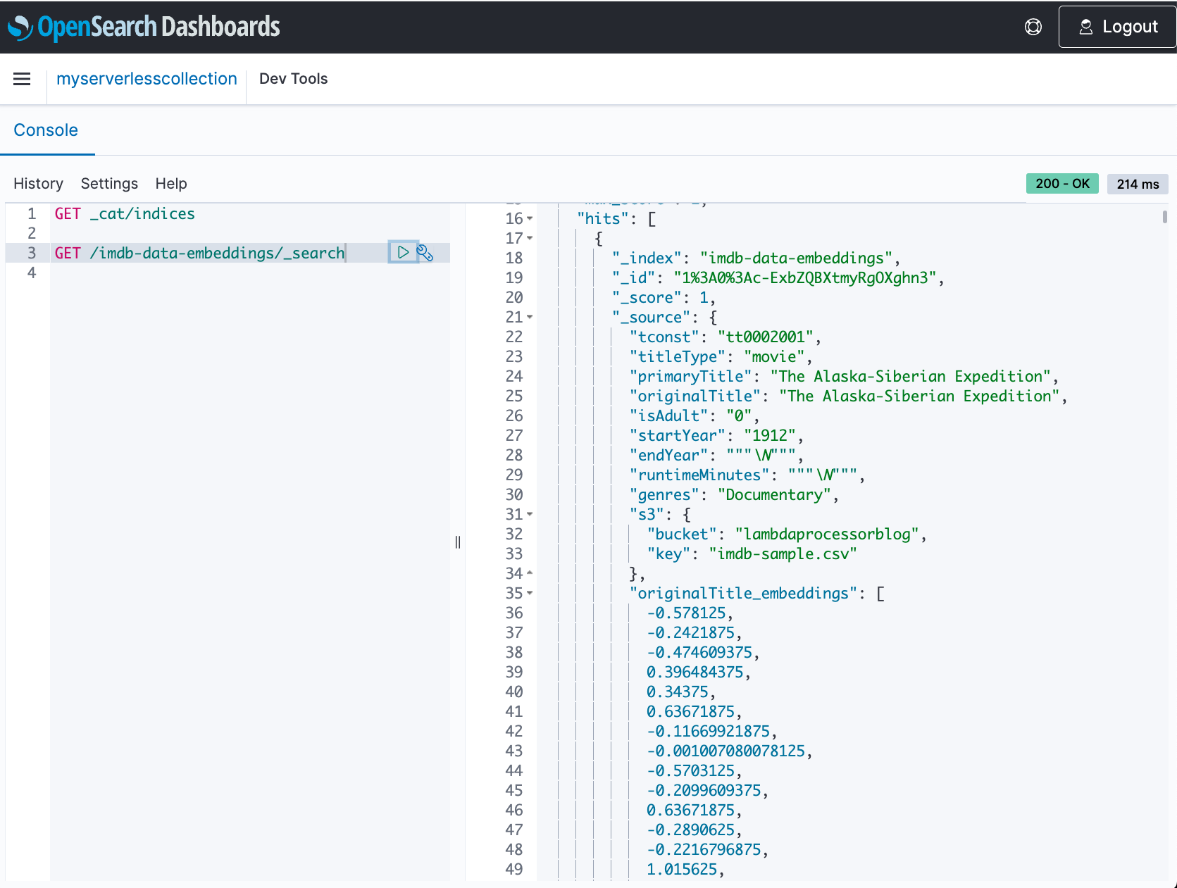
Akash Shankaran is a Software Architect and Tech Lead in the Xeon software team at Intel working on OpenSearch. He works on pathfinding opportunities and enabling optimizations within databases, analytics, and data management domains.

Dylan Tong is a Senior Product Manager at Amazon Web Services. He leads the product initiatives for AI and machine learning (ML) on OpenSearch including OpenSearch’s vector database capabilities. Dylan has decades of experience working directly with customers and creating products and solutions in the database, analytics and AI/ML domain. Dylan holds a BSc and MEng degree in Computer Science from Cornell University.


Notices and disclaimers

Performance varies by use, configuration, and other factors. Learn more on the Performance Index website.
Your costs and results may vary.
Intel technologies may require enabled hardware, software, or service activation.