Tag Archives: Amazon Redshift Spectrum

Accelerate Amazon Redshift Data Lake queries with AWS Glue Data Catalog Column Statistics

2024-10-01 Kalaiselvi Kamaraj

Post Syndicated from Kalaiselvi Kamaraj original https://aws.amazon.com/blogs/big-data/accelerate-amazon-redshift-data-lake-queries-with-column-level-statistics/

Amazon Redshift enables you to efficiently query and retrieve structured and semi-structured data from open format files in Amazon S3 data lake without having to load the data into Amazon Redshift tables. Amazon Redshift extends SQL capabilities to your data lake, enabling you to run analytical queries. Amazon Redshift supports a wide variety of tabular data formats like CSV, JSON, Parquet, ORC and open tabular formats like Apache Hudi, Linux foundation Delta Lake and Apache Iceberg.

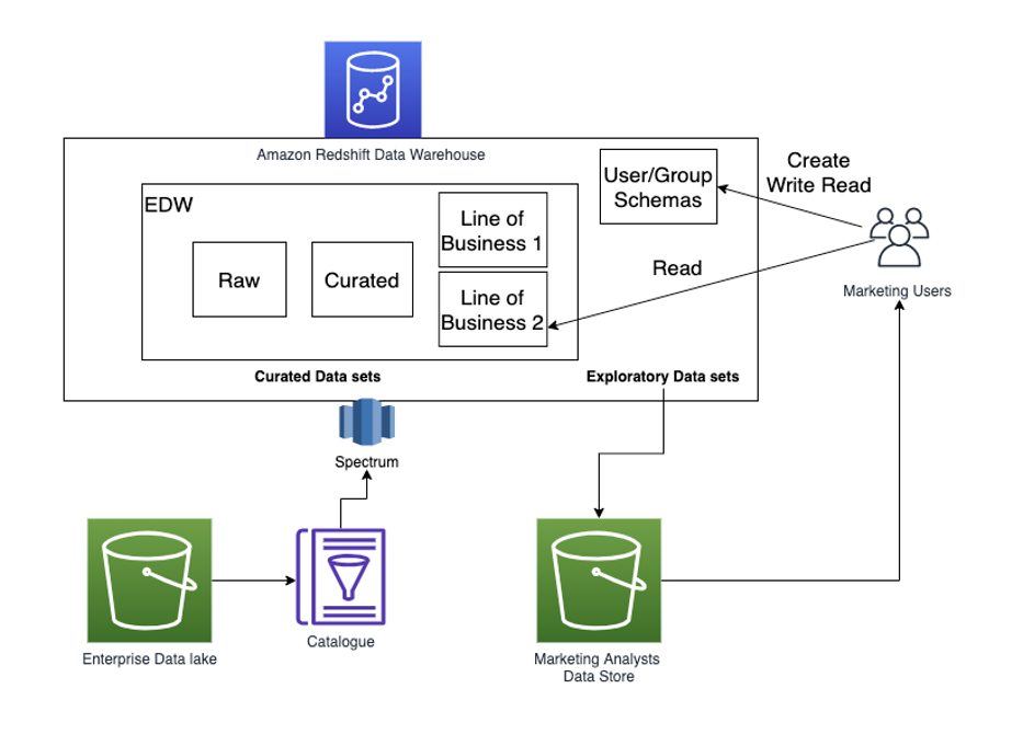
You create Redshift external tables by defining the structure for your files, S3 location of the files and registering them as tables in an external data catalog. The external data catalog can be AWS Glue Data Catalog, the data catalog that comes with Amazon Athena, or your own Apache Hive metastore.

Over the last year, Amazon Redshift added several performance optimizations for data lake queries across multiple areas of query engine such as rewrite, planning, scan execution and consuming AWS Glue Data Catalog column statistics. To get the best performance on data lake queries with Redshift, you can use AWS Glue Data Catalog’s column statistics feature to collect statistics on Data Lake tables. For Amazon Redshift Serverless instances, you will see improved scan performance through increased parallel processing of S3 files and this happens automatically based on RPUs used.

In this post, we highlight the performance improvements we observed using industry standard TPC-DS benchmarks. Overall execution time of TPC-DS 3 TB benchmark improved by 3x. Some of the queries in our benchmark experienced up to 12x speed up.

Performance Improvements

Several performance optimizations were done over the last year to improve performance of data lake queries including the following.

Consume AWS Glue Data Catalog column statistics and tuning of Redshift optimizer to improve quality of query plans
Utilize bloom filters for partition columns
Improved scan efficiency for Amazon Redshift Serverless instances through increased parallel processing of files
Novel query rewrite rules to merge similar scans
Faster retrieval of metadata from AWS Glue Data Catalog

To understand the performance gains, we tested the performance on the industry-standard TPC-DS benchmark using 3 TB data sets and queries which represents different customer use cases. Performance was tested on a Redshift serverless data warehouse with 128 RPU. In our testing, the dataset was stored in Amazon S3 in Parquet format and AWS Glue Data Catalog was used to manage external databases and tables. Fact tables were partitioned on the date column, and each fact table consisted of approximately 2,000 partitions. All of the tables had their row count table property, numRows, set as per the spectrum query performance guidelines.

We did a baseline run on Redshift patch version (patch 172) from last year. Later, we ran all TPC-DS queries on latest patch version (patch 180) that includes all performance optimizations added over last year. Then we used AWS Glue Data Catalog’s column statistics feature to compute statistics for all the tables and measured improvements with the presence of AWS Glue Data Catalog column statistics.

Our analysis revealed that the TPC-DS 3TB Parquet benchmark saw substantial performance gains with these optimizations. Specifically, partitioned Parquet with our latest optimizations achieved 2x faster runtimes compared to the previous implementation. Enabling AWS Glue Data Catalog column statistics further improved performance by 3x versus last year. The following graph illustrates these runtime improvements for the full benchmark (all TPC-DS queries) over the past year, including the additional boost from using AWS Glue Data Catalog column statistics.

Figure 1: Improvement in total runtime of TPC-DS 3T workload

The following graph presents the top queries from the TPC-DS benchmark with the greatest performance improvement over the last year with and without AWS Glue Data Catalog column statistics. You can see that performance improves a lot when statistics exist on AWS Glue Data Catalog (for details on how to get statistics for your Data Lake tables, please refer to optimizing query performance using AWS Glue Data Catalog column statistics). Specifically, multi-join queries will benefit the most from AWS Glue Data Catalog column statistics because the optimizer uses statistics to choose the right join order and distribution strategy.

Figure 2: Speed-up in TPC-DS queries

Let’s discuss some of the optimizations that contributed to improved query performance.

Optimizing with table-level statistics

Amazon Redshift’s design enables it to handle large-scale data challenges with superior speed and cost-efficiency. Its massively parallel processing (MPP) query engine, AI-powered query optimizer, auto-scaling capabilities, and other advanced features allow Redshift to excel at searching, aggregating, and transforming petabytes of data.

However, even the most powerful systems can experience performance degradation if they encounter anti-patterns like grossly inaccurate table statistics, such as the row count metadata.

Without this crucial metadata, Redshift’s query optimizer may be limited in the number of possible optimizations, especially those related to data distribution during query execution. This can have a significant impact on overall query performance.

To illustrate this, consider the following simple query involving an inner join between a large table with billions of rows and a small table with only a few hundred thousand rows.

select small_table.sellerid, sum(large_table.qtysold)
from large_table, small_table
where large_table.salesid = small_table.listid
 and small_table.listtime > '2023-12-01'
 and large_table.saletime > '2023-12-01'
group by 1 order by 1

If executed as-is, with the large table on the right-hand side of the join, the query will lead to sub-optimal performance. This is because the large table will need to be distributed (broadcast) to all Redshift compute nodes to perform the inner join with the small table, as shown in the following diagram.

Inaccurate table statistics lead to limited optimizations and large amounts of data broadcast among compute nodes for a simple inner join

Figure 3: Inaccurate table statistics lead to limited optimizations and large amounts of data broadcast among compute nodes for a simple inner join

Now, consider a scenario where the table statistics, such as the row count, are accurate. This allows the Amazon Redshift query optimizer to make more informed decisions, such as determining the optimal join order. In this case, the optimizer would immediately rewrite the query to have the large table on the left-hand side of the inner join, so that it is the small table that is broadcast across the Redshift compute nodes, as illustrated in the following diagram.

Accurate table statistics lead to high degree of optimizations and very little data broadcast among compute nodes for a simple inner join

Figure 4: Accurate table statistics lead to high degree of optimizations and very little data broadcast among compute nodes for a simple inner join

Fortunately, Amazon Redshift automatically maintains accurate table statistics for local tables by running the ANALYZE command in the background. For external tables (data lake tables), however, AWS Glue Data Catalog column statistics are recommended for use with Amazon Redshift as we will discuss in the next section. For more general information on optimizing queries in Amazon Redshift, please refer to the documentation on factors affecting query performance, data redistribution, and Amazon Redshift best practices for designing queries.

Improvements with AWS Glue Data Catalog column statistics

AWS Glue Data Catalog has a feature to compute column level statistics for Amazon S3 backed external tables. AWS Glue Data Catalog can compute column level statistics such as NDV, Number of Nulls, Min/Max and Avg. column width for the columns without the need for additional data pipelines. Amazon Redshift cost-based optimizer utilizes these statistics to come up with better quality query plans. In addition to consuming statistics, we also made several improvements in cardinality estimations and cost tuning to get high quality query plans thereby improving query performance.

TPC-DS 3TB dataset showed 40% improvement in total query execution time when these AWS Glue Data Catalog column statistics were provided. Individual TPC-DS queries showed up to 5x improvements in query execution time. Some of the queries that had greater impact in execution time are Q85, Q64, Q75, Q78, Q94, Q16, Q04, Q24 and Q11.

We will go through an example where cost-based optimizer generated a better query plan with statistics and how it improved the execution time.

Let’s consider following simpler version of TPC-DS Q64 to showcase the query plan differences with statistics.

select i_product_name product_name
,i_item_sk item_sk
,ad1.ca_street_number b_street_number
,ad1.ca_street_name b_street_name
,ad1.ca_city b_city
,ad1.ca_zip b_zip
,d1.d_year as syear
,count(*) cnt
,sum(ss_wholesale_cost) s1
,sum(ss_list_price) s2
,sum(ss_coupon_amt) s3
FROM   tpcds_3t_alls3_pp_ext.store_sales
,tpcds_3t_alls3_pp_ext.store_returns
,tpcds_3t_alls3_pp_ext.date_dim d1
,tpcds_3t_alls3_pp_ext.customer
,tpcds_3t_alls3_pp_ext.customer_address ad1
,tpcds_3t_alls3_pp_ext.item
WHERE
ss_sold_date_sk = d1.d_date_sk AND
ss_customer_sk = c_customer_sk AND

ss_addr_sk = ad1.ca_address_sk and
ss_item_sk = i_item_sk and
ss_item_sk = sr_item_sk and
ss_ticket_number = sr_ticket_number and
i_color in ('firebrick','papaya','orange','cream','turquoise','deep') and
i_current_price between 42 and 42 + 10 and
i_current_price between 42 + 1 and 42 + 15
group by i_product_name
,i_item_sk
,ad1.ca_street_number
,ad1.ca_street_name
,ad1.ca_city
,ad1.ca_zip
,d1.d_year

Without Statistics

Following figure represents the logical query plan of Q64. You can observe that cardinality estimation of joins is not accurate. With inaccurate cardinalities, optimizer produces a sub-optimal query plan leading to higher execution time.

With Statistics

Following figure represents the logical query plan after consuming AWS Glue Data Catalog column statistics. Based on the highlighted changes, you can observe that the cardinality estimations of JOIN improved by many magnitudes helping the optimizer to choose a better join order and join strategy (broadcast DS_BCAST_INNER vs. distribute DS_DIST_BOTH). Switching the customer_address and customer table from inner to outer table and making join strategies as distribute has major impact because this reduces the data movement between the nodes and avoids spilling from hash table.

Figure 5: Logical query plan of Q64 without statistics

Logical query plan of Q64 after consuming column-level statistics

Figure 6: Logical query plan of Q64 after consuming AWS Glue Data Catalog column statistics

This change in query plan improved the query execution time of Q64 from 383s to 81s.

Given the greater benefits with AWS Glue Data Catalog column statistics for the optimizer, you should consider collecting stats for your data lake using AWS Glue. If your workload is a JOIN heavy workload, then collecting stats will show greater improvement on your workload. Refer to generating AWS Glue Data Catalog column statistics for instructions on how to collect statistics in AWS Glue Data Catalog.

Query rewrite optimization

We introduced a new query rewrite rule which combines scalar aggregates over the same common expression using slightly different predicates. This rewrite resulted in performance improvements on TPC-DS queries Q09, Q28, and Q88. Let’s focus on Q09 as a representative of these queries, given by the following fragment:

SELECT CASE
WHEN (SELECT COUNT(*)
FROM store_sales
WHERE ss_quantity BETWEEN 1 AND 20) > 48409437
THEN (SELECT AVG(ss_ext_discount_amt)
FROM store_sales
WHERE ss_quantity BETWEEN 1 AND 20)
ELSE (SELECT AVG(ss_net_profit)
FROM store_sales
WHERE ss_quantity BETWEEN 1 AND 20) END
AS bucket1,
<<4 more variations of the CASE expression above>>
FROM reason
WHERE r_reason_sk = 1

In total, there are 15 scans of the fact table store_sales, each one returning various aggregates over different subsets of data. The engine first performs subquery removal and transforms the various expressions in the CASE statements into relational subtrees connected via cross products, and then they are fused into one subquery handling all scalar aggregates. The resulting plan for Q09, described below using SQL for clarity, is given by:

SELECT CASE WHEN v1 > 48409437 THEN t1 ELSE e1 END,
<4 more variations>
FROM (SELECT COUNT(CASE WHEN b1 THEN 1 END) AS v1,
AVG(CASE WHEN b1 THEN ss_ext_discount_amt END) AS t1,
AVG(CASE WHEN b1 THEN ss_net_profit END) AS e1,
<4 more variations>
FROM reason,
(SELECT *,
ss_quantity BETWEEN 1 AND 20 AS b1,
<4 more variations>
FROM store_sales
WHERE ss_quantity BETWEEN 1 AND 20 OR
<4 more variations>))
WHERE r_reason_sk = 1)

In general, this rewrite rule results in the largest improvements both in latency (from 3x to 8x improvements) and bytes read from Amazon S3 (from 6x to 8x reduction in scanned bytes and, consequently, cost).

Bloom filter for partition columns

Amazon Redshift already uses Bloom filters on data columns of external tables in Amazon S3 to enable early and effective data filtering. Last year, we extended this support for partition columns as well. A Bloom filter is a probabilistic, memory-efficient data structure that accelerates join queries at scale by filtering rows that do not match the join relation, significantly reducing the amount of data transferred over the network. Amazon Redshift automatically determines what queries are suitable for leveraging Bloom filters at query runtime.

This optimization resulted in performance improvements on TPC-DS queries Q05, Q17 and Q54. This optimization resulted in large improvements in both latency (from 2x to 3x improvement) and bytes read from S3 (from 9x to 15x reduction in scanned bytes and, consequently cost).

Following is the subquery of Q05 which showcased improvements with runtime filter.

select s_store_id,
sum(sales_price) as sales,
sum(profit) as profit,
sum(return_amt) as returns,
sum(net_loss) as profit_loss
from
( select  ss_store_sk as store_sk,
ss_sold_date_sk  as date_sk,
ss_ext_sales_price as sales_price,
ss_net_profit as profit,
cast(0 as decimal(7,2)) as return_amt,
cast(0 as decimal(7,2)) as net_loss
from tpcds_3t_alls3_pp_ext.store_sales
union all
select sr_store_sk as store_sk,
sr_returned_date_sk as date_sk,
cast(0 as decimal(7,2)) as sales_price,
cast(0 as decimal(7,2)) as profit,
sr_return_amt as return_amt,
sr_net_loss as net_loss
from tpcds_3t_alls3_pp_ext.store_returns
) salesreturnss,
tpcds_3t_alls3_pp_ext.date_dim,
tpcds_3t_alls3_pp_ext.store
where date_sk = d_date_sk
and d_date between cast('1998-08-13' as date)
and (cast('1998-08-13' as date) +  14)
and store_sk = s_store_sk
group by s_store_id

Without bloom filter support on partition columns

Following figure is the logical query plan for sub-query of Q05. This appends two large fact tables store_sales (8B rows) and store_returns (863M rows) and then joins with very selective dimension tables date_dim and then with dimension table store. You can observe that join with date_dim table reduces the number of rows from 9B to 93M rows.

With bloom filter support on partition columns

With support of bloom filter on partition columns, we now create bloom filter for d_date_sk column of date_dim table and push down the bloom filters to store_sales and store_returns table. These bloom filters help to filter out the partitions in both store_sales and store_returns table because join happens on partition column (number of partitions processed reduces by 10x).

Figure 7: Logical query plan for sub-query of Q05 without bloom filter support on partition columns

Figure 8: Logical query plan for sub-query of Q05 with bloom filter support on partition columns

Overall, bloom filter on partition column will reduce the number of partitions processed resulting in reduced S3 listing calls and lesser number of data files to be read (reduction in scanned bytes). You can see that we only scan 89M rows from store_sales and 4M rows from store_returns because of the bloom filter. This reduced number of rows to process at JOIN level and helped in improving the overall query performance by 2x and scanned bytes by 9x.

Conclusion

In this post, we covered new performance optimizations in Amazon Redshift data lake query processing and how AWS Glue Data Catalog statistics helps to enhance quality of query plans for data lake queries in Amazon Redshift. These optimizations together improved TPC-DS 3 TB benchmark by 3x. Some of the queries in our benchmark benefited up to 12x speed up.

In summary, Amazon Redshift now offers enhanced query performance with optimizations such as AWS Glue Data Catalog column statistics, bloom filters on partition columns, new query rewrite rules and faster retrieval of metadata. These optimizations are enabled by default and Amazon Redshift users will benefit with better query response times for their workloads. For more information, please reach out to your AWS technical account manager or AWS account solutions architect. They will be happy to provide additional guidance and support.

About the authors

Kalaiselvi Kamaraj is a Sr. Software Development Engineer with Amazon. She has worked on several projects within Redshift Query processing team and currently focusing on performance related projects for Redshift Data Lake.

Mark Lyons is a Principal Product Manager on the Amazon Redshift team. He works on the intersection of data lakes and data warehouses. Prior to joining AWS, Mark held product leadership roles with Dremio and Vertica. He is passionate about data analytics and empowering customers to change the world with their data.

Asser Moustafa is a Principal Worldwide Specialist Solutions Architect at AWS, based in Dallas, Texas, USA. He partners with customers worldwide, advising them on all aspects of their data architectures, migrations, and strategic data visions to help organizations adopt cloud-based solutions, maximize the value of their data assets, modernize legacy infrastructures, and implement cutting-edge capabilities like machine learning and advanced analytics. Prior to joining AWS, Asser held various data and analytics leadership roles, completing an MBA from New York University and an MS in Computer Science from Columbia University in New York. He is passionate about empowering organizations to become truly data-driven and unlock the transformative potential of their data.

Seamless integration of data lake and data warehouse using Amazon Redshift Spectrum and Amazon DataZone

2024-08-15 Lakshmi Nair

Post Syndicated from Lakshmi Nair original https://aws.amazon.com/blogs/big-data/seamless-integration-of-data-lake-and-data-warehouse-using-amazon-redshift-spectrum-and-amazon-datazone/

Unlocking the true value of data often gets impeded by siloed information. Traditional data management—wherein each business unit ingests raw data in separate data lakes or warehouses—hinders visibility and cross-functional analysis. A data mesh framework empowers business units with data ownership and facilitates seamless sharing.

However, integrating datasets from different business units can present several challenges. Each business unit exposes data assets with varying formats and granularity levels, and applies different data validation checks. Unifying these necessitates additional data processing, requiring each business unit to provision and maintain a separate data warehouse. This burdens business units focused solely on consuming the curated data for analysis and not concerned with data management tasks, cleansing, or comprehensive data processing.

In this post, we explore a robust architecture pattern of a data sharing mechanism by bridging the gap between data lake and data warehouse using Amazon DataZone and Amazon Redshift.

Solution overview

Amazon DataZone is a data management service that makes it straightforward for business units to catalog, discover, share, and govern their data assets. Business units can curate and expose their readily available domain-specific data products through Amazon DataZone, providing discoverability and controlled access.

Amazon Redshift is a fast, scalable, and fully managed cloud data warehouse that allows you to process and run your complex SQL analytics workloads on structured and semi-structured data. Thousands of customers use Amazon Redshift data sharing to enable instant, granular, and fast data access across Amazon Redshift provisioned clusters and serverless workgroups. This allows you to scale your read and write workloads to thousands of concurrent users without having to move or copy the data. Amazon DataZone natively supports data sharing for Amazon Redshift data assets. With Amazon Redshift Spectrum, you can query the data in your Amazon Simple Storage Service (Amazon S3) data lake using a central AWS Glue metastore from your Redshift data warehouse. This capability extends your petabyte-scale Redshift data warehouse to unbounded data storage limits, which allows you to scale to exabytes of data cost-effectively.

The following figure shows a typical distributed and collaborative architectural pattern implemented using Amazon DataZone. Business units can simply share data and collaborate by publishing and subscribing to the data assets.

hubandspoke

The Central IT team (Spoke N) subscribes the data from individual business units and consumes this data using Redshift Spectrum. The Central IT team applies standardization and performs the tasks on the subscribed data such as schema alignment, data validation checks, collating the data, and enrichment by adding additional context or derived attributes to the final data asset. This processed unified data can then persist as a new data asset in Amazon Redshift managed storage to meet the SLA requirements of the business units. The new processed data asset produced by the Central IT team is then published back to Amazon DataZone. With Amazon DataZone, individual business units can discover and directly consume these new data assets, gaining insights to a holistic view of the data (360-degree insights) across the organization.

The Central IT team manages a unified Redshift data warehouse, handling all data integration, processing, and maintenance. Business units access clean, standardized data. To consume the data, they can choose between a provisioned Redshift cluster for consistent high-volume needs or Amazon Redshift Serverless for variable, on-demand analysis. This model enables the units to focus on insights, with costs aligned to actual consumption. This allows the business units to derive value from data without the burden of data management tasks.

This streamlined architecture approach offers several advantages:

Single source of truth – The Central IT team acts as the custodian of the combined and curated data from all business units, thereby providing a unified and consistent dataset. The Central IT team implements data governance practices, providing data quality, security, and compliance with established policies. A centralized data warehouse for processing is often more cost-efficient, and its scalability allows organizations to dynamically adjust their storage needs. Similarly, individual business units produce their own domain-specific data. There are no duplicate data products created by business units or the Central IT team.
Eliminating dependency on business units – Redshift Spectrum uses a metadata layer to directly query the data residing in S3 data lakes, eliminating the need for data copying or relying on individual business units to initiate the copy jobs. This significantly reduces the risk of errors associated with data transfer or movement and data copies.
Eliminating stale data – Avoiding duplication of data also eliminates the risk of stale data existing in multiple locations.
Incremental loading – Because the Central IT team can directly query the data on the data lakes using Redshift Spectrum, they have the flexibility to query only the relevant columns needed for the unified analysis and aggregations. This can be done using mechanisms to detect the incremental data from the data lakes and process only the new or updated data, further optimizing resource utilization.
Federated governance – Amazon DataZone facilitates centralized governance policies, providing consistent data access and security across all business units. Sharing and access controls remain confined within Amazon DataZone.
Enhanced cost appropriation and efficiency – This method confines the cost overhead of processing and integrating the data with the Central IT team. Individual business units can provision the Redshift Serverless data warehouse to solely consume the data. This way, each unit can clearly demarcate the consumption costs and impose limits. Additionally, the Central IT team can choose to apply chargeback mechanisms to each of these units.

In this post, we use a simplified use case, as shown in the following figure, to bridge the gap between data lakes and data warehouses using Redshift Spectrum and Amazon DataZone.

custom blueprints and spectrum

The underwriting business unit curates the data asset using AWS Glue and publishes the data asset Policies in Amazon DataZone. The Central IT team subscribes to the data asset from the underwriting business unit.

We focus on how the Central IT team consumes the subscribed data lake asset from business units using Redshift Spectrum and creates a new unified data asset.

Prerequisites

The following prerequisites must be in place:

AWS accounts – You should have active AWS accounts before you proceed. If you don’t have one, refer to How do I create and activate a new AWS account? In this post, we use three AWS accounts. If you’re new to Amazon DataZone, refer to Getting started.
A Redshift data warehouse – You can create a provisioned cluster following the instructions in Create a sample Amazon Redshift cluster, or provision a serverless workgroup following the instructions in Get started with Amazon Redshift Serverless data warehouses.
Amazon Data Zone resources – You need a domain for Amazon DataZone, an Amazon DataZone project, and a new Amazon DataZone environment (with a custom AWS service blueprint).
Data lake asset – The data lake asset Policies from the business units was already onboarded to Amazon DataZone and subscribed by the Central IT team. To understand how to associate multiple accounts and consume the subscribed assets using Amazon Athena, refer to Working with associated accounts to publish and consume data.
Central IT environment – The Central IT team has created an environment called env_central_team and uses an existing AWS Identity and Access Management (IAM) role called custom_role, which grants Amazon DataZone access to AWS services and resources, such as Athena, AWS Glue, and Amazon Redshift, in this environment. To add all the subscribed data assets to a common AWS Glue database, the Central IT team configures a subscription target and uses central_db as the AWS Glue database.
IAM role – Make sure that the IAM role that you want to enable in the Amazon DataZone environment has necessary permissions to your AWS services and resources. The following example policy provides sufficient AWS Lake Formation and AWS Glue permissions to access Redshift Spectrum:

{
	"Version": "2012-10-17",
	"Statement": [{
		"Effect": "Allow",
		"Action": [
			"lakeformation:GetDataAccess",
			"glue:GetTable",
			"glue:GetTables",
			"glue:SearchTables",
			"glue:GetDatabase",
			"glue:GetDatabases",
			"glue:GetPartition",
			"glue:GetPartitions"
		],
		"Resource": "*"
	}]
}

As shown in the following screenshot, the Central IT team has subscribed to the data Policies. The data asset is added to the env_central_team environment. Amazon DataZone will assume the custom_role to help federate the environment user (central_user) to the action link in Athena. The subscribed asset Policies is added to the central_db database. This asset is then queried and consumed using Athena.

The goal of the Central IT team is to consume the subscribed data lake asset Policies with Redshift Spectrum. This data is further processed and curated into the central data warehouse using the Amazon Redshift Query Editor v2 and stored as a single source of truth in Amazon Redshift managed storage. In the following sections, we illustrate how to consume the subscribed data lake asset Policies from Redshift Spectrum without copying the data.

Automatically mount access grants to the Amazon DataZone environment role

Amazon Redshift automatically mounts the AWS Glue Data Catalog in the Central IT Team account as a database and allows it to query the data lake tables with three-part notation. This is available by default with the Admin role.

To grant the required access to the mounted Data Catalog tables for the environment role (custom_role), complete the following steps:

Log in to the Amazon Redshift Query Editor v2 using the Amazon DataZone deep link.
In the Query Editor v2, choose your Redshift Serverless endpoint and choose Edit Connection.
For Authentication, select Federated user.
For Database, enter the database you want to connect to.
Get the current user IAM role as illustrated in the following screenshot.

getcurrentUser from Redshift QEv2

Connect to Redshift Query Editor v2 using the database user name and password authentication method. For example, connect to dev database using the admin user name and password. Grant usage on the awsdatacatalog database to the environment user role custom_role (replace the value of current_user with the value you copied):

GRANT USAGE ON DATABASE awsdatacatalog to "IAMR:current_user"

Query using Redshift Spectrum

Using the federated user authentication method, log in to Amazon Redshift. The Central IT team will be able to query the subscribed data asset Policies (table: policy) that was automatically mounted under awsdatacatalog.

query with spectrum

Aggregate tables and unify products

The Central IT team applies the necessary checks and standardization to aggregate and unify the data assets from all business units, bringing them at the same granularity. As shown in the following screenshot, both the Policies and Claims data assets are combined to form a unified aggregate data asset called agg_fraudulent_claims.

creatingunified product

These unified data assets are then published back to the Amazon DataZone central hub for business units to consume them.

unified asset published

The Central IT team also unloads the data assets to Amazon S3 so that each business unit has the flexibility to use either a Redshift Serverless data warehouse or Athena to consume the data. Each business unit can now isolate and put limits to the consumption costs on their individual data warehouses.

Because the intention of the Central IT team was to consume data lake assets within a data warehouse, the recommended solution would be to use custom AWS service blueprints and deploy them as part of one environment. In this case, we created one environment (env_central_team) to consume the asset using Athena or Amazon Redshift. This accelerates the development of the data sharing process because the same environment role is used to manage the permissions across multiple analytical engines.

Clean up

To clean up your resources, complete the following steps:

Delete any S3 buckets you created.
On the Amazon DataZone console, delete the projects used in this post. This will delete most project-related objects like data assets and environments.
Delete the Amazon DataZone domain.
On the Lake Formation console, delete the Lake Formation admins registered by Amazon DataZone along with the tables and databases created by Amazon DataZone.
If you used a provisioned Redshift cluster, delete the cluster. If you used Redshift Serverless, delete any tables created as part of this post.

Conclusion

In this post, we explored a pattern of seamless data sharing with data lakes and data warehouses with Amazon DataZone and Redshift Spectrum. We discussed the challenges associated with traditional data management approaches, data silos, and the burden of maintaining individual data warehouses for business units.

In order to curb operating and maintenance costs, we proposed a solution that uses Amazon DataZone as a central hub for data discovery and access control, where business units can readily share their domain-specific data. To consolidate and unify the data from these business units and provide a 360-degree insight, the Central IT team uses Redshift Spectrum to directly query and analyze the data residing in their respective data lakes. This eliminates the need for creating separate data copy jobs and duplication of data residing in multiple places.

The team also takes on the responsibility of bringing all the data assets to the same granularity and process a unified data asset. These combined data products can then be shared through Amazon DataZone to these business units. Business units can only focus on consuming the unified data assets that aren’t specific to their domain. This way, the processing costs can be controlled and tightly monitored across all business units. The Central IT team can also implement chargeback mechanisms based on the consumption of the unified products for each business unit.

To learn more about Amazon DataZone and how to get started, refer to Getting started. Check out the YouTube playlist for some of the latest demos of Amazon DataZone and more information about the capabilities available.

About the Authors

Lakshmi Nair is a Senior Analytics Specialist Solutions Architect at AWS. She specializes in designing advanced analytics systems across industries. She focuses on crafting cloud-based data platforms, enabling real-time streaming, big data processing, and robust data governance.

Srividya Parthasarathy is a Senior Big Data Architect on the AWS Lake Formation team. She enjoys building analytics and data mesh solutions on AWS and sharing them with the community.

Create, train, and deploy Amazon Redshift ML model integrating features from Amazon SageMaker Feature Store

2023-10-26 Anirban Sinha

Post Syndicated from Anirban Sinha original https://aws.amazon.com/blogs/big-data/create-train-and-deploy-amazon-redshift-ml-model-integrating-features-from-amazon-sagemaker-feature-store/

Amazon Redshift is a fast, petabyte-scale, cloud data warehouse that tens of thousands of customers rely on to power their analytics workloads. Data analysts and database developers want to use this data to train machine learning (ML) models, which can then be used to generate insights on new data for use cases such as forecasting revenue, predicting customer churn, and detecting anomalies. Amazon Redshift ML makes it easy for SQL users to create, train, and deploy ML models using SQL commands familiar to many roles such as executives, business analysts, and data analysts. We covered in a previous post how you can use data in Amazon Redshift to train models in Amazon SageMaker, a fully managed ML service, and then make predictions within your Redshift data warehouse.

Redshift ML currently supports ML algorithms such as XGBoost, multilayer perceptron (MLP), KMEANS, and Linear Learner. Additionally, you can import existing SageMaker models into Amazon Redshift for in-database inference or remotely invoke a SageMaker endpoint.

Amazon SageMaker Feature Store is a fully managed, purpose-built repository to store, share, and manage features for ML models. However, one challenge in training a production-ready ML model using SageMaker Feature Store is access to a diverse set of features that aren’t always owned and maintained by the team that is building the model. For example, an ML model to identify fraudulent financial transactions needs access to both identifying (device type, browser) and transaction (amount, credit or debit, and so on) related features. As a data scientist building an ML model, you may have access to the identifying information but not the transaction information, and having access to a feature store solves this.

In this post, we discuss the combined feature store pattern, which allows teams to maintain their own local feature stores using a local Redshift table while still being able to access shared features from the centralized feature store. In a local feature store, you can store sensitive data that can’t be shared across the organization for regulatory and compliance reasons.

We also show you how to use familiar SQL statements to create and train ML models by combining shared features from the centralized store with local features and use these models to make in-database predictions on new data for use cases such as fraud risk scoring.

Overview of solution

For this post, we create an ML model to predict if a transaction is fraudulent or not, given the transaction record. To build this, we need to engineer features that describe an individual credit card’s spending pattern, such as the number of transactions or the average transaction amount, and also information about the merchant, the cardholder, the device used to make the payment, and any other data that may be relevant to detecting fraud.

To get started, we need an Amazon Redshift Serverless data warehouse with the Redshift ML feature enabled and an Amazon SageMaker Studio environment with access to SageMaker Feature Store. For an introduction to Redshift ML and instructions on setting it up, see Create, train, and deploy machine learning models in Amazon Redshift using SQL with Amazon Redshift ML.

We also need an offline feature store to store features in feature groups. The offline store uses an Amazon Simple Storage Service (Amazon S3) bucket for storage and can also fetch data using Amazon Athena queries. For an introduction to SageMaker Feature Store and instructions on setting it up, see Getting started with Amazon SageMaker Feature Store.

The following diagram illustrates solution architecture.

The workflow contains the following steps:

Create the offline feature group in SageMaker Feature Store and ingest data into the feature group.
Create a Redshift table and load local feature data into the table.
Create an external schema for Amazon Redshift Spectrum to access the offline store data stored in Amazon S3 using the AWS Glue Data Catalog.
Train and validate a fraud risk scoring ML model using local feature data and external offline feature store data.
Use the offline feature store and local store for inference.

Dataset

To demonstrate this use case, we use a synthetic dataset with two tables: identity and transactions. They can both be joined by the TransactionID column. The transaction table contains information about a particular transaction, such as amount, credit or debit card, and so on, and the identity table contains information about the user, such as device type and browser. The transaction must exist in the transaction table, but might not always be available in the identity table.

The following is an example of the transactions dataset.

The following is an example of the identity dataset.

Let’s assume that across the organization, data science teams centrally manage the identity data and process it to extract features in a centralized offline feature store. The data warehouse team ingests and analyzes transaction data in a Redshift table, owned by them.

We work through this use case to understand how the data warehouse team can securely retrieve the latest features from the identity feature group and join it with transaction data in Amazon Redshift to create a feature set for training and inferencing a fraud detection model.

Create the offline feature group and ingest data

To start, we set up SageMaker Feature Store, create a feature group for the identity dataset, inspect and process the dataset, and ingest some sample data. We then prepare the transaction features from the transaction data and store it in Amazon S3 for further loading into the Redshift table.

Alternatively, you can author features using Amazon SageMaker Data Wrangler, create feature groups in SageMaker Feature Store, and ingest features in batches using an Amazon SageMaker Processing job with a notebook exported from SageMaker Data Wrangler. This mode allows for batch ingestion into the offline store.

Let’s explore some of the key steps in this section.

Download the sample notebook.
On the SageMaker console, under Notebook in the navigation pane, choose Notebook instances.
Locate your notebook instance and choose Open Jupyter.
Choose Upload and upload the notebook you just downloaded.
Open the notebook sagemaker_featurestore_fraud_redshiftml_python_sdk.ipynb.
Follow the instructions and run all the cells up to the Cleanup Resources section.

The following are key steps from the notebook:

We create a Pandas DataFrame with the initial CSV data. We apply feature transformations for this dataset.

identity_data = pd.read_csv(io.BytesIO(identity_data_object["Body"].read()))
transaction_data = pd.read_csv(io.BytesIO(transaction_data_object["Body"].read()))

identity_data = identity_data.round(5)
transaction_data = transaction_data.round(5)

identity_data = identity_data.fillna(0)
transaction_data = transaction_data.fillna(0)

# Feature transformations for this dataset are applied 
# One hot encode card4, card6
encoded_card_bank = pd.get_dummies(transaction_data["card4"], prefix="card_bank")
encoded_card_type = pd.get_dummies(transaction_data["card6"], prefix="card_type")

transformed_transaction_data = pd.concat(
    [transaction_data, encoded_card_type, encoded_card_bank], axis=1
)

We store the processed and transformed transaction dataset in an S3 bucket. This transaction data will be loaded later in the Redshift table for building the local feature store.

transformed_transaction_data.to_csv("transformed_transaction_data.csv", header=False, index=False)
s3_client.upload_file("transformed_transaction_data.csv", default_s3_bucket_name, prefix + "/training_input/transformed_transaction_data.csv")

Next, we need a record identifier name and an event time feature name. In our fraud detection example, the column of interest is TransactionID.EventTime can be appended to your data when no timestamp is available. In the following code, you can see how these variables are set, and then EventTime is appended to both features’ data.
```
# record identifier and event time feature names
record_identifier_feature_name = "TransactionID"
event_time_feature_name = "EventTime"

# append EventTime feature
identity_data[event_time_feature_name] = pd.Series(
    [current_time_sec] * len(identity_data), dtype="float64"
)
```

We then create and ingest the data into the feature group using the SageMaker SDK FeatureGroup.ingest API. This is a small dataset and therefore can be loaded into a Pandas DataFrame. When we work with large amounts of data and millions of rows, there are other scalable mechanisms to ingest data into SageMaker Feature Store, such as batch ingestion with Apache Spark.

identity_feature_group.create(
    s3_uri=<S3_Path_Feature_Store>,
    record_identifier_name=record_identifier_feature_name,
    event_time_feature_name=event_time_feature_name,
    role_arn=<role_arn>,
    enable_online_store=False,
)

identity_feature_group_name = "identity-feature-group"

# load feature definitions to the feature group. SageMaker FeatureStore Python SDK will auto-detect the data schema based on input data.
identity_feature_group.load_feature_definitions(data_frame=identity_data)
identity_feature_group.ingest(data_frame=identity_data, max_workers=3, wait=True)

We can verify that data has been ingested into the feature group by running Athena queries in the notebook or running queries on the Athena console.

At this point, the identity feature group is created in an offline feature store with historical data persisted in Amazon S3. SageMaker Feature Store automatically creates an AWS Glue Data Catalog for the offline store, which enables us to run SQL queries against the offline data using Athena or Redshift Spectrum.

Create a Redshift table and load local feature data

To build a Redshift ML model, we build a training dataset joining the identity data and transaction data using SQL queries. The identity data is in a centralized feature store where the historical set of records are persisted in Amazon S3. The transaction data is a local feature for training data that needs to made available in the Redshift table.

Let’s explore how to create the schema and load the processed transaction data from Amazon S3 into a Redshift table.

Create the customer_transaction table and load daily transaction data into the table, which you’ll use to train the ML model:

DROP TABLE customer_transaction;
CREATE TABLE customer_transaction (
  TransactionID INT,    
  isFraud INT,  
  TransactionDT INT,    
  TransactionAmt decimal(10,2), 
  card1 INT,    
  card2 decimal(10,2),card3 decimal(10,2),  
  card4 VARCHAR(20),card5 decimal(10,2),    
  card6 VARCHAR(20),    
  B1 INT,B2 INT,B3 INT,B4 INT,B5 INT,B6 INT,
  B7 INT,B8 INT,B9 INT,B10 INT,B11 INT,B12 INT,
  F1 INT,F2 INT,F3 INT,F4 INT,F5 INT,F6 INT,
  F7 INT,F8 INT,F9 INT,F10 INT,F11 INT,F12 INT,
  F13 INT,F14 INT,F15 INT,F16 INT,F17 INT,  
  N1 VARCHAR(20),N2 VARCHAR(20),N3 VARCHAR(20), 
  N4 VARCHAR(20),N5 VARCHAR(20),N6 VARCHAR(20), 
  N7 VARCHAR(20),N8 VARCHAR(20),N9 VARCHAR(20), 
  card_type_0  boolean,
  card_type_credit boolean,
  card_type_debit  boolean,
  card_bank_0  boolean,
  card_bank_american_express boolean,
  card_bank_discover  boolean,
  card_bank_mastercard  boolean,
  card_bank_visa boolean  
);

Load the sample data by using the following command. Replace your Region and S3 path as appropriate. You will find the S3 path in the S3 Bucket Setup For The OfflineStore section in the notebook or by checking the dataset_uri_prefix in the notebook.
```
COPY customer_transaction
FROM '<s3path>/transformed_transaction_data.csv' 
IAM_ROLE default delimiter ',' 
region 'your-region';
```

Now that we have created a local feature store for the transaction data, we focus on integrating a centralized feature store with Amazon Redshift to access the identity data.

Create an external schema for Redshift Spectrum to access the offline store data

We have created a centralized feature store for identity features, and we can access this offline feature store using services such as Redshift Spectrum. When the identity data is available through the Redshift Spectrum table, we can create a training dataset with feature values from the identity feature group and customer_transaction, joining on the TransactionId column.

This section provides an overview of how to enable Redshift Spectrum to query data directly from files on Amazon S3 through an external database in an AWS Glue Data Catalog.

First, check that the identity-feature-group table is present in the Data Catalog under the sagemamker_featurestore database.

Using Redshift Query Editor V2, create an external schema using the following command:

CREATE EXTERNAL SCHEMA sagemaker_featurestore
FROM DATA CATALOG
DATABASE 'sagemaker_featurestore'
IAM_ROLE default
create external database if not exists;

All the tables, including identity-feature-group external tables, are visible under the sagemaker_featurestore external schema. In Redshift Query Editor v2, you can check the contents of the external schema.

Run the following query to sample a few records—note that your table name may be different:
```
Select * from sagemaker_featurestore.identity_feature_group_1680208535 limit 10;
```

Create a view to join the latest data from identity-feature-group and customer_transaction on the TransactionId column. Be sure to change the external table name to match your external table name:

create or replace view public.credit_fraud_detection_v
AS select  "isfraud",
        "transactiondt",
        "transactionamt",
        "card1","card2","card3","card5",
         case when "card_type_credit" = 'False' then 0 else 1 end as card_type_credit,
         case when "card_type_debit" = 'False' then 0 else 1 end as card_type_debit,
         case when "card_bank_american_express" = 'False' then 0 else 1 end as card_bank_american_express,
         case when "card_bank_discover" = 'False' then 0 else 1 end as card_bank_discover,
         case when "card_bank_mastercard" = 'False' then 0 else 1 end as card_bank_mastercard,
         case when "card_bank_visa" = 'False' then 0 else 1 end as card_bank_visa,
        "id_01","id_02","id_03","id_04","id_05"
from public.customer_transaction ct left join sagemaker_featurestore.identity_feature_group_1680208535 id
on id.transactionid = ct.transactionid with no schema binding;

Train and validate the fraud risk scoring ML model

Redshift ML gives you the flexibility to specify your own algorithms and model types and also to provide your own advanced parameters, which can include preprocessors, problem type, and hyperparameters. In this post, we create a customer model by specifying AUTO OFF and the model type of XGBOOST. By turning AUTO OFF and using XGBoost, we are providing the necessary inputs for SageMaker to train the model. A benefit of this can be faster training times. XGBoost is as open-source version of the gradient boosted trees algorithm. For more details on XGBoost, refer to Build XGBoost models with Amazon Redshift ML.

We train the model using 80% of the dataset by filtering on transactiondt < 12517618. The other 20% will be used for inference. A centralized feature store is useful in providing the latest supplementing data for training requests. Note that you will need to provide an S3 bucket name in the create model statement. It will take approximately 10 minutes to create the model.

CREATE MODEL frauddetection_xgboost
FROM (select  "isfraud",
        "transactiondt",
        "transactionamt",
        "card1","card2","card3","card5",
        "card_type_credit",
        "card_type_debit",
        "card_bank_american_express",
        "card_bank_discover",
        "card_bank_mastercard",
        "card_bank_visa",
        "id_01","id_02","id_03","id_04","id_05"
from credit_fraud_detection_v where transactiondt < 12517618
)
TARGET isfraud
FUNCTION ml_fn_frauddetection_xgboost
IAM_ROLE default
AUTO OFF
MODEL_TYPE XGBOOST
OBJECTIVE 'binary:logistic'
PREPROCESSORS 'none'
HYPERPARAMETERS DEFAULT EXCEPT(NUM_ROUND '100')
SETTINGS (S3_BUCKET <s3_bucket>);

When you run the create model command, it will complete quickly in Amazon Redshift while the model training is happening in the background using SageMaker. You can check the status of the model by running a show model command:

show model frauddetection_xgboost;

The output of the show model command shows that the model state is TRAINING. It also shows other information such as the model type and the training job name that SageMaker assigned.
After a few minutes, we run the show model command again:

show model frauddetection_xgboost;

Now the output shows the model state is READY. We can also see the train:error score here, which at 0 tells us we have a good model. Now that the model is trained, we can use it for running inference queries.

Use the offline feature store and local store for inference

We can use the SQL function to apply the ML model to data in queries, reports, and dashboards. Let’s use the function ml_fn_frauddetection_xgboost created by our model against our test dataset by filtering where transactiondt >=12517618, to predict whether a transaction is fraudulent or not. SageMaker Feature Store can be useful in supplementing data for inference requests.

Run the following query to predict whether transactions are fraudulent or not:

select  "isfraud" as "Actual",
        ml_fn_frauddetection_xgboost(
        "transactiondt",
        "transactionamt",
        "card1","card2","card3","card5",
        "card_type_credit",
        "card_type_debit",
        "card_bank_american_express",
        "card_bank_discover",
        "card_bank_mastercard",
        "card_bank_visa",
        "id_01","id_02","id_03","id_04","id_05") as "Predicted"
from credit_fraud_detection_v where transactiondt >= 12517618;

For binary and multi-class classification problems, we compute the accuracy as the model metric. Accuracy can be calculated based on the following:

accuracy = (sum (actual == predicted)/total) *100

Let’s apply the preceding code to our use case to find the accuracy of the model. We use the test data (transactiondt >= 12517618) to test the accuracy, and use the newly created function ml_fn_frauddetection_xgboost to predict and take the columns other than the target and label as the input:

-- check accuracy 
WITH infer_data AS (
SELECT "isfraud" AS label,
ml_fn_frauddetection_xgboost(
        "transactiondt",
        "transactionamt",
        "card1","card2","card3","card5",
        "card_type_credit",
        "card_type_debit",
        "card_bank_american_express",
        "card_bank_discover",
        "card_bank_mastercard",
        "card_bank_visa",
        "id_01","id_02","id_03","id_04","id_05") AS predicted,
CASE 
   WHEN label IS NULL
       THEN 0
   ELSE label
   END AS actual,
CASE 
   WHEN actual = predicted
       THEN 1::INT
   ELSE 0::INT
   END AS correct
FROM credit_fraud_detection_v where transactiondt >= 12517618),
aggr_data AS (
SELECT SUM(correct) AS num_correct,
COUNT(*) AS total
FROM infer_data) 

SELECT (num_correct::FLOAT / total::FLOAT) AS accuracy FROM aggr_data;

Clean up

As a final step, clean up the resources:

Delete the Redshift cluster.
Run the Cleanup Resources section of your notebook.

Conclusion

Redshift ML enables you to bring machine learning to your data, powering fast and informed decision-making. SageMaker Feature Store provides a purpose-built feature management solution to help organizations scale ML development across business units and data science teams.

In this post, we showed how you can train an XGBoost model using Redshift ML with data spread across SageMaker Feature Store and a Redshift table. Additionally, we showed how you can make inferences on a trained model to detect fraud using Amazon Redshift SQL commands.

About the authors

Anirban Sinha is a Senior Technical Account Manager at AWS. He is passionate about building scalable data warehouses and big data solutions working closely with customers. He works with large ISVs customers, in helping them build and operate secure, resilient, scalable, and high-performance SaaS applications in the cloud.

Phil Bates is a Senior Analytics Specialist Solutions Architect at AWS. He has more than 25 years of experience implementing large-scale data warehouse solutions. He is passionate about helping customers through their cloud journey and using the power of ML within their data warehouse.

Gaurav Singh is a Senior Solutions Architect at AWS, specializing in AI/ML and Generative AI. Based in Pune, India, he focuses on helping customers build, deploy, and migrate ML production workloads to SageMaker at scale. In his spare time, Gaurav loves to explore nature, read, and run.

Automate data archival for Amazon Redshift time series tables

2022-10-04 Nita Shah

Post Syndicated from Nita Shah original https://aws.amazon.com/blogs/big-data/automate-data-archival-for-amazon-redshift-time-series-tables/

Amazon Redshift is a fast, scalable, secure, and fully managed cloud data warehouse that makes it simple and cost-effective to analyze all of your data using standard SQL. Tens of thousands of customers today rely on Amazon Redshift to analyze exabytes of data and run complex analytical queries, making it the most widely used cloud data warehouse. You can run and scale analytics in seconds on all your data without having to manage your data warehouse infrastructure.

A data retention policy is part of an organization’s overall data management. In a big data world, the size of data is consistently increasing, which directly affects the cost of storing the data in data stores. It’s necessary to keep optimizing your data in data warehouses for consistent performance, reliability, and cost control. It’s crucial to define how long an organization needs to hold on to specific data, and if data that is no longer needed should be archived or deleted. The frequency of data archival depends on the relevance of the data with respect to your business or legal needs.

Data archiving is the process of moving data that is no longer actively used in a data warehouse to a separate storage device for long-term retention. Archive data consists of older data that is still important to the organization and may be needed for future reference, as well as data that must be retained for regulatory compliance.

Data purging is the process of freeing up space in the database or deleting obsolete data that isn’t required by the business. The purging process can be based on the data retention policy, which is defined by the data owner or business need.

This post walks you through the process of how to automate data archival and purging of Amazon Redshift time series tables. Time series tables retain data for a certain period of time (days, months, quarters, or years) and need data to be purged regularly to maintain the rolling data to be analyzed by end-users.

Solution overview

The following diagram illustrates our solution architecture.

We use two database tables as part of this solution.

The arch_table_metadata database table stores the metadata for all the tables that need to be archived and purged. You need to add rows into this table that you want to archive and purge. The arch_table_metadata table contains the following columns.

ColumnName	Description
`id`	Database-generated, automatically assigns a unique value to each record.
`schema_name`	Name of the database schema of the table.
`table_name`	Name of the table to be archived and purged.
`column_name`	Name of the date column that is used to identify records to be archived and purged.
`s3_uri`	Amazon S3 location where the data will be archived.
`retention_days`	Number of days the data will be retained for the table. Default is 90 days.

The arch_job_log database table stores the run history of stored procedures. Records are added to this table by the stored procedure. It contains the following columns.

ColumnName	Description
`job_run_id`	Assigns unique numeric value per stored procedure run.
`arch_table_metadata_id`	Id column value from table `arch_table_metadata`.
`no_of_rows_bfr_delete`	Number of rows in the table before purging.
`no_of_rows_deleted`	Number of rows deleted by the purge operation.
`job_start_time`	Time in UTC when the stored procedure started.
`job_end_time`	Time in UTC when the stored procedure ended.
`job_status`	Status of the stored procedure run: IN-PROGRESS, COMPLETED, or FAILED.

Prerequisites

For this solution, complete the following prerequisites:

Create an Amazon Redshift provisioned cluster or Amazon Redshift serverless workgroup.

In Amazon Redshift query editor v2 or a compatible SQL editor of your choice, create the tables arch_table_metadata and arch_job_log. Use the following code for the table DDLs:

create table arch_table_metadata
(
id integer identity(0,1) not null, 
schema_name varchar(100) not null, 
table_name varchar(100) not null, 
column_name varchar(100) not null,
s3_uri varchar(1000) not null,
retention_days integer default 90
);

create table arch_job_log
(
job_run_id bigint not null, 
arch_table_metadata_id  integer not null,
no_of_rows_bfr_delete bigint,
no_of_rows_deleted bigint,
table_arch_start_time timestamp default current_timestamp,
table_arch_end_time timestamp default current_timestamp,
job_start_time timestamp default current_timestamp,
job_end_time timestamp default current_timestamp,
job_status varchar(20)
);

Create the stored procedure sp_archive_data with the following code snippet. The stored procedure takes the AWS Identity and Access Management (IAM) role ARN as an input argument if you’re not using the default IAM role. If you’re using the default IAM role for your Amazon Redshift cluster, you can pass the input parameter as default. For more information, refer to Creating an IAM role as default in Amazon Redshift.

CREATE OR REPLACE PROCEDURE archive_data_sp(p_iam_role IN varchar(256))
AS $$
DECLARE

v_command           varchar(500);
v_sql               varchar(500);
v_count_sql         text;

v_table_id          int;
v_schema_name       text;
v_table_name        text;
v_column_name       text;
v_s3_bucket_url     text;
v_s3_folder_name_prefix     text;
v_retention_days            int = 0;
v_no_of_rows_before_delete  int = 0;
v_no_of_deleted_rows        int =0;
v_job_start_time            timestamp;
v_job_status                int = 1;
v_job_id                    int =0;


table_meta_data_cur CURSOR FOR
SELECT id, schema_name, table_name, column_name,s3_uri,retention_days
FROM arch_table_metadata;

BEGIN

    SELECT NVL(MAX(job_run_id),0) + 1 INTO v_job_id FROM arch_job_log;
    RAISE NOTICE '%', v_job_id;

    OPEN table_meta_data_cur;
    FETCH table_meta_data_cur INTO v_table_id,v_schema_name, v_table_name, v_column_name, v_s3_bucket_url, v_retention_days;
    WHILE v_table_id IS NOT NULL LOOP

        v_count_sql = 'SELECT COUNT(*) AS v_no_of_rows_before_delete FROM ' || v_schema_name || '.' || v_table_name;
        RAISE NOTICE '%', v_count_sql;
        EXECUTE v_count_sql INTO v_no_of_rows_before_delete;
        RAISE NOTICE 'v_no_of_rows_before_delete %', v_no_of_rows_before_delete;

        v_job_start_time = GETDATE();
        v_s3_folder_name_prefix = v_schema_name || '.' || v_table_name || '/';
        v_sql = 'SELECT * FROM ' || v_schema_name || '.' || v_table_name || ' WHERE ' || v_column_name || ' <= DATEADD(DAY,-' || v_retention_days || ',CURRENT_DATE)';

        IF p_iam_role = 'default' THEN
            v_command = 'UNLOAD (''' || v_sql ||  ''') to ''' || v_s3_bucket_url || v_s3_folder_name_prefix || ''' IAM_ROLE default  PARQUET PARTITION BY (' || v_column_name || ') INCLUDE ALLOWOVERWRITE';
        ELSE
            v_command = 'UNLOAD (''' || v_sql ||  ''') to ''' || v_s3_bucket_url || v_s3_folder_name_prefix || ''' IAM_ROLE ''' || p_iam_role || ''' PARQUET PARTITION BY (' || v_column_name || ') INCLUDE ALLOWOVERWRITE';
        END IF;
        RAISE NOTICE '%', v_command;
        EXECUTE v_command;

        v_sql := 'DELETE FROM ' || v_schema_name || '.' || v_table_name || ' WHERE ' || v_column_name || ' <= DATEADD(DAY,-' || v_retention_days || ',CURRENT_DATE)';
        RAISE NOTICE '%', v_sql;
        EXECUTE v_sql;

        GET DIAGNOSTICS v_no_of_deleted_rows := ROW_COUNT;
        RAISE INFO '# of rows deleted = %', v_no_of_deleted_rows;

        v_sql = 'INSERT INTO arch_job_log (job_run_id, arch_table_metadata_id ,no_of_rows_bfr_delete,no_of_rows_deleted,job_start_time,job_end_time,job_status) VALUES ('
                    || v_job_id || ',' || v_table_id || ',' || v_no_of_rows_before_delete || ',' || v_no_of_deleted_rows || ',''' || v_job_start_time || ''',''' || GETDATE() || ''',' || v_job_status || ')';
        RAISE NOTICE '%', v_sql;
        EXECUTE v_sql;

        FETCH table_meta_data_cur INTO v_table_id,v_schema_name, v_table_name, v_column_name, v_s3_bucket_url, v_retention_days;
    END LOOP;
    CLOSE table_meta_data_cur;

    EXCEPTION
    WHEN OTHERS THEN
        RAISE NOTICE 'Error - % ', SQLERRM;
END;
$$ LANGUAGE plpgsql;

Archival and purging

For this use case, we use a table called orders, for which we want to archive and purge any records older than the last 30 days.

Use the following DDL to create the table in the Amazon Redshift cluster:

create table orders (
  O_ORDERKEY bigint NOT NULL,
  O_CUSTKEY bigint,
  O_ORDERSTATUS varchar(1),
  O_TOTALPRICE decimal(18,4),
  O_ORDERDATE Date,
  O_ORDERPRIORITY varchar(15),
  O_CLERK varchar(15),
  O_SHIPPRIORITY Integer,
  O_COMMENT varchar(79))
distkey (O_ORDERKEY)
sortkey (O_ORDERDATE);

The O_ORDERDATE column makes it a time series table, which you can use to retain the rolling data for a certain period.

In order to load the data into the orders table using the below COPY command , you would need to have default IAM role attached to your Redshift cluster or replace the default keyword in the COPY command with the arn of the IAM role attached to the Redshift cluster

copy orders from 's3://redshift-immersionday-labs/data/orders/orders.tbl.'
iam_role default
region 'us-west-2' lzop delimiter '|' COMPUPDATE PRESET;

When you query the table, you can see that this data is for 1998. To test this solution, you need to manually update some of the data to the current date by running the following SQL statement:

update orders set O_ORDERDATE = current_date where O_ORDERDATE < '1998-08-02';

The table looks like the following screenshot after running the update statement.

Now let’s run the following SQL to get the count of number of records to be archived and purged:

select count (*) from orders where O_ORDERDATE <= DATEADD(DAY,-30,CURRENT_DATE)

Before running the stored procedure, we need to insert a row into the arch_file_metadata table for the stored procedure to archive and purge records in the orders table. In the following code, provide the Amazon Simple Storage Service (Amazon S3) bucket name where you want to store the archived data:

INSERT INTO arch_table_metadata (schema_name, table_name, column_name, s3_uri, retention_days) VALUES ('public', 'orders', 'O_ORDERDATE', 's3://<your-bucketname>/redshift_data_archival/', 30);

The stored procedure performs the following high-level steps:

Open a cursor to read and loop through the rows in the arch_table_metadata table.
Retrieve the total number of records in the table before purging.
Export and archive the records to be deleted into the Amazon S3 location as specified in the s3_uri column value. Data is partitioned in Amazon S3 based on the column_name field in arch_table_metadata. The stored procedure uses the IAM role passed as input for the UNLOAD operation.
Run the DELETE command to purge the identified records based on the retention_days column value.
Add a record in arch_job_log with the run details.

Now, let’s run the stored procedure via the call statement passing a role ARN as input parameter to verify the data was archived and purged correctly:

call archive_data_sp('arn:aws:iam:<your-account-id>:role/RedshiftRole-7OR1UWVPFI5J');

As shown in the following screenshot, the stored procedure ran successfully.

Now let’s validate the table was purged successfully by running the following SQL:

select count (*) from orders where O_ORDERDATE <= DATEADD(DAY,-30,CURRENT_DATE)

We can navigate to the Amazon S3 location to validate the archival process. The following screenshot shows the data has been archived into the Amazon S3 location specified in the arch_table_metadata table.

Now let’s run the following SQL statement to look at the stored procedure run log entry:

select a.* from arch_job_log a, arch_table_metadata b
where a.arch_table_metadata_id = b.id
and b.table_name = 'orders'

The following screenshot shows the query results.

In this example, we demonstrated how you can set up and validate your Amazon Redshift table archival and purging process.

Schedule the stored procedure

Now that you have learned how to set up and validate your Amazon Redshift tables for archival and purging, you can schedule this process. For instructions on how to schedule a SQL statement using either the AWS Management Console or the AWS Command Line Interface (AWS CLI), refer to Scheduling SQL queries on your Amazon Redshift data warehouse.

Archive data in Amazon S3

As part of this solution, data is archived in an S3 bucket before it’s deleted from the Amazon Redshift table. This helps reduce the storage on the Amazon Redshift cluster and enables you to analyze the data for any ad hoc requests without needing to load back into the cluster. In the stored procedure, the UNLOAD command exports the data to be purged to Amazon S3, partitioned by the date column, which is used to identify the records to purge. To save costs on Amazon S3 storage, you can manage the storage lifecycle with Amazon S3 lifecycle configuration.

Analyze the archived data in Amazon S3 using Amazon Redshift Spectrum

With Amazon Redshift Spectrum, you can efficiently query and retrieve structured and semistructured data from files in Amazon S3, and easily analyze the archived data in Amazon S3 without having to load it back in Amazon Redshift tables. For further analysis of your archived data (cold data) and frequently accessed data (hot data) in the cluster’s local disk, you can run queries joining Amazon S3 archived data with tables that reside on the Amazon Redshift cluster’s local disk. The following diagram illustrates this process.

Let’s take an example where you want to view the number of orders for the last 2 weeks of December 1998, which is archived in Amazon S3. You need to complete the following steps using Redshift Spectrum:

Create an external schema in Amazon Redshift.

Create a late-binding view to refer to the underlying Amazon S3 files with the following query:

create view vw_orders_hist as select count(*),o_orderdate
from <external_schema>. orders 
where o_orderdate between '1998-12-15' and '1998-12-31' group by 2
with no schema binding;

To see a unified view of the orders historical data archived in Amazon S3 and the current data stored in the Amazon Redshift local table, you can use a UNION ALL clause to join the Amazon Redshift orders table and the Redshift Spectrum orders table:
```
create view vw_orders_unified as 
select * from <external_schema>.orders
union all
select * from public.orders
with no schema binding;
```

To learn more about the best practices for Redshift Spectrum, refer to Best Practices for Amazon Redshift Spectrum.

Best practices

The following are some best practices to reduce your storage footprint and optimize performance of your workloads:

Conclusion

In this post, we demonstrated the automatic archival and purging of data in Amazon Redshift tables to meet your compliance and business requirements, thereby optimizing your application performance and reducing storage costs. As an administrator, you can start working with application data owners to identify retention policies for Amazon Redshift tables to achieve optimal performance, prevent any storage issues specifically for DS2 and DC2 nodes, and reduce overall storage costs.

About the authors

Nita Shah is an Analytics Specialist Solutions Architect at AWS based out of New York. She has been building data warehouse solutions for over 20 years and specializes in Amazon Redshift. She is focused on helping customers design and build enterprise-scale well-architected analytics and decision support platforms.

Ranjan Burman is an Analytics Specialist Solutions Architect at AWS. He specializes in Amazon Redshift and helps customers build scalable analytical solutions. He has more than 15 years of experience in different database and data warehousing technologies. He is passionate about automating and solving customer problems with the use of cloud solutions.

Prathap Thoguru is an Enterprise Solutions Architect at Amazon Web Services. He has over 15 years of experience in the IT industry and is a 9x AWS certified professional. He helps customers migrate their on-premises workloads to the AWS Cloud.

Accelerate self-service analytics with Amazon Redshift Query Editor V2

2021-11-08 Bhanu Pittampally

Post Syndicated from Bhanu Pittampally original https://aws.amazon.com/blogs/big-data/accelerate-self-service-analytics-with-amazon-redshift-query-editor-v2/

Amazon Redshift is a fast, fully managed cloud data warehouse. Tens of thousands of customers use Amazon Redshift as their analytics platform. Users such as data analysts, database developers, and data scientists use SQL to analyze their data in Amazon Redshift data warehouses. Amazon Redshift provides a web-based query editor in addition to supporting connectivity via ODBC/JDBC or the Redshift Data API. Query Editor V2 lets users explore, analyze, and collaborate on data. You can use Query Editor V2 to create databases, schemas, tables, and load data from Amazon Simple Storage Service (S3) either using COPY command or using a wizard . You can browse multiple databases and run queries on your Amazon Redshift data warehouse, data lake, or federated query to operational databases such as Amazon Aurora.

From the smallest start-ups to worldwide conglomerates, customers across the spectrum tell us they want to promote self-service analytics by empowering their end-users, such as data analysts and business analysts, to load data into their analytics platform. Analysts at these organizations create tables and load data in their own workspace, and they join that with the curated data available from the data warehouse to gain insight. This post will discuss how Query Editor V2 accelerates self-service analytics by enabling users to create tables and load data with simple wizards.

The Goal to Accelerate and Empower Data Analysts

A common practice that we see across enterprises today is that more and more enterprises are letting data analysts or business analysts load data into their user or group workspaces that co-exist on data warehouse platforms. Enterprise calls these personal workspaces, departmental schemas, project-based schemas or labs, and so on. The idea of this approach is to empower data analysts to load data sets by themselves and join curated data sets on a data warehouse platform to accelerate the data analysis process.

Amazon Redshift Query Editor V2 makes it easy for administrators to create the workspaces, and it enables data analysts to create and load data into the tables. Query Editor V2 lets you easily create external schemas in Redshift Cluster to extend the data warehouse to a data lake, thereby accelerating analytics.

An example Use case

Let’s assume that an organization has a marketing department with some power users and regular users. In this example, let’s also consider that the organization already has an Enterprise Data Warehouse (EDW) powered by Amazon Redshift. The marketing department would like to have a workspace created for their team members.

A visual depiction of a Data Warehouse Environment may look like the following figure. Enterprises let user/group schemas be created along with an EDW, which contains curated data sets. Analysts can create and load exploratory data sets into user schemas, and then join curated data sets available in the EDW.

ScopeofSolution

Amazon Redshift provides several options to isolate your users’ data from the enterprise data warehouse data,. Amazon Redshift data sharing lets you share data from your EDW cluster with a separate consumer cluster. Your users can consume the EDW data and create their own workspace in the consumer cluster. Alternatively, you can create a separate database for your users’ group workspace in the same cluster, and then isolate each user group to have their own schema. Amazon Redshift supports queries of data joining across databases, and then users can join their tables with the curated data in the EDW. We recommend you use the data sharing option that lets you isolate both compute and data. Query Editor v2 supports both scenarios.

Once you have enabled your data analysts to have their own workspace and provided the relevant privileges, then they can easily create Schema, table, and load data.

Prerequisites

You have an Amazon Redshift cluster, and you have configured the Query Editor V2. You can view the Simplify Data Analysis with Amazon Redshift Query Editor V2 post for instructions on setting up Query Editor V2.
For loading your data from Amazon S3 into Amazon Redshift, you will start by creating an IAM role to provide permissions to access Amazon S3 and grant that role to the Redshift cluster. By default, Redshift users assume that the IAM role is attached to the Redshift cluster. You can find the instructions in the Redshift getting started guide.
For users who want to load data from Amazon S3, Query Editor V2 provides an option to browse S3 buckets. To use this feature, users should have List permission on the S3 bucket.

Create Schemas

The Query Editor V2 supports the schema creation actions. Likewise, admins can create both native and external schemas by creating Schema wizard.

CreateSchemas

As a user, you can easily create a “schema” by accessing Create Schema wizard available from the Create button, and then selecting “Schema” from the drop-down list, as shown in the following screenshot.

If you select the Schema from the drop-down list, then the Create Schema wizard similar to the following screenshot is displayed. You can choose a local schema and provide a schema name.

Optionally, you can authorize a user to authorize users to create objects in the Schema. When the Authorize user check box is selected, then Create and Usage access are granted to the user. Now, Janedoe can create objects in this Schema.

Let’s assume that the analyst user Janedoe logs in to Query Editor V2 and logs in to the database and wants to create table and load data into their personal workspace.

Creating Tables

The Query Editor V2 provides a Create table wizard for users to create a table quickly. It allows power users to auto-create the table as based on a data file. Users can upload the file from their local machine and let Query Editor V2 figure out the data types and column widths. Optionally, you can change the column definition, such as encoding and table properties.

Below is a sample CSV file with a row header and sample rows from the MarketingCampaign.csv file. We will demonstrate how to create a table based on this file in the following steps.

SampleData

The following screenshot shows the uploading of the MarketingCampaing.csv file into Query Editor V2.

Create Table Wizard has two sections:

Columns

The Columns tab lets users select a file from their local desktop and upload it to Query Editor V2. Users can choose Schema from the drop-down option and provide a table name.

Query Editor V2 automatically infers columns and some data types for each column. It has several options to choose from to set as column properties. For example, you have the option to change column names, data types, and encoding. If you do not choose any encoding option, then the encoding choice will be selected automatically. You can also add new fields, for example, an auto-increment ID column, and define properties for that particular identity column.

Table Details

You can use the Create Table wizard to create a temporary table or regular table with the option of including it in automatic backups. The temporary table is available until the end of the session and is used in queries. A temporary table is automatically dropped once a user session is terminated.

The “Table Details” is optional, as Amazon Redshift’s Automatic Table Optimization feature takes care of Distribution Key and Sort Key on behalf of users.

Viewing Create Table Statement

Once the column and table level detail is set, Query Editor V2 gives an option to view the Create table statement in Query Editor tab. This lets users save the definition for later use or share it with other users. Once the user reviews the create table definition, then the user can hit the “Run” button to run the query. Users can also directly create a table from the Create table wizard.

The following screenshot shows the Create table definition for the marketing campaign data set.

CreateTable3

Query Editor V2 lets users view table definitions in a table format. The following screenshot displays the table that we created earlier. Note that Redshift automatically inferred encoding type for each column. As the best practice, it skipped for “Dt_Customer“, as it was set as the sort key. When creating the table, we did not set the encodings for columns, as Redshift will automatically set the best compression methods for each column.

Query Editor V2 distinguishes columns by data types in a table by using distinct icons for them.

You can also view the table definition by right-clicking on the table and selecting the show definition option. You can also generate a template select command, and drop or truncate the table by right-clicking on a table.

Loading Data

Now that we have created a schema and a table, let’s learn how to upload the data to the table that we created earlier.

Query Editor V2 provides you with the ability to load data for S3 buckets to Redshift tables. The COPY command is recommended to load data in Amazon Redshift. The COPY command leverages the massively parallel processing capabilities of Redshift.

The Load Data wizard in the Query Editor V2 loads data into Redshift by generating the COPY command. As a data analyst, you don’t have to remember the intricacies of the COPY command.

You can quickly load data from CSV, JSON, ORC, or Parquet files to an existing table using the Load Data Wizard. It supports all of the options in the COPY command. The Load Data Wizard lets Data analysts build a COPY command with an easy-to-use GUI.

The following screenshot shows an S3 bucket that has our MarketingCampaign.csv file. This is a much larger file that we used to create the table using Create table wizard. We will use this file to walk you through the Load Data wizard.

LoadData1

The Load Data wizard lets you browse your available S3 bucket and select a file or folder from the S3 bucket. You can also use a manifest file. A manifest file lets you make sure that all of the files are loaded using the COPY command. You can find more information about manifest files here.

The Load Data Wizard lets you enter several properties, such as the Redshift Cluster IAM role and whether data is encrypted. You can also set file options. For example, in the case of CSV, you can set delimiter and quote parameters. If the file is compressed, then you can provide compression settings.

With the Data Conversion Parameters, you can select options like Escape Characters, time format, and if you want to ignore the header in your data file. The Load Operations option lets you set compression encodings and error handling options.

Query Editor V2 lets you browse S3 objects, thereby making it easier to navigate buckets, folders, and files. Below screens displays the flow

Query Editor V2 supports loading data of many open formats, such as JSON, Delimiter, FixedWidth, AVRO, Parquet, ORC, and Shapefile.

In our example, we are loading CSV files. As you can see, we have selected our MarketingCampaing.csv file and set the Region, and then selected the Resfhift cluster IAM Role.

For the CSV file, under additional File Options, Delimiter Character and Quote Character are set with “;” and an empty quote in the below screen.

Once the required parameters are set, continue to next step to load data. Load Data operation builds a copy command and automatically loads it into Query Editor Tab, and then invokes the query.

LoadData5

Data is loaded into the target table successfully, and now you can run a query to view that data. The following screen shows the result of the select query executed on our target table:

LoadData6

Viewing load errors

If your COPY command fails, then these are logged into STL_LOAD_ERRORS system table. Query Editor v2 simplifies the viewing of the common errors by showing the errors in-place as shown in the following screenshot:

LoadData7

Saving and reusing the queries

You can save the load queries for future usage by clicking on the saved query and providing a name in the saved query.

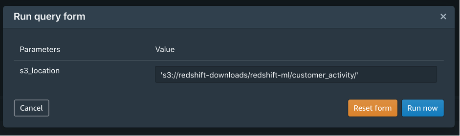
You would probably like to reuse the load query in the future to load data in from another S3 location. In that case, you can use the parameterized query by replacing the S3 URL of the as shown in the following screenshot:

SavingQ2

You can save the query, and then share the query with another user.

When you or other users run the query, a prompt for the parameter will appear as in the following screenshot:

SavingQ3

We discussed how data analysts could load data into their own or the group’s workspace.

We will now discuss using Query Editor V2 to create an external schema to extend your data warehouse to the data lake.

Extending the Data Warehouse to the Data Lake

Extending Data warehouses to Data lakes is part of modern data architecture practices. Amazon Redshift enables this with seamless integration through Data lake running on AWS. Redshift uses Spectrum to allow this extension. You can access data lakes from the Redshift Data warehouse by creating Redshift external schemas.

Query Editor V2 lets you create an external schema referencing an external database in AWS Glue Data Catalogue.

To extend your Data Warehouse to Data Lake, you should have an S3 data lake and AWS Glue Data Catalog database defined for the data lake. Grant permission on AWS Glue to Redshift Cluster Role. You can find more information about external Schema here.

You can navigate to the Create External Schema by using Create Schema wizard, and then selecting the External Schema as shown in the following screenshot:

The Query Editor V2 makes the schema creation experience very easy by hiding the intricacies of the create external schema syntax. You can use the simple interface and provide the required parameters, such as Glue data regions, external database name, and the IAM role. You can browse the Glue Catalog and view the database name.

After you use the create schema option, you can see the schemas in the tree-view. The Query Editor V2 uses distinct icons to distinguish between native Schema and external Schema.

Viewing External Table Definitions

The Query Editor V2 lets data analysts quickly view objects available in external databases and understand their metadata.

You can view tables and columns for a given table by clicking on external Schema and then on a table. When a particular table is selected, its metadata information is displayed in the bottom portion below the tree-view panel. This is a powerful feature, as an analyst can easily understand the data residing externally in the data lake.

You can now run queries against external tables in the external Schema.

In our fictitious enterprise, Marketing Department team members can load data in their own workspace and join the data from their own user/group workspace with the curated data in the enterprise data warehouse or data lake.

Conclusion

This post demonstrated how the Query Editor V2 enabled data analysts to create tables and load data from Amazon S3 easily with a simple wizard.

We also discussed how Query Editor V2 lets you extend the data warehouse to a data lake. The data analysts can easily browse tables in your local data warehouse, data shared from another cluster, or tables in the data lake. You can run queries that can join tables in your data warehouse and data lake. The Query Editor V2 also provides several features for the collaboration of query authoring. You can view the earlier blog to learn more about how the Query Editor V2 simplifies data analysis.

These features let organizations accelerate self-service analytics and end-users deliver the insights faster.

Happy querying!

About the Authors

Bhanu Pittampally is Analytics Specialist Solutions Architect based out of Dallas. He specializes in building analytical solutions. His background is in data warehouse – architecture, development and administration. He is in data and analytical field for over 13 years. His Linkedin profile is here.

Debu Panda is a Principal Product Manager at AWS, is an industry leader in analytics, application platform, and database technologies, and has more than 25 years of experience in the IT world.

Cansu Aksu is a Front End Engineer at AWS, has a several years of experience in developing user interfaces. She is detail oriented, eager to learn and passionate about delivering products and features that solve customer needs and problems

Chengyang Wang is a Frontend Engineer in Redshift Console Team. He worked on a number of new features delivered by redshift in the past 2 years. He thrives to deliver high quality products and aim to improve customer experience from UI

Performance Improvements

Optimizing with table-level statistics

Improvements with AWS Glue Data Catalog column statistics

Query rewrite optimization

Bloom filter for partition columns

Conclusion

About the authors

Solution overview

Prerequisites

Automatically mount access grants to the Amazon DataZone environment role

Query using Redshift Spectrum

Aggregate tables and unify products

Clean up

Conclusion

About the Authors

Overview of solution

Dataset

Create the offline feature group and ingest data

Create a Redshift table and load local feature data

Create an external schema for Redshift Spectrum to access the offline store data

Train and validate the fraud risk scoring ML model

Use the offline feature store and local store for inference

Clean up

Conclusion

About the authors

Solution overview

Prerequisites

Archival and purging

Schedule the stored procedure

Archive data in Amazon S3

Analyze the archived data in Amazon S3 using Amazon Redshift Spectrum

Best practices

Conclusion

About the authors

The Goal to Accelerate and Empower Data Analysts

An example Use case

Prerequisites

Create Schemas

Creating Tables

Loading Data

Viewing load errors

Saving and reusing the queries

Extending the Data Warehouse to the Data Lake

Viewing External Table Definitions

Conclusion

About the Authors

The collective thoughts of the interwebz