Post Syndicated from Ying Wang original https://aws.amazon.com/blogs/big-data/talk-to-your-data-query-your-data-lake-with-amazon-quicksight-q/
Amazon QuickSight Q uses machine learning (ML) and natural language technology to empower you to ask business questions about your data and get answers instantly. You can simply enter your questions (for example, “What is the year-over-year sales trend?”) and get the answer in seconds in the form of a QuickSight visual.
Some business questions can’t be answered through existing business intelligence (BI) dashboards. It can take days or weeks for the BI team to accommodate these needs and refine their solution. Because Q doesn’t depend on prebuilt dashboards or reports to answer questions, it removes the need for BI teams to create or update dashboards every time a new business question arises. You can ask questions and receive answers in the form of visuals in seconds directly from within QuickSight or from web applications and portals. Q empowers every business user to self-serve and get insights faster, regardless of their background or skillset.
In this post, we walk you through the steps to configure Q using an Olympic Games public dataset and demonstrate how an end-user can ask simple questions directly from Q in an interactive manner and receive answers in seconds.
You can interactively play with the Olympic dashboard and Q search bar in the following interactive demo.

Solution overview
We use Olympic games public datasets to configure a Q topic and discuss tips and tricks on how to make further configurations on the topic that enable Q to provide prompt answers using ML-powered, natural language query (NLQ) capabilities that empower you to ask questions about data using everyday business language.
The video from Data Con LA provides a high-level demonstration of the capabilities covered in this post.
Additionally, we discuss the following:
- Best practices for data modeling of a Q topic
- How to perform data cleansing using AWS Glue DataBrew, SQL, or an Amazon SageMaker Jupyter notebook on datasets to build a Q topic
We use multiple publicly available datasets from Kaggle. The datasets have historical information about athletes, including name, ID, age, weight, country, and medals.
We use the 2020 Olympic datasets and historical data. We also use the datasets Introduction of Women Olympic Sport and Women of Olympic Games to determine the participation of women athletes in Olympics and discover trends. The QuickSight datasets created using these public data files are added to a Q topic, as shown in the following screenshot. We provide details on creating QuickSight datasets later in this post.

Prerequisites
To follow along with the solution presented in this post, you must have access to the following:
Create solution resources
The public datasets in Kaggle can’t be directly utilized to create a Q topic. We have already cleansed the raw data and have provided the cleansed datasets in the GitHub repo. If you are interested in learning more about data cleansing, we discussed three different data cleansing methods at the end of this post.
To create your resources, complete the following steps:
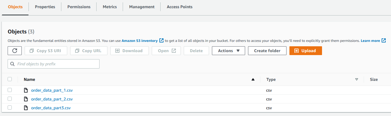
- Create an S3 bucket called
olympicsdata. - Create a folder for each data file, as shown in the following screenshot.

- Upload the data files from the GitHub repo into their respective folders.
- Deploy the provided CloudFormation template and provide the necessary information.

The template creates an Athena database and tables, as shown in the following screenshot.

The template also creates the QuickSight data source athena-olympics and datasets.

Create datasets in QuickSight
To build the Q topic, we need to combine the datasets, because each table contains only partial data. Joining these tables helps answer questions across all the features of the 2020 Olympics.
We create the Olympics 2021 dataset by joining the tables Medals_athletes_2021, Athletes_full_2021, Coach_full_2021, and Tech_official_2021.
The following screenshot shows the joins for our complete dataset.

Medals_athletes_2021 is the main table, with the following join conditions:
- Left outer join
athletes_full_2021onathlete_name,discipline_code, andcountry_code - Left outer join
coach_full_2021on country, discipline, and event - Left outer join
tech_official_2021on discipline
Finally, we have the following datasets that we use for our Q topic:
- Olympics 2021 Details
- Medals 2021
- Olympics History (created using the
Olympicstable) - Introduction of Women Olympics Sports
- Women in the Olympic Movement
Create a Q topic
Topics are collections of one or more datasets that represent a subject area that your business users can ask questions about. In QuickSight, you can create and manage topics on the Topics page. When you create a topic, your business users can ask questions about it in the Q search bar.
When you create topics in Q, you can add multiple datasets to them and then configure all the fields in the datasets to make them natural language-friendly. This enables Q to provide your business users with the correct visualizations and answers to their questions.
The following are data modeling best practices for Q topics:
- Reduce the number of datasets by consolidating the data. Any given question can only hit one data set, so only include multiple datasets if they are related enough to be part of the same topic, but distinct enough that you can ask a question against them independently.
- For naming conventions, provide a meaningful name or alias (synonym) of a field to allow the end-user to easily query it.
- If a field appears in different datasets, make sure that this field has the same name across different datasets.
- Validate data consistency. For example, the total value of a metric that aggregates from different datasets should be consistent.
- For fields that don’t request on-the-fly calculations, for example, metrics with distributive functions (sum, max, min, and so on), push down the calculation into a data warehouse.
- For fields that request on-the-fly calculations, create the calculated field in the QuickSight dataset or Q topic. If other topics or dashboards might reuse the same field, create it in the datasets.
To create a topic, complete the following steps:
- On the QuickSight console, choose Topics in the navigation pane.
- Choose New topic.

- For Topic name, enter a name.
- For Description, enter a description.
- Choose Save.

- On the Add data to topic page that opens, choose Datasets, and then select the datasets that we created in the previous section.
- Choose Add data to create the topic.


Enhance the topic
In this section, we discuss various ways that you can enhance the topic.
Add calculated fields to a topic dataset
You can add new fields to a dataset in a topic by creating calculated fields.
For example, we have the column Age in our Olympics dataset. We can create a calculated field to group age into different ranges using the ifelse function. This calculated field can help us ask a question like “How many athletes for each age group?”
- Choose Add calculated field.
- In the calculation editor, enter the following syntax:
- Name the calculated field
Age Groups. - Choose Save.
The calculated field is added to the list of fields in the topic.
Add filters to a topic dataset
Let’s say lot of analysis is expected on the dataset for the summer season. We can add a filter to allow for easy selection of this value. Furthermore, if we want to allow analysis against data for the summer season only, we can choose to always apply this filter or apply it as the default choice, but allow users to ask questions about other seasons as well.
- Choose Add filter.
- For Name, enter
Summer. - Choose the
Women in the Olympic Movementdataset. - Choose the
Olympics Seasonfield. - Choose Custom filter list for Filter type and set the rule as include.
- Enter Summer under Values.
- Choose Apply always, unless a question results in an explicit filter from the dataset.
- Choose Save.
The filter is added to the list of fields in the topic.
Add named entities to a topic dataset
We can define named entities if we need to show users a combination of fields. For example, when someone asks for player details, it makes sense to show them player name, age, country, sport, and medal. We can make this happen by defining a named entity.
- Choose Add named entity.
- Choose the
Olympicsdataset. - Enter
Player Profilefor Name. - Enter
Information of Playerfor Description. - Choose Add field.
- Choose Player Name from the list.
- Choose Add field again and add the fields
Age,Countries,Sport, andMedal.
The fields listed are the order they appear in answers. To move a field, choose the six dots next to the name and drag and drop the field to the order that you want. - Choose Save.
The named entity is added to the list of fields in the topic.
Make Q topics natural language-friendly
To help Q interpret your data and better answer your readers’ questions, provide as much information about your datasets and their associated fields as possible.
To make the topic more natural language-friendly, use the following procedures.
Rename fields
You can make your field names more user-friendly in your topics by renaming them and adding descriptions.
Q uses field names to understand the fields and link them to terms in your readers’ questions. When your field names are user-friendly, it’s easier for Q to draw links between the data and a reader’s question. These friendly names are also presented to readers as part of the answer to their question to provide additional context.
Let’s rename the birth date field from the athlete dataset as Athlete Birth Date. Because we have multiple birth date fields in the topics for coach, athlete, and tech roles, renaming the athletes’ birth date field helps Q easily link to the data field when we ask questions regarding athletes’ birth dates.
- On the Fields page, choose the down arrow at far right of the
Birth Datefield to expand it. - Choose the pencil icon next to the field name.
- Rename the field to
Athlete Birth Date.

Add synonyms to fields in a topic
Even if you update your field names to be user-friendly and provide a description for them, your readers might still use different names to refer to them. For example, a player name field might be referred to as player, players, or sportsman in your reader’s questions.
To help Q make sense of these terms and map them to the correct fields, you can add one or more synonyms to your fields. Doing this improves Q’s accuracy.
- On the Fields page, under Synonyms, choose the pencil icon for
Player Name. - Enter
playerandsportsmanas synonyms.
Add synonyms to field values
Like we did for field names, we can add synonyms for category values as well.
- Choose the
Genderfield’s row to expand it. - Choose Configure value synonyms, then choose Add.
- Choose the pencil icon next to the F value.
- Add the synonym
Female. - Repeat these steps to add the synonym
MaleforM. - Choose Done.

Assign field roles
Every field in your dataset is either a dimension or a measure. Knowing whether a field is a dimension or a measure determines what operations Q can and can’t perform on a field.
For example, setting the field Age as a dimension means that Q doesn’t try to aggregate it as it does measures.
- On the Fields page, expand the Age field.
- For Role, choose Dimension.

Set field aggregations
Setting field aggregations tells Q which function should or shouldn’t be used when those fields are aggregated across multiple rows. You can set a default aggregation for a field, and specify aggregations that aren’t allowed.
A default aggregation is the aggregation that’s applied when there’s no explicit aggregation function mentioned or identified in a reader’s question. For example, let’s ask Q “Show total number of events.” In this case, Q uses the field Total Events, which has a default aggregation of Sum, to answer the question.
- On the Fields page, expand the Total Events field.
- For Default aggregation, choose Sum.
- For Not allowed aggregation, choose Average.

Specify field semantic types
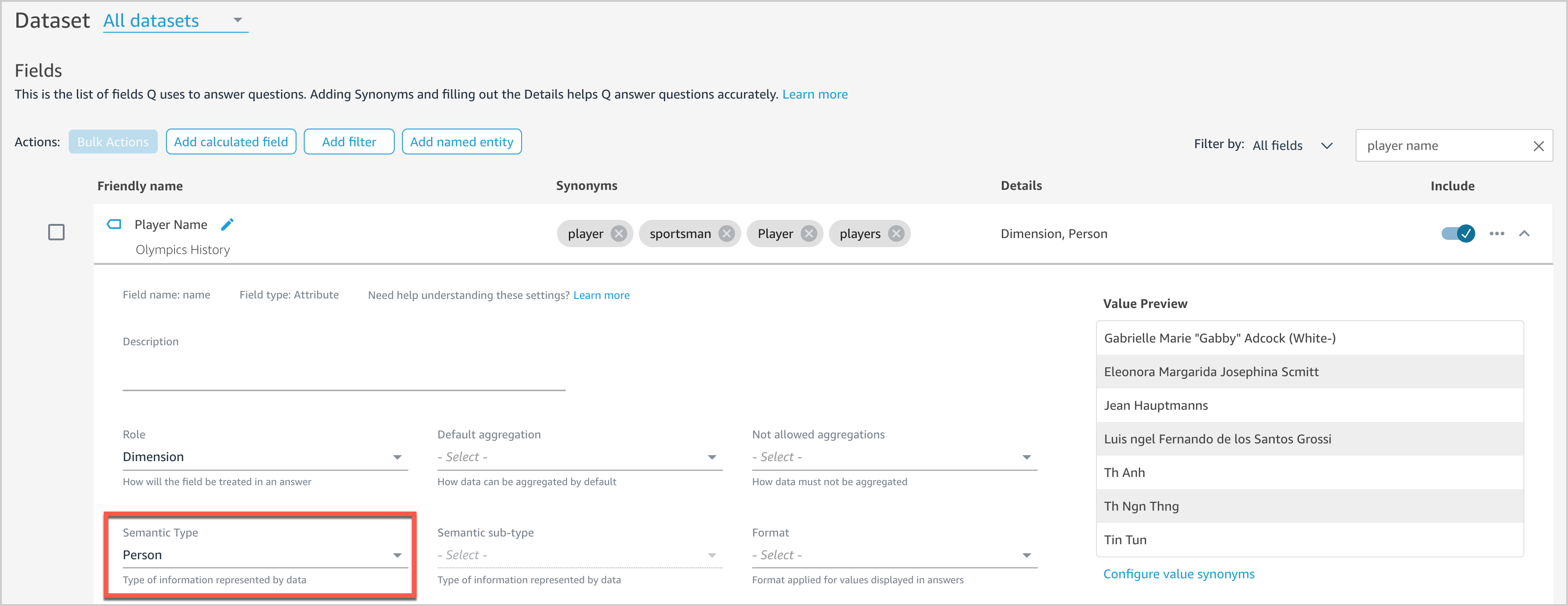
Providing more details on the field context will help Q answer more natural language questions. For example, users might ask “Who won the most medals?” We haven’t set any semantic information for any fields in our dataset yet, so Q doesn’t know what fields to associate with “who.” Let’s see how we can enable Q to tackle this question.
- On the Fields page, expand the
Player Namefield. - For Semantic Type, choose Person.
This enables Q to surface Player Name as an option when answering “who”-based questions.
Exclude unused or unnecessary fields
Fields from all included datasets are displayed by default. However, we have a few fields like Short name of Country, URL Coach Full 2021, and URL Tech Official 2021 that we don’t need in our topic. We can exclude unnecessary fields from the topic to prevent them from showing up in results by choosing the slider next to each field.

Ask questions with Q
After we create and configure our topic, we can now interact with Q by entering questions in the Q search bar.
For example, let’s enter show total medals by country. Q presents an answer to your question as a visual.
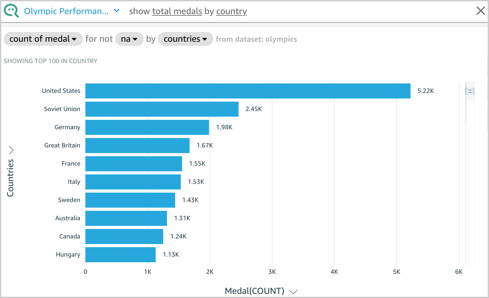
You can see how Q interpreted your question in the description at the visual’s upper left. Here you can see the fields, aggregations, topic filters, and datasets used to answer the question. The topic filter na is applied on the Medal attribute, which excludes na values from the aggregation. For more information on topic filters, see Adding filters to a topic dataset.

Q displays the results using the visual type best suited to convey the information. However, Q also gives you the flexibility to view results in other visual types by choosing the Visual icon.
Another example, let’s enter who is the oldest player in basketball. Q presents an answer to your question as a visual.

Sometimes Q might not interpret your question the way you wanted. When this happens, you can provide feedback on the answer or make suggestions for corrections to the answer. For more information about providing answer feedback, see Providing feedback about QuickSight Q topics. For more information about correcting answers, see Correcting wrong answers provided by Amazon QuickSight Q.
Conclusion
In this post, we showed you how to configure Q using an Olympic games public dataset and so end-users can ask simple questions directly from Q in an interactive manner and receive answers in seconds. If you have any feedback or questions, please leave them in the comments section.
Appendix 1: Types of questions supported by Q
Let’s look at samples of each question type that Q can answer using the topic created earlier in this post.
Try the following questions or your own questions and continue enhancing the topic to improve accuracy of responses.
| Question Type | Example |
| Dimensional Group Bys | show total medals by country |
| Dimensional Filters (Include) | show total medals for united states |
| Date Group Bys | show yearly trend of women participants |
| Multi Metrics | number of women events compared to total events |
| KPI-Based Period over Periods (PoPs) | how many women participants in 2018 over 2016 |
| Relative Date Filters | show total medals for united states in the last 5 years |
| Time Range Filters | list of women sports introduced since 2016 |
| Top/Bottom Filter | show me the top 3 player with gold medal |
| Sort Order | show top 3 countries with maximum medals |
| Aggregate Metrics Filter | show teams that won more than 50 medals |
| List Questions | list the women sports by year in which they are introduced |
| OR filters | Show player who got gold or silver medal |
| Percent of Total | Percentage of players by country |
| Where Questions | where are the most number of medals |
| When Questions | when women volleyball introduced into olympic games |
| Who Questions | who is the oldest player in basketball |
| Exclude Questions | show countries with highest medals excluding united states |
Appendix 2: Data cleansing
In this section, we provide three options for data cleansing: SQL, DataBrew, and Python.
Option 1: SQL
For our first option, we discuss how to create Athena tables on the downloaded Excel or CSV files and then perform the data cleansing using SQL. This option is suitable for those who use Athena tables as a data source for QuickSight datasets and are comfortable using SQL.
The SQL queries to create Athena tables are available in the GitHub repo. In these queries, we perform data cleansing by renaming, changing the data type of some columns, as well as removing the duplicates of rows. Proper naming conventions and accurate data types help Q efficiently link the questions to the data fields and provide accurate answers.
Use the following sample DDL query to create an Athena table for women_introduction_to_olympics:
In our data files, there are few columns that are common across more than one dataset that have different column names. For example, gender is available as gender or sex, country is available as country or team or team/noc, and person names have a role prefix in one dataset but not in other datasets. We rename such columns using SQL to maintain consistent column names.
Additionally, we need to change other demographic columns like age, height, and weight to the INT data type, so that they don’t get imported as String.
The following columns from the data files have been transformed using SQL.
| Data File | Original Column | New Column |
| medals | DisciplineMedal_date (timestamp) |
SportMedal_date (date) |
| Athletes | namegenderbirth_datebirth_placebirth_country |
athlete_nameathlete_genderathlete_birth_dateathlete_birth_placeathlete_birth_country |
| Coaches | namegenderbirth_datefunction |
coach_namecoach_gendercoach_birth_datecoach_function |
| Athlete_events (history) | TeamNOCAge (String)Height (String)Weight (String) |
countrycountry_codeAge (Integer)Height (Integer)Weight (Integer) |
Option 2: DataBrew
In this section, we discuss a data cleansing option using DataBrew. DataBrew is a visual data preparation tool that makes it easy to clean and prepare data with no prior coding knowledge. You can directly load the results into an S3 bucket or load the data by uploading an Excel or CSV file.
For our example, we walk you through the steps to implement data cleansing on the medals_athletes_2021 dataset. You can follow the same process to perform any necessary data cleaning on other datasets as well.
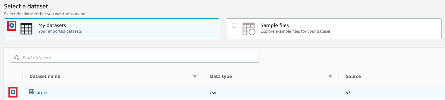
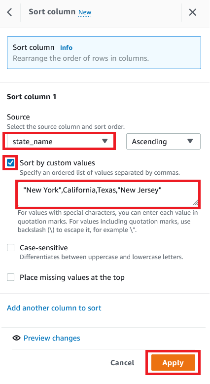
Create a new dataset in DataBrew using medals_athletes.csv and then create a DataBrew project and implement the following recipes to cleanse the data in the medals_athletes_2021 dataset.
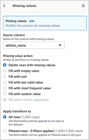
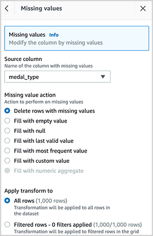
- Delete empty rows in the
athlete_namecolumn.

- Delete empty rows in the
medal_typecolumn.

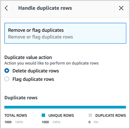
- Delete duplicate rows in the dataset.

- Rename discipline to
Sport.

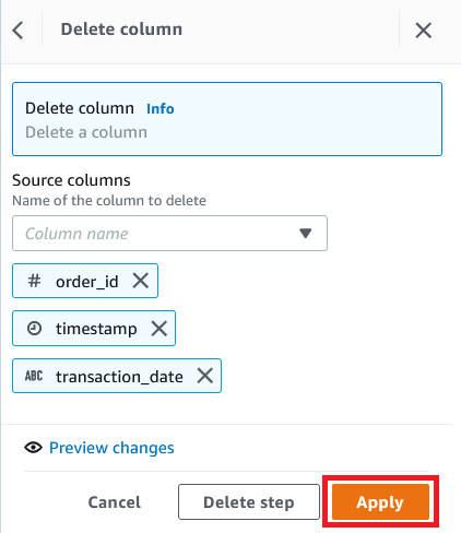
- Delete the column
discipline_code.

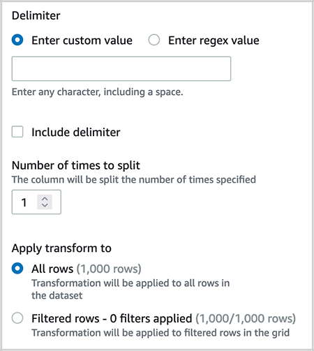
- Split the column
medal_typeon a single delimiter.

- Delete the column
medal_type_2, which was created as a result of step 6.

- Rename
medal_type_1tomedal_type.

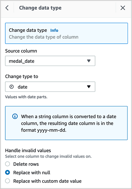
- Change the data type of column
medal_datefrom timestamp to date.


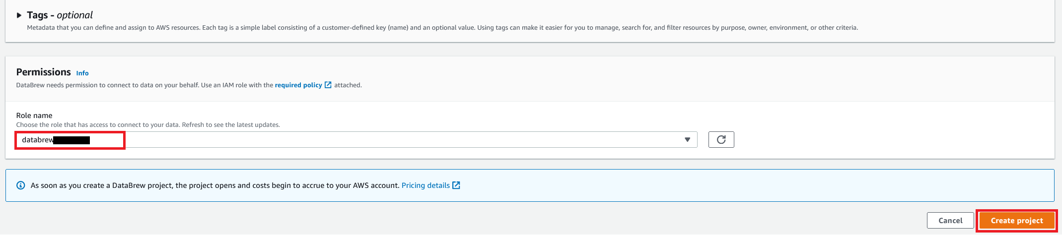
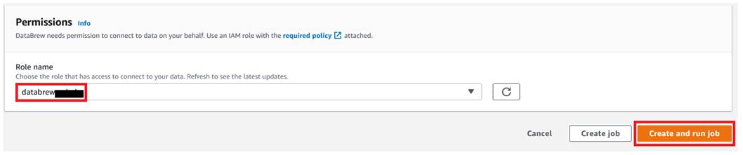
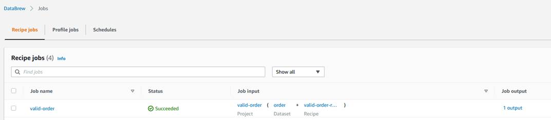
After you create the recipe, publish it and create a job to output the results in your desired destination. You can create QuickSight SPICE datasets by importing the cleaned CSV file.
Option 3: Python
In this section, we discuss data cleansing using NumPy and Pandas of Python on the medals_athletes_2021 dataset. You can follow the same process to perform any necessary data cleansing on other datasets as well. The sample Python code is available on GitHub. This option is suitable for someone who is comfortable processing the data using Python.
- Delete the column
discipline_code: - Rename the column discipline to sport:
You can create QuickSight SPICE datasets by importing the cleansed CSV.
Appendix 3: Data cleansing and modeling in the QuickSight data preparation layer
In this section, we discuss one more method of data cleansing that you can perform from the QuickSight data preparation layer, in addition to the methods discussed previously. Using SQL, DataBrew, or Python have advantages because you can prepare and clean the data outside QuickSight so other AWS services can use the cleansed results. Additionally, you can automate the scripts. However, Q authors have to learn other tools and programming languages to take advantage of these options.
Cleansing data in the QuickSight dataset preparation stage allows non-technical Q authors to build the application end to end in QuickSight with a codeless method.
The QuickSight dataset stores any data preparation done on the data, so that the prepared data can be reused in multiple analyses and topics.
We have provided a few examples for data cleansing in the QuickSight data preparation layer.
Change a field name
Let’s change the name data field from Athletes_full_2021 to athlete_name.
- In the data preview pane, choose the edit icon on the field that you want to change.
- For Name, enter a new name.
- Choose Apply.


Change a field data type
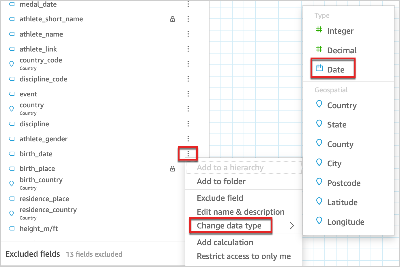
You can change the data type of any field from the data source in the QuickSight data preparation layer using the following procedure.
- In the data preview pane, choose the edit icon on the field you want to change (for example,
birth_date). - Choose Change data type and choose Date.
This converts the string field to a date field.
Appendix 4: Information about the tables
The following table illustrates the scope of each table in the dataset.
| Table Name | Link | Table Data Scope |
medals |
https://www.kaggle.com/piterfm/tokyo-2020-olympics?select=medals.csv | Information about medals won by each athlete and the corresponding event and country details |
athletes |
https://www.kaggle.com/piterfm/tokyo-2020-olympics?select=athletes.csv | Details about each athlete, such as demographic and country |
coaches |
https://www.kaggle.com/piterfm/tokyo-2020-olympics?select=coaches.csv | Details about each coach, such as demographic and country |
technical_officials |
https://www.kaggle.com/piterfm/tokyo-2020-olympics?select=technical_officials.csv | Details about each technical official, such as demographic and country |
athlete_events |
https://www.kaggle.com/heesoo37/120-years-of-olympic-history-athletes-and-results | Historical information of Olympic games |
Introduction_of_Women_Olympics_Sports |
https://data.world/sports/women-in-the-olympic-games | Information on when the women Olympic sports were introduced |
womens_participation_in_the_olympic |
https://data.world/sports/women-in-the-olympic-games | Information on participation of women in Olympic sports |
About the authors
 Ying Wang is a Manager of Software Development Engineer. She has 12 years experience in data analytics and data science. In her data architect life, she helped customer on enterprise data architecture solutions to scale their data analytics in the cloud. Currently, she helps customer to unlock the power of Data with QuickSight from engineering/product by delivering new features.
 Ginni Malik is a Data & ML Engineer with AWS Professional Services. She assists customers by architecting enterprise level data lake solutions to scale their data analytics in the cloud. She is a travel enthusiast and likes to run half-marathons.
 Niharika Katnapally is a QuickSight Business Intelligence Engineer with AWS Professional Services. She assists customers by developing QuickSight dashboards to help them gain insights into their data and make data driven business decisions.


 Jack Mazanec is a software engineer working on OpenSearch plugins. His primary interests include machine learning and search engines. Outside of work, he enjoys skiing and watching sports.
 Othmane Hamzaoui is a Data Scientist working at AWS. He is passionate about solving customer challenges using Machine Learning, with a focus on bridging the gap between research and business to achieve impactful outcomes. In his spare time, he enjoys running and discovering new coffee shops in the beautiful city of Paris.


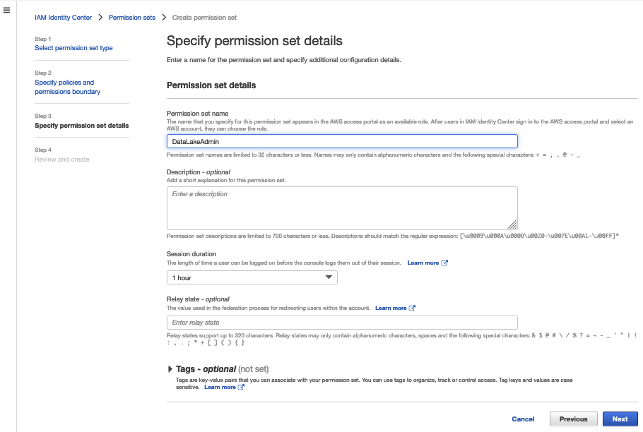


 Under Map Attributes, there should be four attributes.


 On the Attribute Mappings tab, you now add or update the attributes as in the following table.
 Srikanth Baheti is a Specialized World Wide Sr. Solution Architect for Amazon QuickSight. He started his career as a consultant and worked for multiple private and government organizations. Later he worked for PerkinElmer Health and Sciences & eResearch Technology Inc, where he was responsible for designing and developing high traffic web applications, highly scalable and maintainable data pipelines for reporting platforms using AWS services and Serverless computing.
 Raji Sivasubramaniam is a Sr. Solutions Architect at AWS, focusing on Analytics. Raji is specialized in architecting end-to-end Enterprise Data Management, Business Intelligence and Analytics solutions for Fortune 500 and Fortune 100 companies across the globe. She has in-depth experience in integrated healthcare data and analytics with wide variety of healthcare datasets including managed market, physician targeting and patient analytics.
 Raj Jayaraman is a Senior Specialist Solutions Architect for Amazon QuickSight. Raj focuses on helping customers develop sample dashboards, embed analytics and adopt BI design patterns and best practices.
 Sindhu Chandra is a Senior Product Marketing Manager for Amazon QuickSight, AWS’ cloud-native, business intelligence (BI) service that delivers easy-to-understand insights to anyone, wherever they are.