Tag Archives: Analytics

Doing data preparation using on-premises PostgreSQL databases with AWS Glue DataBrew

Post Syndicated from John Espenhahn original https://aws.amazon.com/blogs/big-data/doing-data-preparation-using-on-premises-postgresql-databases-with-aws-glue-databrew/

Today, with AWS Glue DataBrew, data analysts and data scientists can easily access and visually explore any amount of data across their organization directly from their Amazon Simple Storage Service (Amazon S3) data lake, Amazon Redshift data warehouse, and Amazon Aurora and Amazon Relational Database Service (Amazon RDS) databases. Customers can choose from over 250 built-in functions to combine, pivot, and transpose the data without writing code.

Now, with added support for JDBC-accessible databases, DataBrew also supports additional data stores including PostgreSQL, MySQL, Oracle, and Microsoft SQL Server. In this blog post, we will be using DataBrew to clean data from an on-premise database, and storing the cleaned data in an Amazon S3 data lake.

Solution Overview

I will be configuring an existing subnet in an Amazon VPC for use with DataBrew. Then configuring DataBrew to securely connect to an existing on-premise database and executing a data preparation job.

Components

  1. You should have an AWS account with a Virtual Private Cloud (Amazon VPC). DataBrew will connect to your database from this VPC.
  2. You should have a subnet within your Amazon VPC. In this blog, this subnet will be configured for use with DataBrew.
  3. You should have an on-premise database with data to be cleaned with DataBrew.
  4. I assume you have a VPN connection between your Amazon VPC and on premise network to enable secure connections between them. I’ve implemented a VPN tunnel using AWS Site-to-Site VPN. You may choose to  Simulate Site-to-Site VPN Customer Gateways Using strongSwan.
  5. This guide will walk through creation of a DataBrew dataset, project, and job.
  6. DataBrew requires access to Amazon S3 and AWS Glue. This guide will walk through creating VPC endpoints to enable private connections between your VPC and these AWS services for DataBrew to use.
  7. To establish network connectivity, DataBrew will provision an Amazon VPC elastic network interface in the VPC you specify. This blog will cover securing this network interface with a security group.

Prerequisites

To complete this blog, you should have the following prerequisites:

Additionally, you will need to have enabled access to your on-premise network from the subnet in the Amazon VPC. If you haven’t enabled it already, you can Simulate Site-to-Site VPN Customer Gateways Using strongSwan, or you can enable access by completing the AWS Site-to-Site VPN getting started guide.

If you are unsure if you have enabled access from your VPC subnet to your on-premise database, you can test access by running the AWS Systems Manager automation AWSSupport-SetupIPMonitoringFromVPC. From the User Guide, choose Run this Automation. In the Systems Manager console, under Input Parameters, you will need to enter the Amazon VPC subnet ID for SubnetId and the IP address of your on-premise host for TargetIPs. Then choose Execute. Once the automation completes, locate the Outputs section and open the URL linked under createCloudWatchDashboard.Output. From that dashboard, confirm from the Ping log group that pings are successful. If they are not, you will need to investigate. A useful resource for this is How do I troubleshoot instance connection timeout errors in Amazon VPC.

Step 1: Configure the Amazon VPC

Ensure your Amazon VPC has DNS Support and DNS Hostnames enabled. You can verify this by selecting your VPC in the Amazon VPC console and checking the details for DNS hostnames and DNS resolution. If they are disabled, they can be enabled by choosing Actions then the corresponding Edit option.

On-premise or hybrid DNS are also supported, but requires additional setup. See Other Considerations at the end of this post for more.

Step 2: Configure the Amazon VPC Subnet

Your subnet must have access to Amazon S3 and AWS Glue services. I will add VPC endpoints for Amazon S3 and AWS Glue services to keep my traffic within the AWS network.

  1. To add the VPC endpoint for Amazon S3, open the Amazon VPC console at https://console.aws.amazon.com/vpc/.
  2. In the navigation pane, choose Endpoints, Create Endpoint.
  3. Filter by “s3”.
  4. Choose the service where the Type column indicates Gateway.
  5. Select the route tables associated with the subnet to be used with DataBrew.
  6. Choose Create endpoint.
  7. To add the VPC endpoint for AWS Glue, again choose Create Endpoint.
  8. Filter by “glue”.
  9. Choose the service where the Type column indicates Interface.
  10. Select the route tables associated with the subnet to be used with DataBrew.
  11. Choose Create endpoint.

Step 3 : Configure Network ACL

By default Network ACLs allow all inbound and outbound traffic. If you have customized your network ACL, ensure inbound return traffic from and outbound traffic to your on-premise network, Amazon S3, and AWS Glue are allowed.

  1. From the Amazon VPC console, choose Subnets.
  2. Choose the subnet you are using with DataBrew.
  3. From the Details tab, choose the Network ACL link.
  4. Validate your inbound and outbound rules, updating your rules to allow the required traffic if needed. The screenshot below shows the default rules I am using.

Step 4: Configure the VPC security group

To provide connectivity to your VPC, DataBrew will create an Elastic Network Interface (ENI) in the VPC subnet you specify. DataBrew attaches the security group you specify to the ENI to limit network access. This security group must have a self-referential rule to allow all inbound TCP traffic from itself. This will block access from unspecified sources. I will be using the default security group, which has the following configuration.

Your security group must allow outbound traffic to itself, Amazon S3, AWS Glue, and your on-premise network. I’ll be using the default security group, which allows all outbound traffic.

Optionally, you may wish to explicitly restrict outbound traffic to only your on-premise network, Amazon S3, and AWS Glue. To do so, remove the All TPC outbound rule. Ensure your security group has a self-referential rule to allow all outbound TCP traffic to itself. Allow traffic to your on-premise network by specifying the CIDR block associated with your network. In my case, it is 10.196.0.0/16. Allow traffic to Amazon S3 with the AWS-managed S3 prefix list, which includes the set of CIDR blocks for Amazon S3. Allow traffic to the AWS Glue VPC endpoint by associating the same security group with the AWS Glue VPC endpoint created above from the Amazon VPC console.

An example of what these scoped-down outbound rules may look like:

Ensure your on-premise network security rules allow traffic from your Amazon VPC subnet’s CIDR block.

Step 5 : Create database credentials

Following best practices, I will be creating a database user with scoped down permissions for use with DataBrew.

  1. Connect to your database. In my case with psql -h 10.196.0.20
  2. Create a user, which I’ll call postgresql, with readonly access to the table that will be used with DataBrew. My table is called demo in database postgres. I’ll do this by executing the following queries:
    CREATE USER postgresql WITH PASSWORD ‘****’;
    GRANT CONNECT ON DATABASE postgres TO postgresql;
    GRANT USAGE ON SCHEMA public TO postgresql;
    REVOKE CREATE ON SCHEMA public FROM postgresql;
    GRANT SELECT ON demo TO postgresql;

Step 6 : Create DataBrew project

  1. From the AWS DataBrew console, choose Create project.
  2. Enter a Project name.
  3. Under Select a dataset choose New dataset.
  4. Enter a Dataset name.
  5. Under Connect to new dataset choose JDBC.
  6. Choose Add JDBC connection.
  7. Enter a Connection name, I use my-connection.
  8. Choose Enter JDBC details.
  9. Choose Database type, in my case PostgreSQL.
  10. For Host/endpoint, enter your host’s private IP address.
  11. Enter your Database name, Database user, and Database password.
  12. Choose your VPC, and the Subnet and Security Group you configured above.
  13. Review “Additional configurations”, where you can optionally configure the following:

    1. If you are using a recent database version, such as MySQL 8, you may need to provide a custom JDBC driver. For more information, see the Developer Guide.
    2. DataBrew can be set to fail the connection to your database if it is unable to connect over SSL. Additionally, DataBrew provides default certificates for establishing SSL connections. If you obtained a certificate from a third-party issuer, or the default certificates provided by DataBrew do not meet your requirements, you can provide your own. DataBrew handles only X.509 certificates. The certificate must be DER-encoded and supplied in base64 encoding PEM format.
  14. Choose Create connection at the bottom of the modal.
  15. Choose the newly created connection by clicking on its name.
  16. Enter the name of the table within your database you want to bring into DataBrew.
  17. Under the Permissions header, choose Create new IAM role from the dropdown and enter a role suffix.
  18. Choose Create project, this will open the project view. After one to two minutes you will be able to work with your data. If the connection fails, see How do I troubleshoot instance connection timeout errors in Amazon VPC.
  19. Start by applying some simple transforms, I’m dropping some columns that are not needed in my data lake. To do so, from the action bar I choose COLUMN, then Delete.
  20. This opens the side-bar where I choose the column to delete, and choose Apply.

Step 7 : Create DataBrew job

Once I’ve got a few transforms added to my project’s recipe, I will run a job to execute the recipe against my full dataset, and store the result in my Amazon S3 bucket.

  1. Choose Create job from the top of the project grid view.
  2. On the job page, provide a Job name and S3 output location.
  3. Under the header Permissions, choose Create new IAM role. This will create a new scoped down IAM role with the permissions required to execute your job.
  4. Finally, choose Create and run job. Once the job completes, you can view the output in Amazon S3.

Cleanup

From the DataBrew console, delete your Job, Project, Recipe, and Dataset.

If you executed the Systems Manager automation to test access, under the Systems Manager console, choose CloudWatch Dashboard. Select the dashboard created by the automation. Choose Terminate test. Then choose Execute.

Other considerations

AWS Glue DataBrew’s networking requirements are similar to that of AWS Glue ETL jobs. Below summarizes some of those advanced networking conditions. For more details on AWS Glue ETL, see How to access and analyze on-premises data stores using AWS Glue by Rajeev Meharwal.

DNS

If you are using AWS VPC provided DNS, ensure you have enabled DnsHostnames and DnsSupport for your VPC. For more information, see DNS support in your VPC.

If you have configured a custom DNS server with your AWS VPC, you must implement forward and reverse lookups for Amazon EC2 private DNS hostnames. For more information, see Amazon DNS server. Alternatively, setup hybrid DNS resolution to resolve both on-premise DNS servers and the VPC provided DNS. For implementation details, see the following AWS Security Blog posts:

Joining or unioning multiple databases

If you are joining a database dataset into your project, the database must be accessible from the project dataset’s subnet.

For example, if you have completed the setup above using Private Subnet 1, and you have another Amazon RDS database in Private Subnet 2 in the same VPC, as shown below. You will want a local route for the route table associated with Subnet 1. You will also need to ensure the security group attached to your Amazon RDS database allows inbound traffic from your DataBrew security group.

If your Amazon RDS database is in a different AWS VPC than you are using with DataBrew, you will need to setup VPC peering.


About the Authors

John Espenhahn is a Software Engineer working on AWS Glue DataBrew service. He has also worked on Amazon Kendra user experience as a part of Database, Analytics & AI AWS consoles. He is passionate about technology and building in the analytics space.


Nitya Sheth is a Software Engineer working on AWS Glue DataBrew service. He has also worked on AWS Synthetics service as well as on user experience implementations for Database, Analytics & AI AWS consoles. In his free time, he divides his time between exploring new hiking places and new books.


Simplify semi-structured nested JSON data analysis with AWS Glue DataBrew and Amazon QuickSight

Post Syndicated from Sriharsh Adari original https://aws.amazon.com/blogs/big-data/simplify-semi-structured-nested-json-data-analysis-with-aws-glue-databrew-and-amazon-quicksight/

As the industry grows with more data volume, big data analytics is becoming a common requirement in data analytics and machine learning (ML) use cases. Data comes from many different sources in structured, semi-structured, and unstructured formats. For semi-structured data, one of the most common lightweight file formats is JSON. However, due to the complex nature of data, JSON often includes nested key-value structures. Analysts may want a simpler graphical user interface to conduct data analysis and profiling.

To support these requirements, AWS Glue DataBrew offers an easy visual data preparation tool with over 350 pre-built transformations. You can use DataBrew to analyze complex nested JSON files that would otherwise require days or weeks writing hand-coded transformations. You can then use Amazon QuickSight for data analysis and visualization.

In this post, we demonstrate how to configure DataBrew to work with nested JSON objects and use QuickSight for data visualization.

Solution overview

To implement our solution, we create a DataBrew project and DataBrew job for unnesting data. We profile the unested data in DataBrew and analyze data in QuickSight. The following diagram illustrates the architecture of this solution.

Prerequisites

Before you get started, make sure you have the following prerequisites:

Prepare the data

To illustrate the DataBrew functionality to support data analysis for nested JSON files, we use a publicly available sample customer order details nested JSON dataset.

Complete the following steps to prepare your data:

  1. Sign in to the AWS Management Console.
  2. Browse to the publicly available datasets on the Amazon S3 console.
  3. Select the first dataset (customer_1.json) and choose Download to save the files on your local machine.
  4. Repeat this step to download all three JSON files.

    You can view the sample data from your local machine using any text editor, as shown in the following screenshot.
  5. Create input and output S3 buckets with subfolders nestedjson and outputjson to capture data.
  6. Choose Upload and upload the three JSON files to the nestedjson folder.

Create a DataBrew project

To create your Amazon S3 connection, complete the following steps:

  1. On the DataBrew console, choose Projects in the navigation pane.
  2. Choose Create project.
  3. For Project name, enter Glue-DataBew-NestedJSON-Blog.
  4. Select New dataset.
  5. For Dataset name, enter Glue-DataBew-NestedJSON-Dataset.
  6. For Enter your source from S3, enter the path to the nestedjson folder.
  7. Choose Select the entire folder to select all the files.
  8. Under Additional configurations, select JSON as the file type, then select JSON document.
  9. In the Permissions section, choose Choose existing IAM role if you have one available, or choose Create new IAM role.
  10. Choose Create project.
  11. Skip the preview steps and wait for the project to be ready.
    As shown in the following screenshot, the three JSON files were uploaded to the S3 bucket, so three rows of customer order details are loaded.
    The orders column contains nested files. We can use DataBrew to unnest or nest transform to flatten the columns and rows.
  12. Choose the menu icon (three dots) and choose Nest-unnest.
  13. Depending on the nesting, either choose Unnest to columns or Unnest to rows. In this blog post, we choose Unnest to columns to flatten example JSON file.

    Repeat this step until you get a flattened json for all the nested json data and this will create the AWS Glue Databrew recipe as shown below.
  14. Choose Apply.

    DataBrew automatically creates the required recipe steps with updated column values.
  15. Choose Create job.
  16. For Job name, enter Glue-DataBew-NestedJSON-job.
  17. For S3 location, enter the path to the outputjson folder.
  18. In the Permissions section, for Role name, choose the role you created earlier.
  19. Choose Create and run job.

On the Jobs page, you can choose the job to view its run history, details, and data lineage.

Profile the metadata with DataBrew

After you have a flattened file in the S3 output bucket, you can use DataBrew to carry out the data analysis and profiling for the flattened file. Complete the following steps:

  1. On the Datasets page, choose Connect new datasets.
  2. Provide your dataset details and choose Create dataset.
  3. Choose the newly added data source, then choose the Data profile overview tab.
  4. Enter the name of the job and the S3 path to save the output.
  5. Choose Create and run job.

The job takes around two minutes to complete and display all the updated information. You can explore the data further on the Data profile overview and Column statistics tabs.

Visualize the data in QuickSight

After you have the output file generated by DataBrew in the S3 output bucket, you can use QuickSight to query the JSON data. QuickSight is a scalable, serverless, embeddable, ML-powered business intelligence (BI) service built for the cloud. QuickSight lets you easily create and publish interactive BI dashboards that include ML-powered insights. QuickSight dashboards can be accessed from any device, and seamlessly embedded into your applications, portals, and websites.

Launch QuickSight

On the console, enter quicksight into the search bar and choose QuickSight.

You’re presented with the QuickSight welcome page. If you haven’t signed up for QuickSight, you may have to complete the signup wizard. For more information, refer to Signing up for an Amazon QuickSight subscription.

After you have signed up, QuickSight presents a “Welcome wizard.” You can view the short tutorial, or you can close it.

Grant Amazon S3 access

To grant Amazon S3 access, complete the following steps:

  1. On the QuickSight console, choose your user name, choose Manage QuickSight, then choose Security & permissions.
  2. Choose Add or remove.
  3. Locate Amazon S3 in the list. Choose one of the following:
    1. If the check box is clear, select Amazon S3.
    2. If the check box is already selected, choose Details, then choose Select S3 buckets.
  4. Choose the buckets that you want to access from QuickSight, then choose Select.
  5. Choose Update.
  6. If you changed your Region during the first step of this process, change it back to the Region that you want to use.

Create a dataset

Now that you have QuickSight up and running, you can create your dataset. Complete the following steps:

  1. On the QuickSight console, choose Datasets in the navigation pane.
  2. Choose New dataset.

    QuickSight supports several data sources. For a complete list, refer to Supported data sources.
  3. For your data source, choose S3.

    The S3 import requires a data source name and a manifest file.
  4. On your machine, use a text editor to create a manifest file called BlogGlueDataBrew.manifest using the following structure (provide the name of the your output bucket):
    {
        "fileLocations": [
            {
                "URIPrefixes": [
                "https://s3.amazonaws.com/ s3://<output bucket>/outputjson/"
                ]
            }
        ],
        "globalUploadSettings": {
            "format": "CSV",
            "delimiter": ","
        }
    }

    The manifest file points to the folder that you created earlier as part of your DataBrew project. For more information, refer to Supported formats for Amazon S3 manifest files.

  5. Select Upload and navigate to the manifest file to upload it.
  6. Choose Connect to upload data into SPICE, which is an in-memory database built into QuickSight to achieve fast performance.
  7. Choose Visualize.

You can now create visuals by adding different fields.

To learn more about authoring dashboards in QuickSight, check out the QuickSight Author Workshop.

Clean up

Complete the following steps to avoid incurring future charges:

  1. On the DataBrew console, choose Projects in the navigation pane.
  2. Select the project you created and on the Actions menu, choose Delete.
  3. Choose Jobs in the navigation pane.
  4. Select the job you created and on the Actions menu, choose Delete.
  5. Choose Recipes in the navigation pane.
  6. Select the recipe you created and on the Actions menu, choose Delete.
  7. On the QuickSight dashboard, choose your user name on the application bar, then choose Manage QuickSight.
  8. Choose Account settings, then choose Delete account.
  9. Choose Delete account.
  10. Enter confirm and choose Delete account.

Conclusion

This post walked you through the steps to configure DataBrew to work with nested JSON objects and use QuickSight for data visualization. We used Glue DataBrew to unnest our JSON file and profile the data, and then used QuickSight to create dashboards and visualizations for further analysis.

You can use this solution for your own use cases when you need to unnest complex semi-structured JSON files without writing code. If you have comments or feedback, please leave them in the comments section.


About the authors

Sriharsh Adari is a Senior Solutions Architect at Amazon Web Services (AWS), where he helps customers work backwards from business outcomes to develop innovative solutions on AWS. Over the years, he has helped multiple customers on data platform transformations across industry verticals. His core area of expertise include Technology Strategy, Data Analytics, and Data Science. In his spare time, he enjoys playing sports, binge-watching TV shows, and playing Tabla.

Rahul Sonawane is a Principal Analytics Solutions Architect at AWS with AI/ML and Analytics as his area of specialty.

Amogh Gaikwad is a Solutions Developer at Amazon Web Services. He helps global customers build and deploy AI/ML solutions. His work is mainly focused on computer vision, and NLP uses-cases and helping customers optimize their AI/ML workloads for sustainability. Amogh has received his master’s in Computer Science specializing in Machine Learning.

Ingest VPC flow logs into Splunk using Amazon Kinesis Data Firehose

Post Syndicated from Ranjit Kalidasan original https://aws.amazon.com/blogs/big-data/ingest-vpc-flow-logs-into-splunk-using-amazon-kinesis-data-firehose/

In September 2017, during the annual Splunk.conf, Splunk and AWS jointly announced Amazon Kinesis Data Firehose integration to support Splunk Enterprise and Splunk Cloud as a delivery destination. This native integration between Splunk Enterprise, Splunk Cloud, and Kinesis Data Firehose is designed to make AWS data ingestion setup seamless, while offering a secure and fault-tolerant delivery mechanism. We want to enable you to monitor and analyze machine data from any source and use it to deliver operational intelligence and optimize IT, security, and business performance.

With Kinesis Data Firehose, you can use a fully managed, reliable, and scalable data streaming solution to Splunk. In September 2022, AWS announced a new Amazon Virtual Private Cloud (Amazon VPC) feature that enables you to create VPC flow logs to send the flow log data directly into Kinesis Data Firehose as a destination. Previously, you could send VPC flow logs to either Amazon CloudWatch Logs or Amazon Simple Storage Service (Amazon S3) before it was ingested by other AWS or Partner tools. In this post, we show you how to use this feature to set up VPC flow logs for ingesting into Splunk using Kinesis Data Firehose.

Overview of solution

We deploy the following architecture to ingest data into Splunk.

We create a VPC flow log in an existing VPC to send the flow log data to a Kinesis Data Firehose delivery stream. This delivery stream has an AWS Lambda function enabled for data transformation and has destination settings to point to the Splunk endpoint along with an HTTP Event Collector (HEC) token.

Prerequisites

Before you begin, ensure that you have the following prerequisites:

  • AWS account – If you don’t have an AWS account, you can create one. For more information, see Setting Up for Amazon Kinesis Data Firehose.
  • Splunk AWS Add-on – Ensure you install the Splunk AWS Add-on app from Splunkbase in your Splunk deployment. This app provides the required source types and event types mapping to AWS machine data.
  • HEC token – In your Splunk deployment, set up an HEC token with the source type aws:cloudwatchlogs:vpcflow.

Create the transformation Lambda function

Integrating VPC flow logs with Kinesis Data Firehose requires a Lambda function to transform the flow log records. The data that VPC flow logs sends to the delivery stream is encoded as JSON records. However, Splunk expects this as raw flow log data. Therefore, when you create the delivery stream, you enable data transformation and configure a Lambda function to transform the flow log data to raw format. Kinesis Data Firehose then sends the data in raw format to Splunk.

You can deploy this transformation Lambda function as a serverless application from the Lambda serverless app repository on the Lambda console. The name of this application is splunk-firehose-flowlogs-processor.

After it’s deployed, you can see a Lambda function and an AWS Identity and Access Management (IAM) role getting deployed on the console. Note the physical ID of the Lambda function; you use this when you create the Firehose delivery stream in the next step.

Create a Kinesis Data Firehose delivery stream

In this step, you create a Kinesis Data Firehose delivery stream to receive the VPC flow log data and deliver that data to Splunk.

  1. On the Kinesis Data Firehose console, create a new delivery stream.
  2. For Source, choose Direct PUT.
  3. For Destination, choose Splunk.
  4. For Delivery stream name, enter a name (for example, VPCtoSplunkStream).
  5. In the Transform records section, for Data transformation, select Enabled.
  6. For AWS Lambda function, choose Browse.
  7. Select the function you created earlier by looking for the physical ID.
  8. Choose Choose.
  9. In the Destination settings section, for Splunk cluster endpoint, enter your endpoint.If you’re using a Splunk Cloud endpoint, refer to Configure Amazon Kinesis Firehose to send data to the Splunk platform for different Splunk cluster endpoint values.
  10. For Splunk endpoint type, select Raw endpoint.
  11. For Authentication token, enter the value of your Splunk HEC that you created as a prerequisite.
  12. In the Backup settings section, for Source record backup in Amazon S3, select Failed events only so you only save the data that fails to be ingested into Splunk.
  13. For S3 backup bucket, enter the path to an S3 bucket.
  14. Complete creating your delivery stream.

The creation process may take a few minutes to complete.

Create a VPC flow log

In this final step, you create a VPC flow log with Kinesis Data Firehose as destination type.

  1. On the Amazon VPC console, choose Your VPCs.
  2. Select the VPC for which to create the flow log.
  3. On the Actions menu, choose Create flow log.
  4. Provide the required settings for Filter:
    1. If you want to filter the flow logs, select Accept traffic or Reject traffic.
    2. Select All if you need all the information sent to Splunk.
  5. For Maximum aggregation interval, select a suitable interval for your use case.Select the minimum setting of 1 minute interval if you need the flow log data to be available for near-real-time analysis in Splunk.
  6. For Destination, select Send to Kinesis Firehose in the same account if the delivery stream is set up on the same account where you create the VPC flow logs.If you want to send the data to a different account, refer to Publish flow logs to Kinesis Data Firehose.
  7. For Log record format, if you leave it at AWS default format, the flow logs are sent as version 2 format. Alternatively, you can specify which fields you need to be captured and sent to Splunk.For more information on log format and available fields, refer to Flow log records.
  8. Review all the parameters and create the flow log.Within a few minutes, you should be able to see the data in Splunk.
  9. Open your Splunk console and navigate to the Search tab of the Search & Reporting app.
  10. Run the following SPL query to look at sample VPC flow log records:
    index=<index name> sourcetype="aws:cloudwatchlogs:vpcflow"

Clean up

To avoid incurring future charges, delete the resources you created in the following order:

  1. Delete the VPC flow log.
  2. Delete the Kinesis Data Firehose delivery stream.
  3. Delete the serverless application to delete the transformation Lambda function.
  4. If you created a new VPC and new resources in the VPC, then delete the resources and VPC.

Conclusion

You can use VPC flow log data in multiple Splunk solutions, like the Splunk App for AWS Security Dashboards for traffic analysis or Splunk Security Essentials, which uses the data to provide deeper insights into the security posture of your AWS environment. Using Kinesis Data Firehose to send VPC flow log data into Splunk provides many benefits. This managed service can automatically scale to meet the data demand and provide near-real-time data analysis. Try out this new quick and hassle-free way of sending your VPC flow logs to Splunk Enterprise or Splunk Cloud Platform using Kinesis Data Firehose.

You can deploy this solution today on your AWS account by following the Kinesis Data Firehose Immersion Day Lab for Splunk


About the authors

Ranjit Kalidasan is a Senior Solutions Architect with Amazon Web Services based in Boston, Massachusetts. He is Partner Solutions Architect helping security ISV partners to co-build and co-market solutions with AWS. He brings over 20 years of experience in Information technology helping global customers implement complex solutions for Security & Analytics. You can connect with Ranjit in Linkedin.

Introducing runtime roles for Amazon EMR steps: Use IAM roles and AWS Lake Formation for access control with Amazon EMR

Post Syndicated from Stefano Sandona original https://aws.amazon.com/blogs/big-data/introducing-runtime-roles-for-amazon-emr-steps-use-iam-roles-and-aws-lake-formation-for-access-control-with-amazon-emr/

You can use the Amazon EMR Steps API to submit Apache Hive, Apache Spark, and others types of applications to an EMR cluster. You can invoke the Steps API using Apache Airflow, AWS Steps Functions, the AWS Command Line Interface (AWS CLI), all the AWS SDKs, and the AWS Management Console. Jobs submitted with the Steps API use the Amazon Elastic Compute Cloud (Amazon EC2) instance profile to access AWS resources such as Amazon Simple Storage Service (Amazon S3) buckets, AWS Glue tables, and Amazon DynamoDB tables from the cluster.

Previously, if a step needed access to a specific S3 bucket and another step needed access to a specific DynamoDB table, the AWS Identity and Access Management (IAM) policy attached to the instance profile had to allow access to both the S3 bucket and the DynamoDB table. This meant that the IAM policies you assigned to the instance profile had to contain a union of all the permissions for every step that ran on an EMR cluster.

We’re happy to introduce runtime roles for EMR steps. A runtime role is an IAM role that you associate with an EMR step, and jobs use this role to access AWS resources. With runtime roles for EMR steps, you can now specify different IAM roles for the Spark and the Hive jobs, thereby scoping down access at a job level. This allows you to simplify access controls on a single EMR cluster that is shared between multiple tenants, wherein each tenant can be easily isolated using IAM roles.

The ability to specify an IAM role with a job is also available on Amazon EMR on EKS and Amazon EMR Serverless. You can also use AWS Lake Formation to apply table- and column-level permission for Apache Hive and Apache Spark jobs that are submitted with EMR steps. For more information, refer to Configure runtime roles for Amazon EMR steps.

In this post, we dive deeper into runtime roles for EMR steps, helping you understand how the various pieces work together, and how each step is isolated on an EMR cluster.

Solution overview

In this post, we walk through the following:

  1. Create an EMR cluster enabled to use the new role-based access control with EMR steps.
  2. Create two IAM roles with different permissions in terms of the Amazon S3 data and Lake Formation tables they can access.
  3. Allow the IAM principal submitting the EMR steps to use these two IAM roles.
  4. See how EMR steps running with the same code and trying to access the same data have different permissions based on the runtime role specified at submission time.
  5. See how to monitor and control actions using source identity propagation.

Set up EMR cluster security configuration

Amazon EMR security configurations simplify applying consistent security, authorization, and authentication options across your clusters. You can create a security configuration on the Amazon EMR console or via the AWS CLI or AWS SDK. When you attach a security configuration to a cluster, Amazon EMR applies the settings in the security configuration to the cluster. You can attach a security configuration to multiple clusters at creation time, but can’t apply them to a running cluster.

To enable runtime roles for EMR steps, we have to create a security configuration as shown in the following code and enable the runtime roles property (configured via EnableApplicationScopedIAMRole). In addition to the runtime roles, we’re enabling propagation of the source identity (configured via PropagateSourceIdentity) and support for Lake Formation (configured via LakeFormationConfiguration). The source identity is a mechanism to monitor and control actions taken with assumed roles. Enabling Propagate source identity allows you to audit actions performed using the runtime role. Lake Formation is an AWS service to securely manage a data lake, which includes defining and enforcing central access control policies for your data lake.

Create a file called step-runtime-roles-sec-cfg.json with the following content:

{
    "AuthorizationConfiguration": {
        "IAMConfiguration": {
            "EnableApplicationScopedIAMRole": true,
            "ApplicationScopedIAMRoleConfiguration": 
                {
                    "PropagateSourceIdentity": true
                }
        },
        "LakeFormationConfiguration": {
            "AuthorizedSessionTagValue": "Amazon EMR"
        }
    }
}

Create the Amazon EMR security configuration:

aws emr create-security-configuration \
--name 'iamconfig-with-iam-lf' \
--security-configuration file://step-runtime-roles-sec-cfg.json

You can also do the same via the Amazon console:

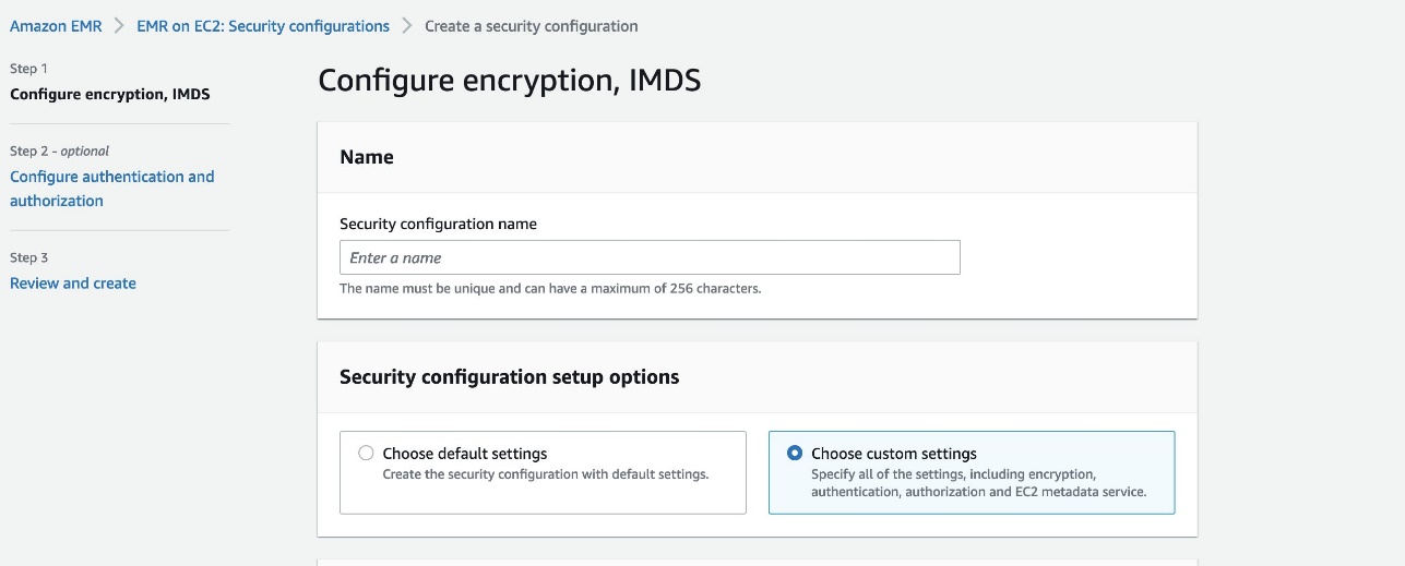
  1. On the Amazon EMR console, choose Security configurations in the navigation pane.
  2. Choose Create.
  3. Choose Create.
  4. For Security configuration name, enter a name.
  5. For Security configuration setup options, select Choose custom settings.
  6. For IAM role for applications, select Runtime role.
  7. Select Propagate source identity to audit actions performed using the runtime role.
  8. For Fine-grained access control, select AWS Lake Formation.
  9. Complete the security configuration.

The security configuration appears in your security configuration list. You can also see that the authorization mechanism listed here is the runtime role instead of the instance profile.

Launch the cluster

Now we launch an EMR cluster and specify the security configuration we created. For more information, refer to Specify a security configuration for a cluster.

The following code provides the AWS CLI command for launching an EMR cluster with the appropriate security configuration. Note that this cluster is launched on the default VPC and public subnet with the default IAM roles. In addition, the cluster is launched with one primary and one core instance of the specified instance type. For more details on how to customize the launch parameters, refer to create-cluster.

If the default EMR roles EMR_EC2_DefaultRole and EMR_DefaultRole don’t exist in IAM in your account (this is the first time you’re launching an EMR cluster with those), before launching the cluster, use the following command to create them:

aws emr create-default-roles

Create the cluster with the following code:

#Change with your Key Pair
KEYPAIR=<MY_KEYPAIR>
INSTANCE_TYPE="r4.4xlarge"
#Change with your Security Configuration Name
SECURITY_CONFIG="iamconfig-with-iam-lf"
#Change with your S3 log URI
LOG_URI="s3://mybucket/logs/"

aws emr create-cluster \
--name "iam-passthrough-cluster" \
--release-label emr-6.7.0 \
--use-default-roles \
--security-configuration $SECURITY_CONFIG \
--ec2-attributes KeyName=$KEYPAIR \
--instance-groups InstanceGroupType=MASTER,InstanceCount=1,InstanceType=$INSTANCE_TYPE  InstanceGroupType=CORE,InstanceCount=1,InstanceType=$INSTANCE_TYPE \
--applications Name=Spark Name=Hadoop Name=Hive \
--log-uri $LOG_URI

When the cluster is fully provisioned (Waiting state), let’s try to run a step on it with runtime roles for EMR steps enabled:

#Change with your EMR cluster ID
CLUSTER_ID=j-XXXXXXXXXXXXX
aws emr add-steps \
--cluster-id $CLUSTER_ID \
--steps '[{
            "Type": "CUSTOM_JAR",
            "ActionOnFailure": "CONTINUE",
            "Jar": "command-runner.jar",
            "Name": "Spark Example",
            "Args": [
              "spark-submit",
              "--class",
              "org.apache.spark.examples.SparkPi",
              "/usr/lib/spark/examples/jars/spark-examples.jar",
              "5"
            ]
        }]'

After launching the command, we receive the following as output:

An error occurred (ValidationException) when calling the AddJobFlowSteps operation: Runtime roles are required for this cluster. Please specify the role using the ExecutionRoleArn parameter.

The step failed, asking us to provide a runtime role. In the next section, we set up two IAM roles with different permissions and use them as the runtime roles for EMR steps.

Set up IAM roles as runtime roles

Any IAM role that you want to use as a runtime role for EMR steps must have a trust policy that allows the EMR cluster’s EC2 instance profile to assume it. In our setup, we’re using the default IAM role EMR_EC2_DefaultRole as the instance profile role. In addition, we create two IAM roles called test-emr-demo1 and test-emr-demo2 that we use as runtime roles for EMR steps.

The following code is the trust policy for both of the IAM roles, which lets the EMR cluster’s EC2 instance profile role, EMR_EC2_DefaultRole, assume these roles and set the source identity and LakeFormationAuthorizedCaller tag on the role sessions. The TagSession permission is needed so that Amazon EMR can authorize to Lake Formation. The SetSourceIdentity statement is needed for the propagate source identity feature.

Create a file called trust-policy.json with the following content (replace 123456789012 with your AWS account ID):

{
    "Version": "2012-10-17",
    "Statement": [
        {
            "Effect": "Allow",
            "Principal": {
                "AWS": "arn:aws:iam::123456789012:role/EMR_EC2_DefaultRole"
            },
            "Action": "sts:AssumeRole"
        },
        {
            "Effect": "Allow",
            "Principal": {
                "AWS": "arn:aws:iam::123456789012:role/EMR_EC2_DefaultRole"
            },
            "Action": "sts:SetSourceIdentity"
        },
        {
            "Effect": "Allow",
            "Principal": {
                "AWS": "arn:aws:iam::123456789012:role/EMR_EC2_DefaultRole"
            },
            "Action": "sts:TagSession",
            "Condition": {
                "StringEquals": {
                    "aws:RequestTag/LakeFormationAuthorizedCaller": "Amazon EMR"
                }
            }
        }
    ]
}

Use that policy to create the two IAM roles, test-emr-demo1 and test-emr-demo2:

aws iam create-role \
--role-name test-emr-demo1 \
--assume-role-policy-document file://trust-policy.json

aws iam create-role \
--role-name test-emr-demo2 \
--assume-role-policy-document file://trust-policy.json

Set up permissions for the principal submitting the EMR steps with runtime roles

The IAM principal submitting the EMR steps needs to have permissions to invoke the AddJobFlowSteps API. In addition, you can use the Condition key elasticmapreduce:ExecutionRoleArn to control access to specific IAM roles. For example, the following policy allows the IAM principal to only use IAM roles test-emr-demo1 and test-emr-demo2 as the runtime roles for EMR steps.

  1. Create the job-submitter-policy.json file with the following content (replace 123456789012 with your AWS account ID):
    {
        "Version": "2012-10-17",
        "Statement": [
            {
                "Sid": "AddStepsWithSpecificExecRoleArn",
                "Effect": "Allow",
                "Action": [
                    "elasticmapreduce:AddJobFlowSteps"
                ],
                "Resource": "*",
                "Condition": {
                    "StringEquals": {
                        "elasticmapreduce:ExecutionRoleArn": [
                            "arn:aws:iam::123456789012:role/test-emr-demo1",
                            "arn:aws:iam::123456789012:role/test-emr-demo2"
                        ]
                    }
                }
            },
            {
                "Sid": "EMRDescribeCluster",
                "Effect": "Allow",
                "Action": [
                    "elasticmapreduce:DescribeCluster"
                ],
                "Resource": "*"
            }
        ]
    }

  2. Create the IAM policy with the following code:
    aws iam create-policy \
    --policy-name emr-runtime-roles-submitter-policy \
    --policy-document file://job-submitter-policy.json

  3. Assign this policy to the IAM principal (IAM user or IAM role) you’re going to use to submit the EMR steps (replace 123456789012 with your AWS account ID and replace john with the IAM user you use to submit your EMR steps):
    aws iam attach-user-policy \
    --user-name john \
    --policy-arn "arn:aws:iam::123456789012:policy/emr-runtime-roles-submitter-policy"

IAM user john can now submit steps using arn:aws:iam::123456789012:role/test-emr-demo1 and arn:aws:iam::123456789012:role/test-emr-demo2 as the step runtime roles.

Use runtime roles with EMR steps

We now prepare our setup to show runtime roles for EMR steps in action.

Set up Amazon S3

To prepare your Amazon S3 data, complete the following steps:

  1. Create a CSV file called test.csv with the following content:
    1,a,1a
    2,b,2b

  2. Upload the file to Amazon S3 in three different locations:
    #Change this with your bucket name
    BUCKET_NAME="emr-steps-roles-new-us-east-1"
    
    aws s3 cp test.csv s3://${BUCKET_NAME}/demo1/
    aws s3 cp test.csv s3://${BUCKET_NAME}/demo2/
    aws s3 cp test.csv s3://${BUCKET_NAME}/nondemo/

    For our initial test, we use a PySpark application called test.py with the following contents:

    from pyspark.sql import SparkSession
    spark = SparkSession.builder.appName("my app").enableHiveSupport().getOrCreate()
    
    #Change this with your bucket name
    BUCKET_NAME="emr-steps-roles-new-us-east-1"
    
    try:
      spark.read.csv("s3://" + BUCKET_NAME + "/demo1/test.csv").show()
      print("Accessed demo1")
    except:
      print("Could not access demo1")
    
    try:
      spark.read.csv("s3://" + BUCKET_NAME + "/demo2/test.csv").show()
      print("Accessed demo2")
    except:
      print("Could not access demo2")
    
    try:
      spark.read.csv("s3://" + BUCKET_NAME + "/nondemo/test.csv").show()
      print("Accessed nondemo")
    except:
      print("Could not access nondemo")
    spark.stop()

    In the script, we’re trying to access the CSV file present under three different prefixes in the test bucket.

  3. Upload the Spark application inside the same S3 bucket where we placed the test.csv file but in a different location:
    #Change this with your bucket name
    BUCKET_NAME="emr-steps-roles-new-us-east-1"
    aws s3 cp test.py s3://${BUCKET_NAME}/scripts/

Set up runtime role permissions

To show how runtime roles for EMR steps works, we assign to the roles we created different IAM permissions to access Amazon S3. The following table summarizes the grants we provide to each role (emr-steps-roles-new-us-east-1 is the bucket you configured in the previous section).

S3 locations \ IAM Roles test-emr-demo1 test-emr-demo2
s3://emr-steps-roles-new-us-east-1/* No Access No Access
s3://emr-steps-roles-new-us-east-1/demo1/* Full Access No Access
s3://emr-steps-roles-new-us-east-1/demo2/* No Access Full Access
s3://emr-steps-roles-new-us-east-1/scripts/* Read Access Read Access
  1. Create the file demo1-policy.json with the following content (substitute emr-steps-roles-new-us-east-1 with your bucket name):
    {
        "Version": "2012-10-17",
        "Statement": [
            {
                "Effect": "Allow",
                "Action": [
                    "s3:*"
                ],
                "Resource": [
                    "arn:aws:s3:::emr-steps-roles-new-us-east-1/demo1",
                    "arn:aws:s3:::emr-steps-roles-new-us-east-1/demo1/*"
                ]                    
            },
            {
                "Effect": "Allow",
                "Action": [
                    "s3:Get*"
                ],
                "Resource": [
                    "arn:aws:s3:::emr-steps-roles-new-us-east-1/scripts",
                    "arn:aws:s3:::emr-steps-roles-new-us-east-1/scripts/*"
                ]                    
            }
        ]
    }

  2. Create the file demo2-policy.json with the following content (substitute emr-steps-roles-new-us-east-1 with your bucket name):
    {
        "Version": "2012-10-17",
        "Statement": [
            {
                "Effect": "Allow",
                "Action": [
                    "s3:*"
                ],
                "Resource": [
                    "arn:aws:s3:::emr-steps-roles-new-us-east-1/demo2",
                    "arn:aws:s3:::emr-steps-roles-new-us-east-1/demo2/*"
                ]                    
            },
            {
                "Effect": "Allow",
                "Action": [
                    "s3:Get*"
                ],
                "Resource": [
                    "arn:aws:s3:::emr-steps-roles-new-us-east-1/scripts",
                    "arn:aws:s3:::emr-steps-roles-new-us-east-1/scripts/*"
                ]                    
            }
        ]
    }

  3. Create our IAM policies:
    aws iam create-policy \
    --policy-name test-emr-demo1-policy \
    --policy-document file://demo1-policy.json
    
    aws iam create-policy \
    --policy-name test-emr-demo2-policy \
    --policy-document file://demo2-policy.json

  4. Assign to each role the related policy (replace 123456789012 with your AWS account ID):
    aws iam attach-role-policy \
    --role-name test-emr-demo1 \
    --policy-arn "arn:aws:iam::123456789012:policy/test-emr-demo1-policy"
    
    aws iam attach-role-policy \
    --role-name test-emr-demo2 \
    --policy-arn "arn:aws:iam::123456789012:policy/test-emr-demo2-policy"

    To use runtime roles with Amazon EMR steps, we need to add the following policy to our EMR cluster’s EC2 instance profile (in this example EMR_EC2_DefaultRole). With this policy, the underlying EC2 instances for the EMR cluster can assume the runtime role and apply a tag to that runtime role.

  5. Create the file runtime-roles-policy.json with the following content (replace 123456789012 with your AWS account ID):
    {
        "Version": "2012-10-17",
        "Statement": [{
                "Sid": "AllowRuntimeRoleUsage",
                "Effect": "Allow",
                "Action": [
                    "sts:AssumeRole",
                    "sts:TagSession",
                    "sts:SetSourceIdentity"
                ],
                "Resource": [
                    "arn:aws:iam::123456789012:role/test-emr-demo1",
                    "arn:aws:iam::123456789012:role/test-emr-demo2"
                ]
            }
        ]
    }

  6. Create the IAM policy:
    aws iam create-policy \
    --policy-name emr-runtime-roles-policy \
    --policy-document file://runtime-roles-policy.json

  7. Assign the created policy to the EMR cluster’s EC2 instance profile, in this example EMR_EC2_DefaultRole:
    aws iam attach-role-policy \
    --role-name EMR_EC2_DefaultRole \
    --policy-arn "arn:aws:iam::123456789012:policy/emr-runtime-roles-policy"

Test permissions with runtime roles

We’re now ready to perform our first test. We run the test.py script, previously uploaded to Amazon S3, two times as Spark steps: first using the test-emr-demo1 role and then using the test-emr-demo2 role as the runtime roles.

To run an EMR step specifying a runtime role, you need the latest version of the AWS CLI. For more details about updating the AWS CLI, refer to Installing or updating the latest version of the AWS CLI.

Let’s submit a step specifying test-emr-demo1 as the runtime role:

#Change with your EMR cluster ID
CLUSTER_ID=j-XXXXXXXXXXXXX
#Change with your AWS Account ID
ACCOUNT_ID=123456789012
#Change with your Bucket name
BUCKET_NAME=emr-steps-roles-new-us-east-1

aws emr add-steps \
--cluster-id $CLUSTER_ID \
--steps '[{
            "Type": "CUSTOM_JAR",
            "ActionOnFailure": "CONTINUE",
            "Jar": "command-runner.jar",
            "Name": "Spark Example",
            "Args": [
              "spark-submit",
              "s3://'"${BUCKET_NAME}"'/scripts/test.py"
            ]
        }]' \
--execution-role-arn arn:aws:iam::${ACCOUNT_ID}:role/test-emr-demo1

This command returns an EMR step ID. To check our step output logs, we can proceed two different ways:

  • From the Amazon EMR console – On the Steps tab, choose the View logs link related to the specific step ID and select stdout.
  • From Amazon S3 – While launching our cluster, we configured an S3 location for logging. We can find our step logs under $(LOG_URI)/steps/<stepID>/stdout.gz.

The logs could take a couple of minutes to populate after the step is marked as Completed.

The following is the output of the EMR step with test-emr-demo1 as the runtime role:

+---+---+---+
|_c0|_c1|_c2|
+---+---+---+
|  1|  a| 1a|
|  2|  b| 2b|
+---+---+---+

Accessed demo1
Could not access demo2
Could not access nondemo

As we can see, only the demo1 folder was accessible by our application.

Diving deeper into the step stderr logs, we can see that the related YARN application application_1656350436159_0017 was launched with the user 6GC64F33KUW4Q2JY6LKR7UAHWETKKXYL. We can confirm this by connecting to the EMR primary instance using SSH and using the YARN CLI:

[hadoop@ip-172-31-63-203]$ yarn application -status application_1656350436159_0017
...
Application-Id : application_1656350436159_0017
Application-Name : my app
Application-Type : SPARK
User : 6GC64F33KUW4Q2JY6LKR7UAHWETKKXYL
Queue : default
Application Priority : 0
...

Please note that in your case, the YARN application ID and the user will be different.

Now we submit the same script again as a new EMR step, but this time with the role test-emr-demo2 as the runtime role:

#Change with your EMR cluster ID
CLUSTER_ID=j-XXXXXXXXXXXXX
#Change with your AWS Account ID
ACCOUNT_ID=123456789012
#Change with your Bucket name
BUCKET_NAME=emr-steps-roles-new-us-east-1

aws emr add-steps \
--cluster-id $CLUSTER_ID \
--steps '[{
            "Type": "CUSTOM_JAR",
            "ActionOnFailure": "CONTINUE",
            "Jar": "command-runner.jar",
            "Name": "Spark Example",
            "Args": [
              "spark-submit",
              "s3://'"${BUCKET_NAME}"'/scripts/test.py"
            ]
        }]' \
--execution-role-arn arn:aws:iam::${ACCOUNT_ID}:role/test-emr-demo2

The following is the output of the EMR step with test-emr-demo2 as the runtime role:

Could not access demo1
+---+---+---+
|_c0|_c1|_c2|
+---+---+---+
|  1|  a| 1a|
|  2|  b| 2b|
+---+---+---+

Accessed demo2
Could not access nondemo

As we can see, only the demo2 folder was accessible by our application.

Diving deeper into the step stderr logs, we can see that the related YARN application application_1656350436159_0018 was launched with a different user 7T2ORHE6Z4Q7PHLN725C2CVWILZWYOLE. We can confirm this by using the YARN CLI:

[hadoop@ip-172-31-63-203]$ yarn application -status application_1656350436159_0018
...
Application-Id : application_1656350436159_0018
Application-Name : my app
Application-Type : SPARK
User : 7T2ORHE6Z4Q7PHLN725C2CVWILZWYOLE
Queue : default
Application Priority : 0
...

Each step was able to only access the CSV file that was allowed by the runtime role, so the first step was able to only access s3://emr-steps-roles-new-us-east-1/demo1/test.csv and the second step was only able to access s3://emr-steps-roles-new-us-east-1/demo2/test.csv. In addition, we observed that Amazon EMR created a unique user for the steps, and used the user to run the jobs. Please note that both roles need at least read access to the S3 location where the step scripts are located (for example, s3://emr-steps-roles-demo-bucket/scripts/test.py).

Now that we have seen how runtime roles for EMR steps work, let’s look at how we can use Lake Formation to apply fine-grained access controls with EMR steps.

Use Lake Formation-based access control with EMR steps

You can use Lake Formation to apply table- and column-level permissions with Apache Spark and Apache Hive jobs submitted as EMR steps. First, the data lake admin in Lake Formation needs to register Amazon EMR as the AuthorizedSessionTagValue to enforce Lake Formation permissions on EMR. Lake Formation uses this session tag to authorize callers and provide access to the data lake. The Amazon EMR value is referenced inside the step-runtime-roles-sec-cfg.json file we used earlier when we created the EMR security configuration, and inside the trust-policy.json file we used to create the two runtime roles test-emr-demo1 and test-emr-demo2.

We can do so on the Lake Formation console in the External data filtering section (replace 123456789012 with your AWS account ID).

On the IAM runtime roles’ trust policy, we already have the sts:TagSession permission with the condition “aws:RequestTag/LakeFormationAuthorizedCaller": "Amazon EMR". So we’re ready to proceed.

To demonstrate how Lake Formation works with EMR steps, we create one database named entities with two tables named users and products, and we assign in Lake Formation the grants summarized in the following table.

IAM Roles \ Tables entities
(DB)
users
(Table)
products
(Table)
test-emr-demo1 Full Read Access No Access
test-emr-demo2 Read Access on Columns: uid, state Full Read Access

Prepare Amazon S3 files

We first prepare our Amazon S3 files.

  1. Create the users.csv file with the following content:
    00005678,john,pike,england,london,Hidden Road 78
    00009039,paolo,rossi,italy,milan,Via degli Alberi 56A
    00009057,july,finn,germany,berlin,Green Road 90

  2. Create the products.csv file with the following content:
    P0000789,Bike2000,Sport
    P0000567,CoverToCover,Smartphone
    P0005677,Whiteboard X786,Home

  3. Upload these files to Amazon S3 in two different locations:
    #Change this with your bucket name
    BUCKET_NAME="emr-steps-roles-new-us-east-1"
    
    aws s3 cp users.csv s3://${BUCKET_NAME}/entities-database/users/
    aws s3 cp products.csv s3://${BUCKET_NAME}/entities-database/products/

Prepare the database and tables

We can create our entities database by using the AWS Glue APIs.

  1. Create the entities-db.json file with the following content (substitute emr-steps-roles-new-us-east-1 with your bucket name):
    {
        "DatabaseInput": {
            "Name": "entities",
            "LocationUri": "s3://emr-steps-roles-new-us-east-1/entities-database/",
            "CreateTableDefaultPermissions": []
        }
    }

  2. With a Lake Formation admin user, run the following command to create our database:
    aws glue create-database \
    --cli-input-json file://entities-db.json

    We also use the AWS Glue APIs to create the tables users and products.

  3. Create the users-table.json file with the following content (substitute emr-steps-roles-new-us-east-1 with your bucket name):
    {
        "TableInput": {
            "Name": "users",
            "StorageDescriptor": {
                "Columns": [{
                        "Name": "uid",
                        "Type": "string"
                    },
                    {
                        "Name": "name",
                        "Type": "string"
                    },
                    {
                        "Name": "surname",
                        "Type": "string"
                    },
                    {
                        "Name": "state",
                        "Type": "string"
                    },
                    {
                        "Name": "city",
                        "Type": "string"
                    },
                    {
                        "Name": "address",
                        "Type": "string"
                    }
                ],
                "Location": "s3://emr-steps-roles-new-us-east-1/entities-database/users/",
                "InputFormat": "org.apache.hadoop.mapred.TextInputFormat",
                "OutputFormat": "org.apache.hadoop.hive.ql.io.HiveIgnoreKeyTextOutputFormat",
                "Compressed": false,
                "SerdeInfo": {
                    "SerializationLibrary": "org.apache.hadoop.hive.serde2.lazy.LazySimpleSerDe",
                    "Parameters": {
                        "field.delim": ",",
                        "serialization.format": ","
                    }
                }
            },
            "TableType": "EXTERNAL_TABLE",
            "Parameters": {
                "EXTERNAL": "TRUE"
            }
        }
    }

  4. Create the products-table.json file with the following content (substitute emr-steps-roles-new-us-east-1 with your bucket name):
    {
        "TableInput": {
            "Name": "products",
            "StorageDescriptor": {
                "Columns": [{
                        "Name": "product_id",
                        "Type": "string"
                    },
                    {
                        "Name": "name",
                        "Type": "string"
                    },
                    {
                        "Name": "category",
                        "Type": "string"
                    }
                ],
                "Location": "s3://emr-steps-roles-new-us-east-1/entities-database/products/",
                "InputFormat": "org.apache.hadoop.mapred.TextInputFormat",
                "OutputFormat": "org.apache.hadoop.hive.ql.io.HiveIgnoreKeyTextOutputFormat",
                "Compressed": false,
                "SerdeInfo": {
                    "SerializationLibrary": "org.apache.hadoop.hive.serde2.lazy.LazySimpleSerDe",
                    "Parameters": {
                        "field.delim": ",",
                        "serialization.format": ","
                    }
                }
            },
            "TableType": "EXTERNAL_TABLE",
            "Parameters": {
                "EXTERNAL": "TRUE"
            }
        }
    }

  5. With a Lake Formation admin user, create our tables with the following commands:
    aws glue create-table \
        --database-name entities \
        --cli-input-json file://users-table.json
        
    aws glue create-table \
        --database-name entities \
        --cli-input-json file://products-table.json

Set up the Lake Formation data lake locations

To access our tables data in Amazon S3, Lake Formation needs read/write access to them. To achieve that, we have to register Amazon S3 locations where our data resides and specify for them which IAM role to obtain credentials from.

Let’s create our IAM role for the data access.

  1. Create a file called trust-policy-data-access-role.json with the following content:
    {
        "Version": "2012-10-17",
        "Statement": [
            {
                "Sid": "",
                "Effect": "Allow",
                "Principal": {
                    "Service": "lakeformation.amazonaws.com"
                },
                "Action": "sts:AssumeRole"
            }
        ]
    }

  2. Use the policy to create the IAM role emr-demo-lf-data-access-role:
    aws iam create-role \
    --role-name emr-demo-lf-data-access-role \
    --assume-role-policy-document file://trust-policy-data-access-role.json

  3. Create the file data-access-role-policy.json with the following content (substitute emr-steps-roles-new-us-east-1 with your bucket name):
    {
        "Version": "2012-10-17",
        "Statement": [
            {
                "Effect": "Allow",
                "Action": [
                    "s3:*"
                ],
                "Resource": [
                    "arn:aws:s3:::emr-steps-roles-new-us-east-1/entities-database",
                    "arn:aws:s3:::emr-steps-roles-new-us-east-1/entities-database/*"
                ]
            },
            {
                "Effect": "Allow",
                "Action": [
                    "s3:ListBucket"
                ],
                "Resource": [
                    "arn:aws:s3:::emr-steps-roles-new-us-east-1"
                ]
            }
        ]
    }

  4. Create our IAM policy:
    aws iam create-policy \
    --policy-name data-access-role-policy \
    --policy-document file://data-access-role-policy.json

  5. Assign to our emr-demo-lf-data-access-role the created policy (replace 123456789012 with your AWS account ID):
    aws iam attach-role-policy \
    --role-name emr-demo-lf-data-access-role \
    --policy-arn "arn:aws:iam::123456789012:policy/data-access-role-policy"

    We can now register our data location in Lake Formation.

  6. On the Lake Formation console, choose Data lake locations in the navigation pane.
  7. Here we can register our S3 location containing data for our two tables and choose the created emr-demo-lf-data-access-role IAM role, which has read/write access to that location.

For more details about adding an Amazon S3 location to your data lake and configuring your IAM data access roles, refer to Adding an Amazon S3 location to your data lake.

Enforce Lake Formation permissions

To be sure we’re using Lake Formation permissions, we should confirm that we don’t have any grants set up for the principal IAMAllowedPrincipals. The IAMAllowedPrincipals group includes any IAM users and roles that are allowed access to your Data Catalog resources by your IAM policies, and it’s used to maintain backward compatibility with AWS Glue.

To confirm Lake Formations permissions are enforced, navigate to the Lake Formation console and choose Data lake permissions in the navigation pane. Filter permissions by “Database”:“entities” and remove all the permissions given to the principal IAMAllowedPrincipals.

For more details on IAMAllowedPrincipals and backward compatibility with AWS Glue, refer to Changing the default security settings for your data lake.

Configure AWS Glue and Lake Formation grants for IAM runtime roles

To allow our IAM runtime roles to properly interact with Lake Formation, we should provide them the lakeformation:GetDataAccess and glue:Get* grants.

Lake Formation permissions control access to Data Catalog resources, Amazon S3 locations, and the underlying data at those locations. IAM permissions control access to the Lake Formation and AWS Glue APIs and resources. Therefore, although you might have the Lake Formation permission to access a table in the Data Catalog (SELECT), your operation fails if you don’t have the IAM permission on the glue:Get* API.

For more details about Lake Formation access control, refer to Lake Formation access control overview.

  1. Create the emr-runtime-roles-lake-formation-policy.json file with the following content:
    {
        "Version": "2012-10-17",
        "Statement": {
            "Sid": "LakeFormationManagedAccess",
            "Effect": "Allow",
            "Action": [
                "lakeformation:GetDataAccess",
                "glue:Get*",
                "glue:Create*",
                "glue:Update*"
            ],
            "Resource": "*"
        }
    }

  2. Create the related IAM policy:
    aws iam create-policy \
    --policy-name emr-runtime-roles-lake-formation-policy \
    --policy-document file://emr-runtime-roles-lake-formation-policy.json

  3. Assign this policy to both IAM runtime roles (replace 123456789012 with your AWS account ID):
    aws iam attach-role-policy \
    --role-name test-emr-demo1 \
    --policy-arn "arn:aws:iam::123456789012:policy/emr-runtime-roles-lake-formation-policy"
    
    aws iam attach-role-policy \
    --role-name test-emr-demo2 \
    --policy-arn "arn:aws:iam::123456789012:policy/emr-runtime-roles-lake-formation-policy"

Set up Lake Formation permissions

We now set up the permission in Lake Formation for the two runtime roles.

  1. Create the file users-grants-test-emr-demo1.json with the following content to grant SELECT access to all columns in the entities.users table to test-emr-demo1:
    {
        "Principal": {
            "DataLakePrincipalIdentifier": "arn:aws:iam::123456789012:role/test-emr-demo1"
        },
        "Resource": {
            "Table": {
                "DatabaseName": "entities",
                "Name": "users"
            }
        },
        "Permissions": [
            "SELECT"
        ]
    }

  2. Create the file users-grants-test-emr-demo2.json with the following content to grant SELECT access to the uid and state columns in the entities.users table to test-emr-demo2:
    {
        "Principal": {
            "DataLakePrincipalIdentifier": "arn:aws:iam::123456789012:role/test-emr-demo2"
        },
        "Resource": {
            "TableWithColumns": {
                "DatabaseName": "entities",
                "Name": "users",
                "ColumnNames": ["uid", "state"]
            }
        },
        "Permissions": [
            "SELECT"
        ]
    }

  3. Create the file products-grants-test-emr-demo2.json with the following content to grant SELECT access to all columns in the entities.products table to test-emr-demo2:
    {
        "Principal": {
            "DataLakePrincipalIdentifier": "arn:aws:iam::123456789012:role/test-emr-demo2"
        },
        "Resource": {
            "Table": {
                "DatabaseName": "entities",
                "Name": "products"
            }
        },
        "Permissions": [
            "SELECT"
        ]
    }

  4. Let’s set up our permissions in Lake Formation:
    aws lakeformation grant-permissions \
    --cli-input-json file://users-grants-test-emr-demo1.json
    
    aws lakeformation grant-permissions \
    --cli-input-json file://users-grants-test-emr-demo2.json
    
    aws lakeformation grant-permissions \
    --cli-input-json file://products-grants-test-emr-demo2.json

  5. Check the permissions we defined on the Lake Formation console on the Data lake permissions page by filtering by “Database”:“entities”.

Test Lake Formation permissions with runtime roles

For our test, we use a PySpark application called test-lake-formation.py with the following content:


from pyspark.sql import SparkSession
 
spark = SparkSession.builder.appName("Pyspark - TEST IAM RBAC with LF").enableHiveSupport().getOrCreate()

try:
    print("== select * from entities.users limit 3 ==\n")
    spark.sql("select * from entities.users limit 3").show()
except Exception as e:
    print(e)

try:
    print("== select * from entities.products limit 3 ==\n")
    spark.sql("select * from entities.products limit 3").show()
except Exception as e:
    print(e)

spark.stop()

In the script, we’re trying to access the tables users and products. Let’s upload our Spark application in the same S3 bucket that we used earlier:

#Change this with your bucket name
BUCKET_NAME="emr-steps-roles-new-us-east-1"

aws s3 cp test-lake-formation.py s3://${BUCKET_NAME}/scripts/

We’re now ready to perform our test. We run the test-lake-formation.py script first using the test-emr-demo1 role and then using the test-emr-demo2 role as the runtime roles.

Let’s submit a step specifying test-emr-demo1 as the runtime role:

#Change with your EMR cluster ID
CLUSTER_ID=j-XXXXXXXXXXXXX
#Change with your AWS Account ID
ACCOUNT_ID=123456789012
#Change with your Bucket name
BUCKET_NAME=emr-steps-roles-new-us-east-1

aws emr add-steps \
--cluster-id $CLUSTER_ID \
--steps '[{
            "Type": "CUSTOM_JAR",
            "ActionOnFailure": "CONTINUE",
            "Jar": "command-runner.jar",
            "Name": "Spark Lake Formation Example",
            "Args": [
              "spark-submit",
              "s3://'"${BUCKET_NAME}"'/scripts/test-lake-formation.py"
            ]
        }]' \
--execution-role-arn arn:aws:iam::${ACCOUNT_ID}:role/test-emr-demo1

The following is the output of the EMR step with test-emr-demo1 as the runtime role:

== select * from entities.users limit 3 ==

+--------+-----+-------+-------+------+--------------------+
|     uid| name|surname|  state|  city|             address|
+--------+-----+-------+-------+------+--------------------+
|00005678| john|   pike|england|london|      Hidden Road 78|
|00009039|paolo|  rossi|  italy| milan|Via degli Alberi 56A|
|00009057| july|   finn|germany|berlin|       Green Road 90|
+--------+-----+-------+-------+------+--------------------+

== select * from entities.products limit 3 ==

Insufficient Lake Formation permission(s) on products (...)

As we can see, our application was only able to access the users table.

Submit the same script again as a new EMR step, but this time with the role test-emr-demo2 as the runtime role:

#Change with your EMR cluster ID
CLUSTER_ID=j-XXXXXXXXXXXXX
#Change with your AWS Account ID
ACCOUNT_ID=123456789012
#Change with your Bucket name
BUCKET_NAME=emr-steps-roles-new-us-east-1

aws emr add-steps \
--cluster-id $CLUSTER_ID \
--steps '[{
            "Type": "CUSTOM_JAR",
            "ActionOnFailure": "CONTINUE",
            "Jar": "command-runner.jar",
            "Name": "Spark Lake Formation Example",
            "Args": [
              "spark-submit",
              "s3://'"${BUCKET_NAME}"'/scripts/test-lake-formation.py"
            ]
        }]' \
--execution-role-arn arn:aws:iam::${ACCOUNT_ID}:role/test-emr-demo2

The following is the output of the EMR step with test-emr-demo2 as the runtime role:

== select * from entities.users limit 3 ==

+--------+-------+
|     uid|  state|
+--------+-------+
|00005678|england|
|00009039|  italy|
|00009057|germany|
+--------+-------+

== select * from entities.products limit 3 ==

+----------+---------------+----------+
|product_id|           name|  category|
+----------+---------------+----------+
|  P0000789|       Bike2000|     Sport|
|  P0000567|   CoverToCover|Smartphone|
|  P0005677|Whiteboard X786|      Home|
+----------+---------------+----------+

As we can see, our application was able to access a subset of columns for the users table and all the columns for the products table.

We can conclude that the permissions while accessing the Data Catalog are being enforced based on the runtime role used with the EMR step.

Audit using the source identity

The source identity is a mechanism to monitor and control actions taken with assumed roles. The Propagate source identity feature similarly allows you to monitor and control actions taken using runtime roles by the jobs submitted with EMR steps.

We already configured EMR_EC2_defaultRole with "sts:SetSourceIdentity" on our two runtime roles. Also, both runtime roles let EMR_EC2_DefaultRole to SetSourceIdentity in their trust policy. So we’re ready to proceed.

We now see the Propagate source identity feature in action with a simple example.

Configure the IAM role that is assumed to submit the EMR steps

We configure the IAM role job-submitter-1, which is assumed specifying the source identity and which is used to submit the EMR steps. In this example, we allow the IAM user paul to assume this role and set the source identity. Please note you can use any IAM principal here.

  1. Create a file called trust-policy-2.json with the following content (replace 123456789012 with your AWS account ID):
    {
        "Version": "2012-10-17",
        "Statement": [
            {
                "Effect": "Allow",
                "Principal": {
                    "AWS": "arn:aws:iam::123456789012:user/paul"
                },
                "Action": "sts:AssumeRole"
            },
            {
                "Effect": "Allow",
                "Principal": {
                    "AWS": "arn:aws:iam::123456789012:user/paul"
                },
                "Action": "sts:SetSourceIdentity"
            }
        ]
    }

  2. Use it as the trust policy to create the IAM role job-submitter-1:
    aws iam create-role \
    --role-name job-submitter-1 \
    --assume-role-policy-document file://trust-policy-2.json

    We use now the same emr-runtime-roles-submitter-policy policy we defined before to allow the role to submit EMR steps using the test-emr-demo1 and test-emr-demo2 runtime roles.

  3. Assign this policy to the IAM role job-submitter-1 (replace 123456789012 with your AWS account ID):
    aws iam attach-role-policy \
    --role-name job-submitter-1 \
    --policy-arn "arn:aws:iam::123456789012:policy/emr-runtime-roles-submitter-policy"

Test the source identity with AWS CloudTrail

To show how propagation of source identity works with Amazon EMR, we generate a role session with the source identity test-ad-user.

With the IAM user paul (or with the IAM principal you configured), we first perform the impersonation (replace 123456789012 with your AWS account ID):

aws sts assume-role \
--role-arn arn:aws:iam::123456789012:role/job-submitter-1 \
--role-session-name demotest \
--source-identity test-ad-user

The following code is the output received:

{
"Credentials": {
    "SecretAccessKey": "<SECRET_ACCESS_KEY>",
    "SessionToken": "<SESSION_TOKEN>",
    "Expiration": "<EXPIRATION_TIME>",
    "AccessKeyId": "<ACCESS_KEY_ID>"
},
"AssumedRoleUser": {
    "AssumedRoleId": "AROAUVT2HQ3......:demotest",
    "Arn": "arn:aws:sts::123456789012:assumed-role/test-emr-role/demotest"
},
"SourceIdentity": "test-ad-user"
}

We use the temporary AWS security credentials of the role session, to submit an EMR step along with the runtime role test-emr-demo1:

export AWS_ACCESS_KEY_ID="<ACCESS_KEY_ID>"
export AWS_SECRET_ACCESS_KEY="<SECRET_ACCESS_KEY>"
export AWS_SESSION_TOKEN="<SESSION_TOKEN>" 

#Change with your EMR cluster ID
CLUSTER_ID=j-XXXXXXXXXXXXX
#Change with your AWS Account ID
ACCOUNT_ID=123456789012
#Change with your Bucket name
BUCKET_NAME=emr-steps-roles-new-us-east-1

aws emr add-steps \
--cluster-id $CLUSTER_ID \
--steps '[{
            "Type": "CUSTOM_JAR",
            "ActionOnFailure": "CONTINUE",
            "Jar": "command-runner.jar",
            "Name": "Spark Lake Formation Example",
            "Args": [
              "spark-submit",
              "s3://'"${BUCKET_NAME}"'/scripts/test-lake-formation.py"
            ]
        }]' \
--execution-role-arn arn:aws:iam::${ACCOUNT_ID}:role/test-emr-demo1

In a few minutes, we can see events appearing in the AWS CloudTrail log file. We can see all the AWS APIs that the jobs invoked using the runtime role. In the following snippet, we can see that the step performed the sts:AssumeRole and lakeformation:GetDataAccess actions. It’s worth noting how the source identity test-ad-user has been preserved in the events.

Clean up

You can now delete the EMR cluster you created.

  1. On the Amazon EMR console, choose Clusters in the navigation pane.
  2. Select the cluster iam-passthrough-cluster, then choose Terminate.
  3. Choose Terminate again to confirm.

Alternatively, you can delete the cluster by using the Amazon EMR CLI with the following command (replace the EMR cluster ID with the one returned by the previously run aws emr create-cluster command):

aws emr terminate-clusters --cluster-ids j-3KVXXXXXXX7UG

Conclusion

In this post, we discussed how you can control data access on Amazon EMR on EC2 clusters by using runtime roles with EMR steps. We discussed how the feature works, how you can use Lake Formation to apply fine-grained access controls, and how to monitor and control actions using a source identity. To learn more about this feature, refer to Configure runtime roles for Amazon EMR steps.


About the authors

Stefano Sandona is an Analytics Specialist Solution Architect with AWS. He loves data, distributed systems and security. He helps customers around the world architecting their data platforms. He has a strong focus on Amazon EMR and all the security aspects around it.

Sharad Kala is a senior engineer at AWS working with the EMR team. He focuses on the security aspects of the applications running on EMR. He has a keen interest in working and learning about distributed systems.

Get started with Apache Hudi using AWS Glue by implementing key design concepts – Part 1

Post Syndicated from Amit Maindola original https://aws.amazon.com/blogs/big-data/part-1-get-started-with-apache-hudi-using-aws-glue-by-implementing-key-design-concepts/

Many organizations build data lakes on Amazon Simple Storage Service (Amazon S3) using a modern architecture for a scalable and cost-effective solution. Open-source storage formats like Parquet and Avro are commonly used, and data is stored in these formats as immutable files. As the data lake is expanded to additional use cases, there are still some use cases that are very difficult with data lakes, such as CDC (change data capture), time travel (querying point-in-time data), privacy regulation requiring deletion of data, concurrent writes, and consistency regarding handling small file problems.

Apache Hudi is an open-source transactional data lake framework that greatly simplifies incremental data processing and streaming data ingestion. However, organizations new to data lakes may struggle to adopt Apache Hudi due to unfamiliarity with the technology and lack of internal expertise.

In this post, we show how to get started with Apache Hudi, focusing on the Hudi CoW (Copy on Write) table type on AWS using AWS Glue, and implementing key design concepts for different use cases. We expect readers to have a basic understanding of data lakes, AWS Glue, and Amazon S3. We walk you through common batch data ingestion use cases with actual test results using a TPC-DS dataset to show how the design decisions can influence the outcome.

Apache Hudi key concepts

Before diving deep into the design concepts, let’s review the key concepts of Apache Hudi, which is important to understand before you make design decisions.

Hudi table and query types

Hudi supports two table types: Copy on Write (CoW) and Merge on Read (MoR). You have to choose the table type in advance, which influences the performance of read and write operations.

The difference in performance depends on the volume of data, operations, file size, and other factors. For more information, refer to Table & Query Types.

When you use the CoW table type, committed data is implicitly compacted, meaning it’s updated to columnar file format during write operation. With the MoR table type, data isn’t compacted with every commit. As a result, for the MoR table type, compacted data lives in columnar storage (Parquet) and deltas are stored in a log (Avro) raw format until compaction merges changes the data to columnar file format. Hudi supports snapshot, incremental, and read-optimized queries for Hudi tables, and the output of the result depends on the query type.

Indexing

Indexing is another key concept for the design. Hudi provides efficient upserts and deletes with fast indexing for both CoW and MoR tables. For CoW tables, indexing enables fast upsert and delete operations by avoiding the need to join against the entire dataset to determine which files to rewrite. For MoR, this design allows Hudi to bound the amount of records any given base file needs to be merged against. Specifically, a given base file needs to be merged only against updates for records that are part of that base file. In contrast, designs without an indexing component could end up having to merge all the base files against all incoming update and delete records.

Solution overview

The following diagram describes the high-level architecture for our solution. We ingest the TPC-DS (store_sales) dataset from the source S3 bucket in CSV format and write it to the target S3 bucket using AWS Glue in Hudi format. We can query the Hudi tables on Amazon S3 using Amazon Athena and AWS Glue Studio Notebooks.

The following diagram illustrates the relationships between our tables.

For our post, we use the following tables from the TPC-DS dataset: one fact table, store_sales, and the dimension tables store, item, and date_dim. The following table summarizes the table row counts.

Table Approximate Row Counts
store_sales 2.8 billion
store 1,000
item 300,000
date_dim 73,000

Set up the environment

After you sign in to your test AWS account, launch the provided AWS CloudFormation template by choosing Launch Stack:

Launch Button

This template configures the following resources:

  • AWS Glue jobs hudi_bulk_insert, hudi_upsert_cow, and hudi_bulk_insert_dim. We use these jobs for the use cases covered in this post.
  • An S3 bucket to store the output of the AWS Glue job runs.
  • AWS Identity and Access Management (IAM) roles and policies with appropriate permissions.

Before you run the AWS Glue jobs, you need to subscribe to the AWS Glue Apache Hudi Connector (latest version: 0.10.1). The connector is available on AWS Marketplace. Follow the connector installation and activation process from the AWS Marketplace link, or refer to Process Apache Hudi, Delta Lake, Apache Iceberg datasets at scale, part 1: AWS Glue Studio Notebook to set it up.

After you create the Hudi connection, add the connector name to all the AWS Glue scripts under Advanced properties.

Bulk insert job

To run the bulk insert job, choose the job hudi_bulk_insert on the AWS Glue console.

The job parameters as shown in the following screenshot are added as part of the CloudFormation stack setup. You can use different values to create CoW partitioned tables with different bulk insert options.

The parameters are as follows:

  • HUDI_DB_NAME – The database in the AWS Glue Data Catalog where the catalog table is created.
  • HUDI_INIT_SORT_OPTION – The options for bulk_insert include GLOBAL_SORT, which is the default. Other options include NONE and PARTITION_SORT.
  • HUDI_TABLE_NAME – The table name prefix that you want to use to identify the table created. In the code, we append the sort option to the name you specify in this parameter.
  • OUTPUT_BUCKET – The S3 bucket created through the CloudFormation stack where the Hudi table datasets are written. The bucket name format is <account number><bucket name>. The bucket name is the one given while creating the CloudFormation stack.
  • CATEGORY_ID – The default for this parameter is ALL, which processes categories of test data in a single AWS Glue job. To test the parallel on the same table, change the parameter value to one of categories from 3, 5, or 8 for the dataset that we use for each parallel AWS Glue job.

Upsert job for the CoW table

To run the upsert job, choose the job hudi_upsert_cow on the AWS Glue console.

The following job parameters are added as part of the CloudFormation stack setup. You can run upsert and delete operations on CoW partitioned tables with different bulk insert options based on the values provided for these parameters.

  • OUTPUT-BUCKET – The same value as the previous job parameter.
  • HUDI_TABLE_NAME – The name of the table created in your AWS Glue Data Catalog.
  • HUDI_DB_NAME – The same value as the previous job parameter. The default value is Default.

Bulk insert job for the Dimension tables

To test the queries on the CoW tables, the fact table that is created using the bulk insert operation needs supplemental dimensional tables. This AWS Glue job has to be run before you can test the TPC queries provided later in this post. To run this job, choose hudi_bulk_insert_dim on the AWS Glue console and use the parameters shown in the following screenshot.

The parameters are as follows:

  • OUTPUT-BUCKET – The same value as the previous job parameter.
  • HUDI_INIT_SORT_OPTION – The options for bulk_insert include GLOBAL_SORT, which is the default. Other available options are NONE and PARTITION_SORT.
  • HUDI_DB_NAME – The Hudi database name. Default is the default value.

Hudi design considerations

In this section, we walk you through a few use cases to demonstrate the difference in the outcome for different settings and operations.

Data migration use case

In Apache Hudi, you ingest the data into CoW or MoR tables types using either insert, upsert, or bulk insert operations. Data migration initiatives often involve one-time initial loads into the target datastore, and we recommend using the bulk insert operation for initial loads.

The bulk insert option provides the same semantics as insert, while implementing a sort-based data writing algorithm, which can scale very well for several hundred TBs of initial load. However, this just does a best-effort job at sizing files vs. guaranteeing file sizes like inserts and upserts do. Also, the primary keys aren’t sorted during the insert, therefore it’s not advised to use insert during the initial data load. By default, a Bloom index is created for the table, which enables faster lookups for upsert and delete operations.

Bulk insert has the following three sort options, which have different outcomes.

  • GLOAL_SORT – Sorts the record key for the entire dataset before writing.
  • PARTITION_SORT – Applies only to partitioned tables. In this option, the record key is sorted within each partition, and the insert time is faster than the default sort.
  • NONE – Doesn’t sort data before writing.

For testing the bulk insert with the three sort options, we use the following AWS Glue job configuration, which is part of the script hudi_bulk_insert:

  • AWS Glue version: 3.0
  • AWS Glue worker type: G1.X
  • Number of AWS Glue workers: 200
  • Input file: TPC-DS/2.13/1TB/store_sales
  • Input file format: CSV (TPC-DS)
  • Number of input files: 1,431
  • Number of rows in the input dataset: Approximately 2.8 billion

The following charts illustrate the behavior of the bulk insert operations with GLOBAL_SORT, PARTITION_SORT, and NONE as sort options for a CoW table. The statistics in the charts are created by using an average of 10 bulk insert operation runs for each sort option.

Because bulk insert does a best-effort job to pack the data in files, you see a different number of files created with different sort options.

We can observe the following:

  • Bulk insert with GLOBAL_SORT has the least number of files, because Hudi tried to create the optimal sized files. However, it takes the most time.
  • Bulk insert with NONE as the sort option has the fastest write time, but resulted in a greater number of files.
  • Bulk insert with PARTITION_SORT also has a faster write time compared to GLOBAL SORT, but also results in a greater number of files.

Based on these results, although GLOBAL_SORT takes more time to ingest the data, it creates a smaller number of files, which has better upsert and read performance.

The following diagrams illustrate the Spark run plans for the bulk_insert operation using various sort options.

The first shows the Spark run plan for bulk_insert when the sort option is PARTITION_SORT.

The next is the Spark run plan for bulk_insert when the sort option is NONE.

The last is the Spark run plan for bulk_insert when the sort option is GLOBAL_SORT.

The Spark run plan for bulk_insert with GLOBAL_SORT involves shuffling of data to create optimal sized files. For the other two sort options, data shuffling isn’t involved. As a result, bulk_insert with GLOBAL_SORT takes more time compared to the other sort options.

To test the bulk insert with various bulk insert sort data options on a partitioned table, modify the Hudi AWS Glue job (hudi_bulk_insert) parameter --HUDI_INIT_SORT_OPTION.

We change the parameter --HUDI_INIT_SORT_OPTION to PARTITION_SORT or NONE to test the bulk insert with different data sort options. You need to run the job hudi_bulk_insert_dim, which loads the rest of the tables needed to test the SQL queries.

Now, look at the query performance difference between these three options. For query runtime, we ran two TPC-DS queries (q52.sql and q53.sql, as shown in the following query snippets) using interactive session with AWS Glue Studio Notebook with the following notebook configuration to compare the results.

  • AWS Glue version: 3.0
  • AWS Glue worker type: G1.X
  • Number of AWS Glue workers: 50

Before executing the following queries, replace the table names in the queries with the tables you generate in your account.
q52

SELECT
  dt.d_year,
  item.i_brand_id brand_id,
  item.i_brand brand,
  sum(ss_ext_sales_price) ext_price
FROM date_dim dt, store_sales, item
WHERE dt.d_date_sk = store_sales.ss_sold_date_sk
  AND store_sales.ss_item_sk = item.i_item_sk
  AND item.i_manager_id = 1
  AND dt.d_moy = 11
  AND dt.d_year = 2000
GROUP BY dt.d_year, item.i_brand, item.i_brand_id
ORDER BY dt.d_year, ext_price DESC, brand_id
LIMIT 100
SELECT *
FROM
  (SELECT
    i_manufact_id,
    sum(ss_sales_price) sum_sales,
    avg(sum(ss_sales_price))
    OVER (PARTITION BY i_manufact_id) avg_quarterly_sales
  FROM item, store_sales, date_dim, store
  WHERE ss_item_sk = i_item_sk AND
    ss_sold_date_sk = d_date_sk AND
    ss_store_sk = s_store_sk AND
    d_month_seq IN (1200, 1200 + 1, 1200 + 2, 1200 + 3, 1200 + 4, 1200 + 5, 1200 + 6,
                          1200 + 7, 1200 + 8, 1200 + 9, 1200 + 10, 1200 + 11) AND
    ((i_category IN ('Books', 'Children', 'Electronics') AND

As you can see in the following chart, the performance of the GLOBAL_SORT table outperforms NONE and PARTITION_SORT due to a smaller number of files created in the bulk insert operation.

Ongoing replication use case

For ongoing replication, updates and deletes usually come from transactional databases. As you saw in the previous section, the bulk operation with GLOBAL_SORT took the most time and the operation with NONE took the least time. When you anticipate a higher volume of updates and deletes on an ongoing basis, the sort option is critical for your write performance.

To illustrate the ongoing replication using Apache Hudi upsert and delete operations, we tested using the following configuration:

  • AWS Glue version: 3.0
  • AWS Glue worker type: G1.X
  • Number of AWS Glue workers: 100

To test the upsert and delete operations, we use the store_sales CoW table, which was created using the bulk insert operation in the previous section with all three sort options. We make the following changes:

  • Insert data into a new partition (month 1 and year 2004) using the existing data from month 1 of year 2002 with a new primary key; total of 32,164,890 records
  • Update the ss_list_price column by $1 for the existing partition (month 1 and year 2003); total of 5,997,571 records
  • Delete month 5 data for year 2001; total of 26,997,957 records

The following chart illustrates the runtimes for the upsert operation for the CoW table with different sort options used during the bulk insert.

As you can see from the test run, the runtime of the upsert is higher for NONE and PARTITION_SORT CoW tables. The Bloom index, which is created by default during the bulk insert operation, enables faster lookup for upsert and delete operations.

To test the upsert and delete operations on a CoW table for tables with different data sort options, modify the AWS Glue job (hudi_upsert_cow) parameter HUDI_TABLE_NAME to the desired table, as shown in the following screenshot.

For workloads where updates are performed on the most recent partitions, a Bloom index works fine. For workloads where the update volume is less but the updates are spread across partitions, a simple index is more efficient. You can specify the index type while creating the Hudi table by using the parameter hoodie.index.type. Both the Bloom index and simple index enforce uniqueness of table keys within a partition. If you need uniqueness of keys for the entire table, you must create a global Bloom index or global simple index based on the update workloads.

Multi-tenant partitioned design use case

In this section, we cover Hudi optimistic concurrency using a multi-tenant table design, where each tenant data is stored in a separate table partition. In a real-world scenario, you may encounter a business need to process different tenant data simultaneously, such as a strict SLA to make the data available for downstream consumption as quickly as possible. Without Hudi optimistic concurrency, you can’t have concurrent writes to the same Hudi table. In such a scenario, you can speed up the data writes using Hudi optimistic concurrency when each job operates on a different table dataset. In our multi-tenant table design using Hudi optimistic concurrency, you can run concurrent jobs, where each job writes data to a separate table partition.

For AWS Glue, you can implement Hudi optimistic concurrency using an Amazon DynamoDB lock provider, which was introduced with Apache Hudi 0.10.0. The initial bulk insert script has all the configurations needed to allow multiple writes. The role being used for AWS Glue needs to have DynamoDB permissions added to make it work. For more information about concurrency control and alternatives for lock providers, refer to Concurrency Control.

To simulate concurrent writes, we presume your tenant is based on the category field from the TPC DC test dataset and accordingly partitioned based on the category id field (i_category_id). Let’s modify the script hudi_bulk_insert to run an initial load for different categories. You need to configure your AWS Glue job to run concurrently based on the Maximum concurrency parameter, located under the advanced properties. We describe the Hudi configuration parameters that are needed in the appendix at the end of this post.

The TPC-DS dataset includes data from years 1998–2003. We use i_catagory_id as the tenant ID. The following screenshot shows the distribution of data for multiple tenants (i_category_id). In our testing, we load the data for i_category_id values 3, 5, and 8.

The AWS Glue job hudi_bulk_insert is designed to insert data into specific partitions based on the parameter CATEGORY_ID. If bulk insert job for dimension tables is not run before you need to run the job hudi_bulk_insert_dim, which loads the rest of the tables needed to test the SQL queries.

Now we run three concurrent jobs, each with respective values 3, 5, and 8 to simulate concurrent writes for multiple tenants. The following screenshot illustrates the AWS Glue job parameter to modify for CATEGORY_ID.

We used the following AWS Glue job configuration for each of the three parallel AWS Glue jobs:

  • AWS Glue version: 3.0
  • AWS Glue worker type: G1.X
  • Number of AWS Glue workers: 100
  • Input file: TPC-DS/2.13/1TB/store_sales
  • Input file format: CSV (TPC-DS)

The following screenshot shows all three concurrent jobs started around the same time for three categories, which loaded 867 million rows (50.1 GB of data) into the store_sales table. We used the GLOBAL_SORT option for all three concurrent AWS Glue jobs.

The following screenshot shows the data from the Hudi table where all three concurrent writers inserted data into different partitions, which is illustrated by different colors. All the AWS Glue jobs were run in US Central Time zone (UTC -5). The _hoodie_commit_time is in UTC.

The first two results highlighted in blue corresponds to the AWS Glue job CATEGORY_ID = 3, which had the start time of 09/27/2022 21:23:39 US CST (09/28/2022 02:23:39 UTC).

The next two results highlighted in green correspond to the AWS Glue job CATEGORY_ID = 8, which had the start time of 09/27/2022 21:23:50 US CST (09/28/2022 02:23:50 UTC).

The last two results highlighted in green correspond to the AWS Glue job CATEGORY_ID = 5, which had the start time of 09/27/2022 21:23:44 US CST (09/28/2022 02:23:44 UTC).

The sample data from the Hudi table has _hoodie_commit_time values corresponding to the AWS Glue job run times.

As you can see, we were able to load data into multiple partitions of the same Hudi table concurrently using Hudi optimistic concurrency.

Key findings

As the results show, bulk_insert with GLOBAL_SORT scales well for loading TBs of data in the initial load process. This option is recommended for use cases that require frequent changes after a large migration. Also, when query performance is critical in your use case, we recommend the GLOBAL_SORT option because of the smaller number of files being created with this option.

PARTITION_SORT has better performance for data load compared to GLOBAL_SORT, but it generates a significantly larger number of files, which negatively impacts query performance. You can use this option when the query involves a lot of joins between partitioned tables on record key columns.

The NONE option doesn’t sort the data, but it’s useful when you need the fastest initial load time and requires minimal updates, with the added capability of supporting record changes.

Clean up

When you’re done with this exercise, complete the following steps to delete your resources and stop incurring costs:

  1. On the Amazon S3 console, empty the buckets created by the CloudFormation stack.
  2. On the CloudFormation console, select your stack and choose Delete.

This cleans up all the resources created by the stack.

Conclusion

In this post, we covered some of the Hudi concepts that are important for design decisions. We used AWS Glue and the TPC-DS dataset to collect the results of different use cases for comparison. You can learn from the use cases covered in this post to make the key design decisions, particularly when you’re at the early stage of Apache Hudi adoption. You can go through the steps in this post to start a proof of concept using AWS Glue and Apache Hudi.

References

Appendix

The following table summarizes the Hudi configuration parameters that are needed.

Configuration Value Description Required
hoodie.write.
concurrency.mode
optimistic_concurrency_control Property to turn on optimistic concurrency control. Yes
hoodie.cleaner.
policy.failed.writes
LAZY Property to turn on optimistic concurrency control. Yes
hoodie.write.
lock.provider
org.apache.
hudi.client.
transaction.lock.
DynamoDBBasedLockProvider
Lock provider implementation to use. Yes
hoodie.write.
lock.dynamodb.table
<String> The DynamoDB table name to use for acquiring locks. If the table doesn’t exist, it will be created. You can use the same table across all your Hudi jobs operating on the same or different tables. Yes
hoodie.write.
lock.dynamodb.partition_key
<String> The string value to be used for the locks table partition key attribute. It must be a string that uniquely identifies a Hudi table, such as the Hudi table name. Yes: ‘tablename’
hoodie.write.
lock.dynamodb.region
<String> The AWS Region in which the DynamoDB locks table exists, or must be created. Yes:
Default: us-east-1
hoodie.write.
lock.dynamodb.billing_mode
<String> The DynamoDB billing mode to be used for the locks table while creating. If the table already exists, then this doesn’t have an effect. Yes: Default
PAY_PER_REQUEST
hoodie.write.
lock.dynamodb.endpoint_url
<String> The DynamoDB URL for the Region where you’re creating the table. Yes: dynamodb.us-east-1.amazonaws.com
hoodie.write.
lock.dynamodb.read_capacity
<Integer> The DynamoDB read capacity to be used for the locks table while creating. If the table already exists, then this doesn’t have an effect. No: Default 20
hoodie.write.
lock.dynamodb.
write_capacity
<Integer> The DynamoDB write capacity to be used for the locks table while creating. If the table already exists, then this doesn’t have an effect. No: Default 10

About the Authors

About the author Amit MaindolaAmit Maindola is a Data Architect focused on big data and analytics at Amazon Web Services. He helps customers in their digital transformation journey and enables them to build highly scalable, robust, and secure cloud-based analytical solutions on AWS to gain timely insights and make critical business decisions.

About the author Srinivas KandiSrinivas Kandi is a Data Architect with focus on data lake and analytics at Amazon Web Services. He helps customers to deploy data analytics solutions in AWS to enable them with prescriptive and predictive analytics.

About the author Amit MaindolaMitesh Patel is a Principal Solutions Architect at AWS. His main area of depth is application and data modernization. He helps customers to build scalable, secure and cost effective solutions in AWS.

Build incremental crawls of data lakes with existing Glue catalog tables

Post Syndicated from Leonardo Gomez original https://aws.amazon.com/blogs/big-data/build-incremental-crawls-of-data-lakes-with-existing-glue-catalog-tables/

AWS Glue includes crawlers, a capability that make discovering datasets simpler by scanning data in Amazon Simple Storage Service (Amazon S3) and relational databases, extracting their schema, and automatically populating the AWS Glue Data Catalog, which keeps the metadata current. This reduces the time to insight by making newly ingested data quickly available for analysis with your preferred analytics and machine learning (ML) tools.

Previously, you could reduce crawler cost by using Amazon S3 Event Notifications to incrementally crawl changes on Data Catalog tables created by crawler. Today, we’re extending this support to crawling and updating Data Catalog tables that are created by non-crawler methods, such as using data pipelines. This crawler feature can be useful for several use cases, such as following:

  • You currently have a data pipeline to create AWS Glue Data Catalog tables and want to offload detection of partition information from the data pipeline to a scheduled crawler
  • You have an S3 bucket with event notifications enabled and want to continuously catalog new changes and prevent creation of new tables in case of ill-formatted files that break the partition detection
  • You have manually created Data Catalog tables and want to run incremental crawls on new file additions instead of running full crawls due to long crawl times

To accomplish incremental crawling, you can configure Amazon S3 Event Notifications to be sent to an Amazon Simple Queue Service (Amazon SQS) queue. You can then use the SQS queue as a source to identify changes and can schedule or run an AWS Glue crawler with Data Catalog tables as a target. With each run of the crawler, the SQS queue is inspected for new events. If no new events are found, the crawler stops. If events are found in the queue, the crawler inspects their respective folders, processes through built-in classifiers (for CSV, JSON, AVRO, XML, and so on), and determines the changes. The crawler then updates the Data Catalog with new information, such as newly added or deleted partitions or columns. This feature reduces the cost and time to crawl large and frequently changing Amazon S3 data.

This post shows how to create an AWS Glue crawler that supports Amazon S3 event notification on existing Data Catalog tables using the new crawler UI and an AWS CloudFormation template.

Overview of solution

To demonstrate how the new AWS Glue crawler performs incremental updates, we use the Toronto parking tickets dataset—specifically data about parking tickets issued in the city of Toronto between 2019–2020. The goal is to create a manual dataset as well as its associated metadata tables in AWS Glue, followed by an event-based crawler that detects and implements changes to the manually created datasets and catalogs.

As mentioned before, instead of crawling all the subfolders on Amazon S3, we use an Amazon S3 event-based approach. This helps improve the crawl time by using Amazon S3 events to identify the changes between two crawls by listing all the files from the subfolder that triggered the event instead of listing the full Amazon S3 target. To accomplish this, we create an S3 bucket, an event-based crawler, an Amazon Simple Storage Service (Amazon SNS) topic, and an SQS queue. The following diagram illustrates our solution architecture.

Prerequisites

For this walkthrough, you should have the following prerequisites:

If the AWS account you use to follow this post uses Lake Formation to manage permissions on the AWS Glue Data Catalog, make sure that you log in as a user with access to create databases and tables. For more information, refer to Implicit Lake Formation permissions.

Launch your CloudFormation stack

To create your resources for this use case, complete the following steps:

  1. Launch your CloudFormation stack in us-east-1:
  2. For Stack name, enter a name for your stack .
  3. For paramBucketName, enter a name for your S3 bucket (with your account number).
  4. Choose Next.
  5. Select I acknowledge that AWS CloudFormation might create IAM resources with custom names.
  6. Choose Create stack.

Wait for the stack formation to finish provisioning the requisite resources. When you see the CREATE_COMPLETE status, you can proceed to the next steps.

Additionally, note down the ARN of the SQS queue to use at a later point.

Query your Data Catalog

Next, we use Amazon Athena to confirm that the manual tables have been created in the Data Catalog, as part of the CloudFormation template.

  1. On the Athena console, choose Launch query editor.
  2. For Data source, choose AwsDataCatalog.
  3. For Database, choose torontoparking.

    The tickets table should appear in the Tables section.

    Now you can query the table to see its contents.
  4. You can write your own query, or choose Preview Table on the options menu.

    This writes a simple SQL query to show us the first 10 rows.
  5. Choose Run to run the query.

As we can see in the query results, the database and table for 2019 parking ticket data have been created and partitioned.

Create the Amazon S3 event crawler

The next step is to create the crawler that detects and crawls only on incrementally updated tables.

  1. On the AWS Glue console, choose Crawlers in the navigation pane.
  2. Choose Create crawler.
  3. For Name, enter a name.
  4. Choose Next.

    Now we need to select the data source for the crawler.
  5. Select Yes to indicate that our data is already mapped to our AWS Glue Data Catalog.
  6. Choose Add tables.
  7. For Database, choose torontoparking and for Tables, choose tickets.
  8. Select Crawl based on events.
  9. For Include SQS ARN, enter the ARN you saved from the CloudFormation stack outputs.
  10. Choose Confirm.

    You should now see the table populated under Glue tables, with the parameter set as Recrawl by event.
  11. Choose Next.
  12. For Existing IAM role, choose the IAM role created by the CloudFormation template (GlueCrawlerTableRole).
  13. Choose Next.
  14. For Frequency, choose On demand.

    You also have the option of choosing a schedule on which the crawler will run regularly.
  15. Choose Next.
  16. Review the configurations and choose Create crawler.

    Now that the crawler has been created, we add the 2020 ticketing data to our S3 bucket so that we can test our new crawler. For this step, we use the AWS Command Line Interface (AWS CLI)
  17. To add this data, use the following command:
    aws s3 cp s3://aws-bigdata-blog/artifacts/gluenewcrawlerui2/source/year=2020/Parking_Tags_Data_2020.000.csv s3://glue-table-crawler-blog-<YOURACCOUNTNUMBER>/year=2020/Parking_Tags_Data_2020.000.csv

After successful completion of this command, your S3 bucket should contain the 2020 ticketing data and your crawler is ready to run. The terminal should return the following:

copy: s3://aws-bigdata-blog/artifacts/gluenewcrawlerui2/source/year=2020/Parking_Tags_Data_2020.000.csv to s3://glue-table-crawler-blog-<YOURACCOUNTNUMBER>/year=2020/Parking_Tags_Data_2020.000.csvRun the crawler and verify the updates

Run the crawler and verify the updates

Now that the new folder has been created, we run the crawler to detect the changes in the table and partitions.

  1. Navigate to your crawler on the AWS Glue console and choose Run crawler.

    After running the crawler, you should see that it added the 2020 data to the tickets table.
  2. On the Athena console, we can ensure that the Data Catalog has been updated by adding a where year = 2020 filter to the query.

AWS CLI option

You can also create the crawler using the AWS CLI. For more information, refer to create-crawler.

Clean up

To avoid incurring future charges, and to clean up unused roles and policies, delete the resources you created: the CloudFormation stack, S3 bucket, AWS Glue crawler, AWS Glue database, and AWS Glue table.

Conclusion

You can use AWS Glue crawlers to discover datasets, extract schema information, and populate the AWS Glue Data Catalog. In this post, we provided a CloudFormation template to set up AWS Glue crawlers to use Amazon S3 event notifications on existing Data Catalog tables, which reduces the time and cost needed to incrementally process table data updates in the Data Catalog.

With this feature, incremental crawling can now be offloaded from data pipelines to the scheduled AWS Glue crawler, reducing cost. This alleviates the need for full crawls, thereby reducing crawl times and Data Processing Units (DPUs) required to run the crawler. This is especially useful for customers that have S3 buckets with event notifications enabled and want to continuously catalog new changes.

To learn more about this feature, refer to Accelerating crawls using Amazon S3 event notifications.

Special thanks to everyone who contributed to this crawler feature launch: Theo Xu, Jessica Cheng, Arvin Mohanty, and Joseph Barlan.


About the authors

Leonardo Gómez is a Senior Analytics Specialist Solutions Architect at AWS. Based in Toronto, Canada, he has over a decade of experience in data management, helping customers around the globe address their business and technical needs.

Aayzed Tanweer is a Solutions Architect working with startup customers in the FinTech space, with a special focus on analytics services. Originally hailing from Toronto, he recently moved to New York City, where he enjoys eating his way through the city and exploring its many peculiar nooks and crannies.

Sandeep Adwankar is a Senior Technical Product Manager at AWS. Based in the California Bay Area, he works with customers around the globe to translate business and technical requirements into products that enable customers to improve how they manage, secure, and access data.

Code versioning using AWS Glue Studio and GitHub

Post Syndicated from Leonardo Gomez original https://aws.amazon.com/blogs/big-data/code-versioning-using-aws-glue-studio-and-github/

AWS Glue now offers integration with Git, an open-source version control system widely used across the developer community. Thanks to this integration, you can incorporate your existing DevOps practices on AWS Glue jobs. AWS Glue is a serverless data integration service that helps you create jobs based on Apache Spark or Python to perform extract, transform, and load (ETL) tasks on datasets of almost any size.

Git integration in AWS Glue works for all AWS Glue job types, both visual and code-based. It offers built-in integration with both GitHub and AWS CodeCommit, and makes it easier to use automation tools like Jenkins and AWS CodeDeploy to deploy AWS Glue jobs. AWS Glue Studio’s visual editor now also supports parameterizing data sources and targets for transparent deployments between environments.

Overview of solution

To demonstrate how to integrate AWS Glue Studio with a code hosting platform for version control and collaboration, we use the Toronto parking tickets dataset, specifically the data about parking tickets issued in the city of Toronto in 2019. The goal is to create a job to filter parking tickets based on a specific category and push the code to a GitHub repo for version control. After the job is uploaded on the repository, we make some changes to the code and pull the changes back to the AWS Glue job.

Prerequisites

For this walkthrough, you should have the following prerequisites:

If the AWS account you use to follow this post uses AWS Lake Formation to manage permissions on the AWS Glue Data Catalog, make sure that you log in as a user with access to create databases and tables. For more information, refer to Implicit Lake Formation permissions.

Launch your CloudFormation stack

To create your resources for this use case, complete the following steps:

  1. Launch your CloudFormation stack in us-east-1:
  2. Under Parameters, for paramBucketName, enter a name for your S3 bucket (include your account number).
  3. Select I acknowledge that AWS CloudFormation might create IAM resources with custom names.
  4. Choose Create stack.
  5. Wait until the creation of the stack is complete, as shown on the AWS CloudFormation console.

Launching this stack creates AWS resources. You need the following resources from the Outputs tab for the next steps:

  • CFNGlueRole – The IAM role to run AWS Glue jobs
  • S3Bucket – The name of the S3 bucket to store solution-related files
  • CFNDatabaseBlog – The AWS Glue database to store the table related to this post
  • CFNTableTickets – The AWS Glue table to use as part of the sample job

Configure the GitHub repository

We use GitHub as the source control system for this post. In order to use it, you need a GitHub account. After the account is created, you need to create following components:

  • GitHub repository – Create a repository and name it glue-ver-log. For instructions, refer to Create a repo.
  • Branch – Create a branch and name it develop. For instructions, refer to Managing branches.
  • Personal access token – For instructions, refer to Creating a personal access token. Make sure to keep the personal access token handy because you use it in later steps.

Create an AWS Glue Studio job

Now that the infrastructure is set up, let’s author an AWS Glue job in our account. Complete the following steps:

  1. On the AWS Glue console, choose Jobs in the navigation pane.
  2. Select Visual job with blank canvas and choose Create.
  3. Enter a name for the job using the title editor. For example, aws-glue-git-demo-job.
  4. On the Visual tab, choose Source and then choose AWS Glue Data Catalog

  5. For Database, choose torontoparking and for Table, choose tickets.
  6. Choose Transform and then Filter.
  7. Add a filter by infraction_description and set the value to PARK ON PRIVATE PROPERTY.
  8. Choose Target and then choose Amazon S3.
  9. For Format, choose Parquet.
  10. For S3 Target Location, enter s3://glue-version-blog-YOUR ACOUNT NUMBER/output/.
  11. For Data Catalog update options, select Do not update the Data Catalog.
  12. Go to the Script tab to verify that a script has been generated.
  13. Go to the Job Details tab to make sure that the role GlueBlogRole is selected and leave everything else with the default values.

    Because the catalog table names in the production and development environment may be different, AWS Glue Studio now allows you to parameterize visual jobs. To do so, perform the following steps:
  14. On the Job details tab, scroll to the Job parameters section under Advanced properties.
  15. Create the --source.database.name parameter and set the value to torontoparking.
  16. Create the --souce.table.name parameter and set the value to tickets.
  17. Go to the Visual tab and choose the AWS Glue Data Catalog node.Notice that under each of the database and table selection options is a new expandable section called Use runtime parameters.
  18. The run time parameters are auto populated with the parameters previously created. Clicking on the Apply button will apply the default values for these parameters.
  19. Go to the Script tab to review the script.AWS Glue Studio code generation automatically picks up the parameters to resolve and then makes the appropriate references in the script so that the parameters can be used.
    Now the job is ready to be pushed into the develop branch of our version control system.
  20. On the Version Control tab, for Version control system, choose Github.
  21. For Personal access token, enter your GitHub token.
  22. For Repository owner, enter the owner of your GitHub account.
  23. In the Repository configuration section, for Repository, choose glue-ver-blog.
  24. For Branch, choose develop.
  25. For Folder, leave it blank.
  26. Choose Save to save the job.

Push to the repository

Now the job can be pushed to the remote repository.

  1. On the Actions menu, choose Push to repository.
  2. Choose Confirm to confirm the operation.

    After the operation succeeds, the page reloads to reflect the latest information from the version control system. A notification shows the latest available commit and links you to the commit on GitHub.
  3. Choose the commit link to go to the repository on GitHub.

You have successfully created your first commit to GitHub from AWS Glue Studio!

Pull from the repository

Now that we have committed the AWS Glue job to GitHub, it’s time to see how we can pull changes using AWS Glue Studio. For this demo, we make a small modification in our example job using the GitHub UI and then pull the changes using AWS Glue Studio.

  1. On GitHub, choose the develop branch.
  2. Choose the aws-glue-git-demo-job folder.
  3. Choose the aws-glue-git-demo-job.json file.
  4. Choose the edit icon.
  5. Set the MaxRetries parameter to 1.
  6. Choose Commit changes.
  7. Return to the AWS Glue console and on the Actions menu, choose Pull from repository.
  8. Choose Confirm.

Notice that the commit ID has changed.

On the Job details tab, you can see that the value for Number of retries is 1.

Clean up

To avoid incurring future charges, and to clean up unused roles and policies, delete the resources you created: the datasets, CloudFormation stack, S3 bucket, AWS Glue job, AWS Glue database, and AWS Glue table.

Conclusion

This post showed how to integrate AWS Glue with GitHub, but this is only the beginning—now you can use the most popular functionalities offered by Git.

To learn more and get started using the AWS Glue Studio Git integration, refer to Configuring Git integration in AWS Glue.


About the authors

Leonardo Gómez is a Senior Analytics Specialist Solutions Architect at AWS. Based in Toronto, Canada, he has over a decade of experience in data management, helping customers around the globe address their business and technical needs.

Daiyan Alamgir is a Principal Frontend Engineer on AWS Glue based in New York. He leads the AWS Glue UI team and is focused on building interactive web-based applications for data analysts and engineers to address their data integration use cases.

Upgrade to Athena engine version 3 to increase query performance and access more analytics features

Post Syndicated from Blayze Stefaniak original https://aws.amazon.com/blogs/big-data/upgrade-to-athena-engine-version-3-to-increase-query-performance-and-access-more-analytics-features/

Customers tell us they want to have stronger performance and lower costs for their data analytics applications and workloads. Customers also want to use AWS as a platform that hosts managed versions of their favorite open-source projects, which will frequently adopt the latest features from the open-source communities. With Amazon Athena engine version 3, we continue to increase performance, provide new features and now deliver better currency with the Trino and Presto projects.

Athena is an interactive query service that makes it easy to analyze data in Amazon Simple Storage Service (Amazon S3) using standard SQL. Athena is serverless, so there is no infrastructure to manage, and you pay only for the queries that you run. Customers such as Orca Security, the Agentless Cloud Security Platform, are already realizing the benefits of using Athena engine version 3 with the Apache Iceberg.

“At Orca Security, we are excited about the launch of Athena engine version 3,” says Arie Teter, VP R&D at Orca Security. “With Athena engine version 3, we will be able to query our massive petabyte-scale data lake more efficiently and at a lower cost. We are especially excited about being able to leverage all the latest Trino features with Athena’s new engine in order to deliver our customers the best-of-breed, ML-driven anomaly detection solution.”

In this post, we discuss benefits of Athena engine version 3, performance benchmark results for different table formats and information about upgrading to engine version 3.

New features, more often

One of the most exciting aspects of engine version 3 is its new continuous integration approach to open source software management that will improve currency with the Trino and PrestoDB projects. This approach enables Athena to deliver increased performance and new features at an even faster pace.

At AWS, we are committed to bringing the value of open source to our customers and providing contributions to open source communities. The Athena development team is actively contributing bug fixes and security, scalability, performance, and feature enhancements back to these open-source code bases, so anyone using Trino, PrestoDB and Apache Iceberg can benefit from the team’s contributions. For more information on AWS’s commitment to the open-source community, refer to Open source at AWS.

Athena engine version 3 incorporates over 50 new SQL functions, and 30 new features from the open-source Trino project. For example, Athena engine version 3 supports T-Digest functions that can be used to approximate rank-based statistics with high accuracy, new Geospatial functions to run optimized Geospatial queries, and new query syntaxes such as MATCH_RECOGNIZE for identifying data patterns in applications such as fraud detection and sensor data analysis.

Athena engine version 3 also gives you more AWS-specific features. For example, we have worked closely with the AWS Glue data catalog team to improve Athena’s metadata retrieval time, which we explain in the section “Faster query planning with AWS Glue Data Catalog” below.

For more information about what’s new in Athena engine version 3, refer to the Athena engine version 3 Improvements and new features.

Faster runtime, lower cost

Last year, we shared benchmark testing on Athena engine version 2 using TPC-DS benchmark queries at 3 TB scale and observed that query performance improved by three times and cost decreased by 70% as a result of reduced scanned data. These improvements have been a combination of enhancements developed by Athena and AWS engineering teams as well as contributions from the PrestoDB and Trino open-source communities.

The new engine version 3 will allow Athena to continue delivering performance improvements at a rapid pace. We performed benchmark testing on engine version 3 using TPC-DS benchmark queries at 3 TB scale, and observed 20% query performance improvement when compared to the latest release of engine version 2. Athena engine version 3 includes performance improvement across operators, clauses, and decoders: such as performance improvement of joins involving comparisons with the <,<=, >,>= operators, queries that contains JOIN, UNION, UNNEST, GROUP BY clauses, queries using IN predicate with a short list of constant.  Athena engine version 3 also provides query execution improvements that reduce the amount of data scanned which gives you additional performance gains. With Athena, you are charged based on the amount of data scanned by each query, so this also translates to lower costs. For more information, refer to Amazon Athena pricing.

Faster query planning with AWS Glue Data Catalog

Athena engine version 3 provides better integration with AWS Glue Data Catalog to improve query planning performance by up to ten times. Query planning is the process of listing instructions the query engine will follow in order to run a query. During query planning, Athena uses AWS Glue API to retrieve various information such as table and partition metadata, and column statistics. As the number of tables increases, the number of calls to the Glue API for metadata also increase which results in additional query latency. In engine version 3, we reduced this Glue API overhead thus brought down the overall query planning time. For smaller datasets and datasets with large number of tables, you can see the total runtime has been reduced significantly because the query planning time is a higher percentage of the total run time.

Figure 1 below charts the top 10 queries from the TPC-DS benchmark with the most performance improvement from engine version 2 to engine version 3 based on the Amazon CloudWatch metric for total runtime. Each query involves joining multiple tables with complex predicates.

Faster query runtime with Apache Iceberg integration

Athena engine version 3 provides better integration with the Apache Iceberg table format. Features such as Iceberg’s hidden partitioning now augment Athena optimizations such as partition pruning and dynamic filtering to reduce data scanned and improve query performance in Athena engine v3. You do not need to maintain partition columns or even understand the physical table layout to load data to table and achieve good query performance.

We performed TPC-DS benchmark testing by loading data into the Apache Iceberg table format, with hidden partitions configured, and compared the performance between Athena engine version 2 and 3. Figure 2 below is a chart of the top 10 query improvements, which all include complex predicates. The top query, query 52, has five WHERE predicates and two GROUP BY operations. Compared to engine version 2, the query runs thirteen times faster with sixteen times less data scanned on engine version 3.

Upgrading to Athena engine version 3

To use Athena engine version 3, you can create a new workgroup, or configure an existing workgroup, and select the recommended Athena engine version 3. Any Athena workgroup can upgrade from engine version 2 to engine version 3 without interruption in your ability to submit queries. For more information and instructions for changing your Athena engine version, refer to Changing Athena engine versions.

Athena engine version 3 has feature parity with all major features from Athena engine version 2. There are no changes required by you to use features like dynamic partition pruningApache Iceberg and Apache Hudi table formats, AWS Lake Formation governed tables integration, and Athena Federated Query in engine version 3.For more information on Athena features, refer to Amazon Athena features, and the Amazon Athena User Guide.

Athena engine version 3 includes additional improvements to support ANSI SQL compliance. This results in some changes to syntax, data processing, and timestamps that may cause errors when running the same queries in the new engine version. For information about error messages, causes, and suggested solutions, refer to Athena engine version 3 LimitationsBreaking changesData processing changes, and Timestamp changes.

To make sure that your Athena engine version upgrade goes smoothly, we recommend the following practices to facilitate your upgrade process. After you have confirmed your query behavior works as you expect, you can safely upgrade your existing Athena workgroups.

  • Review the Athena engine version 3 Limitations and Breaking changes and update any affected queries.
  • Test in pre-production to validate and qualify your queries against Athena engine version 3 by creating a test workgroup or upgrading an existing pre-production environment. For example, you can create a new test workgroup running engine version 3 to run integration tests from your pre-production or staging environment, and monitor for failures or performance regressions. For information about CloudWatch metrics and dimensions published by Athena, refer to Monitoring Athena queries with CloudWatch metrics.
  • Upgrade each query based on metrics to test your queries against an Athena engine version 3 workgroup. For example, you can create a new workgroup with engine version 3 alongside your existing engine version 2 workgroup. You can send a small percentage of queries to the engine version 3 workgroup, monitor for failures or performance regressions, then increase the number of queries if they’re successful and performant. Repeat until all your queries have been migrated to Athena engine version 3.

With our simplified automatic engine upgrade process, you can configure existing workgroups to be automatically upgraded to engine version 3 without requiring manual review or intervention. The upgrade behavior is as follows:

  • If Query engine version is set to Automatic, your workgroup will remain on engine version 2 pending the automatic upgrade, and Athena will choose when to upgrade the workgroup to engine version 3. Before upgrading a workgroup, we perform a set of validation tests to confirm that its queries perform correctly and efficiently on engine version 3. Because our validation is performed on a best effort basis, we recommend you perform your own validation testing to ensure all queries run as expected.
  • If Query engine version is set to Manual, you will have the ability to select your version. The default choice is set to engine version 3, with the ability to toggle to engine version 2.

Conclusion

This post discussed Athena engine version 3 benefits, performance benchmark results, and how you can start using engine version 3 today with minimal work required. You can get started with Athena engine version 3 by using the Athena Console, the AWS CLI, or the AWS SDK. To learn more about Athena, refer to the Amazon Athena User Guide.

Thanks for reading this post! If you have questions on Athena engine version 3, don’t hesitate to leave a comment in the comments section.


About the authors

Blayze Stefaniak is a Senior Solutions Architect for the Technical Strategist Program supporting Executive Customer Programs in AWS Marketing. He has experience working across industries including healthcare, automotive, and public sector. He is passionate about breaking down complex situations into something practical and actionable. In his spare time, you can find Blayze listening to Star Wars audiobooks, trying to make his dogs laugh, and probably talking on mute.

Daniel Chen is a Senior Product Manager at Amazon Web Services (AWS) Athena. He has experience in Banking and Capital Market of financial service industry and works closely with enterprise customers building data lakes and analytical applications on the AWS platform. In his spare time, he loves playing tennis and ping pong.

Theo Tolv is a Senior Big Data Architect in the Athena team. He’s worked with small and big data for most of his career and often hangs out on Stack Overflow answering questions about Athena.

Jack Ye is a software engineer of the Athena Data Lake and Storage team. He is an Apache Iceberg Committer and PMC member.

Improve federated queries with predicate pushdown in Amazon Athena

Post Syndicated from Rohit Bansal original https://aws.amazon.com/blogs/big-data/improve-federated-queries-with-predicate-pushdown-in-amazon-athena/

In modern data architectures, it’s common to store data in multiple data sources. However, organizations embracing this approach still need insights from their data and require technologies that help them break down data silos. Amazon Athena is an interactive query service that makes it easy to analyze structured, unstructured, and semi-structured data stored in Amazon Simple Storage Service (Amazon S3) in addition to relational, non-relation, object, and custom data sources through its query federation capabilities. Athena is serverless, so there’s no infrastructure to manage, and you only pay for the queries that you run.

Organizations building a modern data architecture want to query data in-place from purpose-built data stores without building complex extract, transform, and load (ETL) pipelines. Athena’s federated query feature allows organizations to achieve this and makes it easy to:

  • Create reports and dashboards from data stored in relational, non-relational, object, and custom data sources
  • Run on-demand analysis on data spread across multiple systems of record using a single tool and single SQL dialect
  • Join multiple data sources together to produce new input features for machine learning model training workflows

However, when querying and joining huge amounts of data from different data stores, it’s important for queries to run quickly, at low cost, and without impacting source systems. Predicate pushdown is supported by many query engines and is a technique that can drastically reduce query processing time by filtering data at the source early in the processing workflow. In this post, you’ll learn how predicate pushdown improves query performance and how you can validate when Athena applies predicate pushdown to federated queries.

Benefits of predicate pushdown

The key benefits of predicate pushdown are as follows:

  • Improved query runtime
  • Reduced network traffic between Athena and the data source
  • Reduced load on the remote data source
  • Reduced cost resulting from reduced data scans

Let’s explore a real-world scenario to understand when predicate pushdown is applied to federated queries in Athena.

Solution overview

Imagine a hypothetical ecommerce company with data stored in

Record counts for these tables are as follows.

Data Store Table Name Number of Records Description
Amazon Redshift Catalog_Sales 4.3 billion Current and historical Sales data fact Table
Amazon Redshift Date_dim 73,000 Date Dimension table
DynamoDB Part 20,000 Realtime Parts and Inventory data
DynamoDB Partsupp 80,000 Realtime Parts and supplier data
Aurora MySQL Supplier 1,000 Latest Supplier transactions
Aurora MySQL Customer 15,000 Latest Customer transactions

Our requirement is to query these sources individually and join the data to track pricing and supplier information and compare recent data with historical data using SQL queries with various filters applied. We’ll use Athena federated queries to query and join data from these sources to meet this requirement.

The following diagram depicts how Athena federated queries use data source connectors run as Lambda functions to query data stored in sources other than Amazon S3.

When a federated query is submitted against a data source, Athena invokes the data source connector to determine how to read the requested table and identify filter predicates in the WHERE clause of the query that can be pushed down to the source. Applicable filters are automatically pushed down by Athena and have the effect of omitting unnecessary rows early in the query processing workflow and improving overall query execution time.

Let’s explore three use cases to demonstrate predicate pushdown for our ecommerce company using each of these services.

Prerequisites

As a prerequisite, review Using Amazon Athena Federated Query to know more about Athena federated queries and how to deploy these data source connectors.

Use case 1: Amazon Redshift

In our first scenario, we run an Athena federated query on Amazon Redshift by joining its Catalog_sales and Date_dim tables. We do this to show the number of sales orders grouped by order date. The following query gets the information required and takes approximately 14 seconds scanning approximately 43 MB of data:

SELECT "d_date" AS Order_date,
     count(1) AS Total_Orders
 FROM "lambda:redshift"."order_schema"."catalog_sales" l,
     "lambda:redshift"."order_schema"."date_dim" d
 WHERE l.cs_sold_date_sk = d_date_sk
     and cs_sold_date_sk between 2450815 and 2450822 --Date keys for first week of Jan 1998
 GROUP BY "d_date"
 order by "d_date" 

Athena pushes the following filters to the source for processing:

  • cs_sold_date_sk between 2450815 and 2450822 for the Catalog_Sales table in Amazon Redshift.
  • d_date_sk between 2450815 and 2450822; because of the join l.cs_sold_date_sk=d_date_sk in the query, the Date_dim table is also filtered at the source, and only filtered data is moved from Amazon Redshift to Athena.

Let’s analyze the query plan by using recently released visual explain tool to confirm the filter predicates are pushed to the data source:

As shown above (only displaying the relevant part of the visual explain plan), because of the predicate pushdown, the Catalog_sales and Date_dim tables have filters applied at the source. Athena processes only the resulting filtered data.

Using the Athena console, we can see query processing details using the recently released query stats to interactively explore processing details with predicate pushdown at the query stage:

Displaying only the relevant query processing stages, Catalog_sales table has approximately 4.3 billion records, and Date_dim has approximately 73,000 records in Amazon Redshift. Only 11 million records from the Catalog_sales (Stage 4) and 8 records from the Date_dim (Stage 5) are passed from source to Athena, because the predicate pushdown pushes query filter conditions to the data sources. This filters out unneeded records at the source, and only brings the required rows to Athena.

Using predicate pushdown resulted in scanning 99.75% less data from Catalog_sales and 99.99% less data from Date_dim. This results in a faster query runtime and lower cost.

Use case 2: Amazon Redshift and Aurora MySQL

In our second use case, we run an Athena federated query on Aurora MySQL and Amazon Redshift data stores. This query joins the Catalog_sales and Date_dim tables in Amazon Redshift with the Customer table in the Aurora MySQL database to get the total number of orders with the total amount spent by each customer for the first week in January 1998 for the market segment of AUTOMOBILE. The following query gets the information required and takes approximately 35 seconds scanning approximately 337 MB of data:

SELECT  cs_bill_customer_sk Customer_id ,"d_date" Order_Date 
 ,count("cs_order_number") Total_Orders ,sum(l.cs_net_paid_inc_ship_tax) AS Total_Amount
 FROM "lambda:mysql".sales.customer c,"lambda:redshift"."order_schema"."catalog_sales" l
 ,"lambda:redshift"."order_schema"."date_dim" d
 WHERE c_mktsegment = 'AUTOMOBILE'
 AND c_custkey = cs_bill_customer_sk
 AND l.cs_sold_date_sk=d_date_sk 
 AND cs_sold_date_sk between 2450815 and 2450822 --Date keys for first week of Jan 1998
 GROUP BY cs_bill_customer_sk,"d_date"  
 ORDER BY cs_bill_customer_sk,"d_date"

Athena pushes the following filters to the data sources for processing:

  • cs_sold_date_sk between 2450815 and 2450822 for the Catalog_Sales table in Amazon Redshift.
  • d_date_sk between 2450815 and 2450822; because of the join l.cs_sold_date_sk=d_date_sk in the query, the Date_dim table is also filtered at the source (Amazon Redshift) and only filtered data is moved from Amazon Redshift to Athena.
  • c_mktsegment = 'AUTOMOBILE' for the Customer table in the Aurora MySQL database.

Now let’s consult the visual explain plan for this query to show the predicate pushdown to the source for processing:

As shown above (only displaying the relevant part of the visual explain plan), because of the predicate pushdown, Catalog_sales and Date_dim have the query filter applied at the source (Amazon Redshift), and the customer table has the market segment AUTOMOBILE filter applied at the source (Aurora MySQL). This brings only the filtered data to Athena.

As before, we can see query processing details using the recently released query stats to interactively explore processing details with predicate pushdown at the query stage:

Displaying only the relevant query processing stages, Catalog_sales has 4.3 billion records, Date_Dim has 73,000 records in Amazon Redshift, and Customer has 15,000 records in Aurora MySQL. Only 11 million records from Catalog_sales (Stage 6), 8 records from Date_dim (Stage 7), and 3,000 records from Customer (Stage 5) are passed from the respective sources to Athena because the predicate pushdown pushes query filter conditions to the data sources. This filters out unneeded records at the source and only brings the required rows to Athena.

Here, predicate pushdown resulted in scanning 99.75% less data from Catalog_sales, 99.99% less data from Date_dim, and 79.91% from Customer. Furthermore, this results in a faster query runtime and reduced cost.

Use case 3: Amazon Redshift, Aurora MySQL, and DynamoDB

For our third use case, we run an Athena federated query on Aurora MySQL, Amazon Redshift, and DynamoDB data stores. This query joins the Part and Partsupp tables in DynamoDB, the Catalog_sales and Date_dim tables in Amazon Redshift, and the Supplier and Customer tables in Aurora MySQL to get the quantities available at each supplier for orders with the highest revenue during the first week of January 1998 for the market segment of AUTOMOBILE and parts manufactured by Manufacturer#1.

The following query gets the information required and takes approximately 33 seconds scanning approximately 428 MB of data in Athena:

SELECT "d_date" Order_Date 
     ,c_mktsegment
     ,"cs_order_number"
     ,l.cs_item_sk Part_Key
     ,p.p_name Part_Name
     ,s.s_name Supplier_Name
     ,ps.ps_availqty Supplier_Avail_Qty
     ,l.cs_quantity Order_Qty
     ,l.cs_net_paid_inc_ship_tax Order_Total
 FROM "lambda:dynamo".default.part p, 
     "lambda:mysql".sales.supplier s, 
     "lambda:redshift"."order_schema"."catalog_sales" l, 
     "lambda:dynamo".default.partsupp ps, 
     "lambda:mysql".sales.customer c,
     "lambda:redshift"."order_schema"."date_dim" d
 WHERE 
     c_custkey = cs_bill_customer_sk
     AND l.cs_sold_date_sk=d_date_sk 
     AND c.c_mktsegment = 'AUTOMOBILE'
     AND cs_sold_date_sk between 2450815 and 2450822 --Date keys for first week of Jan 1998
     AND p.p_partkey=ps.ps_partkey
     AND s.s_suppkey=ps.ps_suppkey
     AND p.p_partkey=l.cs_item_sk
     AND p.p_mfgr='Manufacturer#1'

Athena pushes the following filters to the data sources for processing:

  • cs_sold_date_sk between 2450815 and 2450822 for the Catalog_Sales table in Amazon Redshift.
  • d_date_sk between 2450815 and 2450822; because of the join l.cs_sold_date_sk=d_date_sk in the query, the Date_dim table is also filtered at the source and only filtered data is moved from Amazon Redshift to Athena.
  • c_mktsegment = 'AUTOMOBILE' for the Customer table in the Aurora MySQL database.
  • p.p_mfgr='Manufacturer#1' for the Part table in DynamoDB.

Now let’s run the explain plan for this query to confirm predicates are pushed down to the source for processing:

As shown above (displaying only the relevant part of the plan), because of the predicate pushdown, Catalog_sales and Date_dim have the query filter applied at the source (Amazon Redshift), the Customer table has the market segment AUTOMOBILE filter applied at the source (Aurora MySQL), and the Part table has the part manufactured by Manufacturer#1 filter applied at the source (DynamoDB).

We can analyze query processing details using the recently released query stats to interactively explore processing details with predicate pushdown at the query stage:

Displaying only the relevant processing stages, Catalog_sales has 4.3 billion records, Date_Dim has 73,000 records in Amazon Redshift, Customer has 15,000 records in Aurora MySQL, and Part has 20,000 records in DynamoDB. Only 11 million records from Catalog_sales (Stage 5), 8 records from Date_dim (Stage 9), 3,000 records from Customer (Stage 8), and 4,000 records from Part (Stage 4) are passed from their respective sources to Athena, because the predicate pushdown pushes query filter conditions to the data sources. This filters out unneeded records at the source, and only brings the required rows from the sources to Athena.

Considerations for predicate pushdown

When using Athena to query your data sources, consider the following:

  • Depending on the data source, data source connector, and query complexity, Athena can push filter predicates to the source for processing. The following are some of the sources Athena supports predicate pushdown with:
  • Athena also performs predicate pushdown on data stored in an S3 data lake. And, with predicate pushdown for supported sources, you can join all your data sources in one query and achieve fast query performance.
  • You can use the recently released query stats as well as EXPLAIN and EXPLAIN ANALYZE on your queries to confirm predicates are pushed down to the source.
  • Queries may not have predicates pushed to the source if the query’s WHERE clause uses Athena-specific functions (for example, WHERE log2(col)<10).

Conclusion

In this post, we demonstrated three federated query scenarios on Aurora MySQL, Amazon Redshift, and DynamoDB to show how predicate pushdown improves federated query performance and reduces cost and how you can validate when predicate pushdown occurs. If the federated data source supports parallel scans, then predicate pushdown makes it possible to achieve performance that is close to the performance of Athena queries on data stored in Amazon S3. You can utilize the patterns and recommendations outlined in this post when querying supported data sources to improve overall query performance and minimize data scanned.


About the authors

Rohit Bansal is an Analytics Specialist Solutions Architect at AWS. He has nearly two decades of experience helping customers modernize their data platforms. He is passionate about helping customers build scalable, cost-effective data and analytics solutions in the cloud. In his spare time, he enjoys spending time with his family, travel, and road cycling.

Ruchir Tripathi is a Senior Analytics Solutions Architect aligned to Global Financial Services at AWS. He is passionate about helping enterprises build scalable, performant, and cost-effective solutions in the cloud. Prior to joining AWS, Ruchir worked with major financial institutions and is based out of New York Office.

Ingest streaming data to Apache Hudi tables using AWS Glue and Apache Hudi DeltaStreamer

Post Syndicated from Vishal Pathak original https://aws.amazon.com/blogs/big-data/ingest-streaming-data-to-apache-hudi-tables-using-aws-glue-and-apache-hudi-deltastreamer/

In today’s world with technology modernization, the need for near-real-time streaming use cases has increased exponentially. Many customers are continuously consuming data from different sources, including databases, applications, IoT devices, and sensors. Organizations may need to ingest that streaming data into data lakes built on Amazon Simple Storage Service (Amazon S3). You may also need to achieve analytics and machine learning (ML) use cases in near-real time. To ensure consistent results in those near-real-time streaming use cases, incremental data ingestion and atomicity, consistency, isolation, and durability (ACID) properties on data lakes have been a common ask.

To address such use cases, one approach is to use Apache Hudi and its DeltaStreamer utility. Apache Hudi is an open-source data management framework designed for data lakes. It simplifies incremental data processing by enabling ACID transactions and record-level inserts, updates, and deletes of streaming ingestion on data lakes built on top of Amazon S3. Hudi is integrated with well-known open-source big data analytics frameworks, such as Apache Spark, Apache Hive, Presto, and Trino, as well as with various AWS analytics services like AWS Glue, Amazon EMR, Amazon Athena, and Amazon Redshift. The DeltaStreamer utility provides an easy way to ingest streaming data from sources like Apache Kafka into your data lake.

This post describes how to run the DeltaStreamer utility on AWS Glue to read streaming data from Amazon Managed Streaming for Apache Kafka (Amazon MSK) and ingest the data into S3 data lakes. AWS Glue is a serverless data integration service that makes it easy to discover, prepare, and combine data for analytics, ML, and application development. With AWS Glue, you can create Spark, Spark Streaming, and Python shell jobs to extract, transform, and load (ETL) data. You can create AWS Glue Spark streaming ETL jobs using either Scala or PySpark that run continuously, consuming data from Amazon MSK, Apache Kafka, and Amazon Kinesis Data Streams and writing it to your target.

Solution overview

To demonstrate the DeltaStreamer utility, we use fictional product data that represents product inventory including product name, category, quantity, and last updated timestamp. Let’s assume we stream the data from data sources to an MSK topic. Now we want to ingest this data coming from the MSK topic into Amazon S3 so that we can run Athena queries to analyze business trends in near-real time.

The following diagram provides the overall architecture of the solution described in this post.

To simulate application traffic, we use Amazon Elastic Compute Cloud (Amazon EC2) to send sample data to an MSK topic. Amazon MSK is a fully managed service that makes it easy to build and run applications that use Apache Kakfa to process streaming data. To consume the streaming data from Amazon MSK, we set up an AWS Glue streaming ETL job that uses the Apache Hudi Connector 0.10.1 for AWS Glue 3.0, with the DeltaStreamer utility to write the ingested data to Amazon S3. The Apache Hudi Connector 0.9.0 for AWS Glue 3.0 also supports the DeltaStreamer utility.

As the data is being ingested, the AWS Glue streaming job writes the data into the Amazon S3 base path. The data in Amazon S3 is cataloged using the AWS Glue Data Catalog. We then use Athena, which is an interactive query service, to query and analyze the data using standard SQL.

Prerequisites

We use an AWS CloudFormation template to provision some resources for our solution. The template requires you to select an EC2 key pair. This key is configured on an EC2 instance that lives in the public subnet. We use this EC2 instance to ingest data to the MSK cluster running in a private subnet. Make sure you have a key in the AWS Region where you deploy the template. If you don’t have one, you can create a new key pair.

Create the Apache Hudi connection

To add the Apache Hudi Connector for AWS Glue, complete the following steps:

  1. On the AWS Glue Studio console, choose Connectors.
  2. Choose Go to AWS Marketplace.
  3. Search for and choose Apache Hudi Connector for AWS Glue.
  4. Choose Continue to Subscribe.
  5. Review the terms and conditions, then choose Accept Terms.

    After you accept the terms, it takes some time to process the request.
    When the subscription is complete, you see the Effective date populated next to the product.
  6. Choose Continue to Configuration.
  7. For Fulfillment option, choose Glue 3.0.
  8. For Software version, choose 0.10.1.
  9. Choose Continue to Launch.
  10. Choose Usage instructions, and then choose Activate the Glue connector from AWS Glue Studio.

    You’re redirected to AWS Glue Studio.
  11. For Name, enter Hudi-Glue-Connector.
  12. Choose Create connection and activate connector.

A message appears that the connection was successfully created. Verify that the connection is visible on the AWS Glue Studio console.

Launch the CloudFormation stack

For this post, we provide a CloudFormation template to create the following resources:

  • VPC, subnets, security groups, and VPC endpoints
  • AWS Identity and Access Management (IAM) roles and policies with required permissions
  • An EC2 instance running in a public subnet within the VPC with Kafka 2.12 installed and with the source data initial load and source data incremental load JSON files
  • An Amazon MSK server running in a private subnet within the VPC
  • An AWS Glue Streaming DeltaStreamer job to consume the incoming data from the Kafka topic and write it to Amazon S3
  • Two S3 buckets: one of the buckets stores code and config files, and other is the target for the AWS Glue streaming DeltaStreamer job

To create the resources, complete the following steps:

  1. Choose Launch Stack:
  2. For Stack name, enter hudi-deltastreamer-glue-blog.
  3. For ClientIPCIDR, enter the IP address of your client that you use to connect to the EC2 instance.
  4. For HudiConnectionName, enter the AWS Glue connection you created earlier (Hudi-Glue-Connector).
  5. For KeyName, choose the name of the EC2 key pair that you created as a prerequisite.
  6. For VpcCIDR, leave as is.
  7. Choose Next.
  8. Choose Next.
  9. On the Review page, select I acknowledge that AWS CloudFormation might create IAM resources with custom names.
  10. Choose Create stack.

After the CloudFormation template is complete and the resources are created, the Outputs tab shows the following information:

  • HudiDeltastreamerGlueJob – The AWS Glue streaming job name
  • MSKCluster – The MSK cluster ARN
  • PublicIPOfEC2InstanceForTunnel – The public IP of the EC2 instance for tunnel
  • TargetS3Bucket – The S3 bucket name

Create a topic in the MSK cluster

Next, SSH to Amazon EC2 using the key pair you created and run the following commands:

  1. SSH to the EC2 instance as ec2-user:
    ssh -i <KeyName> ec2-user@<PublicIPOfEC2InstanceForTunnel>

    You can get the KeyName value on the Parameters tab and the public IP of the EC2 instance for tunnel on the Outputs tab of the CloudFormation stack.

  2. For the next command, retrieve the bootstrap server endpoint of the MSK cluster by navigating to msk-source-cluster on the Amazon MSK console and choosing View client information.
  3. Run the following command to create the topic in the MSK cluster hudi-deltastream-demo:
    ./kafka_2.12-2.6.2/bin/kafka-topics.sh --create \
    --topic hudi-deltastream-demo \
    --bootstrap-server "<replace text with value under private endpoint on MSK>" \
    --partitions 1 \
    --replication-factor 2 \
    --command-config ./config_file.txt

  4. Ingest the initial data from the deltastreamer_initial_load.json file into the Kafka topic:
    ./kafka_2.12-2.6.2/bin/kafka-console-producer.sh \
    --broker-list "<replace text with value under private endpoint on MSK>" \
    --topic hudi-deltastream-demo \
    --producer.config ./config_file.txt < deltastreamer_initial_load.json

The following is the schema of a record ingested into the Kafka topic:

{
  "type":"record",
  "name":"products",
  "fields":[{
     "name": "id",
     "type": "int"
  }, {
     "name": "category",
     "type": "string"
  }, {
     "name": "ts",
     "type": "string"
  },{
     "name": "name",
     "type": "string"
  },{
     "name": "quantity",
     "type": "int"
  }
]}

The schema uses the following parameters:

  • id – The product ID
  • category – The product category
  • ts – The timestamp when the record was inserted or last updated
  • name – The product name
  • quantity – The available quantity of the product in the inventory

The following code gives an example of a record:

{
    "id": 1, 
    "category": "Apparel", 
    "ts": "2022-01-02 10:29:00", 
    "name": "ABC shirt", 
    "quantity": 4
}

Start the AWS Glue streaming job

To start the AWS Glue streaming job, complete the following steps:

  1. On the AWS Glue Studio console, find the job with the value for HudiDeltastreamerGlueJob.
  2. Choose the job to review the script and job details.
  3. On the Job details tab, replace the value of the --KAFKA_BOOTSTRAP_SERVERS key with the Amazon MSK bootstrap server’s private endpoint.
  4. Choose Save to save the job settings.
  5. Choose Run to start the job.

When the AWS Glue streaming job runs, the records from the MSK topic are consumed and written to the target S3 bucket created by AWS CloudFormation. To find the bucket name, check the stack’s Outputs tab for the TargetS3Bucket key value.

The data in Amazon S3 is stored in Parquet file format. In this example, the data written to Amazon S3 isn’t partitioned, but you can enable partitioning by specifying hoodie.datasource.write.partitionpath.field=<column_name> as the partition field and setting hoodie.datasource.write.hive_style_partitioning to True in the Hudi configuration property in the AWS Glue job script.

In this post, we write the data to a non-partitioned table, so we set the following two Hudi configurations:

  • hoodie.datasource.hive_sync.partition_extractor_class is set to org.apache.hudi.hive.NonPartitionedExtractor
  • hoodie.datasource.write.keygenerator.class is set to org.apache.hudi.keygen.NonpartitionedKeyGenerator

DeltaStreamer options and configuration

DeltaStreamer has multiple options available; the following are the options set in the AWS Glue streaming job used in this post:

  • continuous – DeltaStreamer runs in continuous mode running source-fetch.
  • enable-hive-sync – Enables table sync to the Apache Hive Metastore.
  • schemaprovider-class – Defines the class for the schema provider to attach schemas to the input and target table data.
  • source-class – Defines the source class to read data and has many built-in options.
  • source-ordering-field – The field used to break ties between records with the same key in input data. Defaults to ts (the Unix timestamp of record).
  • target-base-path – Defines the path for the target Hudi table.
  • table-type – Indicates the Hudi storage type to use. In this post, it’s set to COPY_ON_WRITE.

The following are some of the important DeltaStreamer configuration properties set in the AWS Glue streaming job:

# Schema provider props (change to absolute path based on your installation)
hoodie.deltastreamer.schemaprovider.source.schema.file=s3://" + args("CONFIG_BUCKET") + "/artifacts/hudi-deltastreamer-glue/config/schema.avsc
hoodie.deltastreamer.schemaprovider.target.schema.file=s3://" + args("CONFIG_BUCKET") + "/artifacts/hudi-deltastreamer-glue/config/schema.avsc

# Kafka Source
hoodie.deltastreamer.source.kafka.topic=hudi-deltastream-demo

#Kafka props
bootstrap.servers=args("KAFKA_BOOTSTRAP_SERVERS")
auto.offset.reset=earliest
security.protocol=SSL

The configuration contains the following details:

  • hoodie.deltastreamer.schemaprovider.source.schema.file – The schema of the source record
  • hoodie.deltastreamer.schemaprovider.target.schema.file – The schema for the target record.
  • hoodie.deltastreamer.source.kafka.topic – The source MSK topic name
  • bootstap.servers – The Amazon MSK bootstrap server’s private endpoint
  • auto.offset.reset – The consumer’s behavior when there is no committed position or when an offset is out of range

Hudi configuration

The following are some of the important Hudi configuration options, which enable us to achieve in-place updates for the generated schema:

  • hoodie.datasource.write.recordkey.field – The record key field. This is the unique identifier of a record in Hudi.
  • hoodie.datasource.write.precombine.field – When two records have the same record key value, Apache Hudi picks the one with the largest value for the pre-combined field.
  • hoodie.datasource.write.operation – The operation on the Hudi dataset. Possible values include UPSERT, INSERT, and BULK_INSERT.

AWS Glue Data Catalog table

The AWS Glue job creates a Hudi table in the Data Catalog mapped to the Hudi dataset on Amazon S3. Because the hoodie.datasource.hive_sync.table configuration parameter is set to product_table, the table is visible under the default database in the Data Catalog.

The following screenshot shows the Hudi table column names in the Data Catalog.

Query the data using Athena

With the Hudi datasets available in Amazon S3, you can query the data using Athena. Let’s use the following query:

SELECT * FROM "default"."product_table";

The following screenshot shows the query output. The table product_table has four records from the initial ingestion: two records for the category Apparel, one for Cosmetics, and one for Footwear.

Load incremental data into the Kafka topic

Now suppose that the store sold some quantity of apparel and footwear and added a new product to its inventory, as shown in the following code. The store sold two items of product ID 1 (Apparel) and one item of product ID 3 (Footwear). The store also added the Cosmetics category, with product ID 5.

{"id": 1, "category": "Apparel", "ts": "2022-01-02 10:45:00", "name": "ABC shirt", "quantity": 2}
{"id": 3, "category": "Footwear", "ts": "2022-01-02 10:50:00", "name": "DEF shoes", "quantity": 5}
{"id": 5, "category": "Cosmetics", "ts": "2022-01-02 10:55:00", "name": "JKL Lip gloss", "quantity": 7}

Let’s ingest the incremental data from the deltastreamer_incr_load.json file to the Kafka topic and query the data from Athena:

./kafka_2.12-2.6.2/bin/kafka-console-producer.sh \
--broker-list "<replace text with value under private endpoint on MSK>" \
--topic hudi-deltastream-demo \
--producer.config ./config_file.txt < deltastreamer_incr_load.json

Within a few seconds, you should see a new Parquet file created in the target S3 bucket under the product_table prefix. The following is the screenshot from Athena after the incremental data ingestion showing the latest updates.

Additional considerations

There are some hard-coded Hudi options in the AWS Glue Streaming job scripts. These options are set for the sample table that we created for this post, so update the options based on your workload.

Clean up

To avoid any incurring future charges, delete the CloudFormation stack, which deletes all the underlying resources created by this post, except for the product_table table created in the default database. Manually delete the product_table table under the default database from the Data Catalog.

Conclusion

In this post, we illustrated how you can add the Apache Hudi Connector for AWS Glue and perform streaming ingestion into an S3 data lake using Apache Hudi DeltaStreamer with AWS Glue. You can use the Apache Hudi Connector for AWS Glue to create a serverless streaming pipeline using AWS Glue streaming jobs with the DeltaStreamer utility to ingest data from Kafka. We demonstrated this by reading the latest updated data using Athena in near-real time.

As always, AWS welcomes feedback. If you have any comments or questions on this post, please share them in the comments.


About the authors

Vishal Pathak is a Data Lab Solutions Architect at AWS. Vishal works with customers on their use cases, architects solutions to solve their business problems, and helps them build scalable prototypes. Prior to his journey in AWS, Vishal helped customers implement business intelligence, data warehouse, and data lake projects in the US and Australia.

Noritaka Sekiyama is a Principal Big Data Architect on the AWS Glue team. He enjoys learning different use cases from customers and sharing knowledge about big data technologies with the wider community.

Anand Prakash is a Senior Solutions Architect at AWS Data Lab. Anand focuses on helping customers design and build AI/ML, data analytics, and database solutions to accelerate their path to production.

Manage your Amazon QuickSight datasets more efficiently with the new user interface

Post Syndicated from Arturo Duarte original https://aws.amazon.com/blogs/big-data/manage-your-amazon-quicksight-datasets-more-efficiently-with-the-new-user-interface/

Amazon QuickSight has launched a new user interface for dataset management. Previously, the dataset management experience was a popup dialog modal with limited space, and all functionality was displayed in this one small modal. The new dataset management experience replaces the existing popup dialog with a full-page experience, providing a clearer breakdown of a dataset’s properties.

In this post, we walk through the end-to-end dataset management user experience.

Access the new UI

To get started, choose Datasets in the navigation pane on the QuickSight console, and choose any dataset that you want to manage.

When you choose a dataset, you see the full-page dataset management UI. This new UI is divided into four main tabs: Summary, Refresh, Permissions, and Usage.

Use case overview

Let’s consider a fictional company, AnyCompany. They have used QuickSight for a long time and now have a large number of datasets that have to be managed. Among the datasets they use, they have a combination of Direct Query and SPICE modes. They need a unified view of each dataset, with details related to permissions, refreshes, and usage. Additionally, they need to be able to schedule when they want to refresh the data and have a history of all the successful and failed attempts of these updates.

The Summary tab

As a data analyst at AnyCompany, you need to review details about your datasets. You can find several options by navigating to the Summary tab.

The About section shows if the dataset is stored in SPICE or if it’s using Direct Query. If the dataset is stored in SPICE, you can also get the size of the dataset. If the dataset is using Direct Query, you can choose Set alert schedule to setup a schedule for when alerts on dashboards should be evaluated.

Specify the time zone, if you want to repeat it daily or hourly, and the start time.

To continue exploring the dataset, choose a new dataset that is stored in SPICE. In the Refresh section, you can verify the status of the SPICE dataset and the last successful refresh date.

Under Access Settings, you can see details about how many owners and viewers this dataset has and also the options to enable row-level and column-level security.

To add row-level security to this dataset, choose Set up under Row-level security.

Under User-based rules, select the permissions dataset with rules to restrict access for each user or group.

To apply column-level security, choose Set up under Column-level security.

Select the columns to be restricted and choose Next.

Choose who can access the restricted columns and choose Apply.

In the Sources section on the Summary tab, a list of data sources is displayed to show the ones used in this dataset. In the following example, we can see the sources SaaS Sales 2022.csv and SaaS-Sales-MonthlySummary.

You also need to identify where (analysis, dashboards, or other datasets) the different datasets are being used, to determine if you can eliminate some unused ones.

To verify this, you just have to look at the Usage section (more details are on the Usage tab).

It’s also possible to go to the data prep interface by choosing Edit dataset or duplicate it by opening the drop-down menu.

You can also directly create a new analysis with this dataset or choose Use in dataset to take advantage of dataset as a source capability. When you use this option, any data preparation that the parent dataset contains, such as any joins or calculated fields, is kept. You can add additional preparation to the data in the new, child datasets, such as joining new data and filtering data. You can also set up your own data refresh schedule for the child dataset and track the dashboards and analyses that use it. Some of the advantages are: Central management of datasets, reduction of dataset management, predefined key metrics and flexibility to customize data.

The Refresh tab

At AnyCompany, you also need to refresh the latest data for your datasets. To achieve this, you have two different options.

You can choose Refresh now to manually get the latest records in the dataset.

You can also choose Add new schedule to create a refresh schedule and not worry about running it manually in the future. You can set the time zone, start time, and frequency.

There are two types of scheduled refresh: full refresh and incremental refresh. Full refresh will completely reload the whole dataset, while incremental refresh only updates a specified small portion of your dataset. Using incremental refresh enables you to access the most recent insights much sooner.

In order to setup the incremental refresh, you need to perform the following actions:

  1. Choose Refresh Now.
  2. For Refresh type, choose Incremental refresh.
  3. If this is your first incremental refresh on the dataset, choose Configure.
  4. On the Configure incremental refresh page, do the following:
    1. For Date column, choose a date column that you want to base the look-back window on.
    2. For Window size, enter a number for size, and then choose an amount of time that you want to look back for changes.You can choose to refresh changes to the data that occurred within a specified number of hours, days, or weeks from now. For example, you can choose to refresh changes to the data that occurred within two weeks of the current date.
  5. Choose Submit.

There are two main sections on the Refresh tab: Schedules and History. Under Schedules, you can see details about the scheduled refreshes of the dataset. There is also the option to edit and delete the schedule.

In the History section, you can see details about the past refreshes, such as status, duration, skipped rows, ingested rows, dataset rows, and refresh type.

The Permissions tab

On the Permissions tab, you can manage the settings and permissions for users and groups that access the dataset.

As the dataset owner at AnyCompany, you need to manage access to the datasets and add users and groups. To do so, simply choose Add users & groups.

Choose the specific user or group to provide access to this dataset.

Review the list of users and groups that have access to the dataset as well as the level of permission (viewer or owner). You can also revoke access to the users or groups.

The Usage tab

It’s not always easy for AnyCompany to determine whether or not a dataset is being used by users or in other assets such as analyses or dashboards.

To answer this kind of question, you can easily review the information on the Usage tab. Here you can review the list of analyses and dashboards where the dataset is being used (choose the name of an analysis or dashboard to view the actual asset).

Under the Users column, you can get the details about who is using this analysis or dashboard.

Conclusion

In this post, we introduced the new user interface of the dataset management page on the QuickSight console. This new user interface simplifies the administration and use of datasets by having everything organized and centralized. This will primarily help authors and administrators quickly manage their datasets, while also contributing to a better QuickSight navigation experience. The new user interface is now generally available in all supported QuickSight Regions.

We look forward to your feedback and stories on how you use the new dataset management interface for your business needs.


About the Authors

Arturo Duarte is a Partner Solutions Architect focused on Amazon QuickSight at Amazon Web Services. He works with EMEA APN Partners to help develop their data and analytics practices with enterprise and mission-critical solutions for their end customers.

Emily Zhu is a Senior Product Manager at Amazon QuickSight, AWS’s cloud-native, fully managed SaaS BI service. She leads the development of the QuickSight analytics and query capability. Before joining AWS, she worked in the Amazon Prime Air drone delivery program and the Boeing company as senior strategist for several years. Emily is passionate about the potential of cloud-based BI solutions and looks forward to helping customers advance in their data-driven strategy making.

Automate data archival for Amazon Redshift time series tables

Post Syndicated from Nita Shah original https://aws.amazon.com/blogs/big-data/automate-data-archival-for-amazon-redshift-time-series-tables/

Amazon Redshift is a fast, scalable, secure, and fully managed cloud data warehouse that makes it simple and cost-effective to analyze all of your data using standard SQL. Tens of thousands of customers today rely on Amazon Redshift to analyze exabytes of data and run complex analytical queries, making it the most widely used cloud data warehouse. You can run and scale analytics in seconds on all your data without having to manage your data warehouse infrastructure.

A data retention policy is part of an organization’s overall data management. In a big data world, the size of data is consistently increasing, which directly affects the cost of storing the data in data stores. It’s necessary to keep optimizing your data in data warehouses for consistent performance, reliability, and cost control. It’s crucial to define how long an organization needs to hold on to specific data, and if data that is no longer needed should be archived or deleted. The frequency of data archival depends on the relevance of the data with respect to your business or legal needs.

Data archiving is the process of moving data that is no longer actively used in a data warehouse to a separate storage device for long-term retention. Archive data consists of older data that is still important to the organization and may be needed for future reference, as well as data that must be retained for regulatory compliance.

Data purging is the process of freeing up space in the database or deleting obsolete data that isn’t required by the business. The purging process can be based on the data retention policy, which is defined by the data owner or business need.

This post walks you through the process of how to automate data archival and purging of Amazon Redshift time series tables. Time series tables retain data for a certain period of time (days, months, quarters, or years) and need data to be purged regularly to maintain the rolling data to be analyzed by end-users.

Solution overview

The following diagram illustrates our solution architecture.

We use two database tables as part of this solution.

The arch_table_metadata database table stores the metadata for all the tables that need to be archived and purged. You need to add rows into this table that you want to archive and purge. The arch_table_metadata table contains the following columns.

ColumnName Description
id Database-generated, automatically assigns a unique value to each record.
schema_name Name of the database schema of the table.
table_name Name of the table to be archived and purged.
column_name Name of the date column that is used to identify records to be archived and purged.
s3_uri Amazon S3 location where the data will be archived.
retention_days Number of days the data will be retained for the table. Default is 90 days.

The arch_job_log database table stores the run history of stored procedures. Records are added to this table by the stored procedure. It contains the following columns.

ColumnName Description
job_run_id Assigns unique numeric value per stored procedure run.
arch_table_metadata_id Id column value from table arch_table_metadata.
no_of_rows_bfr_delete Number of rows in the table before purging.
no_of_rows_deleted Number of rows deleted by the purge operation.
job_start_time Time in UTC when the stored procedure started.
job_end_time Time in UTC when the stored procedure ended.
job_status Status of the stored procedure run: IN-PROGRESS, COMPLETED, or FAILED.

Prerequisites

For this solution, complete the following prerequisites:

  1. Create an Amazon Redshift provisioned cluster or Amazon Redshift serverless workgroup.
  2. In Amazon Redshift query editor v2 or a compatible SQL editor of your choice, create the tables arch_table_metadata and arch_job_log. Use the following code for the table DDLs:
    create table arch_table_metadata
    (
    id integer identity(0,1) not null, 
    schema_name varchar(100) not null, 
    table_name varchar(100) not null, 
    column_name varchar(100) not null,
    s3_uri varchar(1000) not null,
    retention_days integer default 90
    );
    
    create table arch_job_log
    (
    job_run_id bigint not null, 
    arch_table_metadata_id  integer not null,
    no_of_rows_bfr_delete bigint,
    no_of_rows_deleted bigint,
    table_arch_start_time timestamp default current_timestamp,
    table_arch_end_time timestamp default current_timestamp,
    job_start_time timestamp default current_timestamp,
    job_end_time timestamp default current_timestamp,
    job_status varchar(20)
    );
    

  3. Create the stored procedure sp_archive_data with the following code snippet. The stored procedure takes the AWS Identity and Access Management (IAM) role ARN as an input argument if you’re not using the default IAM role. If you’re using the default IAM role for your Amazon Redshift cluster, you can pass the input parameter as default. For more information, refer to Creating an IAM role as default in Amazon Redshift.
    CREATE OR REPLACE PROCEDURE archive_data_sp(p_iam_role IN varchar(256))
    AS $$
    DECLARE
    
    v_command           varchar(500);
    v_sql               varchar(500);
    v_count_sql         text;
    
    v_table_id          int;
    v_schema_name       text;
    v_table_name        text;
    v_column_name       text;
    v_s3_bucket_url     text;
    v_s3_folder_name_prefix     text;
    v_retention_days            int = 0;
    v_no_of_rows_before_delete  int = 0;
    v_no_of_deleted_rows        int =0;
    v_job_start_time            timestamp;
    v_job_status                int = 1;
    v_job_id                    int =0;
    
    
    table_meta_data_cur CURSOR FOR
    SELECT id, schema_name, table_name, column_name,s3_uri,retention_days
    FROM arch_table_metadata;
    
    BEGIN
    
        SELECT NVL(MAX(job_run_id),0) + 1 INTO v_job_id FROM arch_job_log;
        RAISE NOTICE '%', v_job_id;
    
        OPEN table_meta_data_cur;
        FETCH table_meta_data_cur INTO v_table_id,v_schema_name, v_table_name, v_column_name, v_s3_bucket_url, v_retention_days;
        WHILE v_table_id IS NOT NULL LOOP
    
            v_count_sql = 'SELECT COUNT(*) AS v_no_of_rows_before_delete FROM ' || v_schema_name || '.' || v_table_name;
            RAISE NOTICE '%', v_count_sql;
            EXECUTE v_count_sql INTO v_no_of_rows_before_delete;
            RAISE NOTICE 'v_no_of_rows_before_delete %', v_no_of_rows_before_delete;
    
            v_job_start_time = GETDATE();
            v_s3_folder_name_prefix = v_schema_name || '.' || v_table_name || '/';
            v_sql = 'SELECT * FROM ' || v_schema_name || '.' || v_table_name || ' WHERE ' || v_column_name || ' <= DATEADD(DAY,-' || v_retention_days || ',CURRENT_DATE)';
    
            IF p_iam_role = 'default' THEN
                v_command = 'UNLOAD (''' || v_sql ||  ''') to ''' || v_s3_bucket_url || v_s3_folder_name_prefix || ''' IAM_ROLE default  PARQUET PARTITION BY (' || v_column_name || ') INCLUDE ALLOWOVERWRITE';
            ELSE
                v_command = 'UNLOAD (''' || v_sql ||  ''') to ''' || v_s3_bucket_url || v_s3_folder_name_prefix || ''' IAM_ROLE ''' || p_iam_role || ''' PARQUET PARTITION BY (' || v_column_name || ') INCLUDE ALLOWOVERWRITE';
            END IF;
            RAISE NOTICE '%', v_command;
            EXECUTE v_command;
    
            v_sql := 'DELETE FROM ' || v_schema_name || '.' || v_table_name || ' WHERE ' || v_column_name || ' <= DATEADD(DAY,-' || v_retention_days || ',CURRENT_DATE)';
            RAISE NOTICE '%', v_sql;
            EXECUTE v_sql;
    
            GET DIAGNOSTICS v_no_of_deleted_rows := ROW_COUNT;
            RAISE INFO '# of rows deleted = %', v_no_of_deleted_rows;
    
            v_sql = 'INSERT INTO arch_job_log (job_run_id, arch_table_metadata_id ,no_of_rows_bfr_delete,no_of_rows_deleted,job_start_time,job_end_time,job_status) VALUES ('
                        || v_job_id || ',' || v_table_id || ',' || v_no_of_rows_before_delete || ',' || v_no_of_deleted_rows || ',''' || v_job_start_time || ''',''' || GETDATE() || ''',' || v_job_status || ')';
            RAISE NOTICE '%', v_sql;
            EXECUTE v_sql;
    
            FETCH table_meta_data_cur INTO v_table_id,v_schema_name, v_table_name, v_column_name, v_s3_bucket_url, v_retention_days;
        END LOOP;
        CLOSE table_meta_data_cur;
    
        EXCEPTION
        WHEN OTHERS THEN
            RAISE NOTICE 'Error - % ', SQLERRM;
    END;
    $$ LANGUAGE plpgsql;
    

Archival and purging

For this use case, we use a table called orders, for which we want to archive and purge any records older than the last 30 days.

Use the following DDL to create the table in the Amazon Redshift cluster:

create table orders (
  O_ORDERKEY bigint NOT NULL,
  O_CUSTKEY bigint,
  O_ORDERSTATUS varchar(1),
  O_TOTALPRICE decimal(18,4),
  O_ORDERDATE Date,
  O_ORDERPRIORITY varchar(15),
  O_CLERK varchar(15),
  O_SHIPPRIORITY Integer,
  O_COMMENT varchar(79))
distkey (O_ORDERKEY)
sortkey (O_ORDERDATE);

The O_ORDERDATE column makes it a time series table, which you can use to retain the rolling data for a certain period.

In order to load the data into the orders table using the below COPY command , you would need to have default IAM role attached to your Redshift cluster or replace the default keyword in the COPY command with the arn of the IAM role attached to the Redshift cluster

copy orders from 's3://redshift-immersionday-labs/data/orders/orders.tbl.'
iam_role default
region 'us-west-2' lzop delimiter '|' COMPUPDATE PRESET;

When you query the table, you can see that this data is for 1998. To test this solution, you need to manually update some of the data to the current date by running the following SQL statement:

update orders set O_ORDERDATE = current_date where O_ORDERDATE < '1998-08-02';

The table looks like the following screenshot after running the update statement.

Now let’s run the following SQL to get the count of number of records to be archived and purged:

select count (*) from orders where O_ORDERDATE <= DATEADD(DAY,-30,CURRENT_DATE)

Before running the stored procedure, we need to insert a row into the arch_file_metadata table for the stored procedure to archive and purge records in the orders table. In the following code, provide the Amazon Simple Storage Service (Amazon S3) bucket name where you want to store the archived data:

INSERT INTO arch_table_metadata (schema_name, table_name, column_name, s3_uri, retention_days) VALUES ('public', 'orders', 'O_ORDERDATE', 's3://<your-bucketname>/redshift_data_archival/', 30);

The stored procedure performs the following high-level steps:

  1. Open a cursor to read and loop through the rows in the arch_table_metadata table.
  2. Retrieve the total number of records in the table before purging.
  3. Export and archive the records to be deleted into the Amazon S3 location as specified in the s3_uri column value. Data is partitioned in Amazon S3 based on the column_name field in arch_table_metadata. The stored procedure uses the IAM role passed as input for the UNLOAD operation.
  4. Run the DELETE command to purge the identified records based on the retention_days column value.
  5. Add a record in arch_job_log with the run details.

Now, let’s run the stored procedure via the call statement passing a role ARN as input parameter to verify the data was archived and purged correctly:

call archive_data_sp('arn:aws:iam:<your-account-id>:role/RedshiftRole-7OR1UWVPFI5J');

As shown in the following screenshot, the stored procedure ran successfully.

Now let’s validate the table was purged successfully by running the following SQL:

select count (*) from orders where O_ORDERDATE <= DATEADD(DAY,-30,CURRENT_DATE)

We can navigate to the Amazon S3 location to validate the archival process. The following screenshot shows the data has been archived into the Amazon S3 location specified in the arch_table_metadata table.

Now let’s run the following SQL statement to look at the stored procedure run log entry:

select a.* from arch_job_log a, arch_table_metadata b
where a.arch_table_metadata_id = b.id
and b.table_name = 'orders'

The following screenshot shows the query results.

In this example, we demonstrated how you can set up and validate your Amazon Redshift table archival and purging process.

Schedule the stored procedure

Now that you have learned how to set up and validate your Amazon Redshift tables for archival and purging, you can schedule this process. For instructions on how to schedule a SQL statement using either the AWS Management Console or the AWS Command Line Interface (AWS CLI), refer to Scheduling SQL queries on your Amazon Redshift data warehouse.

Archive data in Amazon S3

As part of this solution, data is archived in an S3 bucket before it’s deleted from the Amazon Redshift table. This helps reduce the storage on the Amazon Redshift cluster and enables you to analyze the data for any ad hoc requests without needing to load back into the cluster. In the stored procedure, the UNLOAD command exports the data to be purged to Amazon S3, partitioned by the date column, which is used to identify the records to purge. To save costs on Amazon S3 storage, you can manage the storage lifecycle with Amazon S3 lifecycle configuration.

Analyze the archived data in Amazon S3 using Amazon Redshift Spectrum

With Amazon Redshift Spectrum, you can efficiently query and retrieve structured and semistructured data from files in Amazon S3, and easily analyze the archived data in Amazon S3 without having to load it back in Amazon Redshift tables. For further analysis of your archived data (cold data) and frequently accessed data (hot data) in the cluster’s local disk, you can run queries joining Amazon S3 archived data with tables that reside on the Amazon Redshift cluster’s local disk. The following diagram illustrates this process.

Let’s take an example where you want to view the number of orders for the last 2 weeks of December 1998, which is archived in Amazon S3. You need to complete the following steps using Redshift Spectrum:

  1. Create an external schema in Amazon Redshift.
  2. Create a late-binding view to refer to the underlying Amazon S3 files with the following query:
    create view vw_orders_hist as select count(*),o_orderdate
    from <external_schema>. orders 
    where o_orderdate between '1998-12-15' and '1998-12-31' group by 2
    with no schema binding;
    

  3. To see a unified view of the orders historical data archived in Amazon S3 and the current data stored in the Amazon Redshift local table, you can use a UNION ALL clause to join the Amazon Redshift orders table and the Redshift Spectrum orders table:
    create view vw_orders_unified as 
    select * from <external_schema>.orders
    union all
    select * from public.orders
    with no schema binding;

To learn more about the best practices for Redshift Spectrum, refer to Best Practices for Amazon Redshift Spectrum.

Best practices

The following are some best practices to reduce your storage footprint and optimize performance of your workloads:

Conclusion

In this post, we demonstrated the automatic archival and purging of data in Amazon Redshift tables to meet your compliance and business requirements, thereby optimizing your application performance and reducing storage costs. As an administrator, you can start working with application data owners to identify retention policies for Amazon Redshift tables to achieve optimal performance, prevent any storage issues specifically for DS2 and DC2 nodes, and reduce overall storage costs.


About the authors

Nita Shah is an Analytics Specialist Solutions Architect at AWS based out of New York. She has been building data warehouse solutions for over 20 years and specializes in Amazon Redshift. She is focused on helping customers design and build enterprise-scale well-architected analytics and decision support platforms.

Ranjan Burman is an Analytics Specialist Solutions Architect at AWS. He specializes in Amazon Redshift and helps customers build scalable analytical solutions. He has more than 15 years of experience in different database and data warehousing technologies. He is passionate about automating and solving customer problems with the use of cloud solutions.

Prathap Thoguru is an Enterprise Solutions Architect at Amazon Web Services. He has over 15 years of experience in the IT industry and is a 9x AWS certified professional. He helps customers migrate their on-premises workloads to the AWS Cloud.

Build, Test and Deploy ETL solutions using AWS Glue and AWS CDK based CI/CD pipelines

Post Syndicated from Puneet Babbar original https://aws.amazon.com/blogs/big-data/build-test-and-deploy-etl-solutions-using-aws-glue-and-aws-cdk-based-ci-cd-pipelines/

AWS Glue is a serverless data integration service that makes it easy to discover, prepare, and combine data for analytics, machine learning (ML), and application development. It’s serverless, so there’s no infrastructure to set up or manage.

This post provides a step-by-step guide to build a continuous integration and continuous delivery (CI/CD) pipeline using AWS CodeCommit, AWS CodeBuild, and AWS CodePipeline to define, test, provision, and manage changes of AWS Glue based data pipelines using the AWS Cloud Development Kit (AWS CDK).

The AWS CDK is an open-source software development framework for defining cloud infrastructure as code using familiar programming languages and provisioning it through AWS CloudFormation. It provides you with high-level components called constructs that preconfigure cloud resources with proven defaults, cutting down boilerplate code and allowing for faster development in a safe, repeatable manner.

Solution overview

The solution constructs a CI/CD pipeline with multiple stages. The CI/CD pipeline constructs a data pipeline using COVID-19 Harmonized Data managed by Talend / Stitch. The data pipeline crawls the datasets provided by neherlab from the public Amazon Simple Storage Service (Amazon S3) bucket, exposes the public datasets in the AWS Glue Data Catalog so they’re available for SQL queries using Amazon Athena, performs ETL (extract, transform, and load) transformations to denormalize the datasets to a table, and makes the denormalized table available in the Data Catalog.

The solution is designed as follows:

  • A data engineer deploys the initial solution. The solution creates two stacks:
    • cdk-covid19-glue-stack-pipeline – This stack creates the CI/CD infrastructure as shown in the architectural diagram (labeled Tool Chain).
    • cdk-covid19-glue-stack – The cdk-covid19-glue-stack-pipeline stack deploys the cdk-covid19-glue-stack stack to create the AWS Glue based data pipeline as shown in the diagram (labeled ETL).
  • The data engineer makes changes on cdk-covid19-glue-stack (when a change in the ETL application is required).
  • The data engineer pushes the change to a CodeCommit repository (generated in the cdk-covid19-glue-stack-pipeline stack).
  • The pipeline is automatically triggered by the push, and deploys and updates all the resources in the cdk-covid19-glue-stack stack.

At the time of publishing of this post, the AWS CDK has two versions of the AWS Glue module: @aws-cdk/aws-glue and @aws-cdk/aws-glue-alpha, containing L1 constructs and L2 constructs, respectively. At this time, the @aws-cdk/aws-glue-alpha module is still in an experimental stage. We use the stable @aws-cdk/aws-glue module for the purpose of this post.

The following diagram shows all the components in the solution.

BDB-2467-architecture-diagram

Figure 1 – Architecture diagram

The data pipeline consists of an AWS Glue workflow, triggers, jobs, and crawlers. The AWS Glue job uses an AWS Identity and Access Management (IAM) role with appropriate permissions to read and write data to an S3 bucket. AWS Glue crawlers crawl the data available in the S3 bucket, update the AWS Glue Data Catalog with the metadata, and create tables. You can run SQL queries on these tables using Athena. For ease of identification, we followed the naming convention for triggers to start with t_*, crawlers with c_*, and jobs with j_*. A CI/CD pipeline based on CodeCommit, CodeBuild, and CodePipeline builds, tests and deploys the solution. The complete infrastructure is created using the AWS CDK.

The following table lists the tables created by this solution that you can query using Athena.

Table Name Description Dataset Location Access Location
neherlab_case_counts Total number of cases s3://covid19-harmonized-dataset/covid19tos3/neherlab_case_counts/ Read Public
neherlab_country_codes Country code s3://covid19-harmonized-dataset/covid19tos3/neherlab_country_codes/ Read Public
neherlab_icu_capacity Intensive Care Unit (ICU) capacity s3://covid19-harmonized-dataset/covid19tos3/neherlab_icu_capacity/ Read Public
neherlab_population Population s3://covid19-harmonized-dataset/covid19tos3/neherlab_population/ Read Public
neherla_denormalized Denormalized table that combines all the preceding tables into one table s3://<your-S3-bucket-name>/neherlab_denormalized Read/Write Reader’s AWS account

Anatomy of the AWS CDK application

In this section, we visit key concepts and anatomy of the AWS CDK application, review the important sections of the code, and discuss how the AWS CDK reduces complexity of the solution as compared to AWS CloudFormation.

An AWS CDK app defines one or more stacks. Stacks (equivalent to CloudFormation stacks) contain constructs, each of which defines one or more concrete AWS resources. Each stack in the AWS CDK app is associated with an environment. An environment is the target AWS account ID and Region into which the stack is intended to be deployed.

In the AWS CDK, the top-most object is the AWS CDK app, which contains multiple stacks vs. the top-level stack in AWS CloudFormation. Given this difference, you can define all the stacks required for the application in the AWS CDK app. In AWS Glue based ETL projects, developers need to define multiple data pipelines by subject area or business logic. In AWS CloudFormation, we can achieve this by writing multiple CloudFormation stacks and often deploy them independently. In some cases, developers write nested stacks, which over time becomes very large and complicated to maintain. In the AWS CDK, all stacks are deployed from the AWS CDK app, increasing modularity of the code and allowing developers to identify all the data pipelines associated with an application easily.

Our AWS CDK application consists of four main files:

  • app.py – This is the AWS CDK app and the entry point for the AWS CDK application
  • pipeline.py – The pipeline.py stack, invoked by app.py, creates the CI/CD pipeline
  • etl/infrastructure.py – The etl/infrastructure.py stack, invoked by pipeline.py, creates the AWS Glue based data pipeline
  • default-config.yaml – The configuration file contains the AWS account ID and Region.

The AWS CDK application reads the configuration from the default-config.yaml file, sets the environment information (AWS account ID and Region), and invokes the PipelineCDKStack class in pipeline.py. Let’s break down the preceding line and discuss the benefits of this design.

For every application, we want to deploy in pre-production environments and a production environment. The application in all the environments will have different configurations, such as the size of the deployed resources. In the AWS CDK, every stack has a property called env, which defines the stack’s target environment. This property receives the AWS account ID and Region for the given stack.

Lines 26–34 in app.py show the aforementioned details:

# Initiating the CodePipeline stack
PipelineCDKStack(
app,
"PipelineCDKStack",
config=config,
env=env,
stack_name=config["codepipeline"]["pipelineStackName"]
)

The env=env line sets the target AWS account ID and Region for PipelieCDKStack. This design allows an AWS CDK app to be deployed in multiple environments at once and increases the parity of the application in all environment. For our example, if we want to deploy PipelineCDKStack in multiple environments, such as development, test, and production, we simply call the PipelineCDKStack stack after populating the env variable appropriately with the target AWS account ID and Region. This was more difficult in AWS CloudFormation, where developers usually needed to deploy the stack for each environment individually. The AWS CDK also provides features to pass the stage at the command line. We look into this option and usage in the later section.

Coming back to the AWS CDK application, the PipelineCDKStack class in pipeline.py uses the aws_cdk.pipeline construct library to create continuous delivery of AWS CDK applications. The AWS CDK provides multiple opinionated construct libraries like aws_cdk.pipeline to reduce boilerplate code from an application. The pipeline.py file creates the CodeCommit repository, populates the repository with the sample code, and creates a pipeline with the necessary AWS CDK stages for CodePipeline to run the CdkGlueBlogStack class from the etl/infrastructure.py file.

Line 99 in pipeline.py invokes the CdkGlueBlogStack class.

The CdkGlueBlogStack class in etl/infrastructure.py creates the crawlers, jobs, database, triggers, and workflow to provision the AWS Glue based data pipeline.

Refer to line 539 for creating a crawler using the CfnCrawler construct, line 564 for creating jobs using the CfnJob construct, and line 168 for creating the workflow using the CfnWorkflow construct. We use the CfnTrigger construct to stitch together multiple triggers to create the workflow. The AWS CDK L1 constructs expose all the available AWS CloudFormation resources and entities using methods from popular programing languages. This allows developers to use popular programing languages to provision resources instead of working with JSON or YAML files in AWS CloudFormation.

Refer to etl/infrastructure.py for additional details.

Walkthrough of the CI/CD pipeline

In this section, we walk through the various stages of the CI/CD pipeline. Refer to CDK Pipelines: Continuous delivery for AWS CDK applications for additional information.

  • Source – This stage fetches the source of the AWS CDK app from the CodeCommit repo and triggers the pipeline every time a new commit is made.
  • Build – This stage compiles the code (if necessary), runs the tests, and performs a cdk synth. The output of the step is a cloud assembly, which is used to perform all the actions in the rest of the pipeline. The pytest is run using the amazon/aws-glue-libs:glue_libs_3.0.0_image_01 Docker image. This image comes with all the required libraries to run tests for AWS Glue version 3.0 jobs using a Docker container. Refer to Develop and test AWS Glue version 3.0 jobs locally using a Docker container for additional information.
  • UpdatePipeline – This stage modifies the pipeline if necessary. For example, if the code is updated to add a new deployment stage to the pipeline or add a new asset to your application, the pipeline is automatically updated to reflect the changes.
  • Assets – This stage prepares and publishes all AWS CDK assets of the app to Amazon S3 and all Docker images to Amazon Elastic Container Registry (Amazon ECR). When the AWS CDK deploys an app that references assets (either directly by the app code or through a library), the AWS CDK CLI first prepares and publishes the assets to Amazon S3 using a CodeBuild job. This AWS Glue solution creates four assets.
  • CDKGlueStage – This stage deploys the assets to the AWS account. In this case, the pipeline deploys the AWS CDK template etl/infrastructure.py to create all the AWS Glue artifacts.

Code

The code can be found at AWS Samples on GitHub.

Prerequisites

This post assumes you have the following:

Deploy the solution

To deploy the solution, complete the following steps:

  • Download the source code from the AWS Samples GitHub repository to the client machine:
$ git clone [email protected]:aws-samples/aws-glue-cdk-cicd.git
  • Create the virtual environment:
$ cd aws-glue-cdk-cicd 
$ python3 -m venv .venv

This step creates a Python virtual environment specific to the project on the client machine. We use a virtual environment in order to isolate the Python environment for this project and not install software globally.

  • Activate the virtual environment according to your OS:
    • On MacOS and Linux, use the following code:
$ source .venv/bin/activate
    • On a Windows platform, use the following code:
% .venv\Scripts\activate.bat

After this step, the subsequent steps run within the bounds of the virtual environment on the client machine and interact with the AWS account as needed.

  • Install the required dependencies described in requirements.txt to the virtual environment:
$ pip install -r requirements.txt
  • Bootstrap the AWS CDK app:
cdk bootstrap

This step populates a given environment (AWS account ID and Region) with resources required by the AWS CDK to perform deployments into the environment. Refer to Bootstrapping for additional information. At this step, you can see the CloudFormation stack CDKToolkit on the AWS CloudFormation console.

  • Synthesize the CloudFormation template for the specified stacks:
$ cdk synth # optional if not default (-c stage=default)

You can verify the CloudFormation templates to identify the resources to be deployed in the next step.

  • Deploy the AWS resources (CI/CD pipeline and AWS Glue based data pipeline):
$ cdk deploy # optional if not default (-c stage=default)

At this step, you can see CloudFormation stacks cdk-covid19-glue-stack-pipeline and cdk-covid19-glue-stack on the AWS CloudFormation console. The cdk-covid19-glue-stack-pipeline stack gets deployed first, which in turn deploys cdk-covid19-glue-stack to create the AWS Glue pipeline.

Verify the solution

When all the previous steps are complete, you can check for the created artifacts.

CloudFormation stacks

You can confirm the existence of the stacks on the AWS CloudFormation console. As shown in the following screenshot, the CloudFormation stacks have been created and deployed by cdk bootstrap and cdk deploy.

BDB-2467-cloudformation-stacks

Figure 2 – AWS CloudFormation stacks

CodePipeline pipeline

On the CodePipeline console, check for the cdk-covid19-glue pipeline.

BDB-2467-code-pipeline-summary

Figure 3 – AWS CodePipeline summary view

You can open the pipeline for a detailed view.

BDB-2467-code-pipeline-detailed

Figure 4 – AWS CodePipeline detailed view

AWS Glue workflow

To validate the AWS Glue workflow and its components, complete the following steps:

  • On the AWS Glue console, choose Workflows in the navigation pane.
  • Confirm the presence of the Covid_19 workflow.
BDB-2467-glue-workflow-summary

Figure 5 – AWS Glue Workflow summary view

You can select the workflow for a detailed view.

BDB-2467-glue-workflow-detailed

Figure 6 – AWS Glue Workflow detailed view

  • Choose Triggers in the navigation pane and check for the presence of seven t-* triggers.
BDB-2467-glue-triggers

Figure 7 – AWS Glue Triggers

  • Choose Jobs in the navigation pane and check for the presence of three j_* jobs.
BDB-2467-glue-jobs

Figure 8 – AWS Glue Jobs

The jobs perform the following tasks:

    • etlScripts/j_emit_start_event.py – A Python job that starts the workflow and creates the event
    • etlScripts/j_neherlab_denorm.py – A Spark ETL job to transform the data and create a denormalized view by combining all the base data together in Parquet format
    • etlScripts/j_emit_ended_event.py – A Python job that ends the workflow and creates the specific event
  • Choose Crawlers in the navigation pane and check for the presence of five neherlab-* crawlers.
BDB-2467-glue-crawlers

Figure 9 – AWS Glue Crawlers

Execute the solution

  • The solution creates a scheduled AWS Glue workflow which runs at 10:00 AM UTC on day 1 of every month. A scheduled workflow can also be triggered on-demand. For the purpose of this post, we will execute the workflow on-demand using the following command from the AWS CLI. If the workflow is successfully started, the command returns the run ID. For instructions on how to run and monitor a workflow in Amazon Glue, refer to Running and monitoring a workflow in Amazon Glue.
aws glue start-workflow-run --name Covid_19
  • You can verify the status of a workflow run by execution the following command from the AWS CLI. Please use the run ID returned from the above command. A successfully executed Covid_19 workflow should return a value of 7 for SucceededActions  and 0 for FailedActions.
aws glue get-workflow-run --name Covid_19 --run-id <run_ID>
  • A sample output of the above command is provided below.
{
"Run": {
"Name": "Covid_19",
"WorkflowRunId": "wr_c8855e82ab42b2455b0e00cf3f12c81f957447abd55a573c087e717f54a4e8be",
"WorkflowRunProperties": {},
"StartedOn": "2022-09-20T22:13:40.500000-04:00",
"CompletedOn": "2022-09-20T22:21:39.545000-04:00",
"Status": "COMPLETED",
"Statistics": {
"TotalActions": 7,
"TimeoutActions": 0,
"FailedActions": 0,
"StoppedActions": 0,
"SucceededActions": 7,
"RunningActions": 0
}
}
}
  • (Optional) To verify the status of the workflow run using AWS Glue console, choose Workflows in the navigation pane, select the Covid_19 workflow, click on the History tab, select the latest row and click on View run details. A successfully completed workflow is marked in green check marks. Please refer to the Legend section in the below screenshot for additional statuses.

    BDB-2467-glue-workflow-success

    Figure 10 – AWS Glue Workflow successful run

Check the output

  • When the workflow is complete, navigate to the Athena console to check the successful creation and population of neherlab_denormalized table. You can run SQL queries against all 5 tables to check the data. A sample SQL query is provided below.
SELECT "country", "location", "date", "cases", "deaths", "ecdc-countries",
        "acute_care", "acute_care_per_100K", "critical_care", "critical_care_per_100K" 
FROM "AwsDataCatalog"."covid19db"."neherlab_denormalized"
limit 10;
BDB-2467-athena

Figure 10 – Amazon Athena

Clean up

To clean up the resources created in this post, delete the AWS CloudFormation stacks in the following order:

  • cdk-covid19-glue-stack
  • cdk-covid19-glue-stack-pipeline
  • CDKToolkit

Then delete all associated S3 buckets:

  • cdk-covid19-glue-stack-p-pipelineartifactsbucketa-*
  • cdk-*-assets-<AWS_ACCOUNT_ID>-<AWS_REGION>
  • covid19-glue-config-<AWS_ACCOUNT_ID>-<AWS_REGION>
  • neherlab-denormalized-dataset-<AWS_ACCOUNT_ID>-<AWS_REGION>

Conclusion

In this post, we demonstrated a step-by-step guide to define, test, provision, and manage changes to an AWS Glue based ETL solution using the AWS CDK. We used an AWS Glue example, which has all the components to build a complex ETL solution, and demonstrated how to integrate individual AWS Glue components into a frictionless CI/CD pipeline. We encourage you to use this post and associated code as the starting point to build your own CI/CD pipelines for AWS Glue based ETL solutions.


About the authors

Puneet Babbar is a Data Architect at AWS, specialized in big data and AI/ML. He is passionate about building products, in particular products that help customers get more out of their data. During his spare time, he loves to spend time with his family and engage in outdoor activities including hiking, running, and skating. Connect with him on LinkedIn.

Suvojit Dasgupta is a Sr. Lakehouse Architect at Amazon Web Services. He works with customers to design and build data solutions on AWS.

Justin Kuskowski is a Principal DevOps Consultant at Amazon Web Services. He works directly with AWS customers to provide guidance and technical assistance around improving their value stream, which ultimately reduces product time to market and leads to a better customer experience. Outside of work, Justin enjoys traveling the country to watch his two kids play soccer and spending time with his family and friends wake surfing on the lakes in Michigan.

New Hands-On Course for Business Analysts – Practical Decision Making using No-Code ML on AWS

Post Syndicated from Antje Barth original https://aws.amazon.com/blogs/aws/new-hands-on-course-for-business-analysts-practical-decision-making-using-no-code-ml-on-aws/

Artificial intelligence (AI) is all around us. AI sends certain emails to our spam folders. It powers autocorrect, which helps us fix typos when we text. And now we can use it to solve business problems.

In business, data-driven insights have become increasingly valuable. These insights are often discovered with the help of machine learning (ML), a subset of AI and the foundation of complex AI systems. And ML technology has come a long way. Today, you don’t need to be a data scientist or computer engineer to gain insights. With the help of no-code ML tools such as Amazon SageMaker Canvas, you can now achieve effective business outcomes using ML without writing a single line of code. You can better understand patterns, trends, and what’s likely to happen in the future. And that means making better business decisions!

Today, I’m happy to announce that AWS and Coursera are launching the new hands-on course Practical Decision Making using No-Code ML on AWS. This five-hour course is designed to demystify AI/ML and give anyone with a spreadsheet the ability to solve real-life business problems.

Practical Decision Making on Coursera

Course Highlights
Over the course of three lessons, you will learn how to address your business problem using ML, how to build and understand an ML model without any code, and how to use ML to extract value to make better decisions. Each lesson walks you through real-life business scenarios and hands-on exercises using Amazon SageMaker Canvas, a visual, no-code ML tool.

Lesson 1 – How To Address Your Business Problem Using ML
In the first lesson, you will learn how to address your business problem using ML without knowing data science. You will be able to describe the four stages of analytics and discuss the high-level concepts of AI/ML.

Practical Data Science - Prescriptive Analytics

This lesson will also introduce you to automated machine learning (AutoML) and how AutoML can help you generate insights based on common business use cases. You will then practice forming business questions around the most common machine learning problem types.

Practical Decision Making - Forming ML questions

For example, imagine you are a business analyst at a ticketing company. You manage ticket sales for large venues—concerts, sporting events, and so on. Let’s assume you want to predict cash flow. A question to solve with ML could be: “How can you better forecast ticket sales?” This is an example of time series forecasting. You will also explore numeric and category ML problems throughout the course. They will help you answer business questions such as “What’s the likely annual revenue for a customer?” and “Will this customer buy another ticket in the next three months?”.

Next, you will learn about the iterative process of asking questions for machine learning to make the questions more explicit and explore how to pick the highest value problems to work on.

Practical Decision Making - Value vs. Ease

The first lesson wraps up with a deep dive on how time influences your data across forecasting and nonforecasting business problems and how to set up your data for each ML problem type.

Lesson 2 – Build and Understand an ML Model Without Any Code
In the second lesson, you learn how to build and understand an ML model without any code using Amazon SageMaker Canvas. You will focus on a customer churn example with synthetically generated data from a cellular services company. The problem question is, “Which customers are most likely to cancel their service next month?”

Practical Decision Making - Customer Churn Example

You will learn how to import data and start exploring it. This lesson will explain how to select the right configuration, pick the target column, and show you how to prepare your data for ML.

SageMaker Canvas also recently introduced new visualizations for exploratory data analysis (EDA), including scatter plots, bar charts, and box plots. These visualizations help you analyze the relationships between features in your data sets and comprehend your data better.

Practical Decision Making - SageMaker Canvas Scatter Plot

After a final data validation, you can preview the model. This shows you right away how accurate the model might be and, on average, which features or columns have the greatest relative impact on model predictions. Once you are done preparing and validating the data, you can go ahead and build the model.

Practical Decision Making - Model Evaluation

Next, you will learn how to evaluate the performance of the model. You will be able to describe the difference between training data and test data splits and how they are used to derive the model’s accuracy score. The lesson also discusses additional performance metrics and how you can apply domain knowledge to decide if the model is performing well. Once you understand how to evaluate the performance metrics, you have the foundation for making better business decisions.

The second lesson wraps up with some common gotchas to watch out for and shows how to iterate on the model to keep improving performance. You will be able to describe the concept of data leakage as a result of memorization versus generalization and additional model flaws to avoid. You will also learn how to iterate on questions, included features, and sample sizes to keep increasing model performance.

Lesson 3 – Extract Value From ML
In the third lesson, you learn how to extract value from ML to make better decisions. You will be able to generate and read predictions, including predictions on a single row of a spreadsheet, called a single prediction, and predictions on the entire spreadsheet, called batch prediction. You will be able to understand what is impacting predictions and play with different scenarios.

Next, you will learn how to share insights and predictions with others. You will learn how to take visuals from the product, such as feature importance charts or scoring diagrams, and share the insights through presentations or business reports.

The third lesson wraps up with how to collaborate with the data science team or a team member with machine learning expertise. When you build your model using SageMaker Canvas, you can choose either a Quick build or a Standard build. The Quick build usually takes 2–15 minutes and limits the input dataset to a maximum of 50,000 rows. The Standard build usually takes 2–4 hours and generally has a higher accuracy. SageMaker Canvas makes it easy to share a standard build model. In the process, you can reveal the model’s behind-the-scenes complexity down to the code level.

Once you have the trained model open, you can click on the Share button. This creates a link that can be opened in SageMaker Studio, an integrated development environment used by data science teams.

Practical Decision Making - Share Model

In SageMaker Studio, you can see the transformations to the input data set and detailed information about scoring and artifacts, like the model object. You can also see the Python notebooks for data exploration and feature engineering.

Practical Decision Making - SageMaker Studio

Hands-On Exercises
This course includes seven hands-on labs to put your learning into practice. You will have the opportunity to use no-code ML with SageMaker Canvas to solve real-world challenges based on publicly available datasets.

The labs focus on different business problems across industries, including retail, financial services, manufacturing, healthcare, and life sciences, as well as transport and logistics.

You will have the opportunity to work on customer churn predictions, housing price predictions, sales forecasting, loan predictions, diabetic patient readmission prediction, machine failure predictions, and supply chain delivery on-time predictions.

Register Today
Practical Decision Making using No-Code ML on AWS is a five-hour course for business analysts and anyone who wants to learn how to solve real-life business problems using no-code ML.

Sign up for Practical Decision Making using No-Code ML on AWS today at Coursera!

— Antje

How AWS Data Lab helped BMW Financial Services design and build a multi-account modern data architecture

Post Syndicated from Rahul Shaurya original https://aws.amazon.com/blogs/big-data/how-aws-data-lab-helped-bmw-financial-services-design-and-build-a-multi-account-modern-data-architecture/

This post is co-written by Martin Zoellner, Thomas Ehrlich and Veronika Bogusch from BMW Group.

BMW Group and AWS announced a comprehensive strategic collaboration in 2020. The goal of the collaboration is to further accelerate BMW Group’s pace of innovation by placing data and analytics at the center of its decision-making. A key element of the collaboration is the further development of the Cloud Data Hub (CDH) of BMW Group. This is the central platform for managing company-wide data and data solutions in the cloud. At the AWS re:Invent 2019 session, BMW and AWS demonstrated the new Cloud Data Hub platform by outlining different archetypes of data platforms and then walking through the journey of building BMW Group’s Cloud Data Hub. To learn more about the Cloud Data Hub, refer to BMW Cloud Data Hub: A reference implementation of the modern data architecture on AWS.

As part of this collaboration, BMW Group is migrating hundreds of data sources across several data domains to the Cloud Data Hub. Several of these sources pertain to BMW Financial Services.

In this post, we talk about how the AWS Data Lab is helping BMW Financial Services build a regulatory reporting application for one of the European BMW market using the Cloud Data Hub on AWS.

Solution overview

In the context of regulatory reporting, BMW Financial Services works with critical financial services data that contains personally identifiable information (PII). We need to provide monthly insights on our financial data to one of the European National Regulator, and we also need to be compliant with the Schrems II and GDPR regulations as we process PII data. This requires the PII to be pseudonymized when it’s loaded into the Cloud Data Hub, and it has to be processed further in pseudonymized form. For an overview of pseudonymization process, check out Build a pseudonymization service on AWS to protect sensitive data .

To address these requirements in a precise and efficient way, BMW Financial Services decided to engage with the AWS Data Lab. The AWS Data Lab has two offerings: the Design Lab and the Build Lab.

Design Lab

The Design Lab is a 1-to-2-day engagement for customers who need a real-world architecture recommendation based on AWS expertise, but aren’t ready to build. In the case of BMW Financial Services, before beginning the build phase, it was key to get all the stakeholders in the same room and record all the functional and non-functional requirements introduced by all the different parties that might influence the data platform—from owners of the various data sources to end-users that would use the platform to run analytics and get business insights. Within the scope of the Design Lab, we discussed three use cases:

  • Regulatory reporting – The top priority for BMW Financial Services was the regulatory reporting use case, which involves collecting and calculating data and reports that will be declared to the National Regulator.
  • Local data warehouse – For this use case, we need to calculate and store all key performance indicators (KPIs) and key value indicators (KVIs) that will be defined during the project. The historical data needs to be stored, but we need to apply a pseudonymization process to respect GDPR directives. Moreover, historical data has to be accessed on a daily basis through a tableau visualization tool. Regarding the structure, it would be valuable to define two levels (at minimum): one at the contract level to justify the calculation of all KPIs, and another at an aggregated level to optimize restitutions. Personal data is limited in the application, but a reidentification process must be possible for authorized consumption patterns.
  • Accounting details – This use case is based on the BMW accounting tool IFT, which provides the accounting balance at the contract level from all local market applications. It must run at least once a month. However, if some issues are identified on IFT during closing, we must be able to restart it and erase the previous run. When the month-end closing is complete, this use case has to keep the last accounting balance version generated during the month and store it. In parallel, all accounting balance versions have to be accessible by other applications for queries and be able to retrieve the information for 24 months.

Design Lab Solution Architecture

Based on these requirements, we developed the following architecture during the Design Lab.

This solution contains the following components:

  1. The main data source that hydrates our three use cases is the already available in the Cloud Data Hub. The Cloud Data Hub uses AWS Lake Formation resource links to grant access to the dataset to the consumer accounts.
  2. For standard, periodic ETL (extract, transform, and load) jobs that involve operations such as converting data types, or creating labels based on numerical values or Boolean flags based on a label, we used AWS Glue ETL jobs.
  3. For historical ETL jobs or more complex calculations such as in the account details use case, which may involve huge joins with custom configurations and tuning, we recommended to use Amazon EMR. This gives you the opportunity to control cluster configurations at a fine-grained level.
  4. To store job metadata that enables features such as reprocessing inputs or rerunning failed jobs, we recommended building a data registry. The goal of the data registry is to create a centralized inventory for any data being ingested in the data lake. A schedule-based AWS Lambda function could be triggered to register data landing on the semantic layer of the Cloud Data Hub in a centralized metadata store. We recommended using Amazon DynamoDB for the data registry.
  5. Amazon Simple Storage Service (Amazon S3) serves as the storage mechanism that powers the regulatory reporting use case using the data management framework Apache Hudi. Apache Hudi is useful for our use cases because we need to develop data pipelines where record-level insert, update, upsert, and delete capabilities are desirable. Hudi tables are supported by both Amazon EMR and AWS Glue jobs via the Hudi connector, along with query engines such as Amazon Athena and Amazon Redshift Spectrum.
  6. As part of the data storing process in the regulatory reporting S3 bucket, we can populate the AWS Glue Data Catalog with the required metadata.
  7. Athena provides an ad hoc query environment for interactive analysis of data stored in Amazon S3 using standard SQL. It has an out-of-the-box integration with the AWS Glue Data Catalog.
  8. For the data warehousing use case, we need to first de-normalize data to create a dimensional model that enables optimized analytical queries. For that conversion, we use AWS Glue ETL jobs.
  9. Dimensional data marts in Amazon Redshift enable our dashboard and self-service reporting needs. Data in Amazon Redshift is organized into several subject areas that are aligned with the business needs, and a dimensional model allows for cross-subject area analysis.
  10. As a by-product of creating an Amazon Redshift cluster, we can use Redshift Spectrum to access data in the regulatory reporting bucket of the architecture. It acts as a front to access more granular data without actually loading it in the Amazon Redshift cluster.
  11. The data provided to the Cloud Data Hub contains personal data that is pseudonymized. However, we need our pseudonymized columns to be re-personalized when visualizing them on Tableau or when generating CSV reports. Both Athena and Amazon Redshift support Lambda UDFs, which can be used to access Cloud Data Hub PII APIs to re-personalize the pseudonymized columns before presenting them to end-users.
  12. Both Athena and Amazon Redshift can be accessed via JDBC (Java Database Connectivity) to provide access to data consumers.
  13. We can use a Python shell job in AWS Glue to run a query against either of our analytics solutions, convert the results to the required CSV format, and store them to a BMW secured folder.
  14. Any business intelligence (BI) tool deployed on premises can connect to both Athena and Amazon Redshift and use their query engines to perform any heavy computation before it receives the final data to fuel its dashboards.
  15. For the data pipeline orchestration, we recommended using AWS Step Functions because of its low-code development experience and its full integration with all the other components discussed.

With the preceding architecture as our long-term target state, we concluded the Design Lab and decided to return for a Build Lab to accelerate solution development.

Preparing for Build Lab

The typical preparation of a Build Lab that follows a Design Lab involves identifying a few examples of common use case patterns, typically the more complex ones. To maximize the success in the Build Lab, we reduce the long-term target architecture to a subset of components that addresses those examples and can be implemented within a 3-to-5-day intense sprint.

For a successful Build Lab, we also need to identify and resolve any external dependencies, such as network connectivity to data sources and targets. If that isn’t feasible, then we find meaningful ways to mock them. For instance, to make the prototype closer to what the production environment would look like, we decided to use separate AWS accounts for each use case, based on the existing team structure of BMW, and use a consumer S3 bucket instead of BMW network-attached storage (NAS).

Build Lab

The BMW team set aside 4 days for their Build Lab. During that time, their dedicated Data Lab Architect worked alongside the team, helping them to build the following prototype architecture.

Build Lab Solution

This solution includes the following components:

  1. The first step was to synchronize the AWS Glue Data Catalog of the Cloud Data Hub and regulatory reporting accounts.
  2. AWS Glue jobs running on the regulatory reporting account had access to the data in the Cloud Data Hub resource accounts. During the Build Lab, the BMW team implemented ETL jobs for six tables, addressing insert, update, and delete record requirements using Hudi.
  3. The result of the ETL jobs is stored in the data lake layer stored in the regulatory reporting S3 bucket as Hudi tables that are catalogued in the AWS Glue Data Catalog and can be consumed by multiple AWS services. The bucket is encrypted using AWS Key Management Service (AWS KMS).
  4. Athena is used to run exploratory queries on the data lake.
  5. To demonstrate the cross-account consumption pattern, we created an Amazon Redshift cluster on it, created external tables from the Data Catalog, and used Redshift Spectrum to query the data. To enable cross-account connectivity between the subnet group of the Data Catalog of the regulatory reporting account and the subnet group of the Amazon Redshift cluster on the local data warehouse account, we had to enable VPC peering. To accelerate and optimize the implementation of these configurations during the Build Lab, we received support from an AWS networking subject matter expert, who ran a valuable session, during which the BMW team understood the networking details of the architecture.
  6. For data consumption, the BMW team implemented an AWS Glue Python shell job that connected to Amazon Redshift or Athena using a JDBC connection, ran a query, and stored the results in the reporting bucket as a CSV file, which would later be accessible by the end-users.
  7. End-users can also directly connect to both Athena and Amazon Redshift using a JDBC connection.
  8. We decided to orchestrate the AWS Glue ETL jobs using AWS Glue Workflows. We used the resulting workflow for the end-of-lab demo.

With that, we completed all the goals we had set up and concluded the 4-day Build Lab.

Conclusion

In this post, we walked you through the journey the BMW Financial Services team took with the AWS Data Lab team to participate in a Design Lab to identify a best-fit architecture for their use cases, and the subsequent Build Lab to implement prototypes for regulatory reporting in one of the European BMW market.

To learn more about how AWS Data Lab can help you turn your ideas into solutions, visit AWS Data Lab.

Special thanks to everyone who contributed to the success of the Design and Build Lab: Lionel Mbenda, Mario Robert Tutunea, Marius Abalarus, Maria Dejoie.


About the authors

Martin Zoellner is an IT Specialist at BMW Group. His role in the project is Subject Matter Expert for DevOps and ETL/SW Architecture.

Thomas Ehrlich is the functional maintenance manager of Regulatory Reporting application in one of the European BMW market.

Veronika Bogusch is an IT Specialist at BMW. She initiated the rebuild of the Financial Services Batch Integration Layer via the Cloud Data Hub. The ingested data assets are the base for the Regulatory Reporting use case described in this article.

George Komninos is a solutions architect for the Amazon Web Services (AWS) Data Lab. He helps customers convert their ideas to a production-ready data product. Before AWS, he spent three years at Alexa Information domain as a data engineer. Outside of work, George is a football fan and supports the greatest team in the world, Olympiacos Piraeus.

Rahul Shaurya is a Senior Big Data Architect with AWS Professional Services. He helps and works closely with customers building data platforms and analytical applications on AWS. Outside of work, Rahul loves taking long walks with his dog Barney.

Customize Amazon QuickSight dashboards with the new bookmarks functionality

Post Syndicated from Mei Qu original https://aws.amazon.com/blogs/big-data/customize-amazon-quicksight-dashboards-with-the-new-bookmarks-functionality/

Amazon QuickSight users now can add bookmarks in dashboards to save customized dashboard preferences into a list of bookmarks for easy one-click access to specific views of the dashboard without having to manually make multiple filter and parameter changes every time. Combined with the “Share this view” functionality, you can also now share your bookmark views with other readers for easy collaboration and discussion.

In this post, we introduce the bookmark functionality and its capabilities, and demonstrate typical use cases. We also discuss several scenarios extending the usage of bookmarks for sharing and presentation.

Create a bookmark

Open the published dashboard that you want to view and make changes to the filters, controls, or select the sheet that you want. For example, you can filter to the Region that interests you, or you can select a specific date range using a sheet control on the dashboard.

To create a bookmark of this view, choose the bookmark icon, then choose Add bookmark.

Enter a name, then choose Save.

The bookmark is saved, and the dashboard name on the banner updates with the bookmark name.

You can return to the original dashboard view that the author published at any time by going back to the bookmark icon and choosing Original dashboard.

Rename or delete a bookmark

To rename or delete a bookmark, on the bookmark pane, choose the context menu (three vertical dots) and choose Rename or Delete.

Although you can make any of these edits to bookmarks you have created, the Original dashboard view can’t be renamed, deleted, or updated, because it’s what the author has published.

Update a bookmark

At any time, you can change a bookmark dashboard view and update the bookmark to always reflect those changes.

After you make your edits, on the banner, you can see Modified next to the bookmark you’re currently editing.

To save your updates, on the bookmarks pane, choose the context menu and choose Update.

Make a bookmark the default view

After you create a bookmark, you can set it as the default view of the dashboard that you see when you open the dashboard in a new session. This doesn’t affect anyone else’s view of the dashboard. You can also set the Original dashboard that the author published as the default view. When a default view is set, any time that you open the dashboard, the bookmark view is presented to you, regardless of the changes you made during your last session. However, if no default bookmark has been set, QuickSight will persist your current filter selections when you leave the dashboard. This way, readers can still pick up where they left off and don’t have to re-select filters.

To do this, in the Bookmarks pane, choose the context menu (the three dots) for the bookmark that you want to set as your default view, then choose Set as default.

Share a bookmark

After you create a bookmark, you can share a URL link for the view with others who have permission to view the dashboard. They can then save that view as their own bookmark. The shared view is a snapshot of your bookmark, meaning that if you make any updates to your bookmark after generating the URL link, the shared view doesn’t change.

To do this, choose the bookmark that you want to share so that the dashboard updates to that view. Choose the share icon, then choose Share this view. You can then copy the generated URL to share it with others.

Presentation with bookmarks

One extended use case of the new bookmarks feature is the ability to create a presentation through visuals in a much more elegant fashion. Previously, you may have had to change multiple filters and controls before arriving at your next presentation. Now you can save each presentation as a bookmark beforehand and just go through each bookmark like a slideshow. By creating a snapshot for each of the configurations you want to show, you create a smoother and cleaner experience for your audience.

For example, let’s prepare a presentation through bookmarks using a Restaurant Operations dashboard. We can start with the global view of all the states and their related KPIs.

Best vs. worst performing restaurant

We’re interested in analyzing the difference between the best performing and worst performing store based on revenue. If we had to filter this dashboard on the fly, it would be much more time-consuming because we would have to manually enter both store names into the filter. However, with bookmarks, we can pre-filter to the two addresses, save the bookmark, and be automatically directed to the desired stores when we select it.

Worst performing restaurant analysis

When comparing the best and worst performing stores, we see that the worst performing store (10 Resort Plz) had a below average revenue amount in December 2021. We’re interested in seeing how we can better boost sales around the holiday season and if there is something the owner lacked in that month. We can create a bookmark that directs us to the Owner View with the filters selected to December 2021 and the address and city pre-filtered.

Pennsylvania December 2021 analysis

After looking at this bookmark, we found that in the month of December, the call for support score in the restaurant category was high. Additionally, in the week of December 19, 2021 product sales were at the monthly low. We want to see how these KPIs compare to other stores in the same state for that week. Is it just a seasonal trend, or do we need to look even deeper and take action? Again, we can create a bookmark that gives us this comparison on a state level.

From the last bookmark, we can see that the other store in the same state (Pennsylvania) also had lower than average product sales in the week of December 19, 2021. For the purpose of this demo, we can go ahead and stop here, but we could create even more bookmarks to help answer additional questions, such as if we see this trend across other cities and states.

With these three bookmarks, we have created a top-down presentation looking at the worst performing store and its relevant metrics and comparisons. If we wanted to present this, it would be as simple as cycling through the bookmarks we’ve created to put together a cohesive presentation instead of having distracting onscreen filtering.

Conclusion

In this post, we discussed how we can create, modify, and delete bookmarks, along with setting it as a default view and sharing bookmarks. We also demonstrated an extended use case of presentation with bookmarks. The new bookmarks functionality is now generally available in all supported QuickSight Regions.

We’re looking forward to your feedback and stories on how you apply these calculations for your business needs.

Did you know that you can also ask questions of you data in natural language with QuickSight Q? Watch this video to learn more.


About the Authors

Mei Qu is a Business Intelligence Engineer on the AWS QuickSight ProServe Team. She helps customers and partners leverage their data to develop key business insights and monitor ongoing initiatives. She also develops QuickSight proof of concept projects, delivers technical workshops, and supports implementation projects.

Emily Zhu is a Senior Product Manager at Amazon QuickSight, AWS’s cloud-native, fully managed SaaS BI service. She leads the development of QuickSight analytics and query capabilities. Before joining AWS, she was working in the Amazon Prime Air drone delivery program and the Boeing company as senior strategist for several years. Emily is passionate about potentials of cloud-based BI solutions and looks forward to helping customers advance in their data-driven strategy-making.

Get a quick start with Apache Hudi, Apache Iceberg, and Delta Lake with Amazon EMR on EKS

Post Syndicated from Amir Shenavandeh original https://aws.amazon.com/blogs/big-data/get-a-quick-start-with-apache-hudi-apache-iceberg-and-delta-lake-with-amazon-emr-on-eks/

A data lake is a centralized repository that allows you to store all your structured and unstructured data at any scale. You can keep your data as is in your object store or file-based storage without having to first structure the data. Additionally, you can run different types of analytics against your loosely formatted data lake—from dashboards and visualizations to big data processing, real-time analytics, and machine learning (ML) to guide better decisions. Due to the flexibility and cost effectiveness that a data lake offers, it’s very popular with customers who are looking to implement data analytics and AI/ML use cases.

Due to the immutable nature of the underlying storage in the cloud, one of the challenges in data processing is updating or deleting a subset of identified records from a data lake. Another challenge is making concurrent changes to the data lake. Implementing these tasks is time consuming and costly.

In this post, we explore three open-source transactional file formats: Apache Hudi, Apache Iceberg, and Delta Lake to help us to overcome these data lake challenges. We focus on how to get started with these data storage frameworks via real-world use case. As an example, we demonstrate how to handle incremental data change in a data lake by implementing a Slowly Changing Dimension Type 2 solution (SCD2) with Hudi, Iceberg, and Delta Lake, then deploy the applications with Amazon EMR on EKS.

ACID challenge in data lakes

In analytics, the data lake plays an important role as an immutable and agile data storage layer. Unlike traditional data warehouses or data mart implementations, we make no assumptions on the data schema in a data lake and can define whatever schemas required by our use cases. It’s up to the downstream consumption layer to make sense of that data for their own purposes.

One of the most common challenges is supporting ACID (Atomicity, Consistency, Isolation, Durability) transactions in a data lake. For example, how do we run queries that return consistent and up-to-date results while new data is continuously being ingested or existing data is being modified?

Let’s try to understand the data problem with a real-world scenario. Assume we centralize customer contact datasets from multiple sources to an Amazon Simple Storage Service (Amazon S3)-backed data lake, and we want to keep all the historical records for analysis and reporting. We face the following challenges:

  • We keep creating append-only files in Amazon S3 to track the contact data changes (insert, update, delete) in near-real time.
  • Consistency and atomicity aren’t guaranteed because we just dump data files from multiple sources without knowing whether the entire operation is successful or not.
  • We don’t have an isolation guarantee whenever multiple workloads are simultaneously reading and writing to the same target contact table.
  • We track every single activity at source, including duplicates caused by the retry mechanism and accidental data changes that are then reverted. This leads to the creation of a large volume of append-only files. The performance of extract, transform, and load (ETL) jobs decreases as all the data files are read each time.
  • We have to shorten the file retention period to reduce the data scan and read performance.

In this post, we walk through a simple SCD2 ETL example designed for solving the ACID transaction problem with the help of Hudi, Iceberg, and Delta Lake. We also show how to deploy the ACID solution with EMR on EKS and query the results by Amazon Athena.

Custom library dependencies with EMR on EKS

By default, Hudi and Iceberg are supported by Amazon EMR as out-of-the-box features. For this demonstration, we use EMR on EKS release 6.8.0, which contains Apache Iceberg 0.14.0-amzn-0 and Apache Hudi 0.11.1-amzn-0. To find out the latest and past versions that Amazon EMR supports, check out the Hudi release history and the Iceberg release history tables. The runtime binary files of these frameworks can be found in the Spark’s class path location within each EMR on EKS image. See Amazon EMR on EKS release versions for the list of supported versions and applications.

As of this writing, Amazon EMR does not include Delta Lake by default. There are two ways to make it available in EMR on EKS:

  • At the application level – You install Delta libraries by setting a Spark configuration spark.jars or --jars command-line argument in your submission script. The JAR files will be downloaded and distributed to each Spark Executor and Driver pod when starting a job.
  • At the Docker container level – You can customize an EMR on EKS image by packaging Delta dependencies into a single Docker container that promotes portability and simplifies dependency management for each workload

Other custom library dependencies can be managed the same way as for Delta Lake—passing a comma-separated list of JAR files in the Spark configuration at job submission, or packaging all the required libraries into a Docker image.

Solution overview

The solution provides two sample CSV files as the data source: initial_contact.csv and update_contacts.csv. They were generated by a Python script with the Faker package. For more details, check out the tutorial on GitHub.

The following diagram describes a high-level architecture of the solution and different services being used.

The workflow steps are as follows:

  1. Ingest the first CSV file from a source S3 bucket. The data is being processed by running a Spark ETL job with EMR on EKS. The application contains either the Hudi, Iceberg, or Delta framework.
  2. Store the initial table in Hudi, Iceberg, or Delta file format in a target S3 bucket (curated). We use the AWS Glue Data Catalog as the hive metastore. Optionally, you can configure Amazon DynamoDB as a lock manager for the concurrency controls.
  3. Ingest a second CSV file that contains new records and some changes to the existing ones.
  4. Perform SCD2 via Hudi, Iceberg, or Delta in the Spark ETL job.
  5. Query the Hudi, Iceberg, or Delta table stored on the target S3 bucket in Athena

To simplify the demo, we have accommodated steps 1–4 into a single Spark application.

Prerequisites

Install the following tools:

curl -fsSL -o get_helm.sh \
https://raw.githubusercontent.com/helm/helm/master/scripts/get-helm-3

chmod 700 get_helm.sh
export DESIRED_VERSION=v3.8.2
./get_helm.sh 
helm version

For a quick start, you can use AWS CloudShell which includes the AWS CLI and kubectl already.

Clone the project

Download the sample project either to your computer or the CloudShell console:

git clone https://github.com/aws-samples/emr-on-eks-hudi-iceberg-delta
cd emr-on-eks-hudi-iceberg-delta

Set up the environment

Run the following blog_provision.sh script to set up a test environment. The infrastructure deployment includes the following resources:

  • A new S3 bucket to store sample data and job code.
  • An Amazon Elastic Kubernetes Service (Amazon EKS) cluster (version 1.21) in a new VPC across two Availability Zones.
  • An EMR virtual cluster in the same VPC, registered to the emr namespace in Amazon EKS.
  • An AWS Identity and Access Management (IAM) job execution role contains DynamoDB access, because we use DynamoDB to provide concurrency controls that ensure atomic transaction with the Hudi and Iceberg tables.
export AWS_REGION=us-east-1
export EKSCLUSTER_NAME=eks-quickstart
./blog_provision.sh
# Upload sample contact data to S3
export ACCOUNTID=$(aws sts get-caller-identity --query Account --output text)
aws s3 sync data s3://emr-on-eks-quickstart-${ACCOUNTID}-${AWS_REGION}/blog/data

Job execution role

The provisioning includes an IAM job execution role called emr-on-eks-quickstart-execution-role that allows your EMR on EKS jobs access to the required AWS services. It contains AWS Glue permissions because we use the Data Catalog as our metastore.

See the following code:

 {
    "Effect": "Allow",
    "Action": ["glue:Get*","glue:BatchCreatePartition","glue:UpdateTable","glue:CreateTable"],
    "Resource": [
        "arn:aws:glue:${AWS_REGION}:${ACCOUNTID}:catalog",
        "arn:aws:glue:${AWS_REGION}:${ACCOUNTID}:database/*",
        "arn:aws:glue:${AWS_REGION}:${ACCOUNTID}:table/*"
    ]
}

Additionally, the role contains DynamoDB permissions, because we use the service as the lock manager. It provides concurrency controls that ensure atomic transaction with our Hudi and Iceberg tables. If a DynamoDB table with the given name doesn’t exist, a new table is created with the billing mode set as pay-per-request. More details can be found in the following framework examples.

{
    "Sid": "DDBLockManager",
    "Effect": "Allow",
    "Action": [
        "dynamodb:DescribeTable",
        "dynamodb:CreateTable",
        "dynamodb:Query",
        "dynamodb:Scan",
        "dynamodb:PutItem",
        "dynamodb:UpdateItem",
        "dynamodb:DeleteItem",
        "dynamodb:BatchWriteItem",
        "dynamodb:GetItem",
        "dynamodb:BatchGetItem"
    ],
    "Resource": [
       "arn:aws:dynamodb:${AWS_REGION}:${ACCOUNTID}:table/myIcebergLockTable",
        "arn:aws:dynamodb:${AWS_REGION}:${ACCOUNTID}:table/myIcebergLockTable/index/*",
        "arn:aws:dynamodb:${AWS_REGION}:${ACCOUNTID}:table/myHudiLockTable"
        "arn:aws:dynamodb:${AWS_REGION}:${ACCOUNTID}:table/myHudiLockTable/index/*",
    ]
}

Example 1: Run Apache Hudi with EMR on EKS

The following steps provide a quick start for you to implement SCD Type 2 data processing with the Hudi framework. To learn more, refer to Build Slowly Changing Dimensions Type 2 (SCD2) with Apache Spark and Apache Hudi on Amazon EMR.

The following code snippet demonstrates the SCD type2 implementation logic. It creates Hudi tables in a default database in the Glue Data Catalog. The full version is in the script hudi_scd_script.py.

# Read incremental contact CSV file with extra SCD columns
delta_csv_df = spark.read.schema(contact_schema).format("csv")\
.load(f"s3://{S3_BUCKET_NAME}/.../update_contacts.csv")\
.withColumn("ts", lit(current_timestamp()).cast(TimestampType()))\
.withColumn("valid_from", lit(current_timestamp()).cast(TimestampType()))\
.withColumn("valid_to", lit("").cast(TimestampType()))\
.withColumn("checksum",md5(concat(col("name"),col("email"),col("state"))))\
.withColumn('iscurrent', lit(1).cast("int"))

## Find existing records to be expired
join_cond = [initial_hudi_df.checksum != delta_csv_df.checksum,
             initial_hudi_df.id == delta_csv_df.id,
             initial_hudi_df.iscurrent == 1]
contact_to_update_df = (initial_hudi_df.join(delta_csv_df, join_cond)
                      .select(initial_hudi_df.id,
                                ....
                              initial_hudi_df.valid_from,
                              delta_csv_df.valid_from.alias('valid_to'),
                              initial_hudi_df.checksum
                              )
                      .withColumn('iscurrent', lit(0).cast("int"))
                      )
                      
merged_contact_df = delta_csv_df.unionByName(contact_to_update_df)

# Upsert
merged_contact_df.write.format('org.apache.hudi')\
                    .option('hoodie.datasource.write.operation', 'upsert')\
                    .options(**hudiOptions) \
                    .mode('append')\
                    .save(TABLE_LOCATION)

In the job script, the hudiOptions were set to use the AWS Glue Data Catalog and enable the DynamoDB-based Optimistic Concurrency Control (OCC). For more information about concurrency control and alternatives for lock providers, refer to Concurrency Control.

hudiOptions = {
    ....
    # sync to Glue catalog
    "hoodie.datasource.hive_sync.mode":"hms",
    ....
    # DynamoDB based locking mechanisms
    "hoodie.write.concurrency.mode":"optimistic_concurrency_control", #default is SINGLE_WRITER
    "hoodie.cleaner.policy.failed.writes":"LAZY", #Hudi will delete any files written by failed writes to re-claim space
    "hoodie.write.lock.provider":"org.apache.hudi.aws.transaction.lock.DynamoDBBasedLockProvider",
    "hoodie.write.lock.dynamodb.table":"myHudiLockTable",
    "hoodie.write.lock.dynamodb.partition_key":"tablename",
    "hoodie.write.lock.dynamodb.region": REGION,
    "hoodie.write.lock.dynamodb.endpoint_url": f"dynamodb.{REGION}.amazonaws.com"
}
  1. Upload the job scripts to Amazon S3:
    export AWS_REGION=us-east-1
    export ACCOUNTID=$(aws sts get-caller-identity --query Account --output text)
    aws s3 sync hudi/ s3://emr-on-eks-quickstart-${ACCOUNTID}-${AWS_REGION}/blog/

  2. Submit Hudi jobs with EMR on EKS to create SCD2 tables:
    export EMRCLUSTER_NAME=emr-on-eks-quickstart
    export AWS_REGION=us-east-1
    
    ./hudi/hudi_submit_cow.sh
    ./hudi/hudi_submit_mor.sh

    Hudi supports two tables types: Copy on Write (CoW) and Merge on Read (MoR). The following is the code snippet to create a CoW table. For the complete job scripts for each table type, refer to hudi_submit_cow.sh and hudi_submit_mor.sh.

    aws emr-containers start-job-run \
      --virtual-cluster-id $VIRTUAL_CLUSTER_ID \
      --name em68-hudi-cow \
      --execution-role-arn $EMR_ROLE_ARN \
      --release-label emr-6.8.0-latest \
      --job-driver '{
      "sparkSubmitJobDriver": {
          "entryPoint": "s3://'$S3BUCKET'/blog/hudi_scd_script.py",
          "entryPointArguments":["'$AWS_REGION'","'$S3BUCKET'","COW"],
          "sparkSubmitParameters": "--jars local:///usr/lib/hudi/hudi-spark-bundle.jar,local:///usr/lib/spark/external/lib/spark-avro.jar --conf spark.executor.memory=2G --conf spark.executor.cores=2"}}' \
      --configuration-overrides '{
        "applicationConfiguration": [
          {
            "classification": "spark-defaults", 
            "properties": {
              "spark.serializer": "org.apache.spark.serializer.KryoSerializer",
              "spark.hadoop.hive.metastore.client.factory.class": "com.amazonaws.glue.catalog.metastore.AWSGlueDataCatalogHiveClientFactory"
             }}
        ]}'

  3. Check the job status on the EMR virtual cluster console.
  4. Query the output in Athena:

    select * from hudi_contact_cow where id=103

    select * from hudi_contact_mor_rt where id=103

Example 2: Run Apache Iceberg with EMR on EKS

Starting with Amazon EMR version 6.6.0, you can use Apache Spark 3 on EMR on EKS with the Iceberg table format. For more information on how Iceberg works in an immutable data lake, see Build a high-performance, ACID compliant, evolving data lake using Apache Iceberg on Amazon EMR.

The sample job creates an Iceberg table iceberg_contact in the default database of AWS Glue. The full version is in the iceberg_scd_script.py script. The following code snippet shows the SCD2 type of MERGE operation:

# Read incremental CSV file with extra SCD2 columns
spark.read.schema(contact_schema)\
.format("csv").options(header=False,delimiter=",")\
.load(f"s3://{S3_BUCKET_NAME}/blog/data/update_contacts.csv")\
.withColumn(……)\
.createOrReplaceTempView('iceberg_contact_update')

# Update existing records which are changed in the update file
contact_update_qry = """
    WITH contact_to_update AS (
          SELECT target.*
          FROM glue_catalog.default.iceberg_contact AS target
          JOIN iceberg_contact_update AS source 
          ON target.id = source.id
          WHERE target.checksum != source.checksum
            AND target.iscurrent = 1
        UNION
          SELECT * FROM iceberg_contact_update
    ),contact_updated AS (
        SELECT *, LEAD(valid_from) OVER (PARTITION BY id ORDER BY valid_from) AS eff_from
        FROM contact_to_update
    )
    SELECT id,name,email,state,ts,valid_from,
        CAST(COALESCE(eff_from, null) AS Timestamp) AS valid_to,
        CASE WHEN eff_from IS NULL THEN 1 ELSE 0 END AS iscurrent,
        checksum
    FROM contact_updated
"""
# Upsert
spark.sql(f"""
    MERGE INTO glue_catalog.default.iceberg_contact tgt
    USING ({contact_update_qry}) src
    ON tgt.id = src.id
    AND tgt.checksum = src.checksum
    WHEN MATCHED THEN UPDATE SET *
    WHEN NOT MATCHED THEN INSERT *
""")

As demonstrated earlier when discussing the job execution role, the role emr-on-eks-quickstart-execution-role granted access to the required DynamoDB table myIcebergLockTable, because the table is used to obtain locks on Iceberg tables, in case of multiple concurrent write operations against a single table. For more information on Iceberg’s lock manager, refer to DynamoDB Lock Manager.

  1. Upload the application scripts to the example S3 bucket:
    export AWS_REGION=us-east-1
    export ACCOUNTID=$(aws sts get-caller-identity --query Account --output text)
    aws s3 sync iceberg/ s3://emr-on-eks-quickstart-${ACCOUNTID}-${AWS_REGION}/blog/

  2. Submit the job with EMR on EKS to create an SCD2 Iceberg table:
    export EMRCLUSTER_NAME=emr-on-eks-quickstart
    export AWS_REGION=us-east-1
    
    ./iceberg/iceberg_submit.sh

    The full version code is in the iceberg_submit.sh script. The code snippet is as follows:

    aws emr-containers start-job-run \
    --virtual-cluster-id $VIRTUAL_CLUSTER_ID \
    --name em68-iceberg \
    --execution-role-arn $EMR_ROLE_ARN \
    --release-label emr-6.8.0-latest \
    --job-driver '{
        "sparkSubmitJobDriver": {
        "entryPoint": "s3://'$S3BUCKET'/blog/iceberg_scd_script.py",
        "entryPointArguments":["'$S3BUCKET'"],
        "sparkSubmitParameters": "--jars local:///usr/share/aws/iceberg/lib/iceberg-spark3-runtime.jar --conf spark.executor.memory=2G --conf spark.executor.cores=2"}}' \
    --configuration-overrides '{
        "applicationConfiguration": [
        {
        "classification": "spark-defaults",
        "properties": {
        "spark.sql.extensions": "org.apache.iceberg.spark.extensions.IcebergSparkSessionExtensions",
        "spark.sql.catalog.glue_catalog": "org.apache.iceberg.spark.SparkCatalog",
        "spark.sql.catalog.glue_catalog.catalog-impl": "org.apache.iceberg.aws.glue.GlueCatalog",
        "spark.sql.catalog.glue_catalog.warehouse": "s3://'$S3BUCKET'/iceberg/",
        "spark.sql.catalog.glue_catalog.io-impl": "org.apache.iceberg.aws.s3.S3FileIO",
        "spark.sql.catalog.glue_catalog.lock-impl": "org.apache.iceberg.aws.glue.DynamoLockManager",
        "spark.sql.catalog.glue_catalog.lock.table": "myIcebergLockTable"
        }}
    ]}'

  3. Check the job status on the EMR on EKS console.
  4. When the job is complete, query the table in Athena:
    select * from iceberg_contact where id=103

Example 3: Run open-source Delta Lake with EMR on EKS

Delta Lake 2.1.x is compatible with Apache Spark 3.3.x. Check out the compatibility list for other versions of Delta Lake and Spark. In this post, we use Amazon EMR release 6.8 (Spark 3.3.0) to demonstrate the SCD2 implementation in a data lake.

The following is the Delta code snippet to load initial dataset; the incremental load MERGE logic is highly similar to the Iceberg example. As a one-off task, there should be two tables set up on the same data:

  • The Delta table delta_table_contact – Defined on the TABLE_LOCATION at ‘s3://{S3_BUCKET_NAME}/delta/delta_contact’. The MERGE/UPSERT operation must be implemented on the Delta destination table. Athena can’t query this table directly, instead it reads from a manifest file stored in the same location, which is a text file containing a list of data files to read for querying a table. It is described as an Athena table below.
  • The Athena table delta_contact – Defined on the manifest location s3://{S3_BUCKET_NAME}/delta/delta_contact/_symlink_format_manifest/. All read operations from Athena must use this table.

The full version code is in the delta_scd_script.py  script. The code snippet is as follows:

# Read initial contact CSV file and create a Delta table with extra SCD2 columns
df_intial_csv = spark.read.schema(contact_schema)\
 .format("csv")\
 .options(header=False,delimiter=",")\
 .load(f"s3://{S3_BUCKET_NAME}/.../initial_contacts.csv")\
 .withColumn(.........)\
 .write.format("delta")\
 .mode("overwrite")\
 .save(TABLE_LOCATION)

spark.sql(f"""CREATE TABLE IF NOT EXISTS delta_table_contact USING DELTA LOCATION '{TABLE_LOCATION}'""")
spark.sql("GENERATE symlink_format_manifest FOR TABLE delta_table_contact")
spark.sql("ALTER TABLE delta_table_contact SET TBLPROPERTIES(delta.compatibility.symlinkFormatManifest.enabled=true)")

# Create a queriable table in Athena
spark.sql(f"""
    CREATE EXTERNAL TABLE IF NOT EXISTS default.delta_contact (
     ....
)
ROW FORMAT SERDE 'org.apache.hadoop.hive.ql.io.parquet.serde.ParquetHiveSerDe'
STORED AS INPUTFORMAT 'org.apache.hadoop.hive.ql.io.SymlinkTextInputFormat'
OUTPUTFORMAT 'org.apache.hadoop.hive.ql.io.HiveIgnoreKeyTextOutputFormat'
LOCATION '{TABLE_LOCATION}/_symlink_format_manifest/'""")

The SQL statement GENERATE symlink_format_manifest FOR TABLE ... is a required step to set up the Athena for Delta Lake. Whenever the data in a Delta table is updated, you must regenerate the manifests. Therefore, we use ALTER TABLE .... SET TBLPROPERTIES(delta.compatibility.symlinkFormatManifest.enabled=true) to automate the manifest refresh as a one-off setup.

  1. Upload the Delta sample scripts to the S3 bucket:
    export AWS_REGION=us-east-1
    export ACCOUNTID=$(aws sts get-caller-identity --query Account --output text)
    aws s3 sync delta/ s3://emr-on-eks-quickstart-${ACCOUNTID}-${AWS_REGION}/blog/

  2. Submit the job with EMR on EKS:
    export EMRCLUSTER_NAME=emr-on-eks-quickstart
    export AWS_REGION=us-east-1
    ./delta/delta_submit.sh

    The full version code is in the delta_submit.sh script. The open-source Delta JAR files must be included in the spark.jars. Alternatively, follow the instructions in How to customize Docker images and build a custom EMR on EKS image to accommodate the Delta dependencies.

    "spark.jars": "https://repo1.maven.org/maven2/io/delta/delta-core_2.12/2.0.0/delta-core_2.12-2.0.0.jar,https://repo1.maven.org/maven2/io/delta/delta-storage/2.0.0/delta-storage-2.0.0.jar"

    The code snippet is as follows:

    aws emr-containers start-job-run \
    --virtual-cluster-id $VIRTUAL_CLUSTER_ID \
    --name em68-delta \
    --execution-role-arn $EMR_ROLE_ARN \
    --release-label emr-6.8.0-latest \
    --job-driver '{
       "sparkSubmitJobDriver": {
       "entryPoint": "s3://'$S3BUCKET'/blog/delta_scd_script.py",
       "entryPointArguments":["'$S3BUCKET'"],
       "sparkSubmitParameters": "--conf spark.executor.memory=2G --conf spark.executor.cores=2"}}' \
    --configuration-overrides '{
       "applicationConfiguration": [
       {
        "classification": "spark-defaults",
        "properties": {
        "spark.sql.extensions": "io.delta.sql.DeltaSparkSessionExtension",
    "spark.sql.catalog.spark_catalog":"org.apache.spark.sql.delta.catalog.DeltaCatalog",
    "spark.serializer":"org.apache.spark.serializer.KryoSerializer",
    “spark.hadoop.hive.metastore.client.factory.class":"com.amazonaws.glue.catalog.metastore.AWSGlueDataCatalogHiveClientFactory",
    "spark.jars": "https://repo1.maven.org/maven2/io/delta/delta-core_2.12/2.1.0/delta-core_2.12-2.1.0.jar,https://repo1.maven.org/maven2/io/delta/delta-storage/2.1.0/delta-storage-2.1.0.jar"
        }}
    ]}‘

  3. Check the job status from the EMR on EKS console.
  4. When the job is complete, query the table in Athena:
    select * from delta_contact where id=103

Clean up

To avoid incurring future charges, delete the resources generated if you don’t need the solution anymore. Run the following cleanup script (change the Region if necessary):

export EMRCLUSTER_NAME=emr-on-eks-quickstart
export AWS_REGION=us-east-1
./clean_up.sh

Conclusion

Implementing an ACID-compliant data lake with EMR on EKS enables you focus more on delivering business value, instead of worrying about managing complexities and reliabilities at the data storage layer.

This post presented three different transactional storage frameworks that can meet your ACID needs. They ensure you never read partial data (Atomicity). The read/write isolation allows you to see consistent snapshots of the data, even if an update occurs at the same time (Consistency and Isolation). All the transactions are stored directly to the underlying Amazon S3-backed data lake, which is designed for 11 9’s of durability (Durability).

For more information, check out the sample GitHub repository used in this post and the EMR on EKS Workshop. They will get you started with running your familiar transactional framework with EMR on EKS. If you want dive deep into each storage format, check out the following posts:


About the authors

Amir Shenavandeh is a Sr Analytics Specialist Solutions Architect and Amazon EMR subject matter expert at Amazon Web Services. He helps customers with architectural guidance and optimisation. He leverages his experience to help people bring their ideas to life, focusing on distributed processing and big data architectures.

Melody Yang is a Senior Big Data Solutions Architect for Amazon EMR at AWS. She is an experienced analytics leader working with AWS customers to provide best practice guidance and technical advice in order to assist their success in data transformation. Her areas of interests are open-source frameworks and automation, data engineering, and DataOps.

Amit Maindola is a Data Architect focused on big data and analytics at Amazon Web Services. He helps customers in their digital transformation journey and enables them to build highly scalable, robust, and secure cloud-based analytical solutions on AWS to gain timely insights and make critical business decisions.

Run a data processing job on Amazon EMR Serverless with AWS Step Functions

Post Syndicated from Siva Ramani original https://aws.amazon.com/blogs/big-data/run-a-data-processing-job-on-amazon-emr-serverless-with-aws-step-functions/

There are several infrastructure as code (IaC) frameworks available today, to help you define your infrastructure, such as the AWS Cloud Development Kit (AWS CDK) or Terraform by HashiCorp. Terraform, an AWS Partner Network (APN) Advanced Technology Partner and member of the AWS DevOps Competency, is an IaC tool similar to AWS CloudFormation that allows you to create, update, and version your AWS infrastructure. Terraform provides friendly syntax (similar to AWS CloudFormation) along with other features like planning (visibility to see the changes before they actually happen), graphing, and the ability to create templates to break infrastructure configurations into smaller chunks, which allows better maintenance and reusability. We use the capabilities and features of Terraform to build an API-based ingestion process into AWS. Let’s get started!

In this post, we showcase how to build and orchestrate a Scala Spark application using Amazon EMR Serverless, AWS Step Functions, and Terraform. In this end-to-end solution, we run a Spark job on EMR Serverless that processes sample clickstream data in an Amazon Simple Storage Service (Amazon S3) bucket and stores the aggregation results in Amazon S3.

With EMR Serverless, you don’t have to configure, optimize, secure, or operate clusters to run applications. You will continue to get the benefits of Amazon EMR, such as open source compatibility, concurrency, and optimized runtime performance for popular data frameworks. EMR Serverless is suitable for customers who want ease in operating applications using open-source frameworks. It offers quick job startup, automatic capacity management, and straightforward cost controls.

Solution overview

We provide the Terraform infrastructure definition and the source code for an AWS Lambda function using sample customer user clicks for online website inputs, which are ingested into an Amazon Kinesis Data Firehose delivery stream. The solution uses Kinesis Data Firehose to convert the incoming data into a Parquet file (an open-source file format for Hadoop) before pushing it to Amazon S3 using the AWS Glue Data Catalog. The generated output S3 Parquet file logs are then processed by an EMR Serverless process, which outputs a report detailing aggregate clickstream statistics in an S3 bucket. The EMR Serverless operation is triggered using Step Functions. The sample architecture and code are spun up as shown in the following diagram.

emr serverless application

The provided samples have the source code for building the infrastructure using Terraform for running the Amazon EMR application. Setup scripts are provided to create the sample ingestion using Lambda for the incoming application logs. For a similar ingestion pattern sample, refer to Provision AWS infrastructure using Terraform (By HashiCorp): an example of web application logging customer data.

The following are the high-level steps and AWS services used in this solution:

  • The provided application code is packaged and built using Apache Maven.
  • Terraform commands are used to deploy the infrastructure in AWS.
  • The EMR Serverless application provides the option to submit a Spark job.
  • The solution uses two Lambda functions:
    • Ingestion – This function processes the incoming request and pushes the data into the Kinesis Data Firehose delivery stream.
    • EMR Start Job – This function starts the EMR Serverless application. The EMR job process converts the ingested user click logs into output in another S3 bucket.
  • Step Functions triggers the EMR Start Job Lambda function, which submits the application to EMR Serverless for processing of the ingested log files.
  • The solution uses four S3 buckets:
    • Kinesis Data Firehose delivery bucket – Stores the ingested application logs in Parquet file format.
    • Loggregator source bucket – Stores the Scala code and JAR for running the EMR job.
    • Loggregator output bucket – Stores the EMR processed output.
    • EMR Serverless logs bucket – Stores the EMR process application logs.
  • Sample invoke commands (run as part of the initial setup process) insert the data using the ingestion Lambda function. The Kinesis Data Firehose delivery stream converts the incoming stream into a Parquet file and stores it in an S3 bucket.

For this solution, we made the following design decisions:

  • We use Step Functions and Lambda in this use case to trigger the EMR Serverless application. In a real-world use case, the data processing application could be long running and may exceed Lambda’s timeout limits. In this case, you can use tools like Amazon Managed Workflows for Apache Airflow (Amazon MWAA). Amazon MWAA is a managed orchestration service makes it easier to set up and operate end-to-end data pipelines in the cloud at scale.
  • The Lambda code and EMR Serverless log aggregation code are developed using Java and Scala, respectively. You can use any supported languages in these use cases.
  • The AWS Command Line Interface (AWS CLI) V2 is required for querying EMR Serverless applications from the command line. You can also view these from the AWS Management Console. We provide a sample AWS CLI command to test the solution later in this post.

Prerequisites

To use this solution, you must complete the following prerequisites:

  • Install the AWS CLI. For this post, we used version 2.7.18. This is required in order to query the aws emr-serverless AWS CLI commands from your local machine. Optionally, all the AWS services used in this post can be viewed and operated via the console.
  • Make sure to have Java installed, and JDK/JRE 8 is set in the environment path of your machine. For instructions, see the Java Development Kit.
  • Install Apache Maven. The Java Lambda functions are built using mvn packages and are deployed using Terraform into AWS.
  • Install the Scala Build Tool. For this post, we used version 1.4.7. Make sure to download and install based on your operating system needs.
  • Set up Terraform. For steps, see Terraform downloads. We use version 1.2.5 for this post.
  • Have an AWS account.

Configure the solution

To spin up the infrastructure and the application, complete the following steps:

  1. Clone the following GitHub repository.
    The provided exec.sh shell script builds the Java application JAR (for the Lambda ingestion function) and the Scala application JAR (for the EMR processing) and deploys the AWS infrastructure that is needed for this use case.
  2. Run the following commands:
    $ chmod +x exec.sh
    $ ./exec.sh

    To run the commands individually, set the application deployment Region and account number, as shown in the following example:

    $ APP_DIR=$PWD
    $ APP_PREFIX=clicklogger
    $ STAGE_NAME=dev
    $ REGION=us-east-1
    $ ACCOUNT_ID=$(aws sts get-caller-identity | jq -r '.Account')

    The following is the Maven build Lambda application JAR and Scala application package:

    $ cd $APP_DIR/source/clicklogger
    $ mvn clean package
    $ sbt reload
    $ sbt compile
    $ sbt package

  3. Deploy the AWS infrastructure using Terraform:
    $ terraform init
    $ terraform plan
    $ terraform apply --auto-approve

Test the solution

After you build and deploy the application, you can insert sample data for Amazon EMR processing. We use the following code as an example. The exec.sh script has multiple sample insertions for Lambda. The ingested logs are used by the EMR Serverless application job.

The sample AWS CLI invoke command inserts sample data for the application logs:

aws lambda invoke --function-name clicklogger-dev-ingestion-lambda —cli-binary-format raw-in-base64-out —payload '{"requestid":"OAP-guid-001","contextid":"OAP-ctxt-001","callerid":"OrderingApplication","component":"login","action":"load","type":"webpage"}' out

To validate the deployments, complete the following steps:

  1. On the Amazon S3 console, navigate to the bucket created as part of the infrastructure setup.
  2. Choose the bucket to view the files.
    You should see that data from the ingested stream was converted into a Parquet file.
  3. Choose the file to view the data.
    The following screenshot shows an example of our bucket contents.
    Now you can run Step Functions to validate the EMR Serverless application.
  4. On the Step Functions console, open clicklogger-dev-state-machine.
    The state machine shows the steps to run that trigger the Lambda function and EMR Serverless application, as shown in the following diagram.
  5. Run the state machine.
  6. After the state machine runs successfully, navigate to the clicklogger-dev-output-bucket on the Amazon S3 console to see the output files.
  7. Use the AWS CLI to check the deployed EMR Serverless application:
    $ aws emr-serverless list-applications \
          | jq -r '.applications[] | select(.name=="clicklogger-dev-loggregrator-emr-<Your-Account-Number>").id'

  8. On the Amazon EMR console, choose Serverless in the navigation pane.
  9. Select clicklogger-dev-studio and choose Manage applications.
  10. The Application created by the stack will be as shown below clicklogger-dev-loggregator-emr-<Your-Account-Number>
    Now you can review the EMR Serverless application output.
  11. On the Amazon S3 console, open the output bucket (us-east-1-clicklogger-dev-loggregator-output-).
    The EMR Serverless application writes the output based on the date partition, such as 2022/07/28/response.md.The following code shows an example of the file output:

    |*createdTime*|*callerid*|*component*|*count*
    |------------|-----------|-----------|-------
    *07-28-2022*|OrderingApplication|checkout|2
    *07-28-2022*|OrderingApplication|login|2
    *07-28-2022*|OrderingApplication|products|2

Clean up

The provided ./cleanup.sh script has the required steps to delete all the files from the S3 buckets that were created as part of this post. The terraform destroy command cleans up the AWS infrastructure that you created earlier. See the following code:

$ chmod +x cleanup.sh
$ ./cleanup.sh

To do the steps manually, you can also delete the resources via the AWS CLI:

# CLI Commands to delete the Amazon S3  

aws s3 rb s3://clicklogger-dev-emr-serverless-logs-bucket-<your-account-number> --force
aws s3 rb s3://clicklogger-dev-firehose-delivery-bucket-<your-account-number> --force
aws s3 rb s3://clicklogger-dev-loggregator-output-bucket-<your-account-number> --force
aws s3 rb s3://clicklogger-dev-loggregator-source-bucket-<your-account-number> --force

# Destroy the AWS Infrastructure 
terraform destroy --auto-approve

Conclusion

In this post, we built, deployed, and ran a data processing Spark job in EMR Serverless that interacts with various AWS services. We walked through deploying a Lambda function packaged with Java using Maven, and a Scala application code for the EMR Serverless application triggered with Step Functions with infrastructure as code. You can use any combination of applicable programming languages to build your Lambda functions and EMR job application. EMR Serverless can be triggered manually, automated, or orchestrated using AWS services like Step Functions and Amazon MWAA.

We encourage you to test this example and see for yourself how this overall application design works within AWS. Then, it’s just the matter of replacing your individual code base, packaging it, and letting EMR Serverless handle the process efficiently.

If you implement this example and run into any issues, or have any questions or feedback about this post, please leave a comment!

References


About the Authors

Sivasubramanian Ramani (Siva Ramani) is a Sr Cloud Application Architect at Amazon Web Services. His expertise is in application optimization & modernization, serverless solutions and using Microsoft application workloads with AWS.

Naveen Balaraman is a Sr Cloud Application Architect at Amazon Web Services. He is passionate about Containers, serverless Applications, Architecting Microservices and helping customers leverage the power of AWS cloud.

Upgrade Amazon EMR Hive Metastore from 5.X to 6.X

Post Syndicated from Jianwei Li original https://aws.amazon.com/blogs/big-data/upgrade-amazon-emr-hive-metastore-from-5-x-to-6-x/

If you are currently running Amazon EMR 5.X clusters, consider moving to Amazon EMR 6.X as  it includes new features that helps you improve performance and optimize on cost. For instance, Apache Hive is two times faster with LLAP on Amazon EMR 6.X, and Spark 3 reduces costs by 40%. Additionally, Amazon EMR 6.x releases include Trino, a fast distributed SQL engine and Iceberg, high-performance open data format for petabyte scale tables.

To upgrade Amazon EMR clusters from 5.X to 6.X release, a Hive Metastore upgrade is the first step before applications such as Hive and Spark can be migrated. This post provides guidance on how to upgrade Amazon EMR Hive Metastore from 5.X to 6.X as well as migration of Hive Metastore to the AWS Glue Data Catalog. As Hive 3 Metastore is compatible with Hive 2 applications, you can continue to use Amazon EMR 5.X with the upgraded Hive Metastore.

Solution overview

In the following section, we provide steps to upgrade the Hive Metastore schema using MySQL as the backend.. For any other backends (such as MariaDB, Oracle, or SQL Server), update the commands accordingly.

There are two options to upgrade the Amazon EMR Hive Metastore:

  • Upgrade the Hive Metastore schema from 2.X to 3.X by using the Hive Schema Tool
  • Migrate the Hive Metastore to the AWS Glue Data Catalog

We walk through the steps for both options.

Pre-upgrade prerequisites

Before upgrading the Hive Metastore, you must complete the following prerequisites steps:

  1. Verify the Hive Metastore database is running and accessible.
    You should be able to run Hive DDL and DML queries successfully. Any errors or issues must be fixed before proceeding with upgrade process. Use the following sample queries to test the database:

    create table testtable1 (id int, name string);)
    insert into testtable1 values (1001, "user1");
    select * from testtable1;

  2. To get the Metastore schema version in the current EMR 5.X cluster, run the following command in the primary node:
    sudo hive —service schematool -dbType mysql -info

    The following code shows our sample output:

    $ sudo hive --service schematool -dbType mysql -info
    Metastore connection URL: jdbc:mysql://xxxxxxx.us-east-1.rds.amazonaws.com:3306/hive?createDatabaseIfNotExist=true
    Metastore Connection Driver : org.mariadb.jdbc.Driver
    Metastore connection User: admin
    Hive distribution version: 2.3.0
    Metastore schema version:  2.3.0

  3. Stop the Metastore service and restrict access to the Metastore MySQL database.
    It’s very important that no one else accesses or modifies the contents of the Metastore database while you’re performing the schema upgrade.To stop the Metastore, use the following commands:

    $ sudo stop hive-server2
    $ sudo stop hive-hcatalog-server

    For Amazon EMR release 5.30 and 6.0 onwards (Amazon Linux 2 is the operating system for the Amazon EMR 5.30+ and 6.x release series), use the following commands:

    $ sudo systemctl stop hive-server2.service
    $ sudo systemctl stop hive-hcatalog-server.service

    You can also note the total number of databases and tables present in the Hive Metastore before the upgrade, and verify the number of databases and tables after the upgrade.

  4. To get the total number of tables and databases before the upgrade, run the following commands after connecting to the external Metastore database (assuming the Hive Metadata DB name is hive):
    $mysql -u <username> -h <mysqlhost> --password;
    $use hive;
    $select count(*) from DBS;
    $select count(*) from TBLS;

  5. Take a backup or snapshot of the Hive database.
    This allows you to revert any changes made during the upgrade process if something goes wrong. If you’re using Amazon Relational Database Service (Amazon RDS), refer to Backing up and restoring an Amazon RDS instance for instructions.
  6. Take note of the Hive table storage location if data is stored in HDFS.

If all the table data is on Amazon Simple Storage Service (Amazon S3), then no action is needed. If HDFS is used as the storage layer for Hive databases and tables, then take a note of them. You will need to copy the files on HDFS to a similar path on the new cluster, and then verify or update the location attribute for databases and tables on the new cluster accordingly.

Upgrade the Amazon EMR Hive Metastore schema with the Hive Schema Tool

In this approach, you use the persistent Hive Metastore on a remote database (Amazon RDS for MySQL or Amazon Aurora MySQL-Compatible Edition). The following diagram shows the upgrade procedure.

EMR Hive Metastore Upgrade

To upgrade the Amazon EMR Hive Metastore from 5.X (Hive version 2.X) to 6.X (Hive version 3.X), we can use the Hive Schema Tool. The Hive Schema Tool is an offline tool for Metastore schema manipulation. You can use it to initialize, upgrade, and validate the Metastore schema. Run the following command to show the available options for the Hive Schema Tool:

sudo hive --service schematool -help

Be sure to complete the prerequisites mentioned earlier, including taking a backup or snapshot, before proceeding with the next steps.

  1. Note down the details of the existing Hive external Metastore to be upgraded.
    This includes the RDS for MySQL endpoint host name, database name (for this post, hive), user name, and password. You can do this through one of the following options:

    • Get the Hive Metastore DB information from the Hive configuration file – Log in to the EMR 5.X primary node, open the file /etc/hive/conf/hive-site.xml, and note the four properties:
      <property>
      	  <name>javax.jdo.option.ConnectionURL</name>
      	  <value>jdbc:mysql://{hostname}:3306/{dbname}?createDatabaseIfNotExist=true</value>
      	  <description>username to use against metastore database</description>
      	</property>
      	<property>
      	  <name>javax.jdo.option.ConnectionDriverName</name>
      	  <value>org.mariadb.jdbc.Driver</value>
      	  <description>username to use against metastore database</description>
      	</property>
      	<property>
      	  <name>javax.jdo.option.ConnectionUserName</name>
      	  <value>{username}</value>
      	  <description>username to use against metastore database</description>
      	</property>
      	<property>
      	  <name>javax.jdo.option.ConnectionPassword</name>
      	  <value>{password}</value>
      	  <description>password to use against metastore database</description>
      	</property>

    • Get the Hive Metastore DB information from the Amazon EMR console – Navigate to the EMR 5.X cluster, choose the Configurations tab, and note down the Metastore DB information.
      EMR Cosole for Configuration
  1. Create a new EMR 6.X cluster.
    To use the Hive Schema Tool, we need to create an EMR 6.X cluster. You can create a new EMR 6.X cluster via the Hive console or the AWS Command Line Interface (AWS CLI), without specifying external hive Metastore details. This lets the EMR 6.X cluster launch successfully using the default Hive Metastore. For more information about EMR cluster management, refer to Plan and configure clusters.
  2. After your new EMR 6.X cluster is launched successfully and is in the waiting state, SSH to the EMR 6.X primary node and take a backup of /etc/hive/conf/hive-site.xml:
    sudo cp /etc/hive/conf/hive-site.xml /etc/hive/conf/hive-site.xml.bak

  3. Stop Hive services:
    sudo systemctl stop hive-hcatalog-server.service
    sudo systemctl stop hive-server2.service

    Now you update the Hive configuration and point it to the old hive Metastore database.

  4. Modify /etc/hive/conf/hive-site.xml and update the properties with the values you collected earlier:
    <property>
      <name>javax.jdo.option.ConnectionURL</name>
      <value>jdbc:mysql://{hostname}:3306/{dbname}?createDatabaseIfNotExist=true</value>
      <description>username to use against metastore database</description>
    </property>
    <property>
      <name>javax.jdo.option.ConnectionDriverName</name>
      <value>org.mariadb.jdbc.Driver</value>
      <description>username to use against metastore database</description>
    </property>
    <property>
      <name>javax.jdo.option.ConnectionUserName</name>
      <value>{username}</value>
      <description>username to use against metastore database</description>
    </property>
    <property>
      <name>javax.jdo.option.ConnectionPassword</name>
      <value>{password}</value>
      <description>password to use against metastore database</description>
    </property>

  5. On the same or new SSH session, run the Hive Schema Tool to check that the Metastore is pointing to the old Metastore database:
    sudo hive --service schemaTool -dbType mysql -info

    The output should look as follows (old-hostname, old-dbname, and old-username are the values you changed):

    Metastore connection URL:     jdbc:mysql://{old-hostname}:3306/{old-dbname}?createDatabaseIfNotExist=true
    Metastore Connection Driver :     org.mariadb.jdbc.Driver
    Metastore connection User:     {old-username}
    Hive distribution version:     3.1.0
    Metastore schema version:      2.3.0
    schemaTool completed

    You can upgrade the Hive Metastore by passing the -upgradeSchema option to the Hive Schema Tool. The tool figures out the SQL scripts required to initialize or upgrade the schema and then runs those scripts against the backend database.

  6. Run the upgradeSchema command with -dryRun, which only lists the SQL scripts needed during the actual run:
    sudo hive --service schematool -dbType mysql -upgradeSchema -dryRun

    The output should look like the following code. It shows the Metastore upgrade path from the old version to the new version. You can find the upgrade order on the GitHub repo. In case of failure during the upgrade process, these scripts can be run manually in the same order.

    Metastore connection URL:     jdbc:mysql://{old-hostname}:3306/{old-dbname}?createDatabaseIfNotExist=true
    Metastore Connection Driver :     org.mariadb.jdbc.Driver
    Metastore connection User:     {old-username}
    Hive distribution version:     3.1.0
    Metastore schema version:      2.3.0
    schemaTool completed

  7. To upgrade the Hive Metastore schema, run the Hive Schema Tool with -upgradeSchema:
    sudo hive --service schematool -dbType mysql -upgradeSchema

    The output should look like the following code:

    Starting upgrade metastore schema from version 2.3.0 to 3.1.0
    Upgrade script upgrade-2.3.0-to-3.0.0.mysql.sql
    ...
    Completed upgrade-2.3.0-to-3.0.0.mysql.sql
    Upgrade script upgrade-3.0.0-to-3.1.0.mysql.sql
    ...
    Completed upgrade-3.0.0-to-3.1.0.mysql.sql
    schemaTool completed

    In case of any issues or failures, you can run the preceding command with verbose. This prints all the queries getting run in order and their output.

    sudo hive --service schemaTool -verbose -dbType mysql -upgradeSchema

    If you encounter any failures during this process and you want to upgrade your Hive Metastore by running the SQL yourself, refer to Upgrading Hive Metastore.

    If HDFS was used as storage for the Hive warehouse or any Hive DB location, you need to update the NameNode alias or URI with the new cluster’s HDFS alias.

  8. Use the following commands to update the HDFS NameNode alias (replace <new-loc> <old-loc> with the HDFS root location of the new and old clusters, respectively):
    hive —service metatool -updateLocation <new-loc> <old-loc>

    You can run the following command on any EMR cluster node to get the HDFS NameNode alias:

    hdfs getconf -confKey dfs.namenode.rpc-address

    At first you can run with the dryRun option, which displays all the changes but aren’t persisted. For example:

    [hadoop@ip-172-31-87-188 ~]$ hive --service metatool -updateLocation hdfs://ip-172-31-50-80.ec2.internal:8020 hdfs://ip-172-31-87-188.ec2.internal:8020 -dryRun
    Initializing HiveMetaTool..
    Looking for LOCATION_URI field in DBS table to update..
    Dry Run of updateLocation on table DBS..
    old location: hdfs://ip-172-31-87-188.ec2.internal:8020/user/hive/warehouse/testdb.db new location: hdfs://ip-172-31-50-80.ec2.internal:8020/user/hive/warehouse/testdb.db
    old location: hdfs://ip-172-31-87-188.ec2.internal:8020/user/hive/warehouse/testdb_2.db new location: hdfs://ip-172-31-50-80.ec2.internal:8020/user/hive/warehouse/testdb_2.db
    old location: hdfs://ip-172-31-87-188.ec2.internal:8020/user/hive/warehouse new location: hdfs://ip-172-31-50-80.ec2.internal:8020/user/hive/warehouse
    Found 3 records in DBS table to update
    Looking for LOCATION field in SDS table to update..
    Dry Run of updateLocation on table SDS..
    old location: hdfs://ip-172-31-87-188.ec2.internal:8020/user/hive/warehouse/testtable1 new location: hdfs://ip-172-31-50-80.ec2.internal:8020/user/hive/warehouse/testtable1
    Found 1 records in SDS table to update

    However, if the new location needs to be changed to a different HDFS or S3 path, then use the following approach.

    First connect to the remote Hive Metastore database and run the following query to pull all the tables for a specific database and list the locations. Replace HiveMetastore_DB with the database name used for the Hive Metastore in the external database (for this post, hive) and the Hive database name (default):

    mysql> SELECT d.NAME as DB_NAME, t.TBL_NAME, t.TBL_TYPE, s.LOCATION FROM <HiveMetastore_DB>.TBLS t 
    JOIN <HiveMetastore_DB>.DBS d ON t.DB_ID = d.DB_ID JOIN <HiveMetastore_DB>.SDS s 
    ON t.SD_ID = s.SD_ID AND d.NAME='default';

    Identify the table for which location needs to be updated. Then run the Alter table command to update the table locations. You can prepare a script or chain of Alter table commands to update the locations for multiple tables.

    ALTER TABLE <table_name> SET LOCATION "<new_location>";

  9. Start and check the status of Hive Metastore and HiveServer2:
    sudo systemctl start hive-hcatalog-server.service
    sudo systemctl start hive-server2.service
    sudo systemctl status hive-hcatalog-server.service
    sudo systemctl status hive-server2.service

Post-upgrade validation

Perform the following post-upgrade steps:

  1. Confirm the Hive Metastore schema is upgraded to the new version:
    sudo hive --service schemaTool -dbType mysql -validate

    The output should look like the following code:

    Starting metastore validation
    
    Validating schema version
    Succeeded in schema version validation.
    [SUCCESS]
    Validating sequence number for SEQUENCE_TABLE
    Succeeded in sequence number validation for SEQUENCE_TABLE.
    [SUCCESS]
    Validating metastore schema tables
    Succeeded in schema table validation.
    [SUCCESS]
    Validating DFS locations
    Succeeded in DFS location validation.
    [SUCCESS]
    Validating columns for incorrect NULL values.
    Succeeded in column validation for incorrect NULL values.
    [SUCCESS]
    Done with metastore validation: [SUCCESS]
    schemaTool completed

  2. Run the following Hive Schema Tool command to query the Hive schema version and verify that it’s upgraded:
    $ sudo hive --service schemaTool -dbType mysql -info
    Metastore connection URL:        jdbc:mysql://<host>:3306/<hivemetastore-dbname>?createDatabaseIfNotExist=true
    Metastore Connection Driver :    org.mariadb.jdbc.Driver
    Metastore connection User:       <username>
    Hive distribution version:       3.1.0
    Metastore schema version:        3.1.0

  3. Run some DML queries against old tables and ensure they are running successfully.
  4. Verify the table and database counts using the same commands mentioned in the prerequisites section, and compare the counts.

The Hive Metastore schema migration process is complete, and you can start working on your new EMR cluster. If for some reason you want to relaunch the EMR cluster, then you just need to provide the Hive Metastore remote database that we upgraded in the previous steps using the options on the Amazon EMR Configurations tab.

Migrate the Amazon EMR Hive Metastore to the AWS Glue Data Catalog

The AWS Glue Data Catalog is flexible and reliable, and can reduce your operation cost. Moreover, the Data Catalog supports different versions of EMR clusters. Therefore, when you migrate your Amazon EMR 5.X Hive Metastore to the Data Catalog, you can use the same Data Catalog with any new EMR 5.8+ cluster, including Amazon EMR 6.x. There are some factors you should consider when using this approach; refer to Considerations when using AWS Glue Data Catalog for more information. The following diagram shows the upgrade procedure.
EMR Hive Metastore Migrate to Glue Data Catalog
To migrate your Hive Metastore to the Data Catalog, you can use the Hive Metastore migration script from GitHub. The following are the major steps for a direct migration.

Make sure all the table data is stored in Amazon S3 and not HDFS. Otherwise, tables migrated to the Data Catalog will have the table location pointing to HDFS, and you can’t query the table. You can check your table data location by connecting to the MySQL database and running the following SQL:

select SD_ID, LOCATION from SDS where LOCATION like 'hdfs%';

Make sure to complete the prerequisite steps mentioned earlier before proceeding with the migration. Ensure the EMR 5.X cluster is in a waiting state and all the components’ status are in service.

  1. Note down the details of the existing EMR 5.X cluster Hive Metastore database to be upgraded.
    As mentioned before, this includes the endpoint host name, database name, user name, and password. You can do this through one of the following options:

    • Get the Hive Metastore DB information from the Hive configuration file – Log in to the Amazon EMR 5.X primary node, open the file /etc/hive/conf/hive-site.xml, and note the four properties:
    <property>
      <name>javax.jdo.option.ConnectionURL</name>
      <value>jdbc:mysql://{hostname}:3306/{dbname}?createDatabaseIfNotExist=true</value>
      <description>username to use against metastore database</description>
    </property>
    <property>
      <name>javax.jdo.option.ConnectionUserName</name>
      <value>{username}</value>
      <description>username to use against metastore database</description>
    </property>
    <property>
      <name>javax.jdo.option.ConnectionPassword</name>
      <value>{password}</value>
      <description>password to use against metastore database</description>
    </property>

    • Get the Hive Metastore DB information from the Amazon EMR console – Navigate to the Amazon EMR 5.X cluster, choose the Configurations tab, and note down the Metastore DB information.

    EMR Cosole for Configuration

  2. On the AWS Glue console, create a connection to the Hive Metastore as a JDBC data source.
    Use the connection JDBC URL, user name, and password you gathered in the previous step. Specify the VPC, subnet, and security group associated with your Hive Metastore. You can find these on the Amazon EMR console if the Hive Metastore is on the EMR primary node, or on the Amazon RDS console if the Metastore is an RDS instance.
  3. Download two extract, transform, and load (ETL) job scripts from GitHub and upload them to an S3 bucket:
    wget https://raw.githubusercontent.com/aws-samples/aws-glue-samples/master/utilities/Hive_metastore_migration/src/hive_metastore_migration.py
    wget https://raw.githubusercontent.com/aws-samples/aws-glue-samples/master/utilities/Hive_metastore_migration/src/import_into_datacatalog.py

    If you configured AWS Glue to access Amazon S3 from a VPC endpoint, you must upload the script to a bucket in the same AWS Region where your job runs.

    Now you must create a job on the AWS Glue console to extract metadata from your Hive Metastore to migrate it to the Data Catalog.

  4. On the AWS Glue console, choose Jobs in the navigation pane.
  5. Choose Create job.
  6. Select Spark script editor.
  7. For Options¸ select Upload and edit an existing script.
  8. Choose Choose file and upload the import_into_datacatalog.py script you downloaded earlier.
  9. Choose Create.
    Glue Job script editor
  10. On the Job details tab, enter a job name (for example, Import-Hive-Metastore-To-Glue).
  11. For IAM Role, choose a role.
  12. For Type, choose Spark.
    Glue ETL Job details
  13. For Glue version¸ choose Glue 3.0.
  14. For Language, choose Python 3.
  15. For Worker type, choose G1.X.
  16. For Requested number of workers, enter 2.
    Glue ETL Job details
  17. In the Advanced properties section, for Script filename, enter import_into_datacatalog.py.
  18. For Script path, enter the S3 path you used earlier (just the parent folder).
    Glue ETL Job details
  19. Under Connections, choose the connection you created earlier.
    Glue ETL Job details
  20. For Python library path, enter the S3 path you used earlier for the file hive_metastore_migration.py.
  21. Under Job parameters, enter the following key-pair values:
    • --mode: from-jdbc
    • --connection-name: EMR-Hive-Metastore
    • --region: us-west-2

    Glue ETL Job details

  22. Choose Save to save the job.
  23. Run the job on demand on the AWS Glue console.

If the job runs successfully, Run status should show as Succeeded. When the job is finished, the metadata from the Hive Metastore is visible on the AWS Glue console. Check the databases and tables listed to verify that they were migrated correctly.

Known issues

In some cases where the Hive Metastore schema version is on a very old release or if some required metadata tables are missing, the upgrade process may fail. In this case, you can use the following steps to identify and fix the issue. Run the schemaTool upgradeSchema command with verbose as follows:

sudo hive --service schemaTool -verbose -dbType mysql -upgradeSchema

This prints all the queries being run in order and their output:

jdbc:mysql://metastore.xxxx.us-west-1> CREATE INDEX PCS_STATS_IDX ON PAR T_COL_STATS (DB_NAME,TABLE_NAME,COLUMN_NAME,PARTITION_NAME) USING BTREE
Error: (conn=6831922) Duplicate key name 'PCS_STATS_IDX' (state=42000,code=1061)
Closing: 0: jdbc:mysql://metastore.xxxx.us-west-1.rds.amazonaws.com:3306/hive?createDatabaseIfNotExist=true
org.apache.hadoop.hive.metastore.HiveMetaException: Schema initialization FAILED! Metastore state would be inconsistent !!
Underlying cause: java.io.IOException : Schema script failed, errorcode 2

Note down the query and the error message, then take the required steps to address the issue. For example, depending on the error message, you may have to create the missing table or alter an existing table. Then you can either rerun the schemaTool upgradeSchema command, or you can manually run the remaining queries required for upgrade. You can get the complete script that schemaTool runs from the following path on the primary node /usr/lib/hive/scripts/metastore/upgrade/mysql/ or from GitHub.

Clean up

Running additional EMR clusters to perform the upgrade activity in your AWS account may incur additional charges. When you complete the Hive Metastore upgrade successfully, we recommend deleting the additional EMR clusters to save cost.

Conclusion

To upgrade Amazon EMR from 5.X to 6.X and take advantage of some features from Hive 3.X or Spark SQL 3.X, you have to upgrade the Hive Metastore first. If you’re using the AWS Glue Data Catalog as your Hive Metastore, you don’t need to do anything because the Data Catalog supports both Amazon EMR versions. If you’re using a MySQL database as the external Hive Metastore, you can upgrade by following the steps outlined in this post, or you can migrate your Hive Metastore to the Data Catalog.

There are some functional differences between the different versions of Hive, Spark, and Flink. If you have some applications running on Amazon EMR 5.X, make sure test your applications in Amazon EMR 6.X and validate the function compatibility. We will cover application upgrades for Amazon EMR components in a future post.


About the authors

Jianwei Li is Senior Analytics Specialist TAM. He provides consultant service for AWS enterprise support customers to design and build modern data platform. He has more than 10 years experience in big data and analytics domain. In his spare time, he like running and hiking.

Narayanan Venkateswaran is an Engineer in the AWS EMR group. He works on developing Hive in EMR. He has over 17 years of work experience in the industry across several companies including Sun Microsystems, Microsoft, Amazon and Oracle. Narayanan also holds a PhD in databases with focus on horizontal scalability in relational stores.

Partha Sarathi is an Analytics Specialist TAM – at AWS based in Sydney, Australia. He brings 15+ years of technology expertise and helps Enterprise customers optimize Analytics workloads. He has extensively worked on both on-premise and cloud Bigdata workloads along with various ETL platform in his previous roles. He also actively works on conducting proactive operational reviews around the Analytics services like Amazon EMR, Redshift, and OpenSearch.

Krish is an Enterprise Support Manager responsible for leading a team of specialists in EMEA focused on BigData & Analytics, Databases, Networking and Security. He is also an expert in helping enterprise customers modernize their data platforms and inspire them to implement operational best practices. In his spare time, he enjoys spending time with his family, travelling, and video games.

Enable self-service visual data integration and analysis for fund performance using AWS Glue Studio and Amazon QuickSight

Post Syndicated from Rajeshkumar Karuppaswamy original https://aws.amazon.com/blogs/big-data/enable-self-service-visual-data-integration-and-analysis-for-fund-performance-using-aws-glue-studio-and-amazon-quicksight/

IMM (Institutional Money Market) is a mutual fund that invests in highly liquid instruments, cash, and cash equivalents. IMM funds are large financial intermediaries that are crucial to financial stability in the US. Due to its criticality, IMM funds are highly regulated under the security laws, notably Rule 2a-7, Which states that during market stress, fund managers can impose a liquidity fee up to 2% or redemption gates (a delay in processing redemption) if the fund’s weekly liquid assets drop below 30% of its total assets. The liquidity fees and gates allow money market funds to stop heavy redemption in times of market volatility.

Traditional banks use legacy systems and rely on monolithic architectures. Typically, data and business logic is tightly coupled on the same mainframe machines. It’s hard for analysts and fund managers to perform self-service and gather real-time analytics from these legacy systems. They work on the previous nightly report and struggle to keep up with market fluctuations. The slightest modification to the reports on these legacy systems involves vast costs, time, and significant dependency on the software development team. Due to these limitations, analysts and fund managers can’t respond effectively to market trends and face a tremendous challenge in adhering to the regulatory requirements of monitoring the market volatility.

Over the last few years, many banks have adopted the cloud. Banks have migrated their legacy workloads to reduce cost, improve their competitive advantage, and address competition from FinTech and startups. As part of the cloud strategy, many mainframe applications got re-platformed or re-architected to a more efficient database platform. However, many opportunities exist in modernizing the application. One such option is to enable self-service to run real-time analytics. AWS offers various services that help such use cases. In this post, we demonstrate how to analyze fund performance visually using AWS Glue Studio and QuickSight in a self-service fashion.

The aim of the post is to assist operations analysts and fund managers to self-service their data analysis needs without previous coding experience. This post demonstrates how AWS Glue Studio reduces the software development team’s dependency and helps analysts and fund managers perform near-real-time analytics. This post also illustrates how to build visualizations and quickly get business insights using Amazon QuickSight.

Solution overview

Most banks record their daily trading transactions activity in relational database systems. A relational database keeps the ledger of daily transactions that involves many buys and sells of IMM funds. We use the mock trades data and a simulated Morningstar data feed to demonstrate our use case.

The following sample Amazon Relational Database Service (Amazon RDS) instance records daily IMM trades, and Morningstar market data gets stored in Amazon Simple Storage Service (Amazon S3). With AWS Glue Studio, analysts and fund managers can analyze the IMM trades in near-real time and compare them with market observations from Morningstar. They can then review the data in Amazon Athena, and use QuickSight to visualize and further analyze the trade patterns and market trends.

This near-real time and self-service enables fund managers quickly respond to the market volatility and apply fees or gates on IMM funds to comply with Rule 2a-7 regulatory requirements.

The following diagram illustrates the solution architecture.

Provision resources with AWS CloudFormation

To create your resources for this use case, we deploy an AWS CloudFormation template. Complete the following steps:

  1. Choose Launch Stack (in us-east-1):
  2. Choose Next three times to reach the Review step.
  3. Select I acknowledge that AWS CloudFormation might create IAM resources.
  4. Choose Create stack.

Create an AWS Glue connection

You create an AWS Glue connection to access the MySQL database created by the CloudFormation template. An AWS Glue crawler uses the connection in the next step.

  1. On the AWS Glue console, under Databases in the navigation pane, choose Connections.
  2. Choose Add connection.
  3. For Connection name, enter Trade-Analysis.
  4. For Connection type¸ choose JDBC.
  5. Choose Next.
  6. For JDBC URL, enter your URL.
    To connect to an Amazon RDS for MySQL data store with a DBDEV database, use the following code:

    jdbc: mysql://xxx-cluster.cluster-xxx.us-east-1.rds.amazonaws.com:3306/DBDEV

    For more details, see AWS Glue connection properties. Refer to the CloudFormation fund-analysis stack Outputs tab to get the Amazon RDS ARN.

    The next step requires you to first retrieve your MySQL database user name and password via AWS Secrets Manager.

  7. On the Secrets Manager console, choose Secrets in the navigation pane.
  8. Choose the secret rds-secret-fund-analysis.
  9. Choose Retrieve secret value to get the user name and password.
  10. Return to the connection configuration and enter the user name and password.
  11. For VPC, choose the VPC ending with fund-analysis.
  12. For Subnet and Security groups, choose the values ending with fund-analysis.
  13. Choose Next and Finish to complete the connection setup.
  14. Select the connection you created and choose Test Connection.
  15. For IAM role, choose the role AWSGlueServiceRole-Studio.

For more details about using AWS Identity and Access Management (IAM), refer to Setting up for AWS Glue Studio.

Create and run AWS Glue crawlers

In this step, you create two crawlers. The crawlers connect to a data store, determine the schema for your data, and then create metadata tables in your AWS Glue Data Catalog.

Crawl MySQL data stores

The first crawler creates metadata for the MySQL data stores. Complete the following steps:

  1. On the AWS Glue console, choose Crawlers in the navigation pane.
  2. Choose Add crawler.
  3. For Crawler name, enter Trades Crawlers.
  4. Choose Next.
  5. For Crawler source type, choose Data stores.
  6. For Repeat crawls of S3 data stores, choose Crawl all folders.
  7. Choose Next.
  8. For Choose a data store, choose JDBC.
  9. For Connection, choose Trade-Analysis.
  10. For Include path, enter the MySQL database name (DBDEV).
  11. Choose Next.
  12. For Add another data store, choose No.
  13. Choose Next.
  14. For the IAM role to access the data stores, choose the role AWSGlueServiceRole-Studio.
  15. For Frequency, choose Run on demand.
  16. Choose Add database.
  17. For Database name, enter trade_analysis_db.
  18. Choose Create.
  19. Choose Next.
  20. Review all the steps and choose Finish to create your crawler.
  21. Select the Trades Crawlers crawler and choose Run crawler to get the metadata.

Crawl Amazon S3 data stores

Now you configure a crawler to create metadata for the Amazon S3 data stores.

  1. On the AWS Glue console, choose Crawlers in the navigation pane.
  2. Choose Add crawler.
  3. For Crawler name, enter Ratings.
  4. Choose Next.
  5. For Crawler source type, choose Data stores.
  6. For Repeat crawls of S3 data stores, choose Crawl all folders.
  7. Choose Next.
  8. For Choose a data store, choose S3.
  9. For Connection, choose Trade-Analysis.
  10. For Include path, enter s3://aws-bigdata-blog/artifacts/analyze_fund_performance_using_glue/Morningstar.csv.
  11. Choose Next.
  12. For Add another data store, choose No.
  13. Choose Next.
  14. For the IAM role to access the data stores, choose the role AWSGlueServiceRole-Studio.
  15. For Frequency, choose Run on demand.
  16. Choose Add database.
  17. For Database name, enter trade_analysis_db.
  18. Review all the steps and choose Finish to create your crawler.
  19. Select the Ratings crawler and choose Run crawler to get the metadata.

Review crawler output

To review the output of your two crawlers, navigate to the Databases page on the AWS Glue console.

You can review the database trade_analysis_db created in previous steps and the contents of the metadata tables.

Create a job using AWS Glue Studio

A job is the AWS Glue component that allows the implementation of business logic to transform data as part of the extract, transform, and load (ETL) process. For more information, see Adding jobs in AWS Glue.

To create an AWS Glue job using AWS Glue Studio, complete the following steps:

  1. On the AWS Glue console, in the navigation pane, choose AWS Glue Studio.
  2. Choose Create and manage jobs.
  3. Choose View jobs.
    AWS Glue Studio supports different sources. For this post, you use two AWS Glue tables as data sources and one S3 bucket as the destination.
  4. In the Create job section, select Visual with a blank canvas.
  5. Choose Create.

    This takes you to the visual editor to create an AWS Glue job.
  6. Change the job name from Untitled Job to Trade-Analysis-Job.

You now have an AWS Glue job ready to filter, join, and aggregate data from two different sources.

Add two data sources

For this post, you use two AWS Glue tables as data sources: Trades and Ratings, which you created earlier.

  1. On the AWS Glue Studio console, on the Source menu, choose MySQL.
  2. On the Node properties tab, for Name, enter Trades.
  3. For Node type, choose MySQL.
  4. On the Data Source properties – MySQL tab, for Database, choose trade_analysis_db.
  5. For Table, choose dbdev_mft_actvitity.
    Before adding the second data source to the analysis job, be sure that the node you just created isn’t selected.
  6. On the Source menu, choose Amazon S3.
  7. On the Node properties tab, for Name, enter Ratings.
  8. For Node type, choose Amazon S3.
  9. On the Data Source properties – S3 tab, for Database, choose trade_analysis_db.
  10. For Table, choose morning_star_csv.
    You now have two AWS Glue tables as the data sources for the AWS Glue job.The Data preview tab helps you sample your data without having to save or run the job. The preview runs each transform in your job so you can test and debug your transformations.
  11. Choose the Ratings node and on the Data preview tab, choose Start data preview session.
  12. Choose the AWSGlueServiceRole-Studio IAM role and choose Confirm to sample the data.

Data previews are available for each source, target, and transform node in the visual editor, so you can verify the results step by step for other nodes.

Join two tables

A transform is the AWS Glue Studio component were the data is modified. You have the option of using different transforms that are part of this service or custom code. To add transforms, complete the following steps:

  1. On the Transform menu, choose Join.
  2. On the Node properties tab, for Name, enter trades and ratings join.
  3. For Node type, choose Join.
  4. For Node parents, choose the Trades and Ratings data sources.
  5. On the Transform tab, for Join type, choose Outer join.
  6. Choose the common column between the tables to establish the connection.
  7. For Join conditions, choose symbol from the Trades table and mor_rating_fund_symbol from the Ratings table.

Add a target

Before adding the target to store the result, be sure that the node you just created isn’t selected. To add the target, complete the following steps:

  1. On the Target menu, choose Amazon S3.
  2. On the Node properties tab, for Name, enter trades ratings merged.
  3. For Node type, choose Amazon S3 for writing outputs.
  4. For Node parents, choose trades and ratings join.
  5. On the Data target properties – S3 tab, for Format, choose Parquet.
  6. For Compression type, choose None.
  7. For S3 target location, enter s3://glue-studio-blog- {Your Account ID as a 12-digit number}/.
  8. For Data catalog update options, select Create a table in the Data Catalog and on subsequent runs, update the schema and add new partitions.
  9. For Database, choose trade-analysis-db.
  10. For Table name, enter tradesratingsmerged.

Configure the job

When the logic behind the job is complete, you must set the parameters for the job run. In this section, you configure the job by selecting components such as the IAM role and the AWS Glue version you use to run the job.

  1. Choose the Job details tab.
  2. For Job bookmark, choose Disable.
  3. For Number of retries, optionally enter 0.
  4. Choose Save.
  5. When the job is saved, choose Run.

Monitor the job

AWS Glue Studio offers a job monitoring dashboard that provides comprehensive information about your jobs. You can get job statistics and see detailed information about the job and the job status when running.

  1. In the AWS Glue Studio navigation pane, choose Monitoring.
  2. Change the date range to 1 hour using the Date range selector to get the recently submitted job.
    The Job runs summary section displays the current state of the job run. The status of the job could be Running, Canceled, Success, or Failed.The Job run success rate section provides the estimated DPU usage for jobs, and gives you a summary of the performance of the job. Job type breakdown and Worker type breakdown contain additional information about the job.
  3. For get more details about the job run, choose View run details.

Review the results using Athena

To view the data in Athena, complete the following steps:

  1. Navigate to the Athena console, where you can see the database and tables created by your crawlers.

    If you haven’t used Athena in this account before, a message appears instructing you to set a query result location.
  2. Choose Settings, Manage, Browse S3, and select any bucket that you created.
  3. Choose Save and return to the editor to continue.
  4. In the Data section, expand Tables to see the tables you created with the AWS Glue crawlers.
  5. Choose the options menu (three dots) next to one of the tables and choose Preview Table.

The following screenshot shows an example of the data.

Create a QuickSight dashboard and visualizations

To set up QuickSight for the first time, sign up for a QuickSight subscription and allow connections to Athena.

To create a dashboard in QuickSight based on the AWS Glue Data Catalog tables you created, complete the following steps:

  1. On the QuickSight console, choose Datasets in the navigation pane.
  2. Choose New dataset.
  3. Create a new QuickSight dataset called Fund-Analysis with Athena as the data source.
  4. In the Choose your table section, choose AwsDataCatlog for Catalog and choose trade_analysis_db for Database.
  5. For Tables, select the tradesratingmerged table to visualize.
  6. Choose Select.
  7. Import the data into SPICE.
    SPICE is an in-memory engine that QuickSight uses to perform advanced calculations and improve performance. Importing the data into SPICE can save time and money. When using SPICE, you can refresh your datasets both fully or incrementally. As of this writing, you can schedule incremental refreshes up to every 15 minutes. For more information, refer to Refreshing SPICE data. For near-real-time analysis, select Directly query your data instead.
  8. Choose Visualize.

    After you create the dataset, you can view it and edit its properties. For this post, leave the properties unchanged.
  9. To analyze the market performance from the Morningstar file, choose the clustered bar combo chart under Visual types.
  10. Drag Fund_Symbol from Fields list to X-axis.
  11. Drag Ratings to Y-axis and Lines.
  12. Choose the default title choose Edit title to change the title to “Market Analysis.”
    The following QuickSight dashboard was created using a custom theme, which is why the colors may appear different than yours.
  13. To display the Morningstar details in tabular form, add a visual to create additional graphs.
  14. Choose the table visual under Visual types.
  15. Drag Fund Symbol and Fund Names to Group by.
  16. Drag Ratings, Historical Earnings, and LT Earnings to Value.

    In QuickSight, up until this point, you analyzed the market performance reported by Morningstar. Let’s analyze the near-real-time daily trade activities.
  17. Add a visual to create additional graphs.
  18. Choose the clustered bar combo chart under Visual types.
  19. Drag Fund_Symbol from Fields list to X-axis and Trade Amount to Y-axis.
  20. Choose the default title choose Edit title to change the title to “Daily Transactions.”
  21. To display the daily trades in tabular form, add a visual to create additional graphs.
  22. Drag Trade Date, Customer Name, Fund Name, Fund Symbol, and Buy/Sell to Group by.
  23. Drag Trade Amount to Value.

The following screenshot shows a complete dashboard. This compares the market observation reported in the street against the daily trades happening in the bank.

In the Market Analysis section of the dashboard, GMFXXD funds were performing well based on the previous night’s feed from Morningstar. However, the Daily Transactions section of the dashboard shows that customers were selling their positions from the funds. Relying only on the previous nightly batch report will mislead the fund managers or operation analyst to act.

Near-real-time analytics using AWS Glue Studio and QuickSight can enable fund managers and analysts to self-serve and impose fees or gates on those IMM funds.

Clean up

To avoid incurring future charges and to clean up unused roles and policies, delete the resources you created: the CloudFormation stack, S3 bucket, and AWS Glue job.

Conclusion

In this post, you learned how to use AWS Glue Studio to analyze data from different sources with no previous coding experience and how to build visualizations and get business insights using QuickSight. You can use AWS Glue Studio and QuickSight to speed up the analytics process and allow different personas to transform data with no development experience.

For more information about AWS Glue Studio, see the AWS Glue Studio User Guide. For information about QuickSight, refer to the Amazon QuickSight User Guide.


About the authors

Rajeshkumar Karuppaswamy is a Customer Solutions Manager at AWS. In this role, Rajeshkumar works with AWS Customers to drive Cloud strategy, provides thought leadership to accelerate businesses achieve speed, agility, and drive innovation. His areas of interests are AI & ML, analytics, and data engineering.

Richa Kaul is a Senior Leader in Customer Solutions serving Financial Services customers. She is based out of New York. She has extensive experience in large scale cloud transformation, employee excellence, and next generation digital solutions. She and her team focus on optimizing value of cloud by building performant, resilient and agile solutions. Richa enjoys multi sports like triathlons, music, and learning about new technologies.

Noritaka Sekiyama is a Principal Big Data Architect on the AWS Glue team. He is responsible for building software artifacts to help customers. This summer, he enjoyed goldfish scooping with his children.