Post Syndicated from Netflix Technology Blog original https://netflixtechblog.com/high-throughput-graph-abstraction-at-netflix-part-i-e88063e6f6d5
By Oleksii Tkachuk, Kartik Sathyanarayanan, Rajiv Shringi
Introduction
Netflix has a diverse range of graph use cases, each serving specific business needs with unique functionality and performance requirements. These use cases fall into two broad categories:
- OLAP: These use cases typically involve open-ended and algorithmic exploration of large graph datasets. They often utilize industry-standard models and languages such as RDF with SPARQL, Property Graphs with Gremlin or openCypher, and even SQL. The primary focus in these situations is in-depth analysis, rather than achieving high throughput and low latency.
- OLTP: These use cases require extremely high throughput — up to millions of operations per second — while delivering traversal results within milliseconds. Achieving such a level of performance often requires making trade-offs, which can include accepting eventual consistency or restricting query complexity. For example, the service can demand a specified starting point for traversals and enforce a maximum traversal depth. Such use cases are often directly tied to streaming or user experiences and demand high global availability.
Netflix’s Graph Abstraction was designed specifically for this second category of use cases. As of this writing, the abstraction is handling close to 10 million operations per second across 650 TB of graph datasets with low latency and cost efficiency.
This post is the first in a multi-part series that explores the Graph Abstraction architecture in depth. We’ll cover how the abstraction indexes data for real-time and historical views, manages strongly typed graphs, performs efficient traversals, and integrates with the Netflix Big Data ecosystem.
Usage at Netflix
From a business standpoint, the primary driver for developing the Graph Abstraction was internal demand for supporting several key use cases:
- Real-Time Distributed Graph (RDG): A graph capturing dynamic relationships across entities and interactions throughout the Netflix ecosystem. You can learn more about the initial RDG implementation in this insightful blog post. This functionality has since been integrated into the Graph Abstraction.
- Social Graph: A graph of social connections within Netflix Gaming, designed to boost user engagement.
- Service Topology: A graph of all internal Netflix services, used for real-time and historical analysis to improve root cause analysis during incidents.
Let’s examine the overall architecture of the Graph Abstraction and how it integrates with the Netflix Online Datastore ecosystem.
Architecture
Instead of building the persistence and caching layers from scratch, we chose to build taller on top of existing Netflix data abstractions.

The Key-Value (KV) Abstraction stores the latest view of nodes and edges, serving as the real-time index for all queries. Optionally, users can plug-in the TimeSeries (TS) Abstraction if they are interested in a historical view of how the graph evolves over time. Additionally, we use EVCache to achieve low-millisecond latencies and are actively experimenting with more specialized caching layers to further improve performance. Finally, the Graph Abstraction integrates with the Data Gateway Control Plane to manage graph schemas and automate the provisioning, deletion, and configuration of datasets in both KV and TS.
Property Graph Model
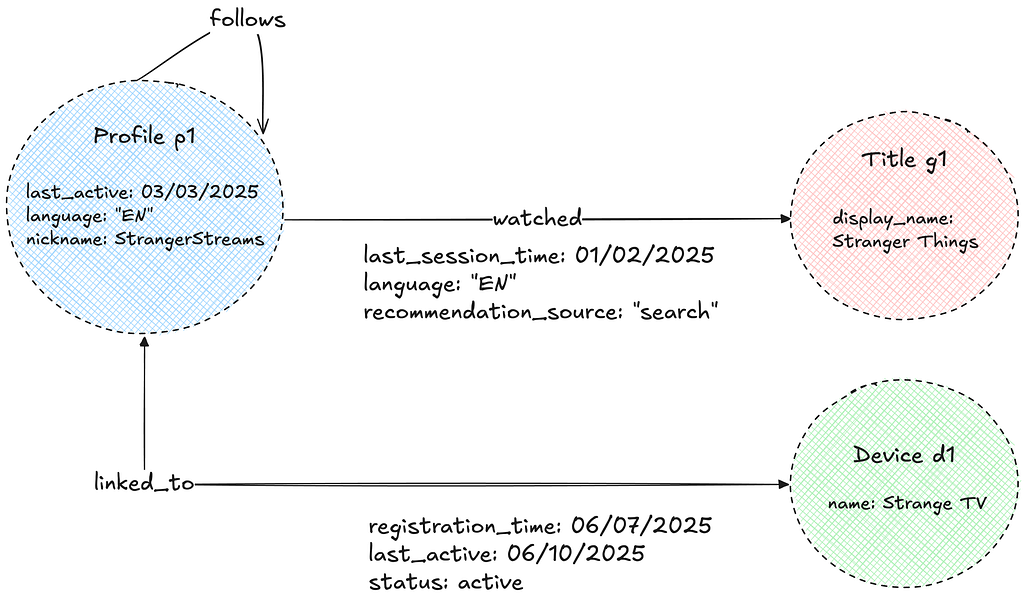
The Abstraction uses the Property Graph model to store its data. The graph consists of nodes and edges of various types, each with associated properties. These properties are strongly typed to enable efficient filtering and ensure consistent data exports. For semantic reasons, edges can be either unidirectional or bidirectional.
Namespaces
The Abstraction separates data into isolated units called “namespaces.” Each namespace is associated with a physical storage layer, as configured in the Data Gateway Control Plane, and can be deployed on either dedicated or shared hardware. The optimal, most cost-effective hardware configuration is determined by our provisioning automation, based on user-provided requirements such as throughput, latency, dataset size, and workload criticality. For more details on this topic, see this talk given by our stunning colleague Joey Lynch at AWS re:Invent.
Graph Schema
Each namespace is further associated with an explicit graph schema configured in the Control Plane. The graph schema defines node and edge types, allowed properties, permitted relationships, and directions.
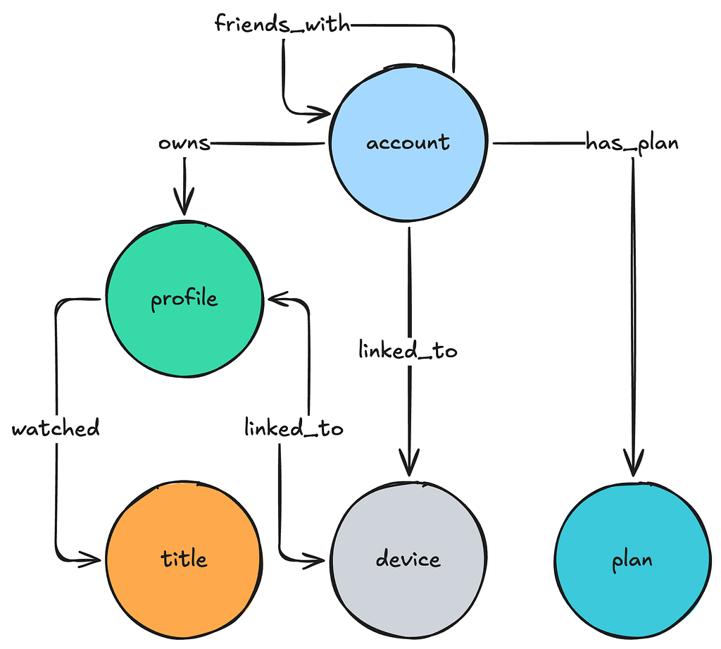
The Graph schema is implemented as a collection of edge mappings that describe the nature of the relationship between given node types.
{
  "edgeConfig": {
    "edgeMappings": [
      {
        "edgeMappingKey": {
          "fromNodeType": "account",
          "edgeType": "owns",
          "toNodeType": "profile"
        },
        "directionType": "UNIDIRECTIONAL"
      },
      {
        "edgeMappingKey": {
          "fromNodeType": "profile",
          "edgeType": "linked_to",
          "toNodeType": "device"
        },
        "directionType": "BIDIRECTIONAL"
      }
    ]
  }
}
Edge mappings are further extended with specification of property schema that consists of allowed property names and their type specification:
{
   "edgeMappingKey":{
      "fromNodeType":"profile",
      "edgeType":"linked_to",
      "toNodeType":"device"
   },
   "propertySchema":{
      "propertyMappings":[
         { "propertyKey":"registration_time", "propertyValueType":"TIMESTAMP" },
         { "propertyKey":"status", "propertyValueType":"STRING" }
      ]
   }
}
The Abstraction servers load this schema on startup and build an in-memory metadata graph of possible relationships, enabling several key optimizations:
- Data Quality: The Abstraction rejects non-conforming nodes, edges, and properties during writes, ensuring high data quality and consistent exports.
- Query Planning: The Abstraction uses the schema to quickly construct the possible traversal paths the service should take to answer a given user query.
- Deduplication of Traversed Edges: For bidirectional traversals on edges between the same node type, the schema helps avoid redundant processing by deduplicating traversed paths.
- Eliminating Traversal paths: For a given user query, the Abstraction removes traversal paths associated with impossible relationships, as well as those where filters or property types are incompatible.
Further, the Abstraction servers periodically poll the schema from the Data Gateway Control Plane in order to keep it updated with user changes. Looking ahead, we plan to leverage the graph schema for additional improvements, such as:
- Minimizing Query Fanout: By using edge cardinality within edge mappings, we aim to select the most efficient traversal paths and minimize query fanout.
- Improved Developer Experience: The schema will support generating a type-safe data access layer and enhance the Gremlin-like API with schema awareness.
Next, let’s look at how this data is organized in a real-time index within the KV Abstraction.
Real-Time Index: Key-Value Storage
Before we discuss how the data is organized into graph indexes, let’s discuss how KV organizes data within namespaces and provides idempotency guarantees:
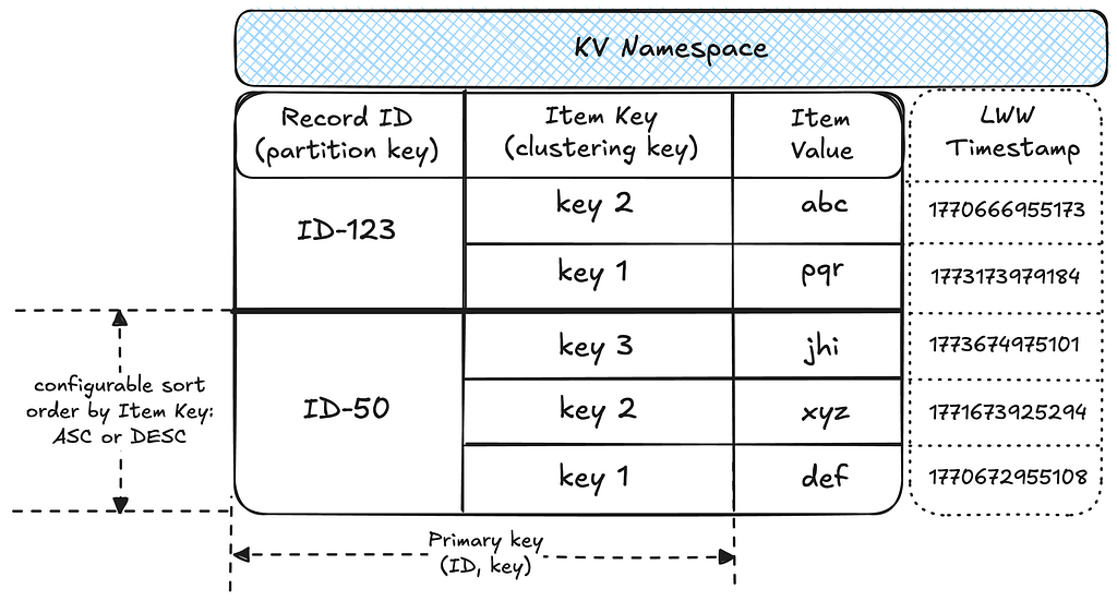
- Data partitioning: A namespace is associated with a table in the underlying storage layer. Within the table, data is partitioned into records by unique IDs, with each record holding multiple sorted items as key-value pairs. This structure effectively makes each namespace a map of sorted maps, providing flexibility for diverse access patterns.
- Idempotency: Writes to a given ID and key are idempotent, enabling request hedging and safe retries. The idempotency token contains a timestamp, which KV uses to enforce Last-Write-Wins (LWW) semantics at the storage layer.
We use the KV as the underlying storage for all real-time graph indices on nodes and edges. For more on Netflix’s Key-Value Abstraction, see this excellent post published by our KeyValue team.
Node Storage
The two-tiered partitioning strategy works well for node storage. Each node type is isolated within its own KV namespace, which stores all the properties for nodes of that type.
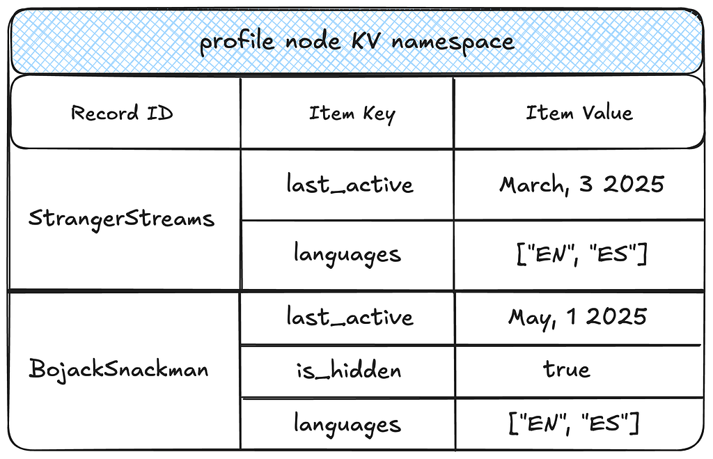
This storage format enables several efficient access patterns for nodes:
- Efficient reads: A given node and all its properties are fetched in a single partition lookup, achieving single-digit millisecond latency.
- Property selection pushdown: Target property keys are pushed down to the KV layer, reducing the amount of data fetched and further decreasing latencies and network overhead.
- Property filtering pushdown: Property keys and values can be efficiently filtered at the KV layer.
- Efficient exports: This model supports highly parallelized node exports by node type.
Edge Storage
Links and Property Index
Edges utilize two distinct types of indexes: one exclusively for the edge connections (links), and one for edge properties.
The Edge links are arranged as an adjacency list mapping source nodes to their connected neighbors.
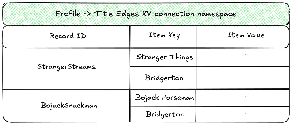
The Edge Property index stores information about properties of every edge.

Separating edge links from their properties brings several benefits, but also introduces a key trade-off:
Benefits:
- Efficient property upserts: Allows individual properties to be upserted over time without needing to read the entire property set for an edge.
- Wide row prevention: Decoupling edge links from their properties prevents large partitions in databases like Cassandra, enabling efficient storage and low-latency reads — even for edges with millions of connections.
Trade-off:
- Non-atomic writes: Storing edges across multiple namespaces means that writes across these namespaces are not atomic. We’ll discuss how this is addressed in the Consistency Enforcement section.
Forward and Reverse Indexes
Additionally, edge indexes are separated into forward and reverse indexes to support traversals in either direction. The illustration below shows an example of the reverse index counterpart for the links namespace shown above.
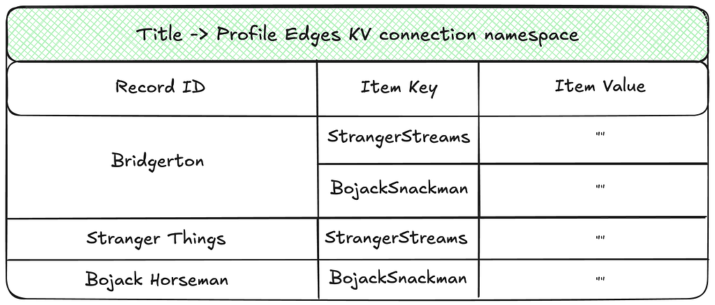
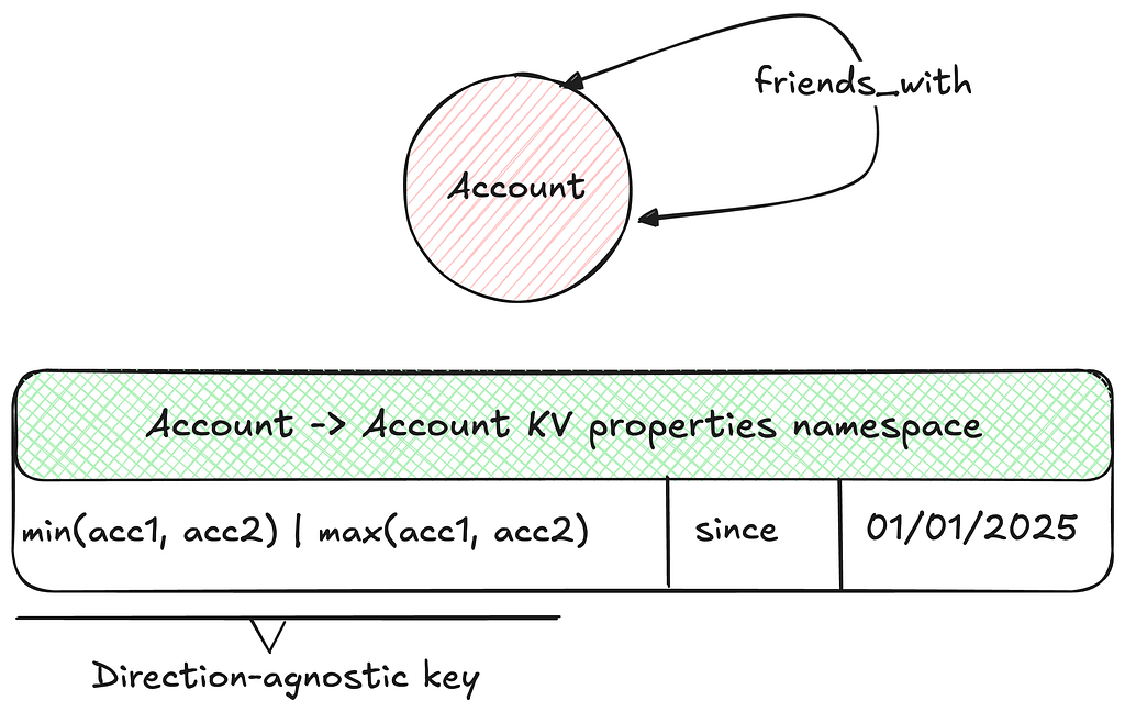
To ensure consistent record identifiers when updating edge properties in either direction, the Abstraction lexicographically sorts and concatenates the source and destination node IDs to create a direction-agnostic identifier for property storage. This ensures that properties can be accessed or mutated in a single database call regardless of the direction specified in the request.
This storage format enables several efficient access patterns:
- Point Reads: Given an edge id, all properties can be fetched in a single partition lookup on the properties index.
- Range Reads: Given a source node, a range read on a partition in the links index can efficiently return all edges. Depending on the desired direction, the Abstraction can target the forward or reverse index.
- Property Filtering: Properties are fetched only for the links that match the record or page limit criteria, minimizing the data exchanged over the network.
- Sort Orders: By default, edge links are sorted lexicographically by their target node. To support fetching the latest connections, the Abstraction retrieves target edge links in memory, sorts them by their last-write time, and returns the results. In order to ensure optimal performance without exerting too much memory pressure, we aim to limit the number of edges per source node within the system.
Next, let’s explore the caching strategies used by the Abstraction.
Caching Strategies in Graph Abstraction
Although the Graph Abstraction already provides efficient reads and writes to durable storage, caching remains critical for the stability and performance of any graph datastore for two key reasons:
- Write amplification: A single write on the fronting service can result in multiple writes to the backing durable storage due to the use of multiple indexes. Whenever possible, it’s best to avoid unnecessary writes — for example, by not writing an edge link that already exists.
- Read amplification: A single traversal request on the fronting service may translate into thousands of fetch operations on the backend, especially for highly interconnected graphs.
To address these challenges, the Graph Abstraction employs two distinct caching strategies.
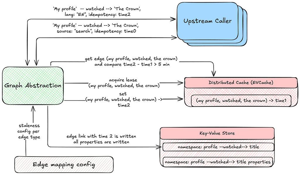
Write-aside Caching of Edge Links
An edge link contains no additional information beyond the link itself and its last-write timestamp. To reduce write amplification on durable storage, we cache edge links for short durations, helping to avoid writing a link that already exists. This mechanism is balanced with configurable TTL windows, cache invalidation on deletes, and lease acquisitions with exponential backoff. These strategies provide the necessary consistency guarantees while still allowing the last-write timestamp to be refreshed according to the predefined staleness.
Read-aside Caching of Properties
To reduce read amplification on the durable store, the Graph Abstraction leverages KV’s integration with EVCache. Multiple KV namespaces can share the same caching clusters for cost efficiency. The Abstraction first fetches data from durable storage, while subsequent reads are served from the cache. Caching is applied at both the record and item levels, benefiting all graph objects.
Graph Abstraction employs two invalidation strategies, selected based on write throughput and consistency requirements:
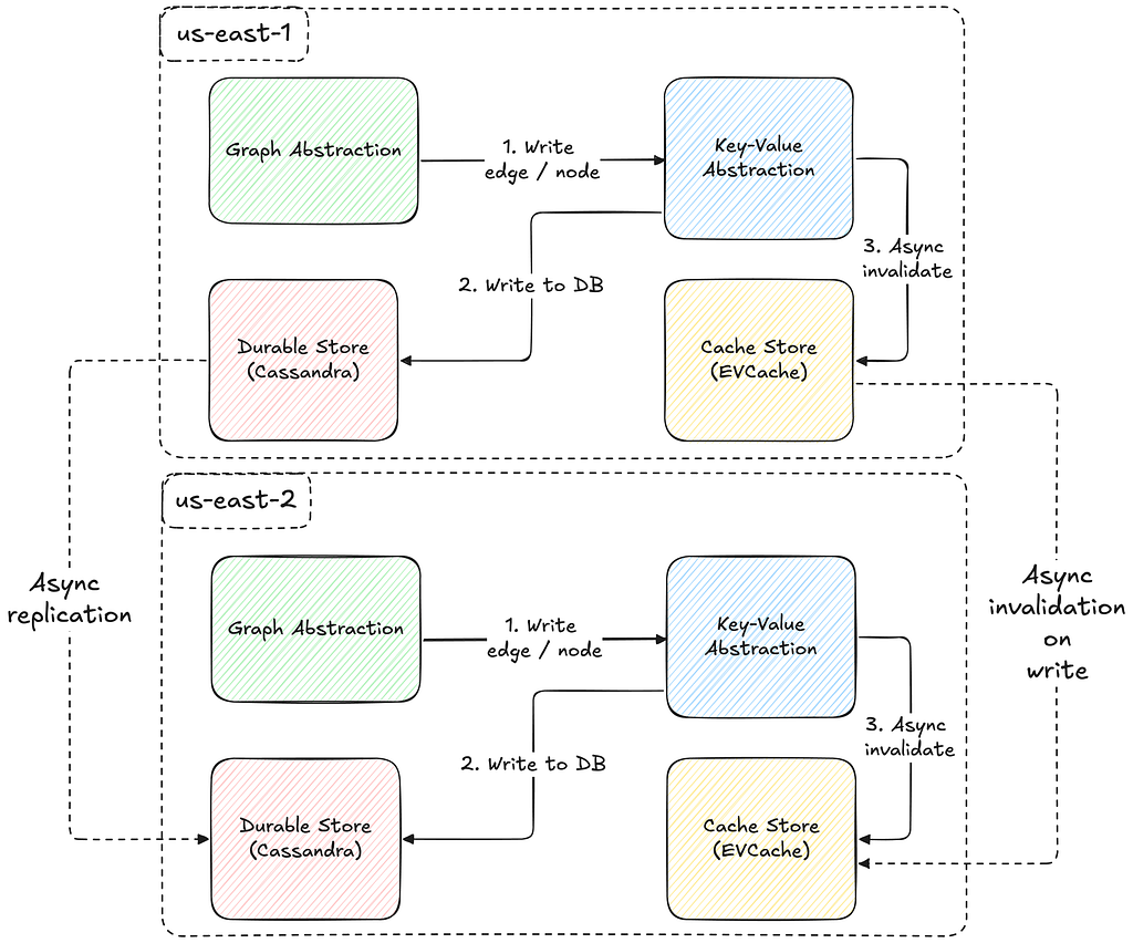
- Invalidation on write: Both record and item caches are invalidated with every write, ensuring consistency across regions. This strategy is ideal for graphs that change infrequently and cannot tolerate data staleness, but comes with the tradeoff of pushing a higher throughput on the cache.
- TTL-driven invalidation: Cache entries are invalidated only when their TTL expires. This approach works best for frequently modified objects that can tolerate some staleness.
Work In Progress: Write-Through Caching
We are also developing a write-through caching strategy designed to store most of the data required by the Abstraction during traversals. This caching mechanism can organize indexes by different sort orders (e.g., sorting data by last-write timestamp), at the cost of increased memory consumption. Stay tuned for more details on this approach.
Next, let’s examine the consistency guarantees in Graph Abstraction and how they are enforced for both reads and writes.
Consistency Enforcement
Enforcing data consistency in Graph Abstraction poses several challenges. The connected nature of the data, low-latency API requirements, and the need to handle intermittent failures have led to design choices that enforce strict eventual consistency across multiple regions.
Entropy Repair
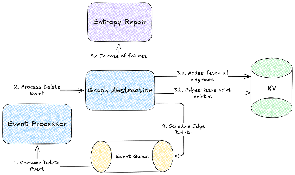
Each write in the Abstraction persists data for both inward and outward indices in parallel to support high throughput. Further, each write happens on multiple KV namespaces. To prevent inconsistencies or lasting entropy from failures in any operation, the Abstraction uses a robust retry mechanism using Kafka:

Node Deletions
Deleting nodes in a highly connected graph is more complex than simply removing a KV record as each node may have thousands of connected edges that must be handled to maintain graph integrity. Further, synchronously deleting all such connections would introduce unacceptable latency for the Abstraction callers.
The Abstraction employs an asynchronous deletion strategy to manage this issue. The consequence of this approach, however, is that the observed mutated state is only eventually consistent. Further, to ensure correctness of asynchronous deletes during concurrent updates, the Last-Write-Wins (LWW) conflict resolution mechanism is essential.
Global Replication
The consistency guarantees of Graph Abstraction are shaped by its multi-region availability. As illustrated in the diagram below, both the caching layer and durable storage replicate data asynchronously across regions, resulting in an eventually consistent system.
Now that we’ve covered storing the real-time graph index, let’s see how it enables graph traversals.
Graph Traversals
The Abstraction provides a custom gRPC traversal API, inspired by Gremlin, which enables exploration of the distributed graph by letting users chain traversals, apply filter criteria, sort results, limit results, and more.
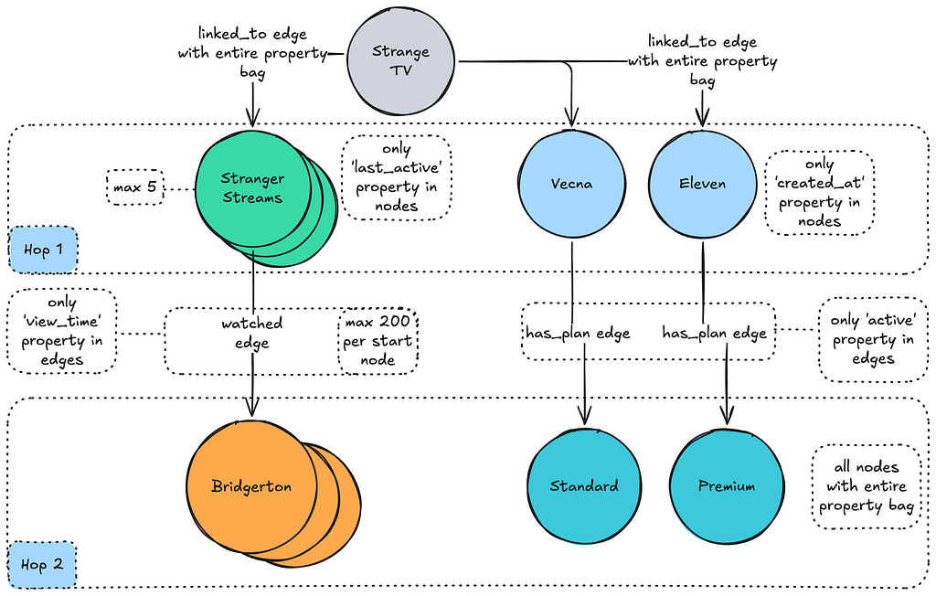
Let’s explore a hypothetical scenario where the Abstraction is used to recommend shows to users on a shared device, by considering the duration of the most recent viewing session for each show across all profiles and accounts associated with that device:
TraversalRequest.newBuilder()
  .setNamespace("<graph-namespace>")
  .setTraversalQuery(
     TraversalQuery.newBuilder()
       // Given id of the 'device' node type.
       .setStartNode(node("device", "my-device-id"))
       .setTraversal(
          Traversal.newBuilder()
            // fetch the first 5 connections
            .setEdgeLimit(5)
            .setDirectionTraversal(
               DirectionTraversal.newBuilder()
                  // traverse in the IN direction
                  .setDirection(IN)
                  // minimize data exchange: only interested in certain properties
                  .addNodePropertiesSelections(propSelection("account", "created_at"))
                  .addNodePropertiesSelections(propSelection("profile", "last_active"))
                  .setDirectionFilter(
                     DirectionFilter.newBuilder()
                       // only interested in certain connected types
                       .setTypeMatchingStrategy(EXCLUDE_NON_TARGETED)
                       .addAllNodeFilters(typeFilters("account", "profile"))))
            // chain traversals to the intermediate result
            .addNextTraversals(
               Traversal.newBuilder()
                 .setOrder(LATEST)
                 // limit to 200 connections for the 2nd hop
                 .setEdgeLimit(200)
                 .setDirectionTraversal(
                    DirectionTraversal.newBuilder()
                      // now traverse in the OUT direction
                      .setDirection(OUT)
                      .addEdgePropertiesSelections(propSelection("watched", "view_time"))
                      .addEdgePropertiesSelections(propSelection("has_plan", "active"))
                      .setDirectionFilter(
                         DirectionFilter.newBuilder()
                           .setTypeMatchingStrategy(EXCLUDE_NON_TARGETED)
                           .addAllNodeFilters(typeFilters("title", "plan")))))))
  .build();
And let’s visualize the intended results set produced by the request above:
We’ll explore the design and implementation of traversal planning and execution, along with different traversal types, in the Part II of this blog series.
Now let’s look at the performance metrics of Graph Abstraction based on current production use cases.
Real World Performance
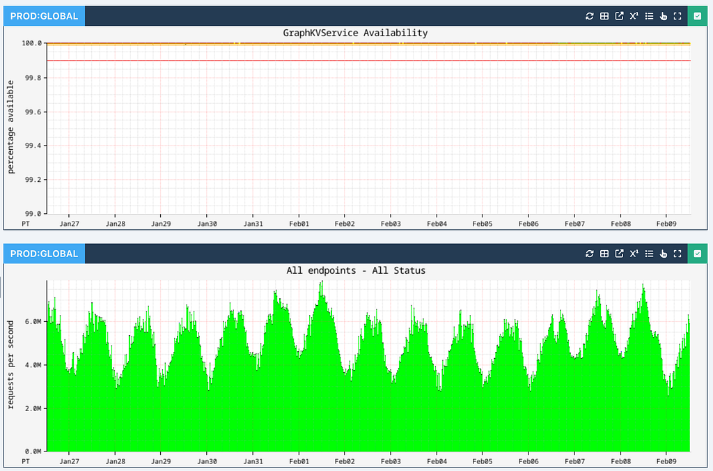
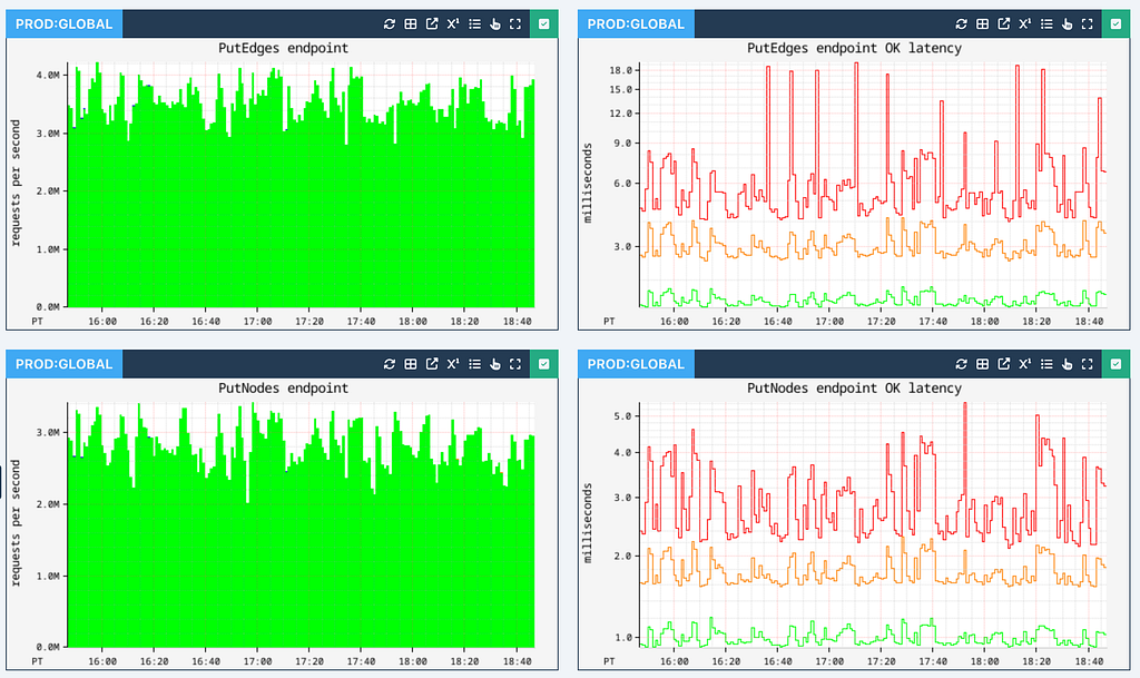
Across all applications at Netflix, Graph Abstraction ensures high availability while processing up to 10 million operations per second across all writes, individual edge / node reads and traversals at peak hours:
Edge and node persistence achieve single-digit millisecond latencies (p99 shown in red, p90 shown in orange, and p50 shown in green):
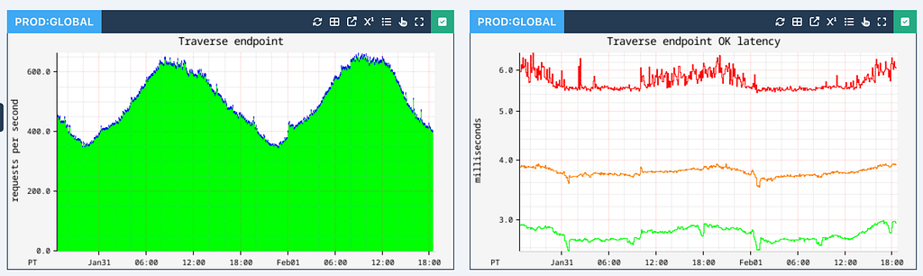
Traversal performance depends on the number of hops, the edge fanout at each stage, and associated filters and sort orders. We parallelize work as much as possible to reduce latencies. Typically 1-hop traversals are executed with single-digit millisecond latency:
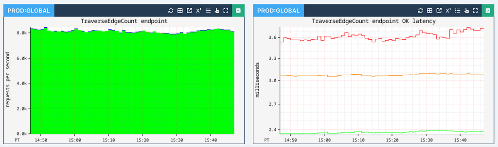
We also support a Count API that performs counting traversals at a very high rate with similar latencies, which we will cover in Part II of this series:
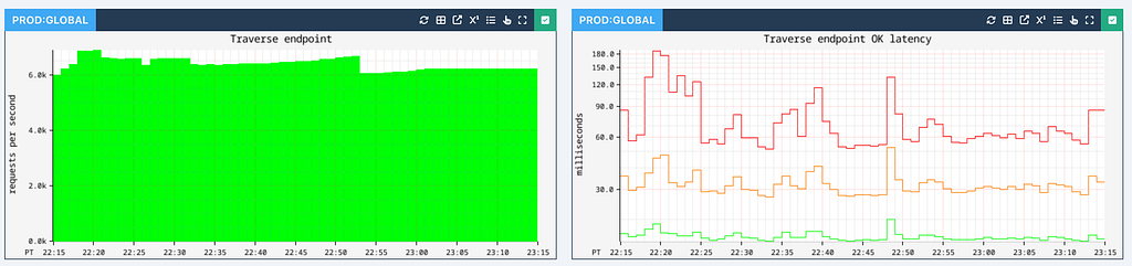
Currently, the RDG is powered by 2-hop traversals with a higher degree of fan-out. While these operations can reach upwards of 100 ms in latency, the 90th percentile (p90) latency remains under 50ms.
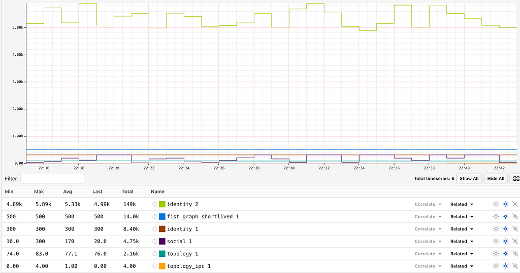
We track the average and max edge fanout at different depths to give us insights into the traversal performance for different graph datasets.

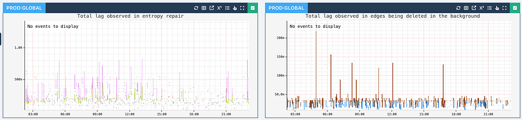
Asynchronous operations such as node deletions can be slightly latent, but typically perform with sub-second latency:
At the moment, we are storing close to 650 TB of data globally across all our graph datasets.

Conclusion
As Netflix scales further into new verticals such as live content, games, and ads, Graph Abstraction will remain crucial for uncovering and leveraging rich connections — while continuing to support a high throughput and availability at low latencies.
Stay tuned for Part II of this blog series, where we’ll explore the implementation of graph traversals, counting and constraint mechanisms.
In Part III, we’ll take a closer look at the temporal index implementation and its integration with the Time Series Abstraction.
Acknowledgments
Special thanks to our stunning colleagues who contributed to Graph Abstraction’s success: Kaidan Fullerton, Joey Lynch, Sudhesh Suresh, Vinay Chella, Sumanth Pasupuleti, Vidhya Arvind, Raj Ummadisetty, Jordan West, Chris Lohfink, Joe Lee, Jingxi Huang, Jessica Walton, Prudhviraj Karumanchi, Akashdeep Goel, Sriram Rangarajan, Chris Van Vlack, Christopher Gray, Luis Medina, Ajit Koti, Mohidul Abedin.

High-Throughput Graph Abstraction at Netflix: Part I was originally published in Netflix TechBlog on Medium, where people are continuing the conversation by highlighting and responding to this story.

