Tag Archives: Platform Engineering

In-House LLM Serving at Netflix

Post Syndicated from Netflix Technology Blog original https://netflixtechblog.com/in-house-llm-serving-at-netflix-a5a8e799ea2c

By AI Platform’s Model Runtime team and Inference team

Introduction

Most organizations consume LLMs through hosted APIs. Netflix went further — we run the full stack ourselves, from model deployment through inference, inside our existing production environment rather than a separate ML silo. Some of those decisions weren’t obvious, and a few revealed their trade-offs only under production load.

This post focuses on the choices where alternatives were seriously considered: engine selection, model packaging, API surface design, deployment strategy, and output constraints enforcement. The goal is to share not just what was built, but why — and what production revealed that the design phase didn’t anticipate.

Architecture Overview

Member-scale ML at Netflix is fronted by a unified JVM-based serving system that handles the end-to-end flow for downstream consumers: routing and A/B test logic, candidate generation, feature fetching, inference, post-processing, and logging at each stage. Both real-time and cached batch paths are supported. Figure 1 shows the two ways callers reach inference today: the gRPC path through this serving system and a direct HTTP path used by newer LLM-driven applications.

Where inference runs depends on the model. Small CPU models run in-process, avoiding remote-call overhead. Larger models need GPUs — the serving system handles pre- and post-processing locally but delegates inference to a remote service, Model Scoring Service (MSS). MSS is the shared inference backend, supporting XGBoost, TensorFlow, PyTorch, and LLMs behind a unified interface, with NVIDIA Triton Inference Server underneath managing model loading, batching, and GPU scheduling.

On top of Triton sits a Java control plane that handles deployment, versioning, health checking, autoscaling, and multi-region rollout. Model authors package their artifacts and configure the deployment; the control plane provisions GPU instances, configures Triton, and orchestrates zero-downtime upgrades.
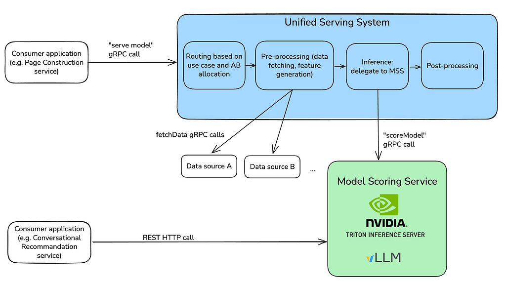
Figure 1. Serving Architecture Overview

Design Decisions and Implementation

Four decisions shape this platform — engine, packaging, API surface, and rollout — presented in dependency order, since each one constrains the next.

vLLM as the Paved-Path Engine

The platform was originally built on TensorRT-LLM, a performant inference engine at the time and already integrated with Triton — the compute backend in use within MSS.

By summer 2025, two things had shifted: open-source engines had largely closed the performance gap with specialized stacks, and our workload mix had broadened to include embedding generation, prefill-only inference for ranking and retrieval, autoregressive decoding, and custom models with non-trivial per-step constraint logic. We re-benchmarked against this mix and selected vLLM as our paved-path engine on operational fit:

  • Loads custom model architectures without a multi-step compilation pipeline — faster iteration on non-standard models.
  • Extensibility hooks for custom decoding logic — necessary for the constrained-decoding work described later.
  • Debuggability — easier to inspect failures and intermediate state than with a compiled engine in earlier TensorRT-LLM.
  • Familiarity — many ML practitioners were already using vLLM in research, which cut the research-to-production handoff cost.

Integrating vLLM into Triton

With vLLM picked, the next decision was how to package models for it. Triton supports two ways, and the choice has significant implications for maintainability — specifically, how tightly model artifacts are coupled to frontend upgrades.

  • Python backend. The author defines explicit input/output tensor specs at packaging time. These specs are frozen in the artifact and must match what the third-party vendor’s frontend’s request builder expects, so every frontend upgrade that touches I/O specs requires a coordinated change to packaging code; otherwise, requests fail at runtime.
  • vLLM backend. The artifact is just a JSON config pointing to the model weights and tokenizer. Triton’s vLLM backend reads this config and generates I/O tensor specs dynamically at deployment time — the author never defines them. Models and frontend evolve independently.

The vLLM backend is the architecturally correct default. Two things bit us in production:

  • Triton/vLLM version mismatch. Triton’s vLLM backend is compiled against a specific vLLM API surface. When the two drift — for example, Triton 25.09 importing vllm.engine.metrics, a module removed in vLLM 0.11.2 — the backend fails to load entirely. The platform has to pin compatible versions when baking the service image, and prevent model authors from overriding the vLLM version at packaging time.
  • Custom model logic. The vLLM backend expects a standard HuggingFace-compatible model and handles the full inference lifecycle. Models needing custom preprocessing, postprocessing, or non-standard execution — ensemble pipelines, custom tokenization — must use the Python backend, which gives full control over execute(). This escape hatch will likely remain necessary for a subset of models.

Ecosystem-Compatible HTTP Frontend

With engine and packaging settled, the next question is how callers reach the system. A key design goal of our system was that LLM models should NOT be special snowflakes. Every model — XGBoost ensemble or large-scale LLMs — is scored via the same gRPC call, so we reuse the same client libraries, health checking, and deployment pipelines. Given that the OpenAI-compatible API interface has become the de facto interface for the LLM ecosystem — inference engines, orchestration frameworks, evaluation tools, and client libraries all speak it — so we expose the OpenAI-compatible API as an additional frontend alongside gRPC.

The payoff shows up in the experimentation-to-production path: graduating from a hosted model to a fine-tuned self-hosted one — for quality, latency, cost, or data privacy — is nearly seamless. Same API, minimal code changes.

Behind the API, the implementation reuses NVIDIA’s Triton OpenAI-compatible frontend. It starts an embedded Triton server, wraps it in a TritonLLMEngine that converts request schemas into Triton inference requests, and serves responses through FastAPI. KServe HTTP/gRPC frontends are enabled alongside, so the same Triton instance remains accessible to the Java control plane over gRPC. Adopting Triton’s frontend directly exposed one gap: response_format — accepted by the schema — was silently dropped before reaching vLLM, so that a caller requesting JSON output proceeded without guided decoding constraints and could receive malformed JSON with no error surfaced by the platform. We git-subtreed and patched the frontend to translate response_format into vLLM’s guided decoding parameters at request time.

Deployment Strategies

With API surface and engine in place, the question that remains is how new versions roll out without dropping requests. GPU deployments take longer to bring up than CPU services, and the I/O schema may change between model versions — adding a coordination problem on top. The platform offers two strategies:

  • Red-Black deploys a new version alongside the current one. Once the new instance passes health checks, traffic shifts in phases — the new version scales up while the old scales down at the same rate. If any step fails, the system triggers an atomic rollback. Red-Black is the right choice when the model interface is stable. Production revealed a coordination gap when a new version requires an I/O schema change (e.g., new tensor dimensions): the upstream consumer can’t update its config until the new model is fully live, so it inevitably sends “old” requests to a “new” deployment during the migration window, and those fail.
  • Versioned solves that gap by maintaining an independent deployment for every (modelId, modelVersion) pair. Multiple versions serve simultaneously, decoupling model deployment from consumer updates: the consumer waits for the new version to be fully ready before switching its config, while the old version keeps serving legacy traffic. The platform cleans up older deployments after inactivity but always preserves the latest. The trade-off is a temporary increase in GPU cost during the transition overlap.

We recommend embedding variable configurations (e.g., tensor shapes) directly into the inference model to make it version-agnostic, so it can use the cheaper Red-Black path. Versioned is reserved for the rare cases where a breaking interface change is unavoidable.

Operational Notes

Beyond those four decisions, two operational details are worth flagging — both hit production gaps the design phase didn’t anticipate.

Boot sequence

Bringing a vLLM-on-Triton instance up involves several coordinated steps before the gRPC port opens. Two are non-routine.

  • Model caching. Downloading large LLMs directly from S3 or Hugging Face at startup is slow enough to inflate cold-start latency past what schedulers tolerate. We materialize models on Amazon FSx at the time of model announcement, so warm starts hit a high-performance file system instead of object storage.
  • Embedded vs standalone Triton. When consumers need the OpenAI-compatible API, Triton runs as an embedded server inside the OpenAI-compatible frontend process; otherwise, it runs standalone. This is configured per-deployment at packaging time.

The rest of the boot sequence is mechanical: extracting the model package, installing custom vLLM plugins via Python entry_points, cleaning the Prometheus multiprocess directory, and gating the gRPC port until the engine is ready.

Unified metrics endpoint

The Prometheus cleanup above hints at a wider observability gap. vLLM writes metrics to PROMETHEUS_MULTIPROC_DIR as .db files; Triton reports server-level metrics through its own Prometheus endpoint. Neither is aware of the other, and Triton’s built-in bridge surfaces only 9 of 40+ vLLM metrics — missing critical ones like token throughput, KV cache utilization, and prefix cache hit rates.

We added a lightweight HTTP proxy that merges both into a single /metrics endpoint: it fetches Triton metrics via HTTP, reads vLLM metrics from disk using Prometheus’s MultiProcessCollector, and returns the combined output. Existing dashboards and alerts work without modification.

Deep-Dive: Constrained Decoding at Scale

Some Netflix production workloads rely heavily on fine-grained control over token generation. Rather than applying business logic after inference — paying for invalid generations, then retrying or repairing — we push constraints inside the decode loop, so the model generates outputs that are compliant by construction. We implement this via vLLM’s custom logits processor interface, modeling each constraint as a state machine that evolves with the generated token history and emits token-eligibility masks at each step. Each request gets its own configured processor, since different requests apply different rules.

Getting this to scale ran across two engine versions: we initially deployed on vLLM V0 (V1 had feature gaps), then migrated to V1 in Q4 2025 once it matured. The two subsections that follow are the before-and-after.

Why the first implementation didn’t scale

Our initial pure-Python implementation worked functionally but hit a scaling bottleneck. In vLLM V0, custom logits processors run per-request: the GPU produces logits for the whole batch, the CPU copies them across and waits for the transfer, and then constraint logic runs sequentially for each request — sequentially because the GIL prevents Python from parallelizing the per-request work. CPU time in logit processing therefore grows linearly with batch size, hitting tail latencies. End-to-end latency becomes CPU-bound even though the model’s forward pass is batched efficiently on GPU. It’s a bottleneck invisible in single-request benchmarks that only surfaces under realistic concurrency. Figure 2 makes the serial pattern visible.
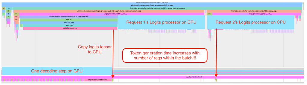
Figure 2: Logits processor serial execution on CPU with vLLM V0

vLLM V1 enabled a batch-level design

The structural fix arrived in vLLM V1, which moved logits processing to batch level. We rewrote our custom processor to operate on batch-level data structures, computing masks across many requests together, and reimplemented the hot path in C++ with multi-threading to step around the GIL. The V1 API requires explicit tracking of batch membership changes via update_state(batch_update) — more complex than V0’s per-request interface, but necessary to maintain correct state in a dynamically evolving batch. Figure 3 shows logits processing time staying flat as batch size grows.
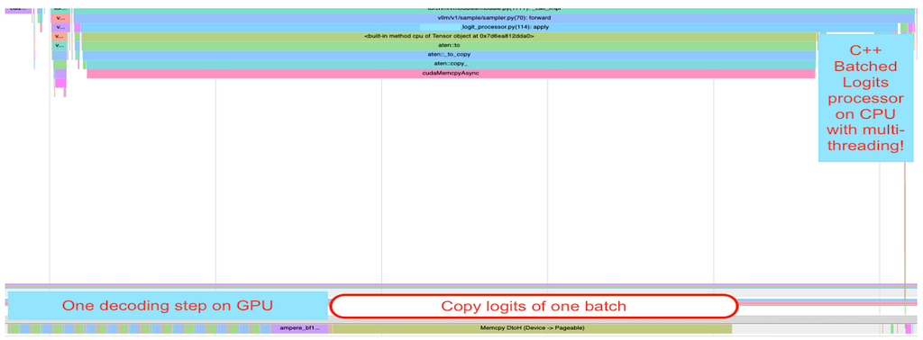
Figure 3: Batched logits processor execution on CPU with vLLM V1

Operational hardening

Now, performance was no longer the bottleneck. But stateful constraint logic in the decode loop introduced two issues the design phase didn’t anticipate:

  • Partial prefills. V1 performs chunked prefilling, so a request can be prefilled over multiple engine steps. BatchUpdate lacks the granularity to tell whether a request was fully or only partially prefilled, so we added internal tracking.
  • Preemption. Under memory pressure, vLLM may evict a partially completed request’s KV cache and reschedule it later with a different prompt and output token list. This breaks the state machine’s assumption that the output token list grows monotonically. We detect when the token history shrinks between decode steps, reset the state machine, and reinitialize from the new prompt.

Wrap up

We set out to build an LLM serving platform for broad production ML requirements — low latency, deep customization, and integration with existing infrastructure. The result is a system on vLLM and Triton, unified behind a consistent API, designed to give ML practitioners a fast path from experimentation to production.

The lessons were often in the details — version pinning, silent API gaps, packaging trade-offs — but addressing them has made the platform meaningfully more robust and the developer experience smoother. Next investments reflect where we expect friction:

  • System prompt compression to reduce prompt length without sacrificing quality.
  • Asynchronous scheduling of vLLM V1.
  • Vectorized logits processors that run as fused GPU kernels instead of CPU code.
  • Lower-precision model variants to decrease memory footprint and increase throughput.

We’ll continue working closely with the open-source community as this space evolves.

Contributions

This system is the result of close collaboration and contributions from many teams within the AI Platform org at Netflix. In particular, Liping Peng designed and developed the model packaging workflow and drove the integration of Triton and vLLM with MSS to enable a unified pathway for serving LLMs. Hakan Baba, Nicolas Hortiguera, and ZQ Zhang led GPU capacity planning, system performance tuning, application integration and observability, as well as A/B test readiness and operational excellence efforts for all production models. Santino Ramos enabled vLLM for production models and optimized constrained decoding performance. Binh Tang developed the initial version of custom model serving and benchmarked different LLM serving frameworks. Lanxi Huang and Daneo Zhang built the serving development tools to enable user self-service. Lingyi Liu drove the overall system architecture and core technical decisions. Abhishek Agrawal and Shaojing Li provide management leadership to ensure alignment, prioritization and execution.

Acknowledgements

This work heavily leverages open-source ML libraries, such as Triton, vLLM and PyTorch, etc. We’re especially grateful to the teams and contributors from the community. We also thank our partner teams in Netflix AI for Member Systems for their close collaborations and innovation on the modeling side.


In-House LLM Serving at Netflix was originally published in Netflix TechBlog on Medium, where people are continuing the conversation by highlighting and responding to this story.
From Silos to Service Topology: Why Netflix Built a Real-Time Service Map

Post Syndicated from Netflix Technology Blog original https://netflixtechblog.com/from-silos-to-service-topology-why-netflix-built-a-real-time-service-map-0165ba13a7bc

By Parth Jain, Rakesh Sukumar, Yingwu Zhao, Renzo Sanchez & Nathan Fisher
How we built a living map of our distributed infrastructure to help engineers understand dependencies, troubleshoot faster, and keep Netflix running smoothly for our members around the world.

The Puzzle with a Thousand Pieces

Picture this: It’s 3am, and an engineer gets paged. One of our critical services is showing elevated error rates. Members trying to watch their favorite films and series are seeing degraded experiences. The clock is ticking.

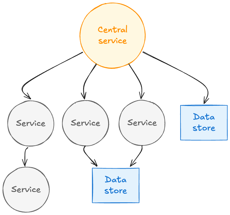
A central service node connected to multiple downstream services and data stores, illustrating the tangled dependency graph engineers must navigate without a service topology map.
A single service at the center of a web of dependencies — services, data stores, and call chains branching in every direction. Without a unified map, engineers have to reason about this structure from memory and scattered signals.

In a system with thousands of microservices supporting our entertainment experience for members worldwide, answering these questions quickly can mean the difference between a minor blip and a major incident.

We kept hearing variations of this story from engineers across Netflix. The tooling gap was clear: we had plenty of signals, but no unified way to understand how everything connected.

The Three Questions Every Engineer Asks

When troubleshooting distributed systems, engineers fundamentally need to understand relationships:

Which services depend on each other? Not just theoretical dependencies from configuration files or architecture diagrams, but actual runtime connections based on real traffic.

What’s the blast radius? When something breaks or needs to go down for maintenance, what else will be affected? Which teams need to be notified?

Where’s the source? Is my problem caused by an upstream issue, or am I the root cause that’s cascading to others?

Traditional observability tools show fragments of this picture. Metrics show symptoms and performance characteristics. Logs show individual service behavior. Traces show single request flows through the system. But none of them show the complete map of how everything connects — the steady-state topology of dependencies that forms the backbone of our distributed architecture.

For an engineer at 3am, having to mentally stitch together information from multiple tools is slow, error-prone, and stressful. We needed something better: a unified view of service dependencies — a map showing how everything connects — with easy navigation to the detailed signals when you need to dig deeper.

Why This Matters More Than Ever

Netflix runs on thousands of microservices working together to deliver entertainment to our members. When you press play on your favorite series, that single action triggers a cascade of service-to-service calls — authentication, recommendations tailored to your tastes, video encoding selection, playback optimization, and more.

This architecture gives us tremendous flexibility and allows hundreds of engineering teams to innovate independently. But it also creates fundamental observability challenges.

And these challenges were growing. New initiatives like our Live programming and Ads-supported plans require even more sophisticated monitoring and faster troubleshooting. Live events can’t wait for lengthy incident investigations. The scale and real-time nature of these systems demanded better tooling.

We analyzed thousands of support requests from our engineers over a four-year period. The patterns were consistent:

  • “What are my upstream and downstream dependencies?”
  • “Is this failure in my service, or is something I depend on broken?”
  • “Which services will be impacted if I take this down for maintenance?”
  • “Why is this service showing as ‘Unknown’ in my metrics?”
  • “What changed in my call path recently that could explain this behavior?”

Engineers were asking dependency questions constantly. We needed to provide answers — quickly, accurately, and in real-time.

Building on What We Learned

We didn’t start from scratch. Over the years, we explored various approaches to solving this problem — from evaluating external graph databases and vendor platforms to building internal prototypes with different storage technologies and data models.

Each iteration taught us something valuable:

Real-time matters: Dependency maps that are hours old are useless in dynamic environments where services deploy multiple times per day. We needed near real-time updates.

Scale changes everything: Solutions that work at modest scale hit fundamental walls at Netflix scale. Storage systems that handle thousands of nodes struggle with our service count and traffic volume.

Integration is key: Any solution needs seamless integration with our existing observability ecosystem. Engineers shouldn’t have to learn entirely new tools or leave their existing workflows.

Data quality is critical: Incomplete or incorrect dependency information is worse than no information — it leads to wrong conclusions during incidents.

Multiple perspectives needed: We learned that no single source of dependency information tells the complete story. Network connectivity data lacks application context. Application metrics only cover instrumented services. We needed to combine multiple sources.

These lessons shaped every decision we made in building Service Topology.

What We Needed: A Living Map

We set out to build something specific: a living map of our infrastructure — one that updates in real-time as services deploy, as traffic patterns shift, as new dependencies form and old ones disappear.

The requirements were clear:

Real-time updates, not stale snapshots: In an environment where services deploy continuously, yesterday’s topology map is archaeology, not observability.

Fast queries at scale: When an engineer is troubleshooting at 3am, they can’t wait minutes for a query to return. We needed sub-second response times for traversing the call graph.

Multiple layers: Network-level connectivity doesn’t tell the whole story. We needed to see both the network layer (what’s actually talking to what) and the application layer (which APIs and endpoints are being called).

Rich context, not just connections: Knowing Service A talks to Service B isn’t enough. We needed to overlay health status, availability tiers, business domains, ownership information, and other metadata to make the information actionable.

Visual and programmatic access: Engineers needed a UI for exploration and troubleshooting. But automated systems — resilience frameworks, blast radius calculators, incident response automation — needed programmatic API access.

Our Approach: Three Sources of Truth

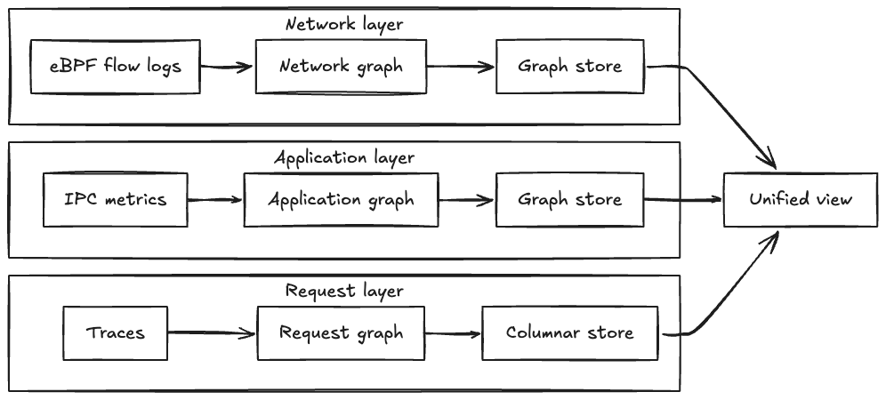
Three topology layers side by side: eBPF flow logs producing a network graph, IPC metrics producing an application graph, and distributed traces producing a request graph, all feeding into a unified view.
Three data sources produce three independent topology graphs — network, application, and request — each stored separately and queryable on their own or merged into a single unified view.

Here’s the key insight we arrived at: no single source tells the complete story.

We built Service Topology by using three complementary sources to build separate dependency graphs — one from each perspective — that can be combined into a unified view or explored independently:

Each source creates its own graph that is physically separate — the network layer in one graph database partition, the IPC layer in another partition, and the tracing layer using columnar storage optimized for analytical queries. This physical separation allows each layer to evolve independently and be queried in parallel. When users request a unified view, we execute traversal queries across all layers simultaneously and merge results, achieving sub-second response times even when combining all three layers.

Each source creates its own graph of service relationships:

1. eBPF Network Flows (Network Layer)

We capture network flow records at the kernel level using eBPF technology — information about which services are connecting to which other services over the network. This gives us ground truth about actual network-level communication.

The value: Comprehensive coverage. Every service shows up here because we’re capturing actual network traffic, regardless of whether applications are instrumented. This layer provides topology at both cluster-level (which deployment clusters are communicating) and app-level (which applications are communicating).

The limitation: Network-level information lacks application context. We know Service A connected to Service B’s IP address using a specific protocol, but not which specific API endpoint or path was called (e.g., /api/v1/users vs /api/v1/orders).

2. IPC Metrics (Application Layer)

We collect Inter-Process Communication metrics from our instrumented services. These are the metrics applications emit when they make calls to other services via gRPC, GraphQL, REST, or other protocols.

The value: Rich application context. We can see which specific endpoints were called, error rates, latency distributions, protocol details, and request/response characteristics. This layer provides app-level topology — since IPC metrics are emitted by applications, the natural granularity is application-to-application connections with endpoint details.

The limitation: Only works for instrumented services. If a service doesn’t emit IPC metrics, we won’t see its application-level calls this way.

3. End-to-End Tracing (Request Layer)

We integrate distributed tracing information that follows individual requests as they flow through our system. We aggregate traces to build a unified topology graph, but also allow engineers to overlay individual traces on the topology to see specific request flows.

The value: Shows actual request paths. Not just “Service A can call Service B,” but “Service A did call Service B as part of serving this specific member request.” This captures runtime behavior, including conditional logic and feature flags. Engineers can both see the aggregated pattern and drill into individual traces. We aggregate traces to build topology at both cluster-level and app-level, allowing engineers to view request patterns at the granularity most useful for their investigation.

The limitation: Sampling. We can’t trace every request without impacting performance, so we sample. This is excellent for understanding common flows, but may miss rarely-used code paths in the aggregated view.

Bringing It Together: Multi-Layer Architecture

Here’s what makes this powerful: we build three separate graphs — one from each source — that create different perspectives on service relationships:

  • Network graph from eBPF flows: Every connection, regardless of instrumentation
  • Application graph from IPC metrics: Rich endpoint and protocol details
  • Request graph from tracing: Actual runtime behavior and call paths

Engineers can:

  • View each graph independently to focus on a specific perspective (pure network connectivity, application-level calls, or traced request flows)
  • Combine them into a unified graph by querying multiple partitions in parallel and merging results — our system returns the union of nodes and edges from all requested layers while preserving each layer’s distinct properties

The unified view is especially powerful because:

  • Network flows ensure completeness — we don’t miss anything
  • IPC metrics provide application details — we understand the “how” and “what”
  • Tracing shows actual behavior — we see real request patterns

Each source compensates for the limitations of the others. The result is a comprehensive, accurate, and contextualized view of service dependencies that can be explored from multiple angles.

From Flows to Graph: How We Built It

Here’s the high-level architecture (we’ll dive deeper into engineering challenges in our next post):

Pipeline diagram showing data flowing from a message stream through Stage 1 initial aggregation, Stage 2 intermediary resolution, and Stage 3 persistence and enrichment into a graph database, then exposed via an API.
Flow logs travel from multi-region Kafka through three aggregation stages — initial batching, intermediary resolution, and final enrichment — before being persisted to the graph database and served via API.

Multi-Region Ingestion: We consume flow logs from Kafka across multiple AWS regions where Netflix operates. This runs continuously, processing millions of flow records as they arrive.

Distributed Processing: We use Apache Pekko Streams (a fork of Akka) to process these flows in a distributed, fault-tolerant pipeline. The system automatically partitions work across our Auto Scaling Groups to handle the volume and provides natural backpressure handling.

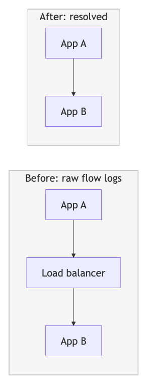
Three-Stage Distributed Aggregation: We aggregate network flows through a three-stage pipeline that solves a fundamental challenge: network flow logs only show individual network hops through intermediaries (App A → Load Balancer → App B, or App A → NAT Gateway → App B), not the true application-level connections we need (App A → App B).

Before and after diagram showing intermediary resolution: raw flow logs recording two hops from App A through a load balancer to App B are collapsed into a single direct edge from App A to App B.
Stage 2 resolves network intermediaries: raw flow logs show two separate hops (App A → Load Balancer → App B), but the resolved graph stores the direct application-to-application relationship (App A → App B).

Stage 1 performs initial aggregation from Kafka. Stage 2 applies resolution logic — identifying network intermediaries (load balancers, NAT gateways, API gateways, proxies) and combining their incoming and outgoing flows to reconstruct direct application-to-application paths. Stage 3 performs final aggregation with health status integration before graph persistence. This graduated approach also prevents hot spots by distributing load across multiple points even when specific applications or network intermediaries see 100x more traffic than others.

Graph Storage: We persist the topology in Netflix’s graph database, an abstraction layer built on top of our distributed key-value storage infrastructure. This graph database is specifically designed for high-throughput graph operations at our scale, with fast multi-hop traversal capabilities. Each of our three data sources (network flows, IPC metrics, tracing) creates a separate graph that can be queried independently or merged.

gRPC API: We expose the topology through a gRPC service that supports multi-hop traversal, filtering by availability tier and business domain, pagination for large result sets, and sub-second query response times.

The technical details of building this at Netflix scale — handling Kafka lag, managing memory and garbage collection, optimizing distributed processing, debugging reactive streams — deserve their own discussion. We learned a lot, and we’ll share those lessons in our next post.

What Engineers Can Do Now

Today, the service topology map is helping engineers across Netflix:

Visualize Dependencies: See upstream and downstream dependencies for any service, with the ability to filter by availability tier (Tier 0, Tier 1, etc.) and business domain. Choose between the unified view (combining all sources) or individual graph views (network-only, IPC-only, or trace-only) depending on what you’re investigating.

Jump to Detailed Signals: From any service in the topology, quickly navigate to logs, traces, and detailed metrics in their respective tools. No more hunting for the right service name or time window — the topology provides the context and the starting point.

Understand Blast Radius: Before taking a service down for maintenance or making significant changes, see exactly what will be impacted. Identify which teams to notify and what to monitor.

Overlay Health Status: See not just the topology, but which services in the call path are experiencing issues. This is integrated with health status tracking, so you can quickly identify if a problem you’re seeing is actually originating somewhere else.

Query Programmatically: Use our gRPC API to integrate topology information into automated systems. For example, our Platform Modernization Engineering team uses this to verify that critical Live services have proper availability tier classifications throughout their dependency chains.

Investigate Faster: During incidents, quickly identify if a failure is local or if it’s propagating from somewhere else in the call graph. Follow the failure pattern to find the root cause.

Plan Changes Confidently: Understand the impact of proposed architectural changes or service migrations before implementing them.

Time Travel Through Topology: Query what the topology looked like at specific points in the past. Understand what changed in dependencies around the time an issue started, or see how your service’s dependency footprint has evolved over time. This time-travel capability is powered by time-window aggregation — instead of storing every time slice separately, we use layer-specific aggregators that accumulate topology data across windows, allowing us to reconstruct historical views efficiently without exploding storage costs.

The Living Map: Always Current

What makes this truly useful is that it’s a living map. It’s not a static diagram drawn in a design document that goes out of date the moment it’s published. It’s continuously updated based on actual traffic:

  • When a new service starts calling an API, it appears in the topology with near real-time freshness
  • When a service stops making calls to a dependency, that edge fades from the graph
  • When services deploy and their behavior changes, the topology reflects it
  • When incidents impact service health, the status overlay updates in real-time

This means engineers can trust what they see. The map reflects reality, not someone’s idea of what the architecture should be.

The Journey Continues

We’re not done. We continue to evolve the system with new capabilities:

Change Event Overlay: We’re working to surface deployment events, configuration changes, and other mutations alongside the topology graph. Correlation becomes easier when you can see both the dependencies and what changed when.

Richer Context: As we expand coverage and integrate more signals, we continue to enrich the topology with additional endpoint-level details, protocol information, and network path context.

And looking further ahead, we’re excited about something bigger: Automated root cause analysis. Imagine an intelligent agent that continuously crawls the topology graph, correlates failures across dependencies, understands historical patterns, and surfaces likely root causes automatically. Service topology provides the knowledge graph foundation that makes this kind of intelligent automation possible.

Why This Matters for Our Members

This might seem like infrastructure — plumbing that our members never see directly. But it matters immensely to their experience.

When engineers can quickly understand dependencies and identify issues, incidents get resolved faster. When we can model blast radius before making changes, we avoid disruptions. When automated systems can query dependency information programmatically, we can build smarter, more resilient systems.

All of this translates to what matters most: our members getting to watch their favorite films and series, seamlessly, whenever they want. Whether it’s a weekend binge of a beloved show, a live sports event, or discovering something new through our recommendations tailored to their tastes — we want it to just work.

What’s Next in This Series

This is the first in a series of posts about building Service Topology at Netflix.

In our next post, we’ll pull back the curtain on the engineering challenges we faced at scale: How do you handle Kafka consumer lag when ingesting millions of flow logs per second? What happens when distributed processing meets garbage collection pauses? How do you debug reactive streams that stall under load? How do you manage hot nodes in a distributed system? We’ll share the real problems we hit in production and the solutions we developed.

In future posts, we’ll explore the lessons we learned that apply to any distributed system at scale, and where we’re heading next with time travel capabilities and Automated root cause analysis.

Acknowledgements

This post was written by Parth Jain.

Service Topology was built by Parth Jain, Rakesh Sukumar, Yingwu Zhao, Renzo Sanchez-Silva, and Nathan Fisher.

Special thanks to the many engineers across Netflix who made this possible — the Observability team who built the broader system, the graph database platform team who provided the storage foundation, and the Platform Modernization Engineering, Live, and Ads teams who provided invaluable feedback and use cases throughout development.


From Silos to Service Topology: Why Netflix Built a Real-Time Service Map was originally published in Netflix TechBlog on Medium, where people are continuing the conversation by highlighting and responding to this story.

How GitHub uses eBPF to improve deployment safety

Post Syndicated from Lawrence Gripper original https://github.blog/engineering/infrastructure/how-github-uses-ebpf-to-improve-deployment-safety/


Did you know that, at GitHub, we host all of our own source code on github.com? We do this because we’re our own biggest customer—testing out changes internally before they go to users. However, there’s one downside: If github.com were ever to go down, we wouldn’t be able to access our own source code.

This is what you’d call a very simple circular dependency: to deploy GitHub, we needed GitHub. If GitHub is down, then we wouldn’t be able to deploy something to fix it. We mitigate this by maintaining a mirror of our code for fixing forward and built assets for rolling back.

So we’re done, right? Problem solved? Nope, there are more circular dependencies to consider. For example, how do you stop a deployment script introducing a circular dependency of its own on an internal service or downloading a binary from GitHub?

When we started to design our new host-based deployment system, we evaluated some new approaches to prevent deployment code from creating circular dependencies. We found that using eBPF, we could selectively monitor and block those calls. In this blog post, we’ll take you through our findings and show how you can get started writing your own eBPF programs.

Types of circular dependencies

Let’s start by looking at the types of circular dependencies through a hypothetical scenario.

Suppose a MySQL outage occurs, which causes GitHub to be unable to serve release data from repositories. To resolve the incident, we need to roll out a configuration change to the stateful MySQL nodes that are impacted. This configuration change is applied by executing a deploy script on each node.

Now, let’s look at the different types of circular dependencies that could impact GitHub during this scenario.

  1. Direct dependency: The MySQL deploy script attempts to pull the latest release of an open source tool from GitHub. Since GitHub can’t serve the release data (due to the outage), the script can’t complete.  
Diagram showing a MySQL deploy script fails after attempting to pull the latest release of an open source tool from GitHub.
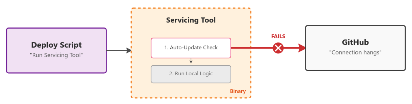
  1. Hidden dependencies: The MySQL deploy script uses a servicing tool that is already present on the machine’s disk. However, when the tool runs, it checks GitHub to see if an update is available. If it’s unable to contact GitHub (due to the outage), the script may fail or hang, depending on how the tool handles the error when checking for updates.
Diagram showing a script failing after being unable to contact GitHub (due to the outage).
  1. Transient dependencies: The MySQL deploy script calls, via an API, another internal service (for example, a migrations service), which in turn attempts to fetch the latest release of an open source tool from GitHub to use the new binary. The failure propagates back to the deploy script.
Diagram showing a MySQL deploy script calling, via an API, another internal service, which in turn attempts to fetch the latest release of an open source tool from GitHub to use the new binary. The failure propagates back to the deploy script.

How do you solve these circular dependencies?

Until recently, the onus has been on every team who that owns stateful hosts to review their deployment scripts and identify circular dependencies.

In practice, however, many dependencies aren’t identified until an incident occurs, which can delay recovery.

The obvious route would be to block access to github.com from the machines to validate that the system can deploy without it. But these hosts are stateful and serve customer traffic even during rolling deploys, drains, or restarts. Blocking github.com entirely would impact their ability to handle production requests.

This is where we started to look at eBPF, which lets you load custom programs into the Linux kernel and hook into core system primitives like networking.

We were particularly interested in the BPF_PROG_TYPE_CGROUP_SKB program type because it lets you hook network egress from a particular cGroup.

A cGroup is a Linux primitive (used heavily by Docker but not limited to it) that enforces resource limits and isolation for sets of processes. You can create a cGroup, configure it, and move processes into it—no Docker required.

This started to look very promising. Could we create a cGroup, place only the deployment script inside it, and then limit the outbound network access of only that script? It certainly looked possible, so we started to build a proof of concept.

Building out per-process conditional network filtering with eBPF

We started on a proof of concept in go that used the cilium/ebpf library.

ebpf-go is a pure-Go library to read, modify, and load eBPF programs and attach them to various hooks in the Linux kernel.

It massively simplifies the process of authoring, building, and running programs that use eBPF. For example, to hook the BPF_PROG_TYPE_CGROUP_SKB program type, we can do this as follows: 👇

//go:generate go tool bpf2go -tags linux bpf cgroup_skb.c -- -I../headers 


func main() { 

   // Load pre-compiled programs and maps into the kernel. 

   objs := bpfObjects{} 

   if err := loadBpfObjects(&objs, nil); err != nil { 

       log.Fatalf("loading objects: %v", err) 

   } 

   defer objs.Close() 


   // Link the count_egress_packets program to the cgroup. 

   l, err := link.AttachCgroup(link.CgroupOptions{ 

       Path:    "/sys/fs/cgroup/system.slice", 

       Attach:  ebpf.AttachCGroupInetEgress, 

       Program: objs.CountEgressPackets, 

   }) 

   if err != nil { 

       log.Fatal(err) 

   } 

   defer l.Close() 


   log.Println("Counting packets...") 


   // Read loop reporting the total amount of times the kernel 

   // function was entered, once per second. 

   ticker := time.NewTicker(1 * time.Second) 

   defer ticker.Stop() 


   for range ticker.C { 

       var value uint64 

       if err := objs.PktCount.Lookup(uint32(0), &value); err != nil { 

           log.Fatalf("reading map: %v", err) 

       } 

       log.Printf("number of packets: %d\n", value) 

   } 

} 

With the eBPF program:

//go:build ignore 


#include "common.h" 


char __license[] SEC("license") = "Dual MIT/GPL"; 


struct { 

   __uint(type, BPF_MAP_TYPE_ARRAY); 

   __type(key, u32); 

   __type(value, u64); 

   __uint(max_entries, 1); 

} pkt_count SEC(".maps"); 


SEC("cgroup_skb/egress") 

int count_egress_packets(struct __sk_buff *skb) { 

   u32 key      = 0; 

   u64 init_val = 1; 


   u64 *count = bpf_map_lookup_elem(&pkt_count, &key); 

   if (!count) { 

       bpf_map_update_elem(&pkt_count, &key, &init_val, BPF_ANY); 

       return 1; 

   } 

   __sync_fetch_and_add(count, 1); 


   return 1; 

} 

The //go:generate line handles compiling the eBPF C code and auto-generating the bpfObjects struct, which allows us to attach and interact with the program. This means a simple go build is all you need. 🥳

(cilium/ebpf has a great set of examples to get started. Review the full code from above).

There was still a missing piece though: CGROUP_SKB operates on IP addresses. Given the breadth of GitHub’s systems and rate of change, keeping an up-to-date block IP list would be very hard.

Could we use more eBPF to create a DNS-based blocked list? Yes, it turns out we could.

An eBPF program type of BPF_PROG_TYPE_CGROUP_SOCK_ADDR allows you to hook syscalls to create sockets and change the destination IP.

Here is a simplified example where we rewrite any connect4 syscall targeting DNS (Port 53) to localhost:53.

cgroupLink, err := link.AttachCgroup(link.CgroupOptions{ 

       Path:    cgroup.Name(), 

       Attach:  ebpf.AttachCGroupInet4Connect, 

       Program: obj.Connect4, 

   }) 

   if err != nil { 

       return nil, fmt.Errorf("attaching eBPF program Connect4 to cgroup: %w", err) 

   } 

/* This is the hexadecimal representation of 127.0.0.1 address */ 

const __u32 ADDRESS_LOCALHOST_NETBYTEORDER = bpf_htonl(0x7f000001); 


SEC("cgroup/connect4") 

int connect4(struct bpf_sock_addr *ctx) { 

 __be32 original_ip = ctx->user_ip4; 

 __u16 original_port = bpf_ntohs(ctx->user_port); 


 if (ctx->user_port == bpf_htons(53)) { 

   /* For DNS Query (*:53) rewire service to backend 

    * 127.0.0.1:const_dns_proxy_port */ 

   ctx->user_ip4 = const_mitm_proxy_address; 

   ctx->user_port = bpf_htons(const_dns_proxy_port); 

 } 


 return 1; 

} 

We used this to intercept DNS queries from the cGroup and forward them to a userspace DNS proxy we run.

Now, any DNS queries initiated by the deployment script are routed through our DNS proxy. Our proxy evaluates each requested domain against our block list and uses eBPF Maps to communicate with the CGROUP_SKB program, allowing or denying the request accordingly.

If you’d like to dig into the code, here’s an early proof of concept we put together. Our current implementation has progressed since then, but this should serve as a good intro.

Like any fun project, the deeper we got, the more we realized we could do.

For example, could we correlate blocked DNS requests back to the specific command or process that triggered them, so teams could more easily debug and fix issues? Yes, we can!

Inside the BPF_PROG_TYPE_CGROUP_SKB program type, we have the skb_buff from which we can pull the DNS transaction ID and also capture the Process ID (PID) that initiated the request. We place this information into another eBPF Map tracking DNS Transaction ID -> Process ID.

Here is a simplified version of the eBPF code (see this PoC code for full example):

  __u32 pid = bpf_get_current_pid_tgid() >> 32; 

     __u16 skb_read_offset = sizeof(struct iphdr) + sizeof(struct udphdr); 

     __u16 dns_transaction_id = 

         get_transaction_id_from_dns_header(skb, skb_read_offset); 


     if (pid && dns_transaction_id != 0) { 

       bpf_map_update_elem(&dns_transaction_id_to_pid, &dns_transaction_id, 

                           pid, BPF_ANY); 

     } 

As we’re redirecting all DNS calls to our userspace DNS proxy, we can look at the transaction ID of each request, find the domain being resolved, and lookup in the eBPF Map to see which process made the request. By reading /proc/{PID}/cmdline, we can even extract the full command line that triggered the request.

Then we can output a log line with all the information:

> WARN DNS BLOCKED reason=FromDNSRequest blocked=true blockedAt=dns domain=github.com. pid=266767 cmd="curl github.com " firewallMethod=blocklist

With that, we’re done.

We can now:

  • Conditionally block domains that would cause circular dependencies from deployment scripts.
  • Inform the owning team which command triggered the blocked request.
  • Provide an audit list of all domains contacted during a deployment.
  • Use the cGroups to enforce CPU and memory limits on deploy scripts, preventing runaway resource usage from impacting workloads.

What’s next?

Our new circular dependency detection process is live after a six-month rollout.

Now, if a team accidentally adds a problematic dependency, or if an existing binary tool we use takes a new dependency, the tooling will detect that problem and flag it to the team.

The net result is a more stable GitHub and faster mean time to recovery during incidents (due to the removal of these circular dependencies).

Are there ways for circular dependencies to still trip things up? You bet—and we’ll look to improve the tool as we discover them.

Want to dive in?

Has this piqued your interest in what you might be able to do with eBPF?

Get started by having a look through the examples in cilium/ebpf and the great documentation on the docs.ebpf.io site.

If you’re not quite ready to start writing your own eBPF tools, try open source tools powered by eBPF, like bpftrace for deep tracing or ptcpdump to get TCP dumps with container-level metadata.

The post How GitHub uses eBPF to improve deployment safety appeared first on The GitHub Blog.

A one-line Kubernetes fix that saved 600 hours a year

Post Syndicated from Braxton Schafer original https://blog.cloudflare.com/one-line-kubernetes-fix-saved-600-hours-a-year/

Every time we restarted Atlantis, the tool we use to plan and apply Terraform changes, we’d be stuck for 30 minutes waiting for it to come back up. No plans, no applies, no infrastructure changes for any repository managed by Atlantis. With roughly 100 restarts a month for credential rotations and unboarding, that added up to over 50 hours of blocked engineering time every month, and paged the on-call engineer every time.

This was ultimately caused by a safe default in Kubernetes that had silently become a bottleneck as the persistent volume used by Atlantis grew to millions of files. Here’s how we tracked it down and fixed it with a one-line change.

Mysteriously slow restarts

We manage dozens of Terraform projects with GitLab merge requests (MRs) using Atlantis, which handles planning and applying. It enforces locking to ensure that only one MR can modify a project at a time. 

It runs on Kubernetes as a singleton StatefulSet and relies on a Kubernetes PersistentVolume (PV) to keep track of repository state on disk. Whenever a Terraform project needs to be onboarded or offboarded, or credentials used by Terraform are updated, we have to restart Atlantis to pick up those changes — a process that can take 30 minutes.

The slow restart was apparent when we recently ran out of inodes on the persistent storage used by Atlantis, forcing us to restart it to resize the volume. Inodes are consumed by each file and directory entry on disk, and the number available to a filesystem is determined by parameters passed when creating it. The Ceph persistent storage implementation provided by our Kubernetes platform does not expose a way to pass flags to mkfs, so we’re at the mercy of default values: growing the filesystem is the only way to grow available inodes, and restarting a PV requires a pod restart. 

We talked about extending the alert window, but that would just mask the problem and delay our response to actual issues. Instead, we decided to investigate exactly why it was taking so long.

Bad behavior

When we were asked to do a rolling restart of Atlantis to pick up a change to the secrets it uses, we would run kubectl rollout restart statefulset atlantis, which would gracefully terminate the existing Atlantis pod before spinning up a new one. The new pod would appear almost immediately, but looking at it would show:

$ kubectl get pod atlantis-0
atlantis-0                                                        0/1     
Init:0/1     0             30m

…so what gives? Naturally, the first thing to check would be events for that pod. It’s waiting around for an init container to run, so maybe the pod events would illuminate why?

$ kubectl events --for=pod/atlantis-0
LAST SEEN   TYPE      REASON                   OBJECT                   MESSAGE
30m         Normal    Killing                  Pod/atlantis-0   Stopping container atlantis-server
30m        Normal    Scheduled                Pod/atlantis-0   Successfully assigned atlantis/atlantis-0 to 36com1167.cfops.net
22s         Normal    Pulling                  Pod/atlantis-0   Pulling image "oci.example.com/git-sync/master:v4.1.0"
22s         Normal    Pulled                   Pod/atlantis-0   Successfully pulled image "oci.example.com/git-sync/master:v4.1.0" in 632ms (632ms including waiting). Image size: 58518579 bytes.

That looks almost normal… but what’s taking so long between scheduling the pod and actually starting to pull the image for the init container? Unfortunately that was all the data we had to go on from Kubernetes itself. But surely there had to be something more that can tell us why it’s taking so long to actually start running the pod.

Going deeper

In Kubernetes, a component called kubelet that runs on each node is responsible for coordinating pod creation, mounting persistent volumes, and many other things. From my time on our Kubernetes team, I know that kubelet runs as a systemd service and so its logs should be available to us in Kibana. Since the pod has been scheduled, we know the host name we’re interested in, and the log messages from kubelet include the associated object, so we could filter for atlantis to narrow down the log messages to anything we found interesting.

We were able to observe the Atlantis PV being mounted shortly after the pod was scheduled. We also observed all the secret volumes mount without issue. However, there was still a big unexplained gap in the logs. We saw:

[operation_generator.go:664] "MountVolume.MountDevice succeeded for volume \"pvc-94b75052-8d70-4c67-993a-9238613f3b99\" (UniqueName: \"kubernetes.io/csi/rook-ceph-nvme.rbd.csi.ceph.com^0001-000e-rook-ceph-nvme-0000000000000002-a6163184-670f-422b-a135-a1246dba4695\") pod \"atlantis-0\" (UID: \"83089f13-2d9b-46ed-a4d3-cba885f9f48a\") device mount path \"/state/var/lib/kubelet/plugins/kubernetes.io/csi/rook-ceph-nvme.rbd.csi.ceph.com/d42dcb508f87fa241a49c4f589c03d80de2f720a87e36932aedc4c07840e2dfc/globalmount\"" pod="atlantis/atlantis-0"
[pod_workers.go:1298] "Error syncing pod, skipping" err="unmounted volumes=[atlantis-storage], unattached volumes=[], failed to process volumes=[]: context deadline exceeded" pod="atlantis/atlantis-0" podUID="83089f13-2d9b-46ed-a4d3-cba885f9f48a"
[util.go:30] "No sandbox for pod can be found. Need to start a new one" pod="atlantis/atlantis-0"

The last two messages looped several times until eventually we observed the pod actually start up properly.

So kubelet thinks that the pod is otherwise ready to go, but it’s not starting it and something’s timing out.

The missing piece

The lowest-level logs we had on the pod didn’t show us what’s going on. What else do we have to look at? Well, the last message before it hangs is the PV being mounted onto the node. Ordinarily, if the PV has issues mounting (e.g. due to still being stuck mounted on another node), that will bubble up as an event. But something’s still going on here, and the only thing we have left to drill down on is the PV itself. So I plug that into Kibana, since the PV name is unique enough to make a good search term… and immediately something jumps out:

[volume_linux.go:49] Setting volume ownership for /state/var/lib/kubelet/pods/83089f13-2d9b-46ed-a4d3-cba885f9f48a/volumes/kubernetes.io~csi/pvc-94b75052-8d70-4c67-993a-9238613f3b99/mount and fsGroup set. If the volume has a lot of files then setting volume ownership could be slow, see https://github.com/kubernetes/kubernetes/issues/69699

Remember how I said at the beginning we’d just run out of inodes? In other words, we have a lot of files on this PV. When the PV is mounted, kubelet is running chgrp -R to recursively change the group on every file and folder across this filesystem. No wonder it was taking so long — that’s a ton of entries to traverse even on fast flash storage!

The pod’s spec.securityContext included fsGroup: 1, which ensures that processes running under GID 1 can access files on the volume. Atlantis runs as a non-root user, so without this setting it wouldn’t have permission to read or write to the PV. The way Kubernetes enforces this is by recursively updating ownership on the entire PV every time it’s mounted.

The fix

Fixing this was heroically…boring. Since version 1.20, Kubernetes has supported an additional field on pod.spec.securityContext called fsGroupChangePolicy. This field defaults to Always, which leads to the exact behavior we see here. It has another option, OnRootMismatch, to only change permissions if the root directory of the PV doesn’t have the right permissions. If you don’t know exactly how files are created on your PV, do not set fsGroupChangePolicy: OnRootMismatch. We checked to make sure that nothing should be changing the group on anything in the PV, and then set that field:

spec:
  template:
    spec:
      securityContext:
        fsGroupChangePolicy: OnRootMismatch

Now, it takes about 30 seconds to restart Atlantis, down from the 30 minutes it was when we started.

Default Kubernetes settings are sensible for small volumes, but they can become bottlenecks as data grows. For us, this one-line change to fsGroupChangePolicy reclaimed nearly 50 hours of blocked engineering time per month. This was time our teams had been spending waiting for infrastructure changes to go through, and time that our on-call engineers had been spending responding to false alarms. That’s roughly 600 hours a year returned to productive work, from a fix that took longer to diagnose than deploy.

Safe defaults in Kubernetes are designed for small, simple workloads. But as you scale, they can slowly become bottlenecks. If you’re running workloads with large persistent volumes, it’s worth checking whether recursive permission changes like this are silently eating your restart time. Audit your securityContext settings, especially fsGroup and fsGroupChangePolicy. OnRootMismatch has been available since v1.20.

Not every fix is heroic or complex, and it’s usually worth asking “why does the system behave this way?”

If debugging infrastructure problems at scale sounds interesting, we’re hiring. Come join us on the Cloudflare Community or our Discord to talk shop.