Tag Archives: eBPF

A deep dive into BPF LPM trie performance and optimization

Post Syndicated from Matt Fleming original https://blog.cloudflare.com/a-deep-dive-into-bpf-lpm-trie-performance-and-optimization/

It started with a mysterious soft lockup message in production. A single, cryptic line that led us down a rabbit hole into the performance of one of the most fundamental data structures we use: the BPF LPM trie.

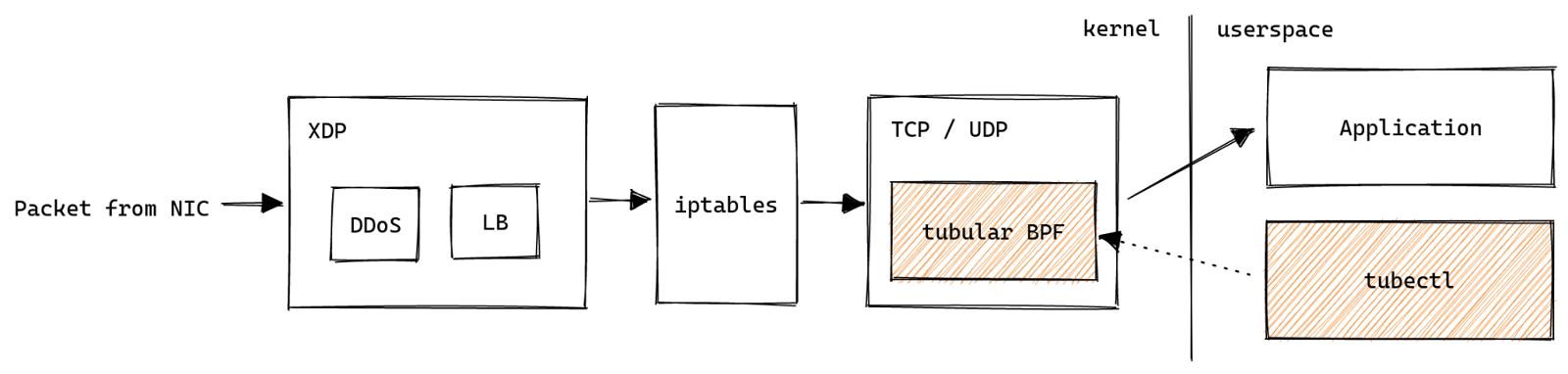
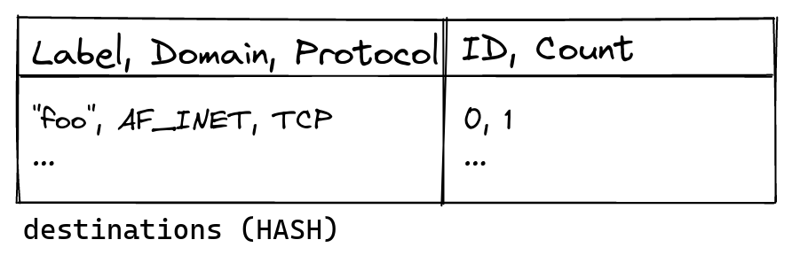
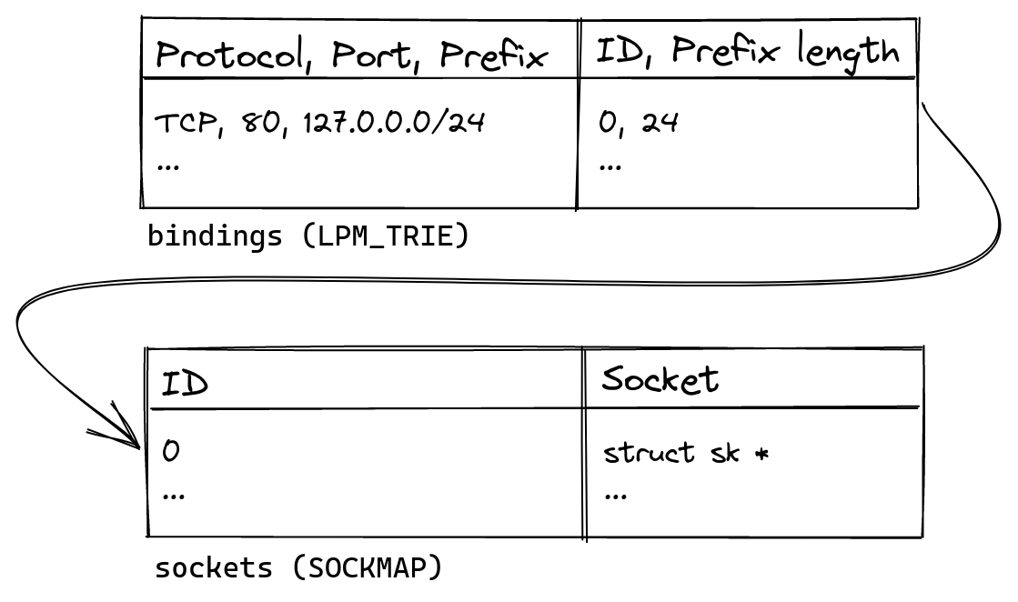
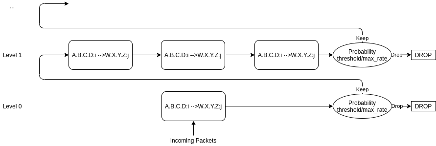
BPF trie maps (BPF_MAP_TYPE_LPM_TRIE) are heavily used for things like IP and IP+Port matching when routing network packets, ensuring your request passes through the right services before returning a result. The performance of this data structure is critical for serving our customers, but the speed of the current implementation leaves a lot to be desired. We’ve run into several bottlenecks when storing millions of entries in BPF LPM trie maps, such as entry lookup times taking hundreds of milliseconds to complete and freeing maps locking up a CPU for over 10 seconds. For instance, BPF maps are used when evaluating Cloudflare’s Magic Firewall rules and these bottlenecks have even led to traffic packet loss for some customers.

This post gives a refresher of how tries and prefix matching work, benchmark results, and a list of the shortcomings of the current BPF LPM trie implementation.

A brief recap of tries

If it’s been a while since you last looked at the trie data structure (or if you’ve never seen it before), a trie is a tree data structure (similar to a binary tree) that allows you to store and search for data for a given key and where each node stores some number of key bits.

Searches are performed by traversing a path, which essentially reconstructs the key from the traversal path, meaning nodes do not need to store their full key. This differs from a traditional binary search tree (BST) where the primary invariant is that the left child node has a key that is less than the current node and the right child has a key that is greater. BSTs require that each node store the full key so that a comparison can be made at each search step.

Here’s an example that shows how a BST might store values for the keys:

  • ABC

  • ABCD

  • ABCDEFGH

  • DEF


In comparison, a trie for storing the same set of keys might look like this.


This way of splitting out bits is really memory-efficient when you have redundancy in your data, e.g. prefixes are common in your keys, because that shared data only requires a single set of nodes. It’s for this reason that tries are often used to efficiently store strings, e.g. dictionaries of words – storing the strings “ABC” and “ABCD” doesn’t require 3 bytes + 4 bytes (assuming ASCII), it only requires 3 bytes + 1 byte because “ABC” is shared by both (the exact number of bits required in the trie is implementation dependent).

Tries also allow more efficient searching. For instance, if you wanted to know whether the key “CAR” existed in the BST you are required to go to the right child of the root (the node with key “DEF”) and check its left child because this is where it would live if it existed. A trie is more efficient because it searches in prefix order. In this particular example, a trie knows at the root whether that key is in the trie or not.

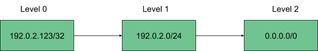
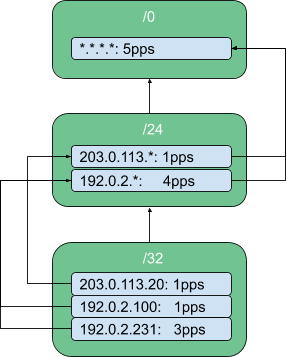
This design makes tries perfectly suited for performing longest prefix matches and for working with IP routing using CIDR. CIDR was introduced to make more efficient use of the IP address space (no longer requiring that classes fall into 4 buckets of 8 bits) but comes with added complexity because now the network portion of an IP address can fall anywhere. Handling the CIDR scheme in IP routing tables requires matching on the longest (most specific) prefix in the table rather than performing a search for an exact match.

If searching a trie does a single-bit comparison at each node, that’s a binary trie. If searching compares more bits we call that a multibit trie. You can store anything you like in a trie, including IP and subnet addresses – it’s all just ones and zeroes.

Nodes in multibit tries use more memory than in binary tries, but since computers operate on multibit words anyhow, it’s more efficient from a microarchitecture perspective to use multibit tries because you can traverse through the bits faster, reducing the number of comparisons you need to make to search for your data. It’s a classic space vs time tradeoff.

There are other optimisations we can use with tries. The distribution of data that you store in a trie might not be uniform and there could be sparsely populated areas. For example, if you store the strings “A” and “BCDEFGHI” in a multibit trie, how many nodes do you expect to use? If you’re using ASCII, you could construct the binary trie with a root node and branch left for “A” or right for “B”. With 8-bit nodes, you’d need another 7 nodes to store “C”, “D”, “E”, “F”, “G”, “H”, “I”.


Since there are no other strings in the trie, that’s pretty suboptimal. Once you hit the first level after matching on “B” you know there’s only one string in the trie with that prefix, and you can avoid creating all the other nodes by using path compression. Path compression replaces nodes “C”, “D”, “E” etc. with a single one such as “I”.


If you traverse the tree and hit “I”, you still need to compare the search key with the bits you skipped (“CDEFGH”) to make sure your search key matches the string. Exactly how and where you store the skipped bits is implementation dependent – BPF LPM tries simply store the entire key in the leaf node. As your data becomes denser, path compression is less effective.

What if your data distribution is dense and, say, all the first 3 levels in a trie are fully populated? In that case you can use level compression and replace all the nodes in those levels with a single node that has 2**3 children. This is how Level-Compressed Tries work which are used for IP route lookup in the Linux kernel (see net/ipv4/fib_trie.c).

There are other optimisations too, but this brief detour is sufficient for this post because the BPF LPM trie implementation in the kernel doesn’t fully use the three we just discussed.

How fast are BPF LPM trie maps?

Here are some numbers from running BPF selftests benchmark on AMD EPYC 9684X 96-Core machines. Here the trie has 10K entries, a 32-bit prefix length, and an entry for every key in the range [0, 10K).

Operation

Throughput

Stddev

Latency

lookup

7.423M ops/s

0.023M ops/s

134.710 ns/op

update

2.643M ops/s

0.015M ops/s

378.310 ns/op

delete

0.712M ops/s

0.008M ops/s

1405.152 ns/op

free

0.573K ops/s

0.574K ops/s

1.743 ms/op

The time to free a BPF LPM trie with 10K entries is noticeably large. We recently ran into an issue where this took so long that it caused soft lockup messages to spew in production.

This benchmark gives some idea of worst case behaviour. Since the keys are so densely populated, path compression is completely ineffective. In the next section, we explore the lookup operation to understand the bottlenecks involved.

Why are BPF LPM tries slow?

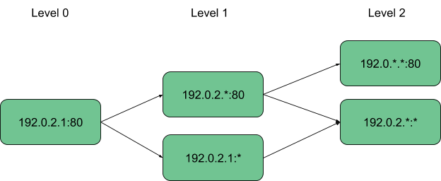
The LPM trie implementation in kernel/bpf/lpm_trie.c has a couple of the optimisations we discussed in the introduction. It is capable of multibit comparisons at leaf nodes, but since there are only two child pointers in each internal node, if your tree is densely populated with a lot of data that only differs by one bit, these multibit comparisons degrade into single bit comparisons.

Here’s an example. Suppose you store the numbers 0, 1, and 3 in a BPF LPM trie. You might hope that since these values fit in a single 32 or 64-bit machine word, you could use a single comparison to decide which next node to visit in the trie. But that’s only possible if your trie implementation has 3 child pointers in the current node (which, to be fair, most trie implementations do). In other words, you want to make a 3-way branching decision but since BPF LPM tries only have two children, you’re limited to a 2-way branch.

A diagram for this 2-child trie is given below.


The leaf nodes are shown in green with the key, as a binary string, in the center. Even though a single 8-bit comparison is more than capable of figuring out which node has that key, the BPF LPM trie implementation resorts to inserting intermediate nodes (blue) to inject 2-way branching decisions into your path traversal because its parent (the orange root node in this case) only has 2 children. Once you reach a leaf node, BPF LPM tries can perform a multibit comparison to check the key. If a node supported pointers to more children, the above trie could instead look like this, allowing a 3-way branch and reducing the lookup time.


This 2-child design impacts the height of the trie. In the worst case, a completely full trie essentially becomes a binary search tree with height log2(nr_entries) and the height of the trie impacts how many comparisons are required to search for a key.

The above trie also shows how BPF LPM tries implement a form of path compression – you only need to insert an intermediate node where you have two nodes whose keys differ by a single bit. If instead of 3, you insert a key of 15 (0b1111), this won’t change the layout of the trie; you still only need a single node at the right child of the root.


And finally, BPF LPM tries do not implement level compression. Again, this stems from the fact that nodes in the trie can only have 2 children. IP route tables tend to have many prefixes in common and you typically see densely packed tries at the upper levels which makes level compression very effective for tries containing IP routes.

Here’s a graph showing how the lookup throughput for LPM tries (measured in million ops/sec) degrades as the number of entries increases, from 1 entry up to 100K entries.


Once you reach 1 million entries, throughput is around 1.5 million ops/sec, and continues to fall as the number of entries increases.


Why is this? Initially, this is because of the L1 dcache miss rate. All of those nodes that need to be traversed in the trie are potential cache miss opportunities.


As you can see from the graph, L1 dcache miss rate remains relatively steady and yet the throughput continues to decline. At around 80K entries, dTLB miss rate becomes the bottleneck.


Because BPF LPM tries to dynamically allocate individual nodes from a freelist of kernel memory, these nodes can live at arbitrary addresses. Which means traversing a path through a trie almost certainly will incur cache misses and potentially dTLB misses. This gets worse as the number of entries, and height of the trie, increases.


Where do we go from here?

By understanding the current limitations of the BPF LPM trie, we can now work towards building a more performant and efficient solution for the future of the Internet.

We’ve already contributed these benchmarks to the upstream Linux kernel — but that’s only the start. We have plans to improve the performance of BPM LPM tries, particularly the lookup function which is heavily used for our workloads. This post covered a number of optimisations that are already used by the net/ipv4/fib_trie.c code, so a natural first step is to refactor that code so that a common Level Compressed trie implementation can be used. Expect future blog posts to explore this work in depth.

If you’re interested in looking at more performance numbers, Jesper Brouer has recorded some here: https://github.com/xdp-project/xdp-project/blob/main/areas/bench/bench02_lpm-trie-lookup.org.

If the Linux kernel, performance, or optimising data structures excites you, our engineering teams are hiring.

How Netflix Accurately Attributes eBPF Flow Logs

Post Syndicated from Netflix Technology Blog original https://netflixtechblog.com/how-netflix-accurately-attributes-ebpf-flow-logs-afe6d644a3bc

By Cheng Xie, Bryan Shultz, and Christine Xu

In a previous blog post, we described how Netflix uses eBPF to capture TCP flow logs at scale for enhanced network insights. In this post, we delve deeper into how Netflix solved a core problem: accurately attributing flow IP addresses to workload identities.

A Brief Recap

FlowExporter is a sidecar that runs alongside all Netflix workloads. It uses eBPF and TCP tracepoints to monitor TCP socket state changes. When a TCP socket closes, FlowExporter generates a flow log record that includes the IP addresses, ports, timestamps, and additional socket statistics. On average, 5 million records are produced per second.

In cloud environments, IP addresses are reassigned to different workloads as workload instances are created and terminated, so IP addresses alone cannot provide insights on which workloads are communicating. To make the flow logs useful, each IP address must be attributed to its corresponding workload identity. FlowCollector, a backend service, collects flow logs from FlowExporter instances across the fleet, attributes the IP addresses, and sends these attributed flows to Netflix’s Data Mesh for subsequent stream and batch processing.

The eBPF flow logs provide a comprehensive view of service topology and network health across Netflix’s extensive microservices fleet, regardless of the programming language, RPC mechanism, or application-layer protocol used by individual workloads.

The Problem with Misattribution

Accurately attributing flow IP addresses to workload identities has been a significant challenge since our eBPF flow logs were introduced.

As noted in our previous blog post, our initial attribution approach relied on Sonar, an internal IP address tracking service that emits an event whenever an IP address in Netflix’s AWS VPCs is assigned or unassigned to a workload. FlowCollector consumes a stream of IP address change events from Sonar and uses this information to attribute flow IP addresses in real-time.

The fundamental drawback of this method is that it can lead to misattribution. Delays and failures are inevitable in distributed systems, which may delay IP address change events from reaching FlowCollector. For instance, an IP address may initially be assigned to workload X but later reassigned to workload Y. However, if the change event for this reassignment is delayed, FlowCollector will continue to assume that the IP address belongs to workload X, resulting in misattributed flows. Additionally, event timestamps may be inaccurate depending on how they are captured.

Misattribution rendered the flow data unreliable for decision-making. Users often depend on flow logs to validate workload dependencies, but misattribution creates confusion. Without expert knowledge of expected dependencies, users would struggle to identify or confirm misattribution. Moreover, misattribution occurred frequently for critical services with a large footprint due to frequent IP address changes. Overall, misattribution makes fleet-wide dependency analysis impractical.

As a workaround, we made FlowCollector hold received flows for 15 minutes before attribution, allowing time for delayed IP address change events. While this approach reduced misattribution, it did not eliminate it. Moreover, the waiting period made the data less fresh, reducing its utility for real-time analysis.

Fully eliminating misattribution is crucial because it only takes a single misattributed flow to produce an incorrect workload dependency. Solving this problem required a complete rethinking of our approach. Over the past year, Netflix developed a new attribution method that has finally eliminated misattribution, as detailed in the rest of this post.

Attributing Local IP Addresses

Each socket has two IP addresses: a local IP address and a remote IP address. Previously, we used the same method to attribute both. However, attributing the local IP address should be a simpler task since the local IP address belongs to the instance where FlowExporter captures the socket. Therefore, FlowExporter should determine the local workload identity from its environment and attribute the local IP address before sending the flow to FlowCollector.

This is straightforward for workloads running directly on EC2 instances, as Netflix’s Metatron provisions workload identity certificates to each EC2 instance at boot time. FlowExporter can simply read these certificates from the local disk to determine the local workload identity.

Attributing local IP addresses for container workloads running on Netflix’s container platform, Titus, is more challenging. FlowExporter runs at the container host level, where each host manages multiple container workloads with different identities. When FlowExporter’s eBPF programs receive a socket event from TCP tracepoints in the kernel, the socket may have been created by one of the container workloads or by the host itself. Therefore, FlowExporter must determine which workload to attribute the socket’s local IP address to. To solve this problem, we leveraged IPMan, Netflix’s container IP address assignment service. IPManAgent, a daemon running on every container host, is responsible for assigning and unassigning IP addresses. As container workloads are launched, IPManAgent writes an IP-address-to-workload-ID mapping to an eBPF map, which FlowExporter’s eBPF programs can then use to look up the workload ID associated with a socket local IP address.

Another challenge was to accommodate Netflix’s IPv6 to IPv4 translation mechanism on Titus. To facilitate IPv6 migration, Netflix developed a mechanism that enables IPv6-only containers to communicate with IPv4 destinations without incurring NAT64 overhead. This mechanism intercepts connect syscalls and replaces the underlying socket with one that uses a shared IPv4 address assigned to the container host. This confuses FlowExporter because the kernel reports the same local IPv4 address for sockets created by different container workloads. To disambiguate, local port information is additionally required. We modified Titus to write a mapping of (local IPv4 address, local port) to the workload ID into an eBPF map whenever a connect syscall is intercepted. FlowExporter’s eBPF programs then use this map to correctly attribute sockets created by the translation mechanism.

With these problems solved, we can now accurately attribute the local IP address of every flow.

Attributing Remote IP Addresses

Once the local IP address attribution problem is solved, accurately attributing remote IP addresses becomes feasible. Now, each flow reported by FlowExporter includes the local IP address, the local workload identity, and connection start/end timestamps. As FlowCollector receives these flows, it can learn the time ranges during which each workload owns a given IP address. For instance, if FlowCollector sees a flow with local IP address 10.0.0.1 associated with workload X that starts at t1 and ends at t2, it can deduce that 10.0.0.1 belonged to workload X from t1 to t2. Since Netflix uses Amazon Time Sync across its fleet, the timestamps (captured by FlowExporter) are reliable.

The FlowCollector service cluster consists of many nodes. Every node must be capable of attributing arbitrary remote IP addresses and, therefore, requires knowledge of all workload IP addresses and their recent ownership records. To represent this knowledge, each node maintains an in-memory hashmap that maps an IP address to a list of time ranges, as illustrated by the following Go structs:

type IPAddressTracker struct {
ipToTimeRanges map[netip.Addr]timeRanges
}

type timeRanges []timeRange

type timeRange struct {
workloadID string
start time.Time
end time.Time
}

To populate the hashmap, FlowCollector extracts the local IP address, local workload identity, start time, and end time from each received flow and creates/extends the corresponding time ranges in the map. The time ranges for each IP address are sorted in ascending order, and they are non-overlapping since an IP address cannot belong to two different workloads simultaneously.

Since each flow is only sent to one FlowCollector node, each node must share the time ranges it learned from received flows with other nodes. We implemented a broadcasting mechanism using Kafka, where each node publishes learned time ranges to all other nodes. Although more efficient broadcasting implementations exist, the Kafka-based approach is simple and has worked well for us.

Now, FlowCollector can attribute remote IP addresses by looking them up in the populated map, which returns a list of time ranges. It then uses the flow’s start timestamp to determine the corresponding time range and associated workload identity. If the start time does not fall within any time range, FlowCollector will retry after a delay, eventually giving up if the retry fails. Such failures may occur when flows are lost or broadcast messages are delayed. For our use cases, it is acceptable to leave a small percentage of flows unattributed, but any misattribution is unacceptable.

This new method achieves accurate attribution thanks to the continuous heartbeats, each associated with a reliable time range of IP address ownership. It handles transient issues gracefully — a few delayed or lost heartbeats do not lead to misattribution. In contrast, the previous method relied solely on discrete IP address assignment and unassignment events. Lacking heartbeats, it had to presume an IP address remained assigned until notified otherwise (which can be hours or days later), making it vulnerable to misattribution when the notifications were delayed.

One detail is that when FlowCollector receives a flow, it cannot attribute its remote IP address right away because it requires the latest observed time ranges for the remote IP address. Since FlowExporter reports flows in batches every minute, FlowCollector must wait until it receives the flow batch from the remote workload FlowExporter for the last minute, which may not have arrived yet. To address this, FlowCollector temporarily stores received flows on disk for one minute before attributing their remote IP addresses. This introduces a 1-minute delay, but it is much shorter than the 15-minute delay with the previous approach.

In addition to producing accurate attribution, the new method is also cost-effective thanks to its simplicity and in-memory lookups. Because the in-memory state can be quickly rebuilt when a FlowCollector node starts up, no persistent storage is required. With 30 c7i.2xlarge instances, we can process 5 million flows per second across the entire Netflix fleet.

Attributing Cross-Regional IP Addresses

For simplicity, we have so far glossed over one topic: regionalization. Netflix’s cloud microservices operate across multiple AWS regions. To optimize flow reporting and minimize cross-regional traffic, a FlowCollector cluster runs in each major region, and FlowExporter agents send flows to their corresponding regional FlowCollector. When FlowCollector receives a flow, its local IP address is guaranteed to be within the region.

To minimize cross-region traffic, the broadcasting mechanism is limited to FlowCollector nodes within the same region. Consequently, the IP address time ranges map contains only IP addresses from that region. However, cross-regional flows have a remote IP address in a different region. To attribute these flows, the receiving FlowCollector node forwards them to nodes in the corresponding region. FlowCollector determines the region for a remote IP address by looking up a trie built from all Netflix VPC CIDRs. This approach is more efficient than broadcasting IP address time range updates across all regions, as only 1% of Netflix flows are cross-regional.

Attributing Non-Workload IP Addresses

So far, FlowCollector can accurately attribute IP addresses belonging to Netflix’s cloud workloads. However, not all flow IP addresses fall into this category. For instance, a significant portion of flows goes through AWS ELBs. For these flows, their remote IP addresses are associated with the ELBs, where we cannot run FlowExporter. Consequently, FlowCollector cannot determine their identities by simply observing the received flows. To attribute these remote IP addresses, we continue to use IP address change events from Sonar, which crawls AWS resources to detect changes in IP address assignments. Although this data stream may contain inaccurate timestamps and be delayed, misattribution is not a main concern since ELB IP address reassignment occurs very infrequently.

Verifying Correctness

Verifying that the new method has eliminated misattribution is challenging due to the lack of a definitive source of truth for workload dependencies to validate flow logs against; the flow logs themselves are intended to serve as this source of truth, after all. To build confidence, we analyzed the flow logs of a large service with well-understood dependencies. A large footprint is necessary, as misattribution is more prevalent in services with numerous instances, and there must be a reliable method to determine the dependencies for this service without relying on flow logs.

Netflix’s cloud gateway, Zuul, served this purpose perfectly due to its extensive footprint (handling all cloud ingress traffic), its large number of downstream dependencies, and our ability to derive its dependencies from its routing configurations as the source of truth for comparison with flow logs. We found no misattribution for flows through Zuul over a two-week window. This provided strong confidence that the new attribution method has eliminated misattribution. In the previous approach, approximately 40% of Zuul’s dependencies reported by the flow logs were misattributed.

Conclusion

With misattribution solved, eBPF flow logs now deliver dependable, fleet-wide insights into Netflix’s service topology and network health. This advancement unlocks numerous exciting opportunities in areas such as service dependency auditing, security analysis, and incident triage, while helping Netflix engineers develop a better understanding of our ever-evolving distributed systems.

Acknowledgments

We would like to thank Martin Dubcovsky, Joanne Koong, Taras Roshko, Nabil Schear, Jacob Meyers, Parsha Pourkhomami, Hechao Li, Donavan Fritz, Rob Gulewich, Amanda Li, John Salem, Hariharan Ananthakrishnan, Keerti Lakshminarayan, and other stunning colleagues for their feedback, inspiration, and contributions to the success of this effort.


How Netflix Accurately Attributes eBPF Flow Logs was originally published in Netflix TechBlog on Medium, where people are continuing the conversation by highlighting and responding to this story.

Noisy Neighbor Detection with eBPF

Post Syndicated from Netflix Technology Blog original https://netflixtechblog.com/noisy-neighbor-detection-with-ebpf-64b1f4b3bbdd

By Jose Fernandez, Sebastien Dabdoub, Jason Koch, Artem Tkachuk

The Compute and Performance Engineering teams at Netflix regularly investigate performance issues in our multi-tenant environment. The first step is determining whether the problem originates from the application or the underlying infrastructure. One issue that often complicates this process is the "noisy neighbor" problem. On Titus, our multi-tenant compute platform, a "noisy neighbor" refers to a container or system service that heavily utilizes the server's resources, causing performance degradation in adjacent containers. We usually focus on CPU utilization because it is our workload's most frequent source of noisy neighbor issues.

Detecting the effects of noisy neighbors is complex. Traditional performance analysis tools such as perf can introduce significant overhead, risking further performance degradation. Additionally, these tools are typically deployed after the fact, which is too late for effective investigation. Another challenge is that debugging noisy neighbor issues requires significant low-level expertise and specialized tooling. In this blog post, we'll reveal how we leveraged eBPF to achieve continuous, low-overhead instrumentation of the Linux scheduler, enabling effective self-serve monitoring of noisy neighbor issues. Learn how Linux kernel instrumentation can improve your infrastructure observability with deeper insights and enhanced monitoring.

Continuous Instrumentation of the Linux Scheduler

To ensure the reliability of our workloads that depend on low latency responses, we instrumented the run queue latency for each container, which measures the time processes spend in the scheduling queue before being dispatched to the CPU. Extended waiting in this queue can be a telltale of performance issues, especially when containers are not utilizing their total CPU allocation. Continuous instrumentation is critical to catching such matters as they emerge, and eBPF, with its hooks into the Linux scheduler with minimal overhead, enabled us to monitor run queue latency efficiently.

To emit a run queue latency metric, we leveraged three eBPF hooks: sched_wakeup, sched_wakeup_new, and sched_switch.

The sched_wakeup and sched_wakeup_new hooks are invoked when a process changes state from 'sleeping' to 'runnable.' They let us identify when a process is ready to run and is waiting for CPU time. During this event, we generate a timestamp and store it in an eBPF hash map using the process ID as the key.

struct {
__uint(type, BPF_MAP_TYPE_HASH);
__uint(max_entries, MAX_TASK_ENTRIES);
__uint(key_size, sizeof(u32));
__uint(value_size, sizeof(u64));
} runq_lat SEC(".maps");

SEC("tp_btf/sched_wakeup")
int tp_sched_wakeup(u64 *ctx)
{
struct task_struct *task = (void *)ctx[0];
u32 pid = task->pid;
u64 ts = bpf_ktime_get_ns();

bpf_map_update_elem(&runq_lat, &pid, &ts, BPF_NOEXIST);
return 0;
}

Conversely, the sched_switch hook is triggered when the CPU switches between processes. This hook provides pointers to the process currently utilizing the CPU and the process about to take over. We use the upcoming task's process ID (PID) to fetch the timestamp from the eBPF map. This timestamp represents when the process entered the queue, which we had previously stored. We then calculate the run queue latency by simply subtracting the timestamps.

SEC("tp_btf/sched_switch")
int tp_sched_switch(u64 *ctx)
{
struct task_struct *prev = (struct task_struct *)ctx[1];
struct task_struct *next = (struct task_struct *)ctx[2];
u32 prev_pid = prev->pid;
u32 next_pid = next->pid;

// fetch timestamp of when the next task was enqueued
u64 *tsp = bpf_map_lookup_elem(&runq_lat, &next_pid);
if (tsp == NULL) {
return 0; // missed enqueue
}

// calculate runq latency before deleting the stored timestamp
u64 now = bpf_ktime_get_ns();
u64 runq_lat = now - *tsp;

// delete pid from enqueued map
bpf_map_delete_elem(&runq_lat, &next_pid);
....

One of the advantages of eBPF is its ability to provide pointers to the actual kernel data structures representing processes or threads, also known as tasks in kernel terminology. This feature enables access to a wealth of information stored about a process. We required the process's cgroup ID to associate it with a container for our specific use case. However, the cgroup information in the struct is safeguarded by an RCU (Read Copy Update) lock.

To safely access this RCU-protected information, we can leverage kfuncs in eBPF. kfuncs are kernel functions that can be called from eBPF programs. There are kfuncs available to lock and unlock RCU read-side critical sections. These functions ensure that our eBPF program remains safe and efficient while retrieving the cgroup ID from the task struct.

void bpf_rcu_read_lock(void) __ksym;
void bpf_rcu_read_unlock(void) __ksym;

u64 get_task_cgroup_id(struct task_struct *task)
{
struct css_set *cgroups;
u64 cgroup_id;
bpf_rcu_read_lock();
cgroups = task->cgroups;
cgroup_id = cgroups->dfl_cgrp->kn->id;
bpf_rcu_read_unlock();
return cgroup_id;
}

Having the data ready, we must package it and send it to userspace. For this purpose, we chose the eBPF ring buffer. It is efficient, high-performing, and user-friendly. It can handle variable-length data records and allows data reading without necessitating extra memory copying or syscalls. However, the sheer amount of data points was causing the userspace program to use too much CPU, so we implemented a rate limiter in eBPF to sample the data effectively.

struct {
__uint(type, BPF_MAP_TYPE_RINGBUF);
__uint(max_entries, 256 * 1024);
} events SEC(".maps");

struct {
__uint(type, BPF_MAP_TYPE_PERCPU_HASH);
__uint(max_entries, MAX_TASK_ENTRIES);
__uint(key_size, sizeof(u64));
__uint(value_size, sizeof(u64));
} cgroup_id_to_last_event_ts SEC(".maps");

struct runq_event {
u64 prev_cgroup_id;
u64 cgroup_id;
u64 runq_lat;
u64 ts;
};

SEC("tp_btf/sched_switch")
int tp_sched_switch(u64 *ctx)
{
// ....
// The previous code
// ....

u64 prev_cgroup_id = get_task_cgroup_id(prev);
u64 cgroup_id = get_task_cgroup_id(next);

// per-cgroup-id-per-CPU rate-limiting
// to balance observability with performance overhead
u64 *last_ts =
bpf_map_lookup_elem(&cgroup_id_to_last_event_ts, &cgroup_id);
u64 last_ts_val = last_ts == NULL ? 0 : *last_ts;

// check the rate limit for the cgroup_id in consideration
// before doing more work
if (now - last_ts_val < RATE_LIMIT_NS) {
// Rate limit exceeded, drop the event
return 0;
}

struct runq_event *event;
event = bpf_ringbuf_reserve(&events, sizeof(*event), 0);

if (event) {
event->prev_cgroup_id = prev_cgroup_id;
event->cgroup_id = cgroup_id;
event->runq_lat = runq_lat;
event->ts = now;
bpf_ringbuf_submit(event, 0);
// Update the last event timestamp for the current cgroup_id
bpf_map_update_elem(&cgroup_id_to_last_event_ts, &cgroup_id,
&now, BPF_ANY);

}

return 0;
}

Our userspace application, developed in Go, processes events from the ring buffer to emit metrics to our metrics backend, Atlas. Each event includes a run queue latency sample with a cgroup ID, which we associate with running containers on the host. We categorize it as a system service if no such association is found. When a cgroup ID correlates with a container, we emit a percentile timer Atlas metric (runq.latency) for that container. We also increment a counter metric (sched.switch.out) to monitor preemptions occurring for the container's processes. Access to the prev_cgroup_id of the preempted process allows us to tag the metric with the cause of the preemption, whether it's due to a process within the same container (or cgroup), a process in another container, or a system service.

It's important to highlight that both the runq.latency metric and the sched.switch.out metrics are needed to determine if a container is affected by noisy neighbors, which is the goal we aim to achieve — relying solely on the runq.latency metric can lead to misconceptions. For example, if a container is at or over its cgroup CPU limit, the scheduler will throttle it, resulting in an apparent spike in run queue latency due to delays in the queue. If we were only to consider this metric, we might incorrectly attribute the performance degradation to noisy neighbors when it's actually because the container is hitting its CPU request limits. However, simultaneous spikes in both metrics, mainly when the cause is a different container or system process, clearly indicate a noisy neighbor issue.

A Noisy Neighbor Story

Below is the runq.latency metric for a server running a single container with ample CPU overhead. The 99th percentile averages 83.4µs (microseconds), serving as our baseline. Although there are some spikes reaching 400µs, the latency remains within acceptable parameters.

container1’s 99th percentile runq.latency averages 83µs (microseconds), with spikes up to 400µs, without adjacent containers. This serves as our baseline for a container not contending for CPU on a host.

At 10:35, launching container2, which fully utilized all CPUs on the host, caused a significant 131-millisecond spike (131,000 microseconds) in container1's P99 run queue latency. This spike would be noticeable in the userspace application if it were serving HTTP traffic. If userspace app owners reported an unexplained latency spike, we could quickly identify the noisy neighbor issue through run queue latency metrics.

Launching container2 at 10:35, which maxes out all CPUs on the host, caused a 131-millisecond spike in container1’s P99 run queue latency due to increased preemptions by system processes. This indicates a noisy neighbor issue, where system services compete for CPU time with containers.

The sched.switch.out metric indicates that the spike was due to increased preemptions by system processes, highlighting a noisy neighbor issue where system services compete with containers for CPU time. Our metrics show that the noisy neighbors were actually system processes, likely triggered by container2 consuming all available CPU capacity.

Optimizing eBPF Code

We developed an open-source eBPF process monitor called bpftop to measure the overhead of eBPF code in this hot kernel path. Our estimates suggest that the instrumentation adds less than 600 nanoseconds to each sched_* hook. We conducted a performance analysis on a Java service running in a container, and the instrumentation did not introduce significant overhead. The performance variance with the run queue profiling code active versus inactive was not measurable in milliseconds.

During our research on how eBPF statistics are measured in the kernel, we identified an opportunity to improve its calculation. We submitted this patch, which was included in the Linux kernel 6.10 release.

Through trial and error and using bpftop, we identified several optimizations that helped maintain low overhead for this code:

  • We found that BPF_MAP_TYPE_HASH was the most performant for storing enqueued timestamps. Using BPF_MAP_TYPE_TASK_STORAGE resulted in nearly a twofold performance decline. BPF_MAP_TYPE_PERCPU_HASH was slightly less performant than BPF_MAP_TYPE_HASH, which was unexpected and requires further investigation.
  • The BPF_CORE_READ helper adds 20–30 nanoseconds per invocation. In the case of raw tracepoints, specifically those that are "BTF-enabled" (tp_btf/*), it is safe and more efficient to access the task struct members directly. Andrii Nakryiko recommends this approach in this blog post.
  • BPF_MAP_TYPE_LRU_HASH maps are 40–50 nanoseconds slower per operation than regular hash maps. Due to space concerns from PID churn, we initially used them for enqueued timestamps. We have since increased the map size, mitigating this risk.
  • The sched_switch, sched_wakeup, and sched_wakeup_new are all triggered for kernel tasks, which are identifiable by their PID of 0. We found monitoring these tasks unnecessary, so we implemented several early exit conditions and conditional logic to prevent executing costly operations, such as accessing BPF maps, when dealing with a kernel task. Notably, kernel tasks operate through the scheduler queue like any regular process.

Conclusion

Our findings highlight the value of low-overhead continuous instrumentation of the Linux kernel with eBPF. We have integrated these metrics into customer dashboards, enabling actionable insights and guiding multitenancy performance discussions. We can also now use these metrics to refine CPU isolation strategies to minimize the impact of noisy neighbors. Additionally, thanks to these metrics, we've gained deeper insights into the Linux scheduler.

This project has also deepened our understanding of eBPF technology and underscored the importance of tools like bpftop for optimizing eBPF code. As eBPF adoption increases, we foresee more infrastructure observability and business logic shifting to it. One promising project in this space is sched_ext, potentially revolutionizing how scheduling decisions are made and tailored to specific workload needs.


Noisy Neighbor Detection with eBPF was originally published in Netflix TechBlog on Medium, where people are continuing the conversation by highlighting and responding to this story.

Announcing bpftop: Streamlining eBPF performance optimization

Post Syndicated from Netflix Technology Blog original https://netflixtechblog.com/announcing-bpftop-streamlining-ebpf-performance-optimization-6a727c1ae2e5

By Jose Fernandez

Today, we are thrilled to announce the release of bpftop, a command-line tool designed to streamline the performance optimization and monitoring of eBPF applications. As Netflix increasingly adopts eBPF [1, 2], applying the same rigor to these applications as we do to other managed services is imperative. Striking a balance between eBPF’s benefits and system load is crucial, ensuring it enhances rather than hinders our operational efficiency. This tool enables Netflix to embrace eBPF’s potential.

Introducing bpftop

bpftop provides a dynamic real-time view of running eBPF programs. It displays the average execution runtime, events per second, and estimated total CPU % for each program. This tool minimizes overhead by enabling performance statistics only while it is active.

bpftop simplifies the performance optimization process for eBPF programs by enabling an efficient cycle of benchmarking, code refinement, and immediate feedback. Without bpftop, optimization efforts would require manual calculations, adding unnecessary complexity to the process. With bpftop, users can quickly establish a baseline, implement improvements, and verify enhancements, streamlining the process.

A standout feature of this tool is its ability to display the statistics in time series graphs. This approach can uncover patterns and trends that could be missed otherwise.

How it works

bpftop uses the BPF_ENABLE_STATS syscall command to enable global eBPF runtime statistics gathering, which is disabled by default to reduce performance overhead. It collects these statistics every second, calculating the average runtime, events per second, and estimated CPU utilization for each eBPF program within that sample period. This information is displayed in a top-like tabular format or a time series graph over a 10s moving window. Once bpftop terminates, it turns off the statistics-gathering function. The tool is written in Rust, leveraging the libbpf-rs and ratatui crates.

Getting started

Visit the project’s GitHub page to learn more about using the tool. We’ve open-sourced bpftop under the Apache 2 license and look forward to contributions from the community.


Announcing bpftop: Streamlining eBPF performance optimization was originally published in Netflix TechBlog on Medium, where people are continuing the conversation by highlighting and responding to this story.

A July 4 technical reading list

Post Syndicated from John Graham-Cumming original https://blog.cloudflare.com/july-4-2022-reading-list/

A July 4 technical reading list

A July 4 technical reading list

Here’s a short list of recent technical blog posts to give you something to read today.

Internet Explorer, we hardly knew ye

Microsoft has announced the end-of-life for the venerable Internet Explorer browser. Here we take a look at the demise of IE and the rise of the Edge browser. And we investigate how many bots on the Internet continue to impersonate Internet Explorer versions that have long since been replaced.

Live-patching security vulnerabilities inside the Linux kernel with eBPF Linux Security Module

Looking for something with a lot of technical detail? Look no further than this blog about live-patching the Linux kernel using eBPF. Code, Makefiles and more within!

Hertzbleed explained

Feeling mathematical? Or just need a dose of CPU-level antics? Look no further than this deep explainer about how CPU frequency scaling leads to a nasty side channel affecting cryptographic algorithms.

Early Hints update: How Cloudflare, Google, and Shopify are working together to build a faster Internet for everyone

The HTTP standard for Early Hints shows a lot of promise. How much? In this blog post, we dig into data about Early Hints in the real world and show how much faster the web is with it.

Private Access Tokens: eliminating CAPTCHAs on iPhones and Macs with open standards

Dislike CAPTCHAs? Yes, us too. As part of our program to eliminate captures there’s a new standard: Private Access Tokens. This blog shows how they work and how they can be used to prove you’re human without saying who you are.

Optimizing TCP for high WAN throughput while preserving low latency

Network nerd? Yeah, me too. Here’s a very in depth look at how we tune TCP parameters for low latency and high throughput.

Production ready eBPF, or how we fixed the BSD socket API

Post Syndicated from Lorenz Bauer original https://blog.cloudflare.com/tubular-fixing-the-socket-api-with-ebpf/

Production ready eBPF, or how we fixed the BSD socket API

Production ready eBPF, or how we fixed the BSD socket API

As we develop new products, we often push our operating system – Linux – beyond what is commonly possible. A common theme has been relying on eBPF to build technology that would otherwise have required modifying the kernel. For example, we’ve built DDoS mitigation and a load balancer and use it to monitor our fleet of servers.

This software usually consists of a small-ish eBPF program written in C, executed in the context of the kernel, and a larger user space component that loads the eBPF into the kernel and manages its lifecycle. We’ve found that the ratio of eBPF code to userspace code differs by an order of magnitude or more. We want to shed some light on the issues that a developer has to tackle when dealing with eBPF and present our solutions for building rock-solid production ready applications which contain eBPF.

For this purpose we are open sourcing the production tooling we’ve built for the sk_lookup hook we contributed to the Linux kernel, called tubular. It exists because we’ve outgrown the BSD sockets API. To deliver some products we need features that are just not possible using the standard API.

  • Our services are available on millions of IPs.
  • Multiple services using the same port on different addresses have to coexist, e.g. 1.1.1.1 resolver and our authoritative DNS.
  • Our Spectrum product needs to listen on all 2^16 ports.

The source code for tubular is at https://github.com/cloudflare/tubular, and it allows you to do all the things mentioned above. Maybe the most interesting feature is that you can change the addresses of a service on the fly:

How tubular works

tubular sits at a critical point in the Cloudflare stack, since it has to inspect every connection terminated by a server and decide which application should receive it.

Production ready eBPF, or how we fixed the BSD socket API

Failure to do so will drop or misdirect connections hundreds of times per second. So it has to be incredibly robust during day to day operations. We had the following goals for tubular:

  • Releases must be unattended and happen online
    tubular runs on thousands of machines, so we can’t babysit the process or take servers out of production.
  • Releases must fail safely
    A failure in the process must leave the previous version of tubular running, otherwise we may drop connections.
  • Reduce the impact of (userspace) crashes
    When the inevitable bug comes along we want to minimise the blast radius.

In the past we had built a proof-of-concept control plane for sk_lookup called inet-tool, which proved that we could get away without a persistent service managing the eBPF. Similarly, tubular has tubectl: short-lived invocations make the necessary changes and persisting state is handled by the kernel in the form of eBPF maps. Following this design gave us crash resiliency by default, but left us with the task of mapping the user interface we wanted to the tools available in the eBPF ecosystem.

The tubular user interface

tubular consists of a BPF program that attaches to the sk_lookup hook in the kernel and userspace Go code which manages the BPF program. The tubectl command wraps both in a way that is easy to distribute.

tubectl manages two kinds of objects: bindings and sockets. A binding encodes a rule against which an incoming packet is matched. A socket is a reference to a TCP or UDP socket that can accept new connections or packets.

Bindings and sockets are “glued” together via arbitrary strings called labels. Conceptually, a binding assigns a label to some traffic. The label is then used to find the correct socket.

Production ready eBPF, or how we fixed the BSD socket API

Adding bindings

To create a binding that steers port 80 (aka HTTP) traffic destined for 127.0.0.1 to the label “foo” we use tubectl bind:

$ sudo tubectl bind "foo" tcp 127.0.0.1 80

Due to the power of sk_lookup we can have much more powerful constructs than the BSD API. For example, we can redirect connections to all IPs in 127.0.0.0/24 to a single socket:

$ sudo tubectl bind "bar" tcp 127.0.0.0/24 80

A side effect of this power is that it’s possible to create bindings that “overlap”:

1: tcp 127.0.0.1/32 80 -> "foo"
2: tcp 127.0.0.0/24 80 -> "bar"

The first binding says that HTTP traffic to localhost should go to “foo”, while the second asserts that HTTP traffic in the localhost subnet should go to “bar”. This creates a contradiction, which binding should we choose? tubular resolves this by defining precedence rules for bindings:

  1. A prefix with a longer mask is more specific, e.g. 127.0.0.1/32 wins over 127.0.0.0/24.
  2. A port is more specific than the port wildcard, e.g. port 80 wins over “all ports” (0).

Applying this to our example, HTTP traffic to all IPs in 127.0.0.0/24 will be directed to foo, except for 127.0.0.1 which goes to bar.

Getting ahold of sockets

sk_lookup needs a reference to a TCP or a UDP socket to redirect traffic to it. However, a socket is usually accessible only by the process which created it with the socket syscall. For example, an HTTP server creates a TCP listening socket bound to port 80. How can we gain access to the listening socket?

A fairly well known solution is to make processes cooperate by passing socket file descriptors via SCM_RIGHTS messages to a tubular daemon. That daemon can then take the necessary steps to hook up the socket with sk_lookup. This approach has several drawbacks:

  1. Requires modifying processes to send SCM_RIGHTS
  2. Requires a tubular daemon, which may crash

There is another way of getting at sockets by using systemd, provided socket activation is used. It works by creating an additional service unit with the correct Sockets setting. In other words: we can leverage systemd oneshot action executed on creation of a systemd socket service, registering the socket into tubular. For example:

[Unit]
Requisite=foo.socket

[Service]
Type=oneshot
Sockets=foo.socket
ExecStart=tubectl register "foo"

Since we can rely on systemd to execute tubectl at the correct times we don’t need a daemon of any kind. However, the reality is that a lot of popular software doesn’t use systemd socket activation. Dealing with systemd sockets is complicated and doesn’t invite experimentation. Which brings us to the final trick: pidfd_getfd:

The pidfd_getfd() system call allocates a new file descriptor in the calling process. This new file descriptor is a duplicate of an existing file descriptor, targetfd, in the process referred to by the PID file descriptor pidfd.

We can use it to iterate all file descriptors of a foreign process, and pick the socket we are interested in. To return to our example, we can use the following command to find the TCP socket bound to 127.0.0.1 port 8080 in the httpd process and register it under the “foo” label:

$ sudo tubectl register-pid "foo" $(pidof httpd) tcp 127.0.0.1 8080

It’s easy to wire this up using systemd’s ExecStartPost if the need arises.

[Service]
Type=forking # or notify
ExecStart=/path/to/some/command
ExecStartPost=tubectl register-pid $MAINPID foo tcp 127.0.0.1 8080

Storing state in eBPF maps

As mentioned previously, tubular relies on the kernel to store state, using BPF key / value data structures also known as maps. Using the BPF_OBJ_PIN syscall we can persist them in /sys/fs/bpf:

/sys/fs/bpf/4026532024_dispatcher
├── bindings
├── destination_metrics
├── destinations
├── sockets
└── ...

The way the state is structured differs from how the command line interface presents it to users. Labels like “foo” are convenient for humans, but they are of variable length. Dealing with variable length data in BPF is cumbersome and slow, so the BPF program never references labels at all. Instead, the user space code allocates numeric IDs, which are then used in the BPF. Each ID represents a (label, domain, protocol) tuple, internally called destination.

For example, adding a binding for “foo” tcp 127.0.0.1 … allocates an ID for (“foo“, AF_INET, TCP). Including domain and protocol in the destination allows simpler data structures in the BPF. Each allocation also tracks how many bindings reference a destination so that we can recycle unused IDs. This data is persisted into the destinations hash table, which is keyed by (Label, Domain, Protocol) and contains (ID, Count). Metrics for each destination are tracked in destination_metrics in the form of per-CPU counters.

Production ready eBPF, or how we fixed the BSD socket API

bindings is a longest prefix match (LPM) trie which stores a mapping from (protocol, port, prefix) to (ID, prefix length). The ID is used as a key to the sockets map which contains pointers to kernel socket structures. IDs are allocated in a way that makes them suitable as an array index, which allows using the simpler BPF sockmap (an array) instead of a socket hash table. The prefix length is duplicated in the value to work around shortcomings in the BPF API.

Production ready eBPF, or how we fixed the BSD socket API

Encoding the precedence of bindings

As discussed, bindings have a precedence associated with them. To repeat the earlier example:

1: tcp 127.0.0.1/32 80 -> "foo"
2: tcp 127.0.0.0/24 80 -> "bar"

The first binding should be matched before the second one. We need to encode this in the BPF somehow. One idea is to generate some code that executes the bindings in order of specificity, a technique we’ve used to great effect in l4drop:

1: if (mask(ip, 32) == 127.0.0.1) return "foo"
2: if (mask(ip, 24) == 127.0.0.0) return "bar"
...

This has the downside that the program gets longer the more bindings are added, which slows down execution. It’s also difficult to introspect and debug such long programs. Instead, we use a specialised BPF longest prefix match (LPM) map to do the hard work. This allows inspecting the contents from user space to figure out which bindings are active, which is very difficult if we had compiled bindings into BPF. The LPM map uses a trie behind the scenes, so lookup has complexity proportional to the length of the key instead of linear complexity for the “naive” solution.

However, using a map requires a trick for encoding the precedence of bindings into a key that we can look up. Here is a simplified version of this encoding, which ignores IPv6 and uses labels instead of IDs. To insert the binding tcp 127.0.0.0/24 80 into a trie we first convert the IP address into a number.

127.0.0.0    = 0x7f 00 00 00

Since we’re only interested in the first 24 bits of the address we, can write the whole prefix as

127.0.0.0/24 = 0x7f 00 00 ??

where “?” means that the value is not specified. We choose the number 0x01 to represent TCP and prepend it and the port number (80 decimal is 0x50 hex) to create the full key:

tcp 127.0.0.0/24 80 = 0x01 50 7f 00 00 ??

Converting tcp 127.0.0.1/32 80 happens in exactly the same way. Once the converted values are inserted into the trie, the LPM trie conceptually contains the following keys and values.

LPM trie:
        0x01 50 7f 00 00 ?? = "bar"
        0x01 50 7f 00 00 01 = "foo"

To find the binding for a TCP packet destined for 127.0.0.1:80, we again encode a key and perform a lookup.

input:  0x01 50 7f 00 00 01   TCP packet to 127.0.0.1:80
---------------------------
LPM trie:
        0x01 50 7f 00 00 ?? = "bar"
           y  y  y  y  y
        0x01 50 7f 00 00 01 = "foo"
           y  y  y  y  y  y
---------------------------
result: "foo"

y = byte matches

The trie returns “foo” since its key shares the longest prefix with the input. Note that we stop comparing keys once we reach unspecified “?” bytes, but conceptually “bar” is still a valid result. The distinction becomes clear when looking up the binding for a TCP packet to 127.0.0.255:80.

input:  0x01 50 7f 00 00 ff   TCP packet to 127.0.0.255:80
---------------------------
LPM trie:
        0x01 50 7f 00 00 ?? = "bar"
           y  y  y  y  y
        0x01 50 7f 00 00 01 = "foo"
           y  y  y  y  y  n
---------------------------
result: "bar"

n = byte doesn't match

In this case “foo” is discarded since the last byte doesn’t match the input. However, “bar” is returned since its last byte is unspecified and therefore considered to be a valid match.

Observability with minimal privileges

Linux has the powerful ss tool (part of iproute2) available to inspect socket state:

$ ss -tl src 127.0.0.1
State      Recv-Q      Send-Q           Local Address:Port           Peer Address:Port
LISTEN     0           128                  127.0.0.1:ipp                 0.0.0.0:*

With tubular in the picture this output is not accurate anymore. tubectl bindings makes up for this shortcoming:

$ sudo tubectl bindings tcp 127.0.0.1
Bindings:
 protocol       prefix port label
      tcp 127.0.0.1/32   80   foo

Running this command requires super-user privileges, despite in theory being safe for any user to run. While this is acceptable for casual inspection by a human operator, it’s a dealbreaker for observability via pull-based monitoring systems like Prometheus. The usual approach is to expose metrics via an HTTP server, which would have to run with elevated privileges and be accessible to the Prometheus server somehow. Instead, BPF gives us the tools to enable read-only access to tubular state with minimal privileges.

The key is to carefully set file ownership and mode for state in /sys/fs/bpf. Creating and opening files in /sys/fs/bpf uses BPF_OBJ_PIN and BPF_OBJ_GET. Calling BPF_OBJ_GET with BPF_F_RDONLY is roughly equivalent to open(O_RDONLY) and allows accessing state in a read-only fashion, provided the file permissions are correct. tubular gives the owner full access but restricts read-only access to the group:

$ sudo ls -l /sys/fs/bpf/4026532024_dispatcher | head -n 3
total 0
-rw-r----- 1 root root 0 Feb  2 13:19 bindings
-rw-r----- 1 root root 0 Feb  2 13:19 destination_metrics

It’s easy to choose which user and group should own state when loading tubular:

$ sudo -u root -g tubular tubectl load
created dispatcher in /sys/fs/bpf/4026532024_dispatcher
loaded dispatcher into /proc/self/ns/net
$ sudo ls -l /sys/fs/bpf/4026532024_dispatcher | head -n 3
total 0
-rw-r----- 1 root tubular 0 Feb  2 13:42 bindings
-rw-r----- 1 root tubular 0 Feb  2 13:42 destination_metrics

There is one more obstacle, systemd mounts /sys/fs/bpf in a way that makes it inaccessible to anyone but root. Adding the executable bit to the directory fixes this.

$ sudo chmod -v o+x /sys/fs/bpf
mode of '/sys/fs/bpf' changed from 0700 (rwx------) to 0701 (rwx-----x)

Finally, we can export metrics without privileges:

$ sudo -u nobody -g tubular tubectl metrics 127.0.0.1 8080
Listening on 127.0.0.1:8080
^C

There is a caveat, unfortunately: truly unprivileged access requires unprivileged BPF to be enabled. Many distros have taken to disabling it via the unprivileged_bpf_disabled sysctl, in which case scraping metrics does require CAP_BPF.

Safe releases

tubular is distributed as a single binary, but really consists of two pieces of code with widely differing lifetimes. The BPF program is loaded into the kernel once and then may be active for weeks or months, until it is explicitly replaced. In fact, a reference to the program (and link, see below) is persisted into /sys/fs/bpf:

/sys/fs/bpf/4026532024_dispatcher
├── link
├── program
└── ...

The user space code is executed for seconds at a time and is replaced whenever the binary on disk changes. This means that user space has to be able to deal with an “old” BPF program in the kernel somehow. The simplest way to achieve this is to compare what is loaded into the kernel with the BPF shipped as part of tubectl. If the two don’t match we return an error:

$ sudo tubectl bind foo tcp 127.0.0.1 80
Error: bind: can't open dispatcher: loaded program #158 has differing tag: "938c70b5a8956ff2" doesn't match "e007bfbbf37171f0"

tag is the truncated hash of the instructions making up a BPF program, which the kernel makes available for every loaded program:

$ sudo bpftool prog list id 158
158: sk_lookup  name dispatcher  tag 938c70b5a8956ff2
...

By comparing the tag tubular asserts that it is dealing with a supported version of the BPF program. Of course, just returning an error isn’t enough. There needs to be a way to update the kernel program so that it’s once again safe to make changes. This is where the persisted link in /sys/fs/bpf comes into play. bpf_links are used to attach programs to various BPF hooks. “Enabling” a BPF program is a two-step process: first, load the BPF program, next attach it to a hook using a bpf_link. Afterwards the program will execute the next time the hook is executed. By updating the link we can change the program on the fly, in an atomic manner.

$ sudo tubectl upgrade
Upgraded dispatcher to 2022.1.0-dev, program ID #159
$ sudo bpftool prog list id 159
159: sk_lookup  name dispatcher  tag e007bfbbf37171f0
…
$ sudo tubectl bind foo tcp 127.0.0.1 80
bound foo#tcp:[127.0.0.1/32]:80

Behind the scenes the upgrade procedure is slightly more complicated, since we have to update the pinned program reference in addition to the link. We pin the new program into /sys/fs/bpf:

/sys/fs/bpf/4026532024_dispatcher
├── link
├── program
├── program-upgrade
└── ...

Once the link is updated we atomically rename program-upgrade to replace program. In the future we may be able to use RENAME_EXCHANGE to make upgrades even safer.

Preventing state corruption

So far we’ve completely neglected the fact that multiple invocations of tubectl could modify the state in /sys/fs/bpf at the same time. It’s very hard to reason about what would happen in this case, so in general it’s best to prevent this from ever occurring. A common solution to this is advisory file locks. Unfortunately it seems like BPF maps don’t support locking.

$ sudo flock /sys/fs/bpf/4026532024_dispatcher/bindings echo works!
flock: cannot open lock file /sys/fs/bpf/4026532024_dispatcher/bindings: Input/output error

This led to a bit of head scratching on our part. Luckily it is possible to flock the directory instead of individual maps:

$ sudo flock --exclusive /sys/fs/bpf/foo echo works!
works!

Each tubectl invocation likewise invokes flock(), thereby guaranteeing that only ever a single process is making changes.

Conclusion

tubular is in production at Cloudflare today and has simplified the deployment of Spectrum and our authoritative DNS. It allowed us to leave behind limitations of the BSD socket API. However, its most powerful feature is that the addresses a service is available on can be changed on the fly. In fact, we have built tooling that automates this process across our global network. Need to listen on another million IPs on thousands of machines? No problem, it’s just an HTTP POST away.

Interested in working on tubular and our L4 load balancer unimog? We are hiring in our European offices.

How We Used eBPF to Build Programmable Packet Filtering in Magic Firewall

Post Syndicated from Chris J Arges original https://blog.cloudflare.com/programmable-packet-filtering-with-magic-firewall/

How We Used eBPF to Build Programmable Packet Filtering in Magic Firewall

How We Used eBPF to Build Programmable Packet Filtering in Magic Firewall

Cloudflare actively protects services from sophisticated attacks day after day. For users of Magic Transit, DDoS protection detects and drops attacks, while Magic Firewall allows custom packet-level rules, enabling customers to deprecate hardware firewall appliances and block malicious traffic at Cloudflare’s network. The types of attacks and sophistication of attacks continue to evolve, as recent DDoS and reflection attacks against VoIP services targeting protocols such as Session Initiation Protocol (SIP) have shown. Fighting these attacks requires pushing the limits of packet filtering beyond what traditional firewalls are capable of. We did this by taking best of class technologies and combining them in new ways to turn Magic Firewall into a blazing fast, fully programmable firewall that can stand up to even the most sophisticated of attacks.

Magical Walls of Fire

Magic Firewall is a distributed stateless packet firewall built on Linux nftables. It runs on every server, in every Cloudflare data center around the world. To provide isolation and flexibility, each customer’s nftables rules are configured within their own Linux network namespace.

How We Used eBPF to Build Programmable Packet Filtering in Magic Firewall

This diagram shows the life of an example packet when using Magic Transit, which has Magic Firewall built in. First, packets go into the server and DDoS protections are applied, which drops attacks as early as possible. Next, the packet is routed into a customer-specific network namespace, which applies the nftables rules to the packets. After this, packets are routed back to the origin via a GRE tunnel. Magic Firewall users can construct firewall statements from a single API, using a flexible Wirefilter syntax. In addition, rules can be configured via the Cloudflare dashboard, using friendly UI drag and drop elements.

Magic Firewall provides a very powerful syntax for matching on various packet parameters, but it is also limited to the matches provided by nftables. While this is more than sufficient for many use cases, it does not provide enough flexibility to implement the advanced packet parsing and content matching we want. We needed more power.

Hello eBPF, meet Nftables!

When looking to add more power to your Linux networking needs, Extended Berkeley Packet Filter (eBPF) is a natural choice. With eBPF, you can insert packet processing programs that execute in the kernel, giving you the flexibility of familiar programming paradigms with the speed of in-kernel execution. Cloudflare loves eBPF and this technology has been transformative in enabling many of our products. Naturally, we wanted to find a way to use eBPF to extend our use of nftables in Magic Firewall. This means being able to match, using an eBPF program within a table and chain as a rule. By doing this we can have our cake and eat it too, by keeping our existing infrastructure and code, and extending it further.

If nftables could leverage eBPF natively, this story would be much shorter; alas, we had to continue our quest. To get us started in our search, we know that iptables integrates with eBPF. For example, one can use iptables and a pinned eBPF program for dropping packets with the following command:

iptables -A INPUT -m bpf --object-pinned /sys/fs/bpf/match -j DROP

This clue helped to put us on the right path. Iptables uses the xt_bpf extension to match on an eBPF program. This extension uses the BPF_PROG_TYPE_SOCKET_FILTER eBPF program type, which allows us to load the packet information from the socket buffer and return a value based on our code.

Since we know iptables can use eBPF, why not just use that? Magic Firewall currently leverages nftables, which is a great choice for our use case due to its flexibility in syntax and programmable interface. Thus, we need to find a way to use the xt_bpf extension with nftables.

How We Used eBPF to Build Programmable Packet Filtering in Magic Firewall

This diagram helps explain the relationship between iptables, nftables and the kernel. The nftables API can be used by both the iptables and nft userspace programs, and can configure both xtables matches (including xt_bpf) and normal nftables matches.

This means that given the right API calls (netlink/netfilter messages), we can embed an xt_bpf match within an nftables rule. In order to do this, we need to understand which netfilter messages we need to send. By using tools such as strace, Wireshark, and especially using the source we were able to construct a message that could append an eBPF rule given a table and chain.

NFTA_RULE_TABLE table
NFTA_RULE_CHAIN chain
NFTA_RULE_EXPRESSIONS | NFTA_MATCH_NAME
	NFTA_LIST_ELEM | NLA_F_NESTED
	NFTA_EXPR_NAME "match"
		NLA_F_NESTED | NFTA_EXPR_DATA
		NFTA_MATCH_NAME "bpf"
		NFTA_MATCH_REV 1
		NFTA_MATCH_INFO ebpf_bytes	

The structure of the netlink/netfilter message to add an eBPF match should look like the above example. Of course, this message needs to be properly embedded and include a conditional step, such as a verdict, when there is a match. The next step was decoding the format of `ebpf_bytes` as shown in the example below.

 struct xt_bpf_info_v1 {
	__u16 mode;
	__u16 bpf_program_num_elem;
	__s32 fd;
	union {
		struct sock_filter bpf_program[XT_BPF_MAX_NUM_INSTR];
		char path[XT_BPF_PATH_MAX];
	};
};

The bytes format can be found in the kernel header definition of struct xt_bpf_info_v1. The code example above shows the relevant parts of the structure.

The xt_bpf module supports both raw bytecodes, as well as a path to a pinned ebpf program. The later mode is the technique we used to combine the ebpf program with nftables.

With this information we were able to write code that could create netlink messages and properly serialize any relevant data fields. This approach was just the first step, we are also looking into incorporating this into proper tooling instead of sending custom netfilter messages.

Just Add eBPF

Now we needed to construct an eBPF program and load it into an existing nftables table and chain. Starting to use eBPF can be a bit daunting. Which program type do we want to use? How do we compile and load our eBPF program? We started this process by doing some exploration and research.

First we constructed an example program to try it out.

SEC("socket")
int filter(struct __sk_buff *skb) {
  /* get header */
  struct iphdr iph;
  if (bpf_skb_load_bytes(skb, 0, &iph, sizeof(iph))) {
    return BPF_DROP;
  }

  /* read last 5 bytes in payload of udp */
  __u16 pkt_len = bswap_16(iph.tot_len);
  char data[5];
  if (bpf_skb_load_bytes(skb, pkt_len - sizeof(data), &data, sizeof(data))) {
    return BPF_DROP;
  }

  /* only packets with the magic word at the end of the payload are allowed */
  const char SECRET_TOKEN[5] = "xyzzy";
  for (int i = 0; i < sizeof(SECRET_TOKEN); i++) {
    if (SECRET_TOKEN[i] != data[i]) {
      return BPF_DROP;
    }
  }

  return BPF_OK;
}

The excerpt mentioned is an example of an eBPF program that only accepts packets that have a magic string at the end of the payload. This requires checking the total length of the packet to find where to start the search. For clarity, this example omits error checking and headers.

Once we had a program, the next step was integrating it into our tooling. We tried a few technologies to load the program, like BCC, libbpf, and we even created a custom loader. Ultimately, we ended up using cilium’s ebpf library, since we are using Golang for our control-plane program and the library makes it easy to generate, embed and load eBPF programs.

# nft list ruleset
table ip mfw {
	chain input {
		#match bpf pinned /sys/fs/bpf/mfw/match drop
	}
}

Once the program is compiled and pinned, we can add matches into nftables using netlink commands. Listing the ruleset shows the match is present. This is incredible! We are now able to deploy custom C programs to provide advanced matching inside a Magic Firewall ruleset!

More Magic

With the addition of eBPF to our toolkit, Magic Firewall is an even more flexible and powerful way to protect your network from bad actors. We are now able to look deeper into packets and implement more complex matching logic than nftables alone could provide. Since our firewall is running as software on all Cloudflare servers, we can quickly iterate and update features.

One outcome of this project is SIP protection, which is currently in beta. That’s only the beginning. We are currently exploring using eBPF for protocol validations, advanced field matching, looking into payloads, and supporting even larger sets of IP lists.

We welcome your help here, too! If you have other use cases and ideas, please talk to your account team. If you find this technology interesting, come join our team!

How Netflix uses eBPF flow logs at scale for network insight

Post Syndicated from Netflix Technology Blog original https://netflixtechblog.com/how-netflix-uses-ebpf-flow-logs-at-scale-for-network-insight-e3ea997dca96

By Alok Tiagi, Hariharan Ananthakrishnan, Ivan Porto Carrero and Keerti Lakshminarayan

Netflix has developed a network observability sidecar called Flow Exporter that uses eBPF tracepoints to capture TCP flows at near real time. At much less than 1% of CPU and memory on the instance, this highly performant sidecar provides flow data at scale for network insight.

Challenges

The cloud network infrastructure that Netflix utilizes today consists of AWS services such as VPC, DirectConnect, VPC Peering, Transit Gateways, NAT Gateways, etc and Netflix owned devices. Netflix software infrastructure is a large distributed ecosystem that consists of specialized functional tiers that are operated on the AWS and Netflix owned services. While we strive to keep the ecosystem simple, the inherent nature of leveraging a variety of technologies will lead us to challenges such as:

  • App Dependencies and Data Flow Mappings: With the number of micro services growing by the day without understanding and having visibility into an application’s dependencies and data flows, it is difficult for both service owners and centralized teams to identify systemic issues.
  • Pathway Validation: Netflix velocity of change within the production streaming and studio environment can result in the inability of services to communicate with other resources.
  • Service Segmentation: The ease of the cloud deployments has led to the organic growth of multiple AWS accounts, deployment practices, interconnection practices, etc. Without having network visibility, it’s difficult to improve our reliability, security and capacity posture.
  • Network Availability: The expected continued growth of our ecosystem makes it difficult to understand our network bottlenecks and potential limits we may be reaching.

Cloud Network Insight is a suite of solutions that provides both operational and analytical insight into the cloud network infrastructure to address the identified problems. By collecting, accessing and analyzing network data from a variety of sources like VPC Flow Logs, ELB Access Logs, eBPF flow logs on the instances, etc, we can provide network insight to users and central teams through multiple data visualization techniques like Lumen, Atlas, etc.

Flow Exporter

The Flow Exporter is a sidecar that uses eBPF tracepoints to capture TCP flows at near real time on instances that power the Netflix microservices architecture.

What is BPF?

Berkeley Packet Filter (BPF) is an in-kernel execution engine that processes a virtual instruction set, and has been extended as eBPF for providing a safe way to extend kernel functionality. In some ways, eBPF does to the kernel what JavaScript does to websites: it allows all sorts of new applications to be created.

An eBPF flow log record represents one or more network flows that contain TCP/IP statistics that occur within a variable aggregation interval.

The sidecar has been implemented by leveraging the highly performant eBPF along with carefully chosen transport protocols to consume less than 1% of CPU and memory on any instance in our fleet. The choice of transport protocols like GRPC, HTTPS & UDP is runtime dependent on characteristics of the instance placement.

The runtime behavior of the Flow Exporter can be dynamically managed by configuration changes via Fast Properties. The Flow Exporter also publishes various operational metrics to Atlas. These metrics are visualized using Lumen, a self-service dashboarding infrastructure.

So how do we ingest and enrich these flows at scale ?

Flow Collector is a regional service that ingests and enriches flows. IP addresses within the cloud can move from one EC2 instance or Titus container to another over time. We use Sonar to attribute an IP address to a specific application at a particular time. Sonar is an IPv6 and IPv4 address identity tracking service.

Flow Collector consumes two data streams, the IP address change events from Sonar via Kafka and eBPF flow log data from the Flow Exporter sidecars. It performs real time attribution of flow data with application metadata from Sonar. The attributed flows are pushed to Keystone that routes them to the Hive and Druid datastores.

The attributed flow data drives various use cases within Netflix like network monitoring and network usage forecasting available via Lumen dashboards and machine learning based network segmentation. The data is also used by security and other partner teams for insight and incident analysis.

Summary

Providing network insight into the cloud network infrastructure using eBPF flow logs at scale is made possible with eBPF and a highly scalable and efficient flow collection pipeline. After several iterations of the architecture and some tuning, the solution has proven to be able to scale.

We are currently ingesting and enriching billions of eBPF flow logs per hour and providing visibility into our cloud ecosystem. The enriched data allows us to analyze networks across a variety of dimensions (e.g. availability, performance, and security), to ensure applications can effectively deliver their data payload across a globally dispersed cloud-based ecosystem.

Special Thanks To

Brendan Gregg


How Netflix uses eBPF flow logs at scale for network insight was originally published in Netflix TechBlog on Medium, where people are continuing the conversation by highlighting and responding to this story.

Raking the floods: How to protect UDP services from DoS attacks with eBPF

Post Syndicated from Jonas Otten original https://blog.cloudflare.com/building-rakelimit/

Raking the floods: How to protect UDP services from DoS attacks with eBPF

Raking the floods: How to protect UDP services from DoS attacks with eBPF

Cloudflare’s globally distributed network is not just designed to protect HTTP services but any kind of TCP or UDP traffic that passes through our edge. To this end, we’ve built a number of sophisticated DDoS mitigation systems, such as Gatebot, which analyze world-wide traffic patterns. However, we’ve always employed defense-in-depth: in addition to global protection systems we also use off-the shelf mechanisms such as TCP SYN-cookies, which protect individual servers locally from the very common SYN-flood. But there’s a catch: such a mechanism does not exist for UDP. UDP is a connectionless protocol and does not have similar context around packets, especially considering that Cloudflare powers services such as Spectrum which are agnostic to the upper layer protocol (DNS, NTP, …), so my 2020 intern class project was to come up with a different approach.

Protecting UDP services

First of all, let’s discuss what it actually means to provide protection to UDP services. We want to ensure that an attacker cannot drown out legitimate traffic. To achieve this we want to identify floods and limit them while leaving legitimate traffic untouched.

The idea to mitigate such attacks is straight forward: first identify a group of packets that is related to an attack, and then apply a rate limit on this group. Such groups are determined based on the attributes available to us in the packet, such as addresses and ports.

We do not want to completely drop the flood of traffic, as legitimate traffic may still be part of it. We only want to drop as much traffic as necessary to comply with our set rate limit. Completely ignoring a set of packets just because it is slightly above the rate limit is not an option, as it may contain legitimate traffic.

This ensures both that our service stays responsive but also that legitimate packets experience as little impact as possible.

While rate limiting is a somewhat straightforward procedure, determining groups is a bit harder, for a number of reasons.

Finding needles in the haystack

The problem in determining groups in packets is that we have barely any context. We consider four things as useful attributes as attack signatures: the source address and port as well as the destination address and port. While that already is not a lot, it gets worse: the source address and port may not even be accurate. Packets can be spoofed, in which case an attacker hides their own address. That means only keeping a rate per source address may not provide much value, as it could simply be spoofed.

But there is another problem: keeping one rate per address does not scale. When bringing IPv6 into the equation and its whopping address space it becomes clear it’s not going to work.

To solve these issues we turned to the academic world and found what we were looking for, the problem of Heavy Hitters. Heavy Hitters are elements of a datastream that appear frequently, and can be expressed relative to the overall elements of the stream. We can define for example that an element is considered to be a Heavy Hitter if its frequency exceeds, say, 10% of the overall count. To do so we naively could suggest to simply maintain a counter per element, but due to the space limitations this will not scale. Instead probabilistic algorithms such as a CountMin sketch or the SpaceSaving algorithm can be used. These provide an estimated count instead of a precise one, but are capable of doing this with constant memory requirements, and in our case we will just save rates into the CountMin sketch instead of counts. So no matter how many unique elements we have to track, the memory consumption is the same.

We now have a way of finding the needle in the haystack, and it does have constant memory requirements, solving our problem. However, reality isn’t that simple. What if an attack is not just originating from a single port but many? Or what if a reflection attack is hitting our service, resulting in random source addresses but a single source port? Maybe a full /24 subnet is sending us a flood? We can not just keep a rate per combination we see, as it would ignore all these patterns.

Grouping the groups: How to organize packets

Luckily the academic world has us covered again, with the concept of Hierarchical Heavy Hitters. It extends the Heavy Hitter concept by using the underlying hierarchy in the elements of the stream. For example, an IP address can be naturally grouped into several subnets:

Raking the floods: How to protect UDP services from DoS attacks with eBPF

In this case we defined that we consider the fully-specified address, the /24 subnet and the /0 wildcard. We start at the left with the fully specified address, and each step walking towards the top we consider less information from it. We call these less-specific addresses generalisations, and measure how specific a generalisation is by assigning a level. In our example, the address 192.0.2.123 is at level 0, while 192.0.2.0/24 is at level 1, etc.

If we want to create a structure which can hold this information for every packet, it could look like this:

Raking the floods: How to protect UDP services from DoS attacks with eBPF

We maintain a CountMin-sketch per subnet and then apply Heavy Hitters. When a new packet arrives and we need to determine if it is allowed to pass we simply check the rates of the corresponding elements in every node. If no rate exceeds the rate limit that we set, e.g. 25 packets per second (pps), it is allowed to pass.

The structure could now keep track of a single attribute, but we would waste a lot of context around packets! So instead of letting it go to waste, we use the two-dimensional approach for addresses proposed in the paper Hierarchical Heavy Hitters with SpaceSaving algorithm, and extend it further to also incorporate ports into our structure. Ports do not have a natural hierarchy such as addresses, so they can only be in two states: either specified (e.g. 8080) or wildcard.

Now our structure looks like this:

Raking the floods: How to protect UDP services from DoS attacks with eBPF

Now let’s talk about the algorithm we use to traverse the structure and determine if a packet should be allowed to pass. The paper Hierarchical Heavy Hitters with SpaceSaving algorithm provides two methods that can be used on the data structure: one that updates elements and increases their counters, and one that provides all elements that currently are Heavy Hitters. This is actually not necessary for our use-case, as we are only interested if the element, or packet, we are looking at right now would be a Heavy Hitter to decide if it can pass or not.

Secondly, our goal is to prevent any Heavy Hitters from passing, thus leaving the structure with no Heavy Hitters whatsoever. This is a great property, as it allows us to simplify the algorithm substantially, and it looks like this:

Raking the floods: How to protect UDP services from DoS attacks with eBPF

As you may notice, we update every node of a level and maintain the maximum rate we see. After each level we calculate a probability that determines if a packet should be passed to the next level, based on the maximum rate we saw on that level and a set rate limit. Each node essentially filters the traffic for the following, less specific level.

I actually left out a small detail: a packet is not dropped if any rate exceeds the limit, but instead is kept with the probability rate limit/maximum rate seen. The reason is that if we just drop all packets if the rates exceed the limit, we would drop the whole traffic, not just a subset to make it comply with our set rate limit.

Since we now still update more specific nodes even if a node reaches a rate limit, the rate limit will converge towards the underlying pattern of the attack as much as possible. That means other traffic will be impacted as minimally as possible, and that with no manual intervention whatsoever!

BPF to the rescue: building a Go library

As we want to use this algorithm to mitigate floods, we need to spend as little computation and overhead as possible before we decide if a packet should be dropped or not. As so often, we looked into the BPF toolbox and found what we need: Socketfilters. As our colleague Marek put it: “It seems, no matter the question – BPF is the answer.”.

Socketfilters are pieces of code that can be attached to a single socket and get executed before a packet will be passed from kernel to userspace. This is ideal for a number of reasons. First, when the kernel runs the socket filter code, it gives it all the information from the packet we need, and other mitigations such as firewalls have been executed. Second the code is executed per socket, so every application can activate it as needed, and also set appropriate rate limits. It may even use different rate limits for different sockets. The third reason is privileges: we do not need to be root to attach the code to a socket. We can execute code in the kernel as a normal user!

BPF also has a number of limitations which have been already covered on this blog in the past, so we will focus on one that’s specific to our project: floating-point numbers.

To calculate rates we need floating-point numbers to provide an accurate estimate. BPF, and the whole kernel for that matter, does not support these. Instead we implemented a fixed-point representation, which uses a part of the available bits for the fractional part of a rational number and the remaining bits for the integer part. This allows us to represent floats within a certain range, but there is a catch when doing arithmetic: while subtraction and addition of two fixed-points work well, multiplication and division requires double the number of bits to ensure there will not be any loss in precision. As we use 64 bits for our fixed-point values, there is no larger data type available to ensure this does not happen. Instead of calculating the result with exact precision, we convert one of the arguments into an integer. That results in the loss of the fractional part, but as we deal with large rates that does not pose any issue, and helps us to work around the bit limitation as intermediate results fit into the available 64 bits. Whenever fixed-point arithmetic is necessary the precision of intermediate results has to be carefully considered.

There are many more details to the implementation, but instead of covering every single detail in this blog post lets just look at the code.

We open sourced rakelimit over on Github at cloudflare/rakelimit! It is a full-blown Go library that can be enabled on any UDP socket, and is easy to configure.

The development is still in early stages and this is a first prototype, but we are excited to continue and push the development with the community! And if you still can’t get enough, look at our talk from this year’s Linux Plumbers Conference.