Each service declined to answer questions about how many bases are affected by the outages, referring all questions to the Defense Department. Pentagon officials did not respond to questions.
However, a defense official said the department is aware of a “possible refrigeration disruption at some Defense Commissary Agency commissaries.” The official was not authorized to comment publicly and spoke on the condition of anonymity.
All speculation at this point, but it’s hard to come up with another explanation for the coincidence.
And it seems like this is a campaign that has targeted at least seven states. And, because this is where the US is right now, Trump doesn’t believe it’s Iran and that Minnesota…I guess…hacked itself.
“I think I blame it on Minnesota because they’re grossly incompetent,” Trump said. “I would blame it on Minnesota and the governor, the corrupt governor of Minnesota. They like to say, ‘Oh, it’s Iran.’ Iran should be so lucky. Iran’s got bigger problems than worrying about Minnesota.”
No word on whether he believes the other six states have hacked themselves as well.
Cloudflare’s core is the centralized data centers that run our control plane, billing, and analytics — distinct from the globally distributed edge that handles user traffic. Core servers are bare metal, and when issues happen during reboot, the consequences can cascade fast.
Their boot sequence is orchestrated by UEFI, the modern firmware standard that initializes hardware and hands off control to the operating system. Small quirks in that handoff can have outsized consequences.
After a routine firmware update, some of our core servers were taking four hours to come back online, rather than just minutes as they did before. What should have been a one-day fleet-wide rollout was stretching into multi-day slogs. New nodes faced the full timeout gauntlet on their very first boot. Maintenance windows ballooned. Engineering teams had to babysit upgrades that should have run unattended.
This issue affected the entire Gen12 fleet — nearly 2,000 units. Every unexpected failure mid-upgrade meant restarting the entire cycle, and new capacity sat idle waiting for the timeout gauntlet to clear.
This is the story of how we tracked the cause to a firmware quirk and an over-eager linear search through every available network boot interface, and how we cut total boot and upgrade time from hours back down to minutes. Along the way, we’ll share what we learned about UEFI internals, vendor-specific quirks, and the automation strategies that ultimately solved the problem.
The network boot interface
A network boot interface allows a server to boot its operating system over the network instead of from local storage. This is critical for centralized, automated, and scalable control over how machines start up, especially across a globally distributed fleet serving different workloads. Since our servers are located in different environments and serve different purposes, they have different requirements for a specific network boot interface. The two primary interfaces are the Preboot Execution Environment (PXE) and Unified Extensible Firmware Interface (UEFI) HTTPS boot.
As part of our reboot process, our servers usually go through PXE for various automation reasons. At Cloudflare, we use the open-source iPXE, an open-source network boot firmware that supports modern protocols like HTTP and HTTPS. This allows computers to boot operating systems directly from web servers, the cloud, or enterprise storage networks with significantly faster speeds and greater reliability.
For organizations, iPXE turns the boot process into a programmable workflow. It offers advanced scripting capabilities that allow IT teams to automate complex deployments, such as provisioning servers based on specific hardware configurations or managing secure, diskless workstations.
Some of our hardware supports HTTPS-based UEFI network boot, which enables the computer’s motherboard firmware to natively download operating system files securely.
The linear search
Our tale begins with that fateful firmware update. Following the update, the first reports came through our internal channels: servers weren’t coming back online. Monitoring dashboards showed machines stuck in a pre-OS state for far longer than expected. Our initial suspicion was a firmware regression: perhaps the update itself had introduced a bug that was hanging the boot process.
To rule that out, we pulled up the serial console on an affected machine and watched a boot cycle in real time. The firmware Power On Self Test (POST) completed normally and hardware initialization looked healthy. But then, instead of quickly reaching the network boot stage and pulling down an OS image, the server sat waiting. And waiting.
The console output told the story: the system was attempting an IPv4 HTTPS network boot, timing out after several minutes, then trying IPv4 iPXE, timing out again, then repeating both — all before finally reaching the IPv6 HTTPS boot interface that would actually succeed.
Every failed network boot attempt burned roughly five minutes waiting for a timeout response. With four attempts stacking up before the correct interface was reached, a single boot cycle wasted around twenty minutes. For a routine reboot, that’s painful. For firmware upgrade automation, which requires multiple sequential reboots, one per component, those twenty-minute penalties compounded into nearly four hours of idle waiting per server.
No searching games: Declare my boot interface
After tracing the boot sequence and isolating the timeout pattern, the root cause became clear: the servers were blindly searching through every available network boot interface, one by one, waiting for each to fail before moving on. The fix was to eliminate the guesswork entirely — declare the correct boot interface upfront so the system never wastes time on interfaces that will never respond.
But putting this into practice was far from straightforward. As we explain next, we hit several obstacles: the order of our boot automation workflow, a setting we were blocked from changing, and differing string formats from our different network interface card vendors.
Our boot automation workflow
Our boot automaton flow is in three broad stages: firmware initialization, pre-boot, and kernel startup. After power on, the UEFI firmware does some hardware and peripheral initialization followed by the PXE pre-boot environment. The pre-boot sets up the network card and executes a small program called bootloader, which kickstarts the kernel. It’s in this PXE stage that various network interfaces are probed for the right one. On first boot, firmware upgrades are included in our boot automation workflow.
And because each firmware upgrade requires a reboot (and its attendant network boot attempt sequence), that’s how we got to the situation where the total boot time took close to four hours.
By restructuring the automation sequence to declare the network boot interface order early on in the pre-boot PXE stage for each hardware/use-case, we were able to cut the total time by about an hour, since the boot process no longer needed to spend 20 minutes probing for each firmware upgrade.
Attempting to declare the network boot interface order introduced two specific constraints:
Legacy Support: Boot ordering is not supported on older UEFI versions
Persistence: Configuration settings are often reset following a UEFI firmware upgrade
To address these edge cases, we implemented a state validation step. The firmware automation now validates the configuration post-change: if it detects that settings have been modified, it re-applies the config and triggers a reboot.
Although the first boot may take slightly longer, this change drastically reduces the time required for all future start-ups from about 20 minutes to less than a minute per subsequent boot.
Setting the boot order disabled by the vendor
The internal data structure of the Network Boot settings is an EFI_IFR_REF3 data structure that was being lazy loaded, meaning the data is not instantiated until it is explicitly accessed via a GUI callback:
While this is standard industry practice to accelerate BIOS boot times, it rendered the “Network Boot Interface” invisible to our programmatic scans. Because the structure hadn’t been “loaded” yet, our automation couldn’t discover the priorities.
We worked with our vendors to enable specific tokens within the fixed “Boot Order Module.” This forces the discovery of the Network Boot Interface during the boot sequence without requiring manual GUI interaction.
The UEFI from our equipment manufacturers had an immutable setting, Force Priority Httpv4 Httpv6 Pxev4 Pxev6, that was preventing us from changing the boot order.
This required a new BIOS version from our vendor and a debug session when setting the boot order.
Different strings from different network interface card vendors
Depending on the network interface card (NIC) vendor, the strings would be different, causing a mismatch when configuring the boot order through iPXE.
In order to work around this issue, we had to implement an additional feature to the CfHIIConfig_App tool, allowing it to set the config without having the full string:
.*HTTP.*IPv4.*P1
The config would then be matched against the accepted config strings and would select the correct boot order. We are currently working with our UEFI vendors to standardize the network interface strings to only make use of the relevant information (e.g. protocol, transfer type, port number, and physical slot index) and drop the product details like the MAC address. The product details, if needed, can be read from the embedded vital product detail information of the network interface card. That way we eliminate both configuration drift and the use of wildcards.
Inability to check the config via iPXE
Since iPXE reads this variable as HEX, it was reading the string output as hex. To check if the network boot setting was modified and to reduce boot time (so we don’t have to print the variables before setting them), we implemented a boolean flag, uefi-same-hex, to indicate whether a configuration changed.
This enabled us to run a single set command instead of first running show to compare, and then set if the configuration was not in the desired state.
# construct path to read the update variable
set buffer-var-guid 91468514-75bc-4bb5-8f33-91efff9e9b1f
set var-upd-path efivar/CfHIIVarUpd-${buffer-var-guid}
#Run the config change command
imgexec <signed CF UEFI configuration App> set ${uefi-setting}=${uefi-value}
#Compare the update variable with the expected value if it has changed.
#If it has changed, set the local variable to reboot the system
iseq ${uefi-same-hex} ${${var-upd-path}} || set has-changed ${uefi-diff-hex}
The result: a more dynamic system
By eliminating the guesswork from our network boot sequence, we turned a four-hour ordeal back into a 3-minute process. The result is a system where changes are dynamic and no manual BIOS interactions are needed. A single BIOS firmware image serves all SKUs, configuration updates deploy at scale through our existing release pipeline, and the entire workflow operates from iPXE.
Metric
Before ordering change
After ordering change
Firmware Upgrade Automation
Nearly 4 hours
3 minutes
Subsequent Single Boot
About 20 minutes
Less than a minute
None of this would have been possible without digging deep into UEFI internals, collaborating closely with our OEM vendors to unlock capabilities like programmatic boot order control, and leveraging open-source tools like iPXE to build scalable automation.
With each passing day, Cloudflare’s OpenBMC team continues to learn about, experiment with, and optimize the boot process across our core fleet. If you are managing bare-metal infrastructure and struggling with slow server boot times, we hope this post has given you a practical framework for identifying and eliminating unnecessary delays in your own network boot sequence. For those interested in learning more about iPXE and network boot automation, check it out here!
This is the first blog post in a multi-part series that shares technical insights into how our ML model serving infrastructure powers several personalized experiences at scale across various domains (e.g., title recommendations, commerce). In this introductory blog post, we will dive into our domain-independent API abstraction and its traffic routing capabilities that the central ML model serving platform exposes to several domain-specific microservices for model inference. This singular API, or entry point, into the ML model serving platform has significantly increased the speed of innovation for iterating on newer versions of existing ML experiences, as well as enabling completely new product experiences with ML.
Machine Learning use cases powering member experiences on Netflix require rapid iteration and evolution in response to new learnings. The success of our ML model serving infrastructure largely depends on enabling researchers to rapidly experiment with new hypotheses and safely, at scale, release their models into production. Equally important is enabling multiple microservices at Netflix to seamlessly get model inference without exposing the complexities of ML model inference. To achieve this in a uniform and scalable manner, we created a centralized ML serving platform. As of 2025, the platform serves hundreds of model types and versions, netting 1 million requests per second. In this post, we’ll zoom in on a core challenge of any large-scale ML serving system: How to route traffic to the right model instance, on the right cluster shard, for the right user and use case, while preserving a simple abstraction for both client services and model researchers.
Background
Models at Netflix
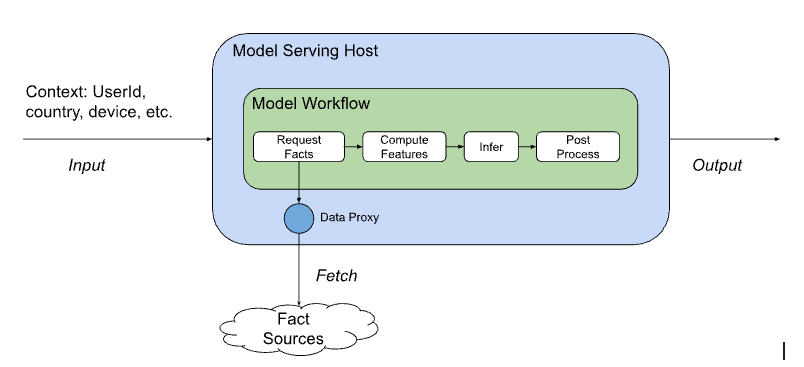
To properly frame our discussion, let’s first clarify the distinction between model serving and model inference. At Netflix, the definition of an ML model has historically been somewhat unique. While model inference typically focuses only on an infer(features) -> score capability, models at Netflix act as self-contained workflows that transform inputs to outputs. A “model” encapsulates pre- and post-processing, feature computation logic, and an optional ML-trained component, all packaged in a standard format suitable for use across multiple contexts. We refer to the end-to-end execution of this workflow as model serving. This distinction matters because our routing and API abstractions operate at the level of workflows, not just individual scoring functions.
A few simplified examples of model serving use cases:
Use case: Personalized Continue Watching row on Netflix Homepage
Input: UserId, Country, Device ID
Output: Ranked List of movies and shows (aka title): [titleId1, titleId2, titleId3,…]
Output: Probability of the transaction being fraudulent
A typical flow of this serving workflow is depicted below:
To achieve this higher level of abstraction, the model definition contains a list of facts (raw, unprocessed data or observations built as states in different business workflows) that it needs to compute features, and it relies on the model serving platform to supply these facts at serving time by calling several other microservices. Likewise, during offline training, Netflix’s ML fact store provides snapshots for bulk access to facilitate feature computation.
The important takeaway from this model definition is that the calling services only need to provide standard request context (such as userId, country, device), and the relevant domain context (such as titles to rank, or payment transaction for fraud detection), and the model can itself compute features and perform inference as part of the execution flow. This common set of request contexts across domains enables them to share a standard API abstraction and standardizes how various client microservices can uniformly integrate with the serving app. Furthermore, clients are shielded from the model selection and execution, allowing the model architecture and data inputs to evolve with minimal client coordination.
This post focuses on showcasing the technical details to support this design paradigm. We’ll first describe how we implemented this abstraction with Switchboard, a centralized routing service, and then discuss the operational challenges we encountered at scale and how they led us to the Lightbulb architecture.
ML Model Serving Platform Principles
We envisioned a central model serving platform for all of Netflix’s member-facing ML Model serving needs. This ambitious effort required principled thinking to provide the right level of abstraction for both the researchers and client applications. The following ideas, which are relevant to the topic of this blog post, ensured that the platform acts as an enabler of rapid ML innovation and limits the exposure of ML model iterations to the client apps:
Model innovation independent of client apps: There should be only a one-time integration effort by the calling app with the ML serving platform for a new use case. After that, almost all model iterations, including intermediate model A/B experiments, should be mostly opaque to the calling apps. This implies that the platform should handle tasks such as model selection based on a user’s A/B allocation, fetching additional data needed by experimental models, logging for further training or observability, and more. This also benefits the ML researcher, as they only need to coordinate with one platform for model innovation.
Decouple clients from model sharding: Models are distributed across multiple serving compute cluster shards, each with its own Virtual IP (VIP) Address. Various factors, such as traffic patterns, SLAs, model architecture, and CPU/Memory availability, affect model-to-cluster mapping, and changes to this mapping result in changes to the VIP address at which a model is reachable. The serving platform should make clients agnostic to such frequent VIP address changes while ensuring high availability.
Flexible traffic routing rules: Support flexible mechanisms to introduce new traffic routing rules. This includes supporting traffic routing based on A/B experiments, providing a knob to slowly shift traffic to new models and VIP addresses, and allowing client overrides.
Introducing Switchboard
Standard out-of-the-box API Gateway solutions (such as AWS API Gateway, a standalone Service Mesh proxy) did not meet all our requirements. In particular, we needed first-class integration with Netflix’s experimentation platform, the ability to expose gRPC endpoints to clients, and the ability to use rich domain-specific context for routing customizations, which generic proxies were not designed to handle. Furthermore, the platform required customizations to model-specific lifecycle stages (shadow mode, canaries, rollbacks) to enable safe rollouts and migrations.
Hence, we embarked on building a custom service that serves as a flexible proxy layer for all traffic, handling over 1 million requests per second while maintaining high availability and reliability. We named it Switchboard.
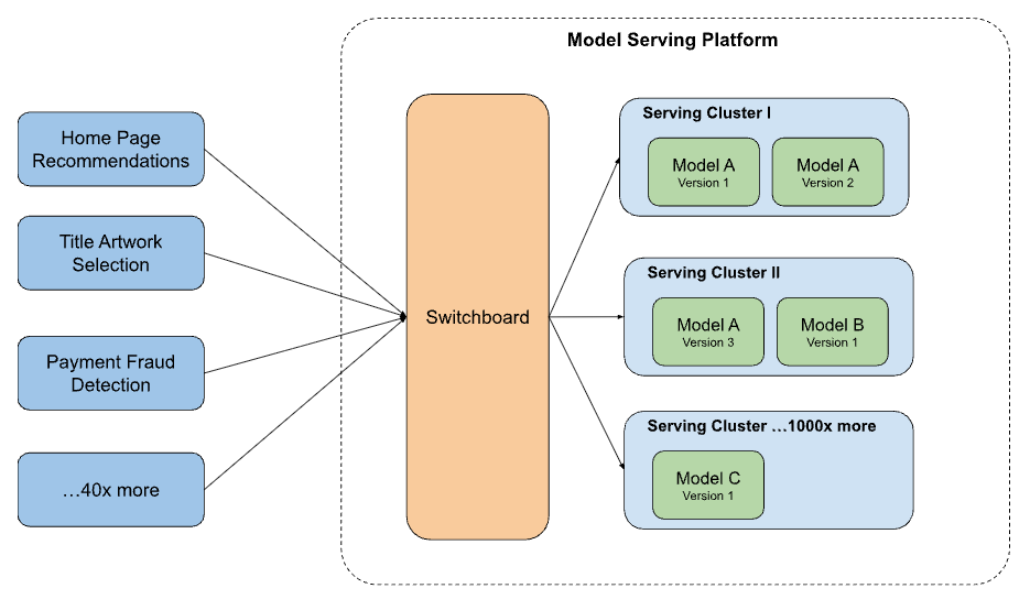
Switchboard serves as the central entry point for the system, acting as a mandatory interface for all clients to access the appropriate model based on their context. Its role is to perform context-aware routing and to apply any configured context enrichment to the model inputs.
Here is a visual representation of the request flow from different clients to different serving clusters:
Objective Abstraction
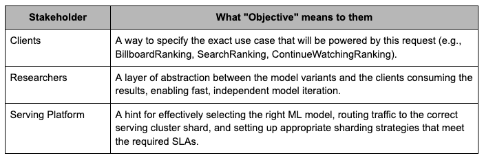
To support this system design, we introduce the concept of an “Objective”. It’s an Enumeration defined by the serving platform that every request into the system must provide. It has three key purposes:
In short, an Objective is the serving platform’s name for a specific business use case (e.g., ContinueWatchingRanking), which decouples clients from concrete models and guides the platform’s routing and model selection decisions.
Key Capabilities of Switchboard
To summarize, these are the key capabilities of Switchboard:
Common Client Abstraction: Switchboard provides a single point of contact for all our clients’ model needs. When clients wish to consume additional models for new ML applications addressing the same business need, there is no new service dependency to introduce or new clients to manage to make requests to the models. From an ML Ops perspective, this also gives us knobs to control client rate limits across model versions and manage central concurrency limits to deal with bad clients.
Context-Aware Routing: Switchboard can route a request based on a rich set of contextual features, such as the user’s current device, locale, ranking surface type (e.g., home page vs. search results), or the current A/B test a user is in.
Dynamic Traffic Splitting: It enables real-time traffic splitting for canary deployments and experimentation. This allows engineers to safely roll out a new model version to a small, controlled percentage of users before a full launch.
Model Versioning and Lifecycle Management: Switchboard inherently manages concurrent request traffic to multiple versions of the same model. This is crucial for:
Shadow Mode Testing: Routing production traffic to a new model version without affecting the user experience, enabling performance comparisons.
Instant Rollback: Immediate switching of traffic away from a problematic new model version back to a stable one.
But is this the whole story? Not quite. Introducing this routing layer adds complexity to our model deployment cycles. In addition, we need a mechanism to collect the context-based routing information from the researchers when they choose to deploy model variants.
The Glue — Switchboard Rules
Given that Objectives serve as the contract between clients and the serving platform, we needed a way for researchers to attach model variants, experiments, and traffic splits to those Objectives without changing client code. This is where Switchboard Rules comes in.
The primary UX for model researchers to define models associated with an objective in a flexible manner is a JavaScript configuration, which we call Switchboard Rules. It’s used to produce a set of rules (typically a JSON file) that primarily dictate the following things to the serving platform:
The default model to use for a given Objective
A/B experiments to configure for a set of Objectives and the corresponding models to load for those experiments
Customizations to gradually shift traffic to a new model
Here is an example of an A/B test rule in the context of the Continue Watching row:
/** Configuration rule written by a Model Researcher to add an A/B experiment in the Model Serving system. Cell 1: Uses the default, currently productized model Cell 2 and Cell 3: Use different experimental (candidate) models **/
function defineAB12345Rule() { const abTestId = 12345;
These rules are consumed by both the Switchboard and the Model Serving clusters. Given these rules, the serving platform components can take various actions, some detailed below:
Control Plane Flow:
Assignment: Produce model-to-cluster shard assignment.
Validation: Load all specified models into the Serving Cluster Shard and validate model dependencies to ensure successful execution.
Mapping: Provide the model-to-shard VIP address mapping to Switchboard.
Data Plane Flow:
Allocation: If the request is for Objective=ContinueWatchingRanking, query the Experimentation Platform for the userId’s cell allocation.
Model Selection: Use the allocation and A/B test rule to select the appropriate model.
Request Routing: Route the request to the serving cluster shard with the selected model and context.
Model Execution (on the serving host): Run the model workflow steps and return the response.
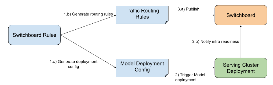
A key highlight of this setup is the decoupling of the experimentation config from the serving platform code. This includes having an independent release cycle for the rules, separate from the code deployments. Netflix’s Gutenberg system provides an excellent ecosystem that enables a flexible pub-sub architecture, facilitating proper versioning, dynamic loading, easy rollbacks, and more. Both Switchboard and the Serving Cluster Host subscribe to the same Switchboard Rules configuration.
To prevent race conditions and ensure proper sync of the dynamic Switchboard Rules configuration, the following flow is considered:
Evolving Challenges
Switchboard solved the primary problem of improving model iteration and innovation velocity, and provided an excellent ML serving abstraction to over 30 service clients. However, as the system scale increased, a few challenges and problems with this design became apparent:
Single point of failure: The presence of Switchboard in the critical request path clearly highlights the risks of shutting down access to all serving hosts in extreme cases, such as unintentional bugs or noisy neighbors sending excessive traffic.
Why this matters: Switchboard became a shared dependency whose failure would degrade or disable multiple ML-powered experiences at Netflix.
Added latency due to additional network hop: Switchboard in the request path adds between 10–20ms of latency due to serialization-deserialization operations, depending on payload size. Additionally, it further exposes a request to tail latency amplification.
Why this matters: The added latency is unacceptable for some latency-sensitive clients, resulting in end-user impact due to service timeouts.
Reduced Client flexibility: Switchboard obscures visibility into client request origins from the serving clusters. Consequently, distinguishing data logged for real vs artificial traffic, which is essential for model training, is difficult and requires ongoing customization and increased MLOps overhead.
Why this matters: It makes it harder to do tenant separation and test traffic isolation.
What Next? — Lightbulb
The aforementioned challenges of operating Switchboard at scale forced us to rethink the core implementation while retaining its key features. Our goal was not to throw away Switchboard’s design, but to refactor where and how its responsibilities were executed, keeping the benefits while reducing risk and latency. Particularly:
Common Client Abstraction
Decouple clients from model sharding
Flexible traffic routing rules
Lightweight system client
Single place to define model and experimentation config
Fast experimentation config propagation
Fallback and client-side caching in case of failures
However, we did want to address some of the previous design choices to move forward with:
Remove the routing service from the direct request path: Having a single service in the active request path introduces another failure mode and limits fallback flexibility. While routing rules change infrequently, maintaining consistency comes at the cost of increased availability risks.
Separate model inputs from the request metadata: In certain cases, the request payload could be quite large. Needing to deserialize and then re-serialize the payload as it flowed through Switchboard to make a routing decision was a significant contributor to latency and increased serving costs.
Provide better isolation for the routing layer: Consolidating multiple use cases (tenants) into a single routing cluster poses two main challenges. First, error propagation posed a risk, as a surge of problematic requests from one tenant could cascade errors back to Switchboard, potentially impacting other users. Second, the cluster had to accommodate diverse latency requirements because the requests from different use cases varied significantly in complexity.
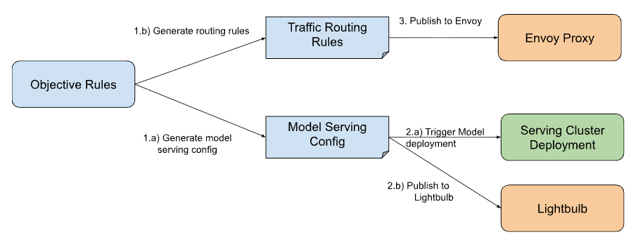
This required some changes in our setup flow: While it largely remained unchanged, however, we created separate components for Routing and Model Selection (Lightbulb):
We now take the rules for an Objective and break them into distinct sets of configuration:
Model Serving Configuration: This allows us to determine which model should be used at request time, along with the required metadata
Routing Rules: Given a model we want to serve at request time, this tells us which VIP the request should be routed to.
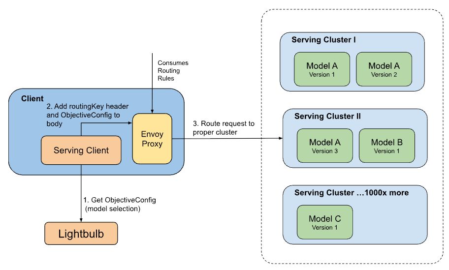
The Data Plane changes also reflect this separation, as we now rely on Envoy to take care of the routing details:
Envoy is already used for all egress communication between apps at Netflix, and it can route requests to different clusters (VIPs) based on the configurable Routing Rules published from our control plane. However, it lacks the information needed to make routing decisions and the ability to enrich the request body with additional serving parameters required for A/B testing model variants. We introduced Lightbulb to cover this gap:
Lightbulb consumes the minimal request context, which contains use-case information, and provides the metadata mapping required for routing at the Envoy layer.
Lightbulb resolves the request context to determine a routingKey configuration along with the ObjectiveConfig — this is where we place the model id along with other request-specific configurations required for model execution. This is done to separate the config resolution associated with the request from the placement and routing information needed to reach it on the inference cluster.
While the routingKey is added to the headers for Envoy proxy to consume, the client adds the ObjectiveConfig parameters to the request itself. This is done to avoid bloating the request headers while passing additional parameters for the model to process the request appropriately.
The routing of the actual request is performed by the Envoy proxy, which has the metadata to map the routingKey to the actual cluster VIP running the model. Because the routingKey is in a header, this determination can be made with minimal overhead.
These changes retain the advantages of Switchboard, such as a single integration point, abstraction of model id from use case, context-aware routing, while addressing the challenges we observed over time.
Conclusion
The evolution from Switchboard to Lightbulb marks a significant architectural refinement in our ML model serving infrastructure. While Switchboard provided the initial abstraction layer critical for rapid innovation, its latency and single-point-of-failure risk posed scaling hurdles. The subsequent adoption of Lightbulb, a decoupled service focused solely on routing metadata, and its integration with Envoy successfully resolved these challenges. This sophisticated new architecture preserves the key benefits — seamless client integration and flexible experimentation — while ensuring reliable, efficient, and scalable delivery of personalized member experiences, positioning us well for future ML growth.
In future posts in this series, we’ll dive deeper into other aspects of our ML serving platform, including inference and feature fetching, and how they interact with the routing architecture described here.
Special thanks to Sura Elamurugu, Sri Krishna Vempati, Ed Maddox, and Sreepathi Prasanna for their invaluable feedback and partnership in iterating on this idea and bringing this blog post to life.
Did you know that, at GitHub, we host all of our own source code on github.com? We do this because we’re our own biggest customer—testing out changes internally before they go to users. However, there’s one downside: If github.com were ever to go down, we wouldn’t be able to access our own source code.
This is what you’d call a very simple circular dependency: to deploy GitHub, we needed GitHub. If GitHub is down, then we wouldn’t be able to deploy something to fix it. We mitigate this by maintaining a mirror of our code for fixing forward and built assets for rolling back.
So we’re done, right? Problem solved? Nope, there are more circular dependencies to consider. For example, how do you stop a deployment script introducing a circular dependency of its own on an internal service or downloading a binary from GitHub?
When we started to design our new host-based deployment system, we evaluated some new approaches to prevent deployment code from creating circular dependencies. We found that using eBPF, we could selectively monitor and block those calls. In this blog post, we’ll take you through our findings and show how you can get started writing your own eBPF programs.
Types of circular dependencies
Let’s start by looking at the types of circular dependencies through a hypothetical scenario.
Suppose a MySQL outage occurs, which causes GitHub to be unable to serve release data from repositories. To resolve the incident, we need to roll out a configuration change to the stateful MySQL nodes that are impacted. This configuration change is applied by executing a deploy script on each node.
Now, let’s look at the different types of circular dependencies that could impact GitHub during this scenario.
Direct dependency: The MySQL deploy script attempts to pull the latest release of an open source tool from GitHub. Since GitHub can’t serve the release data (due to the outage), the script can’t complete.
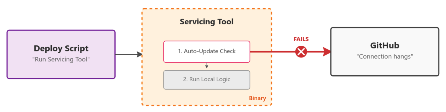
Hidden dependencies: The MySQL deploy script uses a servicing tool that is already present on the machine’s disk. However, when the tool runs, it checks GitHub to see if an update is available. If it’s unable to contact GitHub (due to the outage), the script may fail or hang, depending on how the tool handles the error when checking for updates.
Transient dependencies: The MySQL deploy script calls, via an API, another internal service (for example, a migrations service), which in turn attempts to fetch the latest release of an open source tool from GitHub to use the new binary. The failure propagates back to the deploy script.
How do you solve these circular dependencies?
Until recently, the onus has been on every team who that owns stateful hosts to review their deployment scripts and identify circular dependencies.
In practice, however, many dependencies aren’t identified until an incident occurs, which can delay recovery.
The obvious route would be to block access to github.com from the machines to validate that the system can deploy without it. But these hosts are stateful and serve customer traffic even during rolling deploys, drains, or restarts. Blocking github.com entirely would impact their ability to handle production requests.
This is where we started to look at eBPF, which lets you load custom programs into the Linux kernel and hook into core system primitives like networking.
A cGroup is a Linux primitive (used heavily by Docker but not limited to it) that enforces resource limits and isolation for sets of processes. You can create a cGroup, configure it, and move processes into it—no Docker required.
This started to look very promising. Could we create a cGroup, place only the deployment script inside it, and then limit the outbound network access of only that script? It certainly looked possible, so we started to build a proof of concept.
Building out per-process conditional network filtering with eBPF
We started on a proof of concept in go that used the cilium/ebpf library.
ebpf-go is a pure-Go library to read, modify, and load eBPF programs and attach them to various hooks in the Linux kernel.
It massively simplifies the process of authoring, building, and running programs that use eBPF. For example, to hook the BPF_PROG_TYPE_CGROUP_SKB program type, we can do this as follows: 👇
//go:generate go tool bpf2go -tags linux bpf cgroup_skb.c -- -I../headers
func main() {
// Load pre-compiled programs and maps into the kernel.
objs := bpfObjects{}
if err := loadBpfObjects(&objs, nil); err != nil {
log.Fatalf("loading objects: %v", err)
}
defer objs.Close()
// Link the count_egress_packets program to the cgroup.
l, err := link.AttachCgroup(link.CgroupOptions{
Path: "/sys/fs/cgroup/system.slice",
Attach: ebpf.AttachCGroupInetEgress,
Program: objs.CountEgressPackets,
})
if err != nil {
log.Fatal(err)
}
defer l.Close()
log.Println("Counting packets...")
// Read loop reporting the total amount of times the kernel
// function was entered, once per second.
ticker := time.NewTicker(1 * time.Second)
defer ticker.Stop()
for range ticker.C {
var value uint64
if err := objs.PktCount.Lookup(uint32(0), &value); err != nil {
log.Fatalf("reading map: %v", err)
}
log.Printf("number of packets: %d\n", value)
}
}
The //go:generate line handles compiling the eBPF C code and auto-generating the bpfObjects struct, which allows us to attach and interact with the program. This means a simple go build is all you need. 🥳
There was still a missing piece though: CGROUP_SKB operates on IP addresses. Given the breadth of GitHub’s systems and rate of change, keeping an up-to-date block IP list would be very hard.
Could we use more eBPF to create a DNS-based blocked list? Yes, it turns out we could.
Here is a simplified example where we rewrite any connect4 syscall targeting DNS (Port 53) to localhost:53.
cgroupLink, err := link.AttachCgroup(link.CgroupOptions{
Path: cgroup.Name(),
Attach: ebpf.AttachCGroupInet4Connect,
Program: obj.Connect4,
})
if err != nil {
return nil, fmt.Errorf("attaching eBPF program Connect4 to cgroup: %w", err)
}
/* This is the hexadecimal representation of 127.0.0.1 address */
const __u32 ADDRESS_LOCALHOST_NETBYTEORDER = bpf_htonl(0x7f000001);
SEC("cgroup/connect4")
int connect4(struct bpf_sock_addr *ctx) {
__be32 original_ip = ctx->user_ip4;
__u16 original_port = bpf_ntohs(ctx->user_port);
if (ctx->user_port == bpf_htons(53)) {
/* For DNS Query (*:53) rewire service to backend
* 127.0.0.1:const_dns_proxy_port */
ctx->user_ip4 = const_mitm_proxy_address;
ctx->user_port = bpf_htons(const_dns_proxy_port);
}
return 1;
}
We used this to intercept DNS queries from the cGroup and forward them to a userspace DNS proxy we run.
Now, any DNS queries initiated by the deployment script are routed through our DNS proxy. Our proxy evaluates each requested domain against our block list and uses eBPF Maps to communicate with the CGROUP_SKB program, allowing or denying the request accordingly.
If you’d like to dig into the code, here’s an early proof of concept we put together. Our current implementation has progressed since then, but this should serve as a good intro.
Like any fun project, the deeper we got, the more we realized we could do.
For example, could we correlate blocked DNS requests back to the specific command or process that triggered them, so teams could more easily debug and fix issues? Yes, we can!
As we’re redirecting all DNS calls to our userspace DNS proxy, we can look at the transaction ID of each request, find the domain being resolved, and lookup in the eBPF Map to see which process made the request. By reading /proc/{PID}/cmdline, we can even extract the full command line that triggered the request.
Then we can output a log line with all the information:
Conditionally block domains that would cause circular dependencies from deployment scripts.
Inform the owning team which command triggered the blocked request.
Provide an audit list of all domains contacted during a deployment.
Use the cGroups to enforce CPU and memory limits on deploy scripts, preventing runaway resource usage from impacting workloads.
What’s next?
Our new circular dependency detection process is live after a six-month rollout.
Now, if a team accidentally adds a problematic dependency, or if an existing binary tool we use takes a new dependency, the tooling will detect that problem and flag it to the team.
The net result is a more stable GitHub and faster mean time to recovery during incidents (due to the removal of these circular dependencies).
Are there ways for circular dependencies to still trip things up? You bet—and we’ll look to improve the tool as we discover them.
Want to dive in?
Has this piqued your interest in what you might be able to do with eBPF?
Get started by having a look through the examples in cilium/ebpf and the great documentation on the docs.ebpf.io site.
An agent needs to be powered by a large language model. A few weeks ago, we announced that Workers AI is officially entering the arena for hosting large open-source models like Moonshot’s Kimi K2.5. Since then, we’ve made Kimi K2.5 3x faster and have more model additions in-flight. These models have been the backbone of a lot of the agentic products, harnesses, and tools that we have been launching this week.
Hosting AI models is an interesting challenge: it requires a delicate balance between software and very, very expensive hardware. At Cloudflare, we’re good at squeezing every bit of efficiency out of our hardware through clever software engineering. This is a deep dive on how we’re laying the foundation to run extra-large language models.
Hardware configurations
As we mentioned in our previous Kimi K2.5 blog post, we’re using a variety of hardware configurations in order to best serve models. A lot of hardware configurations depend on the size of inputs and outputs that users are sending to the model. For example, if you are using a model to write fanfiction, you might give it a few small prompts (input tokens) while asking it to generate pages of content (output tokens).
Conversely, if you are running a summarization task, you might be sending in hundreds of thousands of input tokens, but only generating a small summary with a few thousand output tokens. Presented with these opposing use cases, you have to make a choice — should you tune your model configuration so it’s faster at processing input tokens, or faster at generating output tokens?
When we launched large language models on Workers AI, we knew that most of the use cases would be used for agents. With agents, you send in a large number of input tokens. It starts off with a large system prompt, all the tools, MCPs. With the first user prompt, that context keeps growing. Each new prompt from the user sends a request to the model, which consists of everything that was said before — all the previous user prompts, assistant messages, code generated, etc. For Workers AI, that means we had to focus on two things: fast input token processing and fast tool calling.
Prefill decode (PD) disaggregation
One hardware configuration that we use to improve performance and efficiency is disaggregated prefill. There are two stages to processing an LLM request: prefill, which processes the input tokens and populates the KV cache, and decode, which generates output tokens. Prefill is usually compute bound, while decode is memory bound. This means that the parts of the GPU that are used in each stage are different, and since prefill is always done before decode, the stages block one another. Ultimately, it means that we are not efficiently utilizing all of our GPU power if we do both prefill and decode on a single machine.
With prefill decode disaggregation, separate inference servers are run for each stage. First, a request is sent to the prefill stage which performs prefill and stores it in its KV cache. Then the same request is sent to the decode server, with information about how to transfer the KV cache from the prefill server and begin decoding. This has a number of advantages, because it allows the servers to be tuned independently for the role they are performing, scaled to account for more input-heavy or output-heavy traffic, or even to run on heterogeneous hardware.
This architecture requires a relatively complex load balancer to achieve. Beyond just routing the requests as described above, it must rewrite the responses (including streaming SSE) of the decode server to include information from the prefill server such as cached tokens. To complicate matters, different inference servers require different information to initiate the KV cache transfer. We extended this to implement token-aware load balancing, in which there is a pool of prefill and decode endpoints, and the load balancer estimates how many prefill or decode tokens are in-flight to each endpoint in the pool and attempts to spread this load evenly.
After our public model launch, our input/output patterns changed drastically again. We took the time to analyze our new usage patterns and then tuned our configuration to fit our customer’s use cases.
Here’s a graph of our p90 Time to First Token drop after shifting traffic to our new PD disaggregated architecture, whilst request volume increased, using the same quantity of GPUs. We see a significant improvement in the tail latency variance.
Similarly, p90 time per token went from ~100 ms with high variance to 20-30 ms, a 3x improvement in intertoken latency.
Prompt Caching
Since agentic use cases usually have long contexts, we optimize for efficient prompt caching in order to not recompute input tensors on every turn. We leverage a header called x-session-affinity in order to help requests route to the right region that previously had the computed input tensors. We wrote about this in our original blog post about launching large LLMs on Workers AI. We added session affinity headers to popular agent harnesses like OpenCode, where we noticed a significant increase in total throughput. A small difference in prompt caching from our users can sum to a factor of additional GPUs needed to run a model. While we have KV-aware routing internally, we also rely on clients sending the x-session-affinity in order to be explicit about prompt caching. We incentivize the use of the header by offering discounted cached tokens. We highly encourage users to leverage prompt caching in order to have faster inference and cheaper pricing.
We worked with our heaviest internal users to adopt this header. The result was an increase in input token cache hit ratios from 60% to 80% during peak times. This significantly increases the request throughput that we can handle, while offering better performance for interactive or time-sensitive sessions like OpenCode or AI code reviews.
KV-cache optimization
As we’re serving larger models now, one instance can span multiple GPUs. This means that we had to find an efficient way to share KV cache across GPUs. KV cache is where all the input tensors from prefill (result of prompts in a session) are stored, and initially lives in the VRAM of a GPU. Every GPU has a fixed VRAM size, but if your model instance requires multiple GPUs, there needs to be a way for the KV cache to live across GPUs and talk to each other. To achieve this for Kimi, we leveraged Moonshot AI’s Mooncake Transfer Engine and Mooncake Store.
Mooncake’s Transfer Engine is a high-performance data transfer framework. It works with different Remote Direct Memory Access (RDMA) protocols such as NVLink and NVMe over Fabric, which enables direct memory-to-memory data transfer without involving the CPU. It improves the speed of transferring data across multiple GPU machines, which is particularly important in multi-GPU and multi-node configurations for models.
When paired with LMCache or SGLang HiCache, the cache is shared across all nodes in the cluster, allowing a prefill node to identify and re-use a cache from a previous request that was originally pre-filled on a different node. This eliminates the need for session aware routing within a cluster and allows us to load balance the traffic much more evenly. Mooncake Store also allows us to extend the cache beyond GPU VRAM, and leverage NVMe storage. This extends the time that sessions remain in cache, improving our cache hit ratio and allowing us to handle more traffic and offer better performance to users.
Speculative decoding
LLMs work by predicting the next token in a sequence, based on the tokens that came before it. With a naive implementation, models only predict the next n token, but we can actually make it predict the next n+1, n+2… tokens in a single forward pass of the model. This popular technique is known as speculative decoding, which we’ve written about in a previous post on Workers AI.
With speculative decoding, we leverage a smaller LLM (the draft model) to generate a few candidate tokens for the target model to choose from. The target model then just has to select from a small pool of candidate tokens in a single forward pass. Validating the tokens is faster and less computationally expensive than using the larger target model to generate the tokens. However, quality is still upheld as the target model ultimately has to accept or reject the draft tokens.
In agentic use cases, speculative decoding really shines because of the volume of tool calls and structured outputs that models need to generate. A tool call is largely predictable — you know there will be a name, description, and it’s wrapped in a JSON envelope.
To do this with Kimi K2.5, we leverage NVIDIA’s EAGLE-3 (Extrapolation Algorithm for Greater Language-model Efficiency) draft model. The levers for tuning speculative decoding include the number of future tokens to generate. As a result, we’re able to achieve high-quality inference while speeding up tokens per second throughput.
Infire: our proprietary inference engine
As we announced during Birthday Week in 2025, Cloudflare has a proprietary inference engine, Infire, that makes machine learning models faster. Infire is an inference engine written in Rust, designed to support Cloudflare’s unique challenges with inference given our distributed global network. We’ve extended Infire support for this new class of large language models we are planning to run, which meant we had to build a few new features to make it all work.
Multi-GPU support
Large language models like Kimi K2.5 are over 1 trillion parameters, which is about 560GB of model weights. A typical H100 has about 80GB of VRAM and the model weights need to be loaded in GPU memory in order to run. This means that a model like Kimi K2.5 needs at least 8 H100s in order to load the model into memory and run — and that’s not even including the extra VRAM you would need for KV Cache, which includes your context window.
Since we initially launched Infire, we had to add support for multi-GPU, letting the inference engine run across multiple GPUs in either pipeline-parallel or tensor-parallel modes with expert-parallelism supported as well.
For pipeline parallelism, Infire attempts to properly load balance all stages of the pipeline, in order to prevent the GPUs of one stage from starving while other stages are executing. On the other hand, for tensor parallelism, Infire optimizes for reducing cross-GPU communication, making it as fast as possible. For most models, utilizing both pipeline parallelism and tensor parallelism in tandem provides the best balance of throughput and latency.
Even lower memory overhead
While already having much lower GPU memory overhead than vLLM, we optimized Infire even further, tightening the memory required for internal state like activations. Currently Infire is capable of running Llama 4 Scout on just two H200 GPUs with more than 56 GiB remaining for KV-cache, sufficient for more than 1.2m tokens. Infire is also capable of running Kimi K2.5 on 8 H100 GPUs (yes that is H100), with more than 30 GiB still available for KV-cache. In both cases you would have trouble even booting vLLM in the first place.
Faster cold-starts
While adding multi-GPU support, we identified additional opportunities to improve boot times. Even for the largest models, such as Kimi K2.5, Infire can begin serving requests in under 20 seconds. The load times are only bounded by the drive speed.
Maximizing our hardware for faster throughput
Investing in our proprietary inference engine enables us to maximize our hardware by getting up to 20% higher tokens per second throughput on unconstrained systems, and also enabling us to use lower-end hardware to run the latest models, where it was previously completely infeasible.
The journey doesn’t end
New technologies, research, and models come out on a weekly basis for the machine learning community. We’re continuously optimizing our technology stack in order to provide high-quality, performant inference for our customers while operating our GPUs efficiently. If these sound like interesting challenges for you – we’re hiring!
Every time we restarted Atlantis, the tool we use to plan and apply Terraform changes, we’d be stuck for 30 minutes waiting for it to come back up. No plans, no applies, no infrastructure changes for any repository managed by Atlantis. With roughly 100 restarts a month for credential rotations and unboarding, that added up to over 50 hours of blocked engineering time every month, and paged the on-call engineer every time.
This was ultimately caused by a safe default in Kubernetes that had silently become a bottleneck as the persistent volume used by Atlantis grew to millions of files. Here’s how we tracked it down and fixed it with a one-line change.
Mysteriously slow restarts
We manage dozens of Terraform projects with GitLab merge requests (MRs) using Atlantis, which handles planning and applying. It enforces locking to ensure that only one MR can modify a project at a time.
It runs on Kubernetes as a singleton StatefulSet and relies on a Kubernetes PersistentVolume (PV) to keep track of repository state on disk. Whenever a Terraform project needs to be onboarded or offboarded, or credentials used by Terraform are updated, we have to restart Atlantis to pick up those changes — a process that can take 30 minutes.
The slow restart was apparent when we recently ran out of inodes on the persistent storage used by Atlantis, forcing us to restart it to resize the volume. Inodes are consumed by each file and directory entry on disk, and the number available to a filesystem is determined by parameters passed when creating it. The Ceph persistent storage implementation provided by our Kubernetes platform does not expose a way to pass flags to mkfs, so we’re at the mercy of default values: growing the filesystem is the only way to grow available inodes, and restarting a PV requires a pod restart.
We talked about extending the alert window, but that would just mask the problem and delay our response to actual issues. Instead, we decided to investigate exactly why it was taking so long.
Bad behavior
When we were asked to do a rolling restart of Atlantis to pick up a change to the secrets it uses, we would run kubectl rollout restart statefulset atlantis, which would gracefully terminate the existing Atlantis pod before spinning up a new one. The new pod would appear almost immediately, but looking at it would show:
$ kubectl get pod atlantis-0
atlantis-0 0/1
Init:0/1 0 30m
…so what gives? Naturally, the first thing to check would be events for that pod. It’s waiting around for an init container to run, so maybe the pod events would illuminate why?
$ kubectl events --for=pod/atlantis-0
LAST SEEN TYPE REASON OBJECT MESSAGE
30m Normal Killing Pod/atlantis-0 Stopping container atlantis-server
30m Normal Scheduled Pod/atlantis-0 Successfully assigned atlantis/atlantis-0 to 36com1167.cfops.net
22s Normal Pulling Pod/atlantis-0 Pulling image "oci.example.com/git-sync/master:v4.1.0"
22s Normal Pulled Pod/atlantis-0 Successfully pulled image "oci.example.com/git-sync/master:v4.1.0" in 632ms (632ms including waiting). Image size: 58518579 bytes.
That looks almost normal… but what’s taking so long between scheduling the pod and actually starting to pull the image for the init container? Unfortunately that was all the data we had to go on from Kubernetes itself. But surely there had to be something more that can tell us why it’s taking so long to actually start running the pod.
Going deeper
In Kubernetes, a component called kubelet that runs on each node is responsible for coordinating pod creation, mounting persistent volumes, and many other things. From my time on our Kubernetes team, I know that kubelet runs as a systemd service and so its logs should be available to us in Kibana. Since the pod has been scheduled, we know the host name we’re interested in, and the log messages from kubelet include the associated object, so we could filter for atlantis to narrow down the log messages to anything we found interesting.
We were able to observe the Atlantis PV being mounted shortly after the pod was scheduled. We also observed all the secret volumes mount without issue. However, there was still a big unexplained gap in the logs. We saw:
[operation_generator.go:664] "MountVolume.MountDevice succeeded for volume \"pvc-94b75052-8d70-4c67-993a-9238613f3b99\" (UniqueName: \"kubernetes.io/csi/rook-ceph-nvme.rbd.csi.ceph.com^0001-000e-rook-ceph-nvme-0000000000000002-a6163184-670f-422b-a135-a1246dba4695\") pod \"atlantis-0\" (UID: \"83089f13-2d9b-46ed-a4d3-cba885f9f48a\") device mount path \"/state/var/lib/kubelet/plugins/kubernetes.io/csi/rook-ceph-nvme.rbd.csi.ceph.com/d42dcb508f87fa241a49c4f589c03d80de2f720a87e36932aedc4c07840e2dfc/globalmount\"" pod="atlantis/atlantis-0"
[pod_workers.go:1298] "Error syncing pod, skipping" err="unmounted volumes=[atlantis-storage], unattached volumes=[], failed to process volumes=[]: context deadline exceeded" pod="atlantis/atlantis-0" podUID="83089f13-2d9b-46ed-a4d3-cba885f9f48a"
[util.go:30] "No sandbox for pod can be found. Need to start a new one" pod="atlantis/atlantis-0"
The last two messages looped several times until eventually we observed the pod actually start up properly.
So kubelet thinks that the pod is otherwise ready to go, but it’s not starting it and something’s timing out.
The missing piece
The lowest-level logs we had on the pod didn’t show us what’s going on. What else do we have to look at? Well, the last message before it hangs is the PV being mounted onto the node. Ordinarily, if the PV has issues mounting (e.g. due to still being stuck mounted on another node), that will bubble up as an event. But something’s still going on here, and the only thing we have left to drill down on is the PV itself. So I plug that into Kibana, since the PV name is unique enough to make a good search term… and immediately something jumps out:
[volume_linux.go:49] Setting volume ownership for /state/var/lib/kubelet/pods/83089f13-2d9b-46ed-a4d3-cba885f9f48a/volumes/kubernetes.io~csi/pvc-94b75052-8d70-4c67-993a-9238613f3b99/mount and fsGroup set. If the volume has a lot of files then setting volume ownership could be slow, see https://github.com/kubernetes/kubernetes/issues/69699
Remember how I said at the beginning we’d just run out of inodes? In other words, we have a lot of files on this PV. When the PV is mounted, kubelet is running chgrp -R to recursively change the group on every file and folder across this filesystem. No wonder it was taking so long — that’s a ton of entries to traverse even on fast flash storage!
The pod’s spec.securityContext included fsGroup: 1, which ensures that processes running under GID 1 can access files on the volume. Atlantis runs as a non-root user, so without this setting it wouldn’t have permission to read or write to the PV. The way Kubernetes enforces this is by recursively updating ownership on the entire PV every time it’s mounted.
The fix
Fixing this was heroically…boring. Since version 1.20, Kubernetes has supported an additional field on pod.spec.securityContext called fsGroupChangePolicy. This field defaults to Always, which leads to the exact behavior we see here. It has another option, OnRootMismatch, to only change permissions if the root directory of the PV doesn’t have the right permissions. If you don’t know exactly how files are created on your PV, do not set fsGroupChangePolicy: OnRootMismatch. We checked to make sure that nothing should be changing the group on anything in the PV, and then set that field:
Now, it takes about 30 seconds to restart Atlantis, down from the 30 minutes it was when we started.
Default Kubernetes settings are sensible for small volumes, but they can become bottlenecks as data grows. For us, this one-line change to fsGroupChangePolicy reclaimed nearly 50 hours of blocked engineering time per month. This was time our teams had been spending waiting for infrastructure changes to go through, and time that our on-call engineers had been spending responding to false alarms. That’s roughly 600 hours a year returned to productive work, from a fix that took longer to diagnose than deploy.
Safe defaults in Kubernetes are designed for small, simple workloads. But as you scale, they can slowly become bottlenecks. If you’re running workloads with large persistent volumes, it’s worth checking whether recursive permission changes like this are silently eating your restart time. Audit your securityContext settings, especially fsGroup and fsGroupChangePolicy. OnRootMismatch has been available since v1.20.
Not every fix is heroic or complex, and it’s usually worth asking “why does the system behave this way?”
Two years ago, Cloudflare deployed our 12th Generation server fleet, based on AMD EPYC™ Genoa-X processors with their massive 3D V-Cache. That cache-heavy architecture was a perfect match for our request handling layer, FL1 at the time. But as we evaluated next-generation hardware, we faced a dilemma — the CPUs offering the biggest throughput gains came with a significant cache reduction. Our legacy software stack wasn’t optimized for this, and the potential throughput benefits were being capped by increasing latency.
This blog describes how the FL2 transition, our Rust-based rewrite of Cloudflare’s core request handling layer, allowed us to prove Gen 13’s full potential and unlock performance gains that would have been impossible on our previous stack. FL2 removes the dependency on the larger cache, allowing for performance to scale with cores while maintaining our SLAs. Today, we are proud to announce the launch of Cloudflare’s Gen 13 based on AMD EPYC™ 5th Gen Turin-based servers running FL2, effectively capturing and scaling performance at the edge.
What AMD EPYCTurin brings to the table
AMD’s EPYC™ 5th Generation Turin-based processors deliver more than just a core count increase. The architecture delivers improvements across multiple dimensions of what Cloudflare servers require.
2x core count: up to 192 cores versus Gen 12’s 96 cores, with SMT providing 384 threads
Improved IPC: Zen 5’s architectural improvements deliver better instructions-per-cycle compared to Zen 4
Better power efficiency: Despite the higher core count, Turin consumes up to 32% fewer watts per core compared to Genoa-X
DDR5-6400 support: Higher memory bandwidth to feed all those cores
However, Turin’s high density OPNs make a deliberate tradeoff: prioritizing throughput over per core cache. Our analysis across the Turin stack highlighted this shift. For example, comparing the highest density Turin OPN to our Gen 12 Genoa-X processors reveals that Turin’s 192 cores share 384MB of L3 cache. This leaves each core with access to just 2MB, one-sixth of Gen 12’s allocation. For any workload that relies heavily on cache locality, which ours did, this reduction posed a serious challenge.
Generation
Processor
Cores/Threads
L3 Cache/Core
Gen 12
AMD Genoa-X 9684X
96C/192T
12MB (3D V-Cache)
Gen 13 Option 1
AMD Turin 9755
128C/256T
4MB
Gen 13 Option 2
AMD Turin 9845
160C/320T
2MB
Gen 13 Option 3
AMD Turin 9965
192C/384T
2MB
Diagnosing the problem with performance counters
For our FL1 request handling layer, NGINX- and LuaJIT-based code, this cache reduction presented a significant challenge. But we didn’t just assume it would be a problem; we measured it.
During the CPU evaluation phase for Gen 13, we collected CPU performance counters and profiling data to identify exactly what was happening under the hood using AMD uProf tool. The data showed:
L3 cache miss rates increased dramatically compared to Gen 12’s server equipped with 3D V-cache processors
Memory fetch latency dominated request processing time as data that previously stayed in L3 now required trips to DRAM
The latency penalty scaled with utilization as we pushed CPU usage higher, and cache contention worsened
L3 cache hits complete in roughly 50 cycles; L3 cache misses requiring DRAM access take 350+ cycles, an order of magnitude difference. With 6x less cache per core, FL1 on Gen 13 was hitting memory far more often, incurring latency penalties.
The tradeoff: latency vs. throughput
Our initial tests running FL1 on Gen 13 confirmed what the performance counters had already suggested. While the Turin processor could achieve higher throughput, it came at a steep latency cost.
Metric
Gen 12 (FL1)
Gen 13 – AMD Turin 9755 (FL1)
Gen 13 – AMD Turin 9845 (FL1)
Gen 13 – AMD Turin 9965 (FL1)
Delta
Core count
baseline
+33%
+67%
+100%
FL throughput
baseline
+10%
+31%
+62%
Improvement
Latency at low to moderate CPU utilization
baseline
+10%
+30%
+30%
Regression
Latency at high CPU utilization
baseline
> 20%
> 50%
> 50%
Unacceptable
The Gen 13 evaluation server with AMD Turin 9965 that generated 60% throughput gain was compelling, and the performance uplift provided the most improvement to Cloudflare’s total cost of ownership (TCO).
But a more than 50% latency penalty is not acceptable. The increase in request processing latency would directly impact customer experience. We faced a familiar infrastructure question: do we accept a solution with no TCO benefit, accept the increased latency tradeoff, or find a way to boost efficiency without adding latency?
Incremental gains with performance tuning
To find a path to an optimal outcome, we collaborated with AMD to analyze the Turin 9965 data and run targeted optimization experiments. We systematically tested multiple configurations:
Hardware Tuning: Adjusting hardware prefetchers and Data Fabric (DF) Probe Filters, which showed only marginal gains
Scaling Workers: Launching more FL1 workers, which improved throughput but cannibalized resources from other production services
CPU Pinning & Isolation: Adjusting workload isolation configurations to find optimal mix, with limited success
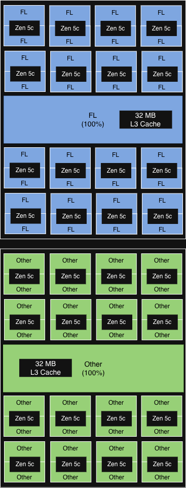
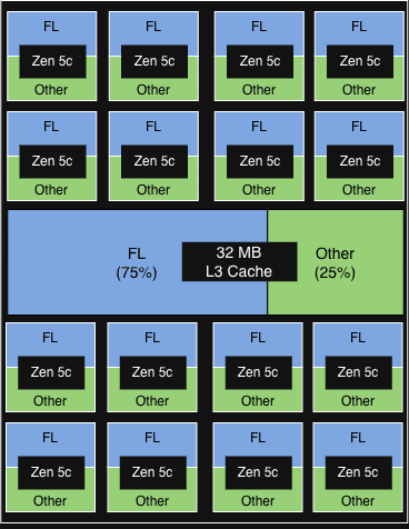
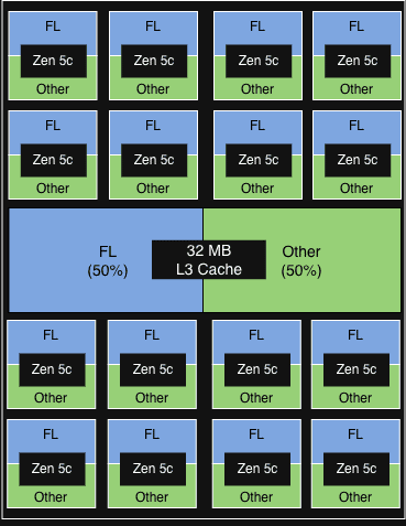
The configuration that ultimately provided the most value was AMD’s Platform Quality of Service (PQOS). PQOS extensions enable fine-grained regulation of shared resources like cache and memory bandwidth. Since Turin processors consist of one I/O Die and up to 12 Core Complex Dies (CCDs), each sharing an L3 cache across up to 16 cores, we put this to the test. Here is how the different experimental configurations performed.
First, we used PQOS to allocate a dedicated L3 cache share within a single CCD for FL1, the gains were minimal. However, when we scaled the concept to the socket level, dedicating an entire CCD strictly to FL1, we saw meaningful throughput gains while keeping latency acceptable.
Configuration
Description
Illustration
Performance gain
NUMA-aware core affinity (equivalent to PQOS at socket level)
6 out of 12 CCD (aligned with NUMA domain) run FL.
32MB L3 cache in each CCD shared among all cores.
>15% incremental
throughput gain
PQOS config 1
1 of 2 vCPU on each physical core in each CCD runs FL.
FL gets 75% of the 32MB L3 cache of each CCD.
< 5% incremental throughput gain
Other services show minor signs of degradation
PQOS config 2
1 of 2 vCPU in each physical core in each CCD runs FL.
FL gets 50% of the 32MB L3 cache of each CCD.
< 5% incremental throughput gain
PQOS config 3
2 vCPU on 50% of the physical core in each CCD runs FL.
FL gets 50% of the 32MB L3 cache of each CCD.
< 5% incremental throughput gain
The opportunity: FL2 was already in progress
Hardware tuning and resource configuration provided modest gains, but to truly unlock the performance potential of the Gen 13 architecture, we knew we would have to rewrite our software stack to fundamentally change how it utilized system resources.
Fortunately, we weren’t starting from scratch. As we announced during Birthday Week 2025, we had already been rebuilding FL1 from the ground up. FL2 is a complete rewrite of our request handling layer in Rust, built on our Pingora and Oxy frameworks, replacing 15 years of NGINX and LuaJIT code.
The FL2 project wasn’t initiated to solve the Gen 13 cache problem — it was driven by the need for better security (Rust’s memory safety), faster development velocity (strict module system), and improved performance across the board (less CPU, less memory, modular execution).
FL2’s cleaner architecture, with better memory access patterns and less dynamic allocation, might not depend on massive L3 caches the way FL1 did. This gave us an opportunity to use the FL2 transition to prove whether Gen 13’s throughput gains could be realized without the latency penalty.
Proving it out: FL2 on Gen 13
As the FL2 rollout progressed, production metrics from our Gen 13 servers validated what we had hypothesized.
Metric
Gen 13 AMD Turin 9965 (FL1)
Gen 13 AMD Turin 9965 (FL2)
FL requests per CPU%
baseline
50% higher
Latency vs Gen 12
baseline
70% lower
Throughput vs Gen 12
62% higher
100% higher
The out-of-the-box efficiency gains on our new FL2 stack were substantial, even before any system optimizations. FL2 slashed the latency penalty by 70%, allowing us to push Gen 13 to higher CPU utilization while strictly meeting our latency SLAs. Under FL1, this would have been impossible.
By effectively eliminating the cache bottleneck, FL2 enables our throughput to scale linearly with core count. The impact is undeniable on the high-density AMD Turin 9965: we achieved a 2x performance gain, unlocking the true potential of the hardware. With further system tuning, we expect to squeeze even more power out of our Gen 13 fleet.
Generational improvement with Gen 13
With FL2 unlocking the immense throughput of the high-core-count AMD Turin 9965, we have officially selected these processors for our Gen 13 deployment. Hardware qualification is complete, and Gen 13 servers are now shipping at scale to support our global rollout.
Performance improvements
Gen 12
Gen 13
Processor
AMD EPYC™ 4th Gen Genoa-X 9684X
AMD EPYC™ 5th Gen Turin 9965
Core count
96C/192T
192C/384T
FL throughput
baseline
Up to +100%
Performance per watt
baseline
Up to +50%
Gen 13 business impact
Up to 2x throughput vs Gen 12 for uncompromising customer experience: By doubling our throughput capacity while staying within our latency SLAs, we guarantee our applications remain fast and responsive, and able to absorb massive traffic spikes.
50% better performance/watt vs Gen 12 for sustainable scaling: This gain in power efficiency not only reduces data center expansion costs, but allows us to process growing traffic with a vastly lower carbon footprint per request.
60% higher rack throughput vs Gen 12 for global edge upgrades: Because we achieved this throughput density while keeping the rack power budget constant, we can seamlessly deploy this next generation compute anywhere in the world across our global edge network, delivering top tier performance exactly where our customers want it.
Gen 13 + FL2: ready for the edge
Our legacy request serving layer FL1 hit a cache contention wall on Gen 13, forcing an unacceptable tradeoff between throughput and latency. Instead of compromising, we built FL2.
Designed with a vastly leaner memory access pattern, FL2 removes our dependency on massive L3 caches and allows linear scaling with core count. Running on the Gen 13 AMD Turin platform, FL2 unlocks 2x the throughput and a 50% boost in power efficiency all while keeping latency within our SLAs. This leap forward is a great reminder of the importance of hardware-software co-design. Unconstrained by cache limits, Gen 13 servers are now ready to be deployed to serve millions of requests across Cloudflare’s global network.
If you’re excited about working on infrastructure at global scale, we’re hiring.
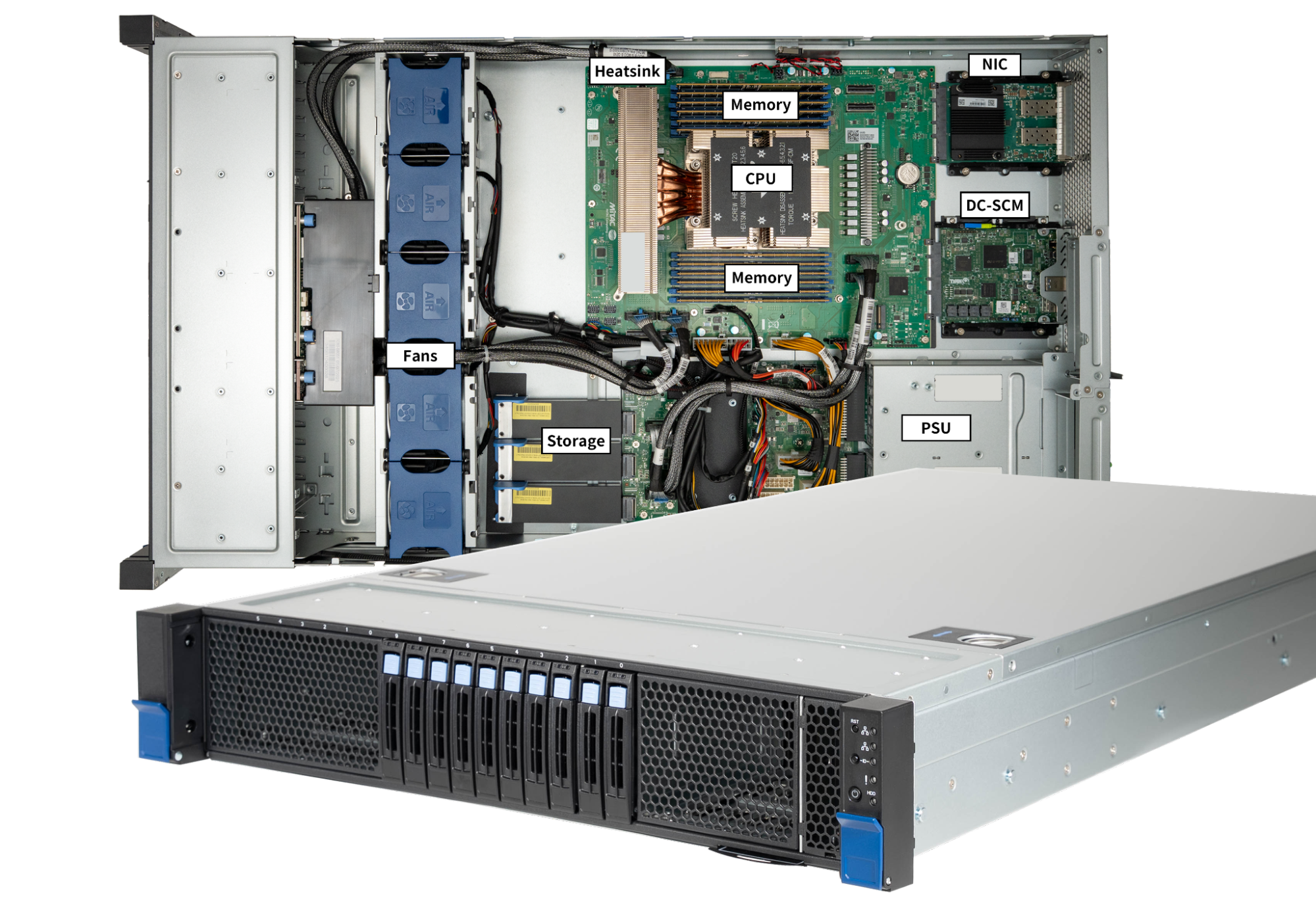
A few months ago, Cloudflare announced the transition to FL2, our Rust-based rewrite of Cloudflare’s core request handling layer. This transition accelerates our ability to help build a better Internet for everyone. With the migration in the software stack, Cloudflare has refreshed our server hardware design with improved hardware capabilities and better efficiency to serve the evolving demands of our network and software stack. Gen 13 is designed with 192-core AMD EPYC™ Turin 9965 processor, 768 GB of DDR5-6400 memory, 24 TB of PCIe 5.0 NVMe storage, and dual 100 GbE port network interface card.
Gen 13 delivers:
Up to 2x throughput compared to Gen 12 while staying within latency SLA
Up to 50% improvement in performance / watt efficiency, reducing data center expansion costs
Up to 60% higher throughput per rack keeping rack power budget constant
The three CPU candidates are designed to target different use cases: AMD Turin 9755 offers superior per-core performance, AMD Turin 9965 trades per-core performance for efficiency, and AMD Turin 9845 trades core count for lower socket power. We evaluated three CPUs in the production environment.
CPU Model
AMD Genoa-X 9684X
AMD Turin 9755
AMD Turin 9845
AMD Turin 9965
For server platform
Gen 12
Gen 13 candidate
Gen 13 candidate
Gen 13 candidate
# of CPU Cores
96
128
160
192
# of Threads
192
256
320
384
Base Clock
2.4 GHz
2.7 GHz
2.1 GHz
2.25 GHz
Max Boost Clock
3.7 GHz
4.1 GHz
3.7 GHz
3.7 GHz
All Core Boost Clock
3.42 GHz
4.1 GHz
3.25 GHz
3.35 GHz
Total L3 Cache
1152 MB
512 MB
320 MB
384 MB
L3 cache per core
12 MB / core
4 MB / core
2 MB / core
2 MB / core
Maximum configurable TDP
400W
500W
390W
500W
Why AMD Turin 9965?
First, FL2 ended the L3 cache crunch.
L3 cache is the large, last-level cache shared among all CPU cores on the same compute die to store frequently used data. It bridges the gap between slow main memory external to the CPU, and the fast but smaller L1 and L2 cache on the CPU, reducing the latency for the CPU to access data.
Some may notice that the 9965 has only 2 MB of L3 cache per core, an 83.3% reduction from the 12 MB per core on Gen 12’s Genoa-X 9684X. Why trade away the very cache advantage that gave Gen 12 its edge? The answer lies in how our workloads have evolved.
Cloudflare has migrated from FL1 to FL2, a complete rewrite of our request handling layer in Rust. With the new software stack, Cloudflare’s request processing pipeline has become significantly less dependent on large L3 cache. FL2 workloads scale nearly linearly with core count, and the 9965’s 192 cores provide a 2x increase in hardware threads over Gen 12.
Second, performance per total cost of ownership (TCO). During production evaluation, the 9965’s 192 cores delivered the highest aggregate requests per second of the three candidates, and its performance-per-watt scaled favorably at 500W TDP, yielding superior rack-level TCO.
Gen 12
Gen 13
Processor
AMD EPYC™ 4th Gen Genoa-X 9684X
AMD EPYC™ 5th Gen Turin 9965
Core count
96C/192T
192C/384T
FL throughput
Baseline
Up to +100%
Performance per watt
Baseline
Up to +50%
Third, operational simplicity. Our operational teams have a strong preference for fewer, higher-density servers. Managing a fleet of 192-core machines means fewer nodes to provision, patch, and monitor per unit of compute delivered. This directly reduces operational overhead across our global network.
Finally,they are forward compatible. The AMD processor architecture supports DDR5-6400, PCIe Gen 5.0, CXL 2.0 Type 3 memory across all SKUs. AMD Turin 9965 has the highest number of high-performing cores per socket in the industry, maximizing the compute density per socket, maintaining competitiveness and relevance of the platform for years to come. By moving to AMD Turin 9965 from AMD Genoa-X 9684X, we get longer security support from AMD, extending the useful life of the Gen 13 server before they become obsolete and need to be refreshed.
Memory
Gen 12
12x 32GB DDR5-4800 2Rx8 (384 GB total, 4 GB/core)
Gen 13
12x 64GB DDR5-6400 2Rx4 (768 GB total, 4 GB/core)
Because the AMD Turin processor has twice the core count of the previous generation, it demands more memory resources, both in capacity and in bandwidth, to deliver throughput gains.
Maximizing bandwidth with 12 channels
The chosen AMD EPYC™ 9965 CPU supports twelve memory channels, and for Gen 13, we are populating every single one of them. We’ve selected 64 GB DDR5-6400 ECC RDIMMs in a “one DIMM per channel” (1DPC) configuration.
This setup provides 614 GB/s of peak memory bandwidth per socket, a 33.3% increase compared to our Gen 12 server platform. By utilizing all 12 channels, we ensure that the CPU is never “starved” for data, even during the most memory-intensive parallel workloads.
Populating all twelve channels in a balanced configuration — equal capacity per channel, with no mixed configurations — is common best practice. This matters operationally: AMD Turin processors interleave across all memory channels with the same DIMM type, same memory capacity and same rank configuration. Interleaving increases memory bandwidth by spreading contiguous memory access across all memory channels in the interleave set instead of sending all memory access to a single or a small subset of memory channels.
The 4 GB per core “sweet spot”
Our Gen 12 servers are configured with 4GB per core. We revisited that decision as we designed Gen 13.
Cloudflare launches a lot of new products and services every month, and each new product or service demands an incremental amount of memory capacity. These accumulate over time and could become an issue of memory pressure, if memory capacity is not sized appropriately.
Initial requirement considered a memory-to-core ratio between 4 GB and 6 GB per core. With 192 cores on the AMD Turin 9965, that translates to a range of 768 GB to 1152 GB. Note that at higher capacities, DIMM module capacity granularity are typically 16GB increments. With 12 channels in a 1DPC configuration, our options are 12x 48GB (576 GB), 12x 64GB (768 GB), or 12x 96GB (1152 GB).
12x 48GB = 576 GB, or 1.5 GB/thread. The memory capacity of this configuration is too low; this would starve memory-hungry workloads and violate the lower bound.
12x 96GB = 1152 GB, or 3.0 GB/thread. This would be a 50% capacity increase per core and would also result in higher power consumption and a substantial increase in cost, especially in the current market conditions where memory prices are 10x of what they were a year ago.
12x 64GB = 768 GB, or 2.0 GB/thread (4 GB/core). This configuration is consistent with our Gen 12 memory to core ratio, and represents a 2x increase in memory capacity per server. Keeping the memory capacity configuration at 4 GB per core provides sufficient capacity for workloads that scale with core count, like our primary workload, FL, and provide sufficient memory capacity headroom for future growth without overprovisioning.
FL2 uses memory more efficiently than FL1 did: our internal measures show FL2 uses less than half the CPU of FL1, and far less than half the memory. The capacity freed up by the software stack migration provides ample headroom to support Cloudflare growth for the next few years.
The decision: 12x 64GB for 768 GB total. This maintains the proven 4 GB/core ratio, provides a 2x total capacity increase over Gen 12, and stays within the DIMM cost curve sweet spot.
Efficiency through dual rank
In Gen 12, we demonstrated that dual-rank DIMMs provide measurably higher memory throughput than single-rank modules, with advantages of up to 17.8% at a 1:1 read-write ratio. Dual-rank DIMMs are faster because they allow the memory controller to access one rank while another is refreshing. That same principle carries forward here.
Our requirement also calls for approximately 1 GB/s of memory bandwidth per hardware thread. With 614 GB/s of peak bandwidth across 384 threads, we deliver 1.6 GB/s per thread, comfortably exceeding the minimum. Production analysis has shown that Cloudflare workloads are not memory-bandwidth-bound, so we bank the headroom as margin for future workload growth.
By opting for 2Rx4 DDR5 RDIMMs at maximum supported 6400MT/s, we ensure we get the lowest latency and best performance from our Gen 13 platform memory configuration.
Storage
Gen 12
x2 E1.S NVMe PCIe 4.0, 16 TB total
Samsung PM9A3 7.68TB
Micron 7450 Pro 7.68TB
Gen 13
x3 E1.S NVMe PCIe 5.0, 24 TB total
Samsung PM9D3a 7.68TB
Micron 7600 Pro 7.68TB
+10x U.2 NVMe PCIe 5.0 option
Our storage architecture underwent a transformation in Gen 12 when we pivoted from M.2 to EDSFF E1.S. For Gen 13, we are increasing the storage capacity and the bandwidth to align with the latest technology. We have also added a front drive bay for flexibility to add up to 10x U.2 drives to keep pace with Cloudflare storage product growth.
The move to PCIe 5.0
Gen 13 is configured with PCIe Gen 5.0 NVMe drives. While Gen 4.0 served us well, the move to Gen 5.0 ensures that our storage subsystem can serve data at improved latency, and keep up with increased storage bandwidth demand from the new processor.
16 TB to 24 TB
Beyond the speed increase, we are physically expanding the array from two to three NVMe drives. Our Gen 12 server platform was designed with four E1.S storage drive slots, but only two slots were populated with 8TB drives. The Gen 13 server platform uses the same design with four E1.S storage drive slots available, but with three slots populated with 8TB drives. Why add a third drive? This increases our storage capacity per server from 16TB to 24TB, ensuring we are expanding our global storage capacity to maintain and improve CDN cache performance. This supports growth projections for Durable Objects, Containers, and Quicksilver services, too.
Front drive bay to support additional drives
For Gen 13, the chassis is designed with a front drive bay that can support up to ten U.2 PCIe Gen 5.0 NVMe drives. The front drive bay provides the option for Cloudflare to use the same chassis across compute and storage platforms, as well as the flexibility to convert a compute SKU to a storage SKU when needed.
Endurance and reliability
We designed our servers to have a 5-year operational life and require storage drives endurance to sustain 1 DWPD (Drive Writes Per Day) over the full server lifespan.
Both the Samsung PM9D3a and Micron 7600 Pro meet the 1 DWPD specification with a hardware over-provisioning (OP) of approximately 7%. If future workload profiles demand higher endurance, we have the option to hold back additional user capacity to increase effective OP.
NVMe 2.0 and OCP NVMe 2.0 compliance
Both the Samsung PM9D3a and Micron 7600 adopt the NVMe 2.0 specification (up from NVMe 1.4) and the OCP NVMe Cloud SSD Specification 2.0. Key improvements include Zoned Namespaces (ZNS) for better write amplification management, Simple Copy Command for intra-device data movement without crossing the PCIe bus, and enhanced Command and Feature Lockdown for tighter security controls. The OCP 2.0 spec also adds deeper telemetry and debug capabilities purpose-built for datacenter operations, which aligns with our emphasis on fleet-wide manageability.
Thermal efficiency
The storage drives will continue to be in the E1.S 15mm form factor. Its high-surface-area design is essential for cooling these new Gen 5.0 controllers, which can pull upwards of 25W under sustained heavy I/O. The 2U chassis provides ample airflow over the E1.S drives as well as U.2 drive bays, a design advantage we validated in Gen 12 when we made the decision to move from 1U to 2U.
Network
Gen 12
Dual 25 GbE port OCP 3.0 NIC
Intel E810-XXVDA2
NVIDIA Mellanox ConnectX-6 Lx
Gen 13
Dual 100 GbE port OCP 3.0 NIC
Intel E830-CDA2
NVIDIA Mellanox ConnectX-6 Dx
For more than eight years, dual 25 GbE was the backbone of our fleet. Since 2018 it has served us well, but as the CPU has improved to serve more requests and our products scale, we’ve officially hit the wall. For Gen 13, we are quadrupling our per-port bandwidth.
Why 100 GbE and why now?
Network Interface Card (NIC) bandwidth must keep pace with compute performance growth. With 192 modern cores, our 25 GbE links will become a measurable bottleneck. Production data from our co-locations worldwide over a week showed that, on our Gen 12, P95 bandwidth per port is consistently >50% of available bandwidth. Since throughput is doubling per server on Gen 13, we are at risk of saturating the NIC bandwidth.
Figure: on Gen 12, P95 bandwidth per port is consistently >50% of available bandwidth
The decision to go to 100 GbE rather than 50 GbE was driven by industry economics: 50 GbE transceiver volumes remain low in the industry, making them a poor supply chain bet. Dual 100 GbE ports also give us 200 Gb/s of aggregate bandwidth per server, future-proofing against the next several years of traffic growth.
Hardware choices and compatibility
We are maintaining our dual-vendor strategy to ensure supply chain resilience, a lesson hard-learned during the pandemic when single-sourcing the Gen 11 NIC left us scrambling.
Both NICs are compliant with OCP 3.0 SFF/TSFF form factor with the integrated pull tab, maintaining chassis commonality with Gen 12 and ensuring field technicians need no new tools or training for swaps.
PCIe Allocation
The OCP 3.0 NIC slot is allocated PCIe 4.0 x16 lanes on the motherboard, providing 256 Gb/s of bidirectional bandwidth, more than enough for dual 100 GbE (200 Gb/s aggregate) with room to spare.
We are maintaining the architectural shift, introduced in Gen 12, of separating management and security-related components from the motherboard onto the Project Argus Data Center Secure Control Module 2.0.
Figure: Project Argus DC-SCM 2.0
Continuity with DC-SCM 2.0
We are carrying forward the Data Center Secure Control Module 2.0 (DC-SCM 2.0) standard. By decoupling management and security functions from the motherboard, we ensure that the “brains” of the server’s security stay modular and protected.
The DC-SCM module houses our most critical components:
Basic Input/Output System (BIOS)
Baseboard Management Controller (BMC)
Hardware Root of Trust (HRoT) and TPM (Infineon SLB 9672)
Dual BMC/BIOS flash chips for redundancy
Why we are staying the course with DC-SCM 2.0
The decision to keep this architecture for Gen 13 is driven by the proven security gains we saw in the previous generation. By offloading these functions to a dedicated module, we maintain:
Rapid recovery: Dual image redundancy allows for near-instant restoration of BIOS/UEFI and BMC firmware if an accidental corruption or a malicious update is detected.
Physical resilience: The Gen 13 chassis also moves the intrusion detection mechanism further from the flat edge of the chassis, making physical intercept harder.
PCIe encryption: In addition to TSME (Transparent Secure Memory Encryption) for CPU-to-memory encryption that was already enabled since our Gen 10 platforms, AMD Turin 9965 processor for Gen 13 extends encryption to PCIe traffic, this ensures data is protected in transit across every bus in the system.
Operational consistency: Sticking with the Gen 12 management stack means our security audits, deployment, provisioning, and operational standard procedure remain fully compatible.
Power
Gen 12
800W 80 PLUS Titanium CRPS
Gen 13
1300W 80 PLUS Titanium CRPS
As we upgrade the compute and networking capability of the server, the power envelope of our servers has naturally expanded. Gen 13 are equipped with bigger power supplies to deliver the power needed.
The jump to 1300W
While our Gen 12 nodes operated comfortably with 800W 80 PLUS Titanium CRPS (Common Redundant Power Supply), the Gen 13 specification requires a larger power supply. We have selected a 1300W 80 PLUS Titanium CRPS.
Power consumption of Gen 13 during typical operation has risen to 850W, a 250W increase over the 600W seen in Gen 12. The primary contributors are the 500W TDP CPU (up from 400W), doubling of the memory capacity and the additional NVMe drive.
Why 1300W instead of 1000W? The current PSU ecosystem lacks viable, high-efficiency options at 1000W. To ensure supply chain reliability, we moved to the next industry-standard tier of 1300W.
EU Lot 9 is a regulation that requires servers deploying in the European Union to have power supplies with efficiency at 10%, 20%, 50% and 100% load to be at or above the percentage threshold specified in the regulation. The threshold matches 80 PLUS Power Supply certification program titanium grade PSU requirement. We chose a titanium grade PSU for Gen 13 to maintain full compliance with EU Lot 9, ensuring that the servers can be deployed in our European data centers and beyond.
Thermal design: 2U pays dividends again
The 2U1N form factor we adopted in Gen 12 continues to pay dividends. Gen 13 uses 5x 80mm fans (up from 4x in Gen 12) to handle the increased thermal load from the 500W CPU. The larger fan volume, combined with the 2U chassis airflow characteristics, means fans operate well below maximum duty cycle at typical ambient temperatures, keeping fan power in the < 50W range per fan.
Drop-in accelerator support
Gen 12
x2 single width FHFL or x1 double width FHFL
Gen 13
x2 double width FHFL
Maintaining the modularity of our fleet is a core requirement for our server design. This requirement enabled Cloudflare to quickly retrofit and deploy GPUs globally to more than 100 cities in 2024. In Gen 13, we are continuing the support of high-performance PCIe add-in cards.
On Gen 13, the 2U chassis layout is updated and configured to support more demanding power and thermal requirements. While Gen 12 was limited to a single double-width GPU, the Gen 13 architecture now supports two double-width PCIe cards.
A launchpad to scale Cloudflare to greater heights
Every generation of Cloudflare servers is an exercise in balancing competing constraints: performance versus power, capacity versus cost, flexibility versus simplicity. Gen 13 comes with 2x core count, 2x memory capacity, 4x network bandwidth, 1.5x storage capacity, and future-proofing for accelerator deployments — all while improving total cost of ownership and maintaining a robust management feature set and security posture that our global fleet demands.
Gen 13 servers are fully qualified and will be deployed to serve millions of requests across Cloudflare’s global network in more than 330 cities. As always, Cloudflare’s journey to serve the Internet as efficiently as possible does not end here. As the deployment of Gen 13 begins, we are planning the architecture for Gen 14.
If you are excited about helping build a better Internet, come join us. We are hiring.
the process of shedding the old skin (in reptiles) or casting off the outer
cuticle (in insects and other arthropods).
How do you upgrade a network service, handling millions of requests per second around the globe, without disrupting even a single connection?
One of our solutions at Cloudflare to this massive challenge has long been ecdysis, a Rust library that implements graceful process restarts where no live connections are dropped, and no new connections are refused.
Last month, we open-sourced ecdysis, so now anyone can use it. After five years of production use at Cloudflare, ecdysis has proven itself by enabling zero-downtime upgrades across our critical Rust infrastructure, saving millions of requests with every restart across Cloudflare’s global network.
It’s hard to overstate the importance of getting these upgrades right, especially at the scale of Cloudflare’s network. Many of our services perform critical tasks such as traffic routing, TLS lifecycle management, or firewall rules enforcement, and must operate continuously. If one of these services goes down, even for an instant, the cascading impact can be catastrophic. Dropped connections and failed requests quickly lead to degraded customer performance and business impact.
When these services need updates, security patches can’t wait. Bug fixes need deployment and new features must roll out.
The naive approach involves waiting for the old process to be stopped before spinning up the new one, but this creates a window of time where connections are refused and requests are dropped. For a service handling thousands of requests per second in a single location, multiply that across hundreds of data centers, and a brief restart becomes millions of failed requests globally.
Let’s dig into the problem, and how ecdysis has been the solution for us — and maybe will be for you.
The naive approach to restarting a service, as we mentioned, is to stop the old process and start a new one. This works acceptably for simple services that don’t handle real-time requests, but for network services processing live connections, this approach has critical limitations.
First, the naive approach creates a window during which no process is listening for incoming connections. When the old process stops, it closes its listening sockets, which causes the OS to immediately refuse new connections with ECONNREFUSED. Even if the new process starts immediately, there will always be a gap where nothing is accepting connections, whether milliseconds or seconds. For a service handling thousands of requests per second, even a gap of 100ms means hundreds of dropped connections.
Second, stopping the old process kills all already-established connections. A client uploading a large file or streaming video gets abruptly disconnected. Long-lived connections like WebSockets or gRPC streams are terminated mid-operation. From the client’s perspective, the service simply vanishes.
Binding the new process before shutting down the old one appears to solve this, but also introduces additional issues. The kernel normally allows only one process to bind to an address:port combination, but the SO_REUSEPORT socket option permits multiple binds. However, this creates a problem during process transitions that makes it unsuitable for graceful restarts.
When SO_REUSEPORT is used, the kernel creates separate listening sockets for each process and load balances new connections across these sockets. When the initial SYN packet for a connection is received, the kernel will assign it to one of the listening processes. Once the initial handshake is completed, the connection then sits in the accept() queue of the process until the process accepts it. If the process then exits before accepting this connection, it becomes orphaned and is terminated by the kernel. GitHub’s engineering team documented this issue extensively when building their GLB Director load balancer.
How ecdysis works
When we set out to design and build ecdysis, we identified four key goals for the library:
Old code can be completely shut down post-upgrade.
The new process has a grace period for initialization.
New code crashing during initialization is acceptable and shouldn’t affect the running service.
Only a single upgrade runs in parallel to avoid cascading failures.
ecdysis satisfies these requirements following an approach pioneered by NGINX, which has supported graceful upgrades since its early days. The approach is straightforward:
The parent process fork()s a new child process.
The child process replaces itself with a new version of the code with execve().
The child process inherits the socket file descriptors via a named pipe shared with the parent.
The parent process waits for the child process to signal readiness before shutting down.
Crucially, the socket remains open throughout the transition. The child process inherits the listening socket from the parent as a file descriptor shared via a named pipe. During the child’s initialization, both processes share the same underlying kernel data structure, allowing the parent to continue accepting and processing new and existing connections. Once the child completes initialization, it notifies the parent and begins accepting connections. Upon receiving this ready notification, the parent immediately closes its copy of the listening socket and continues handling only existing connections.
This process eliminates coverage gaps while providing the child a safe initialization window. There is a brief window of time when both the parent and child may accept connections concurrently. This is intentional; any connections accepted by the parent are simply handled until completion as part of the draining process.
This model also provides the required crash safety. If the child process fails during initialization (e.g., due to a configuration error), it simply exits. Since the parent never stopped listening, no connections are dropped, and the upgrade can be retried once the problem is fixed.
ecdysis implements the forking model with first-class support for asynchronous programming throughTokio and systemd integration:
Tokio integration: Native async stream wrappers for Tokio. Inherited sockets become listeners without additional glue code. For synchronous services, ecdysis supports operation without async runtime requirements.
systemd-notify support: When the systemd_notify feature is enabled, ecdysis automatically integrates with systemd’s process lifecycle notifications. Setting Type=notify-reload in your service unit file allows systemd to track upgrades correctly.
systemd named sockets: The systemd_sockets feature enables ecdysis to manage systemd-activated sockets. Your service can be socket-activated and support graceful restarts simultaneously.
Platform note: ecdysis relies on Unix-specific syscalls for socket inheritance and process management. It does not work on Windows. This is a fundamental limitation of the forking approach.
Security considerations
Graceful restarts introduce security considerations. The forking model creates a brief window where two process generations coexist, both with access to the same listening sockets and potentially sensitive file descriptors.
ecdysis addresses these concerns through its design:
Fork-then-exec: ecdysis follows the traditional Unix pattern of fork() followed immediately by execve(). This ensures the child process starts with a clean slate: new address space, fresh code, and no inherited memory. Only explicitly-passed file descriptors cross the boundary.
Explicit inheritance: Only listening sockets and communication pipes are inherited. Other file descriptors are closed via CLOEXEC flags. This prevents accidental leakage of sensitive handles.
seccomp compatibility: Services using seccomp filters must allow fork() and execve(). This is a tradeoff: graceful restarts require these syscalls, so they cannot be blocked.
For most network services, these tradeoffs are acceptable. The security of the fork-exec model is well understood and has been battle-tested for decades in software like NGINX and Apache.
Code example
Let’s look at a practical example. Here’s a simplified TCP echo server that supports graceful restarts:
use ecdysis::tokio_ecdysis::{SignalKind, StopOnShutdown, TokioEcdysisBuilder};
use tokio::{net::TcpStream, task::JoinSet};
use futures::StreamExt;
use std::net::SocketAddr;
#[tokio::main]
async fn main() {
// Create the ecdysis builder
let mut ecdysis_builder = TokioEcdysisBuilder::new(
SignalKind::hangup() // Trigger upgrade/reload on SIGHUP
).unwrap();
// Trigger stop on SIGUSR1
ecdysis_builder
.stop_on_signal(SignalKind::user_defined1())
.unwrap();
// Create listening socket - will be inherited by children
let addr: SocketAddr = "0.0.0.0:8080".parse().unwrap();
let stream = ecdysis_builder
.build_listen_tcp(StopOnShutdown::Yes, addr, |builder, addr| {
builder.set_reuse_address(true)?;
builder.bind(&addr.into())?;
builder.listen(128)?;
Ok(builder.into())
})
.unwrap();
// Spawn task to handle connections
let server_handle = tokio::spawn(async move {
let mut stream = stream;
let mut set = JoinSet::new();
while let Some(Ok(socket)) = stream.next().await {
set.spawn(handle_connection(socket));
}
set.join_all().await;
});
// Signal readiness and wait for shutdown
let (_ecdysis, shutdown_fut) = ecdysis_builder.ready().unwrap();
let shutdown_reason = shutdown_fut.await;
log::info!("Shutting down: {:?}", shutdown_reason);
// Gracefully drain connections
server_handle.await.unwrap();
}
async fn handle_connection(mut socket: TcpStream) {
// Echo connection logic here
}
The key points:
build_listen_tcp creates a listener that will be inherited by child processes.
ready() signals to the parent process that initialization is complete and that it can safely exit.
shutdown_fut.await blocks until an upgrade or stop is requested. This future only yields once the process should be shut down, either because an upgrade/reload was executed successfully or because a shutdown signal was received.
When you send SIGHUP to this process, here’s what ecdysis does…
…on the parent process:
Forks and execs a new instance of your binary.
Passes the listening socket to the child.
Waits for the child to call ready().
Drains existing connections, then exits.
…on the child process:
Initializes itself following the same execution flow as the parent, except any sockets owned by ecdysis are inherited and not bound by the child.
Signals readiness to the parent by calling ready().
Blocks waiting for a shutdown or upgrade signal.
Production at scale
ecdysis has been running in production at Cloudflare since 2021. It powers critical Rust infrastructure services deployed across 330+ data centers in 120+ countries. These services handle billions of requests per day and require frequent updates for security patches, feature releases, and configuration changes.
Every restart using ecdysis saves hundreds of thousands of requests that would otherwise be dropped during a naive stop/start cycle. Across our global footprint, this translates to millions of preserved connections and improved reliability for customers.
ecdysis vs alternatives
Graceful restart libraries exist for several ecosystems. Understanding when to use ecdysis versus alternatives is critical to choosing the right tool.
tableflip is our Go library that inspired ecdysis. It implements the same fork-and-inherit model for Go services. If you need Go, tableflip is a great option!
shellflip is Cloudflare’s other Rust graceful restart library, designed specifically for Oxy, our Rust-based proxy. shellflip is more opinionated: it assumes systemd and Tokio, and focuses on transferring arbitrary application state between parent and child. This makes it excellent for complex stateful services, or services that want to apply such aggressive sandboxing that they can’t even open their own sockets, but adds overhead for simpler cases.
Start building
ecdysis brings five years of production-hardened graceful restart capabilities to the Rust ecosystem. It’s the same technology protecting millions of connections across Cloudflare’s global network, now open-sourced and available for anyone!
Full documentation is available at docs.rs/ecdysis, including API reference, examples for common use cases, and steps for integrating with systemd.
The examples directory in the repository contains working code demonstrating TCP listeners, Unix socket listeners, and systemd integration.
The library is actively maintained by the Argo Smart Routing & Orpheus team, with contributions from teams across Cloudflare. We welcome contributions, bug reports, and feature requests on GitHub.
Whether you’re building a high-performance proxy, a long-lived API server, or any network service where uptime matters, ecdysis can provide a foundation for zero-downtime operations.
To keep a platform like GitHub available and responsive, it’s critical to build defense mechanisms. A whole lot of them. Rate limits, traffic controls, and protective measures spread across multiple layers of infrastructure. These all play a role in keeping the service healthy during abuse or attacks.
We recently ran into a challenge: Those same protections can quietly outlive their usefulness and start blocking legitimate users. This is especially true for protections added as emergency responses during incidents, when responding quickly means accepting broader controls that aren’t necessarily meant to be long-term. User feedback led us to clean up outdated mitigations and reinforced that observability is just as critical for defenses as it is for features.
We apologize for the disruption. We should have caught and removed these protections sooner. Here’s what happened.
What users reported
We saw reports on social media from people getting “too many requests” errors during normal, low-volume browsing, such as when following a GitHub link from another service or app, or just browsing around with no obvious pattern of abuse.
Users encountered a “Too many requests” error during normal browsing.
These were users making a handful of normal requests hitting rate limits that shouldn’t have applied to them.
What we found
Investigating these reports, we discovered the root cause: Protection rules added during past abuse incidents had been left in place. These rules were based on patterns that had been strongly associated with abusive traffic when they were created. The problem is that those same patterns were also matching some logged-out requests from legitimate clients.
These patterns are combinations of industry-standard fingerprinting techniques alongside platform-specific business logic — composite signals that help us distinguish legitimate usage from abuse. But, unfortunately, composite signals can occasionally produce false positives.
The composite approach did provide filtering. Among requests that matched the suspicious fingerprints, only about 0.5–0.9% were actually blocked; specifically, those that also triggered the business-logic rules. Requests that matched both criteria were blocked 100% of the time.
Not all fingerprint matches resulted in blocks — only those also matching business logic patterns.
The overall impact was small but consistent; however, for the customers who were affected, we recognize that any incorrect blocking is unacceptable and can be disruptive. To put all of this in perspective, the following shows the false-positive rate relative to total traffic.
False positives represented roughly 0.003-0.004% of total traffic.
Although the percentage was low, it still meant that real users were incorrectly blocked during normal browsing, which is not acceptable. The chart below zooms in specifically on this false-positive pattern over time.
In the hour before cleanup, approximately 3-4 requests per 100,000 (0.003-0.004%) were incorrectly blocked.
This is a common challenge when defending platforms at scale. During active incidents, you need to respond quickly, and you accept some tradeoffs to keep the service available. The mitigations are correct and necessary at that moment. Those emergency controls don’t age well as threat patterns evolve and legitimate tools and usage change.
Without active maintenance, temporary mitigations become permanent, and their side effects compound quietly.
Tracing through the stack
The investigation itself highlighted why these issues can persist. When users reported errors, we traced requests across multiple layers of infrastructure to identify where the blocks occurred.
To understand why this tracing is necessary, it helps to see how protection mechanisms are applied throughout our infrastructure. We’ve built a custom, multi-layered protection infrastructure tailored to GitHub’s unique operational requirements and scale, building upon the flexibility and extensibility of open-source projects like HAProxy. Here’s a simplified view of how requests flow through these defense layers (simplified to avoid disclosing specific defense mechanisms and to keep the concepts broadly applicable):
Each layer has legitimate reasons to rate-limit or block requests. During an incident, a protection might be added at any of these layers depending on where the abuse is best mitigated and what controls are fastest to deploy.
The challenge: When a request gets blocked, tracing which layer made that decision requires correlating logs across multiple systems, each with different schemas.
In this case, we started with user reports and worked backward:
User reports provided timestamps and approximate behavior patterns.
Edge tier logs showed the requests reaching our infrastructure.
Application tier logs revealed 429 “Too Many Requests” responses.
Protection rule analysis ultimately identified which rules matched these requests.
The investigation took us from external reports to distributed logs to rule configurations, demonstrating that maintaining comprehensive visibility into what’s actually blocking requests and where is essential.
The lifecycle of incident mitigations
Here’s how these protections outlived their purpose:
Each mitigation was necessary when added. But the controls where we didn’t consistently apply lifecycle management (setting expiration dates, conducting post-incident rule reviews, or monitoring impact) became technical debt that accumulated until users noticed.
What we did
We reviewed these mitigations, analyzing what each one was blocking today versus what it was meant to block when created. We removed the rules that were no longer serving their purpose, and kept protections against ongoing threats.
What we’re building
Beyond the immediate fix, we’re improving the lifecycle management of protective controls:
Better visibility across all protection layers to trace the source of rate limits and blocks.
Treating incident mitigations as temporary by default. Making them permanent should require an intentional, documented decision.
Post-incident practices that evaluate emergency controls and evolve them into sustainable, targeted solutions.
Defense mechanisms – even those deployed quickly during incidents – need the same care as the systems they protect. They need observability, documentation, and active maintenance. When protections are added during incidents and left in place, they become technical debt that quietly accumulates.
Thanks to everyone who reported issues publicly! Your feedback directly led to these improvements. And thanks to the teams across GitHub who worked on the investigation and are building better lifecycle management into how we operate. Our platform, team, and community are better together!
President Donald Trump suggested Saturday that the U.S. used cyberattacks or other technical capabilities to cut power off in Caracas during strikes on the Venezuelan capital that led to the capture of Venezuelan President Nicolás Maduro.
If true, it would mark one of the most public uses of U.S. cyber power against another nation in recent memory. These operations are typically highly classified, and the U.S. is considered one of the most advanced nations in cyberspace operations globally.
The Danish Defence Intelligence Service (DDIS) announced on Thursday that Moscow was behind a cyber-attack on a Danish water utility in 2024 and a series of distributed denial-of-service (DDoS) attacks on Danish websites in the lead-up to the municipal and regional council elections in November.
The first, it said, was carried out by the pro-Russian group known as Z-Pentest and the second by NoName057(16), which has links to the Russian state.
Cloudflare has data centers in over 330 cities globally, so you might think we could easily disrupt a few at any time without users noticing when we plan data center operations. However, the reality is that disruptive maintenance requires careful planning, and as Cloudflare grew, managing these complexities through manual coordination between our infrastructure and network operations specialists became nearly impossible.
It is no longer feasible for a human to track every overlapping maintenance request or account for every customer-specific routing rule in real time. We reached a point where manual oversight alone couldn’t guarantee that a routine hardware update in one part of the world wouldn’t inadvertently conflict with a critical path in another.
We realized we needed a centralized, automated “brain” to act as a safeguard — a system that could see the entire state of our network at once. By building this scheduler on Cloudflare Workers, we created a way to programmatically enforce safety constraints, ensuring that no matter how fast we move, we never sacrifice the reliability of the services on which our customers depend.
In this blog post, we’ll explain how we built it, and share the results we’re seeing now.
Building a system to de-risk critical maintenance operations
Picture an edge router that acts as one of a small, redundant group of gateways that collectively connect the public Internet to the many Cloudflare data centers operating in a metro area. In a populated city, we need to ensure that the multiple data centers sitting behind this small cluster of routers do not get cut off because the routers were all taken offline simultaneously.
Another maintenance challenge comes from our Zero Trust product, Dedicated CDN Egress IPs, which allows customers to choose specific data centers from which their user traffic will exit Cloudflare and be sent to their geographically close origin servers for low latency. (For the purpose of brevity in this post, we’ll refer to the Dedicated CDN Egress IPs product as “Aegis,” which was its former name.) If all the data centers a customer chose are offline at once, they would see higher latency and possibly 5xx errors, which we must avoid.
Our maintenance scheduler solves problems like these. We can make sure that we always have at least one edge router active in a certain area. And when scheduling maintenance, we can see if the combination of multiple scheduled events would cause all the data centers for a customer’s Aegis pools to be offline at the same time.
Before we created the scheduler, these simultaneous disruptive events could cause downtime for customers. Now, our scheduler notifies internal operators of potential conflicts, allowing us to propose a new time to avoid overlapping with other related data center maintenance events.
We define these operational scenarios, such as edge router availability and customer rules, as maintenance constraints which allow us to plan more predictable and safe maintenance.
Maintenance constraints
Every constraint starts with a set of proposed maintenance items, such as a network router or list of servers. We then find all the maintenance events in the calendar that overlap with the proposed maintenance time window.
Next, we aggregate product APIs, such as a list of Aegis customer IP pools. Aegis returns a set of IP ranges where a customer requested egress out of specific data center IDs, shown below.
In this scenario, data center 21 and data center 45 relate to each other because we need at least one data center online for the Aegis customer 9876 to receive egress traffic from Cloudflare. If we tried to take data centers 21 and 45 down simultaneously, our coordinator would alert us that there would be unintended consequences for that customer workload.
We initially had a naive solution to load all data into a single Worker. This included all server relationships, product configurations, and metrics for product and infrastructure health to compute constraints. Even in our proof of concept phase, we ran into problems with “out of memory” errors.
We needed to be more cognizant of Workers’ platform limits. This required loading only as much data as was absolutely necessary to process the constraint’s business logic. If a maintenance request for a router in Frankfurt, Germany, comes in, we almost certainly do not care what is happening in Australia since there is no overlap across regions. Thus, we should only load data for neighboring data centers in Germany. We needed a more efficient way to process relationships in our dataset.
Graph processing on Workers
As we looked at our constraints, a pattern emerged where each constraint boiled down to two concepts: objects and associations. In graph theory, these components are known as vertices and edges, respectively. An object could be a network router and an association could be the list of Aegis pools in the data center that requires the router to be online. We took inspiration from Facebook’s TAO research paper to establish a graph interface on top of our product and infrastructure data. The API looks like the following:
The core insight is that associations are typed. For example, a constraint would call the graph interface to retrieve Aegis product data.
async function constraint(c: AppContext, aegis: TAOAegisClient, datacenters: string[]): Promise<Record<string, PoolAnalysis>> {
const datacenterEntries = await Promise.all(
datacenters.map(async (dcID) => {
const iter = aegis.assoc_get(c, dcID, AegisAssocType.DATACENTER_INSIDE_AEGIS_POOL)
const pools: string[] = []
for await (const assoc of iter) {
pools.push(assoc.id2)
}
return [dcID, pools] as const
}),
)
const datacenterToPools = new Map<string, string[]>(datacenterEntries)
const uniquePools = new Set<string>()
for (const pools of datacenterToPools.values()) {
for (const pool of pools) uniquePools.add(pool)
}
const poolTotalsEntries = await Promise.all(
[...uniquePools].map(async (pool) => {
const total = aegis.assoc_count(c, pool, AegisAssocType.AEGIS_POOL_CONTAINS_DATACENTER)
return [pool, total] as const
}),
)
const poolTotals = new Map<string, number>(poolTotalsEntries)
const poolAnalysis: Record<string, PoolAnalysis> = {}
for (const [dcID, pools] of datacenterToPools.entries()) {
for (const pool of pools) {
poolAnalysis[pool] = {
affectedDatacenters: new Set([dcID]),
totalDatacenters: poolTotals.get(pool),
}
}
}
return poolAnalysis
}
We use two association types in the code above:
DATACENTER_INSIDE_AEGIS_POOL, which retrieves the Aegis customer pools that a data center resides in.
AEGIS_POOL_CONTAINS_DATACENTER, which retrieves the data centers an Aegis pool needs to serve traffic.
The associations are inverted indices of one another. The access pattern is exactly the same as before, but now the graph implementation has much more control of how much data it queries. Before, we needed to load all Aegis pools into memory and filter inside constraint business logic. Now, we can directly fetch only the data that matters to the application.
The interface is powerful because our graph implementation can improve performance behind the scenes without complicating the business logic. This lets us use the scalability of Workers and Cloudflare’s CDN to fetch data from our internal systems very quickly.
Fetch pipeline
We switched to using the new graph implementation, sending more targeted API requests. Response sizes dropped by 100x overnight, switching from loading a few massive requests to many tiny requests.
While this solves the issue of loading too much into memory, we now have a subrequest problem because instead of a few large HTTP requests, we make an order of magnitude more of small requests. Overnight, we started consistently breaching subrequest limits.
In order to solve this problem, we built a smart middleware layer between our graph implementation and the fetch API.
If you’re familiar with Go, you may have seen the singleflight package before. We took inspiration from this idea and the first middleware component in the fetch pipeline deduplicates inflight HTTP requests, so they all wait on the same Promise for data instead of producing duplicate requests in the same Worker. Next, we use a lightweight Least Recently Used (LRU) cache to internally cache requests that we have already seen before.
Once both of those are complete, we use Cloudflare’s caches.default.match function to cache all GET requests in the region that the Worker is running. Since we have multiple data sources with different performance characteristics, we choose time to live (TTL) values carefully. For example, real-time data is only cached for 1 minute. Relatively static infrastructure data could be cached for 1–24 hours depending on the type of data. Power management data might be changed manually and infrequently, so we can cache it for longer at the edge.
In addition to those layers, we have the standard exponential backoff, retries and jitter. This helps reduce wasted fetch calls where a downstream resource might be unavailable temporarily. By backing off slightly, we increase the chance that we fetch the next request successfully. Conversely, if the Worker sends requests constantly without backoff, it will easily breach the subrequest limit when the origin starts returning 5xx errors.
Putting it all together, we saw ~99% cache hit rate. Cache hit rate is the percentage of HTTP requests served from Cloudflare’s fast cache memory (a “hit”) versus slower requests to data sources running in our control plane (a “miss”), calculated as (hits / (hits + misses)). A high rate means better HTTP request performance and lower costs because querying data from cache in our Worker is an order of magnitude faster than fetching from an origin server in a different region. After tuning settings, for our in memory and CDN caches, hit rates have increased dramatically. Since much of our workload is real-time, we will never have a 100% hit rate as we must request fresh data at least once per minute.
We have talked about improving the fetching layer, but not about how we made origin HTTP requests faster. Our maintenance coordinator needs to react in real-time to network degradation and failure of machines in data centers. We use our distributed Prometheus query engine, Thanos, to deliver performant metrics from the edge into the coordinator.
Thanos in real-time
To explain how our choice in using the graph processing interface affected our real-time queries, let’s walk through an example. In order to analyze the health of edge routers, we could send the following query:
sum by (instance) (network_snmp_interface_admin_status{instance=~"edge.*"})
Originally, we asked our Thanos service, which stores Prometheus metrics, for a list of each edge router’s current health status and would manually filter for routers relevant to the maintenance inside the Worker. This is suboptimal for many reasons. For example, Thanos returned multi-MB responses which it needed to decode and encode. The Worker also needed to cache and decode these large HTTP responses only to filter out the majority of the data while processing a specific maintenance request. Since TypeScript is single-threaded and parsing JSON data is CPU-bound, sending two large HTTP requests means that one is blocked waiting for the other to finish parsing.
Instead, we simply use the graph to find targeted relationships such as the interface links between edge and spine routers, denoted as EDGE_ROUTER_NETWORK_CONNECTS_TO_SPINE.
sum by (lldp_name) (network_snmp_interface_admin_status{instance=~"edge01.fra03", lldp_name=~"spine.*"})
The result is 1 Kb on average instead of multiple MBs, or approximately 1000x smaller. This also massively reduces the amount of CPU required inside the Worker because we offload most of the deserialization to Thanos. As we explained before, this means we need to make a higher number of these smaller fetch requests, but load balancers in front of Thanos can spread the requests evenly to increase throughput for this use case.
Our graph implementation and fetch pipeline successfully tamed the ‘thundering herd’ of thousands of tiny real-time requests. However, historical analysis presents a different I/O challenge. Instead of fetching small, specific relationships, we need to scan months of data to find conflicting maintenance windows. In the past, Thanos would issue a massive amount of random reads to our object store, R2. To solve this massive bandwidth penalty without losing performance, we adopted a new approach the Observability team developed internally this year.
Historical data analysis
There are enough maintenance use cases that we must rely on historical data to tell us if our solution is accurate and will scale with the growth of Cloudflare’s network. We do not want to cause incidents, and we also want to avoid blocking proposed physical maintenance unnecessarily. In order to balance these two priorities, we can use time series data about maintenance events that happened two months or even a year ago to tell us how often a maintenance event is violating one of our constraints, e.g. edge router availability or Aegis. We blogged earlier this year about using Thanos to automatically release and revert software to the edge.
Thanos primarily fans out to Prometheus, but when Prometheus’ retention is not enough to answer the query it has to download data from object storage — R2 in our case. Prometheus TSDB blocks were originally designed for local SSDs, relying on random access patterns that become a bottleneck when moved to object storage. When our scheduler needs to analyze months of historical maintenance data to identify conflicting constraints, random reads from object storage incur a massive I/O penalty. To solve this, we implemented a conversion layer that transforms these blocks into Apache Parquet files. Parquet is a columnar format native to big data analytics that organizes data by column rather than row, which — together with rich statistics — allows us to only fetch what we need.
Furthermore, since we are rewriting TSDB blocks into Parquet files, we can also store the data in a way that allows us to read the data in just a few big sequential chunks.
sum by (instance) (hmd:release_scopes:enabled{dc_id="45"})
In the example above we would choose the tuple “(__name__, dc_id)” as a primary sorting key so that metrics with the name “hmd:release_scopes:enabled” and the same value for “dc_id” get sorted close together.
Our Parquet gateway now issues precise R2 range requests to fetch only the specific columns relevant to the query. This reduces the payload from megabytes to kilobytes. Furthermore, because these file segments are immutable, we can aggressively cache them on the Cloudflare CDN.
This turns R2 into a low-latency query engine, allowing us to backtest complex maintenance scenarios against long-term trends instantly, avoiding the timeouts and high tail latency we saw with the original TSDB format. The graph below shows a recent load test, where Parquet reached up to 15x the P90 performance compared to the old system for the same query pattern.
By leveraging Cloudflare Workers, we moved from a system that ran out of memory to one that intelligently caches data and uses efficient observability tooling to analyze product and infrastructure data in real time. We built a maintenance scheduler that balances network growth with product performance.
But “balance” is a moving target.
Every day, we add more hardware around the world, and the logic required to maintain it without disrupting customer traffic gets exponentially harder with more products and types of maintenance operations. We’ve worked through the first set of challenges, but now we’re staring down more subtle, complex ones that only appear at this massive scale.
We need engineers who aren’t afraid of hard problems. Join our Infrastructure team and come build with us.
We pointed a commercial-off-the-shelf satellite dish at the sky and carried out the most comprehensive public study to date of geostationary satellite communication. A shockingly large amount of sensitive traffic is being broadcast unencrypted, including critical infrastructure, internal corporate and government communications, private citizens’ voice calls and SMS, and consumer Internet traffic from in-flight wifi and mobile networks. This data can be passively observed by anyone with a few hundred dollars of consumer-grade hardware. There are thousands of geostationary satellite transponders globally, and data from a single transponder may be visible from an area as large as 40% of the surface of the earth.
The US Secret Service disrupted a network of telecommunications devices that could have shut down cellular systems as leaders gather for the United Nations General Assembly in New York City.
The agency said on Tuesday that last month it found more than 300 SIM servers and 100,000 SIM cards that could have been used for telecom attacks within the area encompassing parts of New York, New Jersey and Connecticut.
“This network had the power to disable cell phone towers and essentially shut down the cellular network in New York City,” said special agent in charge Matt McCool.
The devices were discovered within 35 miles (56km) of the UN, where leaders are meeting this week.
McCool said the “well-organised and well-funded” scheme involved “nation-state threat actors and individuals that are known to federal law enforcement.”
The unidentified nation-state actors were sending encrypted messages to organised crime groups, cartels and terrorist organisations, he added.
The equipment was capable of texting the entire population of the US within 12 minutes, officials say. It could also have disabled mobile phone towers and launched distributed denial of service attacks that might have blocked emergency dispatch communications.
The devices were seized from SIM farms at abandoned apartment buildings across more than five sites. Officials did not specify the locations.
Wait; seriously? “Special agent in charge Matt McCool”? If I wanted to pick a fake-sounding name, I couldn’t do better than that.
Wired has some more information and a lot more speculation:
The phenomenon of SIM farms, even at the scale found in this instance around New York, is far from new. Cybercriminals have long used the massive collections of centrally operated SIM cards for everything from spam to swatting to fake account creation and fraudulent engagement with social media or advertising campaigns.
[…]
SIM farms allow “bulk messaging at a speed and volume that would be impossible for an individual user,” one telecoms industry source, who asked not to be named due to the sensitivity of the Secret Service’s investigation, told WIRED. “The technology behind these farms makes them highly flexible—SIMs can be rotated to bypass detection systems, traffic can be geographically masked, and accounts can be made to look like they’re coming from genuine users.”
At Grab, our engineering teams rely on a massive Go monorepo that serves as the backbone for a large portion of our backend services. This repository has been our development foundation for over a decade, but age brought complexity, and size brought sluggishness. What was once a source of unified code became a bottleneck that was slowing down our developers and straining our infrastructure.
A primer on GitLab, Gitaly, and replication
To understand our core problem, it’s helpful to know how GitLab handles repositories at scale. GitLab uses Gitaly, its Git RPC service, to manage all Git operations. In a high-availability setup like ours, we use a Gitaly Cluster with multiple nodes.
Here’s how it works:
Write operations: A primary Gitaly node handles all write operations.
Replication: Data is replicated to secondary nodes.
Read operations: Secondary nodes handle read operations, such as clones and fetches, effectively distributing the load across the cluster.
Failover: If the primary node fails, a secondary node can take over.
For the system to function effectively, replication must be nearly instantaneous. When secondary nodes experience significant delays syncing with the primary—a condition called replication lag—GitLab stops routing read requests to the secondary nodes to ensure data consistency. This forces all traffic back to the primary node, eliminating the benefits of our distributed setup. Figure 1 illustrates the replication architecture of Gitaly nodes.
Figure 1: The replication architecture of Gitaly nodes in a high-availability setup.
The scale of our problem
Our Go monorepo started as a simple repository 11 years ago but ballooned as Grab grew. A Git analysis using the git-sizer utility in early 2025 revealed the shocking scale:
12.7 million commits accumulated over a decade.
22.1 million Git trees consuming 73GB of metadata.
5.16 million blob objects totaling 176GB.
12 million references, mostly leftovers from automated processes.
429,000 commits deep on some branches.
444,000 files in the latest checkout.
This massive size wasn’t just a number—it was crippling our daily operations.
Infrastructure problems
Figure 2: Replication delays of up to four minutes during peak working hours.
In high-availability setups, replication is critical for distributing workloads and ensuring system reliability. However, when replication delays occur, they can severely impact infrastructure performance and create bottlenecks. Figure 2 illustrates replication delays of up to four minutes which caused both secondary nodes, Gitaly S1 (orange) and Gitaly S2 (blue), to lag behind the primary node, Gitaly P (green). As a result, all requests were routed exclusively to the primary node, creating significant performance challenges.
The key issues here are:
Single point of failure: Only one of our three Gitaly nodes could handle the load, creating a bottleneck.
Throttled throughput: The system limits the read capacity to just one-third of the cluster’s potential.
Developer experience issues
The growing size of the monorepo directly impacted developer workflows:
Slow clones: 8+ minutes even on fast networks.
Painful Git operations: Every commit, diff, and blame had to process millions of objects.
CI pipeline overhead: Repository cloning added up 5-8 minutes to every CI job.
Frustrated developers: “Why is this repo so slow?” became a common question.
Operational challenges
The repository’s scale introduced significant operational hurdles:
Storage issues: 250GB of Git data made backups and maintenance cumbersome.
GitLab UI timeouts: The web interface struggled to handle millions of commits and refs, frequently timing out.
Limited CI scalability: Adding more CI runners overloaded the single working node.
All these factors were dragging down developer productivity. It was clear that continuing to let the monorepo grow unchecked wasn’t sustainable. We needed to make the repository leaner and faster, without losing the important history that teams relied on.
Our solution journey
Proof of concept: Validating the theory
Before making any changes, we needed to answer a critical question: “Would trimming repository history solve our replication issues?” Without proof, committing to such a major change felt risky. So we set out to test the idea.
The test setup:
We designed a simple experiment. In our staging environment, we created two repositories:
Full history repository: This repository mirrored the original repository with full history.
Shallow history repository: This repository contained only a single commit history.
Both repositories contained the same number of files and directories. We then simulated production-like load on both of the repositories.
The results:
Full history repository: 160-240 seconds replication delay.
Shallow history repository: 1-2.5 seconds replication delay.
This was nearly a 100x improvement in replication performance.
This proof of concept gave us confidence that history trimming was the right approach and provided baseline performance expectations.
Content preservation strategies: What to keep
Initial strategy: Time-based approach (1-2 years)
Initially, we wanted to keep commits from the last 1-2 years and archive everything else, as this seemed like a reasonable balance between recent history and size reduction. However, when we developed our custom migration script, we discovered it could only process 100 commits per hour, approximately 2,400 commits per day. With millions of commits in the original repository, even keeping 1-2 years of history would take months.
We can only process ~100 commits per hour in batches of 20 to avoid memory limits on GitLab runners.
Each batch takes 2 minutes to process, but requires 10 minutes of cleanup (git gc, git reflog expire) to prevent local disk and memory exhaustion.
This means each batch takes 12 minutes, allowing only 5 batches per hour (60 ÷ 12 = 5), totaling to 100 commits per hour (5 × 20 = 100).
Larger batches increased cleanup time and skipping cleanup caused jobs to crash after 200-300 commits.
The bottleneck wasn’t just the number of commits, it was the 10-minute cleanup process.
Additional constraints discovered:
As we dug deeper, we discovered more obstacles.
Critical dependencies extended beyond two years. Some Go module tags from six years ago were still actively used.
A pure time-based cut would break existing build pipelines.
Development teams needed some recent history for troubleshooting and daily operations.
Revised strategy: Tag-based + recent history
Given the processing speed constraint of 100 commits per hour, we needed to drastically reduce the number of commits while preserving essential functionality. After careful evaluation, we settled on a tag-based approach combined with recent history.
What we decided to keep:
Critical tags: All commits reachable by 2,000+ identified tags, ensuring semantic importance for releases and dependencies.
Recent history: Complete commit history for the last month only addressing stakeholder needs within processing constraints.
Simplified merge commits: Converted complex merge commits into single commits to further reduce processing time.
Why this approach worked:
Time-feasible: Reduced processing time from months to weeks.
Functionally complete: Preserved all tagged releases and recent development context.
Stakeholder satisfaction: Met development teams’ need for recent history.
Massive size reduction: Achieved 99.9% fewer commits while keeping what matters.
The trade-off:
We sacrificed deep historical browsing of 1 to 2 years for practical migration feasibility, while ensuring no critical functionality was lost.
The approach: Use Git’s filter-repo tool with git replace --graft to remove commits older than a specified criteria.
Why it failed:
Complex history: Our repository’s highly non-linear history, with multiple branches and merges, made this approach impractical.
Workflow complexity: The process required numerous git replace --graft commands to account for various branches and dependencies, significantly complicating the workflow.
Risk of inconsistencies: The complexity introduced a high risk of errors and inconsistencies, making this method unsuitable.
History integrity: Resulted in linear sequence instead of preserving original merge structure.
Missing commits: Important merge commits were lost or incorrectly applied.
Method 4: Custom migration script (Success!)
The breakthrough: A sophisticated custom script that could handle our specific requirements and processing constraints. Unlike traditional Git history rewriting tools, our script implements a two-phase chronological processing approach that efficiently handles large-scale repositories.
Phase 1: Bulk migration
In this phase, the script focuses on reconstructing history based on critical tags.
Fetch tags chronologically: Retrieve all tags in the order they were created.
Pre-fetch Large File Storage (LFS) objects: Collect LFS objects for tag-related commits before processing.
Batch processing: Process tags in batches of 20 to optimize memory and network usage. For each tag:
Check for associated LFS objects.
Perform selective LFS fetch if required.
Create a new commit using the original tree hash and metadata.
Embed the original commit hash in the commit message for traceability.
Gracefully handle LFS checkout failures.
Then, push the processed batch of 20 commits to the destination repository, with LFS tolerance.
Cleanup and continue: Perform cleanup operations after each batch and proceed to the next.
Phase 2: Delta migration
This phase integrates recent commits after the cutoff date.
Fetch recent commits: Retrieve all commits created after the cutoff date in chronological order.
Batch processing: Process commits in batches of 20 for efficiency. For each commit:
Check for associated LFS objects.
Perform selective LFS fetch if required.
Recreate the commit with its original metadata.
Embed the original commit hash for resumption tracking in case of interruptions.
Gracefully handle LFS checkout failures.
Then, push the processed batch of commits to the destination repository, with LFS tolerance.
Tag mapping: Map tags to their corresponding new commit hashes.
Push tags: Push related tags pointing to the correct new commits.
Final validation: Validate all LFS objects to ensure completeness.
LFS handling
The script incorporates robust mechanisms to handle Git LFS efficiently.
Configure LFS for incomplete pushes.
Skip LFS download errors when possible.
Retry checkout with LFS smudge skip.
Perform selective LFS object fetching.
Gracefully degrade processing for missing LFS objects.
Key features:
Sequential processing of tags and commits in chronological order.
Resumable operations that could restart from the last processed item if interrupted.
Batch processing to manage memory and network resources efficiently.
Robust error handling for network issues and Git complications.
Maintains repository integrity while simplifying complex merge structures.
Optimized for our specific preservation strategy (tags + recent history).
Implementation: Executing the migration
With our strategy defined (tags + last month), we executed the migration using our custom script. This process involved careful planning, smart processing techniques, and overcoming technical challenges.
Smart processing approach
Our custom script employed several key strategies to ensure efficient and reliable migration:
Sequential tag processing: Replay tags chronologically to maintain logical history.
Resumable operations: The migration could restart from the last processed item if interrupted.
Batch processing: Handle items in manageable groups to prevent resource exhaustion.
Progress tracking: Monitor processing rate and estimated completion time.
Technical challenges solved
The migration addressed several critical technical hurdles.
Large file support: Handled Git LFS objects with incomplete push allowances.
Error handling: Robust retry logic for network issues and Git errors.
Merge commit simplification: Converted complex merge structures to linear commits.
Two-phase migration strategy
The migration was executed in two carefully planned phases.
Phase 1 – Bulk migration: Migrated 95% of tags while keeping the old repo live.
Phase 2 – Delta migration: Performed final synchronization during a maintenance window to migrate recent changes.
Results and impact
Infrastructure transformation
Replication delay, or the time required to sync across all Gitaly nodes, improved by 99.4% following the pruning process. As illustrated in Figures 3 and 4, the new pruned monorepo achieves replication in under ~1.5 seconds on average, compared to ~240 seconds for the old repository. This transformation eliminated the previous single-node bottleneck, enabling read requests to be distributed evenly across all three storage nodes, significantly enhancing system reliability and performance.
Figure 3: In the new pruned monorepo, replication delay ranges from 200 – 2,000 ms.
Figure 4: In the old monorepo, replication delay ranged from 16,000 – 28,000 ms.
The migration significantly improved load distribution across Gitaly nodes. As shown in Figure 5, the new monorepo leverages all three Gitaly nodes to serve requests, effectively tripling read capacity. Additionally, the migration eliminated the single point of failure that existed in the old monorepo, ensuring greater reliability and scalability.
Figure 5: In the new monorepo, requests are evenly distributed across all three servers, demonstrating improved performance and replication across nodes.
Figure 6: In the old monorepo, requests were served only by a single server during working hours, creating a single point of failure.
Performance improvements
The migration resulted in significant improvements across multiple areas.
Clone time: Reduced from 7.9 minutes to 5.1 minutes, achieving a 36% improvement, making repository cloning faster and more efficient.
Commit count: Achieved a 99.9% reduction, trimming the repository from 13 million commits to just 15.8 thousand commits, drastically simplifying its structure.
References: Reduced by 99.9%, going from 12 million to 9.8 thousand refs, streamlining repository metadata.
Storage: Reduced by 59%, shrinking storage requirements from 214GB to 87GB, optimizing resource usage.
Developer experience
The migration also transformed the developer experience.
Faster Git operations: Commits, diffs, and history commands are noticeably snappier.
Responsive GitLab UI: Web interface no longer times out.
Scalable CI: The system can now safely run 3x more concurrent jobs.
The following table summarizes the key repository metrics, comparing the state of the repository before and after the migration:
Metric
Old Monorepo
New Monorepo
Reduction
Commits
~13,000,000
~15,800
−99.9% (histories squashed)
Git trees
~23,600,000
~2,080,000
−91% (pruned)
Git references
~12,200,000
9,860
−99.9% (cleaned)
Blob storage
214 GiB
86.8 GiB
−59% (smaller packs)
Files in checkout
~444,000
~444,000
~0% (no change)
Latest code size
~9.9 GiB
~8.4 GiB
~−15% (slightly leaner)
Key challenges and lessons learned
Such a large-scale migration wasn’t without its hiccups and lessons. Here are some challenges we faced and what we learned:
Git LFS woes
Initially, GitLab rejected some commits due to missing LFS objects, even old commits that we weren’t keeping. This happened because GitLab’s push hook expected the content of LFS pointers, even if the files weren’t required. To fix this, we had to allow incomplete pushes and skip LFS download errors. We also wrote logic to selectively fetch LFS objects for commits we were keeping. This ensured that any binary assets needed by tagged commits were present in the new repo. The takeaway is that LFS adds complexity to history rewrites – plan for it by adjusting Git LFS settings (e.g., lfs.allowincompletepush) and verifying important large files are carried over.
Pipeline token scoping
Right after the cutover, some CI pipelines failed to access resources. We discovered a GitLab CI/CD pipeline token issue – our new repo’s ID wasn’t in the allowed list for certain secure token scopes. We quickly updated the settings to include the new project, resolving the authorization error. If your CI jobs interact with other projects or use project-scoped tokens, remember to update those references when you migrate repositories.
Commit hash references broke
One of our internal tools was using commit SHA-1 hashes to track deployed versions. Since rewriting history means changing all commit hashes, the tool couldn’t find the expected commits. The solution was to map old hashes to new ones for the tagged releases, or better, to modify the tool to use tag names instead of raw hashes going forward. We learned to communicate early with teams that have any dependency on Git commit IDs or history assumptions. In our case, providing a mapping of old tag→new tag (which were mostly 1-to-1 except for the commit SHA) helped them adjust. In hindsight, using stable identifiers like semantic version tags, is much more robust than relying on commit hashes, which are ephemeral in a rewritten history.
Developer concerns: “Where’s my history?”
A few engineers were concerned when they noticed that the git log in the new repo only showed two years of history. From their perspective, useful historical context seemed gone. We addressed this by pointing them to the archived full-history repo. In fact, we kept the old repository read-only in our GitLab, so anyone can still search the old history if needed (just not in the main repo). Additionally, we received suggestions on making the archive easily accessible or even automate a way to query old commits on demand. From this we learned, if you prune history, ensure there’s a plan to access legacy information for those rare times it’s needed – whether that’s an archive repo, a Git bundle, or a read-only mirror.
Office network bottleneck
Interestingly, after the migration, a few developers in certain offices didn’t feel a huge speed improvement in clones. It turned out their corporate network/VPN was the limiting factor – cloning 8 GiB vs 10 GiB over a slow link is not a night and day difference. This highlighted that we should continue to work with the IT team on improving network performance. The repo is faster, but the environment matters too. We’re using this as an opportunity to improve our office VPN throughput so that the 36% clone improvement is realized by everyone, not just CI machines.
Automation and hardcoded IDs
We had a lot of automation around the monorepo (scripts, webhooks, integrations). Most of these referenced the project by name, which remained the same, so they were fine. However, a few used the project’s numeric ID in the GitLab API, which changed when we created a new repo. Those broke. We had to scan and update some configs to use the new project ID. Our learning here is to audit all external references such as CI configs, deploy scripts, and monitor jobs when migrating repositories. Ideally, use identifiable names instead of IDs, or ensure you’re prepared to update them during the cutover.
Adjusting to new boundaries
Some teams had to adjust their workflows after the prune. For instance, one team was in the habit of digging into 3 to 5 year old commit logs to debug issues. Post-migration, git log doesn’t go back that far in the main repo; they have to consult the archive for that. It’s a cultural shift to not have all history at your fingertips. We held a short information session to explain how to access the archived repo and emphasized the benefits (faster operations) that come with the lean history. After a while, teams embraced the new normal, appreciating the speed and rarely needing the older commits anyway.
In the end, we had zero data loss – all actual code and tags were preserved – and only some minor inconveniences that were resolved within a day or two. The challenges reinforced the importance of thorough testing (our staging dry-runs caught many issues) and cross-team communication when making such a change.
Impact and next steps
This migration transformed our development infrastructure from a bottleneck into a performance enabler. We eliminated the single point of failure, restored confidence in our Git operations, and created a foundation that can support our growing engineering team.
As the next step, we plan to generalize our pruning script to apply the same optimization techniques to other repositories, ensuring consistency and scalability across our infrastructure. Additionally, we will implement continuous performance monitoring to track repository health and proactively address any emerging issues. To prevent future repository bloat, we aim to establish clear best practices and guidelines, empowering teams to maintain efficiency while supporting the growth of our engineering operations.
Conclusion
What started as a performance crisis became one of our most successful infrastructure projects. By focusing on the right problems—infrastructure reliability and performance rather than just size—we achieved dramatic improvements that benefit every developer daily.
The key takeaway is that sometimes the biggest technical challenges require custom solutions, careful planning, and willingness to iterate until you find what works. Our 99% improvement in replication performance is just the beginning of what’s possible when you tackle infrastructure problems systematically.
This migration was completed by Grab Tech Infra DevTools team, involving months of analysis, custom tooling development, and careful production migration of critical infrastructure serving thousands of developers across multiple time zones.
Join us
Grab is a leading superapp in Southeast Asia, operating across the deliveries, mobility and digital financial services sectors. Serving over 800 cities in eight Southeast Asian countries, Grab enables millions of people everyday to order food or groceries, send packages, hail a ride or taxi, pay for online purchases or access services such as lending and insurance, all through a single app. Grab was founded in 2012 with the mission to drive Southeast Asia forward by creating economic empowerment for everyone. Grab strives to serve a triple bottom line – we aim to simultaneously deliver financial performance for our shareholders and have a positive social impact, which includes economic empowerment for millions of people in the region, while mitigating our environmental footprint.
Powered by technology and driven by heart, our mission is to drive Southeast Asia forward by creating economic empowerment for everyone. If this mission speaks to you, join our team today!
Seems like an old system system that predates any care about security:
The flaw has to do with the protocol used in a train system known as the End-of-Train and Head-of-Train. A Flashing Rear End Device (FRED), also known as an End-of-Train (EOT) device, is attached to the back of a train and sends data via radio signals to a corresponding device in the locomotive called the Head-of-Train (HOT). Commands can also be sent to the FRED to apply the brakes at the rear of the train.
These devices were first installed in the 1980s as a replacement for caboose cars, and unfortunately, they lack encryption and authentication protocols. Instead, the current system uses data packets sent between the front and back of a train that include a simple BCH checksum to detect errors or interference. But now, the CISA is warning that someone using a software-defined radio could potentially send fake data packets and interfere with train operations.
The collective thoughts of the interwebz
Manage Consent
To provide the best experiences, we use technologies like cookies to store and/or access device information. Consenting to these technologies will allow us to process data such as browsing behavior or unique IDs on this site. Not consenting or withdrawing consent, may adversely affect certain features and functions.
Functional
Always active
The technical storage or access is strictly necessary for the legitimate purpose of enabling the use of a specific service explicitly requested by the subscriber or user, or for the sole purpose of carrying out the transmission of a communication over an electronic communications network.
Preferences
The technical storage or access is necessary for the legitimate purpose of storing preferences that are not requested by the subscriber or user.
Statistics
The technical storage or access that is used exclusively for statistical purposes.The technical storage or access that is used exclusively for anonymous statistical purposes. Without a subpoena, voluntary compliance on the part of your Internet Service Provider, or additional records from a third party, information stored or retrieved for this purpose alone cannot usually be used to identify you.
Marketing
The technical storage or access is required to create user profiles to send advertising, or to track the user on a website or across several websites for similar marketing purposes.