Post Syndicated from Hari Kishore Chaparala original https://aws.amazon.com/blogs/big-data/amazon-emr-7-1-runtime-for-apache-spark-and-iceberg-can-run-spark-workloads-2-7-times-faster-than-apache-spark-3-5-1-and-iceberg-1-5-2/
In this post, we explore the performance benefits of using the Amazon EMR runtime for Apache Spark and Apache Iceberg compared to running the same workloads with open source Spark 3.5.1 on Iceberg tables. Iceberg is a popular open source high-performance format for large analytic tables. Our benchmarks demonstrate that Amazon EMR can run TPC-DS 3 TB workloads 2.7 times faster, reducing the runtime from 1.548 hours to 0.564 hours. Additionally, the cost efficiency improves by 2.2 times, with the total cost decreasing from $16.09 to $7.23 when using Amazon Elastic Compute Cloud (Amazon EC2) On-Demand r5d.4xlarge instances, providing observable gains for data processing tasks.
The Amazon EMR runtime for Apache Spark offers a high-performance runtime environment while maintaining 100% API compatibility with open source Spark and Iceberg table format. In Run Apache Spark 3.5.1 workloads 4.5 times faster with Amazon EMR runtime for Apache Spark, we detailed some of the optimizations, showing a runtime improvement of 4.5 times faster and 2.8 times better price-performance compared to open source Spark 3.5.1 on the TPC-DS 3 TB benchmark. However, many of the optimizations are geared towards DataSource V1, whereas Iceberg uses Spark DataSource V2. Recognizing this, we have focused on migrating some of the existing optimizations in the EMR runtime for Spark to DataSource V2 and introducing Iceberg-specific enhancements. These improvements are built on top of the Spark runtime enhancements on query planning, physical plan operator improvements, and optimizations with Amazon Simple Storage Service (Amazon S3) and the Java runtime. We have added eight new optimizations incrementally since the Amazon EMR 6.15 release in 2023, which are present in Amazon EMR 7.1 and turned on by default. Some of the improvements include the following:
- Optimizing DataSource V2 in Spark:
- Dynamic filtering on non-partitioned columns
- Removing redundant broadcast hash joins
- Partial hash aggregate pushdowns
- Bloom filter-based joins
- Iceberg-specific enhancements:
- Data prefetch
- Support for file size-based estimations
Amazon EMR on EC2, Amazon EMR Serverless, Amazon EMR on Amazon EKS, and Amazon EMR on AWS Outposts all use the optimized runtimes. Refer to Working with Apache Iceberg in Amazon EMR and Best practices for optimizing Apache Iceberg workloads for more details.
Benchmark results for Amazon EMR 7.1 vs. open source Spark 3.5.1 and Iceberg 1.5.2
To assess the Spark engine’s performance with the Iceberg table format, we performed benchmark tests using the 3 TB TPC-DS dataset, version 2.13 (our results derived from the TPC-DS dataset are not directly comparable to the official TPC-DS results due to setup differences). Benchmark tests for the EMR runtime for Spark and Iceberg were conducted on Amazon EMR 7.1 clusters with Spark 3.5.0 and Iceberg 1.4.3-amzn-0 versions, and open source Spark 3.5.1 and Iceberg 1.5.2 was deployed on EC2 clusters designated for open source runs.
The setup instructions and technical details are available in our GitHub repository. To minimize the influence of external catalogs like AWS Glue and Hive, we used the Hadoop catalog for the Iceberg tables. This uses the underlying file system, specifically Amazon S3, as the catalog. We can define this setup by configuring the property spark.sql.catalog.<catalog_name>.type. The fact tables used the default partitioning by the date column, which have a number of partitions varying from 200–2,100. No precalculated statistics were used for these tables.
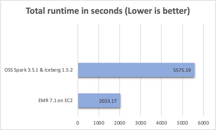
We ran a total of 104 SparkSQL queries in three sequential rounds, and the average runtime of each query across these rounds was taken for comparison. The average runtime for the three rounds on Amazon EMR 7.1 with Iceberg enabled was 0.56 hours, demonstrating a 2.7-fold speed increase compared to open source Spark 3.5.1 and Iceberg 1.5.2. The following figure presents the total runtimes in seconds.

The following table summarizes the metrics.
| Metric |
Amazon EMR 7.1 on EC2 |
Open Source Spark 3.5.1 and Iceberg 1.5.2 |
| Average runtime in seconds |
2033.17 |
5575.19 |
| Geometric mean over queries in seconds |
10.13153 |
20.34651 |
| Cost* |
$7.23 |
$16.09 |
*Detailed cost estimates are discussed later in this post.
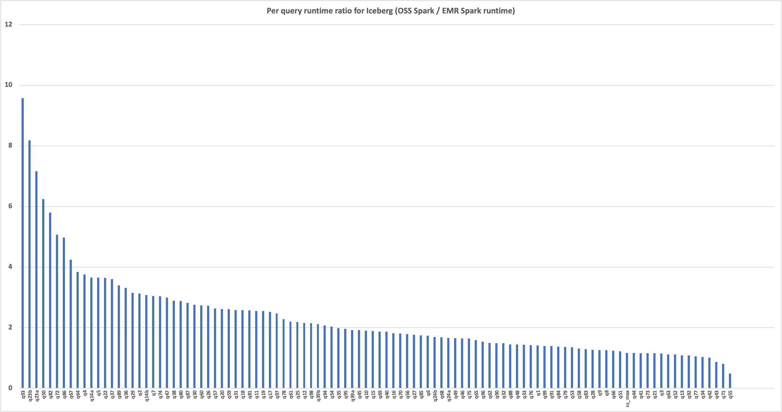
The following chart demonstrates the per-query performance improvement of Amazon EMR 7.1 relative to open source Spark 3.5.1 and Iceberg 1.5.2. The extent of the speedup varies from one query to another, ranging from 9.6 times faster for q93 to 1.04 times faster for q34, with Amazon EMR outperforming the open source Spark with Iceberg tables. The horizontal axis arranges the TPC-DS 3 TB benchmark queries in descending order based on the performance improvement seen with Amazon EMR, and the vertical axis depicts the magnitude of this speedup in seconds.

Cost comparison
Our benchmark provides the total runtime and geometric mean data to assess the performance of Spark and Iceberg in a complex, real-world decision support scenario. For additional insights, we also examine the cost aspect. We calculate cost estimates using formulas that account for EC2 On-Demand instances, Amazon Elastic Block Store (Amazon EBS), and Amazon EMR expenses.
- Amazon EC2 cost (includes SSD cost) = number of instances * r5d.4xlarge hourly rate * job runtime in hours
- 4xlarge hourly rate = $1.152 per hour
- Root Amazon EBS cost = number of instances * Amazon EBS per GB-hourly rate * root EBS volume size * job runtime in hours
- Amazon EMR cost = number of instances * r5d.4xlarge Amazon EMR cost * job runtime in hours
- 4xlarge Amazon EMR cost = $0.27 per hour
- Total cost = Amazon EC2 cost + root Amazon EBS cost + Amazon EMR cost
The calculations reveal that the Amazon EMR 7.1 benchmark yields a 2.2-fold cost efficiency improvement over open source Spark 3.5.1 and Iceberg 1.5.2 in running the benchmark job.
| Metric |
Amazon EMR 7.1 |
Open Source Spark 3.5.1 and Iceberg 1.5.2 |
| Runtime in hours |
0.564 |
1.548 |
| Number of EC2 instances |
9 |
9 |
| Amazon EBS Size |
20gb |
20gb |
| Amazon EC2 cost |
$5.85 |
$16.05 |
| Amazon EBS cost |
$0.01 |
$0.04 |
| Amazon EMR cost |
$1.37 |
$0 |
| Total cost |
$7.23 |
$16.09 |
| Cost savings |
Amazon EMR 7.1 is 2.2 times better |
Baseline |
In addition to the time-based metrics discussed so far, data from Spark event logs shows that Amazon EMR 7.1 scanned approximately 3.4 times less data from Amazon S3 and 4.1 times fewer records than the open source version in the TPC-DS 3 TB benchmark. This reduction in Amazon S3 data scanning contributes directly to cost savings for Amazon EMR workloads.
Run open source Spark benchmarks on Iceberg tables
We used separate EC2 clusters, each equipped with nine r5d.4xlarge instances, for testing both open source Spark 3.5.1 and Iceberg 1.5.2 and Amazon EMR 7.1. The primary node was equipped with 16 vCPU and 128 GB of memory, and the eight worker nodes together had 128 vCPU and 1024 GB of memory. We conducted tests using the Amazon EMR default settings to showcase the typical user experience and minimally adjusted the settings of Spark and Iceberg to maintain a balanced comparison.
The following table summarizes the Amazon EC2 configurations for the primary node and eight worker nodes of type r5d.4xlarge.
| EC2 Instance |
vCPU |
Memory (GiB) |
Instance Storage (GB) |
EBS Root Volume (GB) |
| r5d.4xlarge |
16 |
128 |
2 x 300 NVMe SSD |
20 GB |
Prerequisites
The following prerequisites are required to run the benchmarking:
- Using the instructions in the emr-spark-benchmark GitHub repo, set up the TPC-DS source data in your S3 bucket and on your local computer.
- Build the benchmark application following the steps provided in Steps to build spark-benchmark-assembly application and copy the benchmark application to your S3 bucket. Alternatively, copy spark-benchmark-assembly-3.5.1.jar to your S3 bucket.
- Create Iceberg tables from the TPC-DS source data. Follow the instructions on GitHub to create Iceberg tables using the Hadoop catalog. For example, the following code uses an EMR 7.1 cluster with Iceberg enabled to create the tables:
aws emr add-steps --cluster-id <cluster-id> --steps Type=Spark,Name="Create Iceberg Tables",
Args=[--class,com.amazonaws.eks.tpcds.CreateIcebergTables,
--conf,spark.sql.extensions=org.apache.iceberg.spark.extensions.IcebergSparkSessionExtensions,
--conf,spark.sql.catalog.hadoop_catalog=org.apache.iceberg.spark.SparkCatalog,
--conf,spark.sql.catalog.hadoop_catalog.type=hadoop,
--conf,spark.sql.catalog.hadoop_catalog.warehouse=s3://<bucket>/<warehouse_path>/,
--conf,spark.sql.catalog.hadoop_catalog.io-impl=org.apache.iceberg.aws.s3.S3FileIO,
s3://<bucket>/<jar_location>/spark-benchmark-assembly-3.5.1.jar,
s3://blogpost-sparkoneks-us-east-1/blog/BLOG_TPCDS-TEST-3T-partitioned/,
/home/hadoop/tpcds-kit/tools,parquet,3000,true,<database_name>,true,true],ActionOnFailure=CONTINUE
--region <AWS region>
Note the Hadoop catalog warehouse location and database name from the preceding step. We use the same tables to run benchmarks with Amazon EMR 7.1 and open source Spark and Iceberg.
This benchmark application is built from the branch tpcds-v2.13_iceberg. If you’re building a new benchmark application, switch to the correct branch after downloading the source code from the GitHub repo.
Create and configure a YARN cluster on Amazon EC2
To compare Iceberg performance between Amazon EMR on Amazon EC2 and open source Spark on Amazon EC2, follow the instructions in the emr-spark-benchmark GitHub repo to create an open source Spark cluster on Amazon EC2 using Flintrock with eight worker nodes.
Based on the cluster selection for this test, the following configurations are used:
Run the TPC-DS benchmark with Apache Spark 3.5.1 and Iceberg 1.5.2
Complete the following steps to run the TPC-DS benchmark:
- Log in to the open source cluster primary using
flintrock login $CLUSTER_NAME.
- Submit your Spark job:
- Choose the correct Iceberg catalog warehouse location and database that has the created Iceberg tables.
- The results are created in
s3://<YOUR_S3_BUCKET>/benchmark_run.
- You can track progress in
/media/ephemeral0/spark_run.log.
spark-submit \
--master yarn \
--deploy-mode client \
--class com.amazonaws.eks.tpcds.BenchmarkSQL \
--conf spark.driver.cores=4 \
--conf spark.driver.memory=10g \
--conf spark.executor.cores=16 \
--conf spark.executor.memory=100g \
--conf spark.executor.instances=8 \
--conf spark.network.timeout=2000 \
--conf spark.executor.heartbeatInterval=300s \
--conf spark.dynamicAllocation.enabled=false \
--conf spark.shuffle.service.enabled=false \
--conf spark.hadoop.fs.s3a.aws.credentials.provider=com.amazonaws.auth.InstanceProfileCredentialsProvider \
--conf spark.hadoop.fs.s3.impl=org.apache.hadoop.fs.s3a.S3AFileSystem \
--conf spark.jars.packages=org.apache.hadoop:hadoop-aws:3.3.4,org.apache.iceberg:iceberg-spark-runtime-3.5_2.12:1.5.2,org.apache.iceberg:iceberg-aws-bundle:1.5.2 \
--conf spark.sql.extensions=org.apache.iceberg.spark.extensions.IcebergSparkSessionExtensions   \
--conf spark.sql.catalog.local=org.apache.iceberg.spark.SparkCatalog    \
--conf spark.sql.catalog.local.type=hadoop  \
--conf spark.sql.catalog.local.warehouse=s3a://<YOUR_S3_BUCKET>/<warehouse_path>/ \
--conf spark.sql.defaultCatalog=local   \
--conf spark.sql.catalog.local.io-impl=org.apache.iceberg.aws.s3.S3FileIO   \
spark-benchmark-assembly-3.5.1.jar   \
s3://<YOUR_S3_BUCKET>/benchmark_run 3000 1 false  \
q1-v2.13,q10-v2.13,q11-v2.13,q12-v2.13,q13-v2.13,q14a-v2.13,q14b-v2.13,q15-v2.13,q16-v2.13,\
q17-v2.13,q18-v2.13,q19-v2.13,q2-v2.13,q20-v2.13,q21-v2.13,q22-v2.13,q23a-v2.13,q23b-v2.13,\
q24a-v2.13,q24b-v2.13,q25-v2.13,q26-v2.13,q27-v2.13,q28-v2.13,q29-v2.13,q3-v2.13,q30-v2.13,\
q31-v2.13,q32-v2.13,q33-v2.13,q34-v2.13,q35-v2.13,q36-v2.13,q37-v2.13,q38-v2.13,q39a-v2.13,\
q39b-v2.13,q4-v2.13,q40-v2.13,q41-v2.13,q42-v2.13,q43-v2.13,q44-v2.13,q45-v2.13,q46-v2.13,\
q47-v2.13,q48-v2.13,q49-v2.13,q5-v2.13,q50-v2.13,q51-v2.13,q52-v2.13,q53-v2.13,q54-v2.13,\
q55-v2.13,q56-v2.13,q57-v2.13,q58-v2.13,q59-v2.13,q6-v2.13,q60-v2.13,q61-v2.13,q62-v2.13,\
q63-v2.13,q64-v2.13,q65-v2.13,q66-v2.13,q67-v2.13,q68-v2.13,q69-v2.13,q7-v2.13,q70-v2.13,\
q71-v2.13,q72-v2.13,q73-v2.13,q74-v2.13,q75-v2.13,q76-v2.13,q77-v2.13,q78-v2.13,q79-v2.13,\
q8-v2.13,q80-v2.13,q81-v2.13,q82-v2.13,q83-v2.13,q84-v2.13,q85-v2.13,q86-v2.13,q87-v2.13,\
q88-v2.13,q89-v2.13,q9-v2.13,q90-v2.13,q91-v2.13,q92-v2.13,q93-v2.13,q94-v2.13,q95-v2.13,\
q96-v2.13,q97-v2.13,q98-v2.13,q99-v2.13,ss_max-v2.13    \
true <database> > /media/ephemeral0/spark_run.log 2>&1 &!
Summarize the results
After the Spark job finishes, retrieve the test result file from the output S3 bucket at s3://<YOUR_S3_BUCKET>/benchmark_run/timestamp=xxxx/summary.csv/xxx.csv. This can be done either through the Amazon S3 console by navigating to the specified bucket location or by using the Amazon Command Line Interface (AWS CLI). The Spark benchmark application organizes the data by creating a timestamp folder and placing a summary file within a folder labeled summary.csv. The output CSV files contain four columns without headers:
- Query name
- Median time
- Minimum time
- Maximum time
With the data from three separate test runs with one iteration each time, we can calculate the average and geometric mean of the benchmark runtimes.
Run the TPC-DS benchmark with the EMR runtime for Spark
Most of the instructions are similar to Steps to run Spark Benchmarking with a few Iceberg-specific details.
Prerequisites
Complete the following prerequisite steps:
- Run
aws configure to configure the AWS CLI shell to point to the benchmarking AWS account. Refer to Configure the AWS CLI for instructions.
- Upload the benchmark application JAR file to Amazon S3.
Deploy the EMR cluster and run the benchmark job
Complete the following steps to run the benchmark job:
- Use the AWS CLI command as shown in Deploy EMR on EC2 Cluster and run benchmark job to spin up an EMR on EC2 cluster. Make sure to enable Iceberg. See Create an Iceberg cluster for more details. Choose the correct Amazon EMR version, root volume size, and same resource configuration as the open source Flintrock setup. Refer to create-cluster for a detailed description of the AWS CLI options.
- Store the cluster ID from the response. We need this for the next step.
- Submit the benchmark job in Amazon EMR using
add-steps from the AWS CLI:
- Replace <cluster ID> with the cluster ID from Step 2.
- The benchmark application is at
s3://<your-bucket>/spark-benchmark-assembly-3.5.1.jar.
- Choose the correct Iceberg catalog warehouse location and database that has the created Iceberg tables. This should be the same as the one used for the open source TPC-DS benchmark run.
- The results will be in
s3://<your-bucket>/benchmark_run.
aws emr add-steps   --cluster-id <cluster-id>
--steps Type=Spark,Name="SPARK Iceberg EMR TPCDS Benchmark Job",
Args=[--class,com.amazonaws.eks.tpcds.BenchmarkSQL,
--conf,spark.driver.cores=4,
--conf,spark.driver.memory=10g,
--conf,spark.executor.cores=16,
--conf,spark.executor.memory=100g,
--conf,spark.executor.instances=8,
--conf,spark.network.timeout=2000,
--conf,spark.executor.heartbeatInterval=300s,
--conf,spark.dynamicAllocation.enabled=false,
--conf,spark.shuffle.service.enabled=false,
--conf,spark.sql.iceberg.data-prefetch.enabled=true,
--conf,spark.sql.extensions=org.apache.iceberg.spark.extensions.IcebergSparkSessionExtensions,
--conf,spark.sql.catalog.local=org.apache.iceberg.spark.SparkCatalog,
--conf,spark.sql.catalog.local.type=hadoop,
--conf,spark.sql.catalog.local.warehouse=s3://<your-bucket>/<warehouse-path>,
--conf,spark.sql.defaultCatalog=local,
--conf,spark.sql.catalog.local.io-impl=org.apache.iceberg.aws.s3.S3FileIO,
s3://<your-bucket>/spark-benchmark-assembly-3.5.1.jar,
s3://<your-bucket>/benchmark_run,3000,1,false,
'q1-v2.13\,q10-v2.13\,q11-v2.13\,q12-v2.13\,q13-v2.13\,q14a-v2.13\,
q14b-v2.13\,q15-v2.13\,q16-v2.13\,q17-v2.13\,q18-v2.13\,q19-v2.13\,
q2-v2.13\,q20-v2.13\,q21-v2.13\,q22-v2.13\,q23a-v2.13\,q23b-v2.13\,
q24a-v2.13\,q24b-v2.13\,q25-v2.13\,q26-v2.13\,q27-v2.13\,q28-v2.13\,
q29-v2.13\,q3-v2.13\,q30-v2.13\,q31-v2.13\,q32-v2.13\,q33-v2.13\,
q34-v2.13\,q35-v2.13\,q36-v2.13\,q37-v2.13\,q38-v2.13\,q39a-v2.13\,
q39b-v2.13\,q4-v2.13\,q40-v2.13\,q41-v2.13\,q42-v2.13\,q43-v2.13\,
q44-v2.13\,q45-v2.13\,q46-v2.13\,q47-v2.13\,q48-v2.13\,q49-v2.13\,
q5-v2.13\,q50-v2.13\,q51-v2.13\,q52-v2.13\,q53-v2.13\,q54-v2.13\,
q55-v2.13\,q56-v2.13\,q57-v2.13\,q58-v2.13\,q59-v2.13\,q6-v2.13\,
q60-v2.13\,q61-v2.13\,q62-v2.13\,q63-v2.13\,q64-v2.13\,q65-v2.13\,
q66-v2.13\,q67-v2.13\,q68-v2.13\,q69-v2.13\,q7-v2.13\,q70-v2.13\,
q71-v2.13\,q72-v2.13\,q73-v2.13\,q74-v2.13\,q75-v2.13\,q76-v2.13\,
q77-v2.13\,q78-v2.13\,q79-v2.13\,q8-v2.13\,q80-v2.13\,q81-v2.13\,
q82-v2.13\,q83-v2.13\,q84-v2.13\,q85-v2.13\,q86-v2.13\,q87-v2.13\,
q88-v2.13\,q89-v2.13\,q9-v2.13\,q90-v2.13\,q91-v2.13\,q92-v2.13\,
q93-v2.13\,q94-v2.13\,q95-v2.13\,q96-v2.13\,q97-v2.13\,q98-v2.13\,
q99-v2.13\,ss_max-v2.13',true,<database>],ActionOnFailure=CONTINUE
--region <aws-region>
Summarize the results
After the step is complete, you can see the summarized benchmark result at s3://<YOUR_S3_BUCKET>/benchmark_run/timestamp=xxxx/summary.csv/xxx.csv in the same way as the previous run and compute the average and geometric mean of the query runtimes.
Clean up
To prevent any future charges, delete the resources you created by following the instructions provided in the Cleanup section of the GitHub repository.
Summary
Amazon EMR is consistently enhancing the EMR runtime for Spark when used with Iceberg tables, achieving a performance that is 2.7 times faster than open source Spark 3.5.1 and Iceberg 1.5.2 on TPC-DS 3 TB, v2.13. We encourage you to keep up to date with the latest Amazon EMR releases to fully benefit from ongoing performance improvements.
To stay informed, subscribe to the AWS Big Data Blog’s RSS feed, where you can find updates on the EMR runtime for Spark and Iceberg, as well as tips on configuration best practices and tuning recommendations.
About the authors
 Hari Kishore Chaparala is a software development engineer for Amazon EMR at Amazon Web Services.
Udit Mehrotra is an Engineering Manager for EMR at Amazon Web Services.