Post Syndicated from George Komninos original https://aws.amazon.com/blogs/big-data/design-and-build-a-data-vault-model-in-amazon-redshift-from-a-transactional-database/
Building a highly performant data model for an enterprise data warehouse (EDW) has historically involved significant design, development, administration, and operational effort. Furthermore, the data model must be agile and adaptable to change while handling the largest volumes of data efficiently.
Data Vault is a methodology for delivering project design and implementation to accelerate the build of data warehouse projects. Within the overall methodology, the Data Vault 2.0 data modeling standards are popular and widely used within the industry because they emphasize the business keys and their associations within the delivery of business processes. Data Vault facilitates the rapid build of data models via the following:
- Pattern-based entities each with a well-defined purpose
- Data silos are removed because data is represented in source system independent structures
- Data can be loaded in parallel with minimum dependencies
- Historized data is stored at its lowest level of granularity
- Flexible business rules can be applied independently of the loading of the data
- New data sources can be added with no impact on the existing model.
We always recommend working backwards from the business requirements to choose the most suitable data modelling pattern to use; there are times where Data Vault will not be the best choice for your enterprise data warehouse and another modelling pattern will be more suitable.
In this post, we demonstrate how to implement a Data Vault model in Amazon Redshift and query it efficiently by using the latest Amazon Redshift features, such as separation of compute from storage, seamless data sharing, automatic table optimizations, and materialized views.
Data Vault data modeling overview
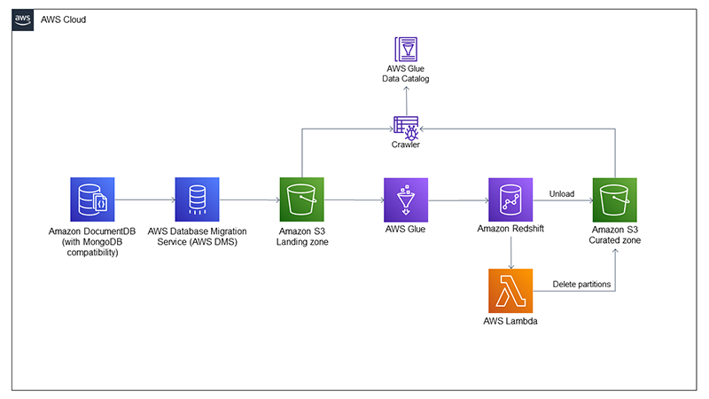
A data warehouse platform built using Data Vault typically has the following architecture:

The architecture consists of four layers:
- Staging – Contains a copy of the latest changes to data from the source systems. This layer doesn’t hold history and, during its population, you can apply several transformations to the staged data, including data type changes or resizing, character set conversion, and the addition of meta-data columns to support later processing.
- Raw Data Vault – Holds the historized copy of all of the data from multiple source systems. No filters or business transformations have occurred at this point except for storing the data in source-system independent targets.
- Business Data Vault – An optional delivery, but is very often built. It contains business calculations and de-normalizations with the sole purpose of improving the speed and simplicity of access within the consumption layer, which is called the Information Mart layer.
- Information Mart Layer – Where data is most commonly accessed by consumers, for example reporting dashboards or extracts. You can build multiple marts from the one Data Vault Integration Layer, and the most common data modeling choice for these marts is Star/Kimball schemas.
Convert a Third Normal Form transactional schema to a Data Vault schema
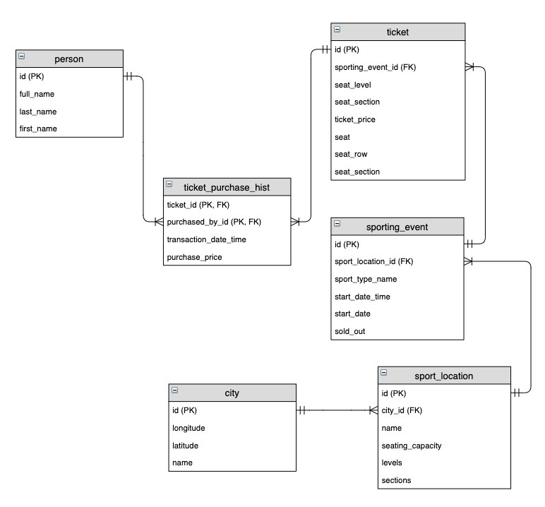
The following entity relationship diagram is a standard implementation of a transactional model that a sports ticket selling service could use:

The main entities within the schema are sporting events, customers, and tickets. A customer is a person, and a person can purchase one or multiple tickets for a sporting event. This business event is captured by the Ticket Purchase History intersection entity above. Finally, a sporting event has many tickets available to purchase and is staged within a single city.
To convert this source model to a Data Vault model, we start to identify the business keys, their descriptive attributes, and the business transactions. The three main entity types in the Raw Data Vault model are as follows:
- Hubs – A collection of Business Keys discovered for each business entity.
- Links – Business transactions within the process being modelled. This is always between two or more business keys (hubs) and recorded at a point in time.
- Satellites – Historized reference data about either the business key (Hub) or business transaction (link).
The following example solution represents some of the sporting event entities when converted into the preceeding Raw Data Vault objects.
Hub entities
The hub is the definitive list of business keys loaded into the Raw Data Vault layer from all of the source systems. A business key is used to uniquely identify a business entity and is never duplicated. In our example, the source system has assigned a surrogate key field called Id to represent the Business Key, so this is stored in a column on the Hub called sport_event_id. Some common additional columns on hubs include the Load DateTimeStamp which records the date and time the business key was first discovered, and the Record Source which records the name of the source system where this business key was first loaded. Although, you don’t have to create a surrogate type (hash or sequence) for the primary key column, it is very common in Data Vault to hash the business key, so our example does this. Amazon Redshift supports multiple cryptographic hash functions like MD5, FNV, SHA1, and SHA2, which you can choose to generate your primary key column. See the following code :
create table raw_data_vault.hub_sport_event
(
  sport_event_pk  varchar(32) not null
 ,sport_event_id  integer     not null
 ,load_dts        timestamp   not null
 ,record_source   varchar(10) not null
);
Note the following:
- The preceeding code assumes the MD5 hashing algorithm is used. If using FNV_HASH, the datatype will be Bigint.
- The Id column is the business key from the source feed. It’s passed into the hashing function for the
_PK column.
- In our example, there is only a single value for the business key. If a compound key is required, then more than one column can be added.
- Load_DTS is populated via the staging schema or extract, transform, and load (ETL) code.
- Record_Source is populated via the staging schema or ETL code.
Link entities
The link object is the occurrence of two or more business keys undertaking a business transaction, for example purchasing a ticket for a sporting event. Each of the business keys is mastered in their respective hubs, and a primary key is generated for the link comprising all of the business keys (typically separated by a delimiter field like ‘^’). As with hubs, some common additional columns are added to links, including the Load DateTimeStamp which records the date and time the transaction was first discovered, and the Record Source which records the name of the source system where this transaction was first loaded. See the following code:
create table raw_data_vault.lnk_ticket_sport_event
(
  ticket_sport_event_pk varchar(32)  not null
 ,ticket_fk             varchar(32)  not null
 ,sport_event_fk        varchar(32)  not null
 ,load_dts              timestamp    not null
 ,record_source         varchar(10)  not null
);
Note the following:
- The code assumes that the MD5 hashing algorithm is used. The
_PK column is hashed values of concatenated ticket and sporting event business keys from the source data feed, for example MD5(ticket_id||'^'||sporting_event_id)
- The two
_FK columns are foreign keys linked to the primary key of the respective hubs.
- Load_DTS is populated via the staging schema or ETL code.
- Record_Source is populated via the staging schema or ETL code.
Satellite entities
The history of data about the hub or link is stored in the satellite object. The Load DateTimeStamp is part of the compound key of the satellite along with the primary key of either the hub or link because data can change over time. There are choices within the Data Vault standards for how to store satellite data from multiple sources. A common approach is to append the name of the feed to the satellite name. This lets a single hub contain reference data from more than one source system, and for new sources to be added without impact to the existing design. See the following code:
create table raw_data_vault.sat_sport_event
(
  sport_event_pk    varchar(32) not null
 ,load_dts          timestamp   not null
 ,sport_type_name   varchar(50)
 ,start_datetime    timestamp
 ,sold_out          boolean
 ,record_source     varchar(10) not null
 ,hash_diff         varchar(32) not null
);
Note the following:
- The
sport_event_pk value is inherited from the hub.
- The compound key is the
sport_event_pk and load_dts columns. This allows history to be maintained.
- The business attributes are typically optional.
Load_DTS is populated via the staging schema or ETL code.- Record_Source is populated via the staging schema or ETL code.
- Hash_Diff is a Data Vault technique to simplify the identification of data changes within satellites. The business attribute values are concatenated and hashed with your algorithm of choice. Then, during the ETL processing, only the two hash values (one on the source record and one on the latest dated satellite record) should be compared.
Converted Data Vault Model
If we take the preceding three Data Vault entity types above, we can convert the source data model into a Data Vault data model as follows:

The Business Data Vault contains business-centric calculations and performance de-normalizations that are read by the Information Marts. Some of the object types that are created in the Business Vault layer include the following:
- PIT (point in time) tables – You can store data in more than one satellite for a single hub, each with a different
Load DateTimeStamp depending on when the data was loaded. A PIT table simplifies access to all of this data by creating a table or materialized view to present a single row with all of the relevant data to hand. The compound key of a PIT table is the primary key from the hub, plus a snapshot date or snapshot date and time for the frequency of the population. Once a day is the most popular, but equally the frequency could be every 15 minutes or once a month.
- Bridge tables – Similar to PIT tables, bridge tables take the data from more than one link or link satellite and again de-normalize into a single row. This single row view makes accessing complex datasets over multiple tables from the Raw Data Vault much more straightforward and performant. Like a PIT table, the bridge table can be either a table or materialized view.
- KPI tables – The pre-computed business rules calculate KPIs and store them in dedicated tables.
- Type 2 tables –You can apply additional processing in the Business Data Vault to calculate Type 2 like time periods because the data in the Raw Data Vault follows an insert only pattern.
The architecture of Amazon Redshift allows flexibility in the design of the Data Vault platform by using the capabilities of the Amazon Redshift RA3 instance type to separate the compute resources from the data storage layer and the seamless ability to share data between different Amazon Redshift clusters. This flexibility allows highly performant and cost-effective Data Vault platforms to be built. For example, the Staging and Raw Data Vault Layers are populated 24-hours-a-day in micro batches by one Amazon Redshift cluster, the Business Data Vault layer can be built one-time-a-day and paused to save costs when completed, and any number of consumer Amazon Redshift clusters can access the results. Depending on the processing complexity of each layer, Amazon Redshift supports independently scaling the compute capacity required at each stage.

All of the underlying tables in Raw Data Vault can be loaded simultaneously. This makes great use of the massively parallel processing architecture in Amazon Redshift. For our business model, it makes sense to create a Business Data Vault layer, which can be read by an Information Mart to perform dimensional analysis on ticket sales. It can give us insights on the top home teams in fan attendance and how that correlates with specific sport locations or cities. Running these queries involves joining multiple tables. It’s important to design an optimal Business Data Vault layer to avoid excessive joins for deriving these insights.
For example, to get the number of tickets per city for June 2021, the SQL looks like the following code:
SELECT name,count(lpt.ticket_fk) as tickets_sold
FROM lnk_person_ticket lpt
  JOIN lnk_ticket_sport_event ltse on lpt.ticket_fk = ltse.ticket_fk
  JOIN lnk_sport_event_location lsel on ltse.sport_event_fk = lsel.sport_event_fk
  JOIN lnk_location_city llc on lsel.location_fk = llc.location_fk
  JOIN sat_city sc on llc.city_fk = sc.city_pk
  JOIN sat_sport_event sse on lsel.sport_event_fk = sse.sport_event_pk
Where start_date between '2021-06-05' and '2021-06-15' group by 1;
We can use the EXPLAIN command for the preceding query to get the Amazon Redshift query plan. The following plan shows that the specified joins require broadcasting data across nodes, since the join conditions are on different keys. This makes the query computationally expensive:
dev=# explain SELECT
  name, count(lpt.ticket_fk) as tickets_sold FROM lnk_person_ticket lpt
  JOIN lnk_ticket_sport_event ltse on lpt.ticket_fk = ltse.ticket_fk
  JOIN lnk_sport_event_location lsel on ltse.sport_event_fk = lsel.sport_event_fk
  JOIN lnk_location_city llc on lsel.location_fk = llc.location_fk
  JOIN sat_city sc on llc.city_fk = sc.city_pk
  JOIN sat_sport_event sse on lsel.sport_event_fk = sse.sport_event_pk
where
  start_date between ‘2021-06-05’
  and ‘2021-06-15’
GROUP BY
  1;
                            QUERY PLAN
----------------------------------------------------------------------
 XN HashAggregate  (cost=96331086541.29..96331086564.36 rows=9226 width=49)
   ->  XN Hash Join DS_BCAST_INNER  (cost=166693605.84..96331086495.16 rows=9226 width=49)
         Hash Cond: ((“outer”.ticket_fk)::text = (“inner”.ticket_fk)::text)
         ->  XN Hash Join DS_BCAST_INNER  (cost=166690878.95..344629685.90 rows=621783 width=49)
               Hash Cond: ((“outer”.sport_event_fk)::text = (“inner”.sport_event_fk)::text)
               ->  XN Seq Scan on lnk_ticket_sport_event ltse  (cost=0.00..147804.35 rows=14780435 width=72)
               ->  XN Hash  (cost=166690878.49..166690878.49 rows=185 width=85)
                     ->  XN Hash Join DS_BCAST_INNER  (cost=49690773.08..166690878.49 rows=185 width=85)
                           Hash Cond: ((“outer”.location_fk)::text = (“inner”.location_fk)::text)
                           ->  XN Hash Join DS_BCAST_INNER  (cost=65.61..79200165.14 rows=179 width=108)
                                 Hash Cond: ((“outer”.sport_event_fk)::text = (“inner”.sport_event_pk)::text)
                                 ->  XN Seq Scan on lnk_sport_event_location lsel  (cost=0.00..43.44 rows=4344 width=72)
                                 ->  XN Hash  (cost=65.16..65.16 rows=180 width=36)
                                       ->  XN Seq Scan on sat_sport_event sse  (cost=0.00..65.16 rows=180 width=36)
                                             Filter: ((start_date <= ‘2021-06-15’::date) AND (start_date >= ‘2021-06-05’::date))
                           ->  XN Hash  (cost=49690707.31..49690707.31 rows=63 width=49)
                                 ->  XN Hash Join DS_BCAST_INNER  (cost=0.78..49690707.31 rows=63 width=49)
                                       Hash Cond: ((“outer”.city_pk)::text = (“inner”.city_fk)::text)
                                       ->  XN Seq Scan on sat_city sc  (cost=0.00..27909.51 rows=2790951 width=49)
                                       ->  XN Hash  (cost=0.62..0.62 rows=62 width=72)
                                             ->  XN Seq Scan on lnk_location_city llc  (cost=0.00..0.62 rows=62 width=72)
         ->  XN Hash  (cost=2181.51..2181.51 rows=218151 width=36)
               ->  XN Seq Scan on lnk_person_ticket lpt  (cost=0.00..2181.51 rows=218151 width=36)
(23 rows)
Let’s discuss the latest Amazon Redshift features that help optimize the performance of these queries on top of a Business Data Vault model.
Use Amazon Redshift features to query the Data Vault
Automatic table optimization
Traditionally, to optimize joins in Amazon Redshift, it’s recommended to use distribution keys and styles to co-locate data in the same nodes, as based on common join predicates. The Raw Data Vault layer has a very well-defined pattern, which is ideal for determining the distribution keys. However, the broad range of SQL queries applicable to the Business Data Vault makes it hard to predict your consumption pattern that would drive your distribution strategy.
Automatic table optimization lets you get the fastest performance quickly without needing to invest time to manually tune and implement table optimizations. Automatic table optimization continuously observes how queries interact with tables, and it uses machine learning (ML) to select the best sort and distribution keys to optimize performance for the cluster’s workload. If Amazon Redshift determines that applying a key will improve cluster performance, then tables are automatically altered within hours without requiring administrator intervention.
Automatic Table Optimization provided following recommendations for the above query to get the number of tickets per city for June 2021. The recommendations suggest modifying the distribution style and sort keys for tables involved in these queries.
dev=# select * from svv_alter_table_recommendations;
   type    | database | table_id | group_id |                                           ddl                                           | auto_eligible
-----------+----------+----------+----------+-----------------------------------------------------------------------------------------+---------------
 diststyle | dev      |   127372 |        0 | ALTER TABLE “public”.“lnk_person_ticket” ALTER DISTSTYLE KEY DISTKEY “ticket_fk”        | f
 sortkey   | dev      |   127421 |       -1 | ALTER TABLE “public”.“lnk_ticket_sport_event” ALTER COMPOUND SORTKEY (“sport_event_fk”) | f
 diststyle | dev      |   127421 |        0 | ALTER TABLE “public”.“lnk_ticket_sport_event” ALTER DISTSTYLE KEY DISTKEY “ticket_fk”   | f
 sortkey   | dev      |   145032 |       -1 | ALTER TABLE “public”.“sat_city” ALTER COMPOUND SORTKEY (“city_pk”)                      | f
After the recommended distribution keys and sort keys were applied by Automatic Table Optimization, the explain plan shows “DS_DIST_NONE” and no data redistribution was required anymore for this query. The data required for the joins was co-located across Amazon Redshift nodes.
QUERY PLAN
----------------------------------------------------------------------
 XN HashAggregate  (cost=344646541.29..344646564.36 rows=9226 width=49)
   ->  XN Hash Join DS_DIST_NONE  (cost=166693605.84..344646495.16 rows=9226 width=49)
         Hash Cond: ((“outer”.ticket_fk)::text = (“inner”.ticket_fk)::text)
         ->  XN Hash Join DS_BCAST_INNER  (cost=166690878.95..344629685.90 rows=621783 width=49)
               Hash Cond: ((“outer”.sport_event_fk)::text = (“inner”.sport_event_fk)::text)
               ->  XN Seq Scan on lnk_ticket_sport_event ltse  (cost=0.00..147804.35 rows=14780435 width=72)
               ->  XN Hash  (cost=166690878.49..166690878.49 rows=185 width=85)
                     ->  XN Hash Join DS_BCAST_INNER  (cost=49690773.08..166690878.49 rows=185 width=85)
                           Hash Cond: ((“outer”.location_fk)::text = (“inner”.location_fk)::text)
                           ->  XN Hash Join DS_BCAST_INNER  (cost=65.61..79200165.14 rows=179 width=108)
                                 Hash Cond: ((“outer”.sport_event_fk)::text = (“inner”.sport_event_pk)::text)
                                 ->  XN Seq Scan on lnk_sport_event_location lsel  (cost=0.00..43.44 rows=4344 width=72)
                                 ->  XN Hash  (cost=65.16..65.16 rows=180 width=36)
                                       ->  XN Seq Scan on sat_sport_event sse  (cost=0.00..65.16 rows=180 width=36)
                                             Filter: ((start_date <= ‘2021-06-15’::date) AND (start_date >= ‘2021-06-05’::date))
                           ->  XN Hash  (cost=49690707.31..49690707.31 rows=63 width=49)
                                 ->  XN Hash Join DS_BCAST_INNER  (cost=0.78..49690707.31 rows=63 width=49)
                                       Hash Cond: ((“outer”.city_pk)::text = (“inner”.city_fk)::text)
                                       ->  XN Seq Scan on sat_city sc  (cost=0.00..27909.51 rows=2790951 width=49)
                                       ->  XN Hash  (cost=0.62..0.62 rows=62 width=72)
                                             ->  XN Seq Scan on lnk_location_city llc  (cost=0.00..0.62 rows=62 width=72)
         ->  XN Hash  (cost=2181.51..2181.51 rows=218151 width=36)
               ->  XN Seq Scan on lnk_person_ticket lpt  (cost=0.00..2181.51 rows=218151 width=36)
(23 rows)
Materialized views in Amazon Redshift
The data analyst responsible for running this analysis benefits significantly by creating a materialized view in the Business Data Vault schema that pre-computes the results of the queries by running the following SQL:
CREATE MATERIALIZED VIEW bridge_city_ticket_aggregation_mv
AUTO REFRESH YES
AS SELECT name, count(lpt.ticket_fk) as tickets_sold
FROM lnk_person_ticket lpt
JOIN lnk_ticket_sport_event ltse on lpt.ticket_fk = ltse.ticket_fk
JOIN lnk_sport_event_location lsel on ltse.sport_event_fk = lsel.sport_event_fk
JOIN lnk_location_city llc on lsel.location_fk = llc.location_fk
JOIN sat_city sc on llc.city_fk = sc.city_pk
GROUP BY 1;
To get the latest satellite values, we must include load_dts in our join. For simplicity, we don’t do that for this post.
You can optimize this query both in terms of code length and complexity to something as simple as the following:
SELECT * FROM bridge_city_ticket_aggregation_mv;
The run plan in this case is as follows:
XN Seq Scan on mv_tbl__bridge_city_ticket_aggregation_mv__0 derived_table1 (cost=0.00..0.36 rows=36 width=524)
More importantly, Amazon Redshift can automatically use the materialized view even if that’s not explicitly stated.
The preceding scenario addresses the needs of a specific analysis because the resulting materialized view is an aggregate. In a more generic scenario, after reviewing our Data Vault ER diagram, you can observe that any query that involves ticket sales analysis per location requires a substantial number of joins, all of which use different join keys. Therefore, any such analysis comes at a significant cost regarding performance. For example, to get the count of tickets sold per city and stadium name, you must run a query like the following:
SELECT sc.name city_name, ssl.name stadium_name, count(lpt.ticket_fk) tickets_sold
FROM lnk_person_ticket lpt
JOIN lnk_ticket_sport_event ltse ON lpt.ticket_fk = ltse.ticket_fk
JOIN lnk_sport_event_location lsel ON ltse.sport_event_fk = lsel.sport_event_fk
JOIN sat_location ssl ON lsel.location_fk = ssl.location_pk
JOIN lnk_location_city llc ON lsel.location_fk = llc.location_fk
JOIN sat_city sc ON llc.city_fk = sc.city_pk
GROUP BY 1, 2;
You can use the EXPLAIN command for the preceding query to get the explain plan and know how expensive such an operation is:
XN HashAggregate  (cost=99574385259.46..99574385829.64 rows=228071 width=68)
  ->  XN Hash Join DS_BCAST_INNER  (cost=127173776.83..99574383548.93 rows=228071 width=68)
        Hash Cond: (("outer".sport_event_fk)::text = ("inner".sport_event_fk)::text)
        ->  XN Hash Join DS_BCAST_INNER  (cost=2726.89..95986925283.91 rows=219289 width=72)
              Hash Cond: (("outer".ticket_fk)::text = ("inner".ticket_fk)::text)
              ->  XN Seq Scan on lnk_ticket_sport_event ltse  (cost=0.00..147804.35 rows=14780435 width=72)
              ->  XN Hash  (cost=2181.51..2181.51 rows=218151 width=36)
                    ->  XN Seq Scan on lnk_person_ticket lpt  (cost=0.00..2181.51 rows=218151 width=36)
        ->  XN Hash  (cost=127171038.56..127171038.56 rows=4553 width=68)
              ->  XN Hash Join DS_BCAST_INNER  (cost=49690708.24..127171038.56 rows=4553 width=68)
                    Hash Cond: (("outer".location_fk)::text = ("inner".location_fk)::text)
                    ->  XN Hash Join DS_BCAST_INNER  (cost=0.78..39680186.12 rows=4416 width=127)
                          Hash Cond: (("outer".location_fk)::text = ("inner".location_pk)::text)
                          ->  XN Seq Scan on lnk_sport_event_location lsel  (cost=0.00..43.44 rows=4344 width=72)
                          ->  XN Hash  (cost=0.62..0.62 rows=62 width=55)
                                ->  XN Seq Scan on sat_location ssl  (cost=0.00..0.62 rows=62 width=55)
                    ->  XN Hash  (cost=49690707.31..49690707.31 rows=63 width=49)
                          ->  XN Hash Join DS_BCAST_INNER  (cost=0.78..49690707.31 rows=63 width=49)
                                Hash Cond: (("outer".city_pk)::text = ("inner".city_fk)::text)
                                ->  XN Seq Scan on sat_city sc  (cost=0.00..27909.51 rows=2790951 width=49)
                                ->  XN Hash  (cost=0.62..0.62 rows=62 width=72)
                                      ->  XN Seq Scan on lnk_location_city llc  (cost=0.00..0.62 rows=62 width=72)
We can identify commonly joined tables, like hub_sport_event, hub_ticket and hub_location, and then boost the performance of queries by creating materialized views that implement these joins ahead of time. For example, we can create a materialized view to join tickets to sport locations:
CREATE MATERIALIZED VIEW bridge_tickets_per_stadium_mv
AUTO REFRESH YES
AS select hsl.hub_sport_location_key location_id, hub_ticket_seq tickets_id , start_date date, "name" stadium_name
from hub_ticket
join lnk_ticket_sport_event ltse on hub_ticket_seq = hub_ticket_key
join hub_sport_event hse on hse.hub_sport_event_key = ltse.hub_sport_event_seq
join sat_sport_event sse on sse.hub_sport_event_key = hse.hub_sport_event_key
join lnk_sport_event_location lsel on hse.hub_sport_event_key = lsel.hub_sport_event_seq
join hub_sport_location hsl on hub_location_seq = hub_sport_location_key
join sat_sport_location ssl on ssl.hub_sport_location_key = hsl.hub_sport_location_key;
If we don’t make any edits to the expensive query that we ran before, then the run plan is as follows:
XN HashAggregate (cost=88052548.77..88064188.37 rows=4655838 width=457)
-> XN Hash Join DS_BCAST_INNER (cost=49690707.47..88017629.99 rows=4655838 width=457)
Hash Cond: (("outer".location_id)::text = ("inner".hub_location_seq)::text)
-> XN Seq Scan on mv_tbl__bridge_tickets_per_stadium_mv__0 derived_table1 (cost=0.00..147804.35 rows=14780435 width=510)
-> XN Hash (cost=49690707.31..49690707.31 rows=63 width=49)
-> XN Hash Join DS_BCAST_INNER (cost=0.78..49690707.31 rows=63 width=49)
Hash Cond: (("outer".hub_city_key)::text = ("inner".hub_city_seq)::text)
-> XN Seq Scan on hub_city hc (cost=0.00..27909.51 rows=2790951 width=49)
-> XN Hash (cost=0.62..0.62 rows=62 width=72)
-> XN Seq Scan on lnk_location_city llc (cost=0.00..0.62 rows=62 width=72)
Amazon Redshift now uses the materialized view for any future queries that involve joining tickets with sports locations. For example, a separate business intelligence (BI) team looking into the dates with the highest ticket sales can run a query like the following:
select start_date date, count(hub_ticket_seq) tickets
from hub_ticket
join lnk_ticket_sport_event ltse on hub_ticket_seq = hub_ticket_key
join hub_sport_event hse on hse.hub_sport_event_key  = ltse.hub_sport_event_seq
join sat_sport_event sse on sse.hub_sport_event_key = hse.hub_sport_event_key
join lnk_sport_event_location lsel on hse.hub_sport_event_key = lsel.hub_sport_event_seq
join hub_sport_location hsl on hub_location_seq = hub_sport_location_key
join sat_sport_location ssl on ssl.hub_sport_location_key = hsl.hub_sport_location_key
group by 1
order by 2 desc
limit 10;
Amazon Redshift can implicitly understand that the query can be optimized by using the materialized view we already created, thereby avoiding joins that involve broadcasting data across nodes. This can be seen from the run plan:
XN Limit (cost=1000000221707.65..1000000221707.68 rows=10 width=40)
-> XN Merge (cost=1000000221707.65..1000000221707.75 rows=39 width=40)
Merge Key: count(derived_table1.tickets_id)
-> XN Network (cost=1000000221707.65..1000000221707.75 rows=39 width=40)
Send to leader
-> XN Sort (cost=1000000221707.65..1000000221707.75 rows=39 width=40)
Sort Key: count(derived_table1.tickets_id)
-> XN HashAggregate (cost=221706.52..221706.62 rows=39 width=40)
-> XN Seq Scan on mv_tbl__bridge_tickets_per_stadium_mv__0 derived_table1 (cost=0.00..147804.35 rows=14780435 width=40)
If we drop the materialized view, then the preceding query results in the following plan:
XN Limit (cost=7509421514303.64..7509421514303.66 rows=10 width=40)
-> XN Merge (cost=7509421514303.64..7509421514303.73 rows=39 width=40)
Merge Key: count(ltse.hub_ticket_seq)
-> XN Network (cost=7509421514303.64..7509421514303.73 rows=39 width=40)
Send to leader
-> XN Sort (cost=7509421514303.64..7509421514303.73 rows=39 width=40)
Sort Key: count(ltse.hub_ticket_seq)
-> XN HashAggregate (cost=6509421514302.51..6509421514302.61 rows=39 width=40)
-> XN Hash Join DS_BCAST_INNER (cost=54745206.40..6509421439263.58 rows=15007786 width=40)
Hash Cond: (("outer".hub_sport_event_seq)::text = ("inner".hub_sport_event_seq)::text)
-> XN Hash Join DS_BCAST_INNER (cost=184864.04..6507391239560.52 rows=14634339 width=148)
Hash Cond: (("outer".hub_ticket_seq)::text = ("inner".hub_ticket_key)::text)
-> XN Hash Join DS_BCAST_INNER (cost=108.60..3997288304.94 rows=14558405 width=148)
Hash Cond: (("outer".hub_sport_event_seq)::text = ("inner".hub_sport_event_key)::text)
-> XN Hash Join DS_BCAST_INNER (cost=54.30..2085599304.09 rows=14669000 width=112)
Hash Cond: (("outer".hub_sport_event_seq)::text = ("inner".hub_sport_event_key)::text)
-> XN Seq Scan on lnk_ticket_sport_event ltse (cost=0.00..147804.35 rows=14780435 width=72)
-> XN Hash (cost=43.44..43.44 rows=4344 width=40)
-> XN Seq Scan on sat_sport_event sse (cost=0.00..43.44 rows=4344 width=40)
-> XN Hash (cost=43.44..43.44 rows=4344 width=36)
-> XN Seq Scan on hub_sport_event hse (cost=0.00..43.44 rows=4344 width=36)
-> XN Hash (cost=147804.35..147804.35 rows=14780435 width=36)
-> XN Seq Scan on hub_ticket (cost=0.00..147804.35 rows=14780435 width=36)
-> XN Hash (cost=54560331.14..54560331.14 rows=4489 width=36)
-> XN Hash Join DS_BCAST_INNER (cost=1.55..54560331.14 rows=4489 width=36)
Hash Cond: (("outer".hub_location_seq)::text = ("inner".hub_sport_location_key)::text)
-> XN Hash Join DS_BCAST_INNER (cost=0.78..27280186.11 rows=4416 width=108)
Hash Cond: (("outer".hub_location_seq)::text = ("inner".hub_sport_location_key)::text)
-> XN Seq Scan on lnk_sport_event_location lsel (cost=0.00..43.44 rows=4344 width=72)
-> XN Hash (cost=0.62..0.62 rows=62 width=36)
-> XN Seq Scan on sat_sport_location ssl (cost=0.00..0.62 rows=62 width=36)
-> XN Hash (cost=0.62..0.62 rows=62 width=36)
-> XN Seq Scan on hub_sport_location hsl (cost=0.00..0.62 rows=62 width=36)
End-users of the data warehouse don’t need to worry about refreshing the data in the materialized views. This is because we enabled automatic materialized view refresh. Future use cases involving new dimensions also benefit from the existence of materialized views.
Prepared statements in the data vault with materialized views in Amazon Redshift
Another type of query that we can run on top of the Business Data Vault schema is prepared statements with bind variables. It’s quite common to see user interfaces integrated with data warehouses, which lets users dynamically change the value of the variable through selection in a choice list or link in a cross-tab. When the variable changes, so do the query condition and the report or dashboard contents. The following query is a prepared statement to get the count of tickets sold per city and stadium name. It takes the stadium name as a variable and provides the number of tickets sold in that stadium.
PREPARE prep_statement (varchar(100))
AS select hc.name city_name, ssl."name" stadium_name, count(hub_ticket_seq) tickets
 from hub_ticket
 join lnk_ticket_sport_event ltse on hub_ticket_seq = hub_ticket_key
 join hub_sport_event hse on hse.hub_sport_event_key = ltse.hub_sport_event_seq
 join sat_sport_event sse on sse.hub_sport_event_key = hse.hub_sport_event_key
 join lnk_sport_event_location lsel on hse.hub_sport_event_key = lsel.hub_sport_event_seq
 join hub_sport_location hsl on hub_location_seq = hub_sport_location_key
 join sat_sport_location ssl on ssl.hub_sport_location_key = hsl.hub_sport_location_key
 join lnk_location_city llc on llc.hub_location_seq = hsl.hub_sport_location_key
 join hub_city hc on llc.hub_city_seq = hc.hub_city_key
 where ssl."name"  = $1
 group by 1, 2;
PREPARE
Let’s run the query to see the city and tickets sold for different stadiums passed as a variable in this prepared statement:
dev=# EXECUTE prep_statement('Lucas Oil Stadium');
  city_name   |   stadium_name    | tickets
--------------+-------------------+---------
 Indianapolis | Lucas Oil Stadium |    8892
(1 row)

dev=# EXECUTE prep_statement('Ford Field');
 city_name | stadium_name | tickets
-----------+--------------+---------
 Detroit   | Ford Field   |   42720
(1 row)
Let’s dive into the explain plan of this prepared statement to understand if Amazon Redshift can implicitly understand that the query can be optimized by using the materialized view bridge_tickets_per_stadium_mv that was created earlier:
XN HashAggregate  (cost=87685290.31..87685914.69 rows=249748 width=66)
->  XN Hash Join DS_BCAST_INNER  (cost=49690707.47..87683417.20 rows=249748 width=66)
Hash Cond: (("outer".location_id)::text = ("inner".hub_location_seq)::text)
->  XN Seq Scan on *mv_tbl__bridge_tickets_per_stadium_mv__0* derived_table1  (cost=0.00..184755.44 rows=242303 width=89)
*Filter: ((stadium_name)::text = ($1)::text)*
->  XN Hash  (cost=49690707.31..49690707.31 rows=63 width=49)
->  XN Hash Join DS_BCAST_INNER  (cost=0.78..49690707.31 rows=63 width=49)
Hash Cond: (("outer".hub_city_key)::text = ("inner".hub_city_seq)::text)
->  XN Seq Scan on hub_city hc  (cost=0.00..27909.51 rows=2790951 width=49)
->  XN Hash  (cost=0.62..0.62 rows=62 width=72)
->  XN Seq Scan on lnk_location_city llc  (cost=0.00..0.62 rows=62 width=72)
As noted in the explain plan, Amazon Redshift could optimize the explain plan of the query to implicitly use the materialized view created earlier, even for prepared statements.
Conclusion
In this post, we’ve demonstrated how to implement Data Vault model in Amazon Redshift, thereby levering the out-of-the-box features. We also discussed how Amazon Redshift’s features, such as seamless data share, automatic table optimization, materialized views, and automatic materialized view refresh can help you build data models that meet high performance requirements.
About the Authors
 George Komninos is a solutions architect for the AWS Data Lab. He helps customers convert their ideas to a production-ready data products. Before AWS, he spent three years at Alexa Information as a data engineer. Outside of work, George is a football fan and supports the greatest team in the world, Olympiacos Piraeus.
 Devika Singh is a Senior Solutions Architect at Amazon Web Services. Devika helps customers architect and build database and data analytics solutions to accelerate their path to production as part of the AWS Data Lab. She has expertise in database and data warehouse migrations to AWS, helping customers improve the value of their solutions with AWS.
 Simon Dimaline has specialized in data warehousing and data modeling for more than 20 years. He currently works for the Data & Analytics practice within AWS Professional Services accelerating customers’ adoption of AWS analytics services.


 George Komninos is a solutions architect for the AWS Data Lab. He helps customers convert their ideas to a production-ready data product. Before AWS, he spent three years at Alexa Information domain as a data engineer. Outside of work, George is a football fan and supports the greatest team in the world, Olympiacos Piraeus.


 George Komninos is a Data Lab Solutions Architect at AWS. He helps customers convert their ideas to a production-ready data product. Before AWS, he spent 3 years at Alexa Information domain as a data engineer. Outside of work, George is a football fan and supports the greatest team in the world, Olympiacos Piraeus.
 Sakti Mishra is a Data Lab Solutions Architect at AWS. He helps customers architect data analytics solutions, which gives them an accelerated path towards modernization initiatives. Outside of work, Sakti enjoys learning new technologies, watching movies, and travel.