Tag Archives: AWS Data Lab

How Zoom implemented streaming log ingestion and efficient GDPR deletes using Apache Hudi on Amazon EMR

Post Syndicated from Sekar Srinivasan original https://aws.amazon.com/blogs/big-data/how-zoom-implemented-streaming-log-ingestion-and-efficient-gdpr-deletes-using-apache-hudi-on-amazon-emr/

In today’s digital age, logging is a critical aspect of application development and management, but efficiently managing logs while complying with data protection regulations can be a significant challenge. Zoom, in collaboration with the AWS Data Lab team, developed an innovative architecture to overcome these challenges and streamline their logging and record deletion processes. In this post, we explore the architecture and the benefits it provides for Zoom and its users.

Application log challenges: Data management and compliance

Application logs are an essential component of any application; they provide valuable information about the usage and performance of the system. These logs are used for a variety of purposes, such as debugging, auditing, performance monitoring, business intelligence, system maintenance, and security. However, although these application logs are necessary for maintaining and improving the application, they also pose an interesting challenge. These application logs may contain personally identifiable data, such as user names, email addresses, IP addresses, and browsing history, which creates a data privacy concern.

Laws such as the General Data Protection Regulation (GDPR) and the California Consumer Privacy Act (CCPA) require organizations to retain application logs for a specific period of time. The exact length of time required for data storage varies depending on the specific regulation and the type of data being stored. The reason for these data retention periods is to ensure that companies aren’t keeping personal data longer than necessary, which could increase the risk of data breaches and other security incidents. This also helps ensure that companies aren’t using personal data for purposes other than those for which it was collected, which could be a violation of privacy laws. These laws also give individuals the right to request the deletion of their personal data, also known as the “right to be forgotten.” Individuals have the right to have their personal data erased, without undue delay.

So, on one hand, organizations need to collect application log data to ensure the proper functioning of their services, and keep the data for a specific period of time. But on the other hand, they may receive requests from individuals to delete their personal data from the logs. This creates a balancing act for organizations because they must comply with both data retention and data deletion requirements.

This issue becomes increasingly challenging for larger organizations that operate in multiple countries and states, because each country and state may have their own rules and regulations regarding data retention and deletion. For example, the Personal Information Protection and Electronic Documents Act (PIPEDA) in Canada and the Australian Privacy Act in Australia are similar laws to GDPR, but they may have different retention periods or different exceptions. Therefore, organizations big or small must navigate this complex landscape of data retention and deletion requirements, while also ensuring that they are in compliance with all applicable laws and regulations.

Zoom’s initial architecture

During the COVID-19 pandemic, the use of Zoom skyrocketed as more and more people were asked to work and attend classes from home. The company had to rapidly scale its services to accommodate the surge and worked with AWS to deploy capacity across most Regions globally. With a sudden increase in the large number of application endpoints, they had to rapidly evolve their log analytics architecture and worked with the AWS Data Lab team to quickly prototype and deploy an architecture for their compliance use case.

At Zoom, the data ingestion throughput and performance needs are very stringent. Data had to be ingested from several thousand application endpoints that produced over 30 million messages every minute, resulting in over 100 TB of log data per day. The existing ingestion pipeline consisted of writing the data to Apache Hadoop HDFS storage through Apache Kafka first and then running daily jobs to move the data to persistent storage. This took several hours while also slowing the ingestion and creating the potential for data loss. Scaling the architecture was also an issue because HDFS data would have to be moved around whenever nodes were added or removed. Furthermore, transactional semantics on billions of records were necessary to help meet compliance-related data delete requests, and the existing architecture of daily batch jobs was operationally inefficient.

It was at this time, through conversations with the AWS account team, that the AWS Data Lab team got involved to assist in building a solution for Zoom’s hyper-scale.

Solution overview

The AWS Data Lab offers accelerated, joint engineering engagements between customers and AWS technical resources to create tangible deliverables that accelerate data, analytics, artificial intelligence (AI), machine learning (ML), serverless, and container modernization initiatives. The Data Lab has three offerings: the Build Lab, the Design Lab, and Resident Architect. During the Build and Design Labs, AWS Data Lab Solutions Architects and AWS experts supported Zoom specifically by providing prescriptive architectural guidance, sharing best practices, building a working prototype, and removing technical roadblocks to help meet their production needs.

Zoom and the AWS team (collectively referred to as “the team” going forward) identified two major workflows for data ingestion and deletion.

Data ingestion workflow

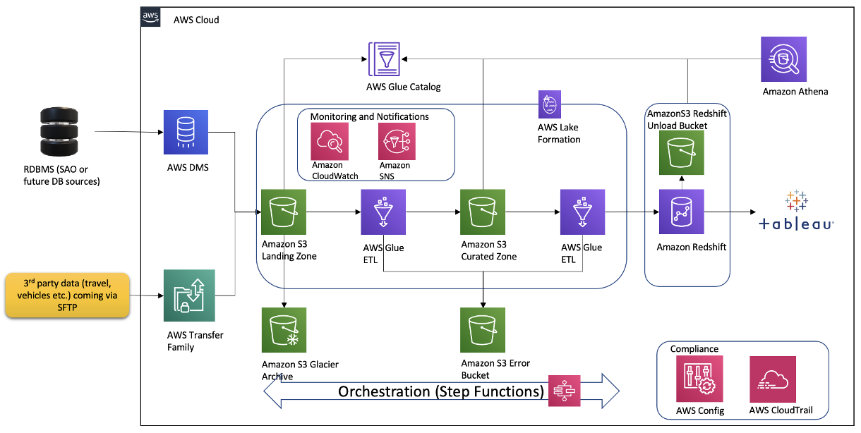
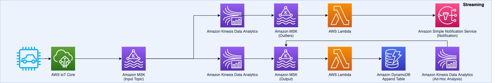
The following diagram illustrates the data ingestion workflow.

Data Ingestion Workflow

The team needed to quickly populate millions of Kafka messages in the dev/test environment to achieve this. To expedite the process, we (the team) opted to use Amazon Managed Streaming for Apache Kafka (Amazon MSK), which makes it simple to ingest and process streaming data in real time, and we were up and running in under a day.

To generate test data that resembled production data, the AWS Data Lab team created a custom Python script that evenly populated over 1.2 billion messages across several Kafka partitions. To match the production setup in the development account, we had to increase the cloud quota limit via a support ticket.

We used Amazon MSK and the Spark Structured Streaming capability in Amazon EMR to ingest and process the incoming Kafka messages with high throughput and low latency. Specifically, we inserted the data from the source into EMR clusters at a maximum incoming rate of 150 million Kafka messages every 5 minutes, with each Kafka message holding 7–25 log data records.

To store the data, we chose to use Apache Hudi as the table format. We opted for Hudi because it’s an open-source data management framework that provides record-level insert, update, and delete capabilities on top of an immutable storage layer like Amazon Simple Storage Service (Amazon S3). Additionally, Hudi is optimized for handling large datasets and works well with Spark Structured Streaming, which was already being used at Zoom.

After 150 million messages were buffered, we processed the messages using Spark Structured Streaming on Amazon EMR and wrote the data into Amazon S3 in Apache Hudi-compatible format every 5 minutes. We first flattened the message array, creating a single record from the nested array of messages. Then we added a unique key, known as the Hudi record key, to each message. This key allows Hudi to perform record-level insert, update, and delete operations on the data. We also extracted the field values, including the Hudi partition keys, from incoming messages.

This architecture allowed end-users to query the data stored in Amazon S3 using Amazon Athena with the AWS Glue Data Catalog or using Apache Hive and Presto.

Data deletion workflow

The following diagram illustrates the data deletion workflow.

Data Deletion Workflow

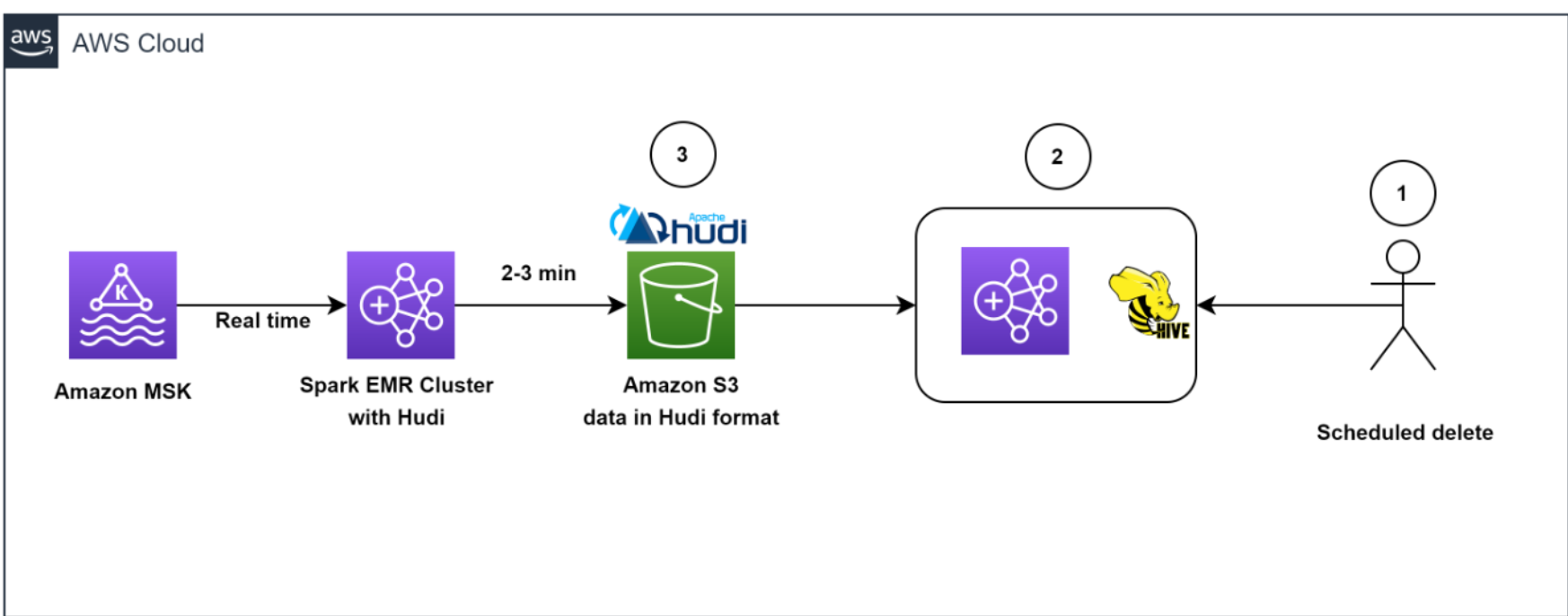
Our architecture allowed for efficient data deletions. To help comply with the customer-initiated data retention policy for GDPR deletes, scheduled jobs ran daily to identify the data to be deleted in batch mode.

We then spun up a transient EMR cluster to run the GDPR upsert job to delete the records. The data was stored in Amazon S3 in Hudi format, and Hudi’s built-in index allowed us to efficiently delete records using bloom filters and file ranges. Because only those files that contained the record keys needed to be read and rewritten, it only took about 1–2 minutes to delete 1,000 records out of the 1 billion records, which had previously taken hours to complete as entire partitions were read.

Overall, our solution enabled efficient deletion of data, which provided an additional layer of data security that was critical for Zoom, in light of its GDPR requirements.

Architecting to optimize scale, performance, and cost

In this section, we share the following strategies Zoom took to optimize scale, performance, and cost:

  • Optimizing ingestion
  • Optimizing throughput and Amazon EMR utilization
  • Decoupling ingestion and GDPR deletion using EMRFS
  • Efficient deletes with Apache Hudi
  • Optimizing for low-latency reads with Apache Hudi
  • Monitoring

Optimizing ingestion

To keep the storage in Kafka lean and optimal, as well as to get a real-time view of data, we created a Spark job to read incoming Kafka messages in batches of 150 million messages and wrote to Amazon S3 in Hudi-compatible format every 5 minutes. Even during the initial stages of the iteration, when we hadn’t started scaling and tuning yet, we were able to successfully load all Kafka messages consistently under 2.5 minutes using the Amazon EMR runtime for Apache Spark.

Optimizing throughput and Amazon EMR utilization

We launched a cost-optimized EMR cluster and switched from uniform instance groups to using EMR instance fleets. We chose instance fleets because we needed the flexibility to use Spot Instances for task nodes and wanted to diversify the risk of running out of capacity for a specific instance type in our Availability Zone.

We started experimenting with test runs by first changing the number of Kafka partitions from 400 to 1,000, and then changing the number of task nodes and instance types. Based on the results of the run, the AWS team came up with the recommendation to use Amazon EMR with three core nodes (r5.16xlarge (64 vCPUs each)) and 18 task nodes using Spot fleet instances (a combination of r5.16xlarge (64 vCPUs), r5.12xlarge (48 vCPUs), r5.8xlarge (32 vCPUs)). These recommendations helped Zoom to reduce their Amazon EMR costs by more than 80% while meeting their desired performance goals of ingesting 150 million Kafka messages under 5 minutes.

Decoupling ingestion and GDPR deletion using EMRFS

A well-known benefit of separation of storage and compute is that you can scale the two independently. But a not-so-obvious advantage is that you can decouple continuous workloads from sporadic workloads. Previously data was stored in HDFS. Resource-intensive GDPR delete jobs and data movement jobs would compete for resources with the stream ingestion, causing a backlog of more than 5 hours in upstream Kafka clusters, which was close to filling up the Kafka storage (which only had 6 hours of data retention) and potentially causing data loss. Offloading data from HDFS to Amazon S3 allowed us the freedom to launch independent transient EMR clusters on demand to perform data deletion, helping to ensure that the ongoing data ingestion from Kafka into Amazon EMR is not starved for resources. This enabled the system to ingest data every 5 minutes and complete each Spark Streaming read in 2–3 minutes. Another side effect of using EMRFS is a cost-optimized cluster, because we removed reliance on Amazon Elastic Block Store (Amazon EBS) volumes for over 300 TB storage that was used for three copies (including two replicas) of HDFS data. We now pay for only one copy of the data in Amazon S3, which provides 11 9s of durability and is relatively inexpensive storage.

Efficient deletes with Apache Hudi

What about the conflict between ingest writes and GDPR deletes when running concurrently? This is where the power of Apache Hudi stands out.

Apache Hudi provides a table format for data lakes with transactional semantics that enables the separation of ingestion workloads and updates when run concurrently. The system was able to consistently delete 1,000 records in less than a minute. There were some limitations in concurrent writes in Apache Hudi 0.7.0, but the Amazon EMR team quickly addressed this by back-porting Apache Hudi 0.8.0, which supports optimistic concurrency control, to the current (at the time of the AWS Data Lab collaboration) Amazon EMR 6.4 release. This saved time in testing and allowed for a quick transition to the new version with minimal testing. This enabled us to query the data directly using Athena quickly without having to spin up a cluster to run ad hoc queries, as well as to query the data using Presto, Trino, and Hive. The decoupling of the storage and compute layers provided the flexibility to not only query data across different EMR clusters, but also delete data using a completely independent transient cluster.

Optimizing for low-latency reads with Apache Hudi

To optimize for low-latency reads with Apache Hudi, we needed to address the issue of too many small files being created within Amazon S3 due to the continuous streaming of data into the data lake.

We utilized Apache Hudi’s features to tune file sizes for optimal querying. Specifically, we reduced the degree of parallelism in Hudi from the default value of 1,500 to a lower number. Parallelism refers to the number of threads used to write data to Hudi; by reducing it, we were able to create larger files that were more optimal for querying.

Because we needed to optimize for high-volume streaming ingestion, we chose to implement the merge on read table type (instead of copy on write) for our workload. This table type allowed us to quickly ingest the incoming data into delta files in row format (Avro) and asynchronously compact the delta files into columnar Parquet files for fast reads. To do this, we ran the Hudi compaction job in the background. Compaction is the process of merging row-based delta files to produce new versions of columnar files. Because the compaction job would use additional compute resources, we adjusted the degree of parallelism for insertion to a lower value of 1,000 to account for the additional resource usage. This adjustment allowed us to create larger files without sacrificing performance throughput.

Overall, our approach to optimizing for low-latency reads with Apache Hudi allowed us to better manage file sizes and improve the overall performance of our data lake.

Monitoring

The team monitored MSK clusters with Prometheus (an open-source monitoring tool). Additionally, we showcased how to monitor Spark streaming jobs using Amazon CloudWatch metrics. For more information, refer to Monitor Spark streaming applications on Amazon EMR.

Outcomes

The collaboration between Zoom and the AWS Data Lab demonstrated significant improvements in data ingestion, processing, storage, and deletion using an architecture with Amazon EMR and Apache Hudi. One key benefit of the architecture was a reduction in infrastructure costs, which was achieved through the use of cloud-native technologies and the efficient management of data storage. Another benefit was an improvement in data management capabilities.

We showed that the costs of EMR clusters can be reduced by about 82% while bringing the storage costs down by about 90% compared to the prior HDFS-based architecture. All of this while making the data available in the data lake within 5 minutes of ingestion from the source. We also demonstrated that data deletions from a data lake containing multiple petabytes of data can be performed much more efficiently. With our optimized approach, we were able to delete approximately 1,000 records in just 1–2 minutes, as compared to the previously required 3 hours or more.

Conclusion

In conclusion, the log analytics process, which involves collecting, processing, storing, analyzing, and deleting log data from various sources such as servers, applications, and devices, is critical to aid organizations in working to meet their service resiliency, security, performance monitoring, troubleshooting, and compliance needs, such as GDPR.

This post shared what Zoom and the AWS Data Lab team have accomplished together to solve critical data pipeline challenges, and Zoom has extended the solution further to optimize extract, transform, and load (ETL) jobs and resource efficiency. However, you can also use the architecture patterns presented here to quickly build cost-effective and scalable solutions for other use cases. Please reach out to your AWS team for more information or contact Sales.


About the Authors

Sekar Srinivasan is a Sr. Specialist Solutions Architect at AWS focused on Big Data and Analytics. Sekar has over 20 years of experience working with data. He is passionate about helping customers build scalable solutions modernizing their architecture and generating insights from their data. In his spare time he likes to work on non-profit projects focused on underprivileged Children’s education.

Chandra DhandapaniChandra Dhandapani is a Senior Solutions Architect at AWS, where he specializes in creating solutions for customers in Analytics, AI/ML, and Databases. He has a lot of experience in building and scaling applications across different industries including Healthcare and Fintech. Outside of work, he is an avid traveler and enjoys sports, reading, and entertainment.

Amit Kumar Agrawal is a Senior Solutions Architect at AWS, based out of San Francisco Bay Area. He works with large strategic ISV customers to architect cloud solutions that address their business challenges. During his free time he enjoys exploring the outdoors with his family.

Viral Shah is a Analytics Sales Specialist working with AWS for 5 years helping customers to be successful in their data journey. He has over 20+ years of experience working with enterprise customers and startups, primarily in the data and database space. He loves to travel and spend quality time with his family.

How Encored Technologies built serverless event-driven data pipelines with AWS

Post Syndicated from Younggu Yun original https://aws.amazon.com/blogs/big-data/how-encored-technologies-built-serverless-event-driven-data-pipelines-with-aws/

This post is a guest post co-written with SeonJeong Lee, JaeRyun Yim, and HyeonSeok Yang from Encored Technologies.

Encored Technologies (Encored) is an energy IT company in Korea that helps their customers generate higher revenue and reduce operational costs in renewable energy industries by providing various AI-based solutions. Encored develops machine learning (ML) applications predicting and optimizing various energy-related processes, and their key initiative is to predict the amount of power generated at renewable energy power plants.

In this post, we share how Encored runs data engineering pipelines for containerized ML applications on AWS and how they use AWS Lambda to achieve performance improvement, cost reduction, and operational efficiency. We also demonstrate how to use AWS services to ingest and process GRIB (GRIdded Binary) format data, which is a file format commonly used in meteorology to store and exchange weather and climate data in a compressed binary form. It allows for efficient data storage and transmission, as well as easy manipulation of the data using specialized software.

Business and technical challenge

Encored is expanding their business into multiple countries to provide power trading services for end customers. The amount of data and the number of power plants they need to collect data are rapidly increasing over time. For example, the volume of data required for training one of the ML models is more than 200 TB. To meet the growing requirements of the business, the data science and platform team needed to speed up the process of delivering model outputs. As a solution, Encored aimed to migrate existing data and run ML applications in the AWS Cloud environment to efficiently process a scalable and robust end-to-end data and ML pipeline.

Solution overview

The primary objective of the solution is to develop an optimized data ingestion pipeline that addresses the scaling challenges related to data ingestion. During its previous deployment in an on-premises environment, the time taken to process data from ingestion to preparing the training dataset exceeded the required service level agreement (SLA). One of the input datasets required for ML models is weather data supplied by the Korea Meteorological Administration (KMA). In order to use the GRIB datasets for the ML models, Encored needed to prepare the raw data to make it suitable for building and training ML models. The first step was to convert GRIB to the Parquet file format.

Encored used Lambda to run an existing data ingestion pipeline built in a Linux-based container image. Lambda is a compute service that lets you run code without provisioning or managing servers. Lambda runs your code on a high-availability compute infrastructure and performs all of the administration of the compute resources, including server and operating system maintenance, capacity provisioning and automatic scaling, and logging. AWS Lambda is triggered to ingest and process GRIB data files when they are uploaded to Amazon Simple Storage Service (Amazon S3). Once the files are processed, they are stored in Parquet format in the other S3 bucket. Encored receives GRIB files throughout the day, and whenever new files arrive, an AWS Lambda function runs a container image registered in Amazon Elastic Container Registry (ECR). This event-based pipeline triggers a customized data pipeline that is packaged in a container-based solution. Leveraging Amazon AWS Lambda, this solution is cost-effective, scalable, and high-performing.Encored uses Python as their preferred language.

The following diagram illustrates the solution architecture.

Lambda-data-pipeline

For data-intensive tasks such as extract, transform, and load (ETL) jobs and ML inference, Lambda is an ideal solution because it offers several key benefits, including rapid scaling to meet demand, automatic scaling to zero when not in use, and S3 event triggers that can initiate actions in response to object-created events. All this contributes to building a scalable and cost-effective data event-driven pipeline. In addition to these benefits, Lambda allows you to configure ephemeral storage (/tmp) between 512–10,240 MB. Encored used this storage for their data application when reading or writing data, enabling them to optimize performance and cost-effectiveness. Furthermore, Lambda’s pay-per-use pricing model means that users only pay for the compute time in use, making it a cost-effective solution for a wide range of use cases.

Prerequisites

For this walkthrough, you should have the following:

Build your application required for your Docker image

The first step is to develop an application that can ingest and process files. This application reads the bucket name and object key passed from a trigger added to Lambda function. The processing logic involves three parts: downloading the file from Amazon S3 into ephemeral storage (/tmp), parsing the GRIB formatted data, and saving the parsed data to Parquet format.

The customer has a Python script (for example, app.py) that performs these tasks as follows:

import os
import tempfile
import boto3
import numpy as np
import pandas as pd
import pygrib

s3_client = boto3.client('s3')
def handler(event, context):
    try:
        # Get trigger file name
        bucket_name = event["Records"][0]["s3"]["bucket"]["name"]
        s3_file_name = event["Records"][0]["s3"]["object"]["key"]

        # Handle temp files: all temp objects are deleted when the with-clause is closed
        with tempfile.NamedTemporaryFile(delete=True) as tmp_file:
            # Step1> Download file from s3 into temp area
            s3_file_basename = os.path.basename(s3_file_name)
            s3_file_dirname = os.path.dirname(s3_file_name)
            local_filename = tmp_file.name
            s3_client.download_file(
                Bucket=bucket_name,
                Key=f"{s3_file_dirname}/{s3_file_basename}",
                Filename=local_filename
            )

            # Step2> Parse – GRIB2 
            grbs = pygrib.open(local_filename)
            list_of_name = []
            list_of_values = []
            for grb in grbs:
                list_of_name.append(grb.name)
                list_of_values.append(grb.values)
            _, lat, lon = grb.data()
            list_of_name += ["lat", "lon"]
            list_of_values += [lat, lon]
            grbs.close()

            dat = pd.DataFrame(
                np.transpose(np.stack(list_of_values).reshape(len(list_of_values), -1)),
                columns=list_of_name,
            )

        # Step3> To Parquet
        s3_dest_uri = S3path
        dat.to_parquet(s3_dest_uri, compression="snappy")

    except Exception as err:
        print(err)

Prepare a Docker file

The second step is to create a Docker image using an AWS base image. To achieve this, you can create a new Dockerfile using a text editor on your local machine. This Dockerfile should contain two environment variables:

  • LAMBDA_TASK_ROOT=/var/task
  • LAMBDA_RUNTIME_DIR=/var/runtime

It’s important to install any dependencies under the ${LAMBDA_TASK_ROOT} directory alongside the function handler to ensure that the Lambda runtime can locate them when the function is invoked. Refer to the available Lambda base images for custom runtime for more information.

FROM public.ecr.aws/lambda/python:3.8

# Install the function's dependencies using file requirements.txt
# from your project folder.

COPY requirements.txt  .
RUN pip3 install -r requirements.txt --target "${LAMBDA_TASK_ROOT}"

# Copy function code
COPY app.py ${LAMBDA_TASK_ROOT}

# Set the CMD to your handler (could also be done as a parameter override outside of the Dockerfile)
CMD [ "app.handler" ]

Build a Docker image

The third step is to build your Docker image using the docker build command. When running this command, make sure to enter a name for the image. For example:

docker build -t process-grib .

In this example, the name of the image is process-grib. You can choose any name you like for your Docker image.

Upload the image to the Amazon ECR repository

Your container image needs to reside in an Amazon Elastic Container Registry (Amazon ECR) repository. Amazon ECR is a fully managed container registry offering high-performance hosting, so you can reliably deploy application images and artifacts anywhere. For instructions on creating an ECR repository, refer to Creating a private repository.

The first step is to authenticate the Docker CLI to your ECR registry as follows:

aws ecr get-login-password --region ap-northeast-2 | docker login --username AWS --password-stdin 123456789012.dkr.ecr.ap-northeast-2.amazonaws.com 

The second step is to tag your image to match your repository name, and deploy the image to Amazon ECR using the docker push command:

docker tag  hello-world:latest 123456789012.dkr.ecr. ap-northeast-2.amazonaws.com/hello-world:latest
docker push 123456789012.dkr.ecr. ap-northeast-2.amazonaws.com/hello-world:latest     

Deploy Lambda functions as container images

To create your Lambda function, complete the following steps:

  1. On the Lambda console, choose Functions in the navigation pane.
  2. Choose Create function.
  3. Choose the Container image option.
  4. For Function name, enter a name.
  5. For Container image URI, provide a container image. You can enter the ECR image URI or browse for the ECR image.
  6. Under Container image overrides, you can override configuration settings such as the entry point or working directory that are included in the Dockerfile.
  7. Under Permissions, expand Change default execution role.
  8. Choose to create a new role or use an existing role.
  9. Choose Create function.

Key considerations

To handle a large amount of data concurrently and quickly, Encored needed to store GRIB formatted files in the ephemeral storage (/tmp) that comes with Lambda. To achieve this requirement, Encored used tempfile.NamedTemporaryFile, which allows users to create temporary files easily that are deleted when no longer needed. With Lambda, you can configure ephemeral storage between 512 MB–10,240 MB for reading or writing data, allowing you to run ETL jobs, ML inference, or other data-intensive workloads.

Business outcome

Hyoseop Lee (CTO at Encored Technologies) said, “Encored has experienced positive outcomes since migrating to AWS Cloud. Initially, there was a perception that running workloads on AWS would be more expensive than using an on-premises environment. However, we discovered that this was not the case once we started running our applications on AWS. One of the most fascinating aspects of AWS services is the flexible architecture options it provides for processing, storing, and accessing large volumes of data that are only required infrequently.”

Conclusion

In this post, we covered how Encored built serverless data pipelines with Lambda and Amazon ECR to achieve performance improvement, cost reduction, and operational efficiency.

Encored successfully built an architecture that will support their global expansion and enhance technical capabilities through AWS services and the AWS Data Lab program. Based on the architecture and various internal datasets Encored has consolidated and curated, Encored plans to provide renewable energy forecasting and energy trading services.

Thanks for reading this post and hopefully you found it useful. To accelerate your digital transformation with ML, AWS is available to support you by providing prescriptive architectural guidance on a particular use case, sharing best practices, and removing technical roadblocks. You’ll leave the engagement with an architecture or working prototype that is custom fit to your needs, a path to production, and deeper knowledge of AWS services. Please contact your AWS Account Manager or Solutions Architect to get started. If you don’t have an AWS Account Manager, please contact Sales.

To learn more about ML inference use cases with Lambda, check out the following blog posts:

These resources will provide you with valuable insights and practical examples of how to use Lambda for ML inference.


About the Authors

leeSeonJeong Lee is the Head of Algorithms at Encored. She is a data practitioner who finds peace of mind from beautiful codes and formulas.

yimJaeRyun Yim is a Senior Data Scientist at Encored. He is striving to improve both work and life by focusing on simplicity and essence in my work.

yangHyeonSeok Yang is the platform team lead at Encored. He always strives to work with passion and spirit to keep challenging like a junior developer, and become a role model for others.

youngguYounggu Yun works at AWS Data Lab in Korea. His role involves helping customers across the APAC region meet their business objectives and overcome technical challenges by providing prescriptive architectural guidance, sharing best practices, and building innovative solutions together.

How Huron built an Amazon QuickSight Asset Catalogue with AWS CDK Based Deployment Pipeline

Post Syndicated from Corey Johnson original https://aws.amazon.com/blogs/big-data/how-huron-built-an-amazon-quicksight-asset-catalogue-with-aws-cdk-based-deployment-pipeline/

This is a guest blog post co-written with Corey Johnson from Huron.

Having an accurate and up-to-date inventory of all technical assets helps an organization ensure it can keep track of all its resources with metadata information such as their assigned oners, last updated date, used by whom, how frequently and more. It helps engineers, analysts and businesses access the most up-to-date release of the software asset that bring accuracy to the decision-making process. By keeping track of this information, organizations will be able to identify technology gaps, refresh cycles, and expire assets as needed for archival.

In addition, an inventory of all assets is one of the foundational elements of an organization that facilitates the security and compliance team to audit the assets for improving privacy, security posture and mitigate risk to ensure the business operations run smoothly. Organizations may have different ways of maintaining an asset inventory, that may be an Excel spreadsheet or a database with a fully automated system to keep it up-to-date, but with a common objective of keeping it accurate. Even if organizations can follow manual approaches to update the inventory records but it is recommended to build automation, so that it is accurate at any point of time.

The DevOps practices which revolutionized software engineering in the last decade have yet to come to the world of Business Intelligence solutions. Business intelligence tools by their nature use a paradigm of UI driven development with code-first practices being secondary or nonexistent. As the need for applications that can leverage the organizations internal and client data increases, the same DevOps practices (BIOps) can drive and delivery quality insights more reliably

In this post, we walk you through a solution that Huron and manage lifecycle for all Amazon QuickSight resources across the organization by collaborating with AWS Data Lab Resident Architect & AWS Professional Services team.

About Huron

Huron is a global professional services firm that collaborates with clients to put possible into practice by creating sound strategies, optimizing operations, accelerating digital transformation, and empowering businesses and their people to own their future. By embracing diverse perspectives, encouraging new ideas, and challenging the status quo, Huron creates sustainable results for the organizations we serve. To help address its clients’ growing cloud needs, Huron is an AWS Partner.

Use Case Overview

Huron’s Business Intelligence use case represents visualizations as a service, where Huron has core set of visualizations and dashboards available as products for its customers. The products exist in different industry verticals (healthcare, education, commercial) with independent development teams. Huron’s consultants leverage the products to provide insights as part of consulting engagements. The insights from the product help Huron’s consultants accelerate their customer’s transformation. As part of its overall suite of offerings, there are product dashboards that are featured in a software application following a standardized development lifecycle. In addition, these product dashboards may be forked for customer-specific customization to support a consulting engagement while still consuming from Huron’s productized data assets and datasets. In the next stage of the cycle, Huron’s consultants experiment with new data sources and insights that in turn fed back into the product dashboards.

When changes are made to a product analysis, challenges arise when a base reference analysis gets updated because of new feature releases or bug fixes, and all the customer visualizations that are created from it also need to be updated. To maintain the integrity of embedded visualizations, all metadata and lineage must be available to the parent application. This access to the metadata supports the need for updating visuals based on changes as well as automating row and column level security ensuring customer data is properly governed.

In addition, few customers request customizations on top of the base visualizations, for which Huron team needs to create a replica of the base reference and then customize it for the customer. These are maintained by Huron’s in the field consultants rather than the product development team. These customer specific visualizations create operational overhead because they require Huron to keep track of new customer specific visualizations and maintain them for future releases when the product visuals change.

Huron leverages Amazon QuickSight for their Business Intelligence (BI) reporting needs, enabling them to embed visualizations at scale with higher efficiency and lower cost. A large attraction for Huron to adopt QuickSight came from the forward-looking API capabilities that enable and set the foundation for a BIOps culture and technical infrastructure. To address the above requirement, Huron Global Product team decided to build a QuickSight Asset Tracker and QuickSight Asset Deployment Pipeline.

The QuickSight Asset tracker serves as a catalogue of all QuickSight resources (datasets, analysis, templates, dashboards etc.) with its interdependent relationship. It will help;

  • Create an inventory of all QuickSight resources across all business units
  • Enable dynamic embedding of visualizations and dashboards based on logged in user
  • Enable dynamic row and column level security on the dashboards and visualizations based on the logged-in user
  • Meet compliance and audit requirements of the organization
  • Maintain the current state of all customer specific QuickSight resources

The solution integrates an AWS CDK based pipeline to deploy QuickSight Assets that:

  • Supports Infrastructure-as-a-code for QuickSight Asset Deployment and enables rollbacks if required.
  • Enables separation of development, staging and production environments using QuickSight folders that reduces the burden of multi-account management of QuickSight resources.
  • Enables a hub-and-spoke model for Data Access in multiple AWS accounts in a data mesh fashion.

QuickSight Asset Tracker and QuickSight Asset Management Pipeline – Architecture Overview

The QuickSight Asset Tracker was built as an independent service, which was deployed in a shared AWS service account that integrated Amazon Aurora Serverless PostgreSQL to store metadata information, AWS Lambda as the serverless compute and Amazon API Gateway to provide the REST API layer.

It also integrated AWS CDK and AWS CloudFormation to deploy the product and customer specific QuickSight resources and keep them in consistent and stable state. The metadata of QuickSight resources, created using either AWS console or the AWS CDK based deployment were maintained in Amazon Aurora database through the QuickSight Asset Tracker REST API service.

The CDK based deployment pipeline is triggered via a CI/CD pipeline which performs the following functions:

  1. Takes the ARN of the QuickSight assets (dataset, analysis, etc.)
  2. Describes the asset and dependent resources (if selected)
  3. Creates a copy of the resource in another environment (in this case a QuickSight folder) using CDK

The solution architecture integrated the following AWS services.

  • Amazon Aurora Serverless integrated as the backend database to store metadata information of all QuickSight resources with customer and product information they are related to.
  • Amazon QuickSight as the BI service using which visualization and dashboards can be created and embedded into the online applications.
  • AWS Lambda as the serverless compute service that gets invoked by online applications using Amazon API Gateway service.
  • Amazon SQS to store customer request messages, so that the AWS CDK based pipeline can read from it for processing.
  • AWS CodeCommit is integrated to store the AWS CDK deployment scripts and AWS CodeBuild, AWS CloudFormation integrated to deploy the AWS resources using an infrastructure as a code approach.
  • AWS CloudTrail is integrated to audit user actions and trigger Amazon EventBridge rules when a QuickSight resource is created, updated or deleted, so that the QuickSight Asset Tracker is up-to-date.
  • Amazon S3 integrated to store metadata information, which is used by AWS CDK based pipeline to deploy the QuickSight resources.
  • AWS LakeFormation enables cross-account data access in support of the QuickSight Data Mesh

The following provides a high-level view of the solution architecture.

Architecture Walkthrough:

The following provides a detailed walkthrough of the above architecture.

  • QuickSight Dataset, Template, Analysis, Dashboard and visualization relationships:
    • Steps 1 to 2 represent QuickSight reference analysis reading data from different data sources that may include Amazon S3, Amazon Athena, Amazon Redshift, Amazon Aurora or any other JDBC based sources.
    • Step 3 represents QuickSight templates being created from reference analysis when a customer specific visualization needs to be created and step 4.1 to 4.2 represents customer analysis and dashboards being created from the templates.
    • Steps 7 to 8 represent QuickSight visualizations getting generated from analysis/dashboard and step 6 represents the customer analysis/dashboard/visualizations referring their own customer datasets.
    • Step 10 represents a new fork being created from the base reference analysis for a specific customer, which will create a new QuickSight template and reference analysis for that customer.
    • Step 9 represents end users accessing QuickSight visualizations.
  • Asset Tracker REST API service:
    • Step 15.2 to 15.4 represents the Asset Tracker service, which is deployed in a shared AWS service account, where Amazon API Gateway provides the REST API layer, which invokes AWS Lambda function to read from or write to backend Aurora database (Aurora Serverless v2 – PostgreSQL engine). The database captures all relationship metadata between QuickSight resources, its owners, assigned customers and products.
  • Online application – QuickSight asset discovery and creation
    • Step 15.1 represents the front-end online application reading QuickSight metadata information from the Asset Tracker service to help customers or end users discover visualizations available and be able to dynamically render based on the user login.
    • Step 11 to 12 represents the online application requesting creation of new QuickSight resources, which pushes requests to Amazon SQS and then AWS Lambda triggers AWS CodeBuild to deploy new QuickSight resources. Step 13.1 and 13.2 represents the CDK based pipeline maintaining the QuickSight resources to keep them in a consistent state. Finally, the AWS CDK stack invokes the Asset Tracker service to update its metadata as represented in step 13.3.
  • Tracking QuickSight resources created outside of the AWS CDK Stack
    • Step 14.1 represents users creating QuickSight resources using the AWS Console and step 14.2 represents that activity getting logged into AWS CloudTrail.
    • Step 14.3 to 14.5 represents triggering EventBridge rule for CloudTrail activities that represents QuickSight resource being created, updated or deleted and then invoke the Asset Tracker REST API to register the QuickSight resource metadata.

Architecture Decisions:

The following are few architecture decisions we took while designing the solution.

  • Choosing Aurora database for Asset Tracker: We have evaluated Amazon Neptune for the Asset Tracker database as most of the metadata information we capture are primarily maintaining relationship between QuickSight resources. But when we looked at the query patterns, we found the query pattern is always just one level deep to find who is the parent of a specific QuickSight resource and that can be solved with a relational database’s Primary Key / Foreign Key relationship and with simple self-join SQL query. Knowing the query pattern does not require a graph database, we decided to go with Amazon Aurora to keep it simple, so that we can avoid introducing a new database technology and can reduce operational overhead of maintaining it. In future as the use case evolve, we can evaluate the need for a Graph database and plan for integrating it. For Amazon Aurora, we choose Amazon Aurora Serverless as the usage pattern is not consistent to reserve a server capacity and the serverless tech stack will help reduce operational overhead.
  • Decoupling Asset Tracker as a common REST API service: The Asset Tracker has future scope to be a centralized metadata layer to keep track of all the QuickSight resources across all business units of Huron. So instead of each business unit having its own metadata database, if we build it as a service and deploy it in a shared AWS service account, then we will get benefit from reduced operational overhead, duplicate infrastructure cost and will be able to get a consolidated view of all assets and their integrations. The service provides the ability of applications to consume metadata about the QuickSight assets and then apply their own mapping of security policies to the assets based on their own application data and access control policies.
  • Central QuickSight account with subfolder for environments: The choice was made to use a central account which reduces developer friction of having multiple accounts with multiple identities, end users having to manage multiple accounts and access to resources. QuickSight folders allow for appropriate permissions for separating “environments”. Furthermore, by using folder-based sharing with QuickSight groups, users with appropriate permissions already have access to the latest versions of QuickSight assets without having to share their individual identities.

The solution included an automated Continuous Integration (CI) and Continuous Deployment (CD) pipeline to deploy the resources from development to staging and then finally to production. The following provides a high-level view of the QuickSight CI/CD deployment strategy.

Aurora Database Tables and Reference Analysis update flow

The following are the database tables integrated to capture the QuickSight resource metadata.

  • QS_Dataset: This captures metadata of all QuickSight datasets that are integrated in the reference analysis or customer analysis. This includes AWS ARN (Amazon Resource Name), data source type, ID and more.
  • QS_Template: This table captures metadata of all QuickSight templates, from which customer analysis and dashboards will be created. This includes AWS ARN, parent reference analysis ID, name, version number and more.
  • QS_Folder: This table captures metadata about QuickSight folders which logically groups different visualizations. This includes AWS ARN, name, and description.
  • QS_Analysis: This table captures metadata of all QuickSight analysis that includes AWS ARN, name, type, dataset IDs, parent template ID, tags, permissions and more.
  • QS_Dashboard: This table captures metadata information of QuickSight dashboards that includes AWS ARN, parent template ID, name, dataset IDs, tags, permissions and more.
  • QS_Folder_Asset_Mapping: This table captures folder to QuickSight asset mapping that includes folder ID, Asset ID, and asset type.

As the solution moves to the next phase of implementation, we plan to introduce additional database tables to capture metadata information about QuickSight sheets and asset mapping to customers and products. We will extend the functionality to support visual based embedding to enable truly integrated customer data experiences where embedded visuals mesh with the native content on a web page.

While explaining the use case, we have highlighted it creates a challenge when a base reference analysis gets updated and we need to track the templates that are inherited from it make sure the change is pushed to the linked customer analysis and dashboards. The following example scenarios explains, how the database tables change when a reference analysis is updated.

Example Scenario: When “reference analysis” is updated with a new release

When a base reference analysis is updated because of a new feature release, then a new QuickSight reference analysis and template needs to be created. Then we need to update all customer analysis and dashboard records to point to the new template ID to form the lineage.

The following sequential steps represent the database changes that needs to happen.

  • Insert a new record to the “Analysis” table to represent the new reference analysis creation.
  • Insert a new record to the “Template” table with new reference analysis ID as parent, created in step 1.
  • Retrieve “Analysis” and “Dashboard” table records that points to previous template ID and then update those records with the new template ID, created in step 2.

How will it enable a more robust embedding experience

The QuickSight asset tracker integration with Huron’s products provide users with a personalized, secure and modern analytics experience. When user’s login through Huron’s online application, it will use logged in user’s information to dynamically identify the products they are mapped to and then render the QuickSight visualizations & dashboards that the user is entitled to see. This will improve user experience, enable granular permission management and will also increase performance.

How AWS collaborated with Huron to help build the solution

AWS team collaborated with Huron team to design and implement the solution. AWS Data Lab Resident Architect collaborated with Huron’s lead architect for initial architecture design that compared different options for integration and deriving tradeoffs between them, before finalizing the final architecture. Then with the help of AWS Professional service engineer, we could build the base solution that can be extended by Huron team to roll it out to all business units and integrate additional reporting features on top of it.

The AWS Data Lab Resident Architect program provides AWS customers with guidance in refining and executing their data strategy and solutions roadmap. Resident Architects are dedicated to customers for 6 months, with opportunities for extension, and help customers (Chief Data Officers, VPs of Data Architecture, and Builders) make informed choices and tradeoffs about accelerating their data and analytics workloads and implementation.

The AWS Professional Services organization is a global team of experts that can help customers realize their desired business outcomes when using the AWS Cloud. The Professional Services team work together with customer’s team and their chosen member of the AWS Partner Network (APN) to execute their enterprise cloud computing initiatives.

Next Steps

Huron has rolled out the solution for one business unit and as a next step we plan to roll it out to all business units, so that the asset tracker service is populated with assets available across all business units of the organization to provide consolidated view.

In addition, Huron will be building a reporting layer on top of the Amazon Aurora asset tracker database, so that the leadership has a way to discover assets by business unit, by owner, created between specific date range or the reports that are not updated since a while.

Once the asset tracker is populated with all QuickSight assets, it will be integrated into the front-end online application that can help end users discover existing assets and request creation of new assets.

Newer QuickSight API’s such as assets-as-a-bundle and assets-as-code further accelerate the capabilities of the service by improving the development velocity and reliability of making changes.

Conclusion

This blog explained how Huron built an Asset Tracker to keep track of all QuickSight resources across the organization. This solution may provide a reference to other organizations who would like to build an inventory of visualization reports, ML models or other technical assets. This solution leveraged Amazon Aurora as the primary database, but if an organization would also like to build a detailed lineage of all the assets to understand how they are interrelated then they can consider integrating Amazon Neptune as an alternate database too.

If you have a similar use case and would like to collaborate with AWS Data Analytics Specialist Architects to brainstorm on the architecture, rapidly prototype it and implement a production ready solution then connect with your AWS Account Manager or AWS Solution Architect to start an engagement with AWS Data Lab team.


About the Authors

Corey Johnson is the Lead Data Architect at Huron, where he leads its data architecture for their Global Products Data and Analytics initiatives.

Sakti Mishra is a Principal Data Analytics Architect at AWS, where he helps customers modernize their data architecture, help define end to end data strategy including data security, accessibility, governance, and more. He is also the author of the book Simplify Big Data Analytics with Amazon EMR. Outside of work, Sakti enjoys learning new technologies, watching movies, and visiting places with family.

How CyberSolutions built a scalable data pipeline using Amazon EMR Serverless and the AWS Data Lab

Post Syndicated from Constantin Scoarță original https://aws.amazon.com/blogs/big-data/how-cybersolutions-built-a-scalable-data-pipeline-using-amazon-emr-serverless-and-the-aws-data-lab/

This post is co-written by Constantin Scoarță and Horațiu Măiereanu from CyberSolutions Tech.

CyberSolutions is one of the leading ecommerce enablers in Germany. We design, implement, maintain, and optimize award-winning ecommerce platforms end to end. Our solutions are based on best-in-class software like SAP Hybris and Adobe Experience Manager, and complemented by unique services that help automate the pricing and sourcing processes.

We have built data pipelines to process, aggregate, and clean our data for our forecasting service. With the growing interest in our services, we wanted to scale our batch-based data pipeline to process more historical data on a daily basis and yet remain performant, cost-efficient, and predictable. To meet our requirements, we have been exploring the use of Amazon EMR Serverless as a potential solution.

To accelerate our initiative, we worked with the AWS Data Lab team. They offer joint engineering engagements between customers and AWS technical resources to create tangible deliverables that accelerate data and analytics initiatives. We chose to work through a Build Lab, which is a 2–5-day intensive build with a technical customer team.

In this post, we share how we engaged with the AWS Data Lab program to build a scalable and performant data pipeline using EMR Serverless.

Use case

Our forecasting and recommendation algorithm is fed with historical data, which needs to be curated, cleaned, and aggregated. Our solution was based on AWS Glue workflows orchestrating a set of AWS Glue jobs, which worked fine for our requirements. However, as our use case developed, it required more computations and bigger datasets, resulting into unpredictable performance and cost.

This pipeline performs daily extracts from our data warehouse and a few other systems, curates the data, and does some aggregations (such as daily average). Those will be consumed by our internal tools and generate recommendations accordingly. Prior to the engagement, the pipeline was processing 28 days’ worth of historical data in approximately 70 minutes. We wanted to extend that to 100 days and 365 days of data without having to extend the extraction window or factor in the resources configured.

Solution overview

While working with the Data Lab team, we decided to structure our efforts into two approaches. As a short-term improvement, we were looking into optimizing the existing pipeline based on AWS Glue extract, transform, and load (ETL) jobs, orchestrated via AWS Glue workflows. However, for the mid-term to long-term, we looked at EMR Serverless to run our forecasting data pipeline.

EMR Serverless is an option in Amazon EMR that makes it easy and cost-effective for data engineers and analysts to run petabyte-scale data analytics in the cloud. With EMR Serverless, we could run applications built using open-source frameworks such as Apache Spark (as in our case) without having to configure, manage, optimize, or secure clusters. The following factors influenced our decision to use EMR Serverless:

  • Our pipeline had minimal dependency on the AWS Glue context and its features, instead running native Apache Spark
  • EMR Serverless offers configurable drivers and workers
  • With EMR Serverless, we were able to take advantage of its cost tracking feature for applications
  • The need for managing our own Spark History Server was eliminated because EMR Serverless automatically creates a monitoring Spark UI for each job

Therefore, we planned the lab activities to be categorized as follows:

  • Improve the existing code to be more performant and scalable
  • Create an EMR Serverless application and adapt the pipeline
  • Run the entire pipeline with different date intervals

The following solution architecture depicts the high-level components we worked with during the Build Lab.

In the following sections, we dive into the lab implementation in more detail.

Improve the existing code

After examining our code decisions, we identified a step in our pipeline that consumed the most time and resources, and we decided to focus on improving it. Our target job for this optimization was the “Create Moving Average” job, which involves computing various aggregations such as averages, medians, and sums on a moving window. Initially, this step took around 4.7 minutes to process an interval of 28 days. However, running the job for larger datasets proved to be challenging – it didn’t scale well and even resulted in errors in some cases.

While reviewing our code, we focused on several areas, including checking data frames at certain steps to ensure that they contained content before proceeding. Initially, we used the count() API to achieve this, but we discovered that head() was a better alternative because it returns the first n rows only and is faster than count() for large input data. With this change, we were able to save around 15 seconds when processing 28 days’ worth of data. Additionally, we optimized our output writing by using coalesce() instead of repartition().

These changes managed to shave off some time, down to 4 minutes per run. However, we could achieve a better performance by using cache() on data frames before performing the aggregations, which materializes the data frame upon the following transformation. Additionally, we used unpersist() to free up executors’ memory after we were done with the mentioned aggregations. This led to a runtime of approximately 3.5 minutes for this job.

Following the successful code improvements, we managed to extend the data input to 100 days, 1 year, and 3 years. For this specific job, the coalesce() function wasn’t avoiding the shuffle operation and caused uneven data distribution per executor, so we switched back to repartition() for this job. By the end, we managed to get successful runs in 4.7, 12, and 57 minutes, using the same number of workers in AWS Glue (10 standard workers).

Adapt code to EMR Serverless

To observe if running the same job in EMR Serverless would yield better results, we configured an application that uses a comparable number of executors as in AWS Glue jobs. In the job configurations, we used 2 cores and 6 GB of memory for the driver and 20 executors with 4 cores and 16 GB of memory. However, we didn’t use additional ephemeral storage (by default, workers come with free 20 GB).

By the time we had the Build Lab, AWS Glue supported Apache Spark 3.1.1; however, we opted to use Spark 3.2.0 (Amazon EMR version 6.6.0) instead. Additionally, during the Build Lab, only x86_64 EMR Serverless applications were available, although it now also supports arm64-based architecture.

We adapted the code utilizing AWS Glue context to work with native Apache Spark. For instance, we needed to overwrite existing partitions and sync updates with the AWS Glue Data Catalog, especially when old partitions were replaced and new ones were added. We achieved this by setting spark.conf.set("spark.sql.sources.partitionOverwriteMode", "DYNAMIC") and using an MSCK REPAIR query to sync the relevant table. Similarly, we replaced the read and write operations to rely on Apache Spark APIs.

During the tests, we intentionally disabled the fine-grained auto scaling feature of EMR Serverless while running jobs, in order to observe how the code would perform with the same number of workers but different date intervals. We achieved that by setting spark.dynamicAllocation.enabled to disabled (the default is true).

For the same code, number of workers, and data inputs, we managed to get better performance results with EMR Serverless, which were 2.5, 2.9, 6, and 16 minutes for 28 days, 100 days, 1 year, and 3 years, respectively.

Run the entire pipeline with different date intervals

Because the code for our jobs was implemented in a modular fashion, we were able to quickly test all of them with EMR Serverless and then link them together to orchestrate the pipeline via Amazon Managed Workflows for Apache Airflow (Amazon MWAA).

Regarding performance, our previous pipeline using AWS Glue took around 70 minutes to run with our regular workload. However, our new pipeline, powered by Amazon MWAA-backed EMR Serverless, achieved similar results in approximately 60 minutes. Although this is a notable improvement, the most significant benefit was our ability to scale up to process larger amounts of data using the same number of workers. For instance, processing 1 year’s worth of data only took around 107 minutes to complete.

Conclusion and key takeaways

In this post, we outlined the approach taken by the CyberSolutions team in conjunction with the AWS Data Lab to create a high-performing and scalable demand forecasting pipeline. By using optimized Apache Spark jobs on customizable EMR Serverless workers, we were able to surpass the performance of our previous workflow. Specifically, the new setup resulted in 50–72% better performance for most jobs when processing 100 days of data, resulting in an overall cost savings of around 38%.

EMR Serverless applications’ features helped us have better control over cost. For example, we configured the pre-initialized capacity, which resulted in job start times of 1–4 seconds. And we set up the application behavior to start with the first submitted job and automatically stop after a configurable idle time.

As a next step, we are actively testing AWS Graviton2-based EMR applications, which come with more performance gains and lower cost.


About the Authors

 Constantin Scoarță is a Software Engineer at CyberSolutions Tech. He is mainly focused on building data cleaning and forecasting pipelines. In his spare time, he enjoys hiking, cycling, and skiing.

Horațiu Măiereanu is the Head of Python Development at CyberSolutions Tech. His team builds smart microservices for ecommerce retailers to help them improve and automate their workloads. In his free time, he likes hiking and traveling with his family and friends.

Ahmed Ewis is a Solutions Architect at the AWS Data Lab. He helps AWS customers design and build scalable data platforms using AWS database and analytics services. Outside of work, Ahmed enjoys playing with his child and cooking.

How Tricentis unlocks insights across the software development lifecycle at speed and scale using Amazon Redshift

Post Syndicated from Parag Doshi original https://aws.amazon.com/blogs/big-data/how-tricentis-unlocks-insights-across-the-software-development-lifecycle-at-speed-and-scale-using-amazon-redshift/

This is a guest post co-written with Parag Doshi, Guru Havanur, and Simon Guindon from Tricentis.

Tricentis is the global leader in continuous testing for DevOps, cloud, and enterprise applications. It has been well published since the State of DevOps 2019 DORA Metrics were published that with DevOps, companies can deploy software 208 times more often and 106 times faster, recover from incidents 2,604 times faster, and release 7 times fewer defects. Speed changes everything, and continuous testing across the entire CI/CD lifecycle is the key. However, speed is only realized when you have the confidence to release software on demand. Tricentis instills that confidence by providing software tools that enable Agile Continuous Testing (ACT) at scale. Whether exploratory or automated, functional or performance, API or UI, targeting mainframes, custom applications, packaged applications, or cloud-native applications, Tricentis provides a comprehensive suite of specialized continuous testing tools that help its customers achieve the confidence to release on demand.

The next phase of Tricentis’ journey is to unlock insights across all testing tools. Teams may struggle to have a unified view of software quality due to siloed testing across many disparate tools. For users that require a unified view of software quality, this is unacceptable. In this post, we share how the AWS Data Lab helped Tricentis to improve their software as a service (SaaS) Tricentis Analytics platform with insights powered by Amazon Redshift.

The challenge

Tricentis provides SaaS and on-premises solutions to thousands of customers globally. Every change to software worth testing is tracked in test management tools such as Tricentis qTest, test automation tools such as Tosca or Testim, or performance testing tools such as Neoload. Although Tricentis has amassed such data over a decade, the data remains untapped for valuable insights. Each of these tools has its own reporting capabilities that make it difficult to combine the data for integrated and actionable business insights.

Additionally, the scale is significant because the multi-tenant data sources provide a continuous stream of testing activity, and our users require quick data refreshes as well as historical context for up to a decade due to compliance and regulatory demands.

Finally, data integrity is of paramount importance. Every event in the data source can be relevant, and our customers don’t tolerate data loss, poor data quality, or discrepancies between the source and Tricentis Analytics. While aggregating, summarizing, and aligning to a common information model, all transformations must not affect the integrity of data from its source.

The solution

Tricentis Analytics aims to address the challenges of high volume, near-real-time, and visually appealing reporting and analytics across the entire Tricentis product portfolio.

The initial customer objectives were:

  • Provide export of data securely accessible from the AWS Cloud
  • Provide an initial set of pre-built dashboards that provide immediate business insights
  • Beta test a solution with early adopter customers within 6 weeks

Considering the multi-tenant data source, Tricentis and the AWS Data Lab team engineered for the following constraints:

  • Deliver the end-to-end pipeline to load only the eligible customers into an analytics repository
  • Transform the multi-tenant data into single-tenant data isolated for each customer in strictly segregated environments

Knowing that data will be unified across many sources deployed in any environment, the architecture called for an enterprise-grade analytics platform. The data pipeline consists of multiple layers:

  • Ingesting data from the source either as application events or change data capture (CDC) streams
  • Queuing data so that we can rewind and replay the data back in time without going back to the source
  • Light transformations such as splitting multi-tenant data into single tenant data to isolate customer data
  • Persisting and presenting data in a scalable and reliable lake house (data lake and data warehouse) repository

Some customers will access the repository directly via an API with the proper guardrails for stability to combine their test data with other data sources in their enterprise, while other customers will use dashboards to gain insights on testing. Initially, Tricentis defines these dashboards and charts to enable insight on test runs, test traceability with requirements, and many other pre-defined use cases that can be valuable to customers. In the future, more capabilities will be provided to end-users to come up with their own analytics and insights.

How Tricentis and the AWS Data Lab were able to establish business insights in 6 weeks

Given the challenge of Tricentis Analytics with live customers in 6 weeks, Tricentis partnered with the AWS Data Lab. From detailed design to a beta release, Tricentis had customers expecting to consume data from a data lake specific to only their data, and all of the data that had been generated for over a decade. Customers also required their own repository, an Apache Parquet data lake, which would combine with other data in the customer environment to gather even greater insights.

The AWS account team proposed the AWS Data Lab Build Lab session to help Tricentis accelerate the process of designing and building their prototype. The Build Lab is a two-to-five-day intensive build by a team of customer builders with guidance from an AWS Data Lab Solutions Architect. During the Build Lab, the customer will construct a prototype in their environment, using their data, with guidance on real-world architectural patterns and anti-patterns, as well as strategies for building effective solutions, from AWS service experts. Including the pre-lab preparation work, the total engagement duration is 3–6 weeks and in the Tricentis case was 3 weeks: two for the pre-lab preparation work and one for the lab. The weeks that followed the lab included go-to-market activities with specific customers, documentation, hardening, security reviews, performance testing, data integrity testing, and automation activities.

The 2 weeks before the lab were used for the following:

  • Understanding the use case and working backward with an architecture
  • Preparing the Tricentis team for the lab by delivering all the training on the services to be used during the lab

For this solution, Tricentis and AWS built a data pipeline that consumes data from streaming, which was in place before the lab, and this streaming has the database transactions captured through CDC. In the streaming, the data from each table is separated by topic, and data from all the customers comes on the same topic (no isolation). Because of that, a pipeline was created to separate customers to create their tables isolated by the schema on the final destination at Amazon Redshift. The following diagram illustrates the solution architecture.

The main idea of this architecture is to be event-driven with eventual consistency. Any time new test cases or test results are created or modified, events trigger such that processing is immediate and new snapshot files are available via an API or data is pulled at the refresh frequency of the reporting or business intelligence (BI) tool. Every time the Amazon Simple Storage Service (Amazon S3) sink connector from Apache Kafka delivers a file on Amazon S3, Amazon EventBridge triggers an AWS Lambda function to transform the multi-tenant file into separated files, one per customer per table, and land it on specific folders on Amazon S3. As the files are created, another process is triggered to load the data from each customer on their schema or table on Amazon Redshift. On Amazon Redshift, materialized views were used to get the queries for the dashboards ready and easier to be returned to the Apache Superset. Also, the materialized views were configured to refresh automatically (with the autorefresh option), so Amazon Redshift updates the data automatically in the materialized views as soon as possible after base tables changes.

In the following sections, we detail specific implementation challenges and additional features required by customers discovered along the way.

Data export

As stated earlier, some customers want to get an export of their test data and create their data lake. For these customers, Tricentis provides incremental data as Apache Parquet files and will have the ability to filter on specific projects and specific date ranges. To ensure data integrity, Tricentis uses its technology known as Tosca DI (not part of the AWS Data Lab session).

Data security

The solution uses the following data security guardrails:

  • Data isolation guardrails – Tricentis source databases systems are used by all customers, and therefore, data from different customers is in the same database. To isolate customer-specific data, Tricentis has a unique identifier that discriminates customer-specific data. All the queries filter data based on the discriminator to get customer-specific data. EventBridge triggers a Lambda function to transform multi-tenant files to single-tenant (customer) files to land in customer-specific S3 folders. Another Lambda function is triggered to load data from customer-specific folders to their specific schema in Amazon Redshift. The latter Lambda function is data isolation aware and triggers an alert and stops processing further for any data that doesn’t belong to a specific customer.
  • Data access guardrails – To ensure access control, Tricentis applied role-based access control principles to users and service accounts for specific work-related resources. Access to Amazon Managed Streaming for Apache Kafka (Amazon MSK), Amazon S3, Amazon Relational Database Service (Amazon RDS), and Amazon Redshift was controlled by granting privileges at the role level and assigning those roles appropriate resources.

Pay per use and linear cost scalability

Tricentis’s objective is to pay for the compute and storage used and grow analytics infrastructure with linear cost scalability. To better manage storage costs in the data plane, Tricentis stores all raw and intermediate data in Amazon S3 storage in a compressed format. The Amazon MSK and Amazon Redshift is right-sized for Tricentis Analytics load and is allowed to scale up or down with no downtime based on future business needs. Data on all the stores, including Amazon MSK, Amazon Redshift, and Amazon S3, is subjected to tiered storage and retention policies per the customer data retention and archival requirements to reduce the cost further and provide linear cost scalability.

In the control plane, Debezium and Kafka Connect resources are turned on and off, so you only pay for what you use. Lambda triggers are triggered on an event or a schedule and turned off after completing tasks.

Automated data integrity

High data integrity is a fundamental design principle of Tricentis Analytics. Fortunately, Tricentis has a product called ToscaDI, which is used to automate the measurement of data integrity across many different data sources. The main idea is to use the machine-generated data type and log sequence number (LSN) to reflect the latest snapshot data from the change data capture (CDC) streams. Tricentis reached the data integrity automation milestone outside of the AWS Data Lab window by automatically triggering Tosca DI at various stages of the AWS serverless architecture (illustrated earlier), and because of that Tricentis was able to ensure expected record counts at every step, preventing data loss or inadvertent data manipulation. In future versions, Tricentis will have much deeper data integrity verification record counts and incorporate specific fields to ensure data quality (for example, nullness) and semantic or format validation. To date, the combination of CDC and data cleansing has resulted in ultra-high data integrity when comparing source data to the final Parquet file contents.

Performance and data loss prevention

Performance was tuned for maximum throughput at three stages in the pipeline:

  • Data ingestion – Data integrity during ingestion was dramatically improved using CDC events and allowed us to rely on the well-respected replication mechanisms in PostgreSQL and Kafka, which simplified the system and eliminated a lot of the past data corrections that were in place. The Amazon S3 sink connector further streams data into Amazon S3 in real time by partitioning data into fixed-sized files. Fixed-size data files avoid further latency due to unbound file sizes. As a result, data was higher quality and was streamed in real time at a much faster rate.
  • Data transformation – Batch processing is highly cost efficient and compute efficient, and can mitigate various potential performance issues if appropriately implemented. Tricentis uses batch transformation to move data from multi-tenant Amazon S3 to single-tenant Amazon S3 and between single-tenant Amazon S3 to Amazon Redshift by micro-batch loading. The batch processing is staged to work within the Lamba invocations limits and maximum Amazon Redshift connections limits to keep the cost minimum. However, the transformation pipeline is configurable to go real time by processing every incoming S3 file on an EventBridge event.
  • Data queries – Materialized views with appropriate sort keys significantly improve the performance of repeated and predictable dashboard workloads. Tricentis pipelines use dynamic data loading in views and precomputed results in materialized views to seamlessly improve the performance of dashboards, along with setting up appropriate simple and compound sort keys to accelerate performance. Tricentis query performance is further accelerated by range-restricted predicates in sort keys.

Implementation challenges

Tricentis worked within the default limit of 1,000 concurrent Lambda function runs by keeping track of available functions at any given time and firing only those many functions for which slots are available. For the 10 GB memory limit per function, Tricentis right-sized the Amazon S3 sink connector generated files and single-tenant S3 files to not exceed 4 GB in size. The Lambda function throttling can be prevented by requesting a higher limit of concurrent runs if that becomes necessary later.

Tricentis also experienced some Amazon Redshift connection limitations. Amazon Redshift has quotas and adjustable quotas that limit the use of server resources. To effectively manage Amazon Redshift limits of maximum connections, Tricentis used connection pools to ensure optimal consumption and stability.

Results and next steps

The collaborative approach between Tricentis and the AWS Data Lab allowed considerable acceleration and the ability to meet timelines for establishing a big data solution that will benefit Tricentis customers for years. Since this writing, customer onboarding, observability and alerting, and security scanning were automated as part of a DevSecOps pipeline.

Within 6 weeks, the team was able to beta a data export service for one of Tricentis’ customers.

In the future, Tricentis anticipates adding multiple data sources, unify towards a common, ubiquitous language for testing data, and deliver richer insights so that our customers can have the correct data in a single view and increase confidence in their delivery of software at scale and speed.

Conclusion

In this post, we walked you through the journey the Tricentis team took with the AWS Data Lab during their participation in a Build Lab session. During the session, the Tricentis team and AWS Data Lab worked together to identify a best-fit architecture for their use cases and implement a prototype for delivering new insights for their customers.

To learn more about how the AWS Data Lab can help you turn your ideas into solutions, visit AWS Data Lab.


About the Authors

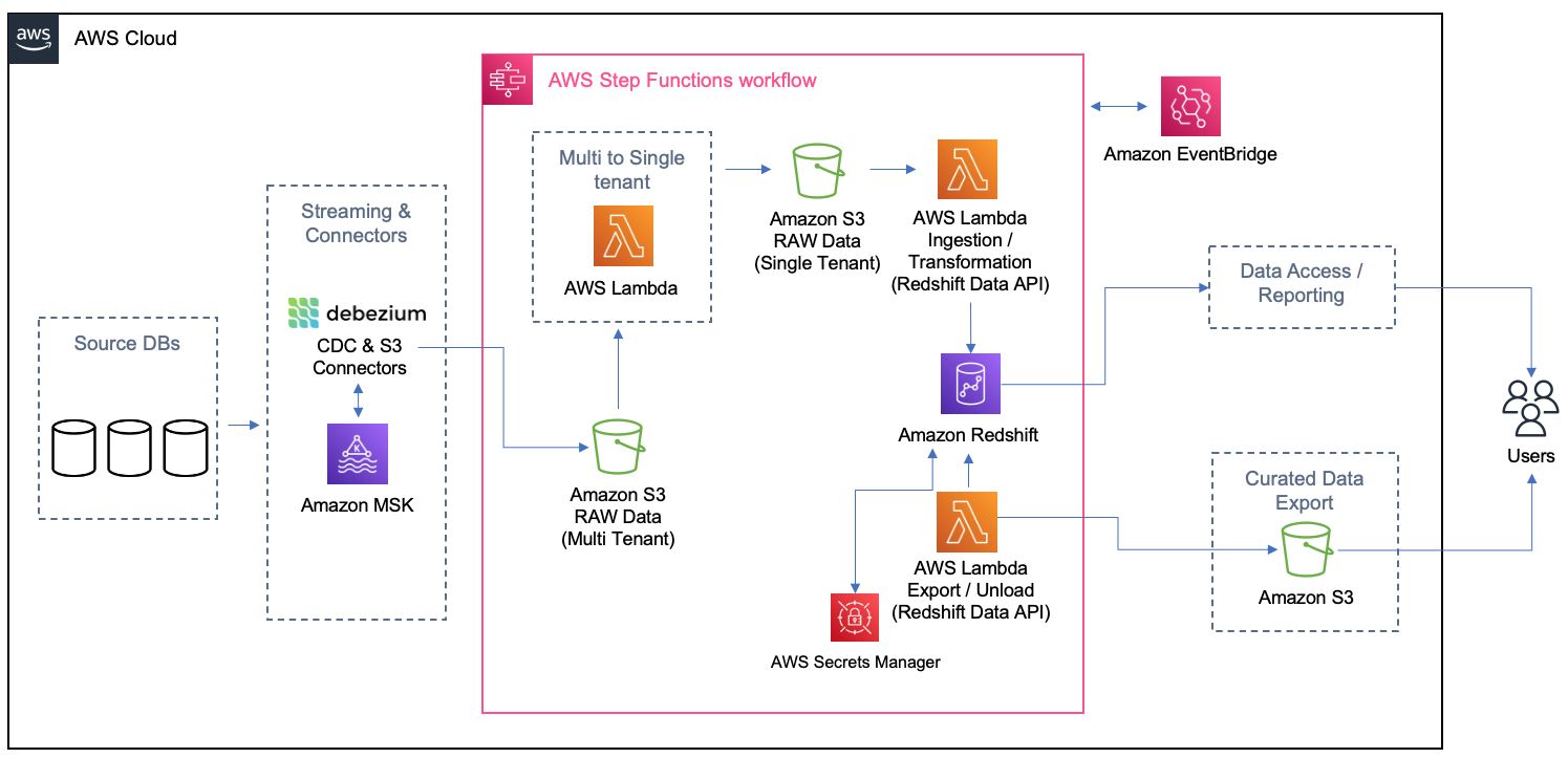
  Parag Doshi is Vice President of Engineering at Tricentis, where he continues to lead towards the vision of Innovation at the Speed of Imagination. He brings innovation to market by building world-class quality engineering SaaS such as qTest, the flagship test management product, and a new capability called Tricentis Analytics, which unlocks software development lifecycle insights across all types of testing. Prior to Tricentis, Parag was the founder of Anthem’s Cloud Platform Services, where he drove a hybrid cloud and DevSecOps capability and migrated 100 mission-critical applications. He enabled Anthem to build a new pharmacy benefits management business in AWS, resulting in $800 million in total operating gain for Anthem in 2020 per Forbes and CNBC. He also held posts at Hewlett-Packard, having multiple roles including Chief Technologist and head of architecture for DXC’s Virtual Private Cloud, and CTO for HP’s Application Services in the Americas region.

Guru Havanur serves as a Principal, Big Data Engineering and Analytics team in Tricentis. Guru is responsible for data, analytics, development, integration with other products, security, and compliance activities. He strives to work with other Tricentis products and customers to improve data sharing, data quality, data integrity, and data compliance through the modern big data platform. With over 20 years of experience in data warehousing, a variety of databases, integration, architecture, and management, he thrives for excellence.

Simon Guindon is an Architect at Tricentis. He has expertise in large-scale distributed systems and database consistency models, and works with teams in Tricentis around the world on scalability and high availability. You can follow his Twitter @simongui.

Ricardo Serafim is a Senior AWS Data Lab Solutions Architect. With a focus on data pipelines, data lakes, and data warehouses, Ricardo helps customers create an end-to-end architecture and test an MVP as part of their path to production. Outside of work, Ricardo loves to travel with his family and watch soccer games, mainly from the “Timão” Sport Club Corinthians Paulista.

How SikSin improved customer engagement with AWS Data Lab and Amazon Personalize

Post Syndicated from Byungjun Choi original https://aws.amazon.com/blogs/big-data/how-siksin-improved-customer-engagement-with-aws-data-lab-and-amazon-personalize/

This post is co-written with Byungjun Choi and Sangha Yang from SikSin.

SikSin is a technology platform connecting customers with restaurant partners serving their multiple needs. Customers use the SikSin platform to search and discover restaurants, read and write reviews, and view photos. From the restaurateurs’ perspective, SikSin enables restaurant partners to engage and acquire customers in order to grow their business. SikSin has a partnership with 850 corporate companies and more than 50,000 restaurants. They issue restaurant e-vouchers to more than 220,000 members, including individuals as well as corporate members. The SikSin platform receives more than 3 million users in a month. SikSin was listed in the top 100 of the Financial Times’s Asia-Pacific region’s high-growth companies in 2022.

SikSin was looking to deliver improved customer experiences and increase customer engagement. SikSin confronted two business challenges:

  • Customer engagement – SikSin maintains data on more than 750,000 restaurants and has more than 4,000 restaurant articles (and growing). SikSin was looking for a personalized and customized approach to provide restaurant recommendations for their customers and get them engaged with the content, thereby providing a personalized customer experience.
  • Data analysis activities – The SikSin Food Service team experienced difficulties in regards to report generation due to scattered data across multiple systems. The team previously had to submit a request to the IT team and then wait for answers that might be outdated. For the IT team, they needed to manually pull data out of files, databases, and applications, and then combine them upon every request, which is a time-consuming activity. The SikSin Food Service team wanted to view web analytics log data by multiple dimensions, such as customer profiles and places. Examples include page view, conversion rate, and channels.

To overcome these two challenges, SikSin participated in the AWS Data Lab program to assist them in building a prototype solution. The AWS Data Lab offers accelerated, joint-engineering engagements between customers and AWS technical resources to create tangible deliverables that accelerate data and analytics modernization initiatives. The Build Lab is a 2–5-day intensive build with a technical customer team.

In this post, we share how SikSin built the basis for accelerating their data project with the help of the Data Lab and Amazon Personalize.

Use cases

The Data Lab team and SikSin team had three consecutive meetings to discuss business and technical requirements, and decided to work on two uses cases to resolve their two business challenges:

  • Build personalized recommendations – SikSin wanted to deploy a machine learning (ML) model to produce personalized content on the landing page of the platform, particularly restaurants and restaurant articles. The success criteria was to increase the number of page views per session and membership subscription, reduce their bounce rate, and ultimately engage more visitors and members in SikSin’s contents.
  • Establish self-service analytics – SikSin’s business users wanted to reduce time to insight by making data more accessible while removing the reliance on the IT team by giving business users the ability to query data. The key was to consolidate web logs from BigQuery and operational business data from Amazon Relational Data Service (Amazon RDS) into a single place and analyze data whenever they need.

Solution overview

The following architecture depicts what the SikSin team built in the 4-day Build Lab. There are two parts in the solution to address SikSin’s business and technical requirements. The first part (1–8) is for building personalized recommendations, and the second part (A–D) is for establishing self-service analytics.

SikSin Solution Architecture

SikSin deployed an ML model to produce personalized content recommendations by using the following AWS services:

  1. AWS Database Migration Service (AWS DMS) helps migrate databases to AWS quickly and securely with minimal downtime. The SikSin team used AWS DMS to perform full load to bring data from the database tables into Amazon Simple Storage Service (Amazon S3) as a target. Amazon S3 is an object storage service offering industry-leading scalability, data availability, security, and performance. An AWS Glue crawler populates the AWS Glue Data Catalog with the data schema definitions (in a landing folder).
  2. An AWS Lambda function checks if any previous files still exist in the landing folder and archives the files into a backup folder, if any.
  3. AWS Glue is a serverless data integration service that makes it easier to discover, prepare, move, and integrate data from multiple sources for analytics, ML, and application development. The SikSin team created AWS Glue Spark extract, transform, and load (ETL) jobs to prepare input datasets for ML models. These datasets are used to train ML models in bulk mode. There are a total of five datasets for training and two datasets for batch inference jobs.
  4. Amazon Personalize allows developers to quickly build and deploy curated recommendations and intelligent user segmentation at scale using ML. Because Amazon Personalize can be tailored to your individual needs, you can deliver the right customer experience at the right time and in the right place. Also, users will select existing ML models (also known as recipes), train models, and run batch inference to make recommendations.
  5. An Amazon Personalize job predicts for each line of input data (restaurants and restaurant articles) and produces ML-generated recommendations in the designated S3 output folder. The recommendation records are surfaced using interaction data, product data, and predictive models. An AWS Glue crawler populates the AWS Glue Data Catalog with the data schema definitions (in an output folder).
  6. The SikSin team applied business logics and filters in an AWS Glue job to prepare the final datasets for recommendations.
  7. AWS Step Functions enables you to build scalable, distributed applications using state machines. The SikSin team used AWS Step Functions Workflow Studio to visually create, run, and debug workflow runs. This workflow is triggered based on a schedule. The process includes data ingestion, cleansing, processing, and all steps defined in Amazon Personalize. This also involves managing run dependencies, scheduling, error-catching, and concurrency in accordance with the logical flow of the pipeline.
  8. Amazon Simple Notification Service (Amazon SNS) sends notifications. The SikSin team used Amazon SNS to send a notification via email and Google Hangouts with a Lambda function as a target.

To establish a self-service analytics environment to enable business users to perform data analysis, SikSin used the following services:

  1. The Google BigQuery Connector for AWS Glue simplifies the process of connecting AWS Glue jobs to extract data from BigQuery. The SikSin team used the connector to extract web analytics logs from BigQuery and load them to an S3 bucket.
  2. AWS Glue DataBrew is a visual data preparation tool that makes it easy for data analysts and data scientists to clean and normalize data to prepare it for analytics and ML. You can choose from over 250 pre-built transformations to automate data preparation tasks, all without the need to write any code. The SikSin Food Service team used it to visually inspect large datasets and shape the data for their data analysis activities. An S3 bucket (in the intermediate folder) contains business operational data such as customers, places, articles, and products, and reference data loaded from AWS DMS and web analytics logs and data by AWS Glue jobs.
  3. An AWS Glue Python shell runs a job to cleanse and join data, and apply business rules to prepare the data for queries. The SikSin team used AWS SDK Pandas, an AWS Professional Service open-source Python initiative, which extends the power of the Pandas library to AWS, connecting DataFrames and AWS data related services. The output files are stored in an Apache Parquet format in a single folder. An AWS Glue crawler populates the data schema definitions (in an output folder) into the AWS Glue Data Catalog.
  4. The SikSin Food Service team used Amazon Athena and Amazon Quicksight to query and visualize the data analysis. Athena is an interactive query service that makes it easy to analyze data in Amazon S3 using standard SQL. QuickSight is an ML-powered business intelligence service built for the cloud.

Business outcomes

The SikSin Food Service team is now able to access the available data for performing data analysis and manipulation operations efficiently, as well as for getting insights on their own. This immediately allows the team as well as other lines of business to understand how customers are interacting with SikSin’s contents and services on the platform and make decisions sooner. For example, with the data output, the Food Service team was able to provide insights and data points for their external stakeholder and customer to initiate a new business idea. Moreover, the team shared, “We anticipate the recommendations and personalized content will increase conversion rates and customer engagement.”

The AWS Data Lab enabled SikSin to review and assess thoroughly what data is actually usable and available. With SikSin’s objective to successfully build a data pipeline for data analytics purposes, the SikSin team came to realize the importance of data cleansing, categorization, and standardization. “Only fruitful analysis and recommendation are possible when data is intact and properly cleansed,” said Byungjun Choi (the Head of SikSin’s Food Service Team). After completing the Data Lab, SikSin completed and set up an internal process that can streamline the data cleansing pipeline.

SikSin was stuck in the research phase of looking for a solution to solve their personalization challenges. The AWS Data Lab enabled the SikSin IT Team to get hands-on with the technology and build a minimum viable product (MVP) to explore how Amazon Personalize would work in their environment with their data. They achieved this via the Data Lab by adopting AWS DMS, AWS Glue, Amazon Personalize, and Step Functions. “Though it is still the early stage of building a prototype, I am very confident with the right enablement provided from AWS that an effective recommendation system can be adopted on production level very soon,” commented Sangha Yang (the Head of SikSin IT Team).

Conclusion

As a result of the 4-day Build Lab, the SikSin team left with a working prototype that is custom fit to their needs, gaining a clear path forward for enabling end-users to gain valuable insights into its data. The Data Lab allowed the SikSin team to accelerate the architectural design and prototype build of this solution by months. Based on the lessons and learnings obtained from Data Lab, SikSin is planning to launch a Global News Content Platform equipped with a recommendation feature in FY23.

As demonstrated by SikSin’s achievements, Amazon Personalize allows developers to quickly build and deploy curated recommendations and intelligent user segmentation at scale using ML. Because Amazon Personalize can be tailored to your individual needs, you can deliver the right customer experience at the right time and in the right place. Whether you want to optimize recommendations, target customers more accurately, maximize your data’s value, or promote items using business rules.

To accelerate your digital transformation with ML, the Data Lab program is available to support you by providing prescriptive architectural guidance on a particular use case, sharing best practices, and removing technical roadblocks. You’ll leave the engagement with an architecture or working prototype that is custom fit to your needs, a path to production, and deeper knowledge of AWS services.

Please contact your AWS Account Manager or Solutions Architect to get started. If you don’t have an AWS Account Manager, please contact Sales.


About the Authors

bdb-2857-BJByungjun Choi is the Head of SikSin Food Service at SikSin.

bdb-2857-SHSangha Yang is the Head of IT team at SinSin.

bdb-2857-youngguYounggu Yun is a Senior Data Lab Architect at AWS. He works with customers around the APAC region to help them achieve business goals and solve technical problems by providing prescriptive architectural guidance, sharing best practices, and building innovative solutions together.

Junwoo Lee is an Account Manager at AWS. He provides technical and business support to help customer resolve their problems and enrich customer journey by introducing local and global programs for his customers.

bdb-2857-jinwooJinwoo Park is a Senior Solutions Architect at AWS. He provides technical support for AWS customers to succeed with their cloud journey. He helps customers build more secure, efficient, and cost-optimized architectures and solutions, and delivers best practices and workshops.

How SOCAR built a streaming data pipeline to process IoT data for real-time analytics and control

Post Syndicated from DoYeun Kim original https://aws.amazon.com/blogs/big-data/how-socar-built-a-streaming-data-pipeline-to-process-iot-data-for-real-time-analytics-and-control/

SOCAR is the leading Korean mobility company with strong competitiveness in car-sharing. SOCAR has become a comprehensive mobility platform in collaboration with Nine2One, an e-bike sharing service, and Modu Company, an online parking platform. Backed by advanced technology and data, SOCAR solves mobility-related social problems, such as parking difficulties and traffic congestion, and changes the car ownership-oriented mobility habits in Korea.

SOCAR is building a new fleet management system to manage the many actions and processes that must occur in order for fleet vehicles to run on time, within budget, and at maximum efficiency. To achieve this, SOCAR is looking to build a highly scalable data platform using AWS services to collect, process, store, and analyze internet of things (IoT) streaming data from various vehicle devices and historical operational data.

This in-car device data, combined with operational data such as car details and reservation details, will provide a foundation for analytics use cases. For example, SOCAR will be able to notify customers if they have forgotten to turn their headlights off or to schedule a service if a battery is running low. Unfortunately, the previous architecture didn’t enable the enrichment of IoT data with operational data and couldn’t support streaming analytics use cases.

AWS Data Lab offers accelerated, joint-engineering engagements between customers and AWS technical resources to create tangible deliverables that accelerate data and analytics modernization initiatives. The Build Lab is a 2–5-day intensive build with a technical customer team.

In this post, we share how SOCAR engaged the Data Lab program to assist them in building a prototype solution to overcome these challenges, and to build the basis for accelerating their data project.

Use case 1: Streaming data analytics and real-time control

SOCAR wanted to utilize IoT data for a new business initiative. A fleet management system, where data comes from IoT devices in the vehicles, is a key input to drive business decisions and derive insights. This data is captured by AWS IoT and sent to Amazon Managed Streaming for Apache Kafka (Amazon MSK). By joining the IoT data to other operational datasets, including reservations, car information, device information, and others, the solution can support a number of functions across SOCAR’s business.

An example of real-time monitoring is when a customer turns off the car engine and closes the car door, but the headlights are still on. By using IoT data related to the car light, door, and engine, a notification is sent to the customer to inform them that the car headlights should be turned off.

Although this real-time control is important, they also want to collect historical data—both raw and curated data—in Amazon Simple Storage Service (Amazon S3) to support historical analytics and visualizations by using Amazon QuickSight.

Use case 2: Detect table schema change

The first challenge SOCAR faced was existing batch ingestion pipelines that were prone to breaking when schema changes occurred in the source systems. Additionally, these pipelines didn’t deliver data in a way that was easy for business analysts to consume. In order to meet the future data volumes and business requirements, they needed a pattern for the automated monitoring of batch pipelines with notification of schema changes and the ability to continue processing.

The second challenge was related to the complexity of the JSON files being ingested. The existing batch pipelines weren’t flattening the five-level nested structure, which made it difficult for business users and analysts to gain business insights without any effort on their end.

Overview of solution

In this solution, we followed the serverless data architecture to establish a data platform for SOCAR. This serverless architecture allowed SOCAR to run data pipelines continuously and scale automatically with no setup cost and without managing servers.

AWS Glue is used for both the streaming and batch data pipelines. Amazon Kinesis Data Analytics is used to deliver streaming data with subsecond latencies. In terms of storage, data is stored in Amazon S3 for historical data analysis, auditing, and backup. However, when frequent reading of the latest snapshot data is required by multiple users and applications concurrently, the data is stored and read from Amazon DynamoDB tables. DynamoDB is a key-value and document database that can support tables of virtually any size with horizontal scaling.

Let’s discuss the components of the solution in detail before walking through the steps of the entire data flow.

Component 1: Processing IoT streaming data with business data

The first data pipeline (see the following diagram) processes IoT streaming data with business data from an Amazon Aurora MySQL-Compatible Edition database.

Whenever a transaction occurs in two tables in the Aurora MySQL database, this transaction is captured as data and then loaded into two MSK topics via AWS Database Management (AWS DMS) tasks. One topic conveys the car information table, and the other topic is for the device information table. This data is loaded into a single DynamoDB table that contains all the attributes (or columns) that exist in the two tables in the Aurora MySQL database, along with a primary key. This single DynamoDB table contains the latest snapshot data from the two DB tables, and is important because it contains the latest information of all the cars and devices for the lookup against the streaming IoT data. If the lookup were done on the database directly with the streaming data, it would impact the production database performance.

When the snapshot is available in DynamoDB, an AWS Glue streaming job runs continuously to collect the IoT data and join it with the latest snapshot data in the DynamoDB table to produce the up-to-date output, which is written into another DynamoDB table.

The up-to-date data in DynamoDB is used for real-time monitoring and control that SOCAR’s Data Analytics team performs for safety maintenance and fleet management. This data is ultimately consumed by a number of apps to perform various business activities, including route optimization, real-time monitoring for oil consumption and temperature, and to identify a driver’s driving pattern, tire wear and defect detection, and real-time car crash notifications.

Component 2: Processing IoT data and visualizing the data in dashboards

The second data pipeline (see the following diagram) batch processes the IoT data and visualizes it in QuickSight dashboards.

There are two data sources. The first is the Aurora MySQL database. The two database tables are exported into Amazon S3 from the Aurora MySQL cluster and registered in the AWS Glue Data Catalog as tables. The second data source is Amazon MSK, which receives streaming data from AWS IoT Core. This requires you to create a secure AWS Glue connection for an Apache Kafka data stream. SOCAR’s MSK cluster requires SASL_SSL as a security protocol (for more information, refer to Authentication and authorization for Apache Kafka APIs). To create an MSK connection in AWS Glue and set up connectivity, we use the following CLI command:

aws glue create-connection —connection-input
'{"Name":"kafka-connection","Description":"kafka connection example",
"ConnectionType":"KAFKA",
"ConnectionProperties":{
"KAFKA_BOOTSTRAP_SERVERS":"<server-ip-addresses>",
"KAFKA_SSL_ENABLED":"true",
// "KAFKA_CUSTOM_CERT": "s3://bucket/prefix/cert.pem",
"KAFKA_SECURITY_PROTOCOL" : "SASL_SSL",
"KAFKA_SKIP_CUSTOM_CERT_VALIDATION":"false",
"KAFKA_SASL_MECHANISM": "SCRAM-SHA-512",
"KAFKA_SASL_SCRAM_USERNAME": "<username>",
"KAFKA_SASL_SCRAM_PASSWORD: "<password>"
},
"PhysicalConnectionRequirements":
{"SubnetId":"subnet-xxx","SecurityGroupIdList":["sg-xxx"],"AvailabilityZone":"us-east-1a"}}'

Component 3: Real-time control

The third data pipeline processes the streaming IoT data in millisecond latency from Amazon MSK to produce the output in DynamoDB, and sends a notification in real time if any records are identified as an outlier based on business rules.

AWS IoT Core provides integrations with Amazon MSK to set up real-time streaming data pipelines. To do so, complete the following steps:

  1. On the AWS IoT Core console, choose Act in the navigation pane.
  2. Choose Rules, and create a new rule.
  3. For Actions, choose Add action and choose Kafka.
  4. Choose the VPC destination if required.
  5. Specify the Kafka topic.
  6. Specify the TLS bootstrap servers of your Amazon MSK cluster.

You can view the bootstrap server URLs in the client information of your MSK cluster details. The AWS IoT rule was created with the Kafka topic as an action to provide data from AWS IoT Core to Kafka topics.

SOCAR used Amazon Kinesis Data Analytics Studio to analyze streaming data in real time and build stream-processing applications using standard SQL and Python. We created one table from the Kafka topic using the following code:

CREATE TABLE table_name (
column_name1 VARCHAR,
column_name2 VARCHAR(100),
column_name3 VARCHAR,
column_name4 as TO_TIMESTAMP (`time_column`, 'EEE MMM dd HH:mm:ss z yyyy'),
 WATERMARK FOR column AS column -INTERVAL '5' SECOND
)
PARTITIONED BY (column_name5)
WITH (
'connector'= 'kafka',
'topic' = 'topic_name',
'properties.bootstrap.servers' = '<bootstrap servers shown in the MSK client info dialog>',
'format' = 'json',
'properties.group.id' = 'testGroup1',
'scan.startup.mode'= 'earliest-offset'
);

Then we applied a query with business logic to identify a particular set of records that need to be alerted. When this data is loaded back into another Kafka topic, AWS Lambda functions trigger the downstream action: either load the data into a DynamoDB table or send an email notification.

Component 4: Flattening the nested structure JSON and monitoring schema changes

The final data pipeline (see the following diagram) processes complex, semi-structured, and nested JSON files.

This step uses an AWS Glue DynamicFrame to flatten the nested structure and then land the output in Amazon S3. After the data is loaded, it’s scanned by an AWS Glue crawler to update the Data Catalog table and detect any changes in the schema.

Data flow: Putting it all together

The following diagram illustrates our complete data flow with each component.

Let’s walk through the steps of each pipeline.

The first data pipeline (in red) processes the IoT streaming data with the Aurora MySQL business data:

  1. AWS DMS is used for ongoing replication to continuously apply source changes to the target with minimal latency. The source includes two tables in the Aurora MySQL database tables (carinfo and deviceinfo), and each is linked to two MSK topics via AWS DMS tasks.
  2. Amazon MSK triggers a Lambda function, so whenever a topic receives data, a Lambda function runs to load data into DynamoDB table.
  3. There is a single DynamoDB table with columns that exist from the carinfo table and the deviceinfo table of the Aurora MySQL database. This table consists of all the data from two tables and stores the latest data by performing an upsert operation.
  4. An AWS Glue job continuously receives the IoT data and joins it with data in the DynamoDB table to produce the output into another DynamoDB target table.
  5. This target table contains the final data, which includes all the device and car status information from the IoT devices as well as metadata from the Aurora MySQL table.

The second data pipeline (in green) batch processes IoT data to use in dashboards and for visualization:

  1. The car and reservation data (in two DB tables) is exported via a SQL command from the Aurora MySQL database with the output data available in an S3 bucket. The folders that contain data are registered as an S3 location for the AWS Glue crawler and become available via the AWS Glue Data Catalog.
  2. The MSK input topic continuously receives data from AWS IoT. Each car has a number of IoT devices, and each device captures data and sends it to an MSK input topic. The Amazon MSK S3 sink connector is configured to export data from Kafka topics to Amazon S3 in JSON formats. In addition, the S3 connector exports data by guaranteeing exactly-once delivery semantics to consumers of the S3 objects it produces.
  3. The AWS Glue job runs in a daily batch to load the historical IoT data into Amazon S3 and into two tables (refer to step 1) to produce the output data in an Enriched folder in Amazon S3.
  4. Amazon Athena is used to query data from Amazon S3 and make it available as a dataset in QuickSight for visualizing historical data.

The third data pipeline (in blue) processes streaming IoT data from Amazon MSK with millisecond latency to produce the output in DynamoDB and send a notification:

  1. An Amazon Kinesis Data Analytics Studio notebook powered by Apache Zeppelin and Apache Flink is used to build and deploy its output as a Kinesis Data Analytics application. This application loads data from Amazon MSK in real time, and users can apply business logic to select particular events coming from the IoT real-time data, for example, the car engine is off and the doors are closed, but the headlights are still on. The particular event that users want to capture can be sent to another MSK topic (Outlier) via the Kinesis Data Analytics application.
  2. Amazon MSK triggers a Lambda function, so whenever a topic receives data, a Lambda function runs to send an email notification to users that are subscribed to an Amazon Simple Notification Service (Amazon SNS) topic. An email is published using an SNS notification.
  3. The Kinesis Data Analytics application loads data from AWS IoT, applies business logic, and then loads it into another MSK topic (output). Amazon MSK triggers a Lambda function when data is received, which loads data into a DynamoDB Append table.
  4. Amazon Kinesis Data Analytics Studio is used to run SQL commands for ad hoc interactive analysis on streaming data.

The final data pipeline (in yellow) processes complex, semi-structured, and nested JSON files, and sends a notification when a schema evolves.

  1. An AWS Glue job runs and reads the JSON data from Amazon S3 (as a source), applies logic to flatten the nested schema using a DynamicFrame, and pivots out array columns from the flattened frame.
  2. The output is stored in Amazon S3 and is automatically registered to the AWS Glue Data Catalog table.
  3. Whenever there is a new attribute or change in the JSON input data at any level in the nested structure, the new attribute and change are captured in Amazon EventBridge as an event from the AWS Glue Data Catalog. An email notification is published using Amazon SNS.

Conclusion

As a result of the four-day Build Lab, the SOCAR team left with a working prototype that is custom fit to their needs, gaining a clear path to production. The Data Lab allowed the SOCAR team to build a new streaming data pipeline, enrich IoT data with operational data, and enhance the existing data pipeline to process complex nested JSON data. This establishes a baseline architecture to support the new fleet management system beyond the car-sharing business.


About the Authors

DoYeun Kim is the Head of Data Engineering at SOCAR. He is a passionate software engineering professional with 19+ years experience. He leads a team of 10+ engineers who are responsible for the data platform, data warehouse and MLOps engineering, as well as building in-house data products.

SangSu Park is a Lead Data Architect in SOCAR’s cloud DB team. His passion is to keep learning, embrace challenges, and strive for mutual growth through communication. He loves to travel in search of new cities and places.

YoungMin Park is a Lead Architect in SOCAR’s cloud infrastructure team. His philosophy in life is-whatever it may be-to challenge, fail, learn, and share such experiences to build a better tomorrow for the world. He enjoys building expertise in various fields and basketball.

Younggu Yun is a Senior Data Lab Architect at AWS. He works with customers around the APAC region to help them achieve business goals and solve technical problems by providing prescriptive architectural guidance, sharing best practices, and building innovative solutions together. In his free time, his son and he are obsessed with Lego blocks to build creative models.

Vicky Falconer leads the AWS Data Lab program across APAC, offering accelerated joint engineering engagements between teams of customer builders and AWS technical resources to create tangible deliverables that accelerate data analytics modernization and machine learning initiatives.

How a blockchain startup built a prototype solution to solve the need of analytics for decentralized applications with AWS Data Lab

Post Syndicated from Dr. Quan Hoang Nguyen original https://aws.amazon.com/blogs/big-data/how-a-blockchain-startup-built-a-prototype-solution-to-solve-the-need-of-analytics-for-decentralized-applications-with-aws-data-lab/

This post is co-written with Dr. Quan Hoang Nguyen, CTO at Fantom Foundation.

Here at Fantom Foundation (Fantom), we have developed a high performance, highly scalable, and secure smart contract platform. It’s designed to overcome limitations of the previous generation of blockchain platforms. The Fantom platform is permissionless, decentralized, and open source. The majority of decentralized applications (dApps) hosted on the Fantom platform lack an analytics page that provides information to the users. Therefore, we would like to build a data platform that supports a web interface that will be made public. This will allow users to search for a smart contract address. The application then displays key metrics for that smart contract. Such an analytics platform can give insights and trends for applications deployed on the platform to the users, while the developers can continue to focus on improving their dApps.

AWS Data Lab offers accelerated, joint-engineering engagements between customers and AWS technical resources to create tangible deliverables that accelerate data and analytics modernization initiatives. Data Lab has three offerings: the Build Lab, the Design Lab, and a Resident Architect. The Build Lab is a 2–5 day intensive build with a technical customer team. The Design Lab is a half-day to 2-day engagement for customers who need a real-world architecture recommendation based on AWS expertise, but aren’t yet ready to build. Both engagements are hosted either online or at an in-person AWS Data Lab hub. The Resident Architect provides AWS customers with technical and strategic guidance in refining, implementing, and accelerating their data strategy and solutions over a 6-month engagement.

In this post, we share the experience of our engagement with AWS Data Lab to accelerate the initiative of developing a data pipeline from an idea to a solution. Over 4 weeks, we conducted technical design sessions, reviewed architecture options, and built the proof of concept data pipeline.

Use case review

The process started with us engaging with our AWS Account team to submit a nomination for the data lab. This followed by a call with the AWS Data Lab team to assess the suitability of requirements against the program. After the Build Lab was scheduled, an AWS Data Lab Architect engaged with us to conduct a series of pre-lab calls to finalize the scope, architecture, goals, and success criteria for the lab. The scope was to design a data pipeline that would ingest and store historical and real-time on-chain transactions data, and build a data pipeline to generate key metrics. Once ingested, data should be transformed, stored, and exposed via REST-based APIs and consumed by a web UI to display key metrics. For this Build Lab, we choose to ingest data for Spooky, which is a decentralized exchange (DEX) deployed on the Fantom platform and had the largest Total Value Locked (TVL) at that time. Key metrics such number of wallets that have interacted with the dApp over time, number of tokens and their value exchanged for the dApp over time, and number of transactions for the dApp over time were selected to visualize through a web-based UI.

We explored several architecture options and picked one for the lab that aligned closely with our end goal. The total historical data for the selected smart contract was approximately 1 GB since deployment of dApp on the Fantom platform. We used FTMScan, which allows us to explore and search on the Fantom platform for transactions, to estimate the rate of transfer transactions to be approximately three to four per minute. This allowed us to design an architecture for the lab that can handle this data ingestion rate. We agreed to use an existing application known as the data producer that was developed internally by the Fantom team to ingest on-chain transactions in real time. On checking transactions’ payload size, it was found to not exceed 100 kb for each transaction, which gave us the measure of number of files that will be created once ingested through the data producer application. A decision was made to ingest the past 45 days of historic transactions to populate the platform with enough data to visualize key metrics. Because the feature of backdating exists within the data producer application, we agreed to use that. The Data Lab Architect also advised us to consider using AWS Database Migration Service (AWS DMS) to ingest historic transactions data post lab. As a last step, we decided to build a React-based webpage with Material-UI that allows users to enter a smart contract address and choose the time interval, and the app fetches the necessary data to show the metrics value.

Solution overview

We collectively agreed to incorporate the following design principles for the data lab architecture:

  • Simplified data pipelines
  • Decentralized data architecture
  • Minimize latency as much as possible

The following diagram illustrates the architecture that we built in the lab.

We collectively defined the following success criteria for the Build Lab:

  • End-to-end data streaming pipeline to ingest on-chain transactions
  • Historical data ingestion of the selected smart contract
  • Data storage and processing of on-chain transactions
  • REST-based APIs to provide time-based metrics for the three defined use cases
  • A sample web UI to display aggregated metrics for the smart contract

Prior to the Build Lab

As a prerequisite for the lab, we configured the data producer application to use the AWS Software Development Kit (AWS SDK) and PUTRecords API operation to send transactions data to an Amazon Simple Storage Service (Amazon S3) bucket. For the Build Lab, we built additional logic within the application to ingest historic transactions data together with real-time transactions data. As a last step, we verified that transactions data was captured and ingested into a test S3 bucket.

AWS services used in the lab

We used the following AWS services as part of the lab:

  • AWS Identity and Access Management (IAM) – We created multiple IAM roles with appropriate trust relationships and necessary permissions that can be used by multiple services to read and write on-chain transactions data and generated logs.
  • Amazon S3 – We created an S3 bucket to store the incoming transactions data as JSON-based files. We created a separate S3 bucket to store incoming transaction data that failed to be transformed and will be reprocessed later.
  • Amazon Kinesis Data Streams – We created a new Kinesis data stream in on-demand mode, which automatically scales based on data ingestion patterns and provides hands-free capacity management. This stream was used by the data producer application to ingest historical and real-time on-chain transactions. We discussed having the ability to manage and predict cost, and therefore were advised to use the provisioned mode when reliable estimates were available for throughput requirements. We were also advised to continue to use on-demand mode until the data traffic patterns were unpredictable.
  • Amazon Kinesis Data Firehose – We created a Firehose delivery stream to transform the incoming data and writes it to the S3 bucket. To minimize latency, we set the delivery stream buffer size to 1 MiB and buffer interval to 60 seconds. This would ensure a file is written to the S3 bucket when either of the two conditions are satisfied regardless of the order. Transactions data written to the S3 bucket was in JSON Lines format.
  • Amazon Simple Queue Service (Amazon SQS) – We set up an SQS queue of the type Standard and an access policy for that SQS queue to allow incoming messages generated from S3 bucket event notifications.
  • Amazon DynamoDB – In order to pick a data store for on-chain transactions, we needed a service that can store transactions payload of unstructured data with varying schemas, provides the ability to cache query results, and is a managed service. We picked DynamoDB for those reasons. We created a single DynamoDB table that holds the incoming transactions data. After analyzing the access query patterns, we decided to use the address field of the smart contract as the partition key and the timestamp field as the sort key. The table was created with auto scaling of read and write capacity modes because the actual usage requirements would be hard to predict at that time.
  • AWS Lambda – We created the following functions:
    • A Python-based Lambda function to perform transformations on the incoming data from the data producer application to flatten the JSON structure, convert the Unix-based epoch timestamp to a date/time value, and convert hex-based string values to a decimal value representing the number of tokens.
    • A second Lambda function to parse incoming SQS queue messages. This message contained values for bucket_name and object_key, which holds the reference to a newly created object within the S3 bucket. The Lambda function logic included parsing of this value to obtain the reference to the S3 object, get the contents of the object, read it into a data frame object using the AWS SDK for pandas (awswrangler) library, convert it into a Pandas data frame object, and use the put_df API call to write a Pandas data frame object as an item into a DynamoDB table. We choose to use Pandas due to familiarity with the library and functions required to perform data transform operations.
    • Three separate Lambda functions that contains the logic to query the DynamoDB table and retrieve items to aggregate and calculate metrics values. This calculated metrics value within the Lambda function was formatted as an HTTP response to expose as REST-based APIs.
  • Amazon API Gateway – We created a REST based API endpoint that uses Lambda proxy integration to pass a smart contract address and time-based interval in minutes as a query string parameter to the backend Lambda function. The response from the Lambda function was a metrics value. We also enabled cross-origin resource sharing (CORS) support within API Gateway to successfully query from the web UI that resides in a different domain.
  • Amazon CloudWatch – We used a Lambda function in-built mechanism to send function metrics to CloudWatch. Lambda functions come with a CloudWatch Logs log group and a log stream for each instance of your function. The Lambda runtime environment sends details of each invocation to the log stream, and relays logs and other output from your function’s code.

Iterative development approach

Across 4 days of the Build Lab, we undertook iterative development. We started by developing the foundational layer and iteratively added extra features through testing and data validation. This allowed us to develop confidence of the solution being built as we tested the output of the metrics through a web-based UI and verified with the actual data. As errors got discovered, we deleted the entire dataset and reran all the jobs to verify results and resolve those errors.

Lab outcomes

In 4 days, we built an end-to-end streaming pipeline ingesting 45 days of historical data and real-time on-chain transactions data for the selected Spooky smart contract. We also developed three REST-based APIs for the selected metrics and a sample web UI that allows users to insert a smart contract address, choose a time frequency, and visualize the metrics values. In a follow-up call, our AWS Data Lab Architect shared post-lab guidance around the next steps required to productionize the solution:

  • Scaling of the proof of concept to handle larger data volumes
  • Security best practices to protect the data while at rest and in transit
  • Best practices for data modeling and storage
  • Building an automated resilience technique to handle failed processing of the transactions data
  • Incorporating high availability and disaster recovery solutions to handle incoming data requests, including adding of the caching layer

Conclusion

Through a short engagement and small team, we accelerated this project from an idea to a solution. This experience gave us the opportunity to explore AWS services and their analytical capabilities in-depth. As a next step, we will continue to take advantage of AWS teams to enhance the solution built during this lab to make it ready for the production deployment.

Learn more about how the AWS Data Lab can help your data and analytics on the cloud journey.


About the Authors

Dr. Quan Hoang Nguyen is currently a CTO at Fantom Foundation. His interests include DLT, blockchain technologies, visual analytics, compiler optimization, and transactional memory. He has experience in R&D at the University of Sydney, IBM, Capital Markets CRC, Smarts – NASDAQ, and National ICT Australia (NICTA).

Ankit Patira is a Data Lab Architect at AWS based in Melbourne, Australia.

How AWS Data Lab helped BMW Financial Services design and build a multi-account modern data architecture

Post Syndicated from Rahul Shaurya original https://aws.amazon.com/blogs/big-data/how-aws-data-lab-helped-bmw-financial-services-design-and-build-a-multi-account-modern-data-architecture/

This post is co-written by Martin Zoellner, Thomas Ehrlich and Veronika Bogusch from BMW Group.

BMW Group and AWS announced a comprehensive strategic collaboration in 2020. The goal of the collaboration is to further accelerate BMW Group’s pace of innovation by placing data and analytics at the center of its decision-making. A key element of the collaboration is the further development of the Cloud Data Hub (CDH) of BMW Group. This is the central platform for managing company-wide data and data solutions in the cloud. At the AWS re:Invent 2019 session, BMW and AWS demonstrated the new Cloud Data Hub platform by outlining different archetypes of data platforms and then walking through the journey of building BMW Group’s Cloud Data Hub. To learn more about the Cloud Data Hub, refer to BMW Cloud Data Hub: A reference implementation of the modern data architecture on AWS.

As part of this collaboration, BMW Group is migrating hundreds of data sources across several data domains to the Cloud Data Hub. Several of these sources pertain to BMW Financial Services.

In this post, we talk about how the AWS Data Lab is helping BMW Financial Services build a regulatory reporting application for one of the European BMW market using the Cloud Data Hub on AWS.

Solution overview

In the context of regulatory reporting, BMW Financial Services works with critical financial services data that contains personally identifiable information (PII). We need to provide monthly insights on our financial data to one of the European National Regulator, and we also need to be compliant with the Schrems II and GDPR regulations as we process PII data. This requires the PII to be pseudonymized when it’s loaded into the Cloud Data Hub, and it has to be processed further in pseudonymized form. For an overview of pseudonymization process, check out Build a pseudonymization service on AWS to protect sensitive data .

To address these requirements in a precise and efficient way, BMW Financial Services decided to engage with the AWS Data Lab. The AWS Data Lab has two offerings: the Design Lab and the Build Lab.

Design Lab

The Design Lab is a 1-to-2-day engagement for customers who need a real-world architecture recommendation based on AWS expertise, but aren’t ready to build. In the case of BMW Financial Services, before beginning the build phase, it was key to get all the stakeholders in the same room and record all the functional and non-functional requirements introduced by all the different parties that might influence the data platform—from owners of the various data sources to end-users that would use the platform to run analytics and get business insights. Within the scope of the Design Lab, we discussed three use cases:

  • Regulatory reporting – The top priority for BMW Financial Services was the regulatory reporting use case, which involves collecting and calculating data and reports that will be declared to the National Regulator.
  • Local data warehouse – For this use case, we need to calculate and store all key performance indicators (KPIs) and key value indicators (KVIs) that will be defined during the project. The historical data needs to be stored, but we need to apply a pseudonymization process to respect GDPR directives. Moreover, historical data has to be accessed on a daily basis through a tableau visualization tool. Regarding the structure, it would be valuable to define two levels (at minimum): one at the contract level to justify the calculation of all KPIs, and another at an aggregated level to optimize restitutions. Personal data is limited in the application, but a reidentification process must be possible for authorized consumption patterns.
  • Accounting details – This use case is based on the BMW accounting tool IFT, which provides the accounting balance at the contract level from all local market applications. It must run at least once a month. However, if some issues are identified on IFT during closing, we must be able to restart it and erase the previous run. When the month-end closing is complete, this use case has to keep the last accounting balance version generated during the month and store it. In parallel, all accounting balance versions have to be accessible by other applications for queries and be able to retrieve the information for 24 months.

Design Lab Solution Architecture

Based on these requirements, we developed the following architecture during the Design Lab.

This solution contains the following components:

  1. The main data source that hydrates our three use cases is the already available in the Cloud Data Hub. The Cloud Data Hub uses AWS Lake Formation resource links to grant access to the dataset to the consumer accounts.
  2. For standard, periodic ETL (extract, transform, and load) jobs that involve operations such as converting data types, or creating labels based on numerical values or Boolean flags based on a label, we used AWS Glue ETL jobs.
  3. For historical ETL jobs or more complex calculations such as in the account details use case, which may involve huge joins with custom configurations and tuning, we recommended to use Amazon EMR. This gives you the opportunity to control cluster configurations at a fine-grained level.
  4. To store job metadata that enables features such as reprocessing inputs or rerunning failed jobs, we recommended building a data registry. The goal of the data registry is to create a centralized inventory for any data being ingested in the data lake. A schedule-based AWS Lambda function could be triggered to register data landing on the semantic layer of the Cloud Data Hub in a centralized metadata store. We recommended using Amazon DynamoDB for the data registry.
  5. Amazon Simple Storage Service (Amazon S3) serves as the storage mechanism that powers the regulatory reporting use case using the data management framework Apache Hudi. Apache Hudi is useful for our use cases because we need to develop data pipelines where record-level insert, update, upsert, and delete capabilities are desirable. Hudi tables are supported by both Amazon EMR and AWS Glue jobs via the Hudi connector, along with query engines such as Amazon Athena and Amazon Redshift Spectrum.
  6. As part of the data storing process in the regulatory reporting S3 bucket, we can populate the AWS Glue Data Catalog with the required metadata.
  7. Athena provides an ad hoc query environment for interactive analysis of data stored in Amazon S3 using standard SQL. It has an out-of-the-box integration with the AWS Glue Data Catalog.
  8. For the data warehousing use case, we need to first de-normalize data to create a dimensional model that enables optimized analytical queries. For that conversion, we use AWS Glue ETL jobs.
  9. Dimensional data marts in Amazon Redshift enable our dashboard and self-service reporting needs. Data in Amazon Redshift is organized into several subject areas that are aligned with the business needs, and a dimensional model allows for cross-subject area analysis.
  10. As a by-product of creating an Amazon Redshift cluster, we can use Redshift Spectrum to access data in the regulatory reporting bucket of the architecture. It acts as a front to access more granular data without actually loading it in the Amazon Redshift cluster.
  11. The data provided to the Cloud Data Hub contains personal data that is pseudonymized. However, we need our pseudonymized columns to be re-personalized when visualizing them on Tableau or when generating CSV reports. Both Athena and Amazon Redshift support Lambda UDFs, which can be used to access Cloud Data Hub PII APIs to re-personalize the pseudonymized columns before presenting them to end-users.
  12. Both Athena and Amazon Redshift can be accessed via JDBC (Java Database Connectivity) to provide access to data consumers.
  13. We can use a Python shell job in AWS Glue to run a query against either of our analytics solutions, convert the results to the required CSV format, and store them to a BMW secured folder.
  14. Any business intelligence (BI) tool deployed on premises can connect to both Athena and Amazon Redshift and use their query engines to perform any heavy computation before it receives the final data to fuel its dashboards.
  15. For the data pipeline orchestration, we recommended using AWS Step Functions because of its low-code development experience and its full integration with all the other components discussed.

With the preceding architecture as our long-term target state, we concluded the Design Lab and decided to return for a Build Lab to accelerate solution development.

Preparing for Build Lab

The typical preparation of a Build Lab that follows a Design Lab involves identifying a few examples of common use case patterns, typically the more complex ones. To maximize the success in the Build Lab, we reduce the long-term target architecture to a subset of components that addresses those examples and can be implemented within a 3-to-5-day intense sprint.

For a successful Build Lab, we also need to identify and resolve any external dependencies, such as network connectivity to data sources and targets. If that isn’t feasible, then we find meaningful ways to mock them. For instance, to make the prototype closer to what the production environment would look like, we decided to use separate AWS accounts for each use case, based on the existing team structure of BMW, and use a consumer S3 bucket instead of BMW network-attached storage (NAS).

Build Lab

The BMW team set aside 4 days for their Build Lab. During that time, their dedicated Data Lab Architect worked alongside the team, helping them to build the following prototype architecture.

Build Lab Solution

This solution includes the following components:

  1. The first step was to synchronize the AWS Glue Data Catalog of the Cloud Data Hub and regulatory reporting accounts.
  2. AWS Glue jobs running on the regulatory reporting account had access to the data in the Cloud Data Hub resource accounts. During the Build Lab, the BMW team implemented ETL jobs for six tables, addressing insert, update, and delete record requirements using Hudi.
  3. The result of the ETL jobs is stored in the data lake layer stored in the regulatory reporting S3 bucket as Hudi tables that are catalogued in the AWS Glue Data Catalog and can be consumed by multiple AWS services. The bucket is encrypted using AWS Key Management Service (AWS KMS).
  4. Athena is used to run exploratory queries on the data lake.
  5. To demonstrate the cross-account consumption pattern, we created an Amazon Redshift cluster on it, created external tables from the Data Catalog, and used Redshift Spectrum to query the data. To enable cross-account connectivity between the subnet group of the Data Catalog of the regulatory reporting account and the subnet group of the Amazon Redshift cluster on the local data warehouse account, we had to enable VPC peering. To accelerate and optimize the implementation of these configurations during the Build Lab, we received support from an AWS networking subject matter expert, who ran a valuable session, during which the BMW team understood the networking details of the architecture.
  6. For data consumption, the BMW team implemented an AWS Glue Python shell job that connected to Amazon Redshift or Athena using a JDBC connection, ran a query, and stored the results in the reporting bucket as a CSV file, which would later be accessible by the end-users.
  7. End-users can also directly connect to both Athena and Amazon Redshift using a JDBC connection.
  8. We decided to orchestrate the AWS Glue ETL jobs using AWS Glue Workflows. We used the resulting workflow for the end-of-lab demo.

With that, we completed all the goals we had set up and concluded the 4-day Build Lab.

Conclusion

In this post, we walked you through the journey the BMW Financial Services team took with the AWS Data Lab team to participate in a Design Lab to identify a best-fit architecture for their use cases, and the subsequent Build Lab to implement prototypes for regulatory reporting in one of the European BMW market.

To learn more about how AWS Data Lab can help you turn your ideas into solutions, visit AWS Data Lab.

Special thanks to everyone who contributed to the success of the Design and Build Lab: Lionel Mbenda, Mario Robert Tutunea, Marius Abalarus, Maria Dejoie.


About the authors

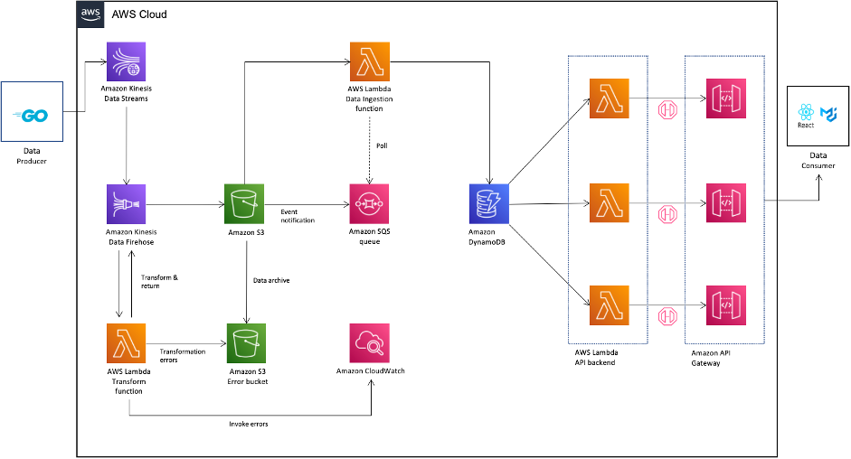
Martin Zoellner is an IT Specialist at BMW Group. His role in the project is Subject Matter Expert for DevOps and ETL/SW Architecture.

Thomas Ehrlich is the functional maintenance manager of Regulatory Reporting application in one of the European BMW market.

Veronika Bogusch is an IT Specialist at BMW. She initiated the rebuild of the Financial Services Batch Integration Layer via the Cloud Data Hub. The ingested data assets are the base for the Regulatory Reporting use case described in this article.

George Komninos is a solutions architect for the Amazon Web Services (AWS) Data Lab. He helps customers convert their ideas to a production-ready data product. Before AWS, he spent three years at Alexa Information domain as a data engineer. Outside of work, George is a football fan and supports the greatest team in the world, Olympiacos Piraeus.

Rahul Shaurya is a Senior Big Data Architect with AWS Professional Services. He helps and works closely with customers building data platforms and analytical applications on AWS. Outside of work, Rahul loves taking long walks with his dog Barney.

Introducing Embedded Analytics Data Lab to accelerate integration of Amazon QuickSight analytics into applications

Post Syndicated from Romit Girdhar original https://aws.amazon.com/blogs/big-data/introducing-embedded-analytics-data-lab-to-accelerate-integration-of-amazon-quicksight-analytics-into-applications/

We are excited to announce Embedded Analytics Data Lab (EADL), a no-cost collaborative engagement that helps engineering and development teams cut down time required to launch applications with embedded analytics from Amazon QuickSight in production by providing hands-on guidance and architectural best practices.

Embedding rich analytics such as interactive visuals and dashboards directly into applications allows developers to create differentiated, analytics-driven experiences that enables end-users to make more informed decisions. QuickSight is a cloud-native, serverless business intelligence (BI) service that allows developers from enterprises and independent software vendors (ISVs) to incorporate powerful BI capabilities such as interactive visualizations, dashboards, and machine learning (ML)-powered natural language query (NLQ) using Amazon QuickSight Q into their applications and web portals, delivering insights to end-users where they are.

AWS Data Lab is an AWS offering that offers accelerated, joint engineering engagements between customers and AWS technical resources to create tangible deliverables that accelerate data, analytics, AI/ML, serverless, and containers modernization initiatives.

Today, with the new EADL offering, we’re bringing together the breadth of QuickSight’s embedding capabilities with proven expertise from AWS Data Lab. With EADL, AWS customers can request a hands-on session to prototype embedded analytics solutions, build custom architectures, and implement best practices with QuickSight-specialist Data Lab Solutions Architects. The output from this engagement is a customized solution that is specific to customer requirements, built using their data, in their AWS account, while providing hands-on learning to the engineering teams attending the lab. EADL engagements accelerate time from ideation to proof of concept to production by months, through tailored guidance while using resources across AWS teams to accelerate the rollout of embedded analytics features powered by QuickSight.

“We’re excited to announce the launch of the Embedded Analytics Data Lab that enables customers and ISVs to accelerate their embedded analytics offering using Amazon QuickSight. With Amazon QuickSight’s embedded analytics capabilities, AWS customers can integrate rich visuals and dashboards into their applications to scale to 100,000s of end-users, differentiating their user experiences—without any servers or infrastructure management. Embedded Analytics Data Lab helps demonstrate this business value in a matter of days by accelerating the QuickSight embedded journey for development teams.”

– Tracy Daugherty, General Manager, Amazon QuickSight.

Customers in EADL work closely with assigned AWS Data Lab Solutions Architect, solidifying the architecture design for their embedded analytics solution, including designing any data model and data pipeline components. The engagement then proceeds to the lab phase, where builders spend 2–4 days with their Solutions Architect, working backward from end goals and building a solution based on the previously defined architecture and real-time guidance from the Solutions Architect and other AWS service experts. Data Lab Solutions Architects also provide implementation guidance on data modeling, setting up multi-tenancy, enabling single sign-on with customers’ identity providers, enabling row- and column-level security, and tracking the health of the QuickSight environment. At lab completion, customers leave with a working prototype of their embedded analytics solution, built by their own builders in their AWS accounts that meet their requirements and specs.

Over the last year, we have worked closely with customers to help design and build their embedded analytics solutions. Some of these customers include BriteCore, Carbyne, and KRS.io.

BriteCore is an enterprise-level insurance processing suite that relies on dashboards to provide operational tracking and trend insights to insurance carriers on data points such as insurance claims and losses by agency, policy type, and line of business. To provide a seamless experience for their over 125,000 customers, BriteCore sought to integrate their BI offerings with their core platform and deliver dashboards to customers as embedded visuals. BriteCore’s engineering and reporting and analytics teams engaged the AWS Data Lab to design and validate the best integration approach between QuickSight and their application and to jumpstart building their interactive, embedded QuickSight dashboards.

“AWS Data Lab was pivotal in helping us build out our embedded analytics solution with the AWS suite of analytics services. Within 4 days, we built a working prototype of our multi-tenant solution with the right identity and security policies in place. Engaging with AWS Data Lab to build our solution definitely helped us reduce our time to production. Our customers now have even better insights into their business, and we will be able to deliver a much richer experience.”

– Supreet Oberoi, Senior Vice President of Engineering, BriteCore.

Carbyne is the global leader in contact center solutions, enabling emergency contact centers and selected enterprises to connect with callers on any connected devices via highly secure communication channels without downloading a consumer app. Carbyne worked with AWS Data Lab to explore options for building a low-latency, multi-tenant analytical system that would enable them to generate meaningful insights using QuickSight’s interactive dashboards for call center owners who manage 911 calls. Example insights include 911 call duration ranges, peak time of day for callers, and percentage of abandoned vs. answered calls—all data points that help Carbyne customers measure the effectiveness of their emergency response systems and then provision staff and resources accordingly. These insights were then embedded into their application, enabling a seamless experience for the 911 call center managers.

“This experience with the AWS Data Lab is what it means to be in true partnership. Data Lab’s support and efforts are much appreciated as we push innovative solutions to the public safety industry. I can say confidently that Data Lab’s support will reduce our time to production by weeks, if not months.”

– Alex Dizengof, Founder & CTO, Carbyne, Inc. 

KRS.io is a leader in coalition loyalty marketing connecting thousands of retailers with their customers on an intimate level with rewards programs and loyalty solutions. To truly democratize data, they set out to build a solution that harnesses the power of NQL. In a 1-day workshop with the AWS Data Lab team, KRS.io embedded QuickSight Q into Epiphany and successfully modeled 20 questions for their Profit Central back office accounting system, perpetual inventory, and loyalty datasets.

“In business, speed matters. Working with AWS Data Lab accelerated our timeframe from proof of concept to deployment. I had zero-tolerance for risk and the Data Lab allowed my team to meet my high bar for security and reliability”

– Brian McManus, CTO, KRS.io.

Get started with EADL

Prerequisites required to qualify for this offering are:

  • Valid embedded analytics use case.
  • Ready and accessible data to be used with QuickSight.
  • Available AWS sandbox or development environment to build the prototype. Data sources for QuickSight must be accessible through this sandbox account.
  • Available webpages or assets to be used to embed the QuickSight visuals and dashboards.
  • Full-time participation of at least two builders, including a builder that is comfortable and familiar with the web assets to be used for embedding.

To get started, register now. Once registered, a member of the AWS team will contact you with next steps.


About the Authors

Romit Girdhar manages Technical Product Management & Software Development teams for AWS Data Lab. He focuses on working backwards from customer outcomes to help accelerate their cloud journey. Romit has over a decade of experience working on engineering solutions for and with customers across two major public cloud companies – Amazon and Microsoft.

Kareem Syed-Mohammed is a Product Manager at Amazon QuickSight. He focuses on embedded analytics, APIs, and developer experience. Prior to QuickSight he has been with AWS Marketplace and Amazon retail as a PM. Kareem started his career as a developer and then PM for call center technologies, Local Expert and Ads for Expedia. He worked as a consultant with McKinsey and Company for a short while.

How the Georgia Data Analytics Center built a cloud analytics solution from scratch with the AWS Data Lab

Post Syndicated from Kanti Chalasani original https://aws.amazon.com/blogs/big-data/how-the-georgia-data-analytics-center-built-a-cloud-analytics-solution-from-scratch-with-the-aws-data-lab/

This is a guest post by Kanti Chalasani, Division Director at Georgia Data Analytics Center (GDAC). GDAC is housed within the Georgia Office of Planning and Budget to facilitate governed data sharing between various state agencies and departments.

The Office of Planning and Budget (OPB) established the Georgia Data Analytics Center (GDAC) with the intent to provide data accountability and transparency in Georgia. GDAC strives to support the state’s government agencies, academic institutions, researchers, and taxpayers with their data needs. Georgia’s modern data analytics center will help to securely harvest, integrate, anonymize, and aggregate data.

In this post, we share how GDAC created an analytics platform from scratch using AWS services and how GDAC collaborated with the AWS Data Lab to accelerate this project from design to build in record time. The pre-planning sessions, technical immersions, pre-build sessions, and post-build sessions helped us focus on our objectives and tangible deliverables. We built a prototype with a modern data architecture and quickly ingested additional data into the data lake and the data warehouse. The purpose-built data and analytics services allowed us to quickly ingest additional data and deliver data analytics dashboards. It was extremely rewarding to officially release the GDAC public website within only 4 months.

A combination of clear direction from OPB executive stakeholders, input from the knowledgeable and driven AWS team, and the GDAC team’s drive and commitment to learning played a huge role in this success story. GDAC’s partner agencies helped tremendously through timely data delivery, data validation, and review.

We had a two-tiered engagement with the AWS Data Lab. In the first tier, we participated in a Design Lab to discuss our near-to-long-term requirements and create a best-fit architecture. We discussed the pros and cons of various services that can help us meet those requirements. We also had meaningful engagement with AWS subject matter experts from various AWS services to dive deeper into the best practices.

The Design Lab was followed by a Build Lab, where we took a smaller cross section of the bigger architecture and implemented a prototype in 4 days. During the Build Lab, we worked in GDAC AWS accounts, using GDAC data and GDAC resources. This not only helped us build the prototype, but also helped us gain hands-on experience in building it. This experience also helped us better maintain the product after we went live. We were able to continually build on this hands-on experience and share the knowledge with other agencies in Georgia.

Our Design and Build Lab experiences are detailed below.

Step 1: Design Lab

We wanted to stand up a platform that can meet the data and analytics needs for the Georgia Data Analytics Center (GDAC) and potentially serve as a gold standard for other government agencies in Georgia. Our objective with the AWS Data Design Lab was to come up with an architecture that meets initial data needs and provides ample scope for future expansion, as our user base and data volume increased. We wanted each component of the architecture to scale independently, with tighter controls on data access. Our objective was to enable easy exploration of data with faster response times using Tableau data analytics as well as build data capital for Georgia. This would allow us to empower our policymakers to make data-driven decisions in a timely manner and allow State agencies to share data and definitions within and across agencies through data governance. We also stressed on data security, classification, obfuscation, auditing, monitoring, logging, and compliance needs. We wanted to use purpose-built tools meant for specialized objectives.

Over the course of the 2-day Design Lab, we defined our overall architecture and picked a scaled-down version to explore. The following diagram illustrates the architecture of our prototype.

The architecture contains the following key components:

  • Amazon Simple Storage Service (Amazon S3) for raw data landing and curated data staging.
  • AWS Glue for extract, transform, and load (ETL) jobs to move data from the Amazon S3 landing zone to Amazon S3 curated zone in optimal format and layout. We used an AWS Glue crawler to update the AWS Glue Data Catalog.
  • AWS Step Functions for AWS Glue job orchestration.
  • Amazon Athena as a powerful tool for a quick and extensive SQL data analysis and to build a logical layer on the landing zone.
  • Amazon Redshift to create a federated data warehouse with conformed dimensions and star schemas for consumption by Tableau data analytics.

Step 2: Pre-Build Lab

We started with planning sessions to build foundational components of our infrastructure: AWS accounts, Amazon Elastic Compute Cloud (Amazon EC2) instances, an Amazon Redshift cluster, a virtual private cloud (VPC), route tables, security groups, encryption keys, access rules, internet gateways, a bastion host, and more. Additionally, we set up AWS Identity and Access Management (IAM) roles and policies, AWS Glue connections, dev endpoints, and notebooks. Files were ingested via secure FTP, or from a database to Amazon S3 using AWS Command Line Interface (AWS CLI). We crawled Amazon S3 via AWS Glue crawlers to build Data Catalog schemas and tables for quick SQL access in Athena.

The GDAC team participated in Immersion Days for training in AWS Glue, AWS Lake Formation, and Amazon Redshift in preparation for the Build Lab.

We defined the following as the success criteria for the Build Lab:

  • Create ETL pipelines from source (Amazon S3 raw) to target (Amazon Redshift). These ETL pipelines should create and load dimensions and facts in Amazon Redshift.
  • Have a mechanism to test the accuracy of the data loaded through our pipelines.
  • Set up Amazon Redshift in a private subnet of a VPC, with appropriate users and roles identified.
  • Connect from AWS Glue to Amazon S3 to Amazon Redshift without going over the internet.
  • Set up row-level filtering in Amazon Redshift based on user login.
  • Data pipelines orchestration using Step Functions.
  • Build and publish Tableau analytics with connections to our star schema in Amazon Redshift.
  • Automate the deployment using AWS CloudFormation.
  • Set up column-level security for the data in Amazon S3 using Lake Formation. This allows for differential access to data based on user roles to users using both Athena and Amazon Redshift Spectrum.

Step 3: Four-day Build Lab

Following a series of implementation sessions with our architect, we formed the GDAC data lake and organized downstream data pulls for the data warehouse with governed data access. Data was ingested in the raw data landing lake and then curated into a staging lake, where data was compressed and partitioned in Parquet format.

It was empowering for us to build PySpark Extract Transform Loads (ETL) AWS Glue jobs with our meticulous AWS Data Lab architect. We built reusable glue jobs for the data ingestion and curation using the code snippets provided. The days were rigorous and long, but we were thrilled to see our centralized data repository come into fruition so rapidly. Cataloging data and using Athena queries proved to be a fast and cost-effective way for data exploration and data wrangling.

The serverless orchestration with Step Functions allowed us to put AWS Glue jobs into a simple readable data workflow. We spent time designing for performance and partitioning data to minimize cost and increase efficiency.

Database access from Tableau and SQL Workbench/J were set up for my team. Our excitement only grew as we began building data analytics and dashboards using our dimensional data models.

Step 4: Post-Build Lab

During our post-Build Lab session, we closed several loose ends and built additional AWS Glue jobs for initial and historic loads and append vs. overwrite strategies. These strategies were picked based on the nature of the data in various tables. We returned for a second Build Lab to work on building data migration tasks from Oracle Database via VPC peering, file processing using AWS Glue DataBrew, and AWS CloudFormation for automated AWS Glue job generation. If you have a team of 4–8 builders looking for a fast and easy foundation for a complete data analytics system, I would highly recommend the AWS Data Lab.

Conclusion

All in all, with a very small team we were able to set up a sustainable framework on AWS infrastructure with elastic scaling to handle future capacity without compromising quality. With this framework in place, we are moving rapidly with new data feeds. This would not have been possible without the assistance of the AWS Data Lab team throughout the project lifecycle. With this quick win, we decided to move forward and build AWS Control Tower with multiple accounts in our landing zone. We brought in professionals to help set up infrastructure and data compliance guardrails and security policies. We are thrilled to continually improve our cloud infrastructure, services and data engineering processes. This strong initial foundation has paved the pathway to endless data projects in Georgia.


About the Author

Kanti Chalasani serves as the Division Director for the Georgia Data Analytics Center (GDAC) at the Office of Planning and Budget (OPB). Kanti is responsible for GDAC’s data management, analytics, security, compliance, and governance activities. She strives to work with state agencies to improve data sharing, data literacy, and data quality through this modern data engineering platform. With over 26 years of experience in IT management, hands-on data warehousing, and analytics experience, she thrives for excellence.

Vishal Pathak is an AWS Data Lab Solutions Architect. Vishal works with customers on their use cases, architects solutions to solve their business problems, and helps them build scalable prototypes. Prior to his journey with AWS, Vishal helped customers implement BI, data warehousing, and data lake projects in the US and Australia.

Design and build a Data Vault model in Amazon Redshift from a transactional database

Post Syndicated from George Komninos original https://aws.amazon.com/blogs/big-data/design-and-build-a-data-vault-model-in-amazon-redshift-from-a-transactional-database/

Building a highly performant data model for an enterprise data warehouse (EDW) has historically involved significant design, development, administration, and operational effort. Furthermore, the data model must be agile and adaptable to change while handling the largest volumes of data efficiently.

Data Vault is a methodology for delivering project design and implementation to accelerate the build of data warehouse projects. Within the overall methodology, the Data Vault 2.0 data modeling standards are popular and widely used within the industry because they emphasize the business keys and their associations within the delivery of business processes. Data Vault facilitates the rapid build of data models via the following:

  • Pattern-based entities each with a well-defined purpose
  • Data silos are removed because data is represented in source system independent structures
  • Data can be loaded in parallel with minimum dependencies
  • Historized data is stored at its lowest level of granularity
  • Flexible business rules can be applied independently of the loading of the data
  • New data sources can be added with no impact on the existing model.

We always recommend working backwards from the business requirements to choose the most suitable data modelling pattern to use; there are times where Data Vault will not be the best choice for your enterprise data warehouse and another modelling pattern will be more suitable.

In this post, we demonstrate how to implement a Data Vault model in Amazon Redshift and query it efficiently by using the latest Amazon Redshift features, such as separation of compute from storage, seamless data sharing, automatic table optimizations, and materialized views.

Data Vault data modeling overview

A data warehouse platform built using Data Vault typically has the following architecture:

The architecture consists of four layers:

  • Staging – Contains a copy of the latest changes to data from the source systems. This layer doesn’t hold history and, during its population, you can apply several transformations to the staged data, including data type changes or resizing, character set conversion, and the addition of meta-data columns to support later processing.
  • Raw Data Vault – Holds the historized copy of all of the data from multiple source systems. No filters or business transformations have occurred at this point except for storing the data in source-system independent targets.
  • Business Data Vault – An optional delivery, but is very often built. It contains business calculations and de-normalizations with the sole purpose of improving the speed and simplicity of access within the consumption layer, which is called the Information Mart layer.
  • Information Mart Layer – Where data is most commonly accessed by consumers, for example reporting dashboards or extracts. You can build multiple marts from the one Data Vault Integration Layer, and the most common data modeling choice for these marts is Star/Kimball schemas.

Convert a Third Normal Form transactional schema to a Data Vault schema

The following entity relationship diagram is a standard implementation of a transactional model that a sports ticket selling service could use:

The main entities within the schema are sporting events, customers, and tickets. A customer is a person, and a person can purchase one or multiple tickets for a sporting event. This business event is captured by the Ticket Purchase History intersection entity above. Finally, a sporting event has many tickets available to purchase and is staged within a single city.

To convert this source model to a Data Vault model, we start to identify the business keys, their descriptive attributes, and the business transactions. The three main entity types in the Raw Data Vault model are as follows:

  • Hubs – A collection of Business Keys discovered for each business entity.
  • Links – Business transactions within the process being modelled. This is always between two or more business keys (hubs) and recorded at a point in time.
  • Satellites – Historized reference data about either the business key (Hub) or business transaction (link).

The following example solution represents some of the sporting event entities when converted into the preceeding Raw Data Vault objects.

Hub entities

The hub is the definitive list of business keys loaded into the Raw Data Vault layer from all of the source systems. A business key is used to uniquely identify a business entity and is never duplicated. In our example, the source system has assigned a surrogate key field called Id to represent the Business Key, so this is stored in a column on the Hub called sport_event_id. Some common additional columns on hubs include the Load DateTimeStamp which records the date and time the business key was first discovered, and the Record Source which records the name of the source system where this business key was first loaded. Although, you don’t have to create a surrogate type (hash or sequence) for the primary key column, it is very common in Data Vault to hash the business key, so our example does this. Amazon Redshift supports multiple cryptographic hash functions like MD5, FNV, SHA1, and SHA2, which you can choose to generate your primary key column. See the following code :

create table raw_data_vault.hub_sport_event 
(
  sport_event_pk  varchar(32) not null     
 ,sport_event_id  integer     not null
 ,load_dts        timestamp   not null       
 ,record_source   varchar(10) not null      
);

Note the following:

  • The preceeding code assumes the MD5 hashing algorithm is used. If using FNV_HASH, the datatype will be Bigint.
  • The Id column is the business key from the source feed. It’s passed into the hashing function for the _PK column.
  • In our example, there is only a single value for the business key. If a compound key is required, then more than one column can be added.
  • Load_DTS is populated via the staging schema or extract, transform, and load (ETL) code.
  • Record_Source is populated via the staging schema or ETL code.

Link entities

The link object is the occurrence of two or more business keys undertaking a business transaction, for example purchasing a ticket for a sporting event. Each of the business keys is mastered in their respective hubs, and a primary key is generated for the link comprising all of the business keys (typically separated by a delimiter field like ‘^’). As with hubs, some common additional columns are added to links, including the Load DateTimeStamp which records the date and time the transaction was first discovered, and the Record Source which records the name of the source system where this transaction was first loaded. See the following code:

create table raw_data_vault.lnk_ticket_sport_event 
(
  ticket_sport_event_pk varchar(32)  not null    
 ,ticket_fk             varchar(32)  not null   
 ,sport_event_fk        varchar(32)  not null   
 ,load_dts              timestamp    not null   
 ,record_source         varchar(10)  not null   
);

Note the following:

  • The code assumes that the MD5 hashing algorithm is used. The _PK column is hashed values of concatenated ticket and sporting event business keys from the source data feed, for example MD5(ticket_id||'^'||sporting_event_id)
  • The two _FK columns are foreign keys linked to the primary key of the respective hubs.
  • Load_DTS is populated via the staging schema or ETL code.
  • Record_Source is populated via the staging schema or ETL code.

Satellite entities

The history of data about the hub or link is stored in the satellite object. The Load DateTimeStamp is part of the compound key of the satellite along with the primary key of either the hub or link because data can change over time. There are choices within the Data Vault standards for how to store satellite data from multiple sources. A common approach is to append the name of the feed to the satellite name. This lets a single hub contain reference data from more than one source system, and for new sources to be added without impact to the existing design. See the following code:

create table raw_data_vault.sat_sport_event 
(
  sport_event_pk    varchar(32) not null     
 ,load_dts          timestamp   not null  
 ,sport_type_name   varchar(50)
 ,start_datetime    timestamp
 ,sold_out          boolean     
 ,record_source     varchar(10) not null 
 ,hash_diff         varchar(32) not null 
);

Note the following:

  • The sport_event_pk value is inherited from the hub.
  • The compound key is the sport_event_pk and load_dts columns. This allows history to be maintained.
  • The business attributes are typically optional.
  • Load_DTS is populated via the staging schema or ETL code.
  • Record_Source is populated via the staging schema or ETL code.
  • Hash_Diff is a Data Vault technique to simplify the identification of data changes within satellites. The business attribute values are concatenated and hashed with your algorithm of choice. Then, during the ETL processing, only the two hash values (one on the source record and one on the latest dated satellite record) should be compared.

Converted Data Vault Model

If we take the preceding three Data Vault entity types above, we can convert the source data model into a Data Vault data model as follows:

The Business Data Vault contains business-centric calculations and performance de-normalizations that are read by the Information Marts. Some of the object types that are created in the Business Vault layer include the following:

  • PIT (point in time) tables – You can store data in more than one satellite for a single hub, each with a different Load DateTimeStamp depending on when the data was loaded. A PIT table simplifies access to all of this data by creating a table or materialized view to present a single row with all of the relevant data to hand. The compound key of a PIT table is the primary key from the hub, plus a snapshot date or snapshot date and time for the frequency of the population. Once a day is the most popular, but equally the frequency could be every 15 minutes or once a month.
  • Bridge tables – Similar to PIT tables, bridge tables take the data from more than one link or link satellite and again de-normalize into a single row. This single row view makes accessing complex datasets over multiple tables from the Raw Data Vault much more straightforward and performant. Like a PIT table, the bridge table can be either a table or materialized view.
  • KPI tables – The pre-computed business rules calculate KPIs and store them in dedicated tables.
  • Type 2 tables –You can apply additional processing in the Business Data Vault to calculate Type 2 like time periods because the data in the Raw Data Vault follows an insert only pattern.

The architecture of Amazon Redshift allows flexibility in the design of the Data Vault platform by using the capabilities of the Amazon Redshift RA3 instance type to separate the compute resources from the data storage layer and the seamless ability to share data between different Amazon Redshift clusters. This flexibility allows highly performant and cost-effective Data Vault platforms to be built. For example, the Staging and Raw Data Vault Layers are populated 24-hours-a-day in micro batches by one Amazon Redshift cluster, the Business Data Vault layer can be built one-time-a-day and paused to save costs when completed, and any number of consumer Amazon Redshift clusters can access the results. Depending on the processing complexity of each layer, Amazon Redshift supports independently scaling the compute capacity required at each stage.

All of the underlying tables in Raw Data Vault can be loaded simultaneously. This makes great use of the massively parallel processing architecture in Amazon Redshift. For our business model, it makes sense to create a Business Data Vault layer, which can be read by an Information Mart to perform dimensional analysis on ticket sales. It can give us insights on the top home teams in fan attendance and how that correlates with specific sport locations or cities. Running these queries involves joining multiple tables. It’s important to design an optimal Business Data Vault layer to avoid excessive joins for deriving these insights.

For example, to get the number of tickets per city for June 2021, the SQL looks like the following code:

SELECT name,count(lpt.ticket_fk) as tickets_sold
FROM lnk_person_ticket lpt
  JOIN lnk_ticket_sport_event ltse on lpt.ticket_fk = ltse.ticket_fk
  JOIN lnk_sport_event_location lsel on ltse.sport_event_fk = lsel.sport_event_fk
  JOIN lnk_location_city llc on lsel.location_fk = llc.location_fk
  JOIN sat_city sc on llc.city_fk = sc.city_pk
  JOIN sat_sport_event sse on lsel.sport_event_fk = sse.sport_event_pk
Where start_date between '2021-06-05' and '2021-06-15' group by 1;

We can use the EXPLAIN command for the preceding query to get the Amazon Redshift query plan. The following plan shows that the specified joins require broadcasting data across nodes, since the join conditions are on different keys. This makes the query computationally expensive:

dev=# explain SELECT
  name, count(lpt.ticket_fk) as tickets_sold FROM lnk_person_ticket lpt
  JOIN lnk_ticket_sport_event ltse on lpt.ticket_fk = ltse.ticket_fk
  JOIN lnk_sport_event_location lsel on ltse.sport_event_fk = lsel.sport_event_fk
  JOIN lnk_location_city llc on lsel.location_fk = llc.location_fk
  JOIN sat_city sc on llc.city_fk = sc.city_pk
  JOIN sat_sport_event sse on lsel.sport_event_fk = sse.sport_event_pk
where
  start_date between ‘2021-06-05’
  and ‘2021-06-15’
GROUP BY
  1;
                            QUERY PLAN
----------------------------------------------------------------------
 XN HashAggregate  (cost=96331086541.29..96331086564.36 rows=9226 width=49)
   ->  XN Hash Join DS_BCAST_INNER  (cost=166693605.84..96331086495.16 rows=9226 width=49)
         Hash Cond: ((“outer”.ticket_fk)::text = (“inner”.ticket_fk)::text)
         ->  XN Hash Join DS_BCAST_INNER  (cost=166690878.95..344629685.90 rows=621783 width=49)
               Hash Cond: ((“outer”.sport_event_fk)::text = (“inner”.sport_event_fk)::text)
               ->  XN Seq Scan on lnk_ticket_sport_event ltse  (cost=0.00..147804.35 rows=14780435 width=72)
               ->  XN Hash  (cost=166690878.49..166690878.49 rows=185 width=85)
                     ->  XN Hash Join DS_BCAST_INNER  (cost=49690773.08..166690878.49 rows=185 width=85)
                           Hash Cond: ((“outer”.location_fk)::text = (“inner”.location_fk)::text)
                           ->  XN Hash Join DS_BCAST_INNER  (cost=65.61..79200165.14 rows=179 width=108)
                                 Hash Cond: ((“outer”.sport_event_fk)::text = (“inner”.sport_event_pk)::text)
                                 ->  XN Seq Scan on lnk_sport_event_location lsel  (cost=0.00..43.44 rows=4344 width=72)
                                 ->  XN Hash  (cost=65.16..65.16 rows=180 width=36)
                                       ->  XN Seq Scan on sat_sport_event sse  (cost=0.00..65.16 rows=180 width=36)
                                             Filter: ((start_date <= ‘2021-06-15’::date) AND (start_date >= ‘2021-06-05’::date))
                           ->  XN Hash  (cost=49690707.31..49690707.31 rows=63 width=49)
                                 ->  XN Hash Join DS_BCAST_INNER  (cost=0.78..49690707.31 rows=63 width=49)
                                       Hash Cond: ((“outer”.city_pk)::text = (“inner”.city_fk)::text)
                                       ->  XN Seq Scan on sat_city sc  (cost=0.00..27909.51 rows=2790951 width=49)
                                       ->  XN Hash  (cost=0.62..0.62 rows=62 width=72)
                                             ->  XN Seq Scan on lnk_location_city llc  (cost=0.00..0.62 rows=62 width=72)
         ->  XN Hash  (cost=2181.51..2181.51 rows=218151 width=36)
               ->  XN Seq Scan on lnk_person_ticket lpt  (cost=0.00..2181.51 rows=218151 width=36)
(23 rows)

Let’s discuss the latest Amazon Redshift features that help optimize the performance of these queries on top of a Business Data Vault model.

Use Amazon Redshift features to query the Data Vault

Automatic table optimization

Traditionally, to optimize joins in Amazon Redshift, it’s recommended to use distribution keys and styles to co-locate data in the same nodes, as based on common join predicates. The Raw Data Vault layer has a very well-defined pattern, which is ideal for determining the distribution keys. However, the broad range of SQL queries applicable to the Business Data Vault makes it hard to predict your consumption pattern that would drive your distribution strategy.

Automatic table optimization lets you get the fastest performance quickly without needing to invest time to manually tune and implement table optimizations. Automatic table optimization continuously observes how queries interact with tables, and it uses machine learning (ML) to select the best sort and distribution keys to optimize performance for the cluster’s workload. If Amazon Redshift determines that applying a key will improve cluster performance, then tables are automatically altered within hours without requiring administrator intervention.

Automatic Table Optimization provided following recommendations for the above query to get the number of tickets per city for June 2021. The recommendations suggest modifying the distribution style and sort keys for tables involved in these queries.

dev=# select * from svv_alter_table_recommendations;
   type    | database | table_id | group_id |                                           ddl                                           | auto_eligible
-----------+----------+----------+----------+-----------------------------------------------------------------------------------------+---------------
 diststyle | dev      |   127372 |        0 | ALTER TABLE “public”.“lnk_person_ticket” ALTER DISTSTYLE KEY DISTKEY “ticket_fk”        | f
 sortkey   | dev      |   127421 |       -1 | ALTER TABLE “public”.“lnk_ticket_sport_event” ALTER COMPOUND SORTKEY (“sport_event_fk”) | f
 diststyle | dev      |   127421 |        0 | ALTER TABLE “public”.“lnk_ticket_sport_event” ALTER DISTSTYLE KEY DISTKEY “ticket_fk”   | f
 sortkey   | dev      |   145032 |       -1 | ALTER TABLE “public”.“sat_city” ALTER COMPOUND SORTKEY (“city_pk”)                      | f

After the recommended distribution keys and sort keys were applied by Automatic Table Optimization, the explain plan shows “DS_DIST_NONE” and no data redistribution was required anymore for this query. The data required for the joins was co-located across Amazon Redshift nodes.

QUERY PLAN
----------------------------------------------------------------------
 XN HashAggregate  (cost=344646541.29..344646564.36 rows=9226 width=49)
   ->  XN Hash Join DS_DIST_NONE  (cost=166693605.84..344646495.16 rows=9226 width=49)
         Hash Cond: ((“outer”.ticket_fk)::text = (“inner”.ticket_fk)::text)
         ->  XN Hash Join DS_BCAST_INNER  (cost=166690878.95..344629685.90 rows=621783 width=49)
               Hash Cond: ((“outer”.sport_event_fk)::text = (“inner”.sport_event_fk)::text)
               ->  XN Seq Scan on lnk_ticket_sport_event ltse  (cost=0.00..147804.35 rows=14780435 width=72)
               ->  XN Hash  (cost=166690878.49..166690878.49 rows=185 width=85)
                     ->  XN Hash Join DS_BCAST_INNER  (cost=49690773.08..166690878.49 rows=185 width=85)
                           Hash Cond: ((“outer”.location_fk)::text = (“inner”.location_fk)::text)
                           ->  XN Hash Join DS_BCAST_INNER  (cost=65.61..79200165.14 rows=179 width=108)
                                 Hash Cond: ((“outer”.sport_event_fk)::text = (“inner”.sport_event_pk)::text)
                                 ->  XN Seq Scan on lnk_sport_event_location lsel  (cost=0.00..43.44 rows=4344 width=72)
                                 ->  XN Hash  (cost=65.16..65.16 rows=180 width=36)
                                       ->  XN Seq Scan on sat_sport_event sse  (cost=0.00..65.16 rows=180 width=36)
                                             Filter: ((start_date <= ‘2021-06-15’::date) AND (start_date >= ‘2021-06-05’::date))
                           ->  XN Hash  (cost=49690707.31..49690707.31 rows=63 width=49)
                                 ->  XN Hash Join DS_BCAST_INNER  (cost=0.78..49690707.31 rows=63 width=49)
                                       Hash Cond: ((“outer”.city_pk)::text = (“inner”.city_fk)::text)
                                       ->  XN Seq Scan on sat_city sc  (cost=0.00..27909.51 rows=2790951 width=49)
                                       ->  XN Hash  (cost=0.62..0.62 rows=62 width=72)
                                             ->  XN Seq Scan on lnk_location_city llc  (cost=0.00..0.62 rows=62 width=72)
         ->  XN Hash  (cost=2181.51..2181.51 rows=218151 width=36)
               ->  XN Seq Scan on lnk_person_ticket lpt  (cost=0.00..2181.51 rows=218151 width=36)
(23 rows)

Materialized views in Amazon Redshift

The data analyst responsible for running this analysis benefits significantly by creating a materialized view in the Business Data Vault schema that pre-computes the results of the queries by running the following SQL:

CREATE MATERIALIZED VIEW bridge_city_ticket_aggregation_mv
AUTO REFRESH YES
AS SELECT name, count(lpt.ticket_fk) as tickets_sold
FROM lnk_person_ticket lpt
JOIN lnk_ticket_sport_event ltse on lpt.ticket_fk = ltse.ticket_fk 
JOIN lnk_sport_event_location lsel on ltse.sport_event_fk = lsel.sport_event_fk 
JOIN lnk_location_city llc on lsel.location_fk = llc.location_fk 
JOIN sat_city sc on llc.city_fk = sc.city_pk 
GROUP BY 1;

To get the latest satellite values, we must include load_dts in our join. For simplicity, we don’t do that for this post.

You can optimize this query both in terms of code length and complexity to something as simple as the following:

SELECT * FROM bridge_city_ticket_aggregation_mv;

The run plan in this case is as follows:

XN Seq Scan on mv_tbl__bridge_city_ticket_aggregation_mv__0 derived_table1  (cost=0.00..0.36 rows=36 width=524)

More importantly, Amazon Redshift can automatically use the materialized view even if that’s not explicitly stated.

The preceding scenario addresses the needs of a specific analysis because the resulting materialized view is an aggregate. In a more generic scenario, after reviewing our Data Vault ER diagram, you can observe that any query that involves ticket sales analysis per location requires a substantial number of joins, all of which use different join keys. Therefore, any such analysis comes at a significant cost regarding performance. For example, to get the count of tickets sold per city and stadium name, you must run a query like the following:

SELECT sc.name city_name, ssl.name stadium_name, count(lpt.ticket_fk) tickets_sold
FROM lnk_person_ticket lpt
JOIN lnk_ticket_sport_event ltse ON lpt.ticket_fk = ltse.ticket_fk 
JOIN lnk_sport_event_location lsel ON ltse.sport_event_fk = lsel.sport_event_fk 
JOIN sat_location ssl ON lsel.location_fk = ssl.location_pk 
JOIN lnk_location_city llc ON lsel.location_fk = llc.location_fk 
JOIN sat_city sc ON llc.city_fk = sc.city_pk 
GROUP BY 1, 2;

You can use the EXPLAIN command for the preceding query to get the explain plan and know how expensive such an operation is:

XN HashAggregate  (cost=99574385259.46..99574385829.64 rows=228071 width=68)
  ->  XN Hash Join DS_BCAST_INNER  (cost=127173776.83..99574383548.93 rows=228071 width=68)
        Hash Cond: (("outer".sport_event_fk)::text = ("inner".sport_event_fk)::text)
        ->  XN Hash Join DS_BCAST_INNER  (cost=2726.89..95986925283.91 rows=219289 width=72)
              Hash Cond: (("outer".ticket_fk)::text = ("inner".ticket_fk)::text)
              ->  XN Seq Scan on lnk_ticket_sport_event ltse  (cost=0.00..147804.35 rows=14780435 width=72)
              ->  XN Hash  (cost=2181.51..2181.51 rows=218151 width=36)
                    ->  XN Seq Scan on lnk_person_ticket lpt  (cost=0.00..2181.51 rows=218151 width=36)
        ->  XN Hash  (cost=127171038.56..127171038.56 rows=4553 width=68)
              ->  XN Hash Join DS_BCAST_INNER  (cost=49690708.24..127171038.56 rows=4553 width=68)
                    Hash Cond: (("outer".location_fk)::text = ("inner".location_fk)::text)
                    ->  XN Hash Join DS_BCAST_INNER  (cost=0.78..39680186.12 rows=4416 width=127)
                          Hash Cond: (("outer".location_fk)::text = ("inner".location_pk)::text)
                          ->  XN Seq Scan on lnk_sport_event_location lsel  (cost=0.00..43.44 rows=4344 width=72)
                          ->  XN Hash  (cost=0.62..0.62 rows=62 width=55)
                                ->  XN Seq Scan on sat_location ssl  (cost=0.00..0.62 rows=62 width=55)
                    ->  XN Hash  (cost=49690707.31..49690707.31 rows=63 width=49)
                          ->  XN Hash Join DS_BCAST_INNER  (cost=0.78..49690707.31 rows=63 width=49)
                                Hash Cond: (("outer".city_pk)::text = ("inner".city_fk)::text)
                                ->  XN Seq Scan on sat_city sc  (cost=0.00..27909.51 rows=2790951 width=49)
                                ->  XN Hash  (cost=0.62..0.62 rows=62 width=72)
                                      ->  XN Seq Scan on lnk_location_city llc  (cost=0.00..0.62 rows=62 width=72)

We can identify commonly joined tables, like hub_sport_event, hub_ticket and hub_location, and then boost the performance of queries by creating materialized views that implement these joins ahead of time. For example, we can create a materialized view to join tickets to sport locations:

CREATE MATERIALIZED VIEW bridge_tickets_per_stadium_mv
AUTO REFRESH YES
AS select hsl.hub_sport_location_key location_id, hub_ticket_seq tickets_id , start_date date, "name" stadium_name
from hub_ticket
join lnk_ticket_sport_event ltse on hub_ticket_seq = hub_ticket_key
join hub_sport_event hse on hse.hub_sport_event_key = ltse.hub_sport_event_seq
join sat_sport_event sse on sse.hub_sport_event_key = hse.hub_sport_event_key
join lnk_sport_event_location lsel on hse.hub_sport_event_key = lsel.hub_sport_event_seq
join hub_sport_location hsl on hub_location_seq = hub_sport_location_key
join sat_sport_location ssl on ssl.hub_sport_location_key = hsl.hub_sport_location_key;

If we don’t make any edits to the expensive query that we ran before, then the run plan is as follows:

XN HashAggregate (cost=88052548.77..88064188.37 rows=4655838 width=457)
-> XN Hash Join DS_BCAST_INNER (cost=49690707.47..88017629.99 rows=4655838 width=457)
Hash Cond: (("outer".location_id)::text = ("inner".hub_location_seq)::text)
-> XN Seq Scan on mv_tbl__bridge_tickets_per_stadium_mv__0 derived_table1 (cost=0.00..147804.35 rows=14780435 width=510)
-> XN Hash (cost=49690707.31..49690707.31 rows=63 width=49)
-> XN Hash Join DS_BCAST_INNER (cost=0.78..49690707.31 rows=63 width=49)
Hash Cond: (("outer".hub_city_key)::text = ("inner".hub_city_seq)::text)
-> XN Seq Scan on hub_city hc (cost=0.00..27909.51 rows=2790951 width=49)
-> XN Hash (cost=0.62..0.62 rows=62 width=72)
-> XN Seq Scan on lnk_location_city llc (cost=0.00..0.62 rows=62 width=72)

Amazon Redshift now uses the materialized view for any future queries that involve joining tickets with sports locations. For example, a separate business intelligence (BI) team looking into the dates with the highest ticket sales can run a query like the following:

select start_date date, count(hub_ticket_seq) tickets
from hub_ticket
join lnk_ticket_sport_event ltse on hub_ticket_seq = hub_ticket_key
join hub_sport_event hse on hse.hub_sport_event_key  = ltse.hub_sport_event_seq 
join sat_sport_event sse on sse.hub_sport_event_key = hse.hub_sport_event_key 
join lnk_sport_event_location lsel on hse.hub_sport_event_key = lsel.hub_sport_event_seq
join hub_sport_location hsl on hub_location_seq = hub_sport_location_key
join sat_sport_location ssl on ssl.hub_sport_location_key = hsl.hub_sport_location_key 
group by 1
order by 2 desc
limit 10;

Amazon Redshift can implicitly understand that the query can be optimized by using the materialized view we already created, thereby avoiding joins that involve broadcasting data across nodes. This can be seen from the run plan:

XN Limit (cost=1000000221707.65..1000000221707.68 rows=10 width=40)
-> XN Merge (cost=1000000221707.65..1000000221707.75 rows=39 width=40)
Merge Key: count(derived_table1.tickets_id)
-> XN Network (cost=1000000221707.65..1000000221707.75 rows=39 width=40)
Send to leader
-> XN Sort (cost=1000000221707.65..1000000221707.75 rows=39 width=40)
Sort Key: count(derived_table1.tickets_id)
-> XN HashAggregate (cost=221706.52..221706.62 rows=39 width=40)
-> XN Seq Scan on mv_tbl__bridge_tickets_per_stadium_mv__0 derived_table1 (cost=0.00..147804.35 rows=14780435 width=40)

If we drop the materialized view, then the preceding query results in the following plan:

XN Limit (cost=7509421514303.64..7509421514303.66 rows=10 width=40)
-> XN Merge (cost=7509421514303.64..7509421514303.73 rows=39 width=40)
Merge Key: count(ltse.hub_ticket_seq)
-> XN Network (cost=7509421514303.64..7509421514303.73 rows=39 width=40)
Send to leader
-> XN Sort (cost=7509421514303.64..7509421514303.73 rows=39 width=40)
Sort Key: count(ltse.hub_ticket_seq)
-> XN HashAggregate (cost=6509421514302.51..6509421514302.61 rows=39 width=40)
-> XN Hash Join DS_BCAST_INNER (cost=54745206.40..6509421439263.58 rows=15007786 width=40)
Hash Cond: (("outer".hub_sport_event_seq)::text = ("inner".hub_sport_event_seq)::text)
-> XN Hash Join DS_BCAST_INNER (cost=184864.04..6507391239560.52 rows=14634339 width=148)
Hash Cond: (("outer".hub_ticket_seq)::text = ("inner".hub_ticket_key)::text)
-> XN Hash Join DS_BCAST_INNER (cost=108.60..3997288304.94 rows=14558405 width=148)
Hash Cond: (("outer".hub_sport_event_seq)::text = ("inner".hub_sport_event_key)::text)
-> XN Hash Join DS_BCAST_INNER (cost=54.30..2085599304.09 rows=14669000 width=112)
Hash Cond: (("outer".hub_sport_event_seq)::text = ("inner".hub_sport_event_key)::text)
-> XN Seq Scan on lnk_ticket_sport_event ltse (cost=0.00..147804.35 rows=14780435 width=72)
-> XN Hash (cost=43.44..43.44 rows=4344 width=40)
-> XN Seq Scan on sat_sport_event sse (cost=0.00..43.44 rows=4344 width=40)
-> XN Hash (cost=43.44..43.44 rows=4344 width=36)
-> XN Seq Scan on hub_sport_event hse (cost=0.00..43.44 rows=4344 width=36)
-> XN Hash (cost=147804.35..147804.35 rows=14780435 width=36)
-> XN Seq Scan on hub_ticket (cost=0.00..147804.35 rows=14780435 width=36)
-> XN Hash (cost=54560331.14..54560331.14 rows=4489 width=36)
-> XN Hash Join DS_BCAST_INNER (cost=1.55..54560331.14 rows=4489 width=36)
Hash Cond: (("outer".hub_location_seq)::text = ("inner".hub_sport_location_key)::text)
-> XN Hash Join DS_BCAST_INNER (cost=0.78..27280186.11 rows=4416 width=108)
Hash Cond: (("outer".hub_location_seq)::text = ("inner".hub_sport_location_key)::text)
-> XN Seq Scan on lnk_sport_event_location lsel (cost=0.00..43.44 rows=4344 width=72)
-> XN Hash (cost=0.62..0.62 rows=62 width=36)
-> XN Seq Scan on sat_sport_location ssl (cost=0.00..0.62 rows=62 width=36)
-> XN Hash (cost=0.62..0.62 rows=62 width=36)
-> XN Seq Scan on hub_sport_location hsl (cost=0.00..0.62 rows=62 width=36)

End-users of the data warehouse don’t need to worry about refreshing the data in the materialized views. This is because we enabled automatic materialized view refresh. Future use cases involving new dimensions also benefit from the existence of materialized views.

Prepared statements in the data vault with materialized views in Amazon Redshift

Another type of query that we can run on top of the Business Data Vault schema is prepared statements with bind variables. It’s quite common to see user interfaces integrated with data warehouses, which lets users dynamically change the value of the variable through selection in a choice list or link in a cross-tab. When the variable changes, so do the query condition and the report or dashboard contents. The following query is a prepared statement to get the count of tickets sold per city and stadium name. It takes the stadium name as a variable and provides the number of tickets sold in that stadium.

PREPARE prep_statement (varchar(100))
AS select hc.name city_name, ssl."name" stadium_name, count(hub_ticket_seq) tickets
 from hub_ticket
 join lnk_ticket_sport_event ltse on hub_ticket_seq = hub_ticket_key
 join hub_sport_event hse on hse.hub_sport_event_key = ltse.hub_sport_event_seq
 join sat_sport_event sse on sse.hub_sport_event_key = hse.hub_sport_event_key
 join lnk_sport_event_location lsel on hse.hub_sport_event_key = lsel.hub_sport_event_seq
 join hub_sport_location hsl on hub_location_seq = hub_sport_location_key
 join sat_sport_location ssl on ssl.hub_sport_location_key = hsl.hub_sport_location_key
 join lnk_location_city llc on llc.hub_location_seq = hsl.hub_sport_location_key
 join hub_city hc on llc.hub_city_seq = hc.hub_city_key
 where ssl."name"  = $1
 group by 1, 2;
PREPARE

Let’s run the query to see the city and tickets sold for different stadiums passed as a variable in this prepared statement:

dev=# EXECUTE prep_statement('Lucas Oil Stadium');
  city_name   |   stadium_name    | tickets
--------------+-------------------+---------
 Indianapolis | Lucas Oil Stadium |    8892
(1 row)

dev=# EXECUTE prep_statement('Ford Field');
 city_name | stadium_name | tickets
-----------+--------------+---------
 Detroit   | Ford Field   |   42720
(1 row)

Let’s dive into the explain plan of this prepared statement to understand if Amazon Redshift can implicitly understand that the query can be optimized by using the materialized view bridge_tickets_per_stadium_mv that was created earlier:

XN HashAggregate  (cost=87685290.31..87685914.69 rows=249748 width=66)
->  XN Hash Join DS_BCAST_INNER  (cost=49690707.47..87683417.20 rows=249748 width=66)
Hash Cond: (("outer".location_id)::text = ("inner".hub_location_seq)::text)
->  XN Seq Scan on *mv_tbl__bridge_tickets_per_stadium_mv__0* derived_table1  (cost=0.00..184755.44 rows=242303 width=89)
*Filter: ((stadium_name)::text = ($1)::text)*
->  XN Hash  (cost=49690707.31..49690707.31 rows=63 width=49)
->  XN Hash Join DS_BCAST_INNER  (cost=0.78..49690707.31 rows=63 width=49)
Hash Cond: (("outer".hub_city_key)::text = ("inner".hub_city_seq)::text)
->  XN Seq Scan on hub_city hc  (cost=0.00..27909.51 rows=2790951 width=49)
->  XN Hash  (cost=0.62..0.62 rows=62 width=72)
->  XN Seq Scan on lnk_location_city llc  (cost=0.00..0.62 rows=62 width=72)

As noted in the explain plan, Amazon Redshift could optimize the explain plan of the query to implicitly use the materialized view created earlier, even for prepared statements.

Conclusion

In this post, we’ve demonstrated how to implement Data Vault model in Amazon Redshift, thereby levering the out-of-the-box features. We also discussed how Amazon Redshift’s features, such as seamless data share, automatic table optimization, materialized views, and automatic materialized view refresh can help you build data models that meet high performance requirements.


About the Authors

George Komninos is a solutions architect for the AWS Data Lab. He helps customers convert their ideas to a production-ready data products. Before AWS, he spent three years at Alexa Information as a data engineer. Outside of work, George is a football fan and supports the greatest team in the world, Olympiacos Piraeus.

Devika Singh is a Senior Solutions Architect at Amazon Web Services. Devika helps customers architect and build database and data analytics solutions to accelerate their path to production as part of the AWS Data Lab. She has expertise in database and data warehouse migrations to AWS, helping customers improve the value of their solutions with AWS.

Simon Dimaline has specialized in data warehousing and data modeling for more than 20 years. He currently works for the Data & Analytics practice within AWS Professional Services accelerating customers’ adoption of AWS analytics services.