Post Syndicated from Jon Handler original https://aws.amazon.com/blogs/big-data/supercharge-your-rag-applications-with-amazon-opensearch-service-and-aryn-docparse/

The old adage “garbage in, garbage out” applies to all search systems. Whether you are building for ecommerce, document retrieval, or Retrieval Augmented Generation (RAG), the quality of your search results depends on the quality of your search documents. Downstream, RAG systems improve the quality of generated answers by adding relevant data from other systems to the generative prompt. Most RAG solutions use a search engine to search for this relevant data. To get great responses, you need great search results, and to get great search results, you need great data. If you don’t properly partition, extract, enrich, and clean your data before loading it, your search results will reflect the poor quality of your search documents.

Aryn DocParse segments and labels PDF documents, runs OCR, extracts tables and images, and more. It turns your messy documents into beautiful, structured JSON, which is the first step of document extract, transform, and load (ETL). DocParse runs the open source Aryn Partitioner and its state-of-the-art, open source deep learning DETR AI model trained on over 80,000 enterprise documents. This leads to up to 6 times more accurate data chunking and 2 times improved recall on vector search or RAG when compared to off-the-shelf systems. The following screenshot is an example of how DocParse would segment a page in an ETL pipeline. You can visualize labeled bounding boxes for each document segment using the Aryn Playground.

In this post, we demonstrate how to use Amazon OpenSearch Service with purpose-built document ETL tools, Aryn DocParse and Sycamore, to quickly build a RAG application that relies on complex documents. We use over 75 PDF reports from the National Transportation Safety Board (NTSB) about aircraft incidents. You can refer to the following example document from the collection. As you can see, these documents are complex, containing tables, images, section headings, and complicated layouts.

Let’s get started!

Prerequisites

Complete the following prerequisite steps:

1. Create an OpenSearch Service domain. For more details, see Creating and managing Amazon OpenSearch Service domains. You can create a domain using the AWS Management Console, AWS Command Line Interface (AWS CLI), or SDK. Be sure to choose public access for your domain, and set up a user name and password for your domain’s primary user so that you can run the notebook from your laptop, Amazon SageMaker Studio, or an Amazon Elastic Compute Cloud (EC2) instance. To keep costs low, you can create an OpenSearch Service domain with a single t3.small search node in a dev/test configuration for this example. Take note of the domain’s endpoint to use in later steps.
2. Get an Aryn API key.
3. You will be using Anthropic’s Claude large language model (LLM) on Amazon Bedrock in the ETL pipeline, so make sure your notebook has access to AWS credentials with the required permissions.
4. Have access to a Jupyter environment to open and run the notebook.

Use DocParse and Sycamore to chunk data and load OpenSearch Service

Although you can generate an ETL pipeline to load your OpenSearch Service domain using the Aryn DocPrep UI, we will instead focus on the underlying Sycamore document ETL library and write a pipeline from scratch.

Sycamore was designed to make it straightforward for developers and data engineers to define complex data transformations over large collections of documents. Borrowing some ideas from popular dataflow frameworks like Apache Spark, Sycamore has a core abstraction called the DocSet. Each DocSet represents a collection of unstructured documents, and is scalable from a single document to many thousands. Each document in a DocSet has an arbitrary set of key-value properties as metadata, as well as an ordered list of elements. An Element corresponds to a chunk of the document that can be processed and embedded separately, such as a table, headline, text passage, or image. Like documents, Elements can also contain arbitrary key-value properties to encode domain- or application-specific metadata.

Notebook walkthrough

We’ve created a Jupyter notebook that uses Sycamore to orchestrate data preparation and loading. This notebook uses Sycamore to create a data processing pipeline that sends documents to DocParse for initial document segmentation and data extraction, then runs entity extraction and data transforms, and finally loads data into OpenSearch Service using a connector.

Copy the notebook into your Amazon SageMaker JupyterLab space, launch it using a Python kernel, then walk through the cells along with the following procedures.

To install Sycamore with the OpenSearch Service connector and local inference features necessary to create vector embeddings, run the first cell of the notebook:

!pip install 'sycamore-ai[opensearch,local-inference]'

In the second cell of the notebook, fill in your ARYN_API_KEY. You should be able to complete the example in the notebook for less than $1.

Cell 3 does the initial work of reading the source data and preparing a DocSet for that data. After initializing the Sycamore context and setting paths, this code calls out to DocParse to create a partitioned_docset:

partitioned_docset = (
  docset.partition(
    partitioner=ArynPartitioner(
      extract_table_structure=True,
      extract_images=True
    )
  ).materialize(
      path="./opensearch-tutorial/partitioned-docset",
      source_mode=sycamore.MATERIALIZE_USE_STORED
    )
)
partitioned_docset.execute()

The previous code uses materialize to create and save a checkpoint. In future runs, the code will use the materialized view to save a few minutes of time. partitioned_docset.execute() forces the pipeline to execute. Sycamore uses lazy execution to create efficient query plans, and would otherwise execute the pipeline at a much later step.

After this step, each document in the DocSet now includes the partitioned output from DocParse, including bounding boxes, text content, and images from that document, stored as elements.

Entity extraction

Part of the key to building good retrieval for RAG is adding structured information that enables accurate filtering for the search query. Sycamore provides LLM-powered transforms that can extract this information and store it as structured properties, enriching the document. Sycamore can do unsupervised or supervised schema extraction, where it pulls out fields based on a JSON schema you provide. When executing these types of transforms, Sycamore will take a specified number of elements from each document, use an LLM to extract the specified fields, and include them as properties in the document.

Cell 4 uses supervised schema extraction, setting the schema as the fields you want to extract. You can add additional information that is passed to the LLM performing the entity extraction. The location property is an example of this:

schema = {
            'type': 'object',
            'properties': {'accidentNumber': {'type': 'string'},
                           'dateAndTime': {'type': 'date'},
                           'location': {
                             'type': 'string', 
                             'description': 'US State where the incident occured'
                           },
                           'aircraft': {'type': 'string'},
                           'aircraftDamage': {'type': 'string'},
                           'injuries': {'type': 'string'},
                           'definingEvent': {'type': 'string'}},
            'required': ['accidentNumber',
                         'dateAndTime',
                         'location',
                         'aircraft']
    }

schema_name = 'FlightAccidentReport'
property_extractor=LLMPropertyExtractor(llm=llm, num_of_elements=20, schema_name=schema_name, schema=schema)

The LLMPropertyExtractor uses the schema you provided to add additional properties to the document. Next, summarize the images to add additional information to improve retrieval.

Image summarization

There’s more information in your documents than just text—as the saying goes, a picture is worth 1,000 words! When your documents contain images, you can capture the information in those images using Sycamore’s SummarizeImages transform. SummarizeImages uses an LLM to compute a text summary for the image, then adds the summary to that element. Sycamore will also send related information about the image, like a caption, to the LLM to aid with summarization. The following code (in cell 4) takes advantage of DocParse type labeling to automatically apply SummarizeImages to image elements:

enriched_docset = enriched_docset.transform(SummarizeImages, summarizer=LLMImageSummarizer(llm=llm))

This cell can take up to 20 minutes to complete.

Now that your image elements contain additional retrieval information, it’s time to clean and normalize the text in the elements and extracted entities.

Data cleaning and formatting

Unless you are in direct control of the creation of the documents you are processing, you will likely need to normalize that data and make it ready for search. Sycamore makes it straightforward for you to clean messy data and bring it to a regular form, fixing data quality issues.

For example, in the NTSB data, dates in the incident report are not all formatted the same way, and some US state names are shown as abbreviations. Sycamore makes it straightforward to write custom transformations in Python, and also provides several useful cleaning and formatting transforms. Cell 4 uses two functions in Sycamore to format the state names and dates:

formatted_docset = (
  enriched_docset
  
  # Converts state abbreviations to their full names.
  .map(lambda doc: USStateStandardizer.standardize(
    doc, key_path = ["properties","entity","location"])
  )

  # Converts datetime into a common format
  .map(lambda doc: DateTimeStandardizer.standardize(
    doc, key_path = ["properties","entity","dateTime"])
  )
)

The elements are now in normal form, with extracted entities and image descriptions. The next step is to merge together semantically related elements to create chunks.

Create final chunks and vector embeddings

When you prepare for RAG, you create chunks—parts of the full document that are related information. You design your chunks so that as a search result they can be added to the prompt to provide a unit of meaning and information. There are many ways to approach chunking. If you have small documents, sometimes the whole document is a chunk. If you have larger documents, sentences, paragraphs, or even sections can be a chunk. As you iterate on your end application, it’s common to adjust the chunking strategy to fine-tune the accuracy of retrieval. Sycamore automates the process of building chunks by merging together the elements of the DocSet.

At this stage of the processing in cell 4, each document in our DocSet has a set of elements. The following code merges elements together using a chunking strategy to create larger elements that will improve query results. For instance, the DocSet might have an element that is a table and an element that is a caption for that table. Merging those elements together creates a chunk that’s a better search result.

We will use Sycamore’s Merge transform with the GreedySectionMerger merging strategy to add elements in the same document section together into larger chunks:

merger = GreedySectionMerger(
  tokenizer=HuggingFaceTokenizer(
    "sentence-transformers/all-MiniLM-L6-v2"),
  max_tokens=512
)
chunked_docset = formatted_docset.merge(merger=merger)

With chunks created, it’s time to add vector embeddings for the chunks.

Create vector embeddings

Use vector embeddings to enable semantic search in OpenSearch Service. With semantic search, retrieve documents that are close to a query in a multidimensional space, rather than by matching words exactly. In RAG systems, it’s common to use semantic search along with lexical search for a hybrid search. Using hybrid search, you get best-of-all-worlds retrieval.

The code in cell 4 creates vector embeddings for each chunk. You can use a variety of different AI models with Sycamore’s embed transform to create vector embeddings. You can run these locally or use a service like Amazon Bedrock or OpenAI. The embedding model you choose has a huge impact on your search quality, and it’s common to experiment with this variable as well. In this example, you create embeddings locally using a model called GTE:

model_name = "thenlper/gte-small"
embedded_docset = chunked_docset.spread_properties(["entity", "path"]).explode().embed(
      embedder=SentenceTransformerEmbedder(batch_size=10_000, model_name=model_name)
)
embedded_docset = embedded_docset.materialize(
  path="./opensearch-tutorial/embedded-docset",
  source_mode=sycamore.MATERIALIZE_USE_STORED
)
embedded_docset.execute()

You use materialize again here, so you can checkpoint the processed DocSet before loading. If there is an error when loading the indexes, you can retry without running the last few steps of the pipeline again.

Load OpenSearch Service

The final ETL step is loading the prepared data into OpenSearch Service vector and keyword indexes to power hybrid search for the RAG application. Sycamore makes loading indexes straightforward with its set of connectors. Cell 5 adds configuration, specifying the OpenSearch Service domain endpoint and what indexes to create. If you’re following along, be sure to replace YOUR-DOMAIN-ENDPOINT, YOUR-OPENSEARCH-USERNAME, and YOUR-OPENSEARCH-PASSWORD in cell 5 with the actual values.

If you copied your domain endpoint from the console, it will start with the https:// URL scheme. When you replace YOUR-DOMAIN-ENDPOINT, be sure to remove https://.

In cell 6, Sycamore’s OpenSearch connector loads the data into an OpenSearch index:

embedded_docset.write.opensearch(
    os_client_args=openSearch_client_args,
    index_name="aryn-rag-demo",
    index_settings=index_settings,
)

Congratulations! You’ve completed some of the core processing steps to take raw PDFs and prepare them as a source for retrieval in a RAG application. In the next cells, you will run a couple of RAG queries.

Run a RAG query on OpenSearch using Sycamore

In cell 7, Sycamore’s query and summarize functions create a RAG pipeline on the data. The query step uses OpenSearch’s vector search to retrieve the relevant passages for RAG. Then, cell 8 runs a second RAG query that filters on metadata that Sycamore extracted in the ETL pipeline, yielding even better results. You could also use an OpenSearch hybrid search pipeline to perform hybrid vector and lexical retrieval.

Cell 7 asks “What was common with incidents in Texas, and how does that differ from incidents in California?” Sycamore’s summarize_data transform runs the RAG query, and uses the LLM specified for generation (in this case, it’s Anthropic’s Claude):

Based on the provided data, it appears that the common factor among the incidents 
in Texas was that many of them involved substantial aircraft damage, with some resulting 
in injuries or fatalities. The incidents covered a range of aircraft types, including small
planes like Cessnas and Pipers, as well as a helicopter. The defining events varied, 
including loss of control on the ground, engine failures, fuel issues, and collisions 
with terrain or objects.

In contrast, the incidents in California seemed to primarily involve substantial aircraft
damage as well, but with fewer injuries reported. The defining events included loss of 
control on the ground, collisions during takeoff or landing, and a miscellaneous/other event.
One key difference is that the Texas incidents included a fatal accident (CEN23FA084) 
involving a Piper PA46 that resulted in 4 fatalities and 1 serious injury after impacting 
terrain. The California incidents did not appear to have any fatal accidents based on the 
provided data.

Additionally, while both states had incidents involving loss of control on the ground, the 
Texas incidents seemed to have a higher proportion of engine failures, fuel issues, and 
collisions with terrain or objects as defining events compared to California.

Overall, while both states experienced aviation incidents resulting in substantial aircraft
damage, the Texas incidents tended to be more severe in terms of injuries and fatalities, 
with a higher prevalence of engine failures, fuel issues, and terrain/object collisions as 
contributing factors.

Using metadata filters in a RAG query

Cell 8 makes a small adjustment to the code to add a filter to the vector search, filtering for documents from incidents with the location of California. Filters increase the accuracy of chatbot responses by removing irrelevant data from the result the RAG pipeline passes to the LLM in the prompt.

To add a filter, cell 8 adds a filter clause to the k-nearest neighbors (k-NN) query:

os_query["query"]["knn"]["embedding"]["filter"] = {"match_phrase": {"properties.entity.location": "California"}}

The output from the RAG query is as follows:

Based on the database entries provided, several incidents occurred in California during January 2023:

1. On January 12th, a Cessna 180K aircraft sustained substantial damage in a collision during takeoff 
or landing at Agua Caliente Springs, California. There was 1 person on board with no injuries reported.

2. On January 20th, a Cessna 195A aircraft sustained substantial damage due to a los of control on the 
ground at Calexico, California. There were 3 people on board with no injuries.  

3. On January 15th, a Piper PA-28-180 aircraft sustained substantial damage in a miscellaneous incident 
at San Diego, California during an instructional flight. There were 4 people on board with no injuries.

4. On January 1st, a Cessna 172 aircraft sustained substantial damage in a collision during takeoff or 
landing at Watsonville, California during an instructional flight. There was 1 serious injury reported.

5. On January 27th, a Cessna T210N aircraft sustained substantial damage when it descended into a ravine 
and impacted the ground about 2,000 feet short of the runway threshold at Murrieta, California. There were
1 serious injury and 1 minor injury reported. The engine did not respond during the landing approach.

The details provided in the database entries, such as aircraft type, location, date/time, damage level, 
injuries, and a brief description of the defining event, serve as evidence for these incidents occurring 
in California during the specified time period.

Clean up

Be sure to clean up the resources you deployed for this walkthrough:

1. Delete your OpenSearch Service domain.
2. Remove any Jupyter environments you created.

Conclusion

In this post, you used Aryn DocParse and Sycamore to parse, extract, enrich, clean, embed, and load data into vector and keyword indexes in OpenSearch Service. You then used Sycamore to run RAG queries on this data. Your second RAG query used an OpenSearch filter on metadata to get a more accurate result.

The way in which your documents are parsed, enriched, and processed has a significant impact on the quality of your RAG queries. You can use the examples in this post to build your own RAG systems with Aryn and OpenSearch Service, and iterate on the processing and retrieval strategies as you build your generative AI application.

About the Authors

Jon Handler is Director of Solutions Architecture for Search Services at Amazon Web Services, based in Palo Alto, CA. Jon works closely with OpenSearch and Amazon OpenSearch Service, providing help and guidance to a broad range of customers who have search and log analytics workloads for OpenSearch. Prior to joining AWS, Jon’s career as a software developer included four years of coding a large-scale ecommerce search engine. Jon holds a Bachelor of the Arts from the University of Pennsylvania, and a Master’s of Science and a PhD in Computer Science and Artificial Intelligence from Northwestern University.

Jon is the founding Chief Product Officer at Aryn. Prior to that, he was the SVP of Product Management at Dremio, a data lake company. Earlier, Jon was a Director at AWS, and led product management for in-memory database services (Amazon ElastiCache and Amazon MemoryDB for Redis), Amazon EMR (Apache Spark and Hadoop), and founded and was GM of the blockchain division. Jon has an MBA from Stanford Graduate School of Business and a BA in Chemistry from Washington University in St. Louis.

Post Syndicated from Jon Handler original https://aws.amazon.com/blogs/big-data/amazon-opensearch-h2-2023-in-review/

2023 was been a busy year for Amazon OpenSearch Service! Learn more about the releases that OpenSearch Service launched in the first half of 2023.

In the second half of 2023, OpenSearch Service added the support of two new OpenSearch versions: 2.9 and 2.11 These two versions introduce new features in the search space, machine learning (ML) search space, migrations, and the operational side of the service.

With the release of zero-ETL integration with Amazon Simple Storage Service (Amazon S3), you can analyze your data sitting in your data lake using OpenSearch Service to build dashboards and query the data without the need to move your data from Amazon S3.

OpenSearch Service also announced a new zero-ETL integration with Amazon DynamoDB through the DynamoDB plugin for Amazon OpenSearch Ingestion. OpenSearch Ingestion takes care of bootstrapping and continuously streams data from your DynamoDB source.

OpenSearch Serverless announced the general availability of the Vector Engine for Amazon OpenSearch Serverless along with other features to enhance your experience with time series collections, manage your cost for development environments, and quickly scale your resources to match your workload demands.

In this post, we discuss the new releases in OpenSearch Service to empower your business with search, observability, security analytics, and migrations.

Build cost-effective solutions with OpenSearch Service

With the zero-ETL integration for Amazon S3, OpenSearch Service now lets you query your data in place, saving cost on storage. Data movement is an expensive operation because you need to replicate data across different data stores. This increases your data footprint and drives cost. Moving data also adds the overhead of managing pipelines to migrate the data from one source to a new destination.

OpenSearch Service also added new instance types for data nodes—Im4gn and OR1—to help you further optimize your infrastructure cost. With a maximum 30 TB non-volatile memory (NVMe) solid state drives (SSD), the Im4gn instance provides dense storage and better performance. OR1 instances use segment replication and remote-backed storage to greatly increase throughput for indexing-heavy workloads.

Zero-ETL from DynamoDB to OpenSearch Service

In November 2023, DynamoDB and OpenSearch Ingestion introduced a zero-ETL integration for OpenSearch Service. OpenSearch Service domains and OpenSearch Serverless collections provide advanced search capabilities, such as full-text and vector search, on your DynamoDB data. With a few clicks on the AWS Management Console, you can now seamlessly load and synchronize your data from DynamoDB to OpenSearch Service, eliminating the need to write custom code to extract, transform, and load the data.

Direct query (zero-ETL for Amazon S3 data, in preview)

OpenSearch Service announced a new way for you to query operational logs in Amazon S3 and S3-based data lakes without needing to switch between tools to analyze operational data. Previously, you had to copy data from Amazon S3 into OpenSearch Service to take advantage of OpenSearch’s rich analytics and visualization features to understand your data, identify anomalies, and detect potential threats.

However, continuously replicating data between services can be expensive and requires operational work. With the OpenSearch Service direct query feature, you can access operational log data stored in Amazon S3, without needing to move the data itself. Now you can perform complex queries and visualizations on your data without any data movement.

Support of Im4gn with OpenSearch Service

Im4gn instances are optimized for workloads that manage large datasets and need high storage density per vCPU. Im4gn instances come in sizes large through 16xlarge, with up to 30 TB in NVMe SSD disk size. Im4gn instances are built on AWS Nitro System SSDs, which offer high-throughput, low-latency disk access for best performance. OpenSearch Service Im4gn instances support all OpenSearch versions and Elasticsearch versions 7.9 and above. For more details, refer to Supported instance types in Amazon OpenSearch Service.

Introducing OR1, an OpenSearch Optimized Instance family for indexing heavy workloads

In November 2023, OpenSearch Service launched OR1, the OpenSearch Optimized Instance family, which delivers up to 30% price-performance improvement over existing instances in internal benchmarks and uses Amazon S3 to provide 11 9s of durability. A domain with OR1 instances uses Amazon Elastic Block Store (Amazon EBS) volumes for primary storage, with data copied synchronously to Amazon S3 as it arrives. OR1 instances use OpenSearch’s segment replication feature to enable replica shards to read data directly from Amazon S3, avoiding the resource cost of indexing in both primary and replica shards. The OR1 instance family also supports automatic data recovery in the event of failure. For more information about OR1 instance type options, refer to Current generation instance types in OpenSearch Service.

Enable your business with security analytics features

The Security Analytics plugin in OpenSearch Service supports out-of-the-box prepackaged log types and provides security detection rules (SIGMA rules) to detect potential security incidents.

In OpenSearch 2.9, the Security Analytics plugin added support for customer log types and native support for Open Cybersecurity Schema Framework (OCSF) data format. With this new support, you can build detectors with OCSF data stored in Amazon Security Lake to analyze security findings and mitigate any potential incident. The Security Analytics plugin has also added the possibility to create your own custom log types and create custom detection rules.

Build ML-powered search solutions

In 2023, OpenSearch Service invested in eliminating the heavy lifting required to build next-generation search applications. With features such as search pipelines, search processors, and AI/ML connectors, OpenSearch Service enabled rapid development of search applications powered by neural search, hybrid search, and personalized results. Additionally, enhancements to the kNN plugin improved storage and retrieval of vector data. Newly launched optional plugins for OpenSearch Service enable seamless integration with additional language analyzers and Amazon Personalize.

Search pipelines

Search pipelines provide new ways to enhance search queries and improve search results. You define a search pipeline and then send your queries to it. When you define the search pipeline, you specify processors that transform and augment your queries, and re-rank your results. The prebuilt query processors include date conversion, aggregation, string manipulation, and data type conversion. The results processor in the search pipeline intercepts and adapts results on the fly before rendering to next phase. Both request and response processing for the pipeline are performed on the coordinator node, so there is no shard-level processing.

Optional plugins

OpenSearch Service lets you associate preinstalled optional OpenSearch plugins to use with your domain. An optional plugin package is compatible with a specific OpenSearch version, and can only be associated to domains with that version. Available plugins are listed on the Packages page on the OpenSearch Service console. The optional plugin includes the Amazon Personalize plugin, which integrates OpenSearch Service with Amazon Personalize, and new language analyzers such as Nori, Sudachi, STConvert, and Pinyin.

Support for new language analyzers

OpenSearch Service added support for four new language analyzer plugins: Nori (Korean), Sudachi (Japanese), Pinyin (Chinese), and STConvert Analysis (Chinese). These are available in all AWS Regions as optional plugins that you can associate with domains running any OpenSearch version. You can use the Packages page on the OpenSearch Service console to associate these plugins to your domain, or use the Associate Package API.

Neural search feature

Neural search is generally available with OpenSearch Service version 2.9 and later. Neural search allows you to integrate with ML models that are hosted remotely using the model serving framework. When you use a neural query during search, neural search converts the query text into vector embeddings, uses vector search to compare the query and document embedding, and returns the closest results. During ingestion, neural search transforms document text into vector embedding and indexes both the text and its vector embeddings in a vector index.

Integration with Amazon Personalize

OpenSearch Service introduced an optional plugin to integrate with Amazon Personalize in OpenSearch versions 2.9 or later. The OpenSearch Service plugin for Amazon Personalize Search Ranking allows you to improve the end-user engagement and conversion from your website and application search by taking advantage of the deep learning capabilities offered by Amazon Personalize. As an optional plugin, the package is compatible with OpenSearch version 2.9 or later, and can only be associated to domains with that version.

Efficient query filtering with OpenSearch’s k-NN FAISS

OpenSearch Service introduced efficient query filtering with OpenSearch’s k-NN FAISS in version 2.9 and later. OpenSearch’s efficient vector query filters capability intelligently evaluates optimal filtering strategies—pre-filtering with approximate nearest neighbor (ANN) or filtering with exact k-nearest neighbor (k-NN)—to determine the best strategy to deliver accurate and low-latency vector search queries. In earlier OpenSearch versions, vector queries on the FAISS engine used post-filtering techniques, which enabled filtered queries at scale, but potentially returning less than the requested “k” number of results. Efficient vector query filters deliver low latency and accurate results, enabling you to employ hybrid search across vector and lexical techniques.

Byte-quantized vectors in OpenSearch Service

With the new byte-quantized vector introduced with 2.9, you can reduce memory requirements by a factor of 4 and significantly reduce search latency, with minimal loss in quality (recall). With this feature, the usual 32-bit floats that are used for vectors are quantized or converted to 8-bit signed integers. For many applications, existing float vector data can be quantized with little loss in quality. Comparing benchmarks, you will find that using byte vectors rather than 32-bit floats results in a significant reduction in storage and memory usage while also improving indexing throughput and reducing query latency. An internal benchmark showed the storage usage was reduced by up to 78%, and RAM usage was reduced by up to 59% (for the glove-200-angular dataset). Recall values for angular datasets were lower than those of Euclidean datasets.

AI/ML connectors

OpenSearch 2.9 and later supports integrations with ML models hosted on AWS services or third-party platforms. This allows system administrators and data scientists to run ML workloads outside of their OpenSearch Service domain. The ML connectors come with a supported set of ML blueprints—templates that define the set of parameters you need to provide when sending API requests to a specific connector. OpenSearch Service provides connectors for several platforms, such as Amazon SageMaker, Amazon Bedrock, OpenAI ChatGPT, and Cohere.

OpenSearch Service console integrations

OpenSearch 2.9 and later added a new integrations feature on the console. Integrations provides you with an AWS CloudFormation template to build your semantic search use case by connecting to your ML models hosted on SageMaker or Amazon Bedrock. The CloudFormation template generates the model endpoint and registers the model ID with the OpenSearch Service domain you provide as input to the template.

Hybrid search and range normalization

The normalization processor and hybrid query builds on top of the two features released earlier in 2023—neural search and search pipelines. Because lexical and semantic queries return relevance scores on different scales, fine-tuning hybrid search queries was difficult.

OpenSearch Service 2.11 now supports a combination and normalization processor for hybrid search. You can now perform hybrid search queries, combining a lexical and a natural language-based k-NN vector search queries. OpenSearch Service also enables you to tune your hybrid search results for maximum relevance using multiple scoring combination and normalization techniques.

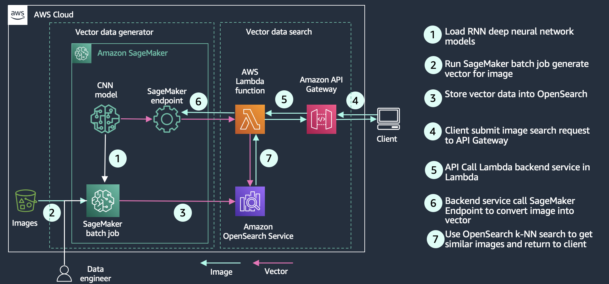
Multimodal search with Amazon Bedrock

OpenSearch Service 2.11 launches the support of multimodal search that allows you to search text and image data using multimodal embedding models. To generate vector embeddings, you need to create an ingest pipeline that contains a text_image_embedding processor, which converts the text or image binaries in a document field to vector embeddings. You can use the neural query clause, either in the k-NN plugin API or Query DSL queries, to do a combination of text and images searches. You can use the new OpenSearch Service integration features to quickly start with multimodal search.

Neural sparse retrieval

Neural sparse search, a new efficient method of semantic retrieval, is available in OpenSearch Service 2.11. Neural sparse search operates in two modes: bi-encoder and document-only. With the bi-encoder mode, both documents and search queries are passed through deep encoders. In document-only mode, only documents are passed through deep encoders, while search queries are tokenized. A document-only sparse encoder generates an index that is 10.4% of the size of a dense encoding index. For a bi-encoder, the index size is 7.2% of the size of a dense encoding index. Neural sparse search is enabled by sparse encoding models that create sparse vector embeddings: a set of <token: weight> pairs representing the text entry and its corresponding weight in the sparse vector. To learn more about the pre-trained models for sparse neural search, refer to Sparse encoding models.

Neural sparse search reduces costs, improves search relevance, and has lower latency. You can use the new OpenSearch Service integrations features to quickly start with neural sparse search.

OpenSearch Ingestion updates

OpenSearch Ingestion is a fully managed and auto scaled ingestion pipeline that delivers your data to OpenSearch Service domains and OpenSearch Serverless collections. Since its release in 2023, OpenSearch Ingestion continues to add new features to make it straightforward to transform and move your data from supported sources to downstream destinations like OpenSearch Service, OpenSearch Serverless, and Amazon S3.

New migration features in OpenSearch Ingestion

In November 2023, OpenSearch Ingestion announced the release of new features to support data migration from self-managed Elasticsearch version 7.x domains to the latest versions of OpenSearch Service.

OpenSearch Ingestion also supports the migration of data from OpenSearch Service managed domains running OpenSearch version 2.x to OpenSearch Serverless collections.

Learn how you can use OpenSearch Ingestion to migrate your data to OpenSearch Service.

Improve data durability with OpenSearch Ingestion

In November 2023, OpenSearch Ingestion introduced persistent buffering for push-based sources likes HTTP sources (HTTP, Fluentd, FluentBit) and OpenTelemetry collectors.

By default, OpenSearch Ingestion uses in-memory buffering. With persistent buffering, OpenSearch Ingestion stores your data in a disk-based store that is more resilient. If you have existing ingestion pipelines, you can enable persistent buffering for these pipelines, as shown in the following screenshot.

Support of new plugins

In early 2023, OpenSearch Ingestion added support for Amazon Managed Streaming for Apache Kafka (Amazon MSK). OpenSearch Ingestion uses the Kafka plugin to stream data from Amazon MSK to OpenSearch Service managed domains or OpenSearch Serverless collections. To learn more about setting up Amazon MSK as a data source, see Using an OpenSearch Ingestion pipeline with Amazon Managed Streaming for Apache Kafka.

OpenSearch Serverless updates

OpenSearch Serverless continued to enhance your serverless experience with OpenSearch by introducing the support of a new collection of type vector search to store embeddings and run similarity search. OpenSearch Serverless now supports shard replica scaling to handle spikes in query throughput. And if you are using a time series collection, you can now set up your custom data retention policy to match your data retention requirements.

Vector Engine for OpenSearch Serverless

In November 2023, we launched the vector engine for Amazon OpenSearch Serverless. The vector engine makes it straightforward to build modern ML-augmented search experiences and generative artificial intelligence (generative AI) applications without needing to manage the underlying vector database infrastructure. It also enables you to run hybrid search, combining vector search and full-text search in the same query, removing the need to manage and maintain separate data stores or a complex application stack.

OpenSearch Serverless lower-cost dev and test environments

OpenSearch Serverless now supports development and test workloads by allowing you to avoid running a replica. Removing replicas eliminates the need to have redundant OCUs in another Availability Zone solely for availability purposes. If you are using OpenSearch Serverless for development and testing, where availability is not a concern, you can drop your minimum OCUs from 4 to 2.

OpenSearch Serverless supports automated time-based data deletion using data lifecycle policies

In December 2023, OpenSearch Serverless announced support for managing data retention of time series collections and indexes. With the new automated time-based data deletion feature, you can specify how long you want to retain data. OpenSearch Serverless automatically manages the lifecycle of the data based on this configuration. To learn more, refer to Amazon OpenSearch Serverless now supports automated time-based data deletion.

OpenSearch Serverless announced support for scaling up replicas at shard level

At launch, OpenSearch Serverless supported increasing capacity automatically in response to growing data sizes. With the new shard replica scaling feature, OpenSearch Serverless automatically detects shards under duress due to sudden spikes in query rates and dynamically adds new shard replicas to handle the increased query throughput while maintaining fast response times. This approach proves to be more cost-efficient than simply adding new index replicas.

AWS user notifications to monitor your OCU usage

With this launch, you can configure the system to send notifications when OCU utilization is approaching or has reached maximum configured limits for search or ingestion. With the new AWS User Notification integration, you can configure the system to send notifications whenever the capacity threshold is breached. The User Notification feature eliminates the need to monitor the service constantly. For more information, see Monitoring Amazon OpenSearch Serverless using AWS User Notifications.

Enhance your experience with OpenSearch Dashboards

OpenSearch 2.9 in OpenSearch Service introduced new features to make it straightforward to quickly analyze your data in OpenSearch Dashboards. These new features include the new out-of-the box, preconfigured dashboards with OpenSearch Integrations, and the ability to create alerting and anomaly detection from an existing visualization in your dashboards.

OpenSearch Dashboard integrations

OpenSearch 2.9 added the support of OpenSearch integrations in OpenSearch Dashboards. OpenSearch integrations include preconfigured dashboards so you can quickly start analyzing your data coming from popular sources such as AWS CloudFront, AWS WAF, AWS CloudTrail, and Amazon Virtual Private Cloud (Amazon VPC) flow logs.

Alerting and anomalies in OpenSearch Dashboards

In OpenSearch Service 2.9, you can create a new alerting monitor directly from your line chart visualization in OpenSearch Dashboards. You can also associate the existing monitors or detectors previously created in OpenSearch to the dashboard visualization.

This new feature helps reduce context switching between dashboards and both the Alerting or Anomaly Detection plugins. Refer to the following dashboard to add an alerting monitor to detect drops in average data volume in your services.

OpenSearch expands geospatial aggregations support

With OpenSearch version 2.9, OpenSearch Service added the support of three types of geoshape data aggregation through API: geo_bounds, geo_hash, and geo_tile.

The geoshape field type provides the possibility to index location data in different geographic formats such as a point, a polygon, or a linestring. With the new aggregation types, you have more flexibility to aggregate documents from an index using metric and multi-bucket geospatial aggregations.

OpenSearch Service operational updates

OpenSearch Service removed the need to run blue/green deployment when changing the domain managed nodes. Additionally, the service improved the Auto-Tune events with the support of new Auto-Tune metrics to track the changes within your OpenSearch Service domain.

OpenSearch Service now lets you update domain manager nodes without blue/green deployment

As of early H2 of 2023, OpenSearch Service allowed you to modify the instance type or instance count of dedicated cluster manager nodes without the need for blue/green deployment. This enhancement allows quicker updates with minimal disruption to your domain operations, all while avoiding any data movement.

Previously, updating your dedicated cluster manager nodes on OpenSearch Service meant using a blue/green deployment to make the change. Although blue/green deployments are meant to avoid any disruption to your domains, because the deployment utilizes additional resources on the domain, it is recommended that you perform them during low-traffic periods. Now you can update cluster manager instance types or instance counts without requiring a blue/green deployment, so these updates can complete faster while avoiding any potential disruption to your domain operations. In cases where you modify both the domain manager instance type and count, OpenSearch Service will still use a blue/green deployment to make the change. You can use the dry-run option to check whether your change requires a blue/green deployment.

Enhanced Auto-Tune experience

In September 2023, OpenSearch Service added new Auto-Tune metrics and improved Auto-Tune events that give you better visibility into the domain performance optimizations made by Auto-Tune.

Auto-Tune is an adaptive resource management system that automatically updates OpenSearch Service domain resources to improve efficiency and performance. For example, Auto-Tune optimizes memory-related configuration such as queue sizes, cache sizes, and Java virtual machine (JVM) settings on your nodes.

With this launch, you can now audit the history of the changes, as well as track them in real time from the Amazon CloudWatch console.

Additionally, OpenSearch Service now publishes details of the changes to Amazon EventBridge when Auto-Tune settings are recommended or applied to an OpenSearch Service domain. These Auto-Tune events will also be visible on the Notifications page on the OpenSearch Service console.

Accelerate your migration to OpenSearch Service with the new Migration Assistant solution

In November 2023, the OpenSearch team launched a new open-source solution—Migration Assistant for Amazon OpenSearch Service. The solution supports data migration from self-managed Elasticsearch and OpenSearch domains to OpenSearch Service, supporting Elasticsearch 7.x (<=7.10), OpenSearch 1.x, and OpenSearch 2.x as migration sources. The solution facilitates the migration of the existing and live data between source and destination.

Conclusion

In this post, we covered the new releases in OpenSearch Service to help you innovate your business with search, observability, security analytics, and migrations. We provided you with information about when to use each new feature in OpenSearch Service, OpenSearch Ingestion, and OpenSearch Serverless.

Learn more about OpenSearch Dashboards and OpenSearch plugins and the new exciting OpenSearch assistant using OpenSearch playground.

Check out the features described in this post, and we appreciate you providing us your valuable feedback.

About the Authors

Jon Handler is a Senior Principal Solutions Architect at Amazon Web Services based in Palo Alto, CA. Jon works closely with OpenSearch and Amazon OpenSearch Service, providing help and guidance to a broad range of customers who have search and log analytics workloads that they want to move to the AWS Cloud. Prior to joining AWS, Jon’s career as a software developer included 4 years of coding a large-scale, ecommerce search engine. Jon holds a Bachelor of the Arts from the University of Pennsylvania, and a Master of Science and a PhD in Computer Science and Artificial Intelligence from Northwestern University.

Hajer Bouafif is an Analytics Specialist Solutions Architect at Amazon Web Services. She focuses on Amazon OpenSearch Service and helps customers design and build well-architected analytics workloads in diverse industries. Hajer enjoys spending time outdoors and discovering new cultures.

Aruna Govindaraju is an Amazon OpenSearch Specialist Solutions Architect and has worked with many commercial and open source search engines. She is passionate about search, relevancy, and user experience. Her expertise with correlating end-user signals with search engine behavior has helped many customers improve their search experience.

Prashant Agrawal is a Sr. Search Specialist Solutions Architect with Amazon OpenSearch Service. He works closely with customers to help them migrate their workloads to the cloud and helps existing customers fine-tune their clusters to achieve better performance and save on cost. Before joining AWS, he helped various customers use OpenSearch and Elasticsearch for their search and log analytics use cases. When not working, you can find him traveling and exploring new places. In short, he likes doing Eat → Travel → Repeat.

Muslim Abu Taha is a Sr. OpenSearch Specialist Solutions Architect dedicated to guiding clients through seamless search workload migrations, fine-tuning clusters for peak performance, and ensuring cost-effectiveness. With a background as a Technical Account Manager (TAM), Muslim brings a wealth of experience in assisting enterprise customers with cloud adoption and optimize their different set of workloads. Muslim enjoys spending time with his family, traveling and exploring new places.