Tag Archives: Cloud Cost Optimization

Save up to 24% on Amazon Redshift Serverless compute costs with Reservations

Post Syndicated from Satesh Sonti original https://aws.amazon.com/blogs/big-data/save-up-to-24-on-amazon-redshift-serverless-compute-costs-with-reservations/

 Amazon Redshift Serverless makes it convenient to run and scale analytics without managing clusters, offering a flexible pay-as-you-go model. With Redshift Serverless Reservations, you can optimize compute costs and improve cost predictability for your Redshift Serverless workloads.

In this post, you learn how Amazon Redshift Serverless Reservations can help you lower your data warehouse costs. We explore ways to determine the optimal number of RPUs to reserve, review example scenarios, and discuss important considerations when purchasing these reservations.

How Amazon Redshift Serverless Reservations work

Amazon Redshift measures data warehouse capacity in Redshift Processing Units (RPUs). You pay for the workloads you run in RPU-hours on a per-second basis (with a 60-second minimum charge). 1 RPU provides 16 GB of memory. You can commit to a specific number of Redshift Processing Units (RPUs) for a one-year term. Two payment options are available: a no-upfront option with a 20% discount off on-demand rates, or an all-upfront option with a 24% discount. The reserved amount of RPUs is billed 24 hours a day, seven days a week

Amazon Redshift Serverless Reservations are managed at the AWS payer account level and can be shared across multiple AWS accounts. Any usage beyond your committed RPU level is charged at standard on-demand rates. You can purchase Serverless Reservations through either the Amazon Redshift console or the Amazon Redshift Serverless Reservations API using the create-reservation command.

Key benefits of Amazon Redshift Serverless Reservations

The following are some of the key benefits of subscribing to Redshift Serverless Reservations.

  • Cost savings through commitment: Redshift Serverless Reservations help you reduce your overall Redshift Serverless spend compared to on-demand (non-reserved) usage.
  • Centralized management: Supports reservation administration at the AWS payer account level for simplified governance and visibility across your organization.
  • Per-second metering with hourly billing: Offers per-second metering with hourly billing, so that you only pay for what you use. This cost-effective pricing model eliminates wasted resources and unnecessary charges, lowering your Amazon Redshift Serverless spend.
  • Predictable costs: The 24 hours a day, 7 days a week billing model offers stable monthly costs that simplify forecasting and budgeting.
  • Sharing capabilities between multiple AWS accounts: Enhances collaboration across different teams and departments, enabling improved resource utilization throughout your organization.

Determining optimal RPU reservation

You can determine your RPU reservation level through your serverless usage history and the AWS Billing and Cost Management recommendations.

Serverless usage history

You can use the Redshift Serverless Dashboard, which provides a detailed view of your workgroup and namespace activities. The dashboard helps you to analyze trends and patterns in your data warehouse usage. You can easily monitor your RPU capacity usage and total compute usage, helping you make informed decisions about resource allocation. For more granular analysis, you have the option to query the SYS_SERVERLESS_USAGE system table, which provides detailed historical usage data. To optimize costs while ensuring performance, you can reserve the minimum consistent RPUs used per hour by analyzing the usage patterns across all your workgroups.

AWS Billing and Cost Management recommendations

You can use AWS Billing and Cost Management to help you estimate your capacity needs:

  1. Navigate to your Billing and Cost Management dashboard.
  2. On the left navigation pane, expand Reservations.
  3. Choose Recommendations.
  4. Select Redshift in the Service drop down menu.
  5. Choose required Term, Payment option, and Based on the past to select the history to determine reservation recommendations.
  6. You will find the recommendations in the Recommendations section. The following is an example screen:

Recommendations Section

The following example shows a Redshift Serverless purchase recommendation from AWS Cost Management. The interface displays a specific recommendation to buy Reserved Instances with key details including the term length, AWS Region, payment option, and expected utilization rate. The recommendation includes upfront and recurring cost information, with a direct link to the Amazon Redshift console for implementation.

RS Serverless RPU instances

If reservations are not recommended based on your usage, then you will see “Based on your selections, no purchase recommendations are available for you at this time. Adjust your selections to view recommendation” message under the Recommended actions section.

Cost Explorer generates your reservation recommendations by identifying your On-demand usage during a specific period and identifying the best number of reservations to purchase to maximize your estimated savings.

Disclaimer: The approaches described above provide an estimate of your optimal RPU reservation level. Actual results may vary depending on workload patterns, peak usage, and utilization variability. Your RPU commitment may not always yield the maximum available discount percentage, as savings depend on how closely your Redshift Serverless Reserved RPUs aligns with real usage over time. This recommendation does not guarantee the cost for your actual use of AWS services.

For more details visit Accessing reservation recommendations.

Real-world scenarios

Let’s examine two different scenarios to understand how reservations can help you optimize costs, we’ll walk through the scenario of a single Redshift Serverless workgroup and a scenario with multiple Redshift serverless workgroups.

Scenario 1: Single Redshift Serverless workgroup

Let’s consider you have only one Redshift Serverless workgroup in your environment and the workload is spread as described in the following table.

In the table, hourly RPU consumption metrics for workgroup1 across different time intervals. The data shows a reservation of 64 RPUs with no upfront payment option, which provides a 20% discount. The table breaks down the compute usage into two categories: Reserved compute, consistently showing 64 RPUs across all hours, and On-demand compute, which varies based on actual consumption above the reserved capacity. The bottom row displays the Total charged RPUs, which reflects the final billing after applying the reserved instance discount. This helps visualize how the workload utilizes the reserved capacity and any additional on-demand usage throughout the specified time period.The total actual RPU consumption is 1,664 and the total charged consumption is 1,484.8. This configuration results in a 10.7% net discount.

Scenario 2: Multiple Redshift Serverless workgroups

In this scenario, you have multiple Redshift serverless workgroup in your environment and the workload is spread as described in the following table.

Similar to the previous single workgroup scenario, you can see hourly RPU consumption metrics for workgroups across different time intervals. In this scenario, you have also opted for 64 RPUs reserved with no upfront option, which applies a 20% discount to the workload. However, you can notice that the total consumption across workgroups matches the total reserved RPUs. This maximizes your total savings even though individual workgroups consumed less than the total RPUs reserved at the payer account level.

The total actual RPU consumption is 1,536 (768+512+256) across workgroups and the total charged consumption is 1,228.8. This configuration results in a 20% net discount.

You can use the following query to find the average RPUs consumed in each hour in a workgroup.

SELECT
date_trunc('hour',end_time) AS run_hr,
avg(compute_capacity)
FROM SYS_SERVERLESS_USAGE
GROUP BY 1
ORDER BY 1

You can use the output of this query to populate a spreadsheet with a similar structure as the ones used in the previous scenarios.

Considerations

We recommend you consider the following when using Redshift Serverless Reservations:

  • Start conservatively: Avoid over-purchasing Serverless Reservations RPUs. It’s best to begin with a minimum base RPU level or align your commitment to the average RPU usage across all Redshift Serverless workgroups under your AWS payer and linked accounts.
  • Reservations are immutable: Once purchased, Redshift Serverless Reservations can’t be changed or deleted. However, you can add additional reservations later to increase your coverage as your workloads grow.
  • Discount sharing control: The management account in an AWS Organization can disable Reserved Instance or Savings Plan discount sharing for any linked accounts, including itself. See the AWS documentation for details.
  • Automatic discount application: Redshift Serverless Reservations billing model automatically applies all the reserved RPU discount to your workloads before using on-demand cost, helping you save on costs.
  • Reservations are Regional: They apply only within the AWS Region where they are purchased and cannot be shared across Regions.
  • Handling excess usage: If your workload exceeds the number of reserved RPUs, the additional usage is billed at the standard on-demand rate.
  • Use a 30 to 60-day window for recommendations: To receive the most accurate reservation recommendations, we suggest using a 30- to 60-day usage window in the Billing and Cost Management console, under Reservations, in the Recommendations section. This approach assumes that your typical production workloads have been running during that period so that the recommendations reflect real-world usage.

Conclusion

In this post, we described how Amazon Redshift Serverless Reservations provide a way to reduce your data warehouse costs while maintaining the flexibility of Redshift serverless pricing. By carefully planning your Amazon Redshift Serverless Reservation strategy and monitoring usage patterns, you can achieve up to 24% cost savings for your Redshift Serverless analytics workloads. For detailed documentation, see Billing for serverless reservations.


About the authors

Satesh Sonti

Satesh Sonti

Satesh is a Principal Specialist Solutions Architect based out of Atlanta, specializing in building enterprise data platforms, data warehousing, and analytics solutions. He has over 20 years of experience in building data assets and leading complex data platform programs for banking and insurance clients across the globe.

Ashish Agrawal

Ashish Agrawal

Ashish is a Principal Product Manager with Amazon Redshift, building cloud-based data warehouses and analytics cloud services. Ashish has over 25 years of experience in IT. Ashish has expertise in data warehouses, data lakes, and platform as a service. Ashish has been a speaker at worldwide technical conferences.

Decrease your storage costs with Amazon OpenSearch Service index rollups

Post Syndicated from Luis Tiani original https://aws.amazon.com/blogs/big-data/decrease-your-storage-costs-with-amazon-opensearch-service-index-rollups/

Amazon OpenSearch Service is a fully managed service to support search, log analytics, and generative AI Retrieval Augment Generation (RAG) workloads in the AWS Cloud. It simplifies the deployment, security, and scaling of OpenSearch clusters. As organizations scale their log analytics workloads by continuously collecting and analyzing vast amounts of data, they often struggle to maintain quick access to historical information while managing costs effectively. OpenSearch Service addresses these challenges through its tiered storage options: hot, UltraWarm, and cold storage. These storage tiers are great options to help optimize costs and offer a balance between performance and affordability, so organizations can manage their data more efficiently. Organizations can choose between these different storage tiers by keeping data in expensive hot storage for quick access or moving it to cheaper cold storage with limited accessibility. This trade-off becomes particularly challenging when organizations need to analyze both recent and historical data for compliance, trend analysis, or business intelligence.

In this post, we explore how to use index rollups in Amazon OpenSearch Service to address this challenge. This feature helps organizations efficiently manage their historical data by automatically summarizing and compressing older data while maintaining its analytical value, significantly reducing storage costs in any storage tier without sacrificing the ability to query historical information effectively.

Index rollups overview

Index rollups provide a mechanism to aggregate historical data into summarized indexes at specified time intervals. This feature is particularly useful for time series data where the granularity of older data can be reduced while maintaining meaningful analytics capabilities.

Key benefits include:

  • Reduced storage costs (varies by granularity level), for example:
    • Larger savings when aggregating from seconds to hours
    • Moderate savings when aggregating from seconds to minutes
  • Improved query performance of historical data
  • Maintained data accessibility for long-term analytics
  • Automated data summarization process

Index rollups are part of a comprehensive data management strategy. The real cost savings come from properly managing your data lifecycle in conjunction with rollups. To achieve meaningful cost reductions, you must remove or move the original data to a lower-cost storage tier after creating the rollup.

For customers already using Index State Management (ISM) to move older data to UltraWarm or cold tiers, rollups can provide significant additional benefits. By aggregating data at higher time intervals before moving it to lower-cost tiers, you can dramatically reduce the volume of data in these tiers, leading to further cost savings. This strategy is particularly effective for workloads with large amounts of time series data, typically measuring in terabytes or petabytes. The larger your data volume, the more impactful your savings will be when implementing rollups correctly.

Index rollups can be implemented using ISM policies through the OpenSearch Dashboards UI or the OpenSearch API. Index rollups require OpenSearch or Elasticsearch 7.9 or later.

The decision to use different storage tiers requires careful consideration of an organization’s specific needs, balancing the desire for cost savings with the requirement for data accessibility and performance. As data volumes continue to grow and analytics become increasingly important, finding the right storage strategy becomes crucial for businesses to remain competitive and compliant while managing their budgets effectively.

In this post, we consider a scenario with a large volume of time series data that can be aggregated using the Rollup API. With rollups, you have the flexibility to either store aggregated data in the hot tier for rapid access or aggregate and promote it to more cost-effective tiers such as UltraWarm or cold storage. This approach allows for efficient data and index lifecycle management while optimizing both performance and cost.

Index rollups are often confused with index rollovers, which are automated OpenSearch Service operations that create new indexes when specified thresholds are met, for example by age, size, or document count. This feature maintains raw data while optimizing cluster performance through controlled index growth. For example, rolling over when an index reaches 50 GB or is 30 days old.

Use cases for index rollups

Index rollups are ideal for scenarios where you need to balance storage costs with data granularity, such as:

  • Time series data that requires different granularity levels over time – For example, Internet of Things (IoT) sensor data where real-time precision matters only for the most recent data.
    • Traditional approach – It is common for users to keep all data in expensive hot storage for instant accessibility. However, this isn’t optimal for cost.
    • Recommended – Retain recent (per second) data in hot storage for immediate access. For older periods, store aggregated (hourly or daily) data using index rollups. Move or delete the higher-granularity old data from the hot tier. This balances accessibility and cost-effectiveness.
  • Historical data with cost-optimization needs – For example, system performance metrics where overall trends are more valuable than precise values over time.
    • Traditional approach – It is common for users to store all performance metrics at full granularity indefinitely, consuming excessive storage space. We don’t recommend storing data indefinitely. Implement a data retention policy based on your specific business needs and compliance requirements.
    • Recommended – Maintain detailed metrics for recent monitoring (last 30 days) and aggregate older data into hourly or daily summaries. This preserves the trend analysis capability while significantly reducing storage costs.
  • Log data with infrequent historical access and low value – For example, application error logs where detailed investigation is primarily needed for recent incidents.
    • Traditional approach – It is common for users to keep all log entries at full detail, regardless of age or access frequency.
    • Recommended – Preserve detailed logs for an active troubleshooting period (for example, 1 week) and maintain summarized error patterns and statistics for older periods. This enables historical pattern analysis while reducing storage overhead.

Schema design

A well-planned schema is crucial for successful rollup implementation. Proper schema design makes sure your rolled-up data remains valuable for analysis while maximizing storage savings. Consider the following key aspects:

  • Identify fields required for long-term analysis – Carefully select fields that provide meaningful insights over time, avoiding unnecessary data retention.
  • Define aggregation types for each field, such as min, max, sum, and average – Choose appropriate aggregation methods that preserve the analytical value of your data.
  • Determine which fields can be excluded from rollups – Reduce storage costs by omitting fields that don’t contribute to long-term analysis.
  • Consider mapping compatibility between source and target indexes – Provide successful data transition without mapping conflicts. This involves:
    • Matching data types (for example, date fields remain as date in rollups)
    • Handling nested fields appropriately
    • Ensuring all required fields are included in the rollup
    • Considering the impact of analyzed vs. non-analyzed fields
    • Incompatible mappings can lead to failed rollup jobs or incorrect data aggregation.

Functional and non-functional requirements

Before implementing index rollups, consider the following:

  • Data access patterns – When implementing data rollup strategies, it’s crucial to first analyze data access patterns, including query frequency and usage periods, to determine optimal rollup intervals. This analysis should lead to specific granularity metrics, such as deciding between hourly or daily aggregations, while establishing clear thresholds based on both data volume and query requirements. These decisions should be documented alongside specific aggregation rules for each data type.
  • Data growth rate – Storage optimization begins with calculating your current dataset size and its growth rate. This information helps quantify potential space reductions across different rollup strategies. Performance metrics, particularly expected query response times, should be defined upfront. Additionally, establish monitoring KPIs focusing on latency, throughput, and resource usage to make sure the system meets performance expectations.
  • Compliance or data retention requirements – Retention planning requires careful consideration of regulatory requirements and business needs. Develop a clear retention policy that specifies how long to keep different types of data at various granularity levels. Implement systematic processes for archiving or deleting older data and maintain detailed documentation of storage costs across different retention periods.
  • Resource utilization and planning – For successful implementation, proper cluster capacity planning is essential. This involves accurately sizing computing resources, including CPU, RAM, and storage requirements. Define specific time windows for executing rollup jobs to minimize impact on regular operations. Set clear resource utilization thresholds and implement proactive capacity monitoring. Finally, develop a scalability plan that accounts for both horizontal and vertical growth to accommodate future needs.

Operational requirements

Proper operational planning facilitates smooth ongoing management of your rollup implementation. This is essential for maintaining data reliability and system health:

  • Monitoring – You must monitor rollup jobs for their accuracy and desired results. This means implementing automated checks that validate data completeness, aggregation accuracy, and job execution status. Set up alerts for failed jobs, data inconsistencies, or when aggregation results fall outside expected ranges.
  • Scheduling hours – Schedule rollup operations during periods of low system usage, typically during off-peak hours. Document these maintenance windows clearly and communicate them to all stakeholders. Include buffer time for potential issues and establish clear procedures for what happens if a maintenance window needs to be extended.
  • Backup and recovery – OpenSearch Service takes automated snapshots of your data at 1-hour intervals. But you can define and implement comprehensive backup procedures using snapshot management functionality to support your Recovery Time Objective (RTO) and Recovery Point Objective (RPO).

Your RPO can be customized through different rollup schedules based on index patterns. This flexibility helps you define varied data loss tolerance levels according to your data’s criticality. For mission-critical indexes, you can configure more frequent rollups, while maintaining less frequent schedules for analytical data.

You can tailor RTO management in OpenSearch per index pattern through backup and replication options. For critical rollup indexes, implementing cross-cluster replication maintains up-to-date copies, significantly reducing recovery time. Other indexes might use standard backup procedures, balancing recovery speed with operational costs. This flexible approach helps you optimize both storage costs and recovery objectives based on your specific business requirements for different types of data within your OpenSearch deployment.

Before implementing rollups, audit all applications and dashboards that use the data being aggregated. Update queries and visualizations to accommodate the new data structure. Test these changes thoroughly in a staging environment to confirm they continue to provide accurate results with the rolled-up data. Create a rollback plan in case of unexpected issues with dependent applications.

In the following sections, we walk through the steps to create, run, and monitor a rollup job.

Create a rollup job

As discussed in previous sections, there are some considerations when choosing good candidates for index rollup usage. Building on this concept, identify your indexes to roll up their data and create the jobs.The following code is an example of creating a basic rollup job:

PUT /_plugins/_rollup/jobs/sensor_hourly_rollup
{
  "rollup": {
    "rollup_id": "sensor_1_hour_rollup",
    "enabled": true,
    "schedule": {
      "interval": {
        "start_time": 1746632400,        
        "period": 1,
        "unit": "hours",
        "schedule_delay": 0
      }
    },
    "description": "Rolls up sensor data 1 hourly per device_id",
    "source_index": "sensor-*",           
    "target_index": "sensor_rolled_hour",
    "page_size": 1000,
    "delay": 0,
    "continuous": true,
    "dimensions": [
      {
        "date_histogram": {
          "fixed_interval": "1h",
          "source_field": "timestamp",
          "target_field": "timestamp",
          "timezone": "UTC"
        }
      },
      {
        "terms": {
          "source_field": "device_id",
          "target_field": "device_id"
        }
      }
    ],
    "metrics": [
      {
        "source_field": "temperature",
        "metrics": [
          { "avg": {} },
          { "min": {} },
          { "max": {} }
        ]
      },
      {
        "source_field": "humidity",
        "metrics": [
          { "avg": {} },
          { "min": {} },
          { "max": {} }
        ]
      },
      {
        "source_field": "pressure",
        "metrics": [
          { "avg": {} },
          { "min": {} },
          { "max": {} }
        ]
      },
      {
        "source_field": "battery",
        "metrics": [
          { "avg": {} },
          { "min": {} },
          { "max": {} }
        ]
      }
    ]
  }
}

This rollup job processes IoT sensor data, aggregating readings from the sensor-* index pattern into hourly summaries stored in sensor_rolled_hour. It maintains device-level granularity while calculating average, minimum, and maximum values for temperature, humidity, pressure, and battery levels. The job executes hourly, processing 1,000 documents per batch.

The preceding code assumes that the device_id field is of type keyword; note that aggregation can’t be performed on the text field.

Start the rollup job

After you create the job, it will automatically be scheduled based on the job’s configuration (refer to the schedule: part of the job example code in the previous section). However, you can also trigger the job manually using the following API call:

POST _plugins/_rollup/jobs/sensor_hourly_rollup/_start

The following is an example of the results:

{
  "acknowledged": true
}

Monitor progress

Using Dev Tools, run the following command to monitor the progress:

GET _plugins/_rollup/jobs/sensor_hourly_rollup/_explain

The following is an example of the results:

{
  "sensor_hourly_rollup": {
    "metadata_id": "pCDjMZcBgTxYF90dWEfP",
    "rollup_metadata": {
      "rollup_id": "sensor_hourly_rollup",
      "last_updated_time": 1749043472416,
      "continuous": {
        "next_window_start_time": 1749043440000,
        "next_window_end_time": 1749043560000
      },
      "status": "started",
      "failure_reason": null,
      "stats": {
        "pages_processed": 374603,
        "documents_processed": 390,
        "rollups_indexed": 200,
        "index_time_in_millis": 789,
        "search_time_in_millis": 402202
      }
    }
  }
}  

The GET _plugins/_rollup/jobs/sensor_hourly_rollup/_explain command shows the current status and statistics of the sensor_hourly_rollup job. The response shows important statistics such as the number of processed documents, indexed rollups, time spent on indexing and searching, and records of any failures. The status indicates whether the job is active (started) or stopped (stopped) and shows the last processed timestamp. This information is crucial for monitoring the efficiency and health of the rollup process, helping administrators track progress, identify potential issues or bottlenecks, and confirm the job is operating as expected. Regular checks of these statistics can help in optimizing the rollup job’s performance and maintaining data integrity.

Real-world example

Let’s consider a scenario where a company collects IoT sensor data, ingesting 240 GB of data per day to an OpenSearch cluster, which totals 7.2 TB per month.

The following is an example record:

"_source": {
          "timestamp": "2024-01-01T10:00:00Z",
          "device_id": "sensor_001",
          "temperature": 26.1,
          "humidity": 43,
          "pressure": 1009.3,
          "battery": 90
}

Assume you have a time series index with the following configuration:

  • Ingest rate: 10 million documents per hour
  • Retention period: 30 days
  • Each document size: Approximately 1 KB

The total storage without rollups is as follows:

  • Per-day storage size: 10,000,000 docs per hour × ~1 KB × 24 hours per day = ~240 GB
  • Per-month storage size: 240 GB × 30 days = ~7.2 TB

The decision to implement rollups should be based on a cost-benefit analysis. Consider the following:

  • Current storage costs vs. potential savings
  • Compute costs for running rollup jobs
  • Value of granular data over time
  • Frequency of historical data access

For smaller datasets (for example, less than 50 GB/day), the benefits might be less significant. As data volumes grow, the cost savings become more compelling.

Rollup configuration

Let’s roll up the data with the following configuration:

  • From 1-minute granularity to 1-hour granularity
  • Aggregating average, min, and max, grouped by device_id
  • Reducing 60 documents per minute to 1 rollup document per minute

The new document count per hour is as follows:

  • Per-hour documents: 10,000,000/60 = 166,667 docs per hour
  • Assuming each rollup document is 2 KB (extra metadata), total rollup storage: 166,667 docs per hour × 24 hours per day × 30 days × 2KB ˜= 240 GB/month

Verify all required data exists in the new rolled index, then delete the original index to remove raw data manually or by using ISM policies (as discussed in the next section).

Execute the rollup job following the preceding instructions to aggregate data into the new rolled up index. To view your aggregated results, run the following code:

GET sensor_rolled_hour/_search
{
  "size": 0,
  "aggs": {
    "per_device": {
      "terms": {
        "field": "device_id",
        "size": 200,
        "shard_size": 200
      },
      "aggs": {
        "temperature_avg": {
          "avg": {
            "field": "temperature"
          }
        },
        "temperature_min": {
          "min": {
            "field": "temperature"
          }
        },
        "temperature_max": {
          "max": {
            "field": "temperature"
          }
        }
      }
      }
    }
  } 

The following code shows the example results:

"aggregations": {
    "per_device": {
      "doc_count_error_upper_bound": 0,
      "sum_other_doc_count": 0,
      "buckets": [
        {
          "key": "sensor_001",
          "doc_count": 98,
          "temperature_min": {
            "value": 24.100000381469727
          },
          "temperature_avg": {
            "value": 26.287754603794642
          },
          "temperature_max": {
            "value": 27.5
          }
        },
        {
          "key": "sensor_002",
          "doc_count": 98,
          "temperature_min": {
            "value": 20.600000381469727
          },
          "temperature_avg": {
            "value": 22.192856146364797
          },
          "temperature_max": {
            "value": 22.799999237060547
          }
        },...]

This document represents the rolled-up data for sensor_001 and sensor_002 during a 1-hour period. It aggregates 1 hour of sensor readings into a single record, storing minimum, average, and maximum values for temperature levels. The record includes metadata about the rollup process and timestamps for data tracking. This aggregated format significantly reduces storage requirements while maintaining essential statistical information about the sensor’s performance during that hour.

We can calculate the storage savings as follows:

  • Original storage: 7.2 TB (or 7200 GB)
  • Post-rollup storage: 240 GB
  • Storage savings: ((7.2 TB – 240 GB)/7.2 GB) × 100 = 96.67% savings

Using OpenSearch rollups as demonstrated in this example, you can achieve approximately 96% storage savings while preserving important aggregate insights.

The aggregation levels and document sizes can be customized according to your specific use case requirements.

Automate rollups with ISM

To fully realize the benefits of index rollups, automate the process using ISM policies. The following code is an example that implements a rollup strategy based on the given scenario:

PUT _plugins/_ism/policies/sensor_rollup_policy
{
  "policy": {
    "description": "Roll up sensor data and delete original",
    "default_state": "hot",
    "ism_template": {
      "index_patterns": ["sensor-*"],
      "priority": 100
    },
    "states": [
      {
        "name": "hot",
        "actions": [],
        "transitions": [
          {
            "state_name": "rollup",
            "conditions": {
              "min_index_age": "1d"
            }
          }
        ]
      },
      {
        "name": "rollup",
        "actions": [
          {
            "rollup": {
              "ism_rollup": {
                "target_index": "sensor_rolled_minutely",
                "description": "Rollup sensor data to minutely aggregations",
                "page_size": 1000,
                "dimensions": [
                  {
                    "date_histogram": {
                      "fixed_interval": "1m",
                      "source_field": "timestamp",
                      "target_field": "timestamp"
                    }
                  },
                  {
                    "terms": {
                      "source_field": "device_id",
                      "target_field": "device_id"
                    }
                  }
                ],
                "metrics": [
                  {
                    "source_field": "temperature",
                    "metrics": [{ "avg": {} }, { "min": {} }, { "max": {} }]
                  },
                  {
                    "source_field": "humidity",
                    "metrics": [{ "avg": {} }, { "min": {} }, { "max": {} }]
                  }
                ]
              }
            }
          }
        ],
        "transitions": [
          {
            "state_name": "delete",
            "conditions": {
              "min_index_age": "2d"
            }
          }
        ]
      },
      {
        "name": "delete",
        "actions": [
          {
            "delete": {}
          }
        ]
      }
    ]
  }
}

This ISM policy automates the rollup process and data lifecycle:

    1. Applies to all indexes matching the sensor-* pattern.
    2. Keeps original data in the hot state for 1 day.
    3. After 1 day, rolls up the data into minutely aggregations. Aggregates by device_id and calculates average, minimum, and maximum for temperature and humidity.
    4. Stores rolled-up data in the sensor_rolled_minutely index.
    5. Deletes the original index 2 days after rollup.

This strategy offers the following benefits:

  • Recent data is available at full granularity
  • Historical data is efficiently summarized
  • Storage is optimized by removing original data after rollup

You can monitor the policy’s execution using the following command:

GET _plugins/_ism/policies/sensor_rollup_policy

Remember to adjust the timeframes, metrics, and aggregation intervals based on your specific requirements and data patterns.

Conclusion

Index rollups in OpenSearch Service provide a powerful way to manage storage costs while maintaining valuable historical data access. By implementing a well-planned rollup strategy, organizations can achieve significant cost savings while making sure their data remains available for analysis.

To get started, take the following next steps:

  • Review your current index patterns and data retention requirements
  • Analyze your historical data volumes and access patterns
  • Start with a proof-of-concept rollup implementation in a test environment
  • Monitor performance and storage metrics to optimize your rollup strategy
  • Move the infrequently accessed data between storage tiers:
    • Delete data you’ll no longer use
    • Automate the process using ISM policies

To learn more, refer to the following resources:


About the authors

Luis Tiani

Luis Tiani

Luis is a Sr Solutions Architect at AWS. He specializes in data and analytics topics, with extensive focus on Amazon OpenSearch Service for search, log analytics, and vector environments. Tiani has helped numerous customers across financial services, DNB, SMB, and enterprise segments in their OpenSearch adoption journey, reviewing use cases and providing architecture design and cluster sizing guidance. As a Solutions Architect, he has worked with FSI customers in developing and implementing big data and data lake solutions, app modernization, cloud migrations, and AI/ML initiatives.

Muhammad Ali

Muhammad Ali

Muhammad is a Principal Analytics (APJ Tech Lead) at AWS with over 20 years of experience in the industry. He specializes in information retrieval, data analytics, and artificial intelligence, advocating an AI-first approach while helping organizations build data-driven mindsets through technology modernization and process transformation.

Srikanth Daggumalli

Srikanth Daggumalli

Srikanth is a Senior Analytics & AI Specialist Solutions Architect in AWS. He has over a decade of experience in architecting cost-effective, performant, and secure enterprise applications that improve customer reachability and experience, using big data, AI/ML, cloud, and security technologies. He has built high-performing data platforms for major financial institutions, enabling improved customer reach and exceptional experiences. He has also built many real-time streaming log analytics, SIEM, observability, and monitoring solutions to many AWS customers, including major financial institutions, enterprise, ISV, DNB, and more.

Simplify multi-tenant encryption with a cost-conscious AWS KMS key strategy

Post Syndicated from Itay Meller original https://aws.amazon.com/blogs/architecture/simplify-multi-tenant-encryption-with-a-cost-conscious-aws-kms-key-strategy/

Organizations face diverse challenges when it comes to managing encryption keys. While some scenarios demand strict separation, there are compelling use cases where a centralized approach can streamline operations and reduce complexity. In this post, our focus is on a software-as-a-service (SaaS) provider scenario, but the principles we discuss can be adopted by large organization facing similar key management challenges.

Managing encryption across a multi-tenant, multi-service architecture presents a significant challenge. Many organizations find themselves struggling with the complexity and costs associated with provisioning separate AWS Key Management Service (AWS KMS) customer managed keys for each tenant and service. This approach, while secure, often leads to growing operational overhead and increased AWS KMS usage costs over time.

But what if there was a more efficient way?

In this post, we unveil a strategy that uses a single customer managed key (symmetric) per tenant across services. By the end of this post, you’ll learn:

  • How to implement a scalable, secure, and cost-effective encryption model
  • Techniques for using one customer managed key per tenant across multiple services and environments
  • Methods for encrypting tenant data in Amazon DynamoDB and other storage types while maintaining tenant isolation

Multi-tenant encryption requirements for SaaS providers

Data isolation is fundamental to multi-tenant SaaS architectures, serving both compliance requirements and customer confidence. Many SaaS providers need to encrypt sensitive information—from API keys and credentials to personal data—across storage solutions such as DynamoDB and Amazon Simple Storage Service (Amazon S3).

While these storage services provide default encryption at rest, they typically use a single shared key across data items. Consider DynamoDB in a shared pool model, where one table contains data from multiple tenants. In this setup, the tenant data is encrypted using the same AWS KMS Key, regardless of ownership.

KMS key represents a container for top-level key material and is uniquely defined within the KMS, for more information on the different keys involved when encrypting or decrypting data using KMS, see AWS KMS key hierarchy.

This shared-key approach often proves insufficient for SaaS providers operating under strict security and compliance frameworks. Some customers require:

  • Bring your own key (BYOK) capabilities
  • Logical isolation of their data through dedicated encryption keys

To meet these requirements, providers can implement customer-specific AWS KMS managed keys, helping to ensure that each customer’s sensitive data remains isolated and inaccessible to other tenants.

Alternatively, providers might consider a silo model with separate tables for each customer. However, this approach introduces its own challenges—as the tenant base grows, managing numerous individual tables becomes increasingly complex and service quota limits might become a constraint.

Managing growth: KMS key management at scale

When scaling a SaaS platform, empowering teams to develop services independently is crucial. A quick way to scale is to have each team develop independently using a dedicated account. This often leads to a decentralized approach where each service manages its own KMS keys per customer. However, this autonomy comes with hidden costs as your customer base and service portfolio expand.

The challenge of key proliferation

As the company grows, the number of keys multiplies with each new customer and service addition. This proliferation creates several organizational challenges:

  • Cost impact: A single AWS KMS key costs $1 monthly, increasing to a maximum of $3 per month with two or more key rotations.
  • Operational complexity: Managing many KMS keys across environments and accounts is error-prone and hard to scale.
  • Organizational waste: Duplicate efforts across teams because each develops and maintains their own code for managing customer key lifecycles.
  • Governance overhead: It becomes difficult to enforce consistent policies or track KMS key usage across multiple AWS accounts.

A streamlined approach

The solution lies in implementing a centralized key management strategy. One KMS key per tenant, maintained in a central AWS account. This approach effectively addresses the cost, operational, and governance challenges while maintaining security.

In the following sections, we explore how to implement this centralized approach and securely share KMS keys across various services and AWS accounts.

Solution overview: Centralizing tenant key management

At the heart of our solution lies a centralized tenant key management service (shown as Service A in the following figure). This service handles every aspect of customer KMS key lifecycle—from creation during tenant onboarding to managing aliases, access policies and deletion.

The service achieves secure, scalable key usage across the organization through cross-account AWS Identity and Access Management (IAM) access. It grants other services (for example, the customer-facing service in Account B in the following figure) a permission to perform specific encryption operations using tenant-specific KMS keys through role delegation. This implementation follows AWS best practices for cross-account access, utilizing IAM and AWS Security Token Service (AWS STS) role assumption as described in the AWS documentation and this blog post.

Architecture diagram showing centralizing tenant key management flow with JWT authentication, role assumption ,data encryption and saving in DynamoDB

Centralized key management in practice: Encrypting customer data

Let’s examine how this works in practice with a common scenario:

  • Service A: Our centralized tenant key management service in Account A
  • Service B: A customer-facing workload running in Account B

When a customer interacts with Service B, it needs to store sensitive information securely, whether that’s secrets, API keys, or license information in a DynamoDB table. Instead of relying on shared KMS keys or default encryption, Service B encrypts data using the customer’s dedicated KMS key managed by Service A. The process works through AWS Identity and Access Management (IAM) role delegation. Service B temporarily assumes a role (ServiceARole) in Account A, receiving fine-grained, scoped down permissions for the specific tenant’s KMS key. With these temporary credentials, Service B can perform client-side encryption operations on sensitive information using the AWS SDK or the AWS Encryption SDK.

In this blog post, we used Boto3. For more advanced use-cases requiring data key caching or keyrings, use the AWS Encryption SDK.

Solution walkthrough

Let’s expand the technical aspects of the solution depicted above. Assumptions and definitions:

  • Incoming requests include an authentication header with a JSON Web Token (JWT) that includes data identifying the current tenant’s ID. These tokens are signed by an identity provider, making sure that the JWT cannot be modified, and the tenant identity can be trusted.
  • Account A: Centralized key management service.
  • Account B: Business service that serves customer requests.
  • alias/customer-<tenant-id> is the format of the aliases in account A. Each alias points to the KMS key of the corresponding customer identified by value of <tenant-id>. Service A creates these aliases during tenant onboarding and deletes them during tenant offboarding.
  • ServiceARole: A role in Account A that can encrypt and decrypt a KMS key that has an alias prefixed with alias/customer-*. The permissions are scoped down further using session policies when ServiceBRole assumes ServiceARole.
  • ServiceBRole: A role in Account B that can assume ServiceARole in Account A to gain access to the customer’s KMS key. This will be the AWS Lambda function’s execution role.

Note that Service B’s compute layer in this case is a Lambda function, but the solution works for other compute architectures. Let’s go over the flow in more detail:

Use service with JWT

A customer who belongs to a tenant signs in to the SaaS solution and is given a JWT that identifies its tenants with a tenant ID (<tenant-id>). The customer makes an action in ServiceB and sends sensitive information.

ServiceB handles the request (in a Lambda function), verifies the JWT token and wants to:

    1. Encrypt the customer’s sensitive data
    2. Save the encrypted data along with other data in the DynamoDB table

Assume role

In this example, the Lambda function uses its execution role credentials to assume the ServiceA role in the ServiceA account. Another way to grant cross-account access to KMS keys is by using KMS grants, to learn more, see Allowing users in other accounts to use a KMS key.

Let’s review the ServiceRoleA IAM policy:

Grants encrypt and decrypt access to a KMS key using the alias/customer-* pattern.

{
  "Version": "2012-10-17",
  "Statement": [
    {
      "Sid": "AllowKMSByAlias",
      "Effect": "Allow",
      "Action": [
        "kms:Encrypt",
        "kms:Decrypt",
        "kms:GenerateDataKey*"
      ],
      "Resource": "*",
      "Condition": {
        "StringLike": {
          "kms:RequestAlias": "alias/customer-*"
        }
      }
    }
  ]
}

To encrypt tenant secrets securely and at scale, we grant application roles cross-account access to KMS keys—but only through their alias, which maps to a tenant identifier present in their JWT authentication token, enforcing strong isolation.

You can control access to KMS keys based on the aliases that are associated with each KMS key. To do so, use the kms:RequestAlias and kms:ResourceAliases condition keys as specified in the Use aliases to control access to KMS keys.

In addition, the trust relationship policy of the ServiceARole allows the ServiceBRole in account B to assume it:

{
  "Version": "2012-10-17",
  "Statement": [
    {
      "Effect": "Allow",
      "Principal": {
        "AWS": "arn:aws:iam::<ACCOUNT_B_ID>:role/ServiceBRole"
      },
      "Action": "sts:AssumeRole"
    }
  ]
}

Depending on your environment, you can add additional conditions to this trust policy to further reduce the scope of who can assume this role. For more information, see IAM and AWS STS condition context keys.

Then, each KMS customer managed key will have the following policy. For example, a KMS key for a customer with <tenant-id>: 123 will have a policy that restricts access to the key using the specific customer alias and only through ServiceRoleA.

{
  "Version": "2012-10-17",
  "Id": "TenantKeyPolicy",
  "Statement": [
    {
      "Sid": "AllowServiceARoleViaAlias",
      "Effect": "Allow",
      "Principal": {
        "AWS": "arn:aws:iam::<ACCOUNT_A_ID>:role/ServiceARole"
      },
      "Action": [
        "kms:Encrypt",
        "kms:Decrypt",
        "kms:GenerateDataKey*"
      ],
      "Resource": "*",
      "Condition": {
        "StringLike": {
          "kms:RequestAlias": "alias/customer-123"
        }
      }
    }
  ]
}

The following is a Python code example demonstrating how Service B dynamically assumes a role in Account A to encrypt data for a specific tenant using a session-scoped IAM policy that allows access only to that tenant’s KMS key alias.

This pattern follows the same principles outlined in Isolating SaaS Tenants with Dynamically Generated IAM Policies. The idea is to generate and attach a tenant-specific IAM policy at runtime, granting the minimum required permissions to operate on tenant-owned resources—in this case, a KMS key alias. The credentials will allow the Lambda function to use only the KMS key that belongs to a customer (identified by tenant_id).

We will call the assume_role_for_tenant for every tenant.

The condition of "StringEquals" - "kms:RequestAlias": alias is the magical AWS STS sauce, it restricts ServiceB to use the current tenant’s alias in its encryption SDK calls and relies on alias authorization

import boto3
def assume_role_for_tenant(tenant_id: str):
    alias = f"alias/customer-{tenant_id}"
    # Session policy scoped to only the specific alias
    session_policy = {
        "Version": "2012-10-17",
        "Statement": [
            {
                "Effect": "Allow",
                "Action": [
                    "kms:Encrypt",
                    "kms:Decrypt",
                    "kms:GenerateDataKey*"
                ],
                "Resource": "*",
                "Condition": {
                    "StringEquals": {
                        "kms:RequestAlias": alias
                    }
                }
            }
        ]
    }
    # Assume ServiceARole in Account A with inline session policy
    sts = boto3.client("sts")
    assumed = sts.assume_role(
        RoleArn="arn:aws:iam::<ACCOUNT_A_ID>:role/ServiceARole",
        RoleSessionName=f"Tenant{tenant_id}Session",
        Policy=json.dumps(session_policy)
    )
    return assumed["Credentials"]

Encrypt data and save in DynamoDB

Now, what remains to do is use the assumed role credentials and use AWS SDK to encrypt the sensitive customer data and store it in the DynamoDB table.

# Use temporary credentials to create a KMS client
    creds = assume_role_for_tenant(tenant_id, plaintext)
    kms = boto3.client(
        "kms",
        region_name="us-east-1",
        aws_access_key_id=creds["AccessKeyId"],
        aws_secret_access_key=creds["SecretAccessKey"],
        aws_session_token=creds["SessionToken"]
    )
    # Encrypt using the alias
    response = kms.encrypt(
        KeyId= f"alias/customer-{tenant_id}"
        Plaintext=plaintext
    )
    # store response["CiphertextBlob"] in DynamoDB table

This post doesn’t address isolation between different services, only between tenants. If such service isolation is required, you can use encryption context, an optional set of non-secret key/value pairs that can contain additional contextual information about the data, for example the service identifier. This helps ensure that services can only encrypt or decrypt data using the relevant service encryption context.

Benefits of centralized key management

Let’s examine how this solution addresses our earlier challenges.

Tenant isolation by design

Despite reducing the total number of KMS keys, we maintain strict tenant isolation. Each customer’s sensitive data remains encrypted with their dedicated key, identified by a unique alias (alias/customer-<tenant-id>). Access control to the tenant key is tightly managed through IAM role delegation, following least privilege principles:

  • Service A exclusively controls the management of the tenants’ KMS keys.
  • Service B can only assume a role that grants restricted encrypt, decrypt, and GenerateDataKey access for the customer managed key designated by the alias: alias/customer-<tenant-id>.

Optimized cost management

Our approach significantly reduces costs by moving from multiple service-specific KMS keys per tenant to a single KMS key per tenant that is shared securely across services and environments. This behavior introduces a new centralized account (Account A) that provides access to encryption keys under the right circumstances. It is important to understand AWS STS limits, specifically for AssumeRole calls and consider temporary IAM credentials caching mechanisms if those limits become a bottleneck. Additionally, if KMS limits are a bottleneck, consider using data key caching by using the AWS Encryption SDK.

Streamlined operations and governance

By centralizing key management in Service A, you can achieve:

  • Consistent KMS key lifecycle management across the organization
  • Improved audit capabilities using AWS CloudTrail to better understand key access patterns by service
  • Reduced operational overhead
  • Simplified compliance monitoring

The only additional complexity is the initial cross-account role delegation setup between Service A and other services. After being established, this framework can be scaled to accommodate new tenants and services.

It’s best to encapsulate the assume-role logic, policy generation, and AWS SDK client initialization within a shared organization-wide SDK. This abstraction reduces cognitive load for developers and minimizes the risk of misconfigurations. You can take it a step further by exposing high-level utility functions such as encrypt_tenant_data() and decrypt_tenant_data(), hiding the underlying complexity while promoting secure and consistent usage patterns across teams.

Conclusion

In this post, we explored an efficient approach to managing encryption keys in a multi-tenant SaaS environment through centralization. We examined common challenges faced by growing SaaS providers, including key proliferation, rising costs, and operational complexity across multiple AWS accounts and services. The solution, centralizing key management, uses AWS best practices for IAM role delegation and cross-account access, enabling organizations to maintain security and compliance while reducing operational overhead. By implementing this approach, SaaS providers or large organizations facing similar challenges can effectively manage their encryption infrastructure as they scale, without compromising on security or increasing complexity.


About the authors

Secure file sharing solutions in AWS: A security and cost analysis guide: Part 2

Post Syndicated from Swapnil Singh original https://aws.amazon.com/blogs/security/secure-file-sharing-solutions-in-aws-a-security-and-cost-analysis-guide-part-2/

As introduced in Part 1 of this series, implementing secure file sharing solutions in AWS requires a comprehensive understanding of your organization’s needs and constraints. Before selecting a specific solution, organizations must evaluate five fundamental areas: access patterns and scale, technical requirements, security and compliance, operational requirements, and business constraints. These areas cover everything from how files will be shared and what protocols are needed, to security measures, day-to-day operations, and business limitations.

See Part 1 of this series for detailed information about each of these fundamental areas and their specific considerations. Part 1 also covers solutions including AWS Transfer Family, Transfer Family web apps, and Amazon Simple Storage Service (Amazon S3) pre-signed URLs. This part continues our analysis with additional AWS file sharing solutions to help you make an informed decision based on your specific requirements.

Solutions

Let’s start by looking at the various file sharing mechanisms that AWS supports. The following table identifies the key AWS services needed for each solution, describes the security and cost implications of the solutions, and describes their complexity and protocol support capabilities.

Solution AWS services Security features Cost* Region control
CloudFront signed URLs CloudFront, Amazon S3, and Lambda Optional edge security using AWS Lambda@Edge, WAF integration, SSL/TLS, geo restrictions, and AWS Shield Standard (included automatically) Content delivery network (CDN) costs, request pricing, and data transfer fees Global service by design; origin can be AWS Region-specific
Amazon VPC endpoint service AWS PrivateLink, Amazon VPC, and Network Load Balancer (NLB) Complete network isolation, private connectivity, and multi-layer security Endpoint hourly charges, NLB costs, and data processing fees Service endpoints are strictly Region-specific; must create endpoints in each Region where access is needed
S3 Access Points Amazon S3, IAM, Amazon VPC (for VPC-specific access points)
  • Dedicated IAM policies per access point
  • VPC-only access restrictions available
  • Works with bucket policies for layered security
  • Supports PrivateLink for private network access
  • Compatible with S3 Block Public Access settings
  • No additional charge for S3 Access Points
  • Standard S3 request pricing applies
  • Data transfer fees apply based on standard S3 rates
  • Amazon VPC endpoint charges apply when using VPC endpoints with access points
  • Access points are Region-specific
  • Each access point is created in the same Region as its S3 bucket
  • Cross-Region access requires separate access points in each Region
  • VPC-specific access points are limited to the VPC’s Region

The following table shows the solutions described in Part 1.

Solution AWS services Security features Cost* Region control
AWS Transfer Family Transfer Family, Amazon S3, API Gateway, and Lambda Managed security, encryption in transit and at rest, IAM integration, and custom authentication $0.30 per hour per protocol, data transfer fees, and storage costs Can deploy to specific AWS Regions, can only transfer files to and from S3 buckets in the same Region
Transfer Family web apps Transfer Family, S3, and CloudFront Browser-based access, IAM Identity Center integration, and S3 Access Grants Pay-per-file operation, CloudFront costs, and storage costs Uses CloudFront (global) for web access, but backend components can be Region-specific
Amazon S3 pre-signed URLs S3 Time-limited URLs, IAM controls for URL generation, and HTTPS S3 request and data transfer fees Can be restricted to specific Regions
Serverless application with Amazon S3 presigned URLs S3, Lambda, and API Gateway Time-limited URLs, HTTPS, IAM controls, customizable authentication Pay per request and minimal infrastructure cost Components can be Region-specific

* Pricing information provided is based on AWS service rates at the time of publication and is intended as an estimation only. Additional costs may be incurred depending on your specific implementation and usage patterns. For the most current and accurate pricing details, please consult the official AWS pricing pages for each service mentioned.

Let’s examine each of the solutions in detail. Part 1 talked about AWS Transfer Family, Transfer Family web apps, and Amazon S3 pre-signed URLs. Here in Part 2, we explain the remaining solutions to help you make the right choice for your use case.

CloudFront signed URLs with Amazon S3

Amazon CloudFront signed URLs combine Amazon S3 storage with the global edge network of CloudFront to deliver files securely with lower latency.

CloudFront edge locations cache content geographically closer to users, which usually reduces latency and gives better performance for users. CloudFront also reduces the number of origin requests to Amazon S3. CloudFront integration with AWS Shield and AWS WAF provides options for additional security layers, helping to protect against DDoS events and unintended requests. You can use custom domains with AWS-provided or your own SSL/TLS certificates managed through AWS Certificate Manager (ACM), helping to facilitate secure connections from users to edge locations.

When a user requests a file, the system generates a signed URL using either a CloudFront key pair or a custom trusted signer (such as Lambda Edge) that includes security parameters such as IP restrictions, time windows, and custom policies. The major difference is the content distribution network (CDN) making performance faster by caching data geographically close to the user downloading it.

The built-in logging and monitoring capabilities of CloudFront provide detailed insights into content access patterns, cache hit ratios, and security events. CloudFront integrates seamlessly with Amazon S3 to support origin access identity (OAI), helping to make sure that the S3 objects can be accessed only through CloudFront and not directly through S3 APIs.

Figure 1: CloudFront signed URLs with Amazon S3 architecture

Figure 1: CloudFront signed URLs with Amazon S3 architecture

Pros

If Amazon S3 pre-signed URLs sound good, but you need higher performance at a global scale, CloudFront signed URLs are the right choice. The AWS global edge network has points of presence (POPs) all over the world, which significantly reduces latency for users and minimizes data transfer costs through caching. This architecture provides substantial cost savings for frequently accessed content, because edge locations serve cached copies without retrieving objects from the S3 origin. The integration with AWS security services offers protection against various threats, including sophisticated distributed denial of service (DDoS) events and web application issues, making it particularly suitable for public-facing file sharing applications. Choose CloudFront instead of S3 if you tend to make the same file available to many people who download it many times, such as in software distribution or documentation distribution.

The solution’s security model provides extensive flexibility in access control implementation. You can define granular permissions through custom policies, implement geo-restriction rules, and enforce IP-based access controls. The ability to use custom TLS certificates and domains maintains brand consistency while helping to facilitate secure communications. The integration with AWS WAF enables advanced request filtering and rate limiting, while detailed access logging and real-time metrics provide visibility into content delivery and security events. The solution’s support for both signed URLs and signed cookies offers flexibility in implementing various access control scenarios. Signed cookies are used when you want to provide access to multiple restricted files. For example, if you need to provide access to many files in a private directory, you can use signed cookies to avoid having to create individual signed URLs for each file. When choosing between CloudFront signed URLs (ideal for individual file access) or signed cookies (better for providing access to multiple files, like a subscriber’s content library), consider your content distribution needs and whether your clients support cookies.

Cons

If you implement CloudFront, you must develop expertise in its configuration options, including robust key management processes and secure key rotation procedures. Self-managed certificates don’t automatically renew. You must track expiration dates and make sure you renew on time, or your users will get warnings and errors when they try to download. ACM can simplify TLS certificate management and automatically renew certificates before they expire. while trusted signer workflows enhance your security posture.

Note: To create signed URLs, you need a signer. A signer is either a trusted key group that you create in CloudFront, or an AWS account that contains a CloudFront key pair.

Misconfigured web caches have many surprising and frustrating effects for users. Understanding and configuring CloudFront cache behavior is key to helping to prevent unintended content exposure or availability issues. You need to add cache invalidation to your publication workflows so that old versions are no longer available from the cache. This might introduce additional costs and operational overhead, especially in scenarios with frequent content changes. If you frequently change the content that you share, if the content is unique to an individual (such as a personalized report), or if the same content isn’t downloaded many times by many people in many locations, you won’t realize much cost savings or reduced latency from CloudFront caching. The additional complexity added by cache configuration might not be justified unless the cache is used a lot.

If you use the CloudFront global content delivery network, your content will be stored in caches in hundreds of locations around the world. ACM will store your TLS certificates for CloudFront (whether ACM is issuing them or you manage them yourself) in the us-east-1 AWS Region. Because CloudFront is a global service, it automatically distributes the certificate from the us-east-1 Region to the Regions associated with your CloudFront distribution. Caching data and keys around the world might not be acceptable if you have data sovereignty requirements to keep your data in one country.

From a cost perspective, while CloudFront can provide savings through caching, the pricing model has other variables to consider. Data transfer costs vary by Region and can be significant for large-scale distributions. If you need custom domain names and custom TLS certificates, that might introduce additional costs. Implementation expertise is needed when dealing with dynamic content or when specific origin request handling is required. CloudFront only delivers via HTTPS and HTTP protocols, so you won’t be able to use it if you require support for other file transfer protocols. CloudFront distributions provide statistics on cache hit-and-miss rates—pay attention to these because low cache hit rates mean that you’re pulling data from the origin frequently, which limits the possible cost savings.

Amazon VPC endpoint service with custom application

Amazon VPC endpoint services, powered by AWS PrivateLink, enable private connectivity between VPCs without requiring internet access, VPN connections, or direct physical connections. This solution creates a highly secure, private network path for file sharing by exposing services through Network Load Balancers (NLB) and allowing other VPCs to access them through interface endpoints. The architecture isolates the file sharing service from the public internet, operating entirely within the AWS private network infrastructure.

The best use cases for this architecture involve sharing data or distributing software around your AWS infrastructure without exposing it to the public internet.

Figure 2: Amazon VPC endpoint service architecture

Figure 2: Amazon VPC endpoint service architecture

The solution, shown in Figure 2, typically involves deploying a custom file sharing application behind an NLB in the service VPC, which is then exposed as an endpoint service. Consumer VPCs create interface endpoints to connect to this service, establishing private connectivity through the AWS backbone network. Traffic remains within the AWS network, is encrypted in transit, and is subject to security controls at both the endpoint and VPC levels. The architecture supports many TCP-based protocols, making it versatile for various file transfer requirements.

This architecture provides secure pathways for data to travel by using multiple layers, including VPC security groups, network access control lists (ACLs), endpoint policies, and the custom application’s authentication mechanisms. The built-in security features of PrivateLink are designed so that only approved AWS principals can create interface endpoints to connect to the service, while detailed VPC flow logs provide network traffic visibility.

Pros

Amazon VPC endpoint services provide complete network isolation and private connectivity that’s inaccessible from the public internet. This reduces the exposure footprint and helps meet security requirements for sensitive data transfer operations. The solution maintains private connectivity across different AWS accounts and Regions while keeping traffic within the AWS network infrastructure.

This solution also provides the most flexible protocol support. Other solutions require you to use HTTPS, AWS API calls (which are HTTPS), or one of the protocols supported by Transfer Family (such as SFTP). If you have software that uses custom protocols, and you need security controls and network isolation, this architecture provides predictable performance through dedicated network paths and supports high throughput requirements without internet bandwidth constraints. The granular control over network security through VPC security groups, network ACLs, and endpoint policies enables organizations to implement defense-in-depth strategies effectively. Additionally, the solution’s integration with AWS Organizations facilitates centralized management and governance across multiple accounts.

Cons

Setting up and maintaining VPC endpoints requires significant expertise in AWS networking, including VPC design, PrivateLink configuration, and network security controls. The initial architecture design must carefully consider IP address management, service quotas, and Regional availability to provide scalability and reliability. Organizations must also develop and maintain the custom file sharing application in addition to the VPC endpoints.

This solution has many components that incur hourly and bandwidth-related charges. Each interface endpoint incurs hourly charges and data processing fees, which can accumulate significantly in multi-VPC or multi-Region deployments. NLBs add another cost component, and you must maintain sufficient capacity for peak loads. The solution also has operational costs because of the need for specialized expertise and ongoing maintenance. Additionally, while the private connectivity model provides superior security, it can make troubleshooting more challenging and might require additional tooling for effective monitoring and diagnostics. The Regional nature of VPC endpoints might necessitate additional architecture for multi-Region deployments, potentially increasing both costs and operational overhead. This solution is most suitable when private network security considerations are the highest priority, and cost considerations are secondary.

Amazon S3 Access Points

Amazon S3 Access Points simplify managing data access at scale for applications using shared data sets on S3. Access points are named network endpoints attached to S3 buckets that streamline managing access to shared datasets. Each access point has its own AWS Identity and Access Management (IAM) policy that controls access to the data, allowing you to create custom access permissions for different applications or user groups accessing the same bucket.

The architecture uses S3 buckets with access points providing dedicated access paths to the data. Each access point has its own hostname (URL) and access policy that works in conjunction with the bucket policy. You can create access points that only allow connections from your Amazon Virtual Private Cloud (Amazon VPC) for private network access to Amazon S3 or create access points with Internet connectivity. You can use this flexibility to implement sophisticated access control patterns while maintaining a single source of truth in S3.

Figure 3: S3 Access Points with VPC endpoints

Figure 3: S3 Access Points with VPC endpoints

Pros

Amazon S3 Access Points simplify permissions management and security to accommodate multiple access patterns and use cases. For example, if an S3 bucket contains data that needs to be accessed by multiple applications, each requiring different levels of access, you can create a dedicated access point for each application with precisely the permissions it needs, rather than managing a long monolithic bucket policy.

You can implement access control workflows, such as restricting access to specific VPCs, encryption, or limit access to specific objects or prefixes. The service requires no new infrastructure management, reducing operational overhead and allowing you to focus on business logic implementation.

Access points provide a way to enforce network controls through VPC-only access points, helping to make sure that data can only be accessed from within your private network. IAM permissions management becomes more granular and straightforward to audit when each application or user group has its own access point with a dedicated policy. You can associate different access points with different network origins.

Another possible use case is when you need to provide temporary access to specific data within a bucket without modifying the bucket policy. You can create a temporary access point with the necessary permissions and delete it when the access is no longer needed.

Cons

Access points add another layer to your Amazon S3 architecture that needs to be managed and monitored. Each access point has its own Amazon Resource Name (ARN) and hostname that applications need to use instead of the bucket name, which might require changes to your application code.

There are limits to the number of access points you can create for each bucket, which might be a constraint for large-scale applications. Access points can only control access to the bucket they’re associated with, not across multiple buckets, so if your application needs to access data across buckets, you’ll need multiple access points.

When implementing this solution, you need to design your access point policies to make sure that they work correctly with your bucket policy. Think of your S3 bucket policy as the primary security framework, while access point policies act as specialized gatekeepers. These two layers of security must work in harmony. The bucket policy takes precedence. For example, if your bucket policy explicitly denies access from specific IP ranges, an access point policy can’t override this restriction. This hierarchical relationship requires strategic planning. Start by defining your broad security boundaries in the bucket policy—perhaps allowing access only from specific VPCs or requiring encryption. Then create your access point policies within these boundaries.

While Amazon S3 Access Points offer powerful flexibility, understanding their boundaries is crucial. Cross-account scenarios, common in large enterprises or partner collaborations, require careful configuration. Imagine you’re working with an external auditing firm that needs temporary access to your financial data stored in S3. Setting up a cross-account access point requires creating the access point in your account, configuring a trust policy to allow the external account, verifying that the bucket policy permits access from the access point, and providing the auditors with the access point ARN and necessary IAM permissions in their account. This process maintains tight control over your data while enabling secure cross-account access.

Some Amazon S3 operations are only controlled at the bucket level and can’t be controlled by access points. Core bucket operations such as configuring versioning, logging, managing lifecycle policies, and setting up cross-Region replication require direct bucket access. For these operations, you need to interact directly with the bucket through the appropriate permissions. This limitation helps make sure that fundamental bucket configurations remain centralized and controlled by bucket owners.

Creating a dedicated IAM role for bucket administration tasks—separate from the roles that interact with data through access points—enhances security and aligns with the principle of least privilege.

Conclusion

In this second part of a two-part post, you’ve learned about multiple solutions for secure file sharing using AWS services and the pros and cons of each. You can find additional options and a full decision matrix in Part 1. The optimal solution depends on your specific organizational requirements, technical capabilities, and budget constraints. You don’t have to choose just one option, you can implement multiple solutions to address different use cases, creating a file sharing strategy that balances security, cost, and operational efficiency.

Additional resources:

If you have feedback about this post, submit comments in the Comments section below.

Swapnil Singh

Swapnil Singh

Swapnil is a Senior Solutions Architect for AWS World Wide Public Sector. As a Product Acceleration Solutions Architect at AWS, she currently works with GovTech customers to ideate, design, validate, and launch products using cloud-native technologies and modern development practices.

Sumit Bhati

Sumit Bhati

Sumit is a Senior Customer Solutions Manager at AWS, specializing in expediting the cloud journey for enterprise customers. Sumit is dedicated to assisting customers through every phase of their cloud adoption, from accelerating migrations to modernizing workloads and facilitating the integration of innovative practices.

Perform per-project cost allocation in Amazon SageMaker Unified Studio

Post Syndicated from Enrique Salgado Hernández original https://aws.amazon.com/blogs/big-data/perform-per-project-cost-allocation-in-amazon-sagemaker-unified-studio/

Amazon SageMaker Unified Studio is a single data and AI development environment where you can find and access your data and act on it using AWS resources for SQL analytics, data processing, model development, and generative AI application development.

SageMaker Unified Studio is part of the next generation of Amazon SageMaker. SageMaker brings together AWS artificial intelligence and machine learning (AI/ML) and analytics capabilities and delivers an integrated experience for analytics and AI with unified access to data.

With SageMaker Unified Studio, you can create domains and projects, providing a single interface to build, deploy, execute, and monitor end-to-end workflows. This approach helps drive collaboration across teams and facilitates agile development.

SageMaker Unified Studio implements resource tagging when AWS resources are provisioned. You can use these tags to track and allocate costs for the various resources created as part of the domains and projects within SageMaker Unified Studio.

This post demonstrates how to perform cost allocation using these resource tags, so finance analysts and business analysts can implement and follow Financial Operations (FinOps) best practices to control and track cloud infrastructure costs.

Solution overview

The following diagram illustrates how tagging works within SageMaker domains.

High level diagram that illustrates SageMaker Unified Studio entities (domains, projects and environments) are organized and how tags are applied to each of them

Before reviewing the implementation details, let’s explore several key SageMaker concepts: domain, project, project profile, and environment blueprint. For more information, refer to the SageMaker Unified Studio Administrator Guide.

  • Domain – A domain is an organizing entity created by an administrator. Administrators assign users to domains to enable collaboration using similar tools, assets, and resources. A domain can represent a business organization or a business unit containing people who collaborate and share resources. After creating a domain, administrators share the URL with users to access the portal.
  • Projects – Projects exist within each domain. A project provides a boundary where users can collaborate on a business use case. Users can create and share data, computing, and other resources within projects.
  • Project profile – When you create a project, you must select a project profile. A project profile is a template that governs infrastructure for the project, simplifying project creation with preconfigured settings and resources ready for use.
  • Environment blueprints – Environment blueprints are reusable templates for creating environments. They define settings for resource deployment and provide information for provisioning. Each blueprint uses an AWS CloudFormation template to create resources in a repeatable and scalable manner.

For effective cost tracking and allocation, make sure your SageMaker resources have proper tags. You can configure these as cost allocation tags to group and filter across AWS Billing and Cost Management tools (such as AWS Cost Explorer and AWS Data Exports).

As of this writing, SageMaker domains support tagging at the blueprint, domain, project, and environment level. When you create projects or add resources within an existing project, the following tags are automatically added to resources through CloudFormation resource tags, configured for each blueprint stack:

  • AmazonDataZoneBlueprint – Type of blueprint corresponding to this blueprint’s CloudFormation template (for example, Tooling)
  • AmazonDataZoneDomainAmazon DataZone domain associated with this CloudFormation template
  • AmazonDataZoneEnvironment – Amazon DataZone environment ID associated with this CloudFormation template
  • AmazonDataZoneProject – Amazon DataZone project associated with this CloudFormation template

To track costs in SageMaker Unified Studio, you will perform the following steps:

  1. Create a SageMaker domain and project.
  2. Configure cost and billing settings by enabling cost allocation tags.
  3. (Optional) Generate costs for your project.
  4. Track costs using Cost Explorer and Data Exports.

Prerequisites

This post requires the following configurations in your AWS account:

  • AWS IAM Identity Center enabled in your organization management account (preferred) or in the member account where you will use SageMaker Unified Studio. For instructions on enabling IAM Identity Center, refer to Enable IAM Identity Center.
  • Cost Explorer enabled in your organization management account (preferred) or in the member account where you will use SageMaker Unified Studio. For configuration steps, refer to Enabling Cost Explorer.

Either legacy AWS Cost and Usage Reports (AWS CUR) with Amazon Athena integration or Data Exports configured and integrated with Athena for queries. For setup instructions, refer to creating Data Exports.

Create a SageMaker Unified Studio domain and project

Complete the following steps to set up your domain and project:

  1. Create a SageMaker Unified Studio domain using the Quick setup option (recommended for new users) or manual setup.

After domain creation, you will be redirected to the domain overview page.

  1. Choose Open Unified Studio.
  2. On the SageMaker Unified Studio console, choose Create project.
  3. For Project profile, choose SQL analytics, then choose Continue.

SageMaker Unified Studio create project wokflow (configuration page)

  1. Choose Continue to keep the default blueprint parameters.
  2. Review the configuration summary, then choose Create project.

SageMaker Unified Studio create project wokflow (confirmation page)

After the project is created, you will be redirected to the project overview page. Record the project ID and domain ID.

Project details page showing various details such as project id, project name and project IAM role ARN

Cost and billing configuration

As mentioned earlier, to track costs in SageMaker Unified Studio, you must configure cost allocation tags. Refer to Organizing and tracking costs using AWS cost allocation tags for more information about this feature.

Complete the following steps:

  1. On the AWS Billing and Cost Management console, under Cost organization in the navigation pane, choose Cost allocation tags.
  2. Select the following tags and choose Activate:
    1. AmazonDataZoneDomain
    2. AmazonDataZoneProject
    3. AmazonDataZoneEnvironment
    4. AmazonDataZoneBlueprint

The AmazonDataZoneProject and AmazonDataZoneDomain tags correspond to the project and domain ID values you recorded earlier.

AWS cost allocation tags interface showing the AWS tags that are currently configured as cost allocation tags

Cost allocation tags configuration doesn’t apply retroactively. If you want to monitor costs associated with these tags in the AWS Billing and Cost Management tools before the activation date, you must request a cost allocation tag backfill. The backfill operation can take several hours to complete.

Generate costs for the project

This section explains how to generate costs associated with the underlying data backend (Amazon Redshift in this case) to examine them using AWS billing tools. You can skip this section if you’re tracking costs on an active project.

To generate costs, we use the table structure used in the Redshift Immersion Labs. Refer to Create Tables for more details.

To run queries in SageMaker Unified Studio, follow these steps:

  1. In your project, choose New and then Query.

Image that shows the query button within the SageMaker Unified Studio project overview page allowing users to open the query editor tool

  1. Use the Amazon Redshift Serverless compute configured for the project to generate the costs:
    1. Choose the Redshift (Lakehouse) connection.
    2. Choose the dev database.
    3. Choose the project schema.
    4. Choose Choose.

Image that shows the conection selector available in SageMaker Unified Studio. In this case Redshift LakeHouse connection is selected with dev database and project schema selected underneath

  1. Copy and execute the SQL statements provided in the following GitHub repo into the SageMaker Unified Studio query editor to create, load, and validate data on the tables.

View of the Query editor within the SageMaker Unified Studio portal. Image contains two SQL queries (create tables and COPY data operation)

After running these steps, you will have generated some Amazon Redshift costs that will be present for further analysis in AWS Billing and Cost Management tools. However, these tools (Cost Explorer and Data Exports) are refreshed least one time every 24 hours, so you might need to wait up to 24 hours before proceeding to the next section.

Tracking costs in AWS Billing and Cost Management tools

With the cost allocation tags enabled, you can use AWS Billing and Cost Management tools to analyze and track costs, including Cost Explorer and Data Exports. For more information about using these tools, refer to the AWS Billing and Cost Management User Guide.

Check costs in Cost Explorer

You can check your SageMaker Unified Studio costs using Cost Explorer. With this tool, you can view and analyze your costs and usage through an interface with pre-built filters and aggregation capabilities for various metrics. For more information, refer to the Analyzing your costs and usage with AWS Cost Explorer.

To access Cost Explorer, complete the following steps:

  1. On the AWS Management Console, choose your account name in the top right corner and choose Billing Dashboard, or search for “Cost Explorer” in the console search bar.
  2. On the Billing Dashboard, choose Cost Explorer in the navigation pane.
  3. For first-time users, choose Launch Cost Explorer to enable the service.

AWS can take up to 24 hours to prepare your cost data.

  1. To view overall costs per project, configure the following report parameters:
    1. For Date Range, enter your range.
    2. For Granularity, choose Monthly.
    3. For Dimension, choose Tag.
    4. For Tag, enter your tag (AmazonDataZoneProject).

Image that shows how to group by a particular dimension (tag) in cost explorer

The following screenshot shows a sample report.

AWS cost explorer report showing costs by SageMaker Unified Studio project

  1. To view different service costs for a specific project, update the following parameters:
    1. For Dimension, choose Service.Image that shows how to group by a particular dimension (service) in cost explorer
    2. For Tag¸ choose AmazonDataZoneProject and choose the value of the project you want to inspect (in this case, 4z9d694nbsnyqx).

Image that illustrates how to filter by a specific dimension (tag) and value in cost explorer

The results should look similar to the following screenshot.

AWS cost explorer report showing service costs for a particular SageMaker Unified Studio project

Check costs using Data Exports

With Data Exports, you can query your cost and usage in AWS with the maximum flexibility degree compared to other tools such as Cost Explorer. It provides a comprehensive set of measures and dimensions that you can include in the export to create a personalized report. This report is then delivered to Amazon Simple Storage Service (Amazon S3) so you can configure it with Athena, so it can be queried using SQL or business intelligence (BI) tools such as Amazon QuickSight.

This post assumes you have already configured a data export and you have it integrated with Athena (refer to Processing data exports for more information). For instructions on setting up CUR and Athena integration, refer to Creating reports.

Check costs by project

Use the following query to check costs by project:

SELECT product_servicecode,
    product_product_family,
    resource_tags[ 'user_amazon_data_zone_project' ] as user_amazon_data_zone_project,
    round(sum(line_item_unblended_cost), 2) costs,
    line_item_line_item_description 
FROM "data_exports"."data_exportdata"
where resource_tags [ 'user_amazon_data_zone_project' ] != ''
group by product_product_family,
    product_servicecode,
    resource_tags[ 'user_amazon_data_zone_project' ],
    line_item_line_item_description
order by round(sum(line_item_unblended_cost), 2) DESC;

Results will look similar to the following screenshot on the Athena console.

Athena SQL query results when querying cost and usage data from data exports

The preceding query shows your costs grouped by:

  • Project (using tags)
  • Service
  • Product family, which corresponds to the subtype for a given product usage charge (for example, ML Instance for SageMaker, or Managed Storage for Amazon Redshift)

Check costs for individual projects

To check costs for a specific SageMaker Unified Studio project (for example, the sample project 4z9d694nbsnyqx created during this walkthrough), you can use the following query:

SELECT product_servicecode,
    product_product_family,
    resource_tags[ 'user_amazon_data_zone_project' ] as user_amazon_data_zone_project,
    round(sum(line_item_unblended_cost), 2) costs,
    line_item_line_item_description 
FROM "data_exports"."data_exportdata"
where resource_tags [ 'user_amazon_data_zone_project' ] != ''
and resource_tags [ 'user_amazon_data_zone_project' ] = <provide the project id here>
group by product_product_family,
    product_servicecode,
    resource_tags[ 'user_amazon_data_zone_project' ],
    line_item_line_item_description
order by round(sum(line_item_unblended_cost), 2) DESC;

Monitor costs with Data Exports and QuickSight

If you enabled Athena to work with Data Exports, you can also configure QuickSight to query this data source. With QuickSight, you can create interactive dashboards to track SageMaker costs in SageMaker Unified Studio at scale.

Configure access and permissions

To create CUR dashboards in QuickSight, first complete the following steps:

  1. Subscribe to QuickSight and have an author user account. For instructions on subscribing to QuickSight, refer to Signing up for an Amazon QuickSight subscription.
  2. Enable access to Athena and your CUR S3 bucket in the Security & permissions section of the QuickSight administration console. You need QuickSight administrator permissions to access this console.

Image shows QuickSight administration console where administrators can edit the AWS services (Athena in this case) that QuickSight is allowed to access

  1. If you’re using AWS Lake Formation, make sure your QuickSight user is authorized to query the CUR database and table. For more information about granting access in Lake Formation, refer to Granting permissions on Data Catalog resources.

Create a QuickSight dataset

The next step is to create a dataset in QuickSight using a SQL query. For instructions on creating a dataset with SQL, refer to Using SQL to customize data. Use the following SQL expression:

SELECT product_servicecode,
    product_product_family,
    resource_tags[ 'user_amazon_data_zone_environment' ] as user_amazon_data_zone_environment,
    resource_tags[ 'user_amazon_data_zone_project' ] as user_amazon_data_zone_project,
    resource_tags[ 'user_amazon_data_zone_domain' ] as user_amazon_data_zone_domain,
    line_item_unblended_cost,
    line_item_usage_start_date,
    line_item_line_item_description
FROM "data_exports"."data_exportdata"
where resource_tags [ 'user_amazon_data_zone_environment' ] != '' or resource_tags [ 'user_amazon_data_zone_project' ] != ''

Image of QuickSight dataset preparation page. Shows a SQL query that is used to extract data from the data exports previously configured.

The preceding query includes only cost and usage data that’s tagged with either user_amazon_data_zone_environment or user_amazon_data_zone_project to focus on SageMaker associated costs. To include other AWS costs, you must modify these filters.

Create QuickSight dashboards

Using the authoring capabilities of QuickSight, you can create interactive dashboards where business stakeholders can explore and track costs associated with SageMaker Unified Studio projects. You can use these dashboards to review relevant cost metrics at a glance that are derived from the Data Exports dimensions and metrics included in your dataset, as shown in the following screenshot. For more information about adding visuals to analyses, refer to Adding visuals to Amazon QuickSight analyses.

Example of a QuickSight dashboard consuming data exports cost and usage data. Dashboard contains multiple visuals that illustrate SageMaker Unified Studio costs by project and service

The preceding example shows a dashboard built using QuickSight connected to a Data Exports dataset. The dashboard contains the following visuals:

  • KPI visual showing the current monthly costs for SageMaker Unified Studio along with the month over month (MoM) variation and history
  • Autonarrative visual analyzing SageMaker Unified Studio costs (highest) by month
  • Vertical stacked bar chart showing SageMaker Unified Studio costs by month (grouped by project)
  • Donut chart showing SageMaker Unified Studio cost by service
  • Heat map visual correlating costs by project ID and service

Using this approach (QuickSight and Data Exports), you can create highly customizable dashboards to explore and monitor your SageMaker Unified Studio costs. Furthermore, you can create automated reports using the QuickSight reporting feature to send these by email to the relevant stakeholders.

Clean up

Delete the resources you created as part of this post when you’re done with them to avoid monthly charges. This includes SageMaker resources, created Data Export reports and the QuickSight subscription (in case it was created to visualize costs).

  1. Delete SageMaker resources
    1. Log in to the SageMaker domain using an admin role.
    2. Delete the project you created.
    3. Delete the SageMaker domain.
  2. Delete Data Exports reports
    1. On the AWS Billing console, in the navigation pane, choose Cost & Usage Reports.
    2. Select the report you want to delete.
    3. Choose Delete.
    4. Confirm the deletion by choosing Delete report.

For more information about managing Data Exports, refer to Deleting exports.

  1. Unsubscribe from QuickSight
    1. On the QuickSight console, choose your profile name in the top right corner.
    2. Choose Manage QuickSight.
    3. Choose Account settings.
    4. At the bottom of the page, choose Delete your QuickSight account.
    5. Review the information about data deletion.
    6. Enter delete to confirm.
    7. Choose Delete.

IMPORTANT NOTE: Before unsubscribing, make sure you backed up any dashboards or analyses you want to keep. After deletion, you can’t recover your QuickSight assets. For more information about managing your QuickSight subscription, refer to Deleting your Amazon QuickSight subscription and closing the account.

Conclusion

Managing costs on a unified platform like SageMaker can seem challenging because it aggregates many tools and services with different cost models. In this post, we showed how to use AWS Billing and Cost Management tools to aggregate and categorize costs across the various services used within SageMaker. With this approach, you can monitor and track respective service costs, either in aggregate or focusing on a particular project.

Start taking control of your analytics and ML costs today. With AWS Billing and Cost Management tools with SageMaker, you can:

  • Track and monitor your service costs
  • Break down expenses by project or service
  • Implement efficient back charging mechanisms to the different business units or organizations using SageMaker within your organization

For further reading, refer to Analyzing your costs and usage with AWS Cost Explorer and Processing Data Exports (using Athena).


About the authors

Enrique Salgado Hernández is a Senior Specialist Solutions Architect at AWS with more than 10 years of experience working in the cloud. He specializes in designing and implementing large-scale analytics architectures across various industry sectors. He is passionate about working with customers to solve their problems by supporting them during their cloud journey.

Angel Conde Manjon is a Senior EMEA Data & AI PSA, based in Madrid. He previously worked on research related to data analytics and AI in diverse European research projects. In his current role, Angel helps partners develop businesses centered on data and AI.

AWS Weekly Roundup: Amazon Aurora DSQL, MCP Servers, Amazon FSx, AI on EKS, and more (June 2, 2025)

Post Syndicated from Prasad Rao original https://aws.amazon.com/blogs/aws/aws-weekly-roundup-amazon-aurora-dsql-mcp-servers-amazon-fsx-ai-on-eks-and-more-june-2-2025/

It’s AWS Summit Season! AWS Summits are free in-person events that take place across the globe in major cities, bringing cloud expertise to local communities. Each AWS Summit features keynote presentations highlighting the latest innovations, technical sessions, live demos, and interactive workshops led by Amazon Web Services (AWS) experts. Last week, events took place at AWS Summit Tel Aviv and AWS Summit Singapore.

The following photo shows the packed keynote at AWS Summit Tel Aviv.

AWS Summit Tel Aviv Keynote

Find an AWS Summit near you and join thousands of AWS customers and cloud professionals taking the next step in their cloud journey.

Last week, the announcement that piqued my interest most was the general availability of Amazon Aurora DSQL, which was introduced in preview at re:Invent 2024. Aurora DSQL is the fastest serverless distributed SQL database that enables you to build always available applications with virtually unlimited scalability, the highest availability, and zero infrastructure management.

Aurora DSQL active-active distributed architecture is designed for 99.99% single-Region and 99.999% multi-Region availability with no single point of failure and automated failure recovery. This means your applications can continue to read and write with strong consistency, even in the rare case an application is unable to connect to a Region cluster endpoint.

Single and multi region deployment of Amazon Aurora DSQL

What’s more fascinating is the journey behind building Aurora DSQL, a story that goes beyond the technology in the pursuit of engineering efficiency. Read the full story in Dr. Werner Vogels’ blog post, Just make it scale: An Aurora DSQL story.

Last week’s launches
Here are the other launches that got my attention:

  • Announcing new Model Context Protocol (MCP) servers for AWS Serverless and Containers – MCP servers are now available for AWS Lambda, Amazon Elastic Container Service (Amazon ECS), Amazon Elastic Kubernetes Service (Amazon EKS), and Finch. With MCP servers, you can get from idea to production faster by giving your AI assistants access to an up-to-date framework on how to correctly interact with your AWS service of choice. To download and try out the open source MCP servers, visit the aws-labs GitHub repository.
  • Announcing the general availability of Amazon FSx for Lustre Intelligent-Tiering – FSx for Lustre Intelligent-Tiering, a new storage class, automatically optimizes costs by tiering cold data to the applicable lower-cost storage tier based on access patterns and includes an optional SSD read cache to improve performance for your most latency-sensitive workloads.
  • Amazon FSx for NetApp ONTAP now supports write-back mode for ONTAP FlexCache volumes – Write-back mode is a new ONTAP capability that helps you achieve faster performance for your write-intensive workloads that are distributed across multiple AWS Regions and on-premises file systems.
  • AWS Network Firewall Adds Support for Multiple VPC Endpoints – AWS Network Firewall now supports configuring up to 50 Amazon Virtual Private Cloud (Amazon VPC) endpoints per Availability Zone for a single firewall. This new capability gives you more options to scale your Network Firewall deployment across multiple VPCs, using a centralized security policy.
  • Cost Optimization Hub now supports Savings Plans and reservations preferences – You can now use Cost Optimization Hub, a feature within the Billing and Cost Management Console, to configure preferred Savings Plans and reservation term and payment options preferences, so you can see your resulting recommendations and savings potential based on your preferred commitments.
  • AWS Neuron introduces NxD Inference GA, new features, and improved tools – With the release of Neuron 2.23, the NxD Inference library (NxDI) moves from beta to general availability and is now recommended for all multi-chip inference use cases. Neuron 2.23 also introduces new training capabilities, including context parallelism and Odds Ratio Preference Optimization (ORPO), and adds support for PyTorch 2.6 and JAX 0.5.3.
  • AWS Pricing Calculator, now generally available, supports discounts and purchase commitment – We announced the general availability of the AWS Pricing Calculator in the AWS console. You can now create more accurate and comprehensive cost estimates by providing two types of cost estimates: cost estimation for a workload, and estimation of a full AWS bill. You can also import your historical usage or create net new usage when creating a cost estimate. Additionally, with the new rate configuration inclusive of both pricing discounts and purchase commitments, you can gain a clearer picture of potential savings and cost optimizations for your cost scenarios.
  • AWS CDK Toolkit Library is now generally available – AWS CDK Toolkit Library provides programmatic access to core AWS CDK functionalities such as synthesis, deployment, and destruction of stacks. You can use this library to integrate CDK operations directly into your applications, custom CLIs, and automation workflows, offering greater flexibility and control over infrastructure management.
  • Announcing Red Hat Enterprise Linux for AWS – Red Hat Enterprise Linux (RHEL) for AWS, starting with RHEL 10, is now generally available, combining Red Hat’s enterprise-grade Linux software with native AWS integration. RHEL for AWS is built to achieve optimum performance of RHEL running on AWS.

For a full list of AWS announcements, be sure to keep an eye on the What’s New with AWS? page.

Additional updates
Here are some additional projects, blog posts, and news items that you might find interesting:

  • Introducing AI on EKS: powering scalable AI workloads with Amazon EKS – AI on EKS is a new open source initiative from AWS designed to help you deploy, scale, and optimize AI/ML workloads on Amazon EKS. AI on EKS repository includes deployment-ready blueprints for distributed training, LLM inference, generative AI pipelines, multi-model serving, agentic AI, GPU and Neuron-specific benchmarks, and MLOps best practices.
  • Revolutionizing earth observation with geospatial foundation models on AWS – Emerging transformer-based vision models for geospatial data—also called geospatial foundation models (GeoFMs)—offer a new and powerful technology for mapping the earth’s surface at a continental scale. This post explores how Clay Foundation’s Clay foundation model can be deployed for large-scale inference and fine-tuning on Amazon SageMaker. You can use the ready-to-deploy code samples to get started quickly with deploying GeoFMs in your own applications on AWS.

High level solution flow for inference and fine tuning using Geospatial Foundation Models

  • Going beyond AI assistants: Examples from Amazon.com reinventing industries with generative AI – Non-conversational applications offer unique advantages, such as higher latency tolerance, batch processing, and caching, but their autonomous nature requires stronger guardrails and exhaustive quality assurance compared to conversational applications, which benefit from real-time user feedback and supervision. This post examines four diverse Amazon.com examples of non-conversational generative AI applications.

Upcoming AWS events
Check your calendars and sign up for these upcoming AWS events:

  • AWS Summits – Join free online and in-person events that bring the cloud computing community together to connect, collaborate, and learn about AWS. Register in your nearest city: Stockholm (June 4), Sydney (June 4–5), Hamburg (June 5), Washington (June 10–11), Madrid (June 11), Milan (June 18), Shanghai (June 19–20), and Mumbai (June 19).
  • AWS re:Inforce – Mark your calendars for AWS re:Inforce (June 16–18) in Philadelphia, PA. AWS re:Inforce is a learning conference focused on AWS security solutions, cloud security, compliance, and identity.
  • AWS Community Days – Join community-led conferences that feature technical discussions, workshops, and hands-on labs led by expert AWS users and industry leaders from around the world: Milwaukee, USA (June 5), Mexico (June 14), Nairobi, Kenya (June 14), and Colombia (June 28).

That’s all for this week. Check back next Monday for another Weekly Roundup!

Prasad

Pilot light with reserved capacity: How to optimize DR cost using On-Demand Capacity Reservations

Post Syndicated from Antoine Boucherie original https://aws.amazon.com/blogs/architecture/pilot-light-with-reserved-capacity-how-to-optimize-dr-cost-using-on-demand-capacity-reservations/

For digital enterprises to remain competitive, resilience is essential for maintaining reliability and building customer trust. End users expect applications to be available 24 hours a day, leading companies to develop increasingly sophisticated methods to provide continuous operation of critical services. Some companies, such as financial services companies, have to meet regulatory requirements such as Digital Operational Resilience Act (DORA) and are expected to manage the risk of outsourcing critical applications. They must design for high availability and plan for potential impairments. By proactively planning for potential disruptions, they’re not just mitigating risks – they’re building trust and delivering unparalleled value to their customers.

When assessing your own applications, you should define a set of objectives, perform a business impact analysis and a risk assessment. This way, you can estimate the impact to the business if the application isn’t available. This results in categorization of the applications and influence their design according to the AWS resilience lifecycle framework. Each application is given a specific Recovery Point Objective (RPO) and Recovery Time Objective (RTO), depending on its criticality for the business.

Not all applications fall in the most critical category. You allocate resources according to the results of the assessment and make trade-offs when designing applications. For example, you’ll have a more stringent RTO and RPO for—and be willing to spend more time and money on—a critical application than on a less critical application. The challenge becomes how to minimize the risk of breaching a specific RTO while optimizing for resources, such as cost and operational complexity.

At AWS, we provide guidance through the Well-Architected Framework and specifically within the Reliability pillar. Disruption can happen at several levels, and we recommend that you explore and prepare for four types of disruptions in the AWS Resilience Hub: application, infrastructure, Availability Zone, and AWS Region.

We recommend that you use managed services and make sure that all production workloads are designed to take advantage of multiple Availability Zones in AWS Regions. If your application also needs to be protected against the unlikely risk of Regional impairment, you should consider a multi-Region disaster recovery (DR) strategy.

You can select from several DR strategies: backup and restore, pilot light, warm standby, and multi-site active-active:

  • Backup and restore – This strategy might not provide the necessary RPO or RTO required for a highly critical application.
  • Multi-site active-active – This strategy increases significantly the cost and operational complexity of your application.
  • Pilot light – This strategy allows for a RPO or RTO in the tens of minutes by having the data asynchronously copied to the secondary Region and ready to be accessed. However, unlike a warm standby, the application servers aren’t deployed and aren’t ready to serve traffic. The pilot light strategy allows for a lower cost but brings a risk that you might not be able to provision the compute capacity you need when you want to fail over to the secondary Region, especially if you require a specific instance type.

In this post, we explore an intermediate strategy between the pilot light and the warm standby strategies: pilot light with reserved capacity. You can use this strategy to reserve compute capacity in a secondary Region while also limiting cost.

The following diagram illustrates where the pilot light with reserved capacity solution lies in the spectrum of disaster recovery strategies.

spectrum of disaster recovery strategies

Reserving capacity, on demand

On-Demand Capacity Reservations were launched in 2018. They make it possible to reserve capacity in the Availability Zone of your choice without a long-term contract. You have the flexibility to create, modify, or cancel reservations at your discretion. It’s especially well-suited if your application is dependent on a specific instance type or size.

Optimizing the cost of On-Demand Capacity Reservations with a Savings Plan

On-Demand Capacity Reservations is a reservation mechanism and doesn’t require a commitment. However, you can optimize your spending by combining the capacity reservation with an AWS Savings Plan. By using Savings Plans, you can achieve up to a 72% discount, a very significant cost reduction for DR instances that have to stay available all year long.

Optimizing the cost of On-Demand Capacity Reservations by sharing Capacity Reservations

To further optimize the cost, you can use your reserved capacity in another account when you don’t need it for DR.

Here’s an example in which we share On-Demand Capacity Reservations with our development and test account:

We have a three-tier application running in production in a primary AWS Region. This application is composed of a load balancer forwarding traffic to a fleet of application servers running on Amazon Elastic Compute Cloud (Amazon EC2) instances, backed by an Amazon Relational Database Service (Amazon RDS) database. All services used by this application are configured to use multiple Availability Zones in this primary Region.

We use the pilot light strategy, so the application data is being replicated to the disaster recovery environment in a secondary Region using Amazon RDS cross-Region read replicas. However, the load balancer and EC2 services aren’t running in DR to limit cost and operational complexity. Following best practices, each environment is running in a different AWS account.

The following diagram illustrates the pilot light strategy setup for our example.

pilot light strategy setup for our example

To reserve capacity in case of failover to the secondary Region, we create an On-Demand Capacity Reservation in the DR account, according to our baseline compute capacity. Because we don’t need this capacity until we fail over the application from the primary to the secondary Region, we share those On-Demand Capacity Reservations with a development and test account hosting our nonproduction environment in the secondary Region. On-Demand Capacity Reservations are Availability Zone specific (and hence Region specific) and can be shared with either AWS accounts or AWS Organizations using AWS Resource Access Manager (AWS RAM).

Best practices are to share those On-Demand Capacity Reservations with a nonproduction organizational unit (OU) within an organization or to directly share with the account(s) hosting the testing environments (for example, user acceptance testing or preproduction). Those environments are usually very similar to the production account in baseline sizing, in order to perform load and performance testing. This is an important point: you want to be able to retrieve those On-Demand Capacity Reservations when needed without impacting other critical applications.

The following diagram illustrates the Capacity Reservations sharing with the development and test account.

Capacity Reservation sharing with development and test account

If an impairment affects our production environment in the primary Region, we can trigger failover to the secondary Region. To reclaim capacity, we need to terminate the EC2 instances running in our development and test account. Capacity becomes available nearly immediately after these instances are successfully terminated. Separately, we can also stop the sharing of On-Demand Capacity Reservations to make sure that the development and test account can’t consume that capacity again. Know that merely unsharing your reservation without terminating development and test instances might not result in complete or immediate capacity retrieval. This is because when you unshare an On-Demand Capacity Reservation, the instances in the consumer account continue to run, and capacity is only returned to the owner account if additional capacity is available in the Amazon EC2 service on-demand pool.

The following diagram illustrates the failover to the DR environment in a secondary Region.

cancellation of the capacity reservations sharing

Steps

Here is a possible approach to take advantage of On-Demand Capacity Reservations to reduce the application’s total infrastructure cost:

  1. Calculate the baseline compute capacity necessary for the DR environment in the secondary Region in the event of failover, including the compute that might already be running in this secondary Region for data stores (for example, a Kafka broker running on Amazon EC2). How much vCPU and RAM is required or what are the exact EC2 instances necessary to host the whole application in case of failover of the production from the primary to the secondary Region.
  2. Create an On-Demand Capacity Reservation for the exact EC2 instances that the application need as a baseline in the DR account. Capacity Reservation Fleet is also a possible choice to reserve capacity across multiple instance types, which is often the case for Amazon Elastic Kubernetes Service (Amazon EKS) or Amazon Elastic Container Service (Amazon ECS) clusters, for example. Creating a Capacity Reservation Fleet will create multiple Capacity Reservations that can be shared independently. It’s also recommended to apply for Savings Plans on those On-Demand Capacity Reservations to save up to 72%.
  3. Share those On-Demand Capacity Reservations from the DR account to one or several accounts, depending on your need. In our example, we share the On-Demand Capacity Reservations with the development and test account, effectively allowing the development and test environment to use compute capacity that has already been reserved.
  4. In case of impairment in the primary Region, terminate the development and test instances first and then stop the On-Demand Capacity Reservation sharing The DR account will recover those reservations. If you want to keep the development and test instances, you will be charged at the on-demand rate.
  5. Redeploy in an automated manner the application in the DR account on new EC2 instances behind a load balancer.

Benefits

By purchasing On-Demand Capacity Reservations in the DR account, you make sure that you always have Amazon EC2 capacity access when required and for as long as you need it. By sharing those On-Demand Capacity Reservations with another AWS account or organization, you can share the cost of the application’s compute capacity with other environments, reducing your application’s total cost of ownership. The additional cost of the DR instances can even reach zero, if your instances are completely consumed by nonproduction environments such as development and testing.

DR savings over On-Demand
Compute Savings Plan – 1 year, no upfront Around 27% (for example, for m7i instance)
Compute Savings Plan – 3 years, all upfront Up to 66%
Instance Savings Plan – 3 years, all upfront Up to 72%
Reservation shared and consumed 100% by development and test environment Up to 100%

Limits

Although you can reserve DR capacity at a minimal cost using the pilot light with reserved capacity solution, there are some limits to keep in mind.

Firstly, we advise looking at this solution only if the Recovery Time Objective of the application, in case of Regional disruption, is in hours because you need to take into account the time needed to:

  • Detect the impairment in the primary Region.
  • Trigger the failover procedure.
  • Terminate the used instances to retrieve capacity (estimated time in minutes)
  • Stop the On-Demand Capacity Reservations sharing and automatically retrieve them in the DR account (estimated time in minutes).
  • Launch the compute infrastructure with the necessary application software in the DR account. You need to make sure that it matches the On-Demand Capacity Reservations according to the criteria used (open or targeted)

If your application requires a lower RTO, we recommend exploring the warm standby strategy.

Secondly, this strategy can only be used for application servers running EC2 instances and ECS or EKS clusters on EC2 because On-Demand Capacity Reservations aren’t available for managed services such as AWS Fargate or AWS Lambda. For those managed services, we recommend having them up and running like in a warm standby strategy, with a minimum baseline capacity that you’re comfortable with.

Thirdly, it requires some nonproduction development and test usage in the selected secondary Region to use the shared On-Demand Capacity Reservation.

Finally, it’s important to consider that this solution brings some complexity and extra operational work. You should plan well ahead, automate the operational tasks where possible, but most importantly, regularly test that the failover of the application works according to plan. We encourage you to perform your own game days to support your operational resilience.

Deciding whether this strategy is a good fit for your application will ultimately be a decision based on your business and regulatory requirements.

Conclusion

In this post, we explained how to reserve capacity in a secondary Region using On-Demand Capacity Reservations. We highlighted how cost can be optimized using Savings Plans and by sharing reserved capacity with noncritical workloads. We saw how we can recover that capacity for the DR environment, in the event of a disaster, to allow the application to continue to serve end users. We looked at the benefits and limits of the pilot light with reserved capacity solution and the necessary steps to put it in place.


About the Authors

Top Architecture Blog Posts of 2024

Post Syndicated from Andrea Courtright original https://aws.amazon.com/blogs/architecture/top-architecture-blog-posts-of-2024/

Well, it’s been another historic year! We’ve watched in awe as the use of real-world generative AI has changed the tech landscape, and while we at the Architecture Blog happily participated, we also made every effort to stay true to our channel’s original scope, and your readership this last year has proven that decision was the right one.

AI/ML carries itself in the top posts this year, but we’re also happy to see that foundational topics like resiliency and cost optimization are still of great interest to our audience.

(By the way, if you were hoping for more AI/ML content, head on over to our sister channel, the AWS Machine Learning Blog!).

Without further ado, here are our top posts from 2024!

#10 Deploy Stable Diffusion ComfyUI on AWS elastically and efficiently

This post helps you get started using ComfyUI, and was so successful that we followed it up later in the year with How to build custom nodes workflow with ComfyUI on EKS!

Architecture for deploying stable diffusion on ComfyUI

Figure 1. Architecture for deploying stable diffusion on ComfyUI

#9 Let’s Architect! Designing Well-Architected systems

In keeping with Let’s Architect! series, we have our first of three favorites for the year. This set of resources helps you apply Well-Architected standards in practice.

Let's Architect

Figure 2. Let’s Architect

#8 Let’s Architect! Learn About Machine Learning on AWS

As I said, Let’s Architect! has a winning series, and they’ve got a finger on the pulse of the tech world. This post about machine learning showcases some of the most exciting things happening at AWS.

Let's Architect

Figure 3. Let’s Architect

If you’re more interested in generative AI, you can also take a look at another post from 2024: Let’s Architect! GenAI

#7 Creating an organizational multi-Region failover strategy

Preparedness is another common theme in this year’s favorites. Michael, John, and Saurabh are well-versed in multi-Region architecture, and they’re here to share some strategies to contain failure impact.

When the application experiences an impairment using S3 resources in the primary Region, it fails over to use an S3 bucket in the secondary Region.

Figure 4. When the application experiences an impairment using S3 resources in the primary Region, it fails over to use an S3 bucket in the secondary Region.

#6 Building a three-tier architecture on a budget

Let’s talk cost optimization. This post about a three-tier architecture that relies on the AWS Free Tier is a must-read for anyone looking for tips to help them avoid unnecessary costs (and that’s everyone).

Example of a three-tier architecture on AWS

Figure 5. Example of a three-tier architecture on AWS

#5 Announcing updates to the AWS Well-Architected Framework guidance

As usual, Haleh & team are pros at making sure the Well-Architected Framework is current and relevant. Take a look at the enhanced and expanded guidance in all six pillars.

Well-Architected logo

Figure 6. Well-Architected logo

#4 Let’s Architect! Serverless developer experience in AWS

One more winning post from Luca, Federica, Vittorio, and Zamira! This collection of developer resources includes new ideas in AWS Lambda, Amazon Q Developer, and Amazon DynamoDB.

Let's Architect

Figure 7. Let’s Architect

#3 London Stock Exchange Group uses chaos engineering on AWS to improve resilience

This post from April 1 was not an April Fool’s joke! See how LSEG designed failure scenarios to test their resilience and observability.

Chaos engineering pattern for hybrid architecture (3-tier application)

Figure 8. Chaos engineering pattern for hybrid architecture (3-tier application)

#2 Achieving Frugal Architecture using the AWS Well-Architected Framework Guidance

Frugality AND Well-Architected? What a winning combo! This post, inspired by the 2023 re:Invent keynote, outlines the seven laws of Frugal Architecture.

Well-Architected logo

Figure 9. Well-Architected logo

#1 How an insurance company implements disaster recovery of 3-tier applications

And finally, our number one post of the year! Amit and Luiz showcase a customer solution with real-world applications that builds on the guidelines of other posts in this list! Well done!

The Pilot Light scenario for a 3-tier application that has application servers and a database deployed in two Regions

Figure 10. The Pilot Light scenario for a 3-tier application that has application servers and a database deployed in two Regions

Thank you!

As always, thanks to our contributors for their dedication and desire to share, and to you, our readers! We would be nothing with you. Literally.

For other top post lists, see our Top 10 and Top 5 posts from previous years.

Building a three-tier architecture on a budget

Post Syndicated from Adam Nemeth original https://aws.amazon.com/blogs/architecture/building-a-three-tier-architecture-on-a-budget/

AWS customers often look for ways to run their systems within or under budget, avoiding unnecessary costs. This post offers practical advice on designing scalable and cost-efficient three-tier architectures by using serverless technologies within the AWS Free Tier.

With AWS, you can start small and scale cost-effectively as your business demand increases. You can begin with minimal investments by using the Free Tier to build a minimum viable product (MVP). Then you can expand resources as your user base grows and your needs evolve, and transition to a full-fledged, large-scale application.

In this blog post, you will learn how to build a three-tier architecture that predominantly relies on AWS service usage within the Free Tier, resulting in a highly affordable architecture.

Note: The Free Tier offerings mentioned within this blog post are subject to change. Always check the AWS Free Tier page for the most current information.

Background: Understanding the AWS Free Tier

The Free Tier provides users with access to a range of AWS services at no cost within predefined monthly usage limits. This offering helps users to run experimentation, development, and even production workloads without charges. The Free Tier is available for more than 100 AWS products today, including Amazon Simple Storage Service (Amazon S3), Amazon Elastic Compute Cloud (Amazon EC2), and Amazon Relational Database Service (Amazon RDS). Depending on the product, there are three types of Free Tier offers:

  • Free trials – Short-term trial offers that start when the first usage begins. After the trial period expires, you pay standard service rates.
  • 12 months free – Offers available to new AWS customers for 12 months following their sign-up date. After the 12-month free term expires, you pay standard service rates.
  • Always free – Offers available to both existing and new AWS customers indefinitely.

For example, the AWS Lambda Free Tier includes one million free requests per month and 400,000 GB-seconds of compute time per month usable for functions across both x86 and AWS Graviton processors. The AWS Lambda Free Tier falls under the always free category.

Walkthrough: Three-tier architecture on AWS

Cost efficiency is a prominent advantage of using AWS serverless services. These services decrease the need for provisioning and managing servers, reducing operational overhead and labor costs. Serverless services like AWS Lambda and Amazon API Gateway use a pay-as-you-go model. This way, you only pay for the resources you consume, providing significant savings compared to maintaining idle infrastructure. Serverless technologies also feature automatic scaling and built-in high availability to increase agility and optimize costs.

A three-tier architecture is a popular implementation of a multi-tier architecture and consists of a presentation tier, business logic tier, and data tier. A three-tier architecture separates an application’s functionality into distinct layers (presentation, business logic, and data) to enable scalability, modularity, and flexibility in software development. This type of architecture is suitable for building a wide range of applications such as web applications, enterprise systems, and mobile apps.

The following image is an example of a three-tier architecture fully built with AWS serverless services. In this example, users authenticate and navigate to the website in the presentation tier. They call APIs, which invoke Lambda functions at the business logic tier. Data is stored in DynamoDB at the data tier.

Users authenticate through Amazon Cognito and navigate to the website in the presentation tier. They call APIs, which invoke Lambda functions at the business logic tier. Data is stored in DynamoDB at the data tier.

Figure 1: Example of a three-tier architecture on AWS

In the following sections, we explore how to use AWS serverless services within the Free Tier to build a similar architecture.

Note: The Free Tier offerings mentioned within this blog post are subject to change. Always check the AWS Free Tier page for the most current information.

Presentation tier

The presentation tier is where your users interact with your offering, such as a webpage or an app. You can use the following services within the Free Tier to build your presentation tier.

AWS service How you can use it Free Tier details*
Amazon S3 Host static and dynamic assets, like a React Single Page Application (SPA), and distribute them to your end users. For the first year, you get 5 GB of standard storage, 20,000 GET requests and 2,000 PUT requests. See Amazon S3 pricing for details.
Amazon CloudFront Use with Amazon S3 for a faster and more performant distribution of your assets to end users. CloudFront gives you access to the AWS content delivery network with more than 410 points of presence worldwide. CloudFront includes an Always Free Tier, with 1 TB of data transfer out to the internet per month and 10 million HTTP(S) requests per month. See Amazon CloudFront pricing for details.
Amazon Cognito Use Amazon Cognito user pools to authenticate your users. You can also integrate Amazon Cognito within your application’s UI for a seamless login experience. Amazon Cognito has an Always Free Tier, including up to 50,000 monthly active users. It also includes 10 GBs of cloud sync storage and 1 million sync operations per month, valid for the first 12 months after sign-up. See Amazon Cognito pricing for details.

*as of September 2024

Business logic tier

The business logic tier is where code translates user actions to application functionality. You can use the following services within the Free Tier to build your business logic tier.

AWS service How you can use it Free Tier details*
Amazon API Gateway Build a front door to your application’s backend by creating REST or WebSocket APIs. Get 1 million monthly API calls for free, valid for the first 12 months after sign-up. See Amazon API Gateway pricing for details.
AWS Lambda Use AWS Lambda for a serverless compute environment that integrates with API Gateway. You can embed your business logic into functions that run on AWS without the need for you to run and manage infrastructure. The Always Free Tier offers 1 million free requests and 400,000 GB-seconds of compute time per month. See AWS Lambda pricing for details.

*as of September 2024

Data tier

The data tier is where your data is stored. You can use the following service within the Free Tier to build your data tier.

AWS service How you can use it Free Tier details*
Amazon DynamoDB Use this serverless NoSQL database for storing data and tracking transactions. In the context of a three-tier architecture, DynamoDB stores and manages the application’s data, providing reliable and secure data access to the business logic tier. The Always Free Tier offers 25GB of free storage, with up to 200 million requests, 25 write capacity units (WCUs), and 25 read capacity units (RCUs) per month.

*as of September 2024

Walkthrough: Monitoring your usage to avoid unexpected charges

If you use consolidated billing or AWS Organizations, the Free Tier usage accumulates at the management account level. Each management account receives one quota of the Free Tier.

To monitor your Free Tier usage and avoid unexpected charges, you can use the following resources:

The following image shows an example of the Free Tier page in the AWS Billing and Cost Management console.

Free Tier dashboard showing usage limit, current usage, and forecasted usage for in-scope services.

Figure 2: AWS Free Tier view in the Cost and Usage Report

We also recommend configuring a zero spend budget within the AWS Billing and Cost Management console. With this budget, you receive notifications when your usage exceeds the Free Tier limits, helping you to avoid unexpected charges. The following image shows an example of this budget setup.

Choose budget type menu with Use a template and Zero spend budget both selected.

Figure 3: Zero spend budget

Conclusion

In this post, we explored how to use AWS serverless services within the Free Tier to build a three-tier application. We also explored how to monitor your Free Tier usage. The Free Tier offers a chance to experiment and develop without additional costs, helping businesses minimize infrastructure expenses early on. AWS serverless architectures bring benefits like cost savings, flexibility, and scalability.

Beyond using services within the Free Tier, you can further optimize the cost of your AWS serverless application. For instance, to prevent incurring unnecessary inter-Region data transfer costs, we recommend starting with a single Region deployment for your application.

To learn more about the Free Tier and which services it offers, check out the AWS Free Tier FAQs.

Additionally, you can explore various architectural patterns for AWS serverless multi-tier architectures and the Serverless Full Stack WebApp Starter Kit to create scalable and cost-effective solutions on AWS.

Optimize your workloads with Amazon Redshift Serverless AI-driven scaling and optimization

Post Syndicated from Satesh Sonti original https://aws.amazon.com/blogs/big-data/optimize-your-workloads-with-amazon-redshift-serverless-ai-driven-scaling-and-optimization/

The current scaling approach of Amazon Redshift Serverless increases your compute capacity based on the query queue time and scales down when the queuing reduces on the data warehouse. However, you might need to automatically scale compute resources based on factors like query complexity and data volume to meet price-performance targets, irrespective of query queuing. To address this requirement, Redshift Serverless launched the artificial intelligence (AI)-driven scaling and optimization feature, which scales the compute not only based on the queuing, but also factoring data volume and query complexity.

In this post, we describe how Redshift Serverless utilizes the new AI-driven scaling and optimization capabilities to address common use cases. This post also includes example SQLs, which you can run on your own Redshift Serverless data warehouse to experience the benefits of this feature.

Solution overview

The AI-powered scaling and optimization feature in Redshift Serverless provides a user-friendly visual slider to set your desired balance between price and performance. By moving the slider, you can choose between optimized for cost, balanced performance and cost, or optimized for performance. Based on where you position the slider, Amazon Redshift will automatically add or remove resources to ensure better behavior and perform other AI-driven optimizations like automatic materialized views and automatic table design optimization to meet your selected price-performance target.

Price Performance Slider

The slider offers the following options:

  • Optimized for cost – Prioritizes cost savings. Redshift attempts to automatically scale up compute capacity when doing so and doesn’t incur additional charges. And it will also attempt to scale down compute for lower cost, despite longer runtime.
  • Balanced – Offers balance between performance and cost. Redshift scales for performance with a moderate cost increase.
  • Optimized for performance – Prioritizes performance. Redshift scales aggressively for maximum performance, potentially incurring higher costs.

In the following sections, we illustrate how the AI-driven scaling and optimization feature can intelligently predict your workload compute needs and scale proactively for three scenarios:

  • Use case 1 – A long-running complex query. Compute scales based on query complexity.
  • Use case 2 – A sudden spike in ingestion volume (a three-fold increase, from 720 million to 2.1 billion). Compute scales based on data volume.
  • Use case 3 – A data lake query scanning large datasets (TBs). Compute scales based on the expected data to be scanned from the data lake. The expected data scan is predicted by machine learning (ML) models based on prior historical run statistics.

In the existing auto scaling mechanism, the use cases don’t increase compute capacity automatically unless queuing is identified across the instance.

Prerequisites

To follow along, complete the following prerequisites:

  1. Create a Redshift Serverless workgroup in preview mode. For instructions, see Creating a preview workgroup.
  2. While creating the preview group, choose Performance and Cost Controls and Price-performance target, and adjust the slider to Optimized for performance. For more information, refer to Amazon Redshift adds new AI capabilities, including Amazon Q, to boost efficiency and productivity.
  3. Set up an AWS Identity and Access Management (IAM) role as the default IAM role. Refer to Managing IAM roles created for a cluster using the console for instructions.
  4. We use TPC-DS 1TB Cloud Data Warehouse Benchmark data to demonstrate this feature. Run the SQL statements to create tables and load the TPC-DS 1TB data.

Use case 1: Scale compute based on query complexity

The following query analyzes product sales across multiple channels such as websites, wholesale, and retail stores. This complex query typically takes about 25 minutes to run with the default 128 RPUs. Let’s run this workload on the preview workgroup created as part of prerequisites.

When a query is run for the first time, the AI scaling system may make a suboptimal decision regarding resource allocation or scaling as the system is still learning the query and data characteristics. However, the system learns from this experience, and when the same query is run again, it can make a more optimal scaling decision. Therefore, if the query didn’t scale during the first run, it is recommended to rerun the query. You can monitor the RPU capacity used on the Redshift Serverless console or by querying the SYS_SERVERLSS_USAGE system view.

The results cache is turned off in the following queries to avoid fetching results from the cache.

SET enable_result_cache_for_session TO off;
with /* TPC-DS demo query */
    ws as
    (select d_year AS ws_sold_year, ws_item_sk,    ws_bill_customer_sk
     ws_customer_sk,    sum(ws_quantity) ws_qty,    sum(ws_wholesale_cost) ws_wc,
        sum(ws_sales_price) ws_sp   from web_sales   left join web_returns on
     wr_order_number=ws_order_number and ws_item_sk=wr_item_sk   join date_dim
     on ws_sold_date_sk = d_date_sk   where wr_order_number is null   group by
     d_year, ws_item_sk, ws_bill_customer_sk   ),
    cs as  
    (select d_year AS cs_sold_year,
     cs_item_sk,    cs_bill_customer_sk cs_customer_sk,    sum(cs_quantity) cs_qty,
        sum(cs_wholesale_cost) cs_wc,    sum(cs_sales_price) cs_sp   from catalog_sales
       left join catalog_returns on cr_order_number=cs_order_number and cs_item_sk=cr_item_sk
       join date_dim on cs_sold_date_sk = d_date_sk   where cr_order_number is
     null   group by d_year, cs_item_sk, cs_bill_customer_sk   ),
    ss as  
    (select
     d_year AS ss_sold_year, ss_item_sk,    ss_customer_sk,    sum(ss_quantity)
     ss_qty,    sum(ss_wholesale_cost) ss_wc,    sum(ss_sales_price) ss_sp
       from store_sales left join store_returns on sr_ticket_number=ss_ticket_number
     and ss_item_sk=sr_item_sk   join date_dim on ss_sold_date_sk = d_date_sk
       where sr_ticket_number is null   group by d_year, ss_item_sk, ss_customer_sk
       ) 
       
       select 
       ss_customer_sk,round(ss_qty/(coalesce(ws_qty+cs_qty,1)),2)
     ratio,ss_qty store_qty, ss_wc store_wholesale_cost, ss_sp store_sales_price,
    coalesce(ws_qty,0)+coalesce(cs_qty,0) other_chan_qty,coalesce(ws_wc,0)+coalesce(cs_wc,0)
     other_chan_wholesale_cost,coalesce(ws_sp,0)+coalesce(cs_sp,0) other_chan_sales_price
    from ss left join ws on (ws_sold_year=ss_sold_year and ws_item_sk=ss_item_sk
     and ws_customer_sk=ss_customer_sk)left join cs on (cs_sold_year=ss_sold_year
     and cs_item_sk=cs_item_sk and cs_customer_sk=ss_customer_sk)where coalesce(ws_qty,0)>0
     and coalesce(cs_qty, 0)>0 order by   ss_customer_sk,  ss_qty desc, ss_wc
     desc, ss_sp desc,  other_chan_qty,  other_chan_wholesale_cost,  other_chan_sales_price,
      round(ss_qty/(coalesce(ws_qty+cs_qty,1)),2);

When the query is complete, run the following SQL to capture the start and end times of the query, which will be used in the next query:

select query_id,query_text,start_time,end_time, elapsed_time/1000000.0 duration_in_seconds
from sys_query_history
where query_text like '%TPC-DS demo query%'
and query_text not like '%sys_query_history%'
order by start_time desc

Let’s assess the compute scaled during the preceding start_time and end_time period. Replace start_time and end_time in the following query with the output of the preceding query:

select * from sys_serverless_usage
where end_time >= 'start_time'
and end_time <= DATEADD(minute,1,'end_time')
order by end_time asc

-- Example
--select * from sys_serverless_usage
--where end_time >= '2024-06-03 00:17:12.322353'
--and end_time <= DATEADD(minute,1,'2024-06-03 00:19:11.553218')
--order by end_time asc

The following screenshot shows an example output.

Use Case 1 output

You can notice the increase in compute over the duration of this query. This demonstrates how Redshift Serverless scales based on query complexity.

Use case 2: Scale compute based on data volume

Let’s consider the web_sales ingestion job. For this example, your daily ingestion job processes 720 million records and completes in an average of 2 minutes. This is what you ingested in the prerequisite steps.

Due to some event (such as month end processing), your volumes increased by three times and now your ingestion job needs to process 2.1 billion records. In an existing scaling approach, this would increase your ingestion job runtime unless the queue time is enough to invoke additional compute resources. But with AI-driven scaling, in performance optimized mode, Amazon Redshift automatically scales compute to complete your ingestion job within usual runtimes. This helps protect your ingestion SLAs.

Run the following job to ingest 2.1 billion records into the web_sales table:

copy web_sales from 's3://redshift-downloads/TPC-DS/2.13/3TB/web_sales/' iam_role default gzip delimiter '|' EMPTYASNULL region 'us-east-1';

Run the following query to compare the duration of ingesting 2.1 billion records and 720 million records. Both ingestion jobs completed in approximately a similar time, despite the three-fold increase in volume.

select query_id,table_name,data_source,loaded_rows,duration/1000000.0 duration_in_seconds , start_time,end_time
from sys_load_history
where
table_name='web_sales'
order by start_time desc

Run the following query with the start times and end times from the previous output:

select * from sys_serverless_usage
where end_time >= 'start_time'
and end_time <= DATEADD(minute,1,'end_time')
order by end_time asc

The following is an example output. You can notice the increase in compute capacity for the ingestion job that processes 2.1 billion records. This illustrates how Redshift Serverless scaled based on data volume.

Use Case 2 Output

Use case 3: Scale data lake queries

In this use case, you create external tables pointing to TPC-DS 3TB data in an Amazon Simple Storage Service (Amazon S3) location. Then you run a query that scans a large volume of data to demonstrate how Redshift Serverless can automatically scale compute capacity as needed.

In the following SQL, provide the ARN of the default IAM role you attached in the prerequisites:

-- Create external schema
create external schema ext_tpcds_3t
from data catalog
database ext_tpcds_db
iam_role '<ARN of the default IAM role attached>'
create external database if not exists;

Create external tables by running DDL statements in the following SQL file. You should see seven external tables in the query editor under the ext_tpcds_3t schema, as shown in the following screenshot.

External Tables

Run the following query using external tables. As mentioned in the first use case, if the query didn’t scale during the first run, it is recommended to rerun the query, because the system will have learned from the previous experience and can potentially provide better scaling and performance for the subsequent run.

The results cache is turned off in the following queries to avoid fetching results from the cache.

SET enable_result_cache_for_session TO off;

with /* TPC-DS demo data lake query */

ws as
(select d_year AS ws_sold_year, ws_item_sk, ws_bill_customer_sk
ws_customer_sk,    sum(ws_quantity) ws_qty,    sum(ws_wholesale_cost) ws_wc,
sum(ws_sales_price) ws_sp   from ext_tpcds_3t.web_sales   left join ext_tpcds_3t.web_returns on
wr_order_number=ws_order_number and ws_item_sk=wr_item_sk   join ext_tpcds_3t.date_dim
on ws_sold_date_sk = d_date_sk   where wr_order_number is null   group by
d_year, ws_item_sk, ws_bill_customer_sk   ),

cs as
(select d_year AS cs_sold_year,
cs_item_sk,    cs_bill_customer_sk cs_customer_sk,    sum(cs_quantity) cs_qty,
sum(cs_wholesale_cost) cs_wc,    sum(cs_sales_price) cs_sp   from ext_tpcds_3t.catalog_sales
left join ext_tpcds_3t.catalog_returns on cr_order_number=cs_order_number and cs_item_sk=cr_item_sk
join ext_tpcds_3t.date_dim on cs_sold_date_sk = d_date_sk   where cr_order_number is
null   group by d_year, cs_item_sk, cs_bill_customer_sk   ),

ss as
(select
d_year AS ss_sold_year, ss_item_sk,    ss_customer_sk,    sum(ss_quantity)
ss_qty,    sum(ss_wholesale_cost) ss_wc,    sum(ss_sales_price) ss_sp
from ext_tpcds_3t.store_sales left join ext_tpcds_3t.store_returns on sr_ticket_number=ss_ticket_number
and ss_item_sk=sr_item_sk   join ext_tpcds_3t.date_dim on ss_sold_date_sk = d_date_sk
where sr_ticket_number is null   group by d_year, ss_item_sk, ss_customer_sk)

SELECT           ss_customer_sk,round(ss_qty/(coalesce(ws_qty+cs_qty,1)),2)
ratio,ss_qty store_qty, ss_wc store_wholesale_cost, ss_sp store_sales_price,
coalesce(ws_qty,0)+coalesce(cs_qty,0) other_chan_qty,coalesce(ws_wc,0)+coalesce(cs_wc,0)    other_chan_wholesale_cost,coalesce(ws_sp,0)+coalesce(cs_sp,0) other_chan_sales_price
FROM ss left join ws on (ws_sold_year=ss_sold_year and ws_item_sk=ss_item_sk and ws_customer_sk=ss_customer_sk)left join cs on (cs_sold_year=ss_sold_year and cs_item_sk=cs_item_sk and cs_customer_sk=ss_customer_sk)
where coalesce(ws_qty,0)>0
and coalesce(cs_qty, 0)>0
order by   ss_customer_sk,  ss_qty desc, ss_wc desc, ss_sp desc,  other_chan_qty,  other_chan_wholesale_cost,  other_chan_sales_price,     round(ss_qty/(coalesce(ws_qty+cs_qty,1)),2);

Review the total elapsed time of the query. You need the start_time and end_time from the results to feed into the next query.

select query_id,query_text,start_time,end_time, elapsed_time/1000000.0 duration_in_seconds
from sys_query_history
where query_text like '%TPC-DS demo data lake query%'
and query_text not like '%sys_query_history%'
order by start_time desc

Run the following query to see how compute scaled during the preceding start_time and end_time period. Replace start_time and end_time in the following query from the output of the preceding query:

select * from sys_serverless_usage
where end_time >= 'start_time'
and end_time <= DATEADD(minute,1,'end_time')
order by end_time asc

The following screenshot shows an example output.

Use Case 3 Output

The increased compute capacity for this data lake query shows that Redshift Serverless can scale to match the data being scanned. This demonstrates how Redshift Serverless can dynamically allocate resources based on query needs.

Considerations when choosing your price-performance target

You can use the price-performance slider to choose your desired price-performance target for your workload. The AI-driven scaling and optimizations provide holistic optimizations using the following models:

  • Query prediction models – These determine the actual resource needs (memory, CPU consumption, and so on) for each individual query
  • Scaling prediction models – These predict how the query would behave on different capacity sizes

Let’s consider a query that takes 7 minutes and costs $7. The following figure shows the query runtimes and cost with no scaling.

Scaling Type Example

A given query might scale in a few different ways, as shown below. Based on the price-performance target you chose on the slider, AI-driven scaling predicts how the query trades off performance and cost, and scales it accordingly.

Scaling Types

The slider options yield the following results:

  • Optimized for cost – When you choose Optimized for cost, the warehouse scales up if there is no additional cost or lesser costs to the user. In the preceding example, the superlinear scaling approach demonstrates this behavior. Scaling will only occur if it can be done in a cost-effective manner according to the scaling model predictions. If the scaling models predict that cost-optimized scaling isn’t possible for the given workload, then the warehouse won’t scale.
  • Balanced – With the Balanced option, the system will scale in favor of performance and there will be a cost increase, but it will be a limited increase in cost. In the preceding example, the linear scaling approach demonstrates this behavior.
  • Optimized for performance – With the Optimized for performance option, the system will scale in favor of performance even though the costs are higher and non-linear. In the preceding example, the sublinear scaling approach demonstrates this behavior. The closer the slider position is to the Optimized for performance position, the more sublinear scaling is permitted.

The following are additional points to note:

  • The price-performance slider options are dynamic and they can be changed anytime. However, the impact of these changes will not be realized immediately. The impact of this is effective as the system learns how to scale the current workload and any additional workloads better.
  • The price-performance slider options, Max capacity and Max RPU-hours are designed to work together. Max capacity and Max RPU-hours are the controls to limit maximum RPUs the data warehouse allowed to scale and maximum RPU hours allowed to consume respectively. These controls are always honored and enforced regardless of the settings on the price-performance target slider.
  • The AI-driven scaling and optimization feature dynamically adjusts compute resources to optimize query runtime speed while adhering to your price-performance requirements. It considers factors such as query queueing, concurrency, volume, and complexity. The system can either run queries on a compute resource with lower concurrent queries or spin up additional compute resources to avoid queueing. The goal is to provide the best price-performance balance based on your choices.

Monitoring

You can monitor the RPU scaling in the following ways:

  • Review the RPU capacity used graph on the Amazon Redshift console.
  • Monitor the ComputeCapacity metric under AWS/Redshift-Serverless and Workgroup in Amazon CloudWatch.
  • Query the SYS_QUERY_HISTORY view, providing the specific query ID or query text to identify the time period. Use this time period to query the SYS_SERVERLSS_USAGE system view to find the compute_capacity The compute_capacity field will show the RPUs scaled during the query runtime.

Refer to Configure monitoring, limits, and alarms in Amazon Redshift Serverless to keep costs predictable for the step-by-step instructions on using these approaches.

Clean up

Complete the following steps to delete the resources you created to avoid unexpected costs:

  1. Delete the Redshift Serverless workgroup.
  2. Delete the Redshift Serverless associated namespace.

Conclusion

In this post, we discussed how to optimize your workloads to scale based on the changes in data volume and query complexity. We demonstrated an approach to implement more responsive, proactive scaling with the AI-driven scaling feature in Redshift Serverless. Try this feature in your environment, conduct a proof of concept on your specific workloads, and share your feedback with us.


About the Authors

Satesh Sonti is a Sr. Analytics Specialist Solutions Architect based out of Atlanta, specialized in building enterprise data platforms, data warehousing, and analytics solutions. He has over 19 years of experience in building data assets and leading complex data platform programs for banking and insurance clients across the globe.

Ashish Agrawal is a Principal Product Manager with Amazon Redshift, building cloud-based data warehouses and analytics cloud services. Ashish has over 25 years of experience in IT. Ashish has expertise in data warehouses, data lakes, and platform as a service. Ashish has been a speaker at worldwide technical conferences.

Davide Pagano is a Software Development Manager with Amazon Redshift based out of Palo Alto, specialized in building cloud-based data warehouses and analytics cloud services solutions. He has over 10 years of experience with databases, out of which 6 years of experience tailored to Amazon Redshift.

Reducing long-term logging expenses by 4,800% with Amazon OpenSearch Service

Post Syndicated from Jon Handler original https://aws.amazon.com/blogs/big-data/reducing-long-term-logging-expenses-by-4800-with-amazon-opensearch-service/

When you use Amazon OpenSearch Service for time-bound data like server logs, service logs, application logs, clickstreams, or event streams, storage cost is one of the primary drivers for the overall cost of your solution. Over the last year, OpenSearch Service has released features that have opened up new possibilities for storing your log data in various tiers, enabling you to trade off data latency, durability, and availability. In October 2023, OpenSearch Service announced support for im4gn data nodes, with NVMe SSD storage of up to 30 TB. In November 2023, OpenSearch Service introduced or1, the OpenSearch-optimized instance family, which delivers up to 30% price-performance improvement over existing instances in internal benchmarks and uses Amazon Simple Storage Service (Amazon S3) to provide 11 nines of durability. Finally, in May 2024, OpenSearch Service announced general availability for Amazon OpenSearch Service zero-ETL integration with Amazon S3. These new features join OpenSearch’s existing UltraWarm instances, which provide an up to 90% reduction in storage cost per GB, and UltraWarm’s cold storage option, which lets you detach UltraWarm indexes and durably store rarely accessed data in Amazon S3.

This post works through an example to help you understand the trade-offs available in cost, latency, throughput, data durability and availability, retention, and data access, so that you can choose the right deployment to maximize the value of your data and minimize the cost.

Examine your requirements

When designing your logging solution, you need a clear definition of your requirements as a prerequisite to making smart trade-offs. Carefully examine your requirements for latency, durability, availability, and cost. Additionally, consider which data you choose to send to OpenSearch Service, how long you retain data, and how you plan to access that data.

For the purposes of this discussion, we divide OpenSearch instance storage into two classes: ephemeral backed storage and Amazon S3 backed storage. The ephemeral backed storage class includes OpenSearch nodes that use Nonvolatile Memory Express SSDs (NVMe SSDs) and Amazon Elastic Block Store (Amazon EBS) volumes. The Amazon S3 backed storage class includes UltraWarm nodes, UltraWarm cold storage, or1 instances, and Amazon S3 storage you access with the service’s zero-ETL with Amazon S3. When designing your logging solution, consider the following:

  • Latency – if you need results in milliseconds, then you must use ephemeral backed storage. If seconds or minutes are acceptable, you can lower your cost by using Amazon S3 backed storage.
  • Throughput – As a general rule, ephemeral backed storage instances will provide higher throughput. Instances that have NVMe SSDs, like the im4gn, generally provide the best throughput, with EBS volumes providing good throughput. or1 instances take advantage of Amazon EBS storage for primary shards while using Amazon S3 with segment replication to reduce the compute cost of replication, thereby offering indexing throughput that can match or even exceed NVMe-based instances.
  • Data durability – Data stored in the hot tier (you deploy these as data nodes) has the lowest latency, and also the lowest durability. OpenSearch Service provides automated recovery of data in the hot tier through replicas, which provide durability with added cost. Data that OpenSearch stores in Amazon S3 (UltraWarm, UltraWarm cold storage, zero-ETL with Amazon S3, and or1 instances) gets the benefit of 11 nines of durability from Amazon S3.
  • Data availabilityBest practices dictate that you use replicas for data in ephemeral backed storage. When you have at least one replica, you can continue to access all of your data, even during a node failure. However, each replica adds a multiple of cost. If you can tolerate temporary unavailability, you can reduce replicas through or1 instances, with Amazon S3 backed storage.
  • Retention – Data in all storage tiers incurs cost. The longer you retain data for analysis, the more cumulative cost you incur for each GB of that data. Identify the maximum amount of time you must retain data before it loses all value. In some cases, compliance requirements may restrict your retention window.
  • Data access – Amazon S3 backed storage instances generally have a much higher storage to compute ratio, providing cost savings but with insufficient compute for high-volume workloads. If you have high query volume or your queries span a large volume of data, ephemeral backed storage is the right choice. Direct query (Amazon S3 backed storage) is perfect for large volume queries for infrequently queried data.

As you consider your requirements along these dimensions, your answers will guide your choices for implementation. To help you make trade-offs, we work through an extended example in the following sections.

OpenSearch Service cost model

To understand how to cost an OpenSearch Service deployment, you need to understand the cost dimensions. OpenSearch Service has two different deployment options: managed clusters and serverless. This post considers managed clusters only, because Amazon OpenSearch Serverless already tiers data and manages storage for you. When you use managed clusters, you configure data nodes, UltraWarm nodes, and cluster manager nodes, selecting Amazon Elastic Compute Cloud (Amazon EC2) instance types for each of these functions. OpenSearch Service deploys and manages these nodes for you, providing OpenSearch and OpenSearch Dashboards through a REST endpoint. You can choose Amazon EBS backed instances or instances with NVMe SSD drives. OpenSearch Service charges an hourly cost for the instances in your managed cluster. If you choose Amazon EBS backed instances, the service will charge you for the storage provisioned, and any provisioned IOPs you configure. If you choose or1 nodes, UltraWarm nodes, or UltraWarm cold storage, OpenSearch Service charges for the Amazon S3 storage consumed. Finally, the service charges for data transferred out.

Example use case

We use an example use case to examine the trade-offs in cost and performance. The cost and sizing of this example are based on best practices, and are directional in nature. Although you can expect to see similar savings, all workloads are unique and your actual costs may vary substantially from what we present in this post.

For our use case, Fizzywig, a fictitious company, is a large soft drink manufacturer. They have many plants for producing their beverages, with copious logging from their manufacturing line. They started out small, with an all-hot deployment and generating 10 GB of logs daily. Today, that has grown to 3 TB of log data daily, and management is mandating a reduction in cost. Fizzywig uses their log data for event debugging and analysis, as well as historical analysis over one year of log data. Let’s compute the cost of storing and using that data in OpenSearch Service.

Ephemeral backed storage deployments

Fizzywig’s current deployment is 189 r6g.12xlarge.search data nodes (no UltraWarm tier), with ephemeral backed storage. When you index data in OpenSearch Service, OpenSearch builds and stores index data structures that are usually about 10% larger than the source data, and you need to leave 25% free storage space for operating overhead. Three TB of daily source data will use 4.125 TB of storage for the first (primary) copy, including overhead. Fizzywig follows best practices, using two replica copies for maximum data durability and availability, with the OpenSearch Service Multi-AZ with Standby option, increasing the storage need to 12.375 TB per day. To store 1 year of data, multiply by 365 days to get 4.5 PB of storage needed.

To provision this much storage, they could also choose im4gn.16xlarge.search instances, or or1.16.xlarge.search instances. The following table gives the instance counts for each of these instance types, and with one, two, or three copies of the data.

. Max Storage (GB)
per Node

Primary

(1 Copy)

Primary + Replica

(2 Copies)

Primary + 2 Replicas

(3 Copies)

im4gn.16xlarge.search 30,000 52 104 156
or1.16xlarge.search 36,000 42 84 126
r6g.12xlarge.search 24,000 63 126 189

The preceding table and the following discussion are strictly based on storage needs. or1 instances and im4gn instances both provide higher throughput than r6g instances, which will reduce cost further. The amount of compute saved varies between 10–40% depending on the workload and the instance type. These savings do not pass straight through to the bottom line; they require scaling and modification of the index and shard strategy to fully realize them. The preceding table and subsequent calculations take the general assumption that these deployments are over-provisioned on compute, and are storage-bound. You would see more savings for or1 and im4gn, compared with r6g, if you had to scale higher for compute.

The following table represents the total cluster costs for the three different instance types across the three different data storage sizes specified. These are based on on-demand US East (N. Virginia) AWS Region costs and include instance hours, Amazon S3 cost for the or1 instances, and Amazon EBS storage costs for the or1 and r6g instances.

.

Primary

(1 Copy)

Primary + Replica

(2 Copies)

Primary + 2 Replicas

(3 Copies)

im4gn.16xlarge.search $3,977,145 $7,954,290 $11,931,435
or1.16xlarge.search $4,691,952 $9,354,996 $14,018,041
r6g.12xlarge.search $4,420,585 $8,841,170 $13,261,755

This table gives you the one-copy, two-copy, and three-copy costs (including Amazon S3 and Amazon EBS costs, where applicable) for this 4.5 PB workload. For this post, “one copy” refers to the first copy of your data, with the replication factor set to zero. “Two copies” includes a replica copy of all of the data, and “three copies” includes a primary and two replicas. As you can see, each replica adds a multiple of cost to the solution. Of course, each replica adds availability and durability to the data. With one copy (primary only), you would lose data in the case of a single node outage (with an exception for or1 instances). With one replica, you might lose some or all data in a two-node outage. With two replicas, you could lose data only in a three-node outage.

The or1 instances are an exception to this rule. or1 instances can support a one-copy deployment. These instances use Amazon S3 as a backing store, writing all index data to Amazon S3, as a means of replication, and for durability. Because all acknowledged writes are persisted in Amazon S3, you can run with a single copy, but with the risk of losing availability of your data in case of a node outage. If a data node becomes unavailable, any impacted indexes will be unavailable (red) during the recovery window (usually 10–20 minutes). Carefully evaluate whether you can tolerate this unavailability with your customers as well as your system (for example, your ingestion pipeline buffer). If so, you can drop your cost from $14 million to $4.7 million based on the one-copy (primary) column illustrated in the preceding table.

Reserved Instances

OpenSearch Service supports Reserved Instances (RIs), with 1-year and 3-year terms, with no up-front cost (NURI), partial up-front cost (PURI), or all up-front cost (AURI). All reserved instance commitments lower cost, with 3-year, all up-front RIs providing the deepest discount. Applying a 3-year AURI discount, annual costs for Fizzywig’s workload gives costs as shown in the following table.

. Primary Primary + Replica Primary + 2 Replicas
im4gn.16xlarge.search $1,909,076 $3,818,152 $5,727,228
or1.16xlarge.search $3,413,371 $6,826,742 $10,240,113
r6g.12xlarge.search $3,268,074 $6,536,148 $9,804,222

RIs provide a straightforward way to save cost, with no code or architecture changes. Adopting RIs for this workload brings the im4gn cost for three copies down to $5.7 million, and the one-copy cost for or1 instances down to $3.2 million.

Amazon S3 backed storage deployments

The preceding deployments are useful as a baseline and for comparison. In actuality, you would choose one of the Amazon S3 backed storage options to keep costs manageable.

OpenSearch Service UltraWarm instances store all data in Amazon S3, using UltraWarm nodes as a hot cache on top of this full dataset. UltraWarm works best for interactive querying of data in small time-bound slices, such as running multiple queries against 1 day of data from 6 months ago. Evaluate your access patterns carefully and consider whether UltraWarm’s cache-like behavior will serve you well. UltraWarm first-query latency scales with the amount of data you need to query.

When designing an OpenSearch Service domain for UltraWarm, you need to decide on your hot retention window and your warm retention window. Most OpenSearch Service customers use a hot retention window that varies between 7–14 days, with warm retention making up the rest of the full retention period. For our Fizzywig scenario, we use 14 days hot retention and 351 days of UltraWarm retention. We also use a two-copy (primary and one replica) deployment in the hot tier.

The 14-day, hot storage need (based on a daily ingestion rate of 4.125 TB) is 115.5 TB. You can deploy six instances of any of the three instance types to support this indexing and storage. UltraWarm stores a single replica in Amazon S3, and doesn’t need additional storage overhead, making your 351-day storage need 1.158 PiB. You can support this with 58 UltraWarm1.large.search instances. The following table gives the total cost for this deployment, with 3-year AURIs for the hot tier. The or1 instances’ Amazon S3 cost is rolled into the S3 column.

. Hot UltraWarm S3 Total
im4gn.16xlarge.search $220,278 $1,361,654 $333,590 $1,915,523
or1.16xlarge.search $337,696 $1,361,654 $418,136 $2,117,487
r6g.12xlarge.search $270,410 $1,361,654 $333,590 $1,965,655

You can further reduce the cost by moving data to UltraWarm cold storage. Cold storage reduces cost by reducing availability of the data—to query the data, you must issue an API call to reattach the target indexes to the UltraWarm tier. A typical pattern for 1 year of data keeps 14 days hot, 76 days in UltraWarm, and 275 days in cold storage. Following this pattern, you use 6 hot nodes and 13 UltraWarm1.large.search nodes. The following table illustrates the cost to run Fizzywig’s 3 TB daily workload. The or1 cost for Amazon S3 usage is rolled into the UltraWarm nodes + S3 column.

. Hot UltraWarm nodes + S3 Cold Total
im4gn.16xlarge.search $220,278 $377,429 $261,360 $859,067
or1.16xlarge.search $337,696 $461,975 $261,360 $1,061,031
r6g.12xlarge.search $270,410 $377,429 $261,360 $909,199

By employing Amazon S3 backed storage options, you’re able to reduce cost even further, with a single-copy or1 deployment at $337,000, and a maximum of $1 million annually with or1 instances.

OpenSearch Service zero-ETL for Amazon S3

When you use OpenSearch Service zero-ETL for Amazon S3, you keep all your secondary and older data in Amazon S3. Secondary data is the higher-volume data that has lower value for direct inspection, such as VPC Flow Logs and WAF logs. For these deployments, you keep the majority of infrequently queried data in Amazon S3, and only the most recent data in your hot tier. In some cases, you sample your secondary data, keeping a percentage in the hot tier as well. Fizzywig decides that they want to have 7 days of all of their data in the hot tier. They will access the rest with direct query (DQ).

When you use direct query, you can store your data in JSON, Parquet, and CSV formats. Parquet format is optimal for direct query and provides about 75% compression on the data. Fizzywig is using Amazon OpenSearch Ingestion, which can write Parquet format data directly to Amazon S3. Their 3 TB of daily source data compresses to 750 GB of daily Parquet data. OpenSearch Service maintains a pool of compute units for direct query. You are billed hourly for these OpenSearch Compute Units (OCUs), scaling based on the amount of data you access. For this conversation, we assume that Fizzywig will have some debugging sessions and run 50 queries daily over one day worth of data (750 GB). The following table summarizes the annual cost to run Fizzywig’s 3 TB daily workload, 7 days hot, 358 days in Amazon S3.

. Hot DQ Cost OR1 S3 Raw Data S3 Total
im4gn.16xlarge.search $220,278 $2,195 $0 $65,772 $288,245
or1.16xlarge.search $337,696 $2,195 $84,546 $65,772 $490,209
r6g.12xlarge.search $270,410 $2,195 $0 $65,772 $338,377

That’s quite a journey! Fizzywig’s cost for logging has come down from as high as $14 million annually to as low as $288,000 annually using direct query with zero-ETL from Amazon S3. That’s a savings of 4,800%!

Sampling and compression

In this post, we have looked at one data footprint to let you focus on data size, and the trade-offs you can make depending on how you want to access that data. OpenSearch has additional features that can further change the economics by reducing the amount of data you store.

For logs workloads, you can employ OpenSearch Ingestion sampling to reduce the size of data you send to OpenSearch Service. Sampling is appropriate when your data as a whole has statistical characteristics where a part can be representative of the whole. For example, if you’re running an observability workload, you can often send as little as 10% of your data to get a representative sampling of the traces of request handling in your system.

You can further employ a compression algorithm for your workloads. OpenSearch Service recently released support for Zstandard (zstd) compression that can bring higher compression rates and lower decompression latencies as compared to the default, best compression.

Conclusion

With OpenSearch Service, Fizzywig was able to balance cost, latency, throughput, durability and availability, data retention, and preferred access patterns. They were able to save 4,800% for their logging solution, and management was thrilled.

Across the board, im4gn comes out with the lowest absolute dollar amounts. However, there are a couple of caveats. First, or1 instances can provide higher throughput, especially for write-intensive workloads. This may mean additional savings through reduced need for compute. Additionally, with or1’s added durability, you can maintain availability and durability with lower replication, and therefore lower cost. Another factor to consider is RAM; the r6g instances provide additional RAM, which speeds up queries for lower latency. When coupled with UltraWarm, and with different hot/warm/cold ratios, r6g instances can also be an excellent choice.

Do you have a high-volume, logging workload? Have you benefitted from some or all of these methods? Let us know!


About the Author

Jon Handler is a Senior Principal Solutions Architect at Amazon Web Services based in Palo Alto, CA. Jon works closely with OpenSearch and Amazon OpenSearch Service, providing help and guidance to a broad range of customers who have vector, search, and log analytics workloads that they want to move to the AWS Cloud. Prior to joining AWS, Jon’s career as a software developer included 4 years of coding a large-scale, ecommerce search engine. Jon holds a Bachelor’s of the Arts from the University of Pennsylvania, and a Master’s of Science and a PhD in Computer Science and Artificial Intelligence from Northwestern University.

Achieving Frugal Architecture using the AWS Well-Architected Framework guidance

Post Syndicated from Ashley DeLoach original https://aws.amazon.com/blogs/architecture/achieving-frugal-architecture-using-the-aws-well-architected-framework-guidance/

As part of the re:Invent 2023 keynote, Dr. Werner Vogels introduced the Frugal Architect mindset. This mindset emphasizes the importance of continuous learning, curiosity, and regular revision of architectural choices with a focus on cost and sustainability. Cost and sustainability should be treated as critical non-functional requirements, alongside factors like security, compliance, and performance. The Frugal Architect approach involves measuring and optimizing cost at every stage of the development process, which allows for innovation in parallel with promoting responsible resource usage. In the rapidly-evolving technology landscape, builders should adopt the Frugal Architect mindset to balance innovation with cost efficiency and environmental sustainability.

This blog discusses how the six pillars of the AWS Well-Architected Framework (operational excellence, security, reliability, performance efficiency, cost optimization, and sustainability) align with the seven Frugal Architect laws. It demonstrates how adhering to the principles and best practices outlined in these pillars can help architects and builders effectively implement the Frugal Architect laws in their projects. The Well-Architected Framework provides a comprehensive set of guidelines that embed the concepts of frugality, efficiency, and cost effectiveness, which are the core tenets of the Frugal Architect laws. By following the Framework’s pillars, architects can build secure, reliable, efficient, and cost-optimized systems and promote sustainability.

Make Cost a Non-functional Requirement (Law 1)

Non-functional requirements are criteria that evaluate a system’s operation instead of its specific features or functionality. This includes aspects like accessibility, availability, scalability, security, portability, maintainability, and compliance. However, one crucial non-functional requirement that is often overlooked is cost. Consider implications early on and throughout the design, development, and operation of your systems. Organizations can strike a balance between desired features, time-to-market, and operational efficiency through early prioritization of cost considerations. The Frugal Architect argues that you should treat cost as a fundamental non-functional requirement that should be given upfront consideration when planning and initiating system development projects.

The Cost Optimization Pillar of the AWS Well-Architected Framework provides guidance on how to optimize costs when using AWS Cloud services. It emphasizes treating cost as a key requirement, not an afterthought. The main principles focus on the importance of a robust financial management processes, adoption of a cloud consumption model that allows for flexible scaling and pay-per-use billing, continual measurement of outputs against costs to optimize efficiency, use of managed services to minimize operational overhead, and implementation of transparent cost attribution to tie cloud spending to revenue sources and workloads. Organizations that follow these practices can effectively manage and optimize their costs and benefit from the scalability and agility of cloud computing.

These cost optimization principles can help organizations maximize the financial benefits of using the AWS Cloud and avoid wasteful spending. Cost optimization is an ongoing process that includes rightsizing, higher output for the same cost, and use of the most cost-effective AWS services. The pillar promotes a disciplined approach to evaluate trade-offs between cost and other optimization areas like performance or reliability. Overall, you can use this pillar to make informed decisions to provision and operate AWS services cost-effectively.

Systems that Last Align Cost to Business (Law 2)

The durability and longevity of a system are closely tied to how well its costs align with the underlying business model. During the creation of a system, consider revenue sources and profit drivers. The key is to identify the primary dimension or aspect that generates revenue, and then verify that the system architecture supports and optimizes for that revenue-generating dimension. Essentially, revenue and profitability considerations should be the primary forces behind cost decisions in system design.

The AWS Well-Architected Cost Optimization Pillar provides practices and guidance for organizations to accurately monitor their AWS costs and usage. This visibility helps users understand the profitability of different business units and products, which facilitates informed decisions on resource allocation across the organization. Organizations can implement these practices to gain insights into their AWS spending patterns, which aids in development of effective cost optimization strategies. Overall, accurate expenditure analysis and attribution are crucial for organizations to optimize cloud costs, measure ROI, and make data-driven resource allocation decisions.

It’s important to accurately identify and attribute cloud costs to specific workloads. The cloud allows for transparent cost attribution, which helps organizations link costs to individual revenue streams and workload owners. This granular cost attribution data empowers workload owners to measure return on investment (ROI) for their workloads. With detailed cost information, workload owners can optimize resource utilization and reduce costs by rightsizing resources, eliminating waste, and making informed decisions. Organizations must use accurate cost attribution to understand where their cloud spending is going and verify that resources are being used efficiently across different workloads and revenue streams.

Architecting is a Series of Trade-Offs (Law 3)

Architectural decisions involve trade-offs, particularly between cost, resilience, and performance. Systems will inevitably fail, so investment in resilience is important but may impact performance. It’s important to find the right balance between technical requirements and business needs and align with risk tolerance and budget constraints. Frugality is about maximizing value, not just minimizing spend. Frugality means that you determine what you’re can pay for based on your priorities and make informed trade-off decisions. Ultimately, architectural choices require careful consideration of the tensions between different non-functional requirements.

The AWS Well-Architected Framework helps you make architectural trade-offs through its design principles and practices across its six pillars with your business requirements in mind. As you architect workloads, you make trade-offs between pillars based on your business context. You might optimize to improve the sustainability impact and reduce cost at the expense of reliability in development environments, or for mission-critical solutions. You might optimize reliability with increased costs and sustainability impact. In ecommerce solutions, performance can affect revenue and customer propensity to buy. Security generally is not a viable trade-off against the other pillars.

Rather than optimizing for any single pillar, the Framework guides a holistic evaluation across all pillars to determine the right architectural approach. Organizations can use AWS best practices while they find the optimal balance that aligns with their unique requirements. The key is making intentional trade-off decisions instead of following any uniform approach.

Unobserved Systems Lead to Unknown Costs (Law 4)

Without proper observation and measurement, the true operational costs of a system remain hidden, and wasteful practices can persist unnoticed. Just as exposing a utility meter prompts more mindful usage, visibility increases into costs can drive more sustainable behaviors. While implementing comprehensive monitoring requires upfront investment, the long-term benefits of conserving resources and optimizing efficiency make it a worthwhile endeavor. Ultimately, you should maintain cost awareness to foster a culture of responsible, sustainable practices.

The Operational Excellence Pillar of the AWS Well-Architected Framework emphasizes the importance of observability to gain actionable insights into workloads. This involves creation of key performance indicators (KPIs) and use of observability data telemetry to comprehensively understand workload behavior, performance, reliability, cost, and health. Organizations can implement observability best practices to make informed decisions and take prompt action when business outcomes are at risk due to issues with workload operation. Observability data provides visibility into the current state and helps identify areas for improvement. This means that organizations can be proactive in performance optimization, reliability enhancement, and cost reduction based on the actionable insights derived from observability telemetry data. Overall, observability is crucial for maintenance of operational excellence through the use of data-driven decision-making and continuous improvement of workloads.

Overall, monitoring guidance is a core component across multiple pillars of the Well-Architected Framework, as it helps organizations effectively manage and optimize their cloud workloads. For more detail on the monitoring principles of the AWS Well-Architected Framework, see Cost-Aware Architectures Implement Cost Controls (Law 5).

Cost-Aware Architectures Implement Cost Controls (Law 5)

The key aspects of frugal architecture combine granular controls with robust monitoring to identify areas for optimization. This helps you optimize costs and maintain a good user experience. With a robust monitoring system, you can take action where improvements are needed.

The AWS Well-Architected Framework aligns with the concept of frugality, which focuses on maximizing value rather than just minimizing spending. The Framework helps businesses achieve maximum value by making architectural choices that meet their specific requirements.

The Cost Optimization Pillar emphasizes the continual monitoring of usage and costs to identify opportunities for efficiency improvements and cost savings. This includes expenditure analysis, adoption of consumption-based models, and implementation of cloud financial management practices.

The Security Pillar, Reliability Pillar, and Performance Efficiency Pillar reinforce the importance of monitoring systems, workloads, and costs in real-time to maintain security, automatically recover from failures, and optimize performance relative to cost.

The Sustainability Pillar focuses on measurement of a workload’s current and forecasted environmental impact. It recommends continual evaluation of new hardware and software offerings that can reduce the environmental footprint.

Overall, monitoring guidance spans multiple Well-Architected pillars to maximize value through optimization of cost, performance, security, reliability, and sustainability.

Cost Optimization is Incremental (Law 6)

Cost efficiency is a continuous process, not a one-time goal. Regularly monitor your systems to identify inefficient patterns and areas for optimization. Revisit and refine systems periodically to find additional opportunities for improvement and further reduce costs over time.

The Cost Optimization Pillar covers principles like analysis and attribution of expenditure, measurement of overall efficiency, adoption of a consumption model, and implementation of cloud financial management practices.

Additionally, the Operational Excellence Pillar provides principles that apply not just to cost optimization but all pillars. These include observability for actionable insights, safe automation where possible, frequent small reversible changes, frequent refinement of operations procedures, anticipation of failure, and documentation and distribution of learning from operational events and metrics.

Organizations can follow these AWS Well-Architected Framework principles and their practices to continuously improve their cloud architectures and operations and optimize costs effectively.

Unchallenged Success Leads to Assumptions (Law 7)

We should continue to reevaluate past approaches, even those that were previously successful. Just because something worked before does not mean that it is still the best method. Grace Hopper, a computer scientist, mathematician, and United States Navy rear admiral, cautioned against blind adherence to tradition, saying that “we’ve always done it this way” is a dangerous mindset. We must be willing to question the old ways and explore new and potentially better methods.

The AWS Well-Architected Framework advocates for an evolutionary architecture approach to system design. Traditional architectures are often designed as static, with only a few major version updates during the system’s lifetime. However, as businesses and requirements change over time, initial architectural decisions can limit the ability to adapt and evolve the system. Cloud computing enables capabilities like automated testing and lower-risk design changes, which allows systems to evolve continually rather than being constrained by the original design. An evolutionary architecture positions businesses to take advantage of new innovations and changes as part of standard practice. Rather than being locked into original architectural choices, an evolutionary approach fosters ongoing adaptation and modernization as requirements shift. This contrasts with traditional fixed architectures that make it difficult to evolve over time and provides greater flexibility to evolve systems iteratively.

The Operational Excellence Pillar includes implementation of observability to understand system behavior, safe automation of processes, frequent but reversible changes, regular refinement of operations procedures, proactive anticipation potential failures proactively, and distribution of learnings from operational events and metrics to drive continuous improvement.

Overall, the Well-Architected Framework provides guidance on evolutionary architecture and operations processes to effectively manage increasing software complexity over time.

Conclusion

Frugality is about maximizing value, rather than just minimizing costs. Following AWS Well-Architected Framework best practices regarding security, reliability, and operational excellence can help realize frugal yet robust architectures. True frugality involves optimizing costs by aligning spending with areas that deliver the highest business value and impact. The Well-Architected Framework provides guidance for making architectural decisions that increase efficiency, lower risks, and maximize return on cloud investments. This involves determining priorities, understanding sources of value, and making informed trade-off decisions based on those priorities. It’s important to avoid indiscriminate cost-cutting and instead focus on resources on what matters most to drive value for the organization. By following Well-Architected best practices, companies can practice frugality in a strategic way that balances optimization with business goals.

Start your Frugal Architecture journey with AWS Well-Architected today by reading the documentation or visiting the AWS Well-Architected Tool in the console.

Secure file sharing solutions in AWS: A security and cost analysis guide, Part 1

Post Syndicated from Sumit Bhati original https://aws.amazon.com/blogs/security/how-to-securely-transfer-files-with-presigned-urls/

July 28, 2025: This post has been updated and expanded into a comprehensive two-part series covering multiple AWS file sharing solutions. This new series provides in-depth analysis of security and cost considerations to help you make informed decisions based on your requirements.


Note: This is Part 1 of a two-part post. You can read Part 2 here.

Sharing files with an outside entity—to share data between business partners or facilitate customer access to files—is a common use case for Amazon Web Services (AWS) customers. Organizations must balance security, cost, and usability. In a business-to-business data sharing scenario, these challenges become even more complex because human interaction is often minimal or absent, requiring robust automated solutions. Many AWS services offer multiple options for granting access. The one that’s best for your use case depends on multiple factors.

This post helps you decide which AWS services to use to implement a file sharing approach that suits your business needs. We focus on security controls and cost implications, describe some of the trade-offs, and highlight key differences to help you make an informed decision based on your specific requirements. We go through each option, highlighting their strengths and limitations, and provide guidance on choosing the right solution for your use case.

Understand your needs first

The first step in designing an AWS file sharing solution is to develop a clear understanding of your requirements and constraints. Because there are several possible design patterns and a number of different AWS services to consider, you need to start by identifying and prioritizing the features that you need. Gather the following information to guide your approach:

Access patterns and scale

When planning for access patterns and scale, there are a few key factors to keep in mind. First, consider how files are shared—machine-to-machine, human-to-machine, or human-to-human—because that impacts security and performance. Then, think about transfer frequency—are files exchanged only once a day, or are thousands moving every hour? If download control matters, setting limits on how often a file can be accessed might be necessary. File sizes also play a role, from typical everyday transfers to the largest files you need to support. Finally, total data volume shapes how much information you’ll be transferring on a regular basis.

Technical requirements

Your choice of solution will be influenced by technical constraints and capabilities. Protocol requirements often drive initial decisions, such as whether you need SFTP, FTPS, or HTTPS access. Consider existing systems that must interface with your solution and how they’ll connect. Performance considerations span several dimensions: acceptable latency for file transfers, geographic distribution of your users, bandwidth requirements, and whether you need built-in retry mechanisms for failed transfers. Additionally, think about how many simultaneous transfers your solution needs to support.

Security and compliance

Security and compliance requirements will definitely influence your file sharing strategy. Consider who controls encryption keys—whether managed by AWS or your organization—and what key rotation policies are needed. Authentication needs often vary—you might be authenticating individual users, specific systems, or entire business entities, using methods ranging from passwords to API keys, multi-factor authentication, or certificates. Your audit requirements will influence your choices in logging and monitoring capabilities. You might have geographic considerations like data sovereignty requirements, storage location restrictions, and access controls that consider the recipient’s location. If your data is subject to a law, like GDPR in Europe or HIPAA in the United States, or if your data is regulated by a standard like the Payment Card Industry’s Data Security Standard (PCI-DSS), you will need to consult with your own legal and compliance advisors to see what is required. When assessing risk tolerance, consider the security triad of confidentiality, integrity, and availability—some use cases might tolerate brief periods of unavailability but cannot risk data exposure, while others prioritize continuous availability.

Operational requirements

Day-to-day operations bring their own set of considerations. File retention policies determine how long data needs to be kept, while auto-deletion capabilities might be necessary for managing storage and compliance. Consider what kind of reporting and monitoring of file transfer activities you need. Do you need monthly reports, daily reports or perhaps detailed real-time tracking of transfer activities. By adding handling and notification systems, you can help make sure that problems are caught and addressed promptly. Disaster recovery requirements, expressed through recovery point objectives (RPO) and recovery time objectives (RTO), help determine the resilience needed in your solution.

Business constraints

Your solution must operate within your business constraints, such as budget limitations, technical limitations, timelines, available expertise, and service level agreements (SLAs). Budget limitations include initial implementation costs and ongoing operational expenses. Consider other parties’ technical limitations—they might use specific protocols such as SFTP, require mobile device compatibility, or operate older systems that have limited cryptographic capabilities. Implementation timelines influence choices between managed services that can be deployed quickly and custom solutions that require more time and expertise. The expertise available for solution maintenance is also a consideration. SLAs for file transfers might specify availability and performance requirements that you’re obligated to meet. To meet these constraints, you must estimate how much your file sharing needs will grow over time and determine if you need a regional or a global solution.

By carefully considering these aspects, you’ll be better prepared to evaluate different AWS file sharing solutions and select the one that best fits your use case. Understanding your requirements for uploads and downloads will help determine if your use case can be supported through a single AWS service or needs a combination of services.

Solutions

Let’s start by looking at the various file sharing mechanisms that AWS supports. The following table identifies the key AWS services needed for each solution, describes the security and cost implications of the solutions, and describes their complexity and protocol support capabilities. The following table shows the solutions described in this post.

Solution AWS services Security features Cost* Region control
AWS Transfer Family Transfer Family, Amazon S3, API Gateway, and Lambda Managed security, encryption in transit and at rest, IAM integration, and custom authentication $0.30 per hour per protocol, data transfer fees, and storage costs Can deploy to specific AWS Regions, can only transfer files to and from S3 buckets in the same Region
Transfer Family web apps Transfer Family, S3, and CloudFront Browser-based access, IAM Identity Center integration, and S3 Access Grants Pay-per-file operation, CloudFront costs, and storage costs Uses CloudFront (global) for web access, but backend components can be Region-specific
Amazon S3 pre-signed URLs S3 Time-limited URLs, IAM controls for URL generation, and HTTPS S3 request and data transfer fees Can be restricted to specific Regions
Serverless application with Amazon S3 presigned URLs S3, AWS Lambda, and API Gateway Time-limited URLs, HTTPS, IAM controls, customizable authentication Pay per request and minimal infrastructure cost Components can be Region-specific

The following table shows the solutions described in Part 2.

Solution AWS services Security features Cost* Region control
CloudFront signed URLs CloudFront, Amazon S3, and Lambda Optional edge security using AWS Lambda@Edge, AWS WAF integration, SSL/TLS, geo restrictions, and AWS Shield Standard (included automatically) Content delivery network (CDN) costs, request pricing, and data transfer fees Global service by design; origin can be AWS Region-specific
Amazon VPC endpoint service PrivateLink, VPC, and NLB Complete network isolation, private connectivity, and multi-layer security Endpoint hourly charges, NLB costs, and data processing fees Service endpoints are strictly Region-specific; must create endpoints in each Region where access is needed
S3 Access Points S3, IAM, VPC (for VPC-specific access points)
  • Dedicated IAM policies per access point
  • VPC-only access restrictions available
  • Works with bucket policies for layered security
  • Supports AWS PrivateLink for private network access
  • Compatible with S3 Block Public Access settings
  • No additional charge for S3 Access Points
  • Standard S3 request pricing applies
  • Data transfer fees apply based on standard S3 rates
  • VPC endpoint charges apply when using VPC endpoints with access points
  • Access points are Region-specific
  • Each access point is created in the same Region as its S3 bucket
  • Cross-Region access requires separate access points in each Region
  • VPC-specific access points are limited to the VPC’s Region

* Pricing information provided is based on AWS service rates at the time of publication and is intended as an estimation only. Additional costs may be incurred depending on your specific implementation and usage patterns. For the most current and accurate pricing details, please consult the official AWS pricing pages for each service mentioned.

Let’s examine the solutions in detail.
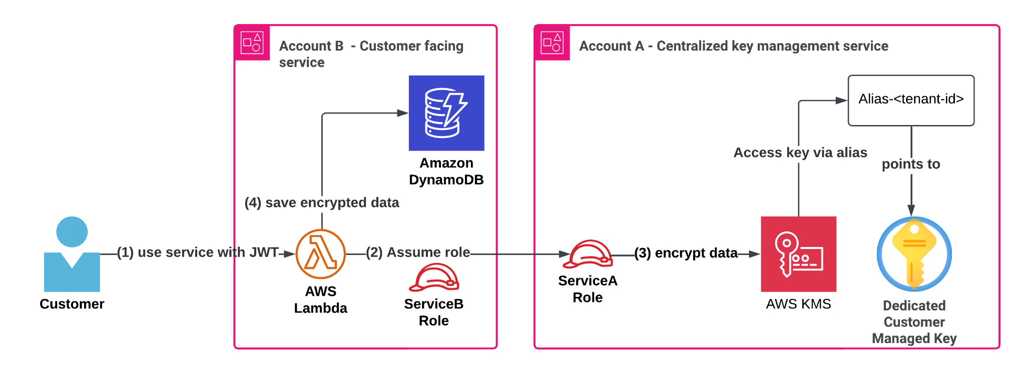
AWS Transfer Family

AWS Transfer Family is a managed file transfer service for SFTP, FTPS, and AS2 protocols. It integrates directly with Amazon Simple Storage Service (Amazon S3) for storage and supports custom identity providers for authentication through Amazon API Gateway and AWS Lambda.

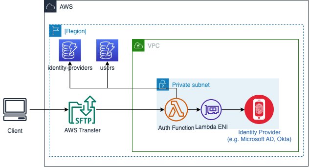
As shown in Figure 1, when a user initiates a file transfer, Transfer Family authenticates them through the configured identity provider using API Gateway and Lambda. After authentication succeeds, the service maps the user to an AWS Identity and Access Management (IAM) role that defines their S3 bucket access permissions. The service encrypts data in transit using TLS 1.2 and data at rest using S3 server-side encryption.

Figure 1: AWS Transfer Family architecture

Figure 1: AWS Transfer Family architecture

Transfer Family automatically handles scaling from zero to thousands of concurrent users, manages high availability across Availability Zones, and minimizes infrastructure management. It records detailed metrics and logs in Amazon CloudWatch for monitoring and auditing, supporting compliance requirements with activity tracking.

It’s important to note that Transfer Family also offers service-managed authentication. This simpler setup stores user credentials (passwords or SSH keys) directly in Transfer Family, minimizing the need for external identity providers. Service-managed authentication is best suited if you have a small number of users or no existing identity management system, or when you want to have a disconnected identity system and don’t want to give external partners an account in your identity provider system.

Pros

One of the biggest advantages of Transfer Family is how it provides the reliability and scalability of Amazon S3 for storing your data, while keeping that data available to existing client applications and workflows. The service integrates with existing authentication systems through custom identity providers, while maintaining security through IAM policies. Its auto-scaling capabilities handle variable workloads, from occasional transfers to high-volume scenarios.

Transfer Family also offers detailed CloudWatch logging and audit trails for file transfer activities, which should be sufficient for most logging and audit needs. It encrypts data in transit using TLS 1.2 and at rest using Amazon S3 server-side encryption. You can implement fine-grained access controls through IAM roles and integrate with AWS Organizations for multi-account management. The service supports VPC endpoints for secure internal access and custom domain names for branded endpoints.

Because data is stored in S3, some of your requirements will be fulfilled by configuring S3, not the Transfer Family services. Data retention (for example, avoiding deletion and scheduling deletion) is achieved through S3 Object Lock and S3 Lifecycle Events.

Cons

The pricing structure of Transfer Family includes $0.30 per hour for each protocol you enable and data transfer fees based on data volume. There can be additional charges for custom domain names. If you use VPC endpoints for secure internal access to Amazon S3, there will also be VPC data charges. If you have high-volume transfers or multiple endpoints across AWS Regions, you will face increased costs. Because the data ultimately lives in S3; S3 storage and request pricing applies as well.

Custom identity provider implementations (such as SAML or OAuth) add latency to authentication processes, affecting transfer initiation times. This authentication process requires additional configuration and introduces extra steps and latency during transfer initiation compared to service-managed authentication.

The Regional nature of Transfer Family means you must choose between deploying in a single Region (simpler management but potential latency for global users) or multiple Regions (better performance but higher costs at $0.30 per protocol per hour per Region). Multi-Region can serve as a disaster recovery strategy or when Regional data isolation is needed.

Transfer Family web apps

Transfer Family web apps provide browser-based access to Amazon S3, enabling users to upload and download files through a web interface. With the web apps, you can create a branded, secure, and highly available portal for your users to browse, upload, and download data in S3. Web apps are built using Storage Browser for S3 and offer the same user functionalities in a fully managed offering without having to write code or host your own application.

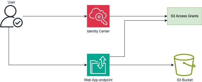
When a user accesses the web application, authentication occurs through AWS IAM Identity Center, and S3 Access Grants determine their permissions to specific S3 buckets or prefixes. The access grant permissions can be either read-only or read and write. After authentication succeeds, users can upload or download files directly through the web interface. The service uses Amazon CloudFront for content delivery and implements SSL/TLS encryption for data transfers, while S3 provides server-side encryption for data at rest. Figure 2 shows a simplified Transfer Family web app architecture.

Figure 2: Simplified Transfer Family web app architecture

Figure 2: Simplified Transfer Family web app architecture

The web application automatically scales to accommodate varying numbers of users and provides high availability through the CloudFront global edge network. It minimizes the need for custom web application development and provides logging through AWS CloudTrail and CloudWatch. You can customize the user experience by implementing custom domains through CloudFront distributions.

Transfer Family web apps support multiple authentication methods, with IAM Identity Center being one of the primary options. While Identity Center provides simplified user management and integration with existing identity providers. It also provides useful mechanisms such as multi-factor authentication (MFA), strong password policies, and resetting lost passwords. It’s not the only authentication method available; you can also use custom identity providers for authentication, providing flexibility in how you manage user access to the web application.

Pros

Transfer Family web apps minimize the need to build and maintain custom web interfaces for Amazon S3 file sharing. It provides seamless integration with IAM Identity Center for user management and authentication, enabling you to use existing identity providers. The service offers fine-grained access control through S3 Access Grants, allowing precise permission management at the bucket and prefix level. Its integration with CloudFront provides global availability and enhanced performance, while CloudTrail logging offers audit capabilities.

The service provides robust security features including SSL/TLS encryption, CORS policy management, and optional integration with AWS WAF for protection against bots, web scrapers, DDoS events, and more. You can implement custom domains for branded experiences and use CloudFront security features including DDoS protection using AWS Shield. The web interface offers intuitive file management capabilities without requiring client software or that users have technical expertise.

Cons

Transfer Family web apps require using IAM Identity Center, which might require additional setup and configuration if you’re not currently using this service. The web interface currently requires the Identity Center identities to live in the same AWS account as the S3 buckets. That might create design challenges if you want to keep identities in one AWS account and data storage in another. Implementation requires careful cross-origin resource sharing (CORS) configuration for each S3 bucket.

The service incurs costs for both Transfer Family and associated services, including CloudFront distribution and data transfer fees. Custom domain implementation requires additional configuration and SSL certificate management through AWS Certificate Manager (ACM). The web interface is well suited for humans to upload or download, but it’s not as good for automated workflows that transfer files from machine to machine. You must carefully manage user assignments and access grants to maintain security, adding administrative overhead.

S3 pre-signed URLs

Amazon S3 pre-signed URLs enable secure, time-limited access to objects in S3 without requiring the file recipient to have an identity in your identity systems. The URLs are generated using the AWS SDK or AWS Command Line Interface (AWS CLI), granting specific permissions (GET, PUT) that are valid for up to seven days. When accessing files, S3 validates the cryptographically signed parameters in these URLs before permitting access to objects. This provides a direct method for secure file sharing through HTTPS endpoints.

The solution requires only an S3 bucket and appropriate IAM permissions for URL generation. S3 handles the authentication of the pre-signed URL parameters and manages access to objects. File transfers occur directly between users and S3 through HTTPS endpoints, with the pre-signed URL controlling the access patterns.

Amazon S3 provides security features including server-side encryption, access logging, and CloudTrail integration. The security of pre-signed URLs is primarily managed through expiration times and specific operation permissions defined during URL generation.

Pros

Amazon S3 pre-signed URLs follow a straightforward pay-per-use pricing model, charging only for S3 storage, requests, and data transfers. For example, if you create pre-signed URLs but the object isn’t actually downloaded, you pay storage costs as usual, but you don’t pay transfer costs. The solution uses the native scalability of S3 to handle varying numbers of concurrent users without additional infrastructure. you can implement granular access controls through URL expiration times and specific operation permissions (GET, PUT, DELETE).

Access is controlled through URL expiration enforcement. Amazon S3 server access logging and CloudTrail integration enable audit capabilities. The solution’s simplicity makes it ideal for basic file sharing needs while maintaining security and scalability.

Cons

A pre-signed URL can be used by anyone who has access to the URL. That’s the goal of this design: You don’t need to have an identity for the user. Pre-signed URLs can be reused an unlimited number of times until they expire. To improve security, short expiration times can limit the potential for URL re-use. Shorter expiration times, however, require the recipient to download the file soon after the URL is created.

When implementing this solution, you should establish processes for secure URL generation and distribution. Set your URL expiration times based on realistic expectations about how quickly your recipients will download the files. A web or mobile app where the user selects a link to download something (such as a document, an image, a data file) and they expect the download to start immediately is a good candidate for this design.

The solution works with files up to 5 GB for single operations. To share a file larger than 5 GB, you must split the file into multiple parts, issue multiple pre-signed URLs, and then the recipient must download all the parts and join the parts together correctly. This isn’t a good solution for sharing large files. Also, distributing large files as a single download can be difficult if the recipient doesn’t have good connectivity. Amazon S3 can start an object download from the middle of the object, but selecting a pre-signed URL cannot. So, if the recipient transfers 1 GB out of a 2 GB download, and then their connection is disrupted, they cannot pick up where they left off. They will restart from the beginning, which is undesirable. Overall, this design is unsuitable for transmitting large files over unreliable internet connections.

You should enable appropriate monitoring through Amazon S3 access logs and CloudTrail to track usage patterns and meet security compliance.

This solution is particularly effective if you’re seeking straightforward, secure file sharing capabilities where the files are small enough to download in one request, and where you have a secure mechanism to share the download URLs.

Serverless web application with S3 presigned URLs

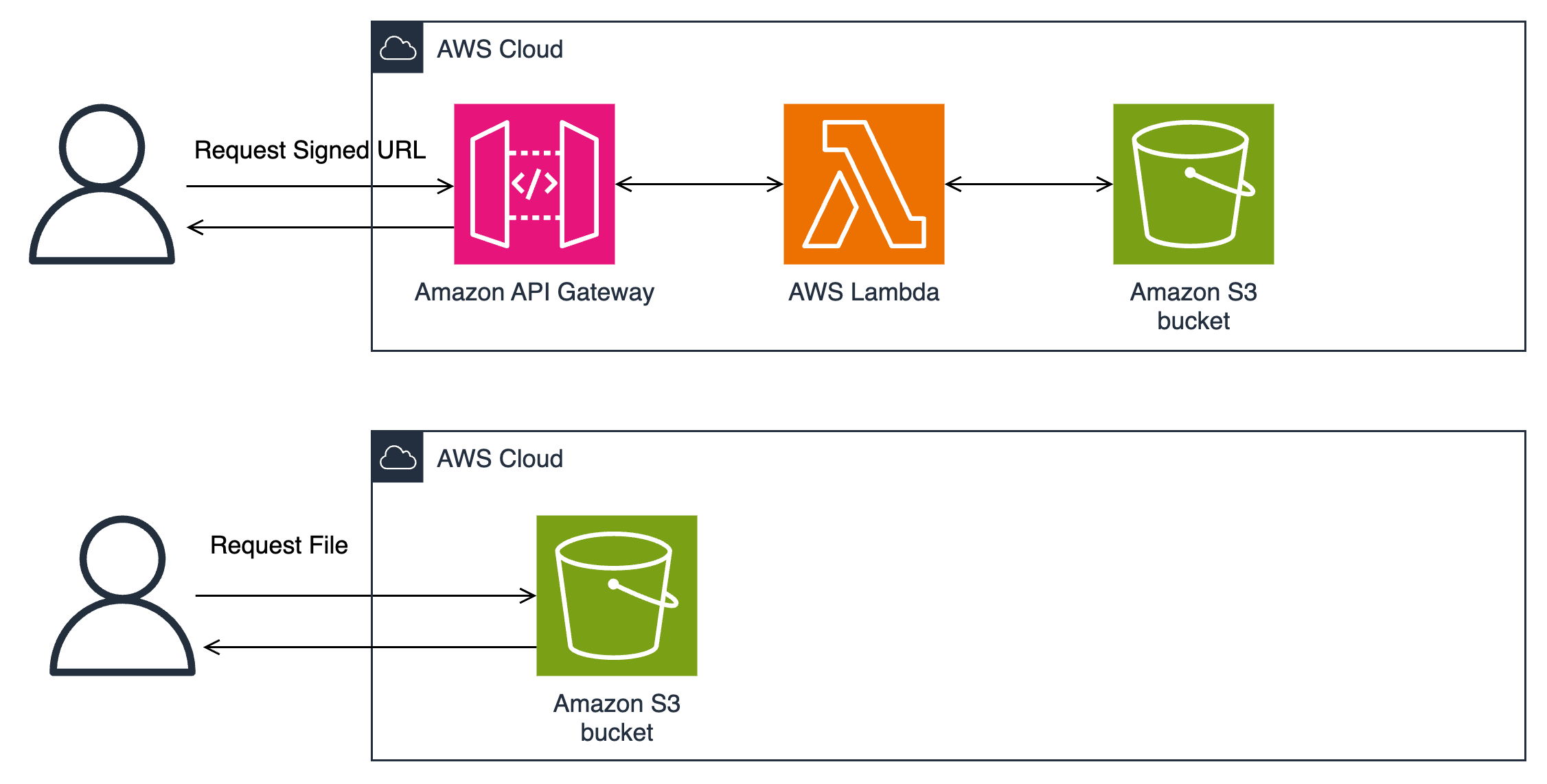
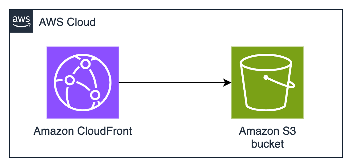
Amazon S3 presigned URLs combined with a custom web application enable secure, time-limited access to S3 objects. The application generates URLs that grant specific S3 permissions (GET, PUT) for between one minute and seven days. When requesting file access, the application authenticates users and generates presigned URLs using the AWS SDK with defined permissions and expiration times.

The web application uses API Gateway and Lambda functions for authentication and URL generation. Amazon S3 validates the cryptographically signed parameters in these URLs before permitting access to objects. File transfers occur directly between users and S3 through HTTPS endpoints, with the application controlling the access patterns. The architecture is shown in Figure 3.

Figure 3: Amazon S3 pre-signed URLs architecture

Figure 3: Amazon S3 pre-signed URLs architecture

The web application can implement security controls including request logging, rate limiting (requests per second), and authentication workflows. CloudWatch logs record API access patterns and Lambda execution metrics, while Amazon S3 access logging records object-level operations.

Pros

Amazon S3 presigned URLs follow a pay-per-use pricing model. This solution charges only for API Gateway requests, Lambda executions, and S3 operations performed. The serverless architecture scales automatically from zero to thousands of concurrent users without infrastructure management. You can implement custom security controls and business logic for specific access requirements through API Gateway authorizers (using custom identity solutions or Amazon Cognito) and Lambda functions.

The solution enforces security through URL expiration (maximum seven days), IAM policies restricting URL generation permissions, and HTTPS encryption for data transfers. Custom authentication workflows integrate with existing identity providers (SAML, OIDC). Additional security features include IP-based restrictions, required request headers, and request validation through AWS WAF. This solution would be good, for example, if you have a variety of files or a variety of buckets and you’re trying to build a unified front-end where people can download various files without knowing which bucket the files are stored in or what URL expiration time is appropriate. You can configure the frontend to look at tags on objects, tags on buckets, object names, or another attribute that fits your use case, and then choose a URL expiration time based on that attribute. For example, objects from buckets tagged Data Classification: Restricted might expire after 1 minute, whereas objects from buckets tagged Data Classification: Public might be valid for 7 days.

Cons

Building a custom web application requires developing and maintaining the code for URL generation, authentication, and error handling logic. The application must track URL expiration times and implement mechanisms that permit retries for failed transfers. Monitoring systems must track URL usage, detect abuse patterns, and send alerts for security violations through CloudWatch metrics and logs.

One limitation of this solution is the 10 MB size limit imposed by API Gateway. This affects how your application handles file uploads and downloads. For uploads, files under 10 MB can be uploaded directly through API Gateway. Larger files require implementing multipart uploads, where the client splits the file into chunks and sends each chunk separately. For downloads, files under 10 MB can be downloaded directly through API Gateway but for larger files, your application should generate a pre-signed URL for direct Amazon S3 access, bypassing API Gateway.

URL generation errors or misconfigured IAM permissions can expose objects to unauthorized access. The HTTPS-only protocol limits integration with SFTP and FTPS clients. Files larger than 5 GB require multipart upload implementation, and network interruptions need custom resume logic. This design will incur some extra charges if the number of file transfers are the millions. Lambda functions cost $0.20 per million requests, and API Gateway costs $1.00 per million requests. Analyze your expected access patterns to determine whether these extra costs will be significant and if they’re worth the additional flexibility of custom transfer logic.

Decision matrix: When to use each solution

The following table summarizes the characteristics of the solutions presented in the two parts of this post. See Part 2 for full descriptions of the solutions not covered in Part 1.

Characteristics Transfer Family Transfer Family web app S3 pre-signed URLs (Direct) Serverless web application with S3 pre-signed URL CloudFront signed URLs (Part 2) VPC endpoint service (Part 2) S3 Object Lambda (Part 2)
Protocol support SFTP, FTPS, and AS2 HTTPS (web-based) HTTPS HTTPS HTTPS with CDN A TCP-based protocol HTTPS
Global distribution Global endpoint support CloudFront integration Global S3 access Global S3 access Global edge network acceleration Direct AWS backbone access Global S3 access with Regional endpoints
Pricing model Hourly service rate and usage Pay per file operation Pay-per-request Pay-per-request and application costs Pay-per-request with caching savings Hourly endpoint rate and usage No additional charge for access points; standard S3 request pricing applies
Content processing Direct S3 integration Built-in web interface Direct S3 access Custom app processing Edge-based file processing Access files through private network Direct S3 access with customized permissions per access point
Authentication options Custom IdP and service-managed IAM Identity Center IAM Custom authentication possible IAM, custom authentication, and edge validation VPC security controls and custom authentication IAM policies, VPC endpoint policies, resource-based policies
Upload capabilities Unlimited file size Web interface upload Up to 5 GB direct and multipart for larger Up to 10 MB using API Gateway Optimized for global ingestion Unlimited file size over private connection Same as standard S3
Download capabilities Unlimited file size Browser-based downloads Up to 5 GB using a single URL Up to 10 MB using API Gateway Accelerated downloads using global edge locations Unlimited file size over private connection Same as standard S3 with customized access controls
Example use cases
  • Enterprise file transfer systems
  • B2B data exchange
  • Compliance-focused transfers
  • Browser-based file sharing
  • Internal document management
  • Client portals
  • Simple direct S3 access
  • Temporary file sharing
  • Mobile app backend
  • Custom file sharing systems
  • Integrated web applications
  • Enhanced S3 access control
  • Global content delivery
  • Media distribution
  • Web application assets
  • Private network transfers
  • Custom protocol support
  • Secure enterprise data exchange
  • Simplified data access management at scale
  • Multi-application access to shared datasets
  • VPC-restricted data access

The following list gives you a quick overview of the strengths of each solution presented in the two parts of this post.

  • Transfer Family is the optimal choice for organizations that require legacy file transfer protocols such as SFTP, FTPS, or AS2 protocols, and you must integrate with existing authentication systems. It’s ideal for scenarios with strict compliance and audit requirements, where operational overhead needs to be minimized. While the solution comes with higher costs because of its managed service nature, it’s often the lowest-friction option to support existing enterprise use cases that depend on these protocols.
  • Transfer Family web apps suit organizations that need browser-based file sharing without custom development. They integrate with IAM Identity Center for user authentication and uses Amazon S3 Access Grants for permission management. The solution works well for internal document sharing, client portals, and scenarios requiring a branded web interface. While limited to web browser access, they provide built-in features like MFA and password management without infrastructure maintenance.
  • Amazon S3 pre-signed URLs excel in scenarios where simplicity, cost-effectiveness, and temporary access are key requirements. This solution is ideal if you’re seeking a straightforward file sharing mechanism without the need for custom application development or additional infrastructure. This approach shines in environments that require a quick implementation of secure file sharing and cost-effective solutions with minimal overhead.
  • Serverless web application with S3 presigned URLs best serves scenarios where cost optimization is paramount and the HTTPS protocol meets your requirements. This solution shines in environments that need simple, direct file sharing capabilities with quick implementation timelines. It’s particularly effective for moderate usage patterns where serverless architecture can provide cost benefits. The solution’s simplicity makes it ideal for web applications and scenarios where complex file transfer protocols aren’t necessary, though careful consideration must be given to its 10 MB file size limitation for single operations using API Gateway.

In Part 2:

  • CloudFront signed URLs excel in situations that demand global content distribution with high performance requirements. This solution is the clear choice when your architecture needs built-in DDoS protection and performance optimization through caching. It’s particularly valuable when content delivery speed is crucial and you require security at edge locations. The solution’s global reach and caching capabilities make it cost-effective for large-scale content distribution, though it’s primarily optimized for download scenarios rather than uploads.
  • Amazon VPC endpoint service is the preferred choice if you require complete network isolation and maximum security. This solution is ideal when you need support for custom protocols while maintaining private network connectivity. It’s particularly suitable for scenarios with extremely high security requirements and when you have the necessary resources to managed networking configurations. While this solution requires significant expertise and investment, it provides the highest level of security and control for sensitive data transfers.
  • S3 Access Points are best suited for scenarios that require simplified data access management at scale. This solution excels when you need to provide different access patterns to the same underlying data for multiple applications or user groups. It’s ideal if you prefer a structured approach to permissions and need network-level access controls. While primarily focused on simplifying complex access scenarios without modifying bucket policies, it offers unique capabilities for VPC-restricted access and granular permissions management, though subject to certain service limits and configuration requirements.

Conclusion

In this first part of a two-part post, you’ve learned about multiple solutions for secure file sharing using AWS services and the pros and cons of each. You can find additional options in Part 2. The optimal solution depends on your specific organizational requirements, technical capabilities, and budget constraints. You don’t have to choose just one option, you can implement multiple solutions to address different use cases, creating a file sharing strategy that balances security, cost, and operational efficiency.

Additional resources:

If you have feedback about this post, submit comments in the Comments section below.

Swapnil Singh

Swapnil Singh

Swapnil is a Senior Solutions Architect for AWS World Wide Public Sector. As a Product Acceleration Solutions Architect at AWS, she currently works with GovTech customers to ideate, design, validate, and launch products using cloud-native technologies and modern development practices.

Sumit Bhati

Sumit Bhati

Sumit is a Senior Customer Solutions Manager at AWS, specializing in expediting the cloud journey for enterprise customers. Sumit is dedicated to assisting customers through every phase of their cloud adoption, from accelerating migrations to modernizing workloads and facilitating the integration of innovative practices.