All posts by Julien Simon

Scaling Ad Verification with Machine Learning and AWS Inferentia

Post Syndicated from Julien Simon original https://aws.amazon.com/blogs/aws/scaling-ad-verification-with-machine-learning-and-aws-inferentia/

Amazon Advertising helps companies build their brand and connect with shoppers, through ads shown both within and beyond Amazon’s store, including websites, apps, and streaming TV content in more than 15 countries. Businesses or brands of all sizes including registered sellers, vendors, book vendors, Kindle Direct Publishing (KDP) authors, app developers, and agencies on Amazon marketplaces can upload their own ad creatives, which can include images, video, audio, and of course products sold on Amazon. To promote an accurate, safe, and pleasant shopping experience, these ads must comply with content guidelines.

Here’s a simple example. Can you figure out why two of the following ads would not be compliant?

Amazon Ads

The ad in the center doesn’t feature the product in context. It also shows the same product multiple times. The ad on the right looks much better, but it contains text, which is not allowed for this ad format.

New ad creatives come in many sizes, shapes, and languages, and at very large scale. Assuming it would even be possible, verifying them manually would be a complex, slow, and error-prone process. Machine learning (ML) to the rescue!

Using Machine Learning to Verify Ad Creatives
Each ad must be evaluated against many rules, which no single model could reasonably learn. In fact, it takes many models to check ad properties, for example:

  • Media-specific models that analyze images, video, audio, and text that describe the advertised products.
  • Content-specific models that detect headlines, text, backgrounds, and objects.
  • Language-specific models that validate syntax and grammar, and flag unapproved language.

Some of these capabilities are readily available in AWS AI services. For example, Amazon Advertising teams use Amazon Rekognition to extract metadata information from images and videos.

Other capabilities require custom models trained on in-house datasets. For this purpose, Amazon teams labeled large ad datasets with Amazon SageMaker Ground Truth, using a combination of manual labeling, and automatic labeling with active learning. Using these datasets, teams then used Amazon SageMaker to train models, and deploy them automatically on real-time prediction endpoints with the AWS Cloud Development Kit (AWS CDK) and Amazon SageMaker Pipelines.

When a business uploads a new ad, relevant models are invoked simultaneously to process specific ad components, extract signals, and output a quality score. All scores are then consolidated, and sent to a final model that predicts whether the ad should be manually reviewed.

Thanks to this process, most new ads can be verified and published automatically, which means businesses can quickly promote their brand and products, and Amazon can maintain a high-quality shopping experience.

However, faced with a growing number of more complex models, Amazon Advertising teams started to look for a solution that could increase prediction throughput while reducing costs. They found it in AWS Inferentia.

What is AWS Inferentia?
Available in Amazon EC2 Inf1 instances, AWS Inferentia is a custom chip built by AWS to accelerate ML inference workloads, and optimize their cost. Each AWS Inferentia chip contains four NeuronCores. Each NeuronCore implements a high-performance systolic array matrix multiply engine, which massively speeds up typical deep learning operations such as convolution and transformers. NeuronCores are also equipped with a large on-chip cache, which helps to cut down on external memory accesses, reduce latency, and increase throughput.

Thanks to AWS Neuron, a software development kit for ML inference, AWS Inferentia can be used natively from ML frameworks like TensorFlow, PyTorch, and Apache MXNet. It consists of a compiler, runtime, and profiling tools that enable you to run high-performance and low latency inference. For many trained models, compilation is a one-liner with the Neuron SDK, not requiring any additional application code changes. The result is a high performance inference deployment, that can easily scale while keeping costs under control. You’ll find many examples in the Neuron documentation. Alternatively, thanks to Amazon SageMaker Neo, you can also compile models directly in SageMaker.

Scaling Ad Verification with AWS Inferentia
Amazon Advertising teams started compiling their models for Inferentia, and deploying them on SageMaker endpoints powered by Inf1 instances. They compared the Inf1 endpoints to the GPU endpoints they had been using so far. They found that large deep learning models like BERT run more effectively on Inferentia, which decreases latency by 30%, and reduces costs by 71%. A few months ago, ML teams working on Amazon Alexa came to the same conclusions.

What about prediction quality? GPU models are typically trained with single-precision floating-point data (FP32). Inferentia uses the shorter FP16, BF16, and INT8 data types, which can create slight differences in predicted output. Running both GPU and Inferentia models in parallel, teams analyzed probability distributions, tweaked prediction thresholds for their Inferentia models, and made sure that these models would predict ads just like GPU models did. You can learn more about these techniques in the Performance Tuning section of the documentation.

With these final adjustments out of the way, the Amazon Advertising teams started phasing out GPU models. All text data is now predicted on Inferentia, and the migration of computer vision pipelines is in progress.

AWS Customers Are Successful with AWS Inferentia
In addition to Amazon teams, customers also report very nice results on scaling and optimizing their ML workloads with Inferentia.

Binghui Ouyang, Senior Data Scientist at Autodesk: “Autodesk is advancing the cognitive technology of our AI-powered virtual assistant, Autodesk Virtual Agent (AVA) by using Inferentia. AVA answers over 100,000 customer questions per month by applying natural language understanding (NLU) and deep learning techniques to extract the context, intent, and meaning behind inquiries. Piloting Inferentia, we are able to obtain a 4.9x higher throughput over G4dn for our NLU models, and look forward to running more workloads on the Inferentia-based Inf1 instances.

Paul Fryzel, Principal Engineer, AI Infrastructure at Condé Nast: “Condé Nast’s global portfolio encompasses over 20 leading media brands, including Wired, Vogue, and Vanity Fair. Within a few weeks, our team was able to integrate our recommendation engine with AWS Inferentia chips. This union enables multiple runtime optimizations for state-of-the-art natural language models on SageMaker’s Inf1 instances. As a result, we observed a 72% reduction in cost than the previously deployed GPU instances.”

Getting Started
You can get started with Inferentia and Inf1 instances today, either on Amazon SageMaker or with the Neuron SDK. This self-paced workshop walks you through both options.

Give it a try, and let us know what you think. As always, we look forward to your feedback. You can send it through your usual AWS Support contacts, post it on the AWS Forum for SageMaker, or on the Neuron SDK Github repository.

– Julien

Decoding the Social Effects Of Media with Machine Learning

Post Syndicated from Julien Simon original https://aws.amazon.com/blogs/aws/decoding-the-social-effects-of-media-with-machine-learning/

What if media were optimized to benefit people? This thought-provoking question is at the core of Harmony Labs‘ mission. A nonprofit organization headquartered in New York City, Harmony Labs strives to better understand the impact of media on society, and build communities and tools to reform and transform media systems.

Brian WaniewskiAs Brian Wanieswki, Executive Director at Harmony Labs puts it: “The media systems that we have now, for better or worse, have become outrage machines and sorting machines that put people into groups of like minds. The business incentive structures of these systems are such that the more outrage there is, the more profit there is. Political events across the world in recent years have borne out what these media systems produce, and it’s really pretty toxic, and pretty hard to get anything done within. There are all kinds of natural divisions between people, but these media systems tend to reinforce these divisions. So, the first question that we’re asking is, What’s the scope of this problem? And then, What can we do to solve it?”

Harmony Labs use data science and machine learning to answer these questions. Starting from user surveys and media data, they developed advanced natural language processing pipelines that can identify how social issues are represented in media, how they are consumed by different audiences, and what kind of influence that consumption has.

So how do you get that data in first place? Brian says: “All the media data that we need lives inside private companies. We knew that data sharing would be central to our mission, and this is why we’re structured as a nonprofit. We are working in the public’s interest in a non-partisan way. We’ve done big data sharing deals with large companies, as well as startups scraping different corners of the media ecosystem that we’re interested in: internet TV, internet radio, and so on. We have about 10 data partners at the moment, and we’re always looking to expand.

Thanks to their data partners, Harmony Labs has collected over 50 Terabytes of diverse media: TV, web, mobile, song lyrics, closed captions, social media, and more. This definitely fits the definition of big data (volume, velocity and variety). Working with languages like Golang, Python and R, the Harmony Labs data science and engineering teams rely on AWS services such as Amazon Aurora, Amazon Athena, AWS Glue and Amazon Elastic Kubernetes Service (EKS) to build their data ingestion and processing workflows.

Laura EdelsonOnce the data is in-house, Harmony Labs make it safe, secure, and accessible to a network of academic researchers who use it to investigate the influence of media systems on politics, society, and culture. Laura Edelson is one of these researchers. A Ph.D. Candidate in Computer Science at NYU’s Tandon School of Engineering, she studies online political communication and develops methods to identify inauthentic content and activity. Harmony Labs supported her on the Ad Observatory project, an exploration of political ads on Facebook.

Harmony Labs also work on their own projects, such as the Narrative Observatory. “A narrative is a story pattern that recurs across different kinds of stories and media. You’ll find them in song lyrics, TV shows, news articles, and more“, says Brian. The Narrative Observatory helps identify narratives on particular topics and track them over long periods of time, and across different media types.

With initial funding from the Bill & Melinda Gates Foundation, Harmony Labs studied narratives linked to the topic of poverty and economic mobility in the United States. Collecting millions of documents (online news, social media, music), they first identified the main narratives present in media. Then, using segmentation techniques, behavioral data on over 50,000 Americans and surveys, Harmony Labs defined four audiences, as well as their dominant narrative, their core values, and their views on specific social issues. Finally, Harmony Labs studied how each audience consumed narratives.

To enable funders, partners, and media companies to gain a deeper understanding of the cultural spaces their audiences occupy, they built a fascinating website, obiaudiences.org, where you can pick an audience and view the associated media feed. In other words, you can literally see the world in someone else’s eyes: what issues they care most about, what media they read most, and so on. This helps to understand the perceptions that different people have on certain issues, and as Brian puts it: “If you’re trying to reach people, it’s important to understand the media world they inhabit, and what can be actually relevant to that world.

Narrative Observatory

Recently, Harmony Labs led a project funded by the Mozilla Foundation on defining a healthy narrative for artificial intelligence (AI). Studying the TV consumption habits of over 80,000 US adults, and connecting them with closed captioned transcripts and ads, they identified and named the main media narratives on AI. Each narrative includes a definition of AI, the emotion that it creates in people, and whether they think that AI will lead to a happy or an unhappy ending.

Harmony Labs identified four main narratives on AI. Two are extremely negative and fear-inducing. “Tool of Tyranny” says that AI will be used by governments to oppress people. “Robot Overlords” says that we’ll never be able to control AI, and it will end up ruling us. At the other end of the spectrum, the “Wishes Granted” narrative is extremely positive: sure, we don’t understand AI, but it’s a magic wand that will solve all our issues. The last narrative, “Augmented Intelligence”, is more balanced: yes, AI is a great opportunity to improve our daily lives, but it’s also capable of being unfair and even dangerous. We are responsible for designing it, controlling it, and making sure it’s used to help us, not to hurt us.

Harmony Labs found that the “Wishes Granted” narrative was the most prominent (67%). It shines a positive light on AI, but its naive and over-optimistic vision can hide the legitimate questions that AI raises. Still, it’s a good starting point to engage audiences, educate them with the “Augmented Intelligence” narrative, and increase their awareness on both opportunities and challenges.

Closing this post, I’m wondering which AI narrative I’ve actually promoted here, willingly or not! What do you think? One thing is certain: Harmony Labs is using AI to help us understand how media influences us every day, and how we can create a more democratic society. This is important work, and we’re humbled that they picked AWS to help them reach their goals.

For more information on Harmony Labs, please visit harmonylabs.org and harmonylabs.medium.com.

– Julien

Extract Insights From Customer Conversations with Amazon Transcribe Call Analytics

Post Syndicated from Julien Simon original https://aws.amazon.com/blogs/aws/extract-insights-from-customer-conversations-with-amazon-transcribe-call-analytics/

In 2017, we launched Amazon Transcribe, an automatic speech recognition (ASR) service that makes it easy to add speech-to-text capabilities to any application. Today, I’m very happy to announce the availability of Amazon Transcribe Call Analytics, a new feature that lets you easily extract valuable insights from customer conversations with a single API call.

Each discussion with potential or existing customers is an opportunity to learn about their needs and expectations. For example, it’s important for customer service teams to figure out the main reasons why customers are calling them, and measure customer satisfaction during these calls. Likewise, salespeople try to gauge customer interest, and their reaction to a particular sales pitch.

Thus, many customers and partners would like to add call analytics capabilities in different applications, regardless of their contact center provider. They often need to analyze more than phone calls, for example web-based audio and video calls. So far, they’ve typically done this by stitching AI services and dedicated ML models together, and they’ve asked us for a simpler solution.

We got to work and built Amazon Transcribe Call Analytics, a new addition to Transcribe and a key enhancement to AWS Contact Center Intelligence. If you can’t wait to try it, feel free to jump now to the AWS console. If you’d like to learn more, read on!

Introducing Amazon Transcribe Call Analytics
Based on ASR implemented in Transcribe, Transcribe Call Analytics adds natural language processing (NLP) capabilities specifically trained on customer calls, and optimized to provide highly accurate call transcripts and actionable insights. With a simple API call, developers can now easily add call analytics to any application, and extract customer insights from conversations without having to build AI pipelines and train custom ML models.

Key features of Transcribe Call Analytics include:

  • Timestamped turn-by-turn call transcription in 21 languages.
  • Issue detection, which picks up the shortest set of contiguous words in a conversation turn that represents the reason why the customer is calling. This works out of the box without any configuration or training.
  • Call categorization based on conversational characteristics:
    • Matching specific words and phrases,
    • Detecting non-talk time,
    • Detecting interruptions,
    • Analyzing sentiment for the customer and the agent.
  • Call characteristics such as:
    • How quickly and loudly a customer or agent are speaking,
    • Detecting non-talk time,
    • Detecting interruptions.
  • Redaction of sensitive data from the text transcript and the corresponding audio file.

For example, you can create rules to flag calls where customers interrupt the agent, exhibit negative sentiment, and say “I want to speak with the manager”. These calls certainly did not go well, and are worth analyzing in detail! You can also look for calls where agents don’t use pre-defined greetings (“Welcome to ACME Support, how can I help you today?”) within the first 15 seconds, to measure script compliance and help supervisors identify agent coaching opportunities. Another popular scenario is to create rules that flag mentions of your specific products and services (“Your ACME Turbo 2000 vacuum cleaner isn’t working like it should”), in order to pick up any emerging trends you’d need to be aware of.

Last but not least, you can further process the text transcript with other AI services such as Amazon Translate, or with custom NLP models built with Amazon SageMaker.

Now, let’s do a quick demo.

Extracting Insights with Amazon Transcribe Call Analytics
Here’s a fictitious support call, where a lady calls her bank to report that she’s lost her credit and debit cards. The sound file is a stereo WAV file (16-bit, 8KHz).

Transcribe Call Analytics requires that the agent and the customer are recorded in their own channel. We’ll also need to tell which is the agent channel. In a stereo file, the left channel is usually the first channel (channel #0), and the right channel is the second one (channel #1). This is the case for this call.

If you’re not sure which is which, you can easily use the versatile ffmpeg open source tool to extract each channel to a separate audio file.

$ ffmpeg -i demo-call.wav -map_channel 0.0.0 channel0.wav -map_channel 0.0.1 channel1.wav

You can use the same technique to extract audio channels from other file types, such as video files, and recombine them to a stereo audio file. You’ll find more information in the ffmpeg documentation.

Now that I’m sure that the agent is in channel #1, I use the AWS CLI to upload the audio file to an S3 bucket.

$ aws s3 cp launch-call.wav s3://jsimon-transcribe-useast1/demo-call.wav --region us-east-1

Opening the Transcribe Call Analytics console, I see that call category templates are available.

Call categories

I decide to create one for supervisor escalations. Then, with a couple of clicks, I create a custom call category named welcome-message, to check if the agent starts the call with an appropriate welcome. I could add several phrases to check for if needed. We recommend that you use short sentences to minimize the chance of filler words popping up (‘hmm’, ‘err’, and so on).

Call category

Then, I create a call analytics job using the general model available in Transcribe. I also enable automatic language detection.

Creating a job

Then, I define the location of the audio file in S3, flagging channel #1 as the agent channel.

Creating a job

I decide to store the transcript in the default S3 bucket created by Transcribe in my account. I could also use my own bucket if needed. Then, I pick an AWS Identity and Access Management (IAM) role with sufficient permissions, and I launch the job.

A minute later or so, the job is complete. The console contains a preview of the text transcript, as well as a link to the full JSON transcript.

Viewing the transcript

As the agent used the proper welcome sentence in the first 15 seconds, the call is tagged with the category I created earlier.

Call categories

Downloading the JSON transcript, each sentence in the conversation is enriched with metadata on per-word loudness, measured on a 0-100 range with 100 being extremely loud. Here’s the first sentence:

"BeginOffsetMillis":440,"EndOffsetMillis":4960,
"Sentiment":"NEUTRAL",
"ParticipantRole":"AGENT",
"LoudnessScores":[78.68,80.4,81.91,78.95,82.34],
"Content":"Hello and thank you for calling the bank. This is Ashley speaking, how may I help you today?"

Looking at the next sentence, I see that Transcribe Call Analytics automatically detected what the customer issue is. The corresponding text is in bold:

"Content": "Hi um uh you just need to cancel my card. Um I have a debit card and a credit card.",
"IssuesDetected":[{"UnredactedCharacterOffsets":{"Begin": 26,"End": 40}}. . .

At the end of the transcript, I see global call statistics (duration, talk time, words per minute, matched categories). Transcribe also gives me overall sentiment information, meaured from -5 (extremely negative) to +5 (extremely positive). I also get a a breakdown in four quarters.

"Sentiment":{"OverallSentiment":{"AGENT":2.6,"CUSTOMER":0.2},
"SentimentByPeriod":{"QUARTER":
{"AGENT":[
{"Score":1.9,"BeginOffsetMillis":0,"EndOffsetMillis":68457},
{"Score":-0.7,"BeginOffsetMillis":68457,"EndOffsetMillis":136915},
{"Score":5.0,"BeginOffsetMillis":136915,"EndOffsetMillis":205372},
{"Score":3.0,"BeginOffsetMillis":205372,"EndOffsetMillis":273830}],
"CUSTOMER":[
{"Score":-1.7,"BeginOffsetMillis":0,"EndOffsetMillis":68165},
{"Score":0.0,"BeginOffsetMillis":68165,"EndOffsetMillis":136330},
{"Score":0.0,"BeginOffsetMillis":136330,"EndOffsetMillis":204495},
{"Score":2.1,"BeginOffsetMillis":204495,"EndOffsetMillis":272660}]}}}

We can see that the customer started the call with negative sentiment, moving quickly to neutral sentiment, and ending the call with positive sentiment. This is a good sign that the call was handled satisfactorily, and that the customer problem was solved.

If you’d like to convert the transcript to a Word document with additional visualizations, my colleague Andrew Kane has built a nice tool and made it available on Github. Here’s a sample report produced by his tool.

Andrew's tool

AWS Customers and Partners Are Using Amazon Transcribe Call Analytics

Ben Rigby, the SVP, Global Head of Product & Engineering, Artificial Intelligence, Automation, and Workforce at Talkdesk told us, “Our customers are processing millions of customer service calls in their contact centers a year and have a critical need to extract actionable conversation insights to ensure positive business outcomes. As an AWS Contact Center Intelligence partner, we further enhanced our call transcription capabilities with Amazon Transcribe. With the launch of Amazon Transcribe Call Analytics, we’re excited to add even more AI capabilities to our Speech Analytics and QM Assist products. These deeper insights can provide agents and supervisors with the data they need to improve the speed and quality of their customer service while boosting workforce productivity.

Praphul Kumar, the Chief Product Officer of SuccessKPI adds, “Amazon Transcribe Call Analytics API enables us to add ML-based capabilities to our platform faster and at a lower cost. This new API removes the need to integrate multiple AI services together and develop custom machine learning models in certain areas. With Transcribe Call Analytics, we will be able to provide conversation insights such as sentiment, non-talk time, and call categories to gauge agent performance. This helps to drive better call outcomes, reduce agent turnover, uncover agent coaching opportunities, and measure call script compliance. Combining AWS services into SuccessKPI’s experience analytics platform was a no brainer. We are looking forward to bringing this valuable capability into the hands of large enterprises and government agencies.

Getting Started
A single API call is all it takes to extract rich insights from your customer conversations. You can start using Amazon Transcribe Call Analytics today in the following regions:

  • US West (Oregon), US East (N. Virginia),
  • Canada (Central),
  • Europe (London), Europe (Frankfurt),
  • Asia Pacific (Mumbai), Asia Pacific (Singapore), Asia Pacific (Seoul), Asia Pacific (Tokyo), Asia Pacific (Sydney).

Please give this new feature a try in the AWS console, and let us know what you think. We always look forward to your feedback! You can send it through your usual AWS Support contacts or post it on the AWS Forum for Amazon Transcribe.

One last thing: if you’re looking for an easy to use omnichannel cloud contact center, you should definitely take a look at Amazon Connect and its ML powered analytics, Contact Lens.

– Julien

Paging Doctor Cloud! Amazon HealthLake Is Now Generally Available

Post Syndicated from Julien Simon original https://aws.amazon.com/blogs/aws/paging-doctor-cloud-amazon-healthlake-is-now-generally-available/

At AWS re:Invent 2020, we previewed Amazon HealthLake, a fully managed, HIPAA-eligible service that allows healthcare and life sciences customers to aggregate their health information from different silos and formats into a structured, centralized AWS data lake, and extract insights from that data with analytics and machine learning (ML). Today, I’m very happy to announce that Amazon HealthLake is generally available to all AWS customers.

The ability to store, transform, and analyze health data quickly and at any scale is critical in driving high-quality health decisions. In their daily practice, doctors need a complete chronological view of patient history to identify the best course of action. During an emergency, giving medical teams the right information at the right time can dramatically improve patient outcomes. Likewise, healthcare and life sciences researchers need high-quality, normalized data that they can analyze and build models with, to identify population health trends or drug trial recipients.

Traditionally, most health data has been locked in unstructured text such as clinical notes, and stored in IT silos. Heterogeneous applications, infrastructure, and data formats have made it difficult for practitioners to access patient data, and extract insights from it. We built Amazon HealthLake to solve that problem.

If you can’t wait to get started, you can jump to the AWS console for Amazon HealthLake now. If you’d like to learn more, read on!

Introducing Amazon HealthLake
Amazon HealthLake is backed by fully-managed AWS infrastructure. You won’t have to procure, provision, or manage a single piece of IT equipment. All you have to do is create a new data store, which only takes a few minutes. Once the data store is ready, you can immediately create, read, update, delete, and query your data. HealthLake exposes a simple REST Application Programming Interface (API) available in the most popular languages, which customers and partners can easily integrate in their business applications.

Security is job zero at AWS. By default, HealthLake encrypts data at rest with AWS Key Management Service (KMS). You can use an AWS-managed key or your own key. KMS is designed so that no one, including AWS employees, can retrieve your plaintext keys from the service. For data in transit, HealthLake uses industry-standard TLS 1.2 encryption end to end.

At launch, HealthLake supports both structured and unstructured text data typically found in clinical notes, lab reports, insurance claims, and so on. The service stores this data in the Fast Healthcare Interoperability Resource (FHIR, pronounced ‘fire’) format, a standard designed to enable exchange of health data. HealthLake is compatible with the latest revision (R4) and currently supports 71 FHIR resource types, with additional resources to follow.

If your data is already in FHIR format, great! If not, you can convert it yourself, or rely on partner solutions available in AWS Marketplace. At launch, HealthLake includes validated connectors for Redox, HealthLX, Diameter Health, and InterSystems applications. They make it easy to convert your HL7v2, CCDA, and flat file data to FHIR, and to upload it to HealthLake.

As data is uploaded, HealthLake uses integrated natural language processing to extract entities present in your documents and stores the corresponding metadata. These entities include anatomy, medical conditions, medication, protected health information, test, treatments, and procedures. They are also matched to industry-standard ICD-10-CM and RxNorm entities.

After you’ve uploaded your data, you can start querying it, by assigning parameter values to FHIR resources and extracted entities. Whether you need to access information on a single patient, or want to export many documents to build a research dataset, all it takes is a single API call.

Let’s do a quick demo.

Querying FHIR Data in Amazon HealthLake
Opening the AWS console for HealthLake, I click on ‘Create a Data Store’. Then, I simply pick a name for my data store, and decide to encrypt it with an AWS managed key. I also tick the box that preloads sample synthetic data, which is a great way to quickly kick the tires of the service without having to upload my own data.

Creating a data store

After a few minutes, the data store is active, and I can send queries to its HTTPS endpoint. In the example below, I look for clinical notes (and clinical notes only) that contain the ICD-CM-10 entity for ‘hypertension’ with a confidence score of 99% or more. Under the hood, the AWS console is sending an HTTP GET request to the endpoint. I highlighted the corresponding query string.

Querying HealthLake

The query runs in seconds. Examining the JSON response in my browser, I see that it contains two documents. For each one, I can see lots of information: when it was created, which organization owns it, who the author is, and more. I can also see that HealthLake has automatically extracted a long list of entities, with names, descriptions, and confidence scores, and added them to the document.

HealthLake entities

The document is attached in the response in base64 format.

HealthLake document

Saving the string to a text file, and decoding it with a command-line tool, I see the following:

Mr Nesser is a 52 year old Caucasian male with an extensive past medical history that includes coronary artery disease , atrial fibrillation , hypertension , hyperlipidemia , presented to North ED with complaints of chills , nausea , acute left flank pain and some numbness in his left leg

This document is spot on. As you can see, it’s really easy to query and retrieve data stored in Amazon HealthLake.

Analyzing Data Stored in Amazon HealthLake
You can export data from HealthLake, store it in an Amazon Simple Storage Service (Amazon S3) bucket and use it for analytics and ML tasks. For example, you could transform your data with AWS Glue, query it with Amazon Athena, and visualize it with Amazon QuickSight. You could also use this data to build, train and deploy ML models on Amazon SageMaker.

The following blog posts show you end-to-end analytics and ML workflows based on data stored in HealthLake:

Last but not least, this self-paced workshop will show you how to import and export data with HealthLake, process it with AWS Glue and Amazon Athena, and build an Amazon QuickSight dashboard.

Now, let’s see what our customers are building with HealthLake.

Customers Are Already Using Amazon HealthLake
Based in Chicago, Rush University Medical Center is an early adopter of HealthLake. They used it to build a public health analytics platform on behalf of the Chicago Department of Public Health. The platform aggregates, combines, and analyzes multi-hospital data related to patient admissions, discharges and transfers, electronic lab reporting, hospital capacity, and clinical care documents for COVID-19 patients who are receiving care in and across Chicago hospitals. 17 of the 32 hospitals in Chicago are currently submitting data, and Rush plans to integrate all 32 hospitals by this summer. You can learn more in this blog post.

Recently, Rush launched another project to identify communities that are most exposed to high blood pressure risks, understand the social determinants of health, and improve healthcare access. For this purpose, they collect all sorts of data, such as clinical notes, ambulatory blood pressure measurements from the community, and Medicare claims data. This data is then ingested it into HealthLake and stored in FHIR format for further analysis.

Dr. Hota

Says Dr. Bala Hota, Vice President and Chief Analytics Officer at Rush University Medical Center: “We don’t have to spend time building extraneous items or reinventing something that already exists. This allows us to move to the analytics phase much quicker. Amazon HealthLake really accelerates the sort of insights that we need to deliver results for the population. We don’t want to be spending all our time building infrastructure. We want to deliver the insights.


Cortica is on a mission to revolutionize healthcare for children with autism and other developmental differences. Today, Cortica use HealthLake to store all patient data in a standardized, secured, and compliant manner. Building ML models with that data, they can track the progress of their patients with sentiment analysis, and they can share with parents the progress that their children are doing on speech development and motor skills. Cortical can also validate the effectiveness of treatment models and optimize medication regimens.

Ernesto DiMarinoErnesto DiMarino, Head of Enterprise Applications and Data at Cortica told us: “In a matter of weeks rather than months, Amazon HealthLake empowered us to create a centralized platform that securely stores patients’ medical history, medication history, behavioral assessments, and lab reports. This platform gives our clinical team deeper insight into the care progression of our patients. Using predefined notebooks in Amazon SageMaker with data from Amazon HealthLake, we can apply machine learning models to track and prognosticate each patient’s progression toward their goals in ways not otherwise possible. Through this technology, we can also share HIPAA-compliant data with our patients, researchers, and healthcare partners in an interoperable manner, furthering important research into autism treatment.

MEDHOST provides products and services to more than 1,000 healthcare facilities of all types and sizes. These customers want to develop solutions to standardize patient data in FHIR format and build dashboards and advanced analytics to improve patient care, but that is difficult and time consuming today.

Says Pandian Velayutham, Sr. Director Of Engineering at MEDHOST: “With Amazon HealthLake we can meet our customers’ needs by creating a compliant FHIR data store in just days rather than weeks with integrated natural language processing and analytics to improve hospital operational efficiency and provide better patient care.


Getting Started
Amazon HealthLake is available today in the US East (N. Virginia), US East (Ohio), and US West (Oregon) Regions.

Give our self-paced workshop a try, and let us know what you think. As always, we look forward to your feedback. You can send it through your usual AWS Support contacts, or post it on the AWS Forums.

– Julien

Amazon SageMaker Named as the Outright Leader in Enterprise MLOps Platforms

Post Syndicated from Julien Simon original https://aws.amazon.com/blogs/aws/amazon-sagemaker-named-as-the-outright-leader-in-enterprise-mlops-platforms/

Over the last few years, Machine Learning (ML) has proven its worth in helping organizations increase efficiency and foster innovation. As ML matures, the focus naturally shifts from experimentation to production. ML processes need to be streamlined, standardized, and automated to build, train, deploy, and manage models in a consistent and reliable way. Perennial IT concerns such as security, high availability, scaling, monitoring, and automation also become critical. Great ML models are not going to do much good if they can’t serve fast and accurate predictions to business applications, 24/7 and at any scale.

In November 2017, we launched Amazon SageMaker to help ML Engineers and Data Scientists not only build the best models, but also operate them efficiently. Striving to give our customers the most comprehensive service, we’ve since then added hundreds of features covering every step of the ML lifecycle, such as data labeling, data preparation, feature engineering, bias detection, AutoML, training, tuning, hosting, explainability, monitoring, and automation. We’ve also integrated these features in our web-based development environment, Amazon SageMaker Studio.

Thanks to the extensive ML capabilities available in SageMaker, tens of thousands of AWS customers across all industry segments have adopted ML to accelerate business processes, create innovative user experiences, improve revenue, and reduce costs. Examples include Engie (energy), Deliveroo (food delivery), SNCF (railways), Nerdwallet (financial services), Autodesk (computer-aided design), Formula 1 (auto racing), as well as our very own Amazon Fulfillment Technologies and Amazon Robotics.

Today, we’re happy to announce that in his latest report on Enterprise MLOps Platforms, Bradley Shimmin, Chief Analyst at Omdia, paid SageMaker this compliment: “AWS is the outright leader in the Omdia comparative review of enterprise MLOps platforms. Across almost every measure, the company significantly outscored its rivals, delivering consistent value across the entire ML lifecycle. AWS delivers highly differentiated functionality that targets highly impactful areas of concern for enterprise AI practitioners seeking to not just operationalize but also scale AI across the business.

OMDIA

You can download the full report to learn more.

Getting Started
Curious about Amazon SageMaker? The developer guide will show you how to set it up and start running your notebooks in minutes.

As always, we look forward to your feedback. You can send it through your usual AWS Support contacts or post it on the AWS Forum for Amazon SageMaker.

– Julien

Amazon SageMaker JumpStart Simplifies Access to Pre-built Models and Machine Learning Solutions

Post Syndicated from Julien Simon original https://aws.amazon.com/blogs/aws/amazon-sagemaker-jumpstart-simplifies-access-to-prebuilt-models-and-machine-learning-models/

Today, I’m extremely happy to announce the availability of Amazon SageMaker JumpStart, a capability of Amazon SageMaker that accelerates your machine learning workflows with one-click access to popular model collections (also known as “model zoos”), and to end-to-end solutions that solve common use cases.

In recent years, machine learning (ML) has proven to be a valuable technique in improving and automating business processes. Indeed, models trained on historical data can accurately predict outcomes across a wide range of industry segments: financial services, retail, manufacturing, telecom, life sciences, and so on. Yet, working with these models requires skills and experience that only a subset of scientists and developers have: preparing a dataset, selecting an algorithm, training a model, optimizing its accuracy, deploying it in production, and monitoring its performance over time.

In order to simplify the model building process, the ML community has created model zoos, that is to say, collections of models built with popular open source libraries, and often pretrained on reference datasets. For example, the TensorFlow Hub and the PyTorch Hub provide developers with a long list of models ready to be downloaded, and integrated in applications for computer vision, natural language processing, and more.

Still, downloading a model is just part of the answer. Developers then need to deploy it for evaluation and testing, using either a variety of tools, such as the TensorFlow Serving and TorchServe model servers, or their own bespoke code. Once the model is running, developers need to figure out the correct format that incoming data should have, a long-lasting pain point. I’m sure I’m not the only one regularly pulling my hair out here!

Of course, a full-ML application usually has a lot of moving parts. Data needs to be preprocessed, enriched with additional data fetched from a backend, and funneled into the model. Predictions are often postprocessed, and stored for further analysis and visualization. As useful as they are, model zoos only help with the modeling part. Developers still have lots of extra work to deliver a complete ML solution.

Because of all this, ML experts are flooded with a long backlog of projects waiting to start. Meanwhile, less experienced practitioners struggle to get started. These barriers are incredibly frustrating, and our customers asked us to remove them.

Introducing Amazon SageMaker JumpStart
Amazon SageMaker JumpStart is integrated in Amazon SageMaker Studio, our fully integrated development environment (IDE) for ML, making it intuitive to discover models, solutions, and more. At launch, SageMaker JumpStart includes:

  • 15+ end-to-end solutions for common ML use cases such as fraud detection, predictive maintenance, and so on.
  • 150+ models from the TensorFlow Hub and the PyTorch Hub, for computer vision (image classification, object detection), and natural language processing (sentence classification, question answering).
  • Sample notebooks for the built-in algorithms available in Amazon SageMaker.

SageMaker JumpStart also provides notebooks, blogs, and video tutorials designed to help you learn and remove roadblocks. Content is easily accessible within Amazon SageMaker Studio, enabling you to get started with ML faster.

It only takes a single click to deploy solutions and models. All infrastructure is fully managed, so all you have to do is enjoy a nice cup of tea or coffee while deployment takes place. After a few minutes, you can start testing, thanks to notebooks and sample prediction code that are readily available in Amazon SageMaker Studio. Of course, you can easily modify them to use your own data.

SageMaker JumpStart makes it extremely easy for experienced practitioners and beginners alike to quickly deploy and evaluate models and solutions, saving days or even weeks of work. By drastically shortening the path from experimentation to production, SageMaker JumpStart accelerates ML-powered innovation, particularly for organizations and teams that are early on their ML journey, and haven’t yet accumulated a lot of skills and experience.

Now, let me show you how SageMaker JumpStart works.

Deploying a Solution with Amazon SageMaker JumpStart
Opening SageMaker Studio, I select the “JumpStart” icon on the left. This opens a new tab showing me all available content (solutions, models, and so on).

Let’s say that I’m interested in using computer vision to detect defects in manufactured products. Could ML be the answer?

Browsing the list of available solutions, I see one for product defect detection.

Opening it, I can learn more about the type of problems that it solves, the sample dataset used in the demo, the AWS services involved, and more.

SageMaker screenshot

A single click is all it takes to deploy this solution. Under the hood, AWS CloudFormation uses a built-in template to provision all appropriate AWS resources.

A few minutes later, the solution is deployed, and I can open its notebook.

SageMaker screenshot

The notebook opens immediately in SageMaker Studio. I run the demo, and understand how ML can help me detect product defects. This is also a nice starting point for my own project, making it easy to experiment with my own dataset (feel free to click on the image below to zoom in).

SageMaker screenshot

Once I’m done with this solution, I can delete all its resources in one click, letting AWS CloudFormation clean up without having to worry about leaving idle AWS resources behind.

SageMaker screenshot

Now, let’s look at models.

Deploying a Model with Amazon SageMaker JumpStart
SageMaker JumpStart includes a large collection of models available in the TensorFlow Hub and the PyTorch Hub. These models are pre-trained on reference datasets, and you can use them directly to handle a wide range of computer vision and natural language processing tasks. You can also fine-tune them on your own datasets for greater accuracy, a technique called transfer learning.

SageMaker screenshot
Here, I pick a version of the BERT model trained on question answering. I can either deploy it as is, or fine-tune it. For the sake of brevity, I go with the former here, and I just click on the “Deploy” button.

SageMaker screenshot

A few minutes later, the model has been deployed to a real-time endpoint powered by fully managed infrastructure.

SageMaker screenshot

Time to test it! Clicking on “Open Notebook” launches a sample notebook that I run right away to test the model, without having to change a line of code (again, feel free to click on the image below to zoom in). Here, I’m asking two questions (“What is Southern California often abbreviated as?” and “Who directed Spectre?“), passing some context containing the answer. In both cases, the BERT model gives the correct answer, respectively “socal” and “Sam Mendes“.

SageMaker screenshot

When I’m done testing, I can delete the endpoint in one click, and stop paying for it.

Getting Started
As you can see, it’s extremely easy to deploy models and solutions with SageMaker JumpStart in minutes, even if you have little or no ML skills.

You can start using this capability today in all regions where SageMaker Studio is available, at no additional cost.

Give it a try and let us know what you think.

As always, we’re looking forward to your feedback, either through your usual AWS support contacts, or on the AWS Forum for SageMaker.

– Julien

Special thanks to my colleague Jared Heywood for his precious help during early testing.

New – Amazon SageMaker Pipelines Brings DevOps Capabilities to your Machine Learning Projects

Post Syndicated from Julien Simon original https://aws.amazon.com/blogs/aws/amazon-sagemaker-pipelines-brings-devops-to-machine-learning-projects/

Today, I’m extremely happy to announce Amazon SageMaker Pipelines, a new capability of Amazon SageMaker that makes it easy for data scientists and engineers to build, automate, and scale end to end machine learning pipelines.

Machine learning (ML) is intrinsically experimental and unpredictable in nature. You spend days or weeks exploring and processing data in many different ways, trying to crack the geode open to reveal its precious gemstones. Then, you experiment with different algorithms and parameters, training and optimizing lots of models in search of highest accuracy. This process typically involves lots of different steps with dependencies between them, and managing it manually can become quite complex. In particular, tracking model lineage can be difficult, hampering auditability and governance. Finally, you deploy your top models, and you evaluate them against your reference test sets. Finally? Not quite, as you’ll certainly iterate again and again, either to try out new ideas, or simply to periodically retrain your models on new data.

No matter how exciting ML is, it does unfortunately involve a lot of repetitive work. Even small projects will require hundreds of steps before they get the green light for production. Over time, not only does this work detract from the fun and excitement of your projects, it also creates ample room for oversight and human error.

To alleviate manual work and improve traceability, many ML teams have adopted the DevOps philosophy and implemented tools and processes for Continuous Integration and Continuous Delivery (CI/CD). Although this is certainly a step in the right direction, writing your own tools often leads to complex projects that require more software engineering and infrastructure work than you initially anticipated. Valuable time and resources are diverted from the actual ML project, and innovation slows down. Sadly, some teams decide to revert to manual work, for model management, approval, and deployment.

Introducing Amazon SageMaker Pipelines
Simply put, Amazon SageMaker Pipelines brings in best-in-class DevOps practices to your ML projects. This new capability makes it easy for data scientists and ML developers to create automated and reliable end-to-end ML pipelines. As usual with SageMaker, all infrastructure is fully managed, and doesn’t require any work on your side.

Care.com is the world’s leading platform for finding and managing high-quality family care. Here’s what Clemens Tummeltshammer, Data Science Manager, Care.com, told us: “A strong care industry where supply matches demand is essential for economic growth from the individual family up to the nation’s GDP. We’re excited about Amazon SageMaker Feature Store and Amazon SageMaker Pipelines, as we believe they will help us scale better across our data science and development teams, by using a consistent set of curated data that we can use to build scalable end-to-end machine learning (ML) model pipelines from data preparation to deployment. With the newly announced capabilities of Amazon SageMaker, we can accelerate development and deployment of our ML models for different applications, helping our customers make better informed decisions through faster real-time recommendations.

Let me tell you more about the main components in Amazon SageMaker Pipelines: pipelines, model registry, and MLOps templates.

Pipelines – Model building pipelines are defined with a simple Python SDK. They can include any operation available in Amazon SageMaker, such as data preparation with Amazon SageMaker Processing or Amazon SageMaker Data Wrangler, model training, model deployment to a real-time endpoint, or batch transform. You can also add Amazon SageMaker Clarify to your pipelines, in order to detect bias prior to training, or once the model has been deployed. Likewise, you can add Amazon SageMaker Model Monitor to detect data and prediction quality issues.

Once launched, model building pipelines are executed as CI/CD pipelines. Every step is recorded, and detailed logging information is available for traceability and debugging purposes. Of course, you can also visualize pipelines in Amazon SageMaker Studio, and track their different executions in real time.

Model Registry – The model registry lets you track and catalog your models. In SageMaker Studio, you can easily view model history, list and compare versions, and track metadata such as model evaluation metrics. You can also define which versions may or may not be deployed in production. In fact, you can even build pipelines that automatically trigger model deployment once approval has been given. You’ll find that the model registry is very useful in tracing model lineage, improving model governance, and strengthening your compliance posture.

MLOps TemplatesSageMaker Pipelines includes a collection of built-in CI/CD templates for popular pipelines (build/train/deploy, deploy only, and so on). You can also add and publish your own templates, so that your teams can easily discover them and deploy them. Not only do templates save lots of time, they also make it easy for ML teams to collaborate from experimentation to deployment, using standard processes and without having to manage any infrastructure. Templates also let Ops teams customize steps as needed, and give them full visibility for troubleshooting.

Now, let’s do a quick demo!

Building an End-to-end Pipeline with Amazon SageMaker Pipelines
Opening SageMaker Studio, I select the “Components” tab and the “Projects” view. This displays a list of built-in project templates. I pick one to build, train, and deploy a model.

SageMaker screenshot

Then, I simply give my project a name, and create it.

A few seconds later, the project is ready. I can see that it includes two Git repositories hosted in AWS CodeCommit, one for model training, and one for model deployment.

SageMaker screenshot

The first repository provides scaffolding code to create a multi-step model building pipeline: data processing, model training, model evaluation, and conditional model registration based on accuracy. As you’ll see in the pipeline.py file, this pipeline trains a linear regression model using the XGBoost algorithm on the well-known Abalone dataset. This repository also includes a build specification file, used by AWS CodePipeline and AWS CodeBuild to execute the pipeline automatically.

Likewise, the second repository contains code and configuration files for model deployment, as well as test scripts required to pass the quality gate. This operation is also based on AWS CodePipeline and AWS CodeBuild, which run a AWS CloudFormation template to create model endpoints for staging and production.

Clicking on the two blue links, I clone the repositories locally. This triggers the first execution of the pipeline.

SageMaker screenshot

A few minutes later, the pipeline has run successfully. Switching to the “Pipelines” view, I can visualize its steps.

SageMaker screenshot

Clicking on the training step, I can see the Root Mean Square Error (RMSE) metrics for my model.

SageMaker screenshot

As the RMSE is lower than the threshold defined in the conditional step, my model is added to the model registry, as visible below.

SageMaker screenshot

For simplicity, the registration step sets the model status to “Approved”, which automatically triggers its deployment to a real-time endpoint in the same account. Within seconds, I see that the model is being deployed.

SageMaker screenshot

Alternatively, you could register your model with a “Pending manual approval” status. This will block deployment until the model has been reviewed and approved manually. As the model registry supports cross-account deployment, you could also easily deploy in a different account, without having to copy anything across accounts.

A few minutes later, the endpoint is up, and I could use it to test my model.

SageMaker screenshot

Once I’ve made sure that this model works as expected, I could ping the MLOps team, and ask them to deploy the model in production.

Putting my MLOps hat on, I open the AWS CodePipeline console, and I see that my deployment is indeed waiting for approval.

SageMaker screenshot

I then approve the model for deployment, which triggers the final stage of the pipeline.

SageMaker screenshot

Reverting to my Data Scientist hat, I see in SageMaker Studio that my model is being deployed. Job done!

SageMaker screenshot

Getting Started
As you can see, Amazon SageMaker Pipelines makes it really easy for Data Science and MLOps teams to collaborate using familiar tools. They can create and execute robust, automated ML pipelines that deliver high quality models in production quicker than before.

You can start using SageMaker Pipelines in all commercial regions where SageMaker is available. The MLOps capabilities are available in the regions where CodePipeline is also available.

Sample notebooks are available to get you started. Give them a try, and let us know what you think. We’re always looking forward to your feedback, either through your usual AWS support contacts, or on the AWS Forum for SageMaker.

– Julien

Special thanks to my colleague Urvashi Chowdhary for her precious assistance during early testing.

Introducing Amazon SageMaker Data Wrangler, a Visual Interface to Prepare Data for Machine Learning

Post Syndicated from Julien Simon original https://aws.amazon.com/blogs/aws/introducing-amazon-sagemaker-data-wrangler-a-visual-interface-to-prepare-data-for-machine-learning/

Today, I’m extremely happy to announce Amazon SageMaker Data Wrangler, a new capability of Amazon SageMaker that makes it faster for data scientists and engineers to prepare data for machine learning (ML) applications by using a visual interface.

Whenever I ask a group of data scientists and ML engineers how much time they actually spend studying ML problems, I often hear a collective sigh, followed by something along the lines of, “20%, if we’re lucky.” When I ask them why, the answer is invariably the same, “data preparation consistently takes up to 80% of our time!

Indeed, preparing data for training is a crucial step of the ML process, and no one would think about botching it up. Typical tasks include:

  • Locating data: finding where raw data is stored, and getting access to it
  • Data visualization: examining statistical properties for each column in the dataset, building histograms, studying outliers
  • Data cleaning: removing duplicates, dropping or filling entries with missing values, removing outliers
  • Data enrichment and feature engineering: processing columns to build more expressive features, selecting a subset of features for training

In the early stage of a new ML project, this is a highly manual process, where intuition and experience play a large part. Using a mix of bespoke tools and open source tools such as pandas or PySpark, data scientists often experiment with different combinations of data transformations, and use them to process datasets before training models. Then, they analyze prediction results and iterate. As important as this is, looping through this process again and again can be time-consuming, tedious, and error-prone.

At some point, you will hit the right level of accuracy (or whatever other metric you’ve picked), and you’ll then want to train on the full dataset in your production environment. However, you’ll first have to reproduce and automate the exact data preparation steps that you experimented within your sandbox. Unfortunately, there’s always room for error given the interactive nature of this work, even if you carefully document it.

Last but not least, you’ll have to manage and scale your data processing infrastructure before you get to the finish line. Now that I think of it, 80% of your time may not be enough to do all of this!

Introducing Amazon SageMaker Data Wrangler
Amazon SageMaker Data Wrangler is integrated in Amazon SageMaker Studio, our fully managed integrated development environment (IDE) for ML. With just a few clicks, you can connect to data sources, explore and visualize data, apply built-in transformations as well as your own, export the resulting code to an auto-generated script, and run it on managed infrastructure. Let’s look at each step in more detail.

Obviously, data preparation starts with locating and accessing data. Out of the box, SageMaker Data Wrangler lets you easily and quickly connect to Amazon Simple Storage Service (S3), Amazon Athena, Amazon Redshift and AWS Lake Formation. You can also import data from Amazon SageMaker Feature Store. As all things AWS, access management is governed by AWS Identity and Access Management (IAM), based on the permissions attached to your SageMaker Studio instance.

Once you’ve connected to your data sources, you’ll probably want to visualize your data. Using the SageMaker Data Wrangler user interface, you can view table summaries, histograms, and scatter plots in seconds. You can also build your own custom graphs by simply copying and running code written with the popular Altair open source library.

Once you’ve got a good grasp on what your data looks like, it’s time to start preparing it. SageMaker Data Wrangler includes 300+ built-in transformations, such as finding and replacing data, splitting/renaming/dropping columns, scaling numerical values, encoding categorical values, and so on. All you have to do is select the transformation in a drop-down list, and fill in the parameters it may require. You can then preview the change, and decide whether you’d like to add it or not to the list of preparation steps for this dataset. If you’d like, you can also add your own code to implement custom transformations, using either pandas, PySpark, or PySpark SQL.

As you add transformation steps to your processing pipeline, you can view its graphical summary in SageMaker Studio. You can also add new stages to the pipeline, for example a new data source, or another group of transformation steps (say, a data cleaning group, followed by a feature engineering group). Thanks to the intuitive user interface, your data preparation pipeline will take shape in front of your eyes, and you’ll instantly be able to check that processed data looks the way that it should.

Early on, you’d certainly love to check your data preparation steps, and also get a sense of their predictive power, wouldn’t you? Good news, then! For regression and classification problem types, the “Quick model” capability lets you select a subset of your data, train a model, and determine which features are contributing most to the predicted outcome. Looking at the model, you can easily diagnose and fix data preparation issues as early as possible, and to determine if additional feature engineering is needed to improve your model performance.

Once you’re happy with your pipeline, you can export it in one click to a Python script that faithfully reproduces your manual steps. You won’t waste any time chasing discrepancies, and you can directly add this code to your ML project.

In addition, you can also export your processing code to:

Now, let’s do a quick demo, and show you how easy it is to work with SageMaker Data Wrangler .

Using Amazon SageMaker Data Wrangler
Opening SageMaker Studio, I create a new data flow in order to process the Titanic dataset, which contains information on passengers, and labels showing whether they survived the wreck or not.

SageMaker screenshot

My dataset is stored as a CSV file in Amazon Simple Storage Service (S3), and I select the appropriate data source.

SageMaker screenshot

Using the built-in tool, I quickly navigate my S3 buckets, and I locate the CSV file containing my data. For larger datasets, SageMaker Data Wrangler also supports the Parquet format.

As I select my file, SageMaker Data Wrangler shows me the first few rows.

SageMaker screenshot

I import the dataset, and I’m presented with an initial view of the data flow. Right-clicking on the dataset, I select “Edit data types” to make sure that SageMaker Data Wrangler has correctly detected the type of each column in the dataset.

SageMaker screenshot

Checking each column, it looks like all types are correct.

SageMaker screenshot

Moving back to the data flow view, I select “Add analysis” this time. This opens a new view where I can visualize data using histograms, scatterplots, and more. For example, I build an histogram showing me the age distribution of passengers according to their survival status, and coloring the bins using their gender. Of course, I can save it for future use.

SageMaker screenshot

Moving back to the data flow view once again, I select “Add transform” in order to start processing the dataset. This opens a new view, showing me the first lines of the dataset, as well as a list of 300+ built-in transforms.

SageMaker screenshot

Pclass, the passenger class, is a categorical variable, and I decide to encode it using one-hot encoding. This creates 3 new columns representing different dimensions, and I can preview them. As this is exactly what I wanted, I apply this transform for good. Likewise, I apply the same transform to the Sex column.

SageMaker screenshot

Then, I drop the original Pclass column. Using the same transform, I also drop the Name column.

SageMaker screenshot

In order to get a quick idea on whether these transformations increase or decrease the accuracy of the model, I can create a analysis that trains a model on the spot. As my problem is a binary classification problem, SageMaker Data Wrangler uses a metric called the F1 score. 0.749 is a good start, and additional processing would certainly improve it. I can also see which features contribute most to the predicted outcome: sex, age, and being a third class passenger.

SageMaker screenshot

Then, moving to the “Export” view, I select all the transforms I’ve created so far, in order to add them to my ML project.

SageMaker screenshot

Here, I select “Python Code” to generate a Python script. Other options are available for Amazon SageMaker Processing, Amazon SageMaker Pipelines, and Amazon SageMaker Feature Store.

SageMaker screenshot

A few seconds later, the script is available. I could add it as is to my ML project, and rest assured that my data preparation steps would be consistent with the interactive transforms that I’ve created above.

SageMaker screenshot

Getting Started
As you can see, Amazon SageMaker Data Wrangler makes it really easy to work interactively on data preparation steps, before transforming them into code that can be used immediately for experimentation and production.

You can start using this capability today in all regions where SageMaker Studio is available.

Give it a try, and let us know what you think. We’re always looking forward to your feedback, either through your usual AWS support contacts, or on the AWS Forum for SageMaker.

– Julien

Special thanks to my colleague Peter Liu for his precious help during early testing.

New – Store, Discover, and Share Machine Learning Features with Amazon SageMaker Feature Store

Post Syndicated from Julien Simon original https://aws.amazon.com/blogs/aws/new-store-discover-and-share-machine-learning-features-with-amazon-sagemaker-feature-store/

Today, I’m extremely happy to announce Amazon SageMaker Feature Store, a new capability of Amazon SageMaker that makes it easy for data scientists and machine learning engineers to securely store, discover and share curated data used in training and prediction workflows.

For all the importance of selecting the right algorithm to train machine learning (ML) models, experienced practitioners know how crucial it is to feed it with high-quality data. Cleaning data is a good first step, and ML workflows routinely include steps to fill missing values, remove outliers, and so on. Then, they often move on to transforming data, using a mix of common and arcane techniques known as “feature engineering.”

Simply put, the purpose of feature engineering is to transform your data and to increase its expressiveness so that the algorithm may learn better. For instance, many columnar datasets include strings, such as street addresses. To most ML algorithms, strings are meaningless, and they need to be encoded in a numerical representation. Thus, you could replace street addresses with GPS coordinates, a much more expressive way to learn the concept of location. In other words, if data is the new oil, then feature engineering is the refining process that turns it into high-octane jet fuel that helps models get to stratospheric accuracy.

Indeed, ML practitioners spend a lot of time crafting feature engineering code, applying it to their initial datasets, training models on the engineered datasets, and evaluating model accuracy. Given the experimental nature of this work, even the smallest project will lead to multiple iterations. The same feature engineering code is often run again and again, wasting time and compute resources on repeating the same operations. In large organizations, this can cause an even greater loss of productivity, as different teams often run identical jobs, or even write duplicate feature engineering code because they have no knowledge of prior work.

There’s another hard problem that ML teams have to solve. As models are trained on engineered datasets, it’s imperative to apply the same transformations to data sent for prediction. This often means rewriting feature engineering code, sometimes in a different language, integrating it in your prediction workflow, and running it at prediction time. This whole process is not only time-consuming, it can also introduce inconsistencies, as even the tiniest variation in a data transform can have a large impact on predictions.

In order to solve these problems, ML teams sometimes build a feature store, a central repository where they can keep and retrieve engineered data used in their training and predictions jobs. As useful as feature stores are, building and managing your own involves a lot of engineering, infrastructure, and operational effort that takes valuable time away from actual ML work. Customers asked us for a better solution, and we got to work.

Introducing Amazon SageMaker Feature Store
Amazon SageMaker Feature Store is a fully managed centralized repository for your ML features, making it easy to securely store and retrieve features without having to manage any infrastructure. It’s part of Amazon SageMaker, our fully managed service for ML, and supports all algorithms. It’s also integrated with Amazon SageMaker Studio, our web-based development environment for ML.

Features stored in SageMaker Feature Store are organized in groups, and tagged with metadata. Thanks to this, you can quickly discover which features are available, and whether they’re suitable for your models. Multiple teams can also easily share and re-use features, reducing the cost of development and accelerating innovation.

Once stored, features can be retrieved and used in your SageMaker workflows: model training, batch transform, and real-time prediction with low latency. Not only do you avoid duplicating work, you also build consistent workflows that use the same consistent features stored in the offline and online stores.

The Climate Corporation (Climate) is a subsidiary of Bayer, and the industry leader in bringing digital innovation to farmers. Says Daniel McCaffrey, Vice President, Data and Analytics, Climate: “At Climate, we believe in providing the world’s farmers with accurate information to make data driven decisions and maximize their return on every acre. To achieve this, we have invested in technologies such as machine learning tools to build models using measurable entities known as features, such as yield for a grower’s field. With Amazon SageMaker Feature Store, we can accelerate the development of ML models with a central feature store to access and reuse features across multiple teams easily. SageMaker Feature Store makes it easy to access features in real-time using the online store, or run features on a schedule using the offline store for different use cases, and we can develop ML models faster.”

Care.com, the world’s leading platform for finding and managing high-quality family care, is also using Amazon SageMaker Feature Store. This is what Clemens Tummeltshammer, Data Science Manager, Care.com, told us: “A strong care industry where supply matches demand is essential for economic growth from the individual family up to the nation’s GDP. We’re excited about Amazon SageMaker Feature Store and Amazon SageMaker Pipelines , as we believe they will help us scale better across our data science and development teams, by using a consistent set of curated data that we can use to build scalable end-to-end machine learning model pipelines from data preparation to deployment. With the newly announced capabilities of Amazon SageMaker, we can accelerate development and deployment of our ML models for different applications, helping our customers make better informed decisions through faster real-time recommendations.

Now, let’s see how you can get started.

Storing and Retrieving Features with Amazon SageMaker Feature Store
Once you’ve run your feature engineering code on your data, you can organize and store your engineered features in SageMaker Feature Store, by grouping them in feature groups. A feature group is a collection of records, similar to rows in a table. Each record has a unique identifier, and holds the engineered feature values for one of the data instances in your original data source. Optionally, you can choose to encrypt the data at rest using your own AWS Key Management Service (KMS) key that is unique for each feature group.

How you define feature groups is up to you. For example, you could create one per data source (CSV files, database tables, and so on), and use a convenient unique column as the record identifier (primary key, customer id, transaction id, and so on).

Once you’ve got your groups figured out, you should repeat the following steps for each group:

  1. Create feature definitions, with the name and the type of each feature in a record (Fractional, Integral, or String).
  2. Create each feature group with the create_feature_group() API:
    sm_feature_store.create_feature_group(
         # The name of the feature group
         FeatureGroupName=my_feature_group_name,
         # The name of the column acting as the record identifier
         RecordIdentifierName=record_identifier_name,
         # The name of the column action as the feature timestamp
         EventTimeFeatureName = event_time_feature_name,
         # A list of feature names and types
         FeatureDefinitions=my_feature_definitions,
         # The S3 location for the offline feature store
         OnlineStoreConfig=online_store_config,
         # Optionally, enable the online feature store
         OfflineStoreConfig=offline_store_config,
         # An IAM role
         RoleArn=role
    )
  3. In each feature group, store records containing a collection of feature name/feature value pairs, using the put_record() API:
    sm_feature_store.put_record(
       FeatureGroupName=feature_group_name,
       Record=record,
       EventTime=event_time
    )

    For faster ingestion, you could create multiple threads and parallelize this operation.

At this point, features will be available in Amazon SageMaker Feature Store. Thanks to the offline store, you can use services such as Amazon Athena, AWS Glue, or Amazon EMR to build datasets for training: fetch the corresponding JSON objects in S3, select the features that you need, and save them in S3 in the format expected by your ML algorithm. From then on, it’s SageMaker business as usual!

In addition, you can use the get_record() API to access individual records stored in the online store, passing the group name and the unique identifier of the record you want to access, like so:

record = sm_feature_store.get_record(
    FeatureGroupName=my_feature_group_name,
    RecordIdentifierValue={"IntegralValue": 5962}
)

Amazon SageMaker Feature Store is designed for fast and efficient access for real time inference, with a P95 latency lower than 10ms for a 15-kilobyte payload. This makes it possible to query for engineered features at prediction time, and to replace raw features sent by the upstream application with the exact same features used to train the model. Feature inconsistencies are eliminated by design, letting you focus on building the best models instead of chasing bugs.

Finally, as SageMaker Feature Store includes feature creation timestamps, you can retrieve the state of your features at a particular point in time.

As Amazon SageMaker Feature Store is integrated with SageMaker Studio, I can see my two features groups there.

SageMaker screenshot

Right-clicking on “Open feature group detail”, I open the identity feature group.

SageMaker screenshot

I can see feature definitions.

SageMaker screenshot

Finally, I can generate queries for the offline store, which I could add to a Amazon SageMaker Data Wrangler workflow to load features prior to training.

SageMaker screenshot

How to Get Started with Amazon SageMaker Feature Store
As you can see, SageMaker Feature Store makes it easy to store, retrieve, and share features required by your training and prediction workflows.

SageMaker Feature Store is available in all regions where SageMaker is available. Pricing is based on feature reads and writes, and on the total amount of data stored.

Here are sample notebooks that will help you get started right away. Give them a try, and let us know what you think. We’re always looking forward to your feedback, either through your usual AWS support contacts, or on the AWS Forum for SageMaker.

– Julien

Amazon SageMaker Edge Manager Simplifies Operating Machine Learning Models on Edge Devices

Post Syndicated from Julien Simon original https://aws.amazon.com/blogs/aws/amazon-sagemaker-edge-manager-simplifies-operating-machine-learning-models-on-edge-devices/

Today, I’m extremely happy to announce Amazon SageMaker Edge Manager, a new capability of Amazon SageMaker that makes it easier to optimize, secure, monitor, and maintain machine learning models on a fleet of edge devices.

Edge computing is certainly one of the most exciting developments in information technology. Indeed, thanks to continued advances in compute, storage, networking, and battery technology, organizations routinely deploy large numbers of embedded devices anywhere on the planet for a wide range of industry applications: manufacturing, energy, agriculture, healthcare, and more. Ranging from simple sensors to large industrial machines, the devices have a common purpose: capture data, analyze it, and act on it, for example send an alert if an unwanted condition is detected.

As machine learning (ML) demonstrated its ability to solve a wide range of business problems, customers tried to apply it to edge applications, training models in the cloud and deploying them at the edge in an effort to extract deeper insights from local data. However, given the remote and constrained nature of edge devices, deploying and managing models at the edge is often quite difficult.

For example, a complex model can be too large to fit, forcing customers to settle for a smaller and less accurate model. Also, predicting with several models on the same device (say, to detect different types of anomalies) may require additional code to load and unload models on demand, in order to conserve hardware resources. Finally, monitoring prediction quality is a major concern, as the real world will always be more complex and unpredictable than any training set can anticipate.

Customers asked us to help them solve these challenges, and we got to work.

Announcing Amazon SageMaker Edge Manager
Amazon SageMaker Edge Manager makes it easy for ML edge developers to use the same familiar tools in the cloud or on edge devices. It reduces the time and effort required to get models to production, while continuously monitoring and improving model quality across your device fleet.

Starting from a model that you trained or imported in Amazon SageMaker, SageMaker Edge Manager first optimizes it for your hardware platform using Amazon SageMaker Neo. Launched two years ago, Neo converts models into an efficient common format which is executed on the device by a low footprint runtime. Neo currently supports devices based on chips manufactured by Ambarella, ARM, Intel, NVIDIA, NXP, Qualcomm, TI, and Xilinx.

Then, SageMaker Edge Manager packages the model, and stores it in Amazon Simple Storage Service (S3), where it can be deployed to your devices. In fact, you can deploy multiple models, loading and predicting with a runtime optimized for your hardware of choice.

On-device models are managed by the SageMaker Edge Manager Manager Agent, which communicates with the AWS Cloud for model deployment, and with your application for model management. Indeed, you can integrate this agent with your application, so that it may automatically load and unload models according to your prediction requests. This enables a variety of scenarios, such as freeing all resources for a large model whenever needed, or working with a collection of smaller models that cohabit in memory.

Lenovo, the #1 global PC maker, recently incorporated Amazon SageMaker into its latest predictive maintenance offering. Igor Bergman, Lenovo Vice President, Cloud & Software of PCs and Smart Devices, told us: “At Lenovo, we’re more than a hardware provider and are committed to being a trusted partner in transforming customers’ device experience and delivering on their business goals. Lenovo Device Intelligence is a great example of how we’re doing this with the power of machine learning, enhanced by Amazon SageMaker. With Lenovo Device Intelligence, IT administrators can proactively diagnose PC issues and help predict potential system failures before they occur, helping to decrease downtime and increase employee productivity. By incorporating Amazon SageMaker Neo, we’ve already seen a substantial improvement in the execution of our on-device predictive models – an encouraging sign for the new Amazon SageMaker Edge Manager that will be added in the coming weeks. SageMaker Edge Manager will help eliminate the manual effort required to optimize, monitor, and continuously improve the models after deployment. With it, we expect our models will run faster and consume less memory than with other comparable machine learning platforms. As we extend AI to new applications across the Lenovo services portfolio, we will continue to require a high-performance pipeline that is flexible and scalable both in the cloud and on millions of edge devices. That’s why we selected the Amazon SageMaker platform. With its rich edge-to-cloud and CI/CD workflow capabilities, we can effectively bring our machine learning models to any device workflow for much higher productivity.

Getting Started
As you can see, SageMaker Edge Manager makes it easier to work with ML models deployed on edge devices. It’s available today in the US East (N. Virginia), US West (Oregon), US East (Ohio), Europe (Ireland), Europe (Frankfurt), and Asia Pacific (Tokyo) regions.

Sample notebooks are available to get you started right away. Give them a try, and let us know what you think.

We’re always looking forward to your feedback, either through your usual AWS support contacts, or on the AWS Forum for SageMaker.

– Julien

New – Amazon SageMaker Clarify Detects Bias and Increases the Transparency of Machine Learning Models

Post Syndicated from Julien Simon original https://aws.amazon.com/blogs/aws/new-amazon-sagemaker-clarify-detects-bias-and-increases-the-transparency-of-machine-learning-models/

Today, I’m extremely happy to announce Amazon SageMaker Clarify, a new capability of Amazon SageMaker that helps customers detect bias in machine learning (ML) models, and increase transparency by helping explain model behavior to stakeholders and customers.

As ML models are built by training algorithms that learn statistical patterns present in datasets, several questions immediately come to mind. First, can we ever hope to explain why our ML model comes up with a particular prediction? Second, what if our dataset doesn’t faithfully describe the real-life problem we were trying to model? Could we even detect such issues? Would they introduce some sort of bias in imperceptible ways? As we will see, these are not speculative questions at all. They are very real, and their implications can be far-reaching.

Let’s start with the bias problem. Imagine that you’re working on a model detecting fraudulent credit card transactions. Fortunately, the huge majority of transactions are legitimate, and they make up 99.9% of your dataset, meaning that you only have 0.1% fraudulent transactions, say 100 out of 100,000. Training a binary classification model (legitimate vs. fraudulent), there’s a strong chance that it would be strongly influenced or biased by the majority group. In fact, a trivial model could simply decide that transactions are always legitimate: as useless as this model would be, it would still be right 99.9% of the time! This simple example shows how careful we have to be about the statistical properties of our data, and about the metrics that we use to measure model accuracy.

There are many variants of this under-representation problem. As the number of classes, features, and unique feature values increase, your dataset may only contain a tiny number of training instances for certain groups. In fact, some of these groups may correspond to various socially sensitive features such as gender, age range, or nationality. Under-representation for such groups could result in a disproportionate impact on their predicted outcomes.

Unfortunately, even with the best of intentions, bias issues may exist in datasets and be introduced into models with business, ethical, and regulatory consequences. It is thus important for model administrators to be aware of potential sources of bias in production systems.

Now, let’s discuss the explainability problem. For simple and well-understood algorithms like linear regression or tree-based algorithms, it’s reasonably easy to crack the model open, inspect the parameters that it learned during training, and figure out which features it predominantly uses. You can then decide whether this process is consistent with your business practices, basically saying: “yes, this is how a human expert would have done it.”

However, as models become more and more complex (I’m staring at you, deep learning), this kind of analysis becomes impossible. Just like the prehistoric tribes in Stanley Kubrick’s “2001: A Space Odyssey,” we’re often left staring at an impenetrable monolith and wondering what it all means. Many companies and organizations may need ML models to be explainable before they can be used in production. In addition, some regulations may require explainability when ML models are used as part of consequential decision making, and closing the loop, explainability can also help detect bias.

Thus, our customers asked us for help on detecting bias in their datasets and their models, and on understanding how their models make predictions. We got to work, and came up with SageMaker Clarify.

Introducing Amazon SageMaker Clarify
SageMaker Clarify is a new set of capabilities for Amazon SageMaker, our fully managed ML service. It’s integrated with SageMaker Studio, our web-based integrated development environment for ML, as well as with other SageMaker capabilities like Amazon SageMaker Data Wrangler, Amazon SageMaker Experiments, and Amazon SageMaker Model Monitor.

Thanks to SageMaker Clarify, data scientists are able to:

  • Detect bias in datasets prior to training, and in models after training.
  • Measure bias using a variety of statistical metrics.
  • Explain how feature values contribute to the predicted outcome, both for the model overall and for individual predictions.
  • Detect bias drift and feature importance drift over time, thanks to the integration with Amazon SageMaker Model Monitor.

Let’s look at each of these capabilities.

Detecting dataset bias: This is an important first step. Indeed, a heavily biased dataset may well be unsuitable for training. Knowing this early on certainly saves you time, money, and frustration! Looking at bias metrics computed by SageMaker Clarify on your dataset, you can then add your own bias reduction techniques to your data processing pipeline. Once the dataset has been revised and processed, you can measure bias again, and check if it has actually decreased.

Detecting model bias: After you’ve trained your model, you can run a SageMaker Clarify bias analysis, which includes automatic deployment to a temporary endpoint, and computation of bias metrics using your model and dataset. By computing these metrics, you can figure out if your trained model has similar predictive behavior across groups.

Measuring bias: SageMaker Clarify lets you pick from many different bias metrics. I’ll just give you a few examples here.

  • Difference in positive proportions in labels (DPL): Are labels in the dataset correlated or not with specific sensitive feature values? For example, do people living in a certain city have a better chance of getting a positive answer?
  • Difference in positive proportions in predicted labels (DPPL): Do we overpredict positive labels for a certain group?
  • Accuracy difference (AD): Are the predictions by the model more accurate for one group than the other?
  • Counterfactuals – Fliptest (FT): Suppose we look at each member of one group, and compare with similar members from the other group. Do they get different model predictions?

Explaining predictions – to explain how your model predicts, SageMaker Clarify supports a popular technique called SHapley Additive exPlanations (SHAP). Originating in game theory, SHAP analyzes for each data instance the individual contribution of feature values to the predicted output, and represents them as a positive or negative value. For example, predicting with a credit application model, you could see that Alice’s application is approved with a score of 87.5%, that her employment status (+27.2%) and her credit score (+32.4%) are the strongest contributors to this score, and that her income level has a slight negative impact (-5%). Such insights are crucial in building trust that the model is working as expected, and in explaining to customers and regulators why it comes up with a particular prediction. Further analysis of the SHAP values for your complete dataset can also help identify the relative importance of features and feature values, potentially leading to the discovery of prediction issues and biases.

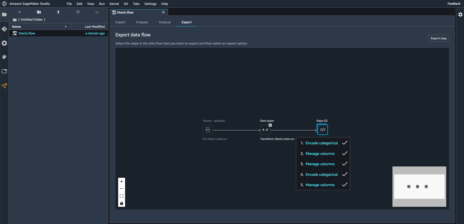
As you can see, SageMaker Clarify has some pretty powerful features for bias detection and explainability. Fortunately, it also makes them very easy to use. First, you should upload a clean and pre-processed copy of your tabular dataset (CSV or JSON) to Amazon Simple Storage Service (S3). Then, using a built-in container, you just launch an Amazon SageMaker Processing job on your dataset, passing a short configuration file defining the name of the target attribute, the name and values of the sensitive columns to analyze for bias, and the bias metrics that you want to compute. As you would expect, this job runs on fully managed infrastructure. For post-training analysis, a temporary endpoint is also automatically created and deleted by the job. Once the job is complete, results are available in S3 and in SageMaker Studio, and include an auto-generated report that summarizes the results.

Now, I’d like to show you how to get started with SageMaker Clarify.

Exploring Datasets and Models with Amazon SageMaker Clarify
The German Credit Data dataset contains 1,000 labeled credit applications, which I’ve used to train a binary classification model with XGBoost. Each data instance has 20 features, such as credit purpose, credit amount, housing status, employment history, and more. Categorical features have been encoded with Axx values. For example, here’s how the credit history feature is encoded: A30 means ‘no credits taken’, A31 means ‘all credits at this bank paid back duly’, and so on.

In particular, the dataset includes a feature telling us if a customer is a foreign worker. In fact, a quick look at the dataset hints at a large imbalance in favor of foreign workers. Could bias be hiding there? What about the model? Did XGBoost increase or decrease the bias? Which features contribute most to the predicted output? Let’s find out.

After training the model, my next step is to run a SageMaker Clarify bias analysis job on the dataset, using a built-in container image that will compute bias metrics. The job inputs are the dataset, and a JSON configuration file that defines:

  • The name of the target attribute (Class1Good2Bad), and the value for the positive answer (1).
  • The sensitive features to analyze (called “facets”), and their value. Here, we want to focus on instances where ForeignWorker is set to 0, as they seem to be under-represented in the dataset.
  • The bias metrics that the job should compute. As I already have a model, I pass its name so that post-training metrics can be computed on a temporary endpoint.

Here’s the relevant snippet in the configuration file:

"label": "Class1Good2Bad",
"label_values_or_threshold": [1],
"facet": [
        {
         "name_or_index" : "ForeignWorker",
         "value_or_threshold": [0]
        }
    ],
. . .
"methods": {
    "pre_training_bias": {"methods": "all"}
    "post_training_bias": {"methods": "all"}
},
"predictor": {
        "model_name": "xgboost-german-model",
        "instance_type": "ml.m5.xlarge",
        "initial_instance_count": 1
    }

Then, I configure the job inputs (the dataset and the configuration file) and output (the report), passing all appropriate paths in S3:

config_input = ProcessingInput(
                    input_name="analysis_config",
                    source=analysis_config_s3_path,
                    destination="/opt/ml/processing/input/config")
data_input = ProcessingInput(
                    input_name="dataset",
                    source=train_data_s3_path,
                    destination="/opt/ml/processing/input/data")
result_output = ProcessingOutput(
                    source="/opt/ml/processing/output",
                    destination=analysis_result_s3_path,
                    output_name="analysis_result")

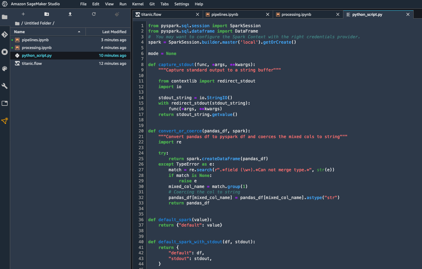
Finally, I run the processing job.

from sagemaker.processing import Processor, ProcessingInput, ProcessingJob, ProcessingOutput
analyzer_image_uri = f'678264136642.dkr.ecr.us-east-2.amazonaws.com/sagemaker-xai-analyzer:latest'
analyzer = Processor(base_job_name='analyzer',
                     image_uri=analyzer_image_uri,
                     role=sagemaker.get_execution_role(),
                     instance_count=1,
                     instance_type='ml.c5.xlarge')
analyzer.run(inputs=[ data_input, config_input], outputs=[result_output])

Once the processing job is complete, I can retrieve the report. Let’s look at bias metrics.

Detecting Bias with Amazon SageMaker Clarify
Here are some of the pre-training bias metrics:

"ForeignWorker": [
    {
     "value_or_threshold": "0",
     "metrics": [
      {
       "name": "CI",
       "description": "Class Imbalance (CI)",
       "value": 0.9225
      },
      {
       "name": "DPL",
       "description": "Difference in Positive Proportions in Labels (DPL)",
       "value": -0.21401904442300435
      },
. . . 

The class imbalance metric confirms our visual impression. The dataset has about 92% more foreign workers than it has domestic workers to assess. Whether this imbalance is responsible or not, we can also see that the difference in positive proportion for domestic workers is quite negative. In other words, there’s a smaller proportion of domestic workers with positive labels. This statistical pattern could be picked up by an ML algorithm, leading to a larger proportion of domestic workers getting negative answers. Figuring out whether this is actually legitimate or not would require further analysis, and in any case, it’s great that SageMaker Clarify warned us about this potential issue.

As I provided a trained model, post-training metrics are also available. Comparing the DPPL and the DPL, I can see that XGBoost has slightly reduced bias on positive proportions (-18.8% vs -21.4%). We also see that DAR is negative, indicating that the model achieves higher precision for domestic workers compared to foreign workers.

"ForeignWorker": [
    {
     "value_or_threshold": "0",
     "metrics": [
      {
       "name": "DPPL",
       "description": "\"Difference in Positive Proportions in Predicted Labels (DPPL)\")",
       "value": -0.18801124208230213
      },
      {
       "name": "DAR",
       "description": "Difference in Acceptance Rates (DAR)",
       "value": -0.050909090909090904
      },
      {
       "name": "DRR",
       "description": "Difference in Rejection Rates (DRR)",
       "value": 0.0365296803652968
      },
. . .

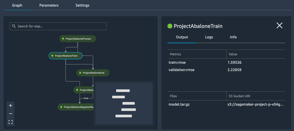
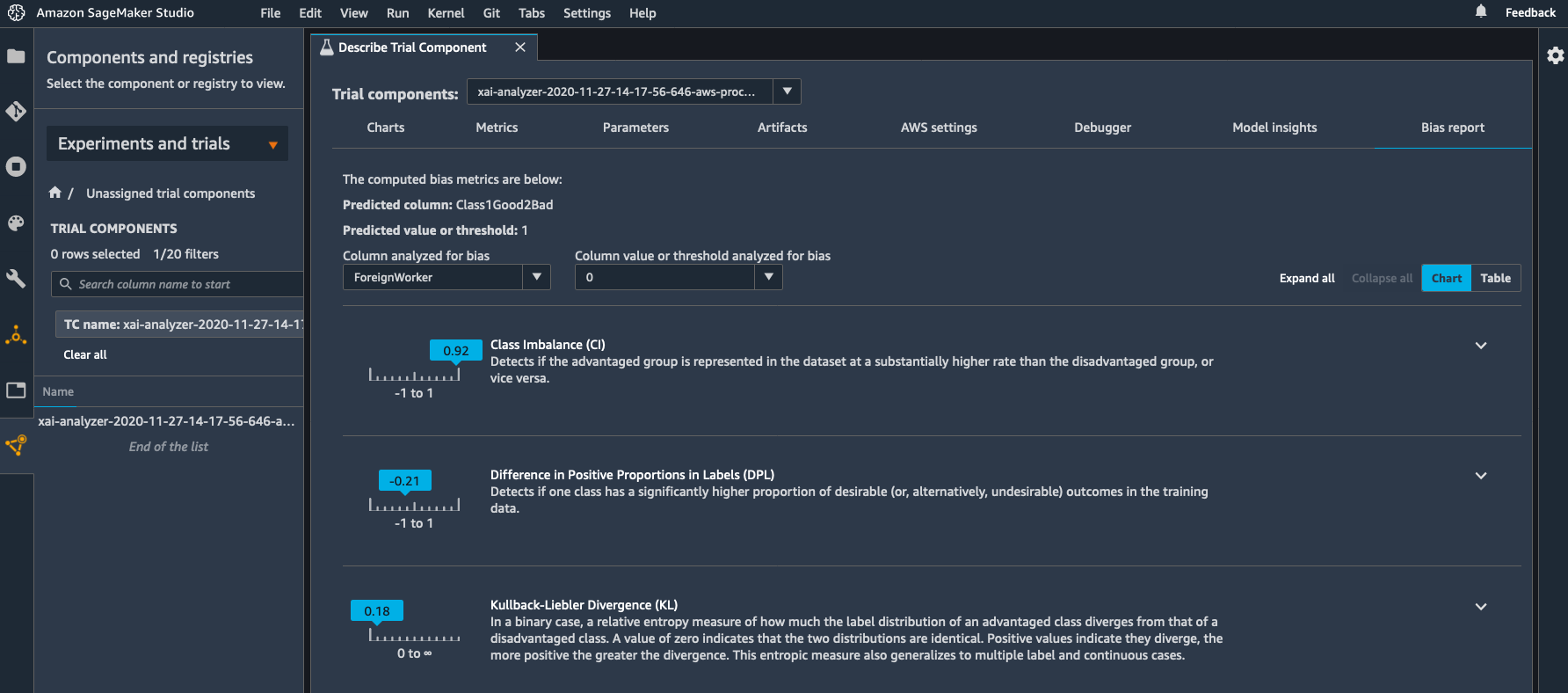
As SageMaker Clarify is integrated with SageMaker Studio, I can visualize bias metrics there. All I have to do is find the processing job in the list of trials, right-click “Open in trial details”, and select the “Bias report” view.

SageMaker screenshot

Finally, deciding whether high value of a certain bias metric is problematic involves domain-specific considerations. This needs to be guided by ethical, social, regulatory, and business considerations. Similarly, interventions for removing bias may often need a careful analysis of the entire ML lifecycle, from problem formulation to feedback loops in deployment.

Now, let’s see how SageMaker Clarify helps us understand what features the models base their predictions on.

Explaining Predictions with Amazon SageMaker Clarify
The report includes global SHAP values, showing the relative importance of all the features in the dataset. On the feature importance graph available in SageMaker Studio, I see that the three most important features are credit duration, not having a checking account (A14), and the loan amount. All things being equal, the bank probably sees you as a safer customer if you’re borrowing a small amount over a short period of time, and without the possibility to write checks!

SageMaker screenshot

In S3, I can also find a CSV file with SHAP values for individual data instances, giving me a complete picture of feature and feature value importance.

Getting Started
As you can see, SageMaker Clarify is a powerful tool to detect bias and to understand how your model works. You can start using it today in all regions where Amazon SageMaker is available, at no additional cost.

Sample notebooks are available to get you started quickly. Give them a try, and let us know what you think. We’re always looking forward to your feedback, either through your usual AWS support contacts, or on the AWS Forum for SageMaker.

– Julien

Special thanks to my colleagues Sanjiv Das, Michele Donini, Jason Gelman, Krishnaram Kenthapadi, Pinar Yilmaz, and Bilal Zafar for their precious help.

Dataset credits: Dua, D. and Graff, C. (2019). UCI Machine Learning Repository. Irvine, CA: University of California, School of Information and Computer Science.

New – Profile Your Machine Learning Training Jobs With Amazon SageMaker Debugger

Post Syndicated from Julien Simon original https://aws.amazon.com/blogs/aws/profile-your-machine-learning-training-jobs-with-amazon-sagemaker-debugger/

Today, I’m extremely happy to announce that Amazon SageMaker Debugger can now profile machine learning models, making it much easier to identify and fix training issues caused by hardware resource usage.

Despite its impressive performance on a wide range of business problems, machine learning (ML) remains a bit of a mysterious topic. Getting things right is an alchemy of science, craftsmanship (some would say wizardry), and sometimes luck. In particular, model training is a complex process whose outcome depends on the quality of your dataset, your algorithm, its parameters, and the infrastructure you’re training on.

As ML models become ever larger and more complex (I’m looking at you, deep learning), one growing issue is the amount of infrastructure required to train them. For instance, training BERT on the publicly available COCO dataset takes well over six hours on a single p3dn.24xlarge instance, even with its eight NVIDIA V100 GPUs. Some customers like autonomous vehicle companies deal with much larger datasets, and train object detection models for several days.

When a complex training job takes this long, the odds that something goes wrong and ruins it are pretty high, not only wasting time and money but also causing lots of frustration. Important work needs to be put on the back burner while you investigate, figure out the root cause, try to fix it, and then run your training job again. Often, you’ll have to iterate quite a few times to nail the problem.

Depending on the ML framework that you use, and sometimes on its version, you may or may not be able to use existing framework-specific tools. Often, you’ll have to build and maintain your own bespoke tools. Even for experienced practitioners, this is a lot of hard work. For regular developers like me, this is an utterly daunting task.

Introducing Model Profiling in Amazon SageMaker Debugger
Launched last year at AWS re:Invent, Amazon SageMaker Debugger is a capability of Amazon SageMaker that automatically identifies complex issues developing in ML training jobs. These include loss not decreasing, exploding gradients, and more.

Now, SageMaker Debugger can also monitor hardware resource usage, and allows you to profile your training job to help you correlate resource usage to ML operations in your training script. Thus, you’ll be able to resolve performance issues much quicker, and iterate through your training job much faster.

Chaim Rand, ML Algorithm Developer at Mobileye, an Intel company building automated driving and driver assistance systems, had the opportunity to work with the new profiling capabilities, and here’s what he told us: “Many of the assisted driving and autonomous vehicle technologies that we develop at Mobileye, rely on training deep neural network models to detect a wide variety of road artifacts, including vehicles, pedestrians, speed bumps, road signs and more. Often, these models train on extremely large datasets, on multiple machines, and for periods of up to several days. For us, at Mobileye, it is imperative that we have a toolkit of advanced performance profiling capabilities, for analyzing the flow of data across the network, CPU, and GPU resources, and for pinpointing performance issues. The profiling functionality in SageMaker Debugger provides just that, taking performance profiling out of the domain of a few specialized experts, and empowering our algorithm developers to maximize training resource utilization, accelerate model convergence, and reduce cost.

At launch, the new profiling capability of SageMaker Debugger is available for TensorFlow 2.x and PyTorch 1.x. All you have to do is to train with the corresponding built-in frameworks in Amazon SageMaker. Distributed training is supported out of the box.

Setting a single parameter in your SageMaker estimator, and without any change to your training code, you can enable the collection of infrastructure and model metrics such as:

  • CPU and GPU,
  • RAM and GPU RAM,
  • Network I/O,
  • Storage I/O (local storage and Pipe Mode),
  • Python metrics,
  • Data loading time,
  • Time spent in ML operators running on CPU and GPU,
  • Distributed training metrics for Horovod,
  • and many more.

In addition, you can visualize how much time is spent in different phases, such as preprocessing, training loop, and postprocessing. If needed, you can drill down on each training epoch, and even on each function in your training script.

By default, metrics are collected every 500ms, and you can also set this value to 100ms, 200ms, 1s, 5s, and 1min. For finer-grained analysis, you can also enable and disable profiling explicitly in your training code, only capturing metrics for specific parts.

While your training job is running, you can easily visualize these metrics in Amazon SageMaker Studio, our web-based integrated development environment for ML. As you would expect, all data is also available through the SageMaker Debugger API, and you can retrieve it to build your own graphs.

Running in parallel of the training job, an Amazon SageMaker Processing analyzes captured data, builds graphs, and generates a report providing insights on potential problems. This doesn’t require any work on your part, as this analysis runs inside a built-in container on fully managed infrastructure.

Now, let’s run a demo with PyTorch, where we’ll profile a ResNet-50 image classification model training on the CIFAR-10 dataset.

Profiling a Training Job with Amazon SageMaker Debugger
All it takes to enable profiling on your training job is an extra parameter in your SageMaker estimator. You don’t need to change a line in your training code. By default, SageMaker Debugger uses a set of built-in profiling rules looking for unwanted conditions that could develop during training, such as low GPU utilization. On top of reporting these conditions, SageMaker Debugger also triggers events in CloudWatch Events. For example, I could use them to run a AWS Lambda function that automatically stops inefficient training jobs.

First, I create a profiling configuration capturing data every 500ms. Optionally, I could select a training step interval if I wanted to profile only a certain portion of the job.

import sagemaker
from sagemaker.profiler import ProfilerConfig 
profiler_config = ProfilerConfig(profiling_interval_millis=500)

Then, I pass this configuration to my PyTorch Estimator, training on an ml.p3.8xlarge instance equipped with 4 NVIDIA V100 GPUs.

from sagemaker.pytorch import PyTorch
estimator = PyTorch(
    role=sagemaker.get_execution_role(),
    instance_count=1,
    instance_type='ml.p3.8xlarge',
    entry_point='train_pt.py',
    framework_version='1.5.0',
    hyperparameters={"batch_size":512, "epochs":10},
    profiler_config=profiler_config)

Then, I launch the training job as usual. Once the job is running, profiling data is captured and stored in S3.

path = estimator.latest_job_profiler_artifacts_path()
print(path)
s3://sagemaker-us-east-2-123456789012/pt-train-pt-2020-11-17-17-38-43-231/profiler-output

Using the SageMaker SDK, I can retrieve and count profiling events.

from smdebug.profiler.system_metrics_reader import S3SystemMetricsReader
system_metrics_reader = S3SystemMetricsReader(path)
system_metrics_reader.refresh_event_file_list()
last_timestamp = system_metrics_reader.get_timestamp_of_latest_available_file()
events = system_metrics_reader.get_events(0, last_timestamp)
print("Found", len(events), "recorded system metric events. Latest recorded event:", last_timestamp)
Found 411853 recorded system metric events. Latest recorded event: 1605620280000000

Of course, I could parse and analyze these profiling events, build my own graphs, and so on. Instead, let’s visualize them in near real-time in SageMaker Studio.

While my training job is still running, I locate it in SageMaker Studio, and I right-click “Open Debugger for insights”.

SageMaker screenshot

This opens a new tab, and I select the “Nodes” panel where I can see details statistics for each instance in my training job. So, how’s my training job doing? Feel free to click on the image below to zoom in.

SageMaker screenshot

Apparently, this job isn’t going great. GPU utilization and GPU memory utilization are desperately flat at around 10%. I’m definitely not pushing my multi-GPU instance hard enough. Maybe GPUs are not receiving data fast enough because the CPU can’t keep up? Let’s check the system utilization heatmap.

SageMaker screenshot

The CPU is taking a nap here, hardly ever exceeding 20% usage. This instance is definitely not busy enough. Is there anything I could do to fix this?

Switching to the “Overview” panel, I see that some of the built-in profiling rules have been triggered.

SageMaker screenshot

LowGPUUtilization confirms what I saw on the graphs above. BatchSize is very interesting, as it suggests increasing the size of mini-batches sent to the GPUs by the training script running on the CPU. This should definitely help fill GPU memory, put more GPU cores to work, speed up my training job, and improve infrastructure usage.

At this point, I should decide to stop my inefficient training job, and to relaunch it with a larger batch size. Here, I’ll let it run to completion to show you the report generated by the SageMaker Processing job running in parallel of your training job.

Once the training job is complete, I can see its summary in the “Overview” panel.

SageMaker screenshot

Clicking on the “Download report” button, I get a very detailed report that includes additional metrics, for example the ratio between the different phases of the training job, or the ratio between the forward and backward pass.

SageMaker screenshot

I can also see information on the most time-consuming CPU and GPU operators, which is really important if I wanted to optimize my code. For example, the graph below tells me that the most time-consuming GPU operations in my training job are backward pass convolution operators.

SageMaker screenshot

There’s much more to read in the report (rules summary, training loop analysis, and more). A companion notebook is also available to understand how graphs have been built, and how you can tailor them to your own needs.

Getting Started
We’ve just scratched the surface, and there are many more features in Amazon SageMaker Debugger that make it easy to gather, analyze and visualize model profiling information. You can start using it today in all regions where Amazon SageMaker is available. You won’t be charged for any compute used to run built-in profiling rules.

You’ll find sample notebooks on Github, so give them a try, and let us know what you think. We’re always looking forward to your feedback, either through your usual AWS support contacts, or on the AWS Forum for SageMaker.

– Julien

New – Managed Data Parallelism in Amazon SageMaker Simplifies Training on Large Datasets

Post Syndicated from Julien Simon original https://aws.amazon.com/blogs/aws/managed-data-parallelism-in-amazon-sagemaker-simplifies-training-on-large-datasets/

Today, I’m particularly happy to announce that Amazon SageMaker now supports a new data parallelism library that makes it easier to train models on datasets that may be as large as hundreds or thousands of gigabytes.

As data sets and models grow larger and more sophisticated, machine learning (ML) practitioners working on large distributed training jobs have to face increasingly long training times, even when using powerful instances such as the Amazon Elastic Compute Cloud (EC2) p3 and p4 instances. For example, using a ml.p3dn.24xlarge instance equipped with 8 NVIDIA V100 GPUs, it takes over 6 hours to train advanced object detection models such as Mask RCNN and Faster RCNN on the publicly available COCO dataset. Likewise, training BERT, a state of the art natural language processing model, takes over 100 hours on the same instance. Some of our customers, such as autonomous vehicle companies, routinely deal with even larger training jobs that run for days on large GPU clusters.

As you can imagine, these long training times are a severe bottleneck for ML projects, hurting productivity and slowing down innovation. Customers asked us for help, and we got to work.

Introducing Data Parallelism in Amazon SageMaker
Amazon SageMaker now helps ML teams reduce distributed training time and cost, thanks to the SageMaker Data Parallelism (SDP) library. Available for TensorFlow and PyTorch, SDP implements a more efficient distribution of computation, optimizes network communication, and fully utilizes our fastest p3 and p4 GPU instances.

Up to 90% of GPU resources can now be used for training, not for data transfer. Distributed training jobs can achieve up near-liner scaling efficiency, regardless of the number of GPUs involved. In other words, if a training job runs for 8 hours on a single instance, it will only take approximately 1 hour on 8 instances, with minimal cost increase. SageMaker effectively eliminates any trade-off between training cost and training time, allowing ML teams to get results sooner, iterate faster, and accelerate innovation.

During his keynote at AWS re:Invent 2020, Swami Sivasubramanian demonstrated the fastest training times to date for T5-3B and Mask-RCNN.

  • The T5-3B model has 3 billion parameters, achieves state-of-the-art accuracy on natural language processing benchmarks, and usually takes weeks of effort to train and tune for performance. We trained this model in 6 days on 256 ml.p4d.24xlarge instances.
  • Mask-RCNN continues to be a popular instance segmentation model used by our customers. Last year at re:Invent, we trained Mask-RCNN in 26 minutes on PyTorch, and in 27 minutes on TensorFlow. This year, we recorded the fastest training time to date for Mask-RCNN at 6:12 minutes on TensorFlow, and 6:45 minutes on PyTorch.

Before we explain how Amazon SageMaker is able to achieve such speedups, let’s first explain how data parallelism works, and why it’s hard to scale.

A Primer on Data Parallelism
If you’re training a model on a single GPU, its full internal state is available locally: model parameters, optimizer parameters, gradients (parameter updates computed by backpropagation), and so on. However, things are different when you distribute a training job to a cluster of GPUs.

Using a technique named “data parallelism,” the training set is split in mini-batches that are evenly distributed across GPUs. Thus, each GPU only trains the model on a fraction of the total data set. Obviously, this means that the model state will be slightly different on each GPU, as they will process different batches. In order to ensure training convergence, the model state needs to be regularly updated on all nodes. This can be done synchronously or asynchronously:

  • Synchronous training: all GPUs report their gradient updates either to all other GPUs (many-to-many communication), or to a central parameter server that redistributes them (many-to-one, followed by one-to-many). As all updates are applied simultaneously, the model state is in sync on all GPUs, and the next mini-batch can be processed.
  • Asynchronous training: gradient updates are sent to all other nodes, or to a central server. However, they are applied immediately, meaning that model state will differ from one GPU to the next.

Unfortunately, these techniques don’t scale very well. As the number of GPUs increases, a parameter server will inevitably become a bottleneck. Even without a parameter server, network congestion soon becomes a problem, as n GPUs need to exchange n*(n-1) messages after each iteration, for a total amount of n*(n-1)*model size bytes. For example, ResNet-50 is a popular model used in computer vision applications. With its 26 million parameters, each 32-bit gradient update takes about 100 megabytes. With 8 GPUs, each iteration requires sending and receiving 56 updates, for a total of 5.6 gigabytes. Even with a fast network, this will cause some overhead, and slow down training.

A significant step forward was taken in 2017 thanks to the Horovod project. Horovod implemented an optimized communication algorithm for distributed training named “ring-allreduce,” which was soon integrated with popular deep learning libraries.

In a nutshell, ring-allreduce is a decentralized asynchronous algorithm. There is no parameter server: nodes are organized in a directed cycle graph (to put it simply, a one-way ring). For each iteration, a node receives a gradient update from its predecessor. Once a node has processed its own batch, it applies both updates (its own and the one it received), and sends the results to its neighbor. With n GPUs, each GPU processes 2*(n-1) messages before all GPUs have been updated. Accordingly, the total amount of data exchanged per GPU is 2*(n-1)*model size, which is much better than n*(n-1)*model size.

Still, as datasets keep growing, the network bottleneck issue often rises again. Enter SageMaker and its new AllReduce algorithm.

A New Data Parallelism Algorithm in Amazon SageMaker
With the AllReduce algorithm, GPUs don’t talk to one another any more. Each GPU stores its gradient updates in GPU memory. When a certain threshold is exceeded, these updates are sharded, and sent to parameter servers running on the CPUs of the GPU instances. This removes the need for dedicated parameter servers.

Each CPU is responsible for a subset of the model parameters, and it receives updates coming from all GPUs. For example, with 3 training instances equipped with a single GPU, each GPU in the training cluster would send a third of its gradient updates to each one of the three CPUs.

Illustration

Then, each CPU would apply all the gradient updates that it received, and it would distributes the consolidated result back to all GPUs.

Illustration

Now that we understand how this algorithm works, let’s see how you can use it with your own code, without having to manage any infrastructure.

Training with Data Parallelism in Amazon SageMaker
The SageMaker Data Parallelism API is designed for ease of use, and should provide seamless integration with existing distributed training toolkits. In most cases, all you have to change in your training code is the import statement for Horovod (TensorFlow), or for Distributed Data Parallel (PyTorch).

For PyTorch, this would look like this.

import smdistributed.dataparallel.torch.parallel.distributed as dist
dist.init_process_group()

Then, I need to pin each GPU to a single SDP process.

torch.cuda.set_device(dist.get_local_rank())

Then, I define my model as usual, for example:

class Net(nn.Module):
    def __init__(self):
        super(Net, self).__init__()
        self.conv1 = nn.Conv2d(1, 32, 3, 1)
        self.conv2 = nn.Conv2d(32, 64, 3, 1)
        self.dropout1 = nn.Dropout2d(0.25)
        self.dropout2 = nn.Dropout2d(0.5)
        self.fc1 = nn.Linear(9216, 128)
        self.fc2 = nn.Linear(128, 10)
...

Finally, I instantiate my model, and use it to create a DistributedDataParallel object like so:

import torch
from smdistributed.dataparallel.torch.parallel.distributed import DistributedDataParallel as DDP
device = torch.device("cuda")
model = DDP(Net().to(device))

The rest of the code is vanilla PyTorch, and I can train it using the PyTorch estimator available in the SageMaker SDK. Here, I’m using an ml.p3.16xlarge instance with 8 NVIDIA V100 GPUs.

from sagemaker.pytorch import PyTorch
estimator = PyTorch(
    entry_point='train_pytorch.py',
    role=sagemaker.get_execution_role(),
    framework_version='1.6.0',
    instance_count=1,
    instance_type='ml.p3.16xlarge',
    distribution={'smdistributed':{'dataparallel':{enabled': True}}}
)
estimator.fit()

From then on, SageMaker takes over and provisions all required infrastructure. You can focus on other tasks while your training job runs.

Getting Started
If your training jobs last for hours or days on multiple GPUs, we believe that the SageMaker Data Parallelism library can save you time and money, and help you experiment and innovate quicker. It’s available today at in all regions where SageMaker is available, at no additional cost.

Examples are available to get you started quickly. Give them a try, and let us know what you think. We’re always looking forward to your feedback, either through your usual AWS support contacts, or on the AWS Forum for SageMaker.

– Julien

Amazon SageMaker Simplifies Training Deep Learning Models With Billions of Parameters

Post Syndicated from Julien Simon original https://aws.amazon.com/blogs/aws/amazon-sagemaker-simplifies-training-deep-learning-models-with-billions-of-parameters/

Today, I’m extremely happy to announce that Amazon SageMaker simplifies the training of very large deep learning models that were previously difficult to train due to hardware limitations.

In the last 10 years, a subset of machine learning named deep learning (DL) has taken the world by storm. Based on neural networks, DL algorithms have an extraordinary ability to extract information patterns hidden in vast amounts of unstructured data, such as images, videos, speech, or text. Indeed, DL has quickly achieved impressive results on a variety of complex human-like tasks, especially on computer vision and natural language processing. In fact, innovation has never been faster, as DL keeps improving its results on reference tasks like the ImageNet Large Scale Visual Recognition Challenge (ILSVRC), the General Language Understanding Evaluation (GLUE), or the Stanford Question Answering Dataset (SQUAD).

In order to tackle ever more complex tasks, DL researchers are designing increasingly sophisticated models, adding more neuron layers and more connections to improve pattern extraction and prediction accuracy, with a direct impact on model size. For example, you would get very good results on image classification with a 100-megabyte ResNet-50 model. For more difficult tasks such as object detection or instance segmentation, you would have to use larger models such as Mask R-CNN or YOLO v4, weighing in at about 250 megabytes.

As you can guess, model growth also impacts the amount of time and hardware resources required for model training, which is why Graphical Processing Units (GPU) have long been the preferred option to train and fine-tune large DL models. Thanks to their massively parallel architecture and their large on-board memory, they make it possible to use a technique called mini-batch training. By sending several data samples at once to the GPU, instead of sending them one by one, communication overhead is reduced, and training jobs are greatly accelerated. For example, the NVIDIA A100 available on the Amazon Elastic Compute Cloud (EC2) p4 family has over 7,000 compute cores and 40 gigabytes of fast onboard memory. Surely, that should be enough to train large batches of data on very large models, shouldn’t it?

Well, it’s not. Natural language processing behemoths such as OpenAI GPT-2 (1.5 billion parameters), T5-3B (3 billion parameters) and GPT-3 (175 billion parameters) consume tens or even hundreds of gigabytes of GPU memory. Likewise, state-of-the-art models working on high-resolution 3D images can be too large to fit in GPU memory, even with a batch size of 1…

Trying to square the circle, DL researchers use a combination of techniques, such as the following:

  • Buy more powerful GPUs, although we just saw that this is simply not an option for some models.
  • Work with less powerful models, and sacrifice accuracy.
  • Implement gradient checkpointing, a technique that relies on saving intermediate training results to disk instead of keeping everything in memory, at the expense of a 20-30% training slowdown.
  • Implement model parallelism, that is to say split the model manually, and train its (smaller) pieces on different GPUs. Needless to say, this is an extremely difficult, time-consuming, and uncertain task, even for expert practitioners.

Customers have told us that none of the above was a satisfactory solution to working with very large models. They asked us for a simpler and more cost-effective solution, and we got to work.

Introducing Model Parallelism in Amazon SageMaker
Model parallelism in SageMaker automatically and efficiently partitions models across several GPUs, eliminating the need for accuracy compromises or for complex manual work. In addition, thanks to this scale-out approach to model training, not only can you work with very large models without any memory bottleneck, you can also leverage a large number of smaller and more cost-effective GPUs.

At launch, this is supported for TensorFlow and PyTorch, and it only requires minimal changes in your code. When you launch a training job, you can specify whether your model should be optimized for speed or for memory usage. Then, Amazon SageMaker runs an initial profiling job on your behalf in order to analyze the compute and memory requirements of your model. This information is then fed to a partitioning algorithm which decides how to split the model and how to map model partitions to GPUs, while minimizing communication. The outcome of the partitioning decision is saved to a file, which is passed as input to the actual training job.

As you can see, SageMaker takes care of everything. If you’d like, you could also manually profile and partition the model, then train on SageMaker.

Before we look at the code, I’d like to give you a quick overview of the internals.

Training with Model Partitions and Microbatches
As model partitions running on different GPUs expect forward pass inputs from each other (activation values), processing training mini-batches across a sequence of partitions would only keep one partition busy at all times, while stalling the other ones.

To avoid this inefficient behavior, mini-batches are split into microbatches that are processed in parallel on the different GPUs. For example, GPU #1 could be forward propagating microbatch n, while GPU #2 could do the same for microbatch n+1. Activation values can be stored, and passed to the next partition whenever it’s ready to accept them.

For back propagation, partitions also expect input values from each other (gradients). As a partition can’t simultaneously run forward and backward propagation, we could wait for all GPUs to complete the forward pass on their own microbatch, before letting them run the corresponding backward pass. This simple mode is available in Amazon SageMaker.

There’s an even more efficient option, called interleaved mode. Here, SageMaker replicates partitions according to the number of microbatches. For example, working with 2 microbatches, each GPU would run two copies of the partition it has received. Each copy would collaborate with partitions running on other GPUs, either for forward or backpropagation.

Here’s how things could look like, with 4 different microbatches being processed by 2 duplicated partitions.

Illustration

To sum things up, interleaving the forward and backward passes of different microbatches is how SageMaker maximimes GPU utilization.

Now, let’s see how we can put this to work with TensorFlow.

Implementing Model Parallelism in Amazon SageMaker
Thanks to the SageMaker Model Parallelism (SMP) library, you can easily implement model parallelism in your own TensorFlow code (the process is similar for PyTorch). Here’s what you need to do:

  • Define and initialize the partitioning configuration.
  • Make your model a subclass of the DistributedModel class, using standard Keras subclassing.
  • Write and decorate with @smp.step a training function that represents a forward and backward step for the model. This function will be pipelined according to the architecture described in the previous section.
  • Optionally, do the same for an evaluation function that will also be pipelined.

Let’s apply this to a simple convolution network training on the MNIST dataset, using an ml.p3.8xlarge instance equipped with 4 NVIDIA V100 GPUs.

First, I initialize the SMP API.

import smdistributed.modelparallel.tensorflow as smp
smp.init()

Then, I subclass DistributedModel and build my model.

class MyModel(smp.DistributedModel):
    def __init__(self):
        super(MyModel, self).__init__()
        self.conv = Conv2D(32, 3, activation="relu")
        self.flatten = Flatten()
        self.dense1 = Dense(128)
        self.dense2 = Dense(10)
. . .

This is what the training function looks like.

@smp.step
def forward_backward(images, labels):
    predictions = model(images, training=True)
    loss = loss_obj(labels, predictions)
    grads = optimizer.get_gradients(loss, model.trainable_variables)
    return grads, loss

Then, I can train as usual with the TensorFlow estimator available in the SageMaker SDK. I only need to add the model parallelism configuration: 2 partitions (hence training on 2 GPUs), and 2 microbatches (hence 2 copies of each partition) with interleaving.

smd_mp_estimator = TensorFlow(
    entry_point="tf2.py",
    role=role,
    framework_version='2.3.1',
    pv_version='py3',
    instance_count=1,
    instance_type='ml.p3.16xlarge',
    distribution={
        "smdistributed": {
            "modelparallel": {
                "enabled":True,
                "parameters": {
                    "microbatches": 2,
                    "partitions": 2,
                    "pipeline": "interleaved",
                    "optimize": "memory",
                    "horovod": True, 
                }
             }
         },
        "mpi": {
            "enabled": True,
            "processes_per_host": 2, # Pick your processes_per_host
            "custom_mpi_options": mpioptions
        },
    }
)

Getting Started
As you can see, model parallelism makes it easier to train very large state-of-the-art deep learning models. It’s available today in all regions where Amazon SageMaker is available, at no additional cost.

Examples are available to get you started right away. Give them a try, and let us know what you think. We’re always looking forward to your feedback, either through your usual AWS support contacts, or on the AWS Forum for SageMaker.

– Julien


Amazon Monitron, a Simple and Cost-Effective Service Enabling Predictive Maintenance

Post Syndicated from Julien Simon original https://aws.amazon.com/blogs/aws/amazon-monitron-a-simple-cost-effective-service-enabling-predictive-maintenance/

Today, I’m extremely happy to announce Amazon Monitron, a condition monitoring service that detects potential failures and allows user to track developing faults enabling you to implement predictive maintenance and reduce unplanned downtime.

True story: A few months ago, I bought a new washing machine. As the delivery man was installing it in my basement, we were chatting about how unreliable these things seemed to be nowadays; never lasting more than a few years. As the gentleman made his way out, I pointed to my aging and poorly maintained water heater, telling him that I had decided to replace it in the coming weeks and that he’d be back soon to install a new one. Believe it or not, it broke down the next day. You can laugh at me, it’s OK. I deserve it for not planning ahead.

As annoying as this minor domestic episode was, it’s absolutely nothing compared to the tremendous loss of time and money caused by the unexpected failure of machines located in industrial environments, such as manufacturing production lines and warehouses. Any proverbial grain of sand can cause unplanned outages, and Murphy’s Law has taught us that they’re likely to happen in the worst possible configuration and at the worst possible time, resulting in severe business impacts.

To avoid breakdowns, reliability managers and maintenance technicians often combine three strategies:

  1. Run to failure: where equipment is operated without maintenance until it no longer operates reliably. When the repair is completed, equipment is returned to service; however, the condition of the equipment is unknown and failure is uncontrolled.
  2. Planned maintenance: where predefined maintenance activities are performed on a periodic or meter basis, regardless of condition. The effectiveness of planned maintenance activities is dependent on the quality of the maintenance instructions and planned cycle. It risks equipment being both over- and under-maintained, incurring unnecessary cost or still experiencing breakdowns.
  3. Condition-based maintenance: where maintenance is completed when the condition of a monitored component breaches a defined threshold. Monitoring physical characteristics such as tolerance, vibration or temperature is a more optimal strategy, requiring less maintenance and reducing maintenance costs.
  4. Predictive maintenance: where the condition of components is monitored, potential failures detected and developing faults tracked. Maintenance is planned at a time in the future prior to expected failure and when the total cost of maintenance is most cost-effective.

Condition-based maintenance and predictive maintenance require sensors to be installed on critical equipment. These sensors measure and capture physical quantities such as temperature and vibration, whose change is a leading indicator of a potential failure or a deteriorating condition.

As you can guess, building and deploying such maintenance systems can be a long, complex, and costly project involving bespoke hardware, software, infrastructure, and processes. Our customers asked us for help, and we got to work.

Introducing Amazon Monitron
Amazon Monitron is an easy and cost-effective condition monitoring service that allows you to monitor the condition of equipment in your facilities, enabling the implementation of a predictive maintenance program.

Illustration

Setting up Amazon Monitron is extremely simple. You first install Monitron sensors that capture vibration and temperature data from rotating machines, such as bearings, gearboxes, motors, pumps, compressors, and fans. Sensors send vibration and temperature measurements hourly to a nearby Monitron gateway, using Bluetooth Low Energy (BLE) technology allowing the sensors to run for at least three years. The Monitron gateway is itself connected to your WiFi network, and sends sensor data to AWS, where it is stored and analyzed using machine learning and ISO 20816 vibration standards.

As communication is infrequent, up to 20 sensors can be connected to a single gateway, which can be located up to 30 meters away (depending on potential interference). Thanks to the scalability and cost efficiency of Amazon Monitron, you can deploy as many sensors as you need, including on pieces of equipment that until now weren’t deemed critical enough to justify the cost of traditional sensors. As with any data-driven application, security is our No. 1 priority. The Monitron service authenticates the gateway and the sensors to make sure that they’re legitimate. Data is also encrypted end-to-end, without any decryption taking place on the gateway.

Setting up your gateways and sensors only requires installing the Monitron mobile application on an Android mobile device with Bluetooth support for gateway setup, and NFC support for sensor setup. This is an extremely simple process, and you’ll be monitoring in minutes. Technicians will also use the mobile application to receive alerts indicating abnormal machine conditions. They can acknowledge these alerts and provide feedback to improve their accuracy (say, to minimize false alerts and missed anomalies).

Customers are already using Amazon Monitron today, and here are a couple of examples.

Fender Musical Instruments Corporation is an iconic brand and a leading manufacturer of stringed instruments and amplifiers. Here’s what Bill Holmes, Global Director of Facilities at Fender, told us: “Over the past year we have partnered with AWS to help develop a critical but sometimes overlooked part of running a successful manufacturing business which is knowing the condition of your equipment. For manufacturers worldwide, uptime of equipment is the only way we can remain competitive with a global market. Ensuring equipment is up and running and not being surprised by sudden breakdowns helps get the most out of our equipment. Unplanned downtime is costly both in loss of production and labor due to the firefighting nature of the breakdown. The Amazon Monitron condition monitoring system has the potential of giving both large industry as well as small ‘mom and pop shops’ the ability to predict failures of their equipment before a catastrophic breakdown shuts them down. This will allow for a scheduled repair of failing equipment before it breaks down.

GE Gas Power is a leading provider of power generation equipment, solutions and services. It operates many manufacturing sites around the world, in which much of the manufacturing equipment is not connected nor monitored for health. Magnus Akesson, CIO at GE Gas Power Manufacturing says: “Naturally, we can reduce both maintenance costs and downtime, if we can easily and cheaply connect and monitor these assets at scale. Additionally, we want to take advantage of advanced algorithms to look forward, to know not just the current state but also predict future health and to detect abnormal behaviors. This will allow us to transition from time-based to predictive and prescriptive maintenance practices. Using Amazon Monitron, we are now able to quickly retrofit our assets with sensors and connecting them to real- time analytics in the AWS cloud. We can do this without having to require deep technical skills or having to configure our own IT and OT networks. From our initial work on vibration-prone tumblers, we are seeing this vision come to life at an amazing speed: the ease-of-use for the operators and maintenance team, the simplicity, and the ability to implement at scale is extremely attractive to GE. During our pilot, we were also delighted to see one-click capabilities for updating the sensors via remote Over the Air (OTA) firmware upgrades, without having to physically touch the sensors. As we grow in scale, this is a critical capability in order to be able to support and maintain the fleet of sensors.

Now, let me show you how to get started with Amazon Monitron.

Setting up Amazon Monitron
First, I open the Monitron console. In just a few clicks, I create a project, and an administrative user allowed to manage it. Using a link provided in the console, I download and install the Monitron mobile application on my Android phone. Opening the app, I log in using my administrative credentials.

The first step is to create a site describing assets, sensors, and gateways. I name it “my-thor-project.”

Application screenshot

Let’s add a gateway. Enabling BlueTooth on my phone, I press the pairing button on the gateway.

Application screenshot

The name of the gateway appears immediately.

Application screenshot

I select the gateway, and I configure it with my WiFi credentials to let it connect to AWS. A few seconds later, the gateway is online.

Application screenshot

My next step is to create an asset that I’d like to monitor, say a process water pump set, with a motor and a pump that I would like to monitor. I first create the asset itself, simply defining its name, and the appropriate ISO 20816 class (a standard for measurement and evaluation of machine vibration).

Application screenshot

Then, I add a sensor for the motor.

Application screenshot

I start by physically attaching the sensor to the motor using the suggested adhesive. Next, I specify a sensor position, enable the NFC on my smartphone, and tap the Monitron sensor that I attached to the motor with my phone. Within seconds, the sensor is commissioned.

Application screenshot

I repeat the same operation for the pump. Looking at my asset, I see that both sensors are operational.

Application screenshot

They are now capturing temperature and vibration information. Although there isn’t much to see for the moment, graphs are available in the mobile app.

Application screenshot

Over time, the gateway will keep sending this data securely to AWS, where it will be analyzed for early signs of failure. Should either of my assets exhibit these, I would receive an alert in the mobile application, where I could visualize historical data, and decide what the best course of action would be.

Getting Started
As you can see, Monitron makes it easy to deploy sensors enabling predictive maintenance applications. The service is available today in the US East (N. Virginia) region, and using it costs $50 per sensor per year.

If you’d like to evaluate the service, the Monitron Starter Kit includes everything you need (a gateway with a mounting kit, five sensors, and a power supply), and it’s available for $715. Then, you can scale your deployment with additional sensors, which you can buy in 5-packs for $575.

Starter kit picture

Give Amazon Monitron a try, and let us know what you think. We’re always looking forward to your feedback, either through your usual AWS support contacts, or on the AWS Forum for Monitron.

– Julien

Special thanks to my colleague Dave Manley for taking the time to educate me on industrial maintenance operations.

Amazon SageMaker Continues to Lead the Way in Machine Learning and Announces up to 18% Lower Prices on GPU Instances

Post Syndicated from Julien Simon original https://aws.amazon.com/blogs/aws/amazon-sagemaker-leads-way-in-machine-learning/

Since 2006, Amazon Web Services (AWS) has been helping millions of customers build and manage their IT workloads. From startups to large enterprises to public sector, organizations of all sizes use our cloud computing services to reach unprecedented levels of security, resiliency, and scalability. Every day, they’re able to experiment, innovate, and deploy to production in less time and at lower cost than ever before. Thus, business opportunities can be explored, seized, and turned into industrial-grade products and services.

As Machine Learning (ML) became a growing priority for our customers, they asked us to build an ML service infused with the same agility and robustness. The result was Amazon SageMaker, a fully managed service launched at AWS re:Invent 2017 that provides every developer and data scientist with the ability to build, train, and deploy ML models quickly.

Today, Amazon SageMaker is helping tens of thousands of customers in all industry segments build, train and deploy high quality models in production: financial services (Euler Hermes, Intuit, Slice Labs, Nerdwallet, Root Insurance, Coinbase, NuData Security, Siemens Financial Services), healthcare (GE Healthcare, Cerner, Roche, Celgene, Zocdoc), news and media (Dow Jones, Thomson Reuters, ProQuest, SmartNews, Frame.io, Sportograf), sports (Formula 1, Bundesliga, Olympique de Marseille, NFL, Guiness Six Nations Rugby), retail (Zalando, Zappos, Fabulyst), automotive (Atlas Van Lines, Edmunds, Regit), dating (Tinder), hospitality (Hotels.com, iFood), industry and manufacturing (Veolia, Formosa Plastics), gaming (Voodoo), customer relationship management (Zendesk, Freshworks), energy (Kinect Energy Group, Advanced Microgrid Systems), real estate (Realtor.com), satellite imagery (Digital Globe), human resources (ADP), and many more.

When we asked our customers why they decided to standardize their ML workloads on Amazon SageMaker, the most common answer was: “SageMaker removes the undifferentiated heavy lifting from each step of the ML process.” Zooming in, we identified five areas where SageMaker helps them most.

#1 – Build Secure and Reliable ML Models, Faster
As many ML models are used to serve real-time predictions to business applications and end users, making sure that they stay available and fast is of paramount importance. This is why Amazon SageMaker endpoints have built-in support for load balancing across multiple AWS Availability Zones, as well as built-in Auto Scaling to dynamically adjust the number of provisioned instances according to incoming traffic.

For even more robustness and scalability, Amazon SageMaker relies on production-grade open source model servers such as TensorFlow Serving, the Multi-Model Server, and TorchServe. A collaboration between AWS and Facebook, TorchServe is available as part of the PyTorch project, and makes it easy to deploy trained models at scale without having to write custom code.

In addition to resilient infrastructure and scalable model serving, you can also rely on Amazon SageMaker Model Monitor to catch prediction quality issues that could happen on your endpoints. By saving incoming requests as well as outgoing predictions, and by comparing them to a baseline built from a training set, you can quickly identify and fix problems like missing features or data drift.

Says Aude Giard, Chief Digital Officer at Veolia Water Technologies: “In 8 short weeks, we worked with AWS to develop a prototype that anticipates when to clean or change water filtering membranes in our desalination plants. Using Amazon SageMaker, we built a ML model that learns from previous patterns and predicts the future evolution of fouling indicators. By standardizing our ML workloads on AWS, we were able to reduce costs and prevent downtime while improving the quality of the water produced. These results couldn’t have been realized without the technical experience, trust, and dedication of both teams to achieve one goal: an uninterrupted clean and safe water supply.” You can learn more in this video.

#2 – Build ML Models Your Way
When it comes to building models, Amazon SageMaker gives you plenty of options. You can visit AWS Marketplace, pick an algorithm or a model shared by one of our partners, and deploy it on SageMaker in just a few clicks. Alternatively, you can train a model using one of the built-in algorithms, or your own code written for a popular open source ML framework (TensorFlow, PyTorch, and Apache MXNet), or your own custom code packaged in a Docker container.

You could also rely on Amazon SageMaker AutoPilot, a game-changing AutoML capability. Whether you have little or no ML experience, or you’re a seasoned practitioner who needs to explore hundreds of datasets, SageMaker AutoPilot takes care of everything for you with a single API call. It automatically analyzes your dataset, figures out the type of problem you’re trying to solve, builds several data processing and training pipelines, trains them, and optimizes them for maximum accuracy. In addition, the data processing and training source code is available in auto-generated notebooks that you can review, and run yourself for further experimentation. SageMaker Autopilot also now creates machine learning models up to 40% faster with up to 200% higher accuracy, even with small and imbalanced datasets.

Another popular feature is Automatic Model Tuning. No more manual exploration, no more costly grid search jobs that run for days: using ML optimization, SageMaker quickly converges to high-performance models, saving you time and money, and letting you deploy the best model to production quicker.

NerdWallet relies on data science and ML to connect customers with personalized financial products“, says Ryan Kirkman, Senior Engineering Manager. “We chose to standardize our ML workloads on AWS because it allowed us to quickly modernize our data science engineering practices, removing roadblocks and speeding time-to-delivery. With Amazon SageMaker, our data scientists can spend more time on strategic pursuits and focus more energy where our competitive advantage is—our insights into the problems we’re solving for our users.” You can learn more in this case study.
Says Tejas Bhandarkar, Senior Director of Product, Freshworks Platform: “We chose to standardize our ML workloads on AWS because we could easily build, train, and deploy machine learning models optimized for our customers’ use cases. Thanks to Amazon SageMaker, we have built more than 30,000 models for 11,000 customers while reducing training time for these models from 24 hours to under 33 minutes. With SageMaker Model Monitor, we can keep track of data drifts and retrain models to ensure accuracy. Powered by Amazon SageMaker, Freddy AI Skills is constantly-evolving with smart actions, deep-data insights, and intent-driven conversations.

#3 – Reduce Costs
Building and managing your own ML infrastructure can be costly, and Amazon SageMaker is a great alternative. In fact, we found out that the total cost of ownership (TCO) of Amazon SageMaker over a 3-year horizon is over 54% lower compared to other options, and developers can be up to 10 times more productive. This comes from the fact that Amazon SageMaker manages all the training and prediction infrastructure that ML typically requires, allowing teams to focus exclusively on studying and solving the ML problem at hand.

Furthermore, Amazon SageMaker includes many features that help training jobs run as fast and as cost-effectively as possible: optimized versions of the most popular machine learning libraries, a wide range of CPU and GPU instances with up to 100GB networking, and of course Managed Spot Training which lets you save up to 90% on your training jobs. Last but not least, Amazon SageMaker Debugger automatically identifies complex issues developing in ML training jobs. Unproductive jobs are terminated early, and you can use model information captured during training to pinpoint the root cause.

Amazon SageMaker also helps you slash your prediction costs. Thanks to Multi-Model Endpoints, you can deploy several models on a single prediction endpoint, avoiding the extra work and cost associated with running many low-traffic endpoints. For models that require some hardware acceleration without the need for a full-fledged GPU, Amazon Elastic Inference lets you save up to 90% on your prediction costs. At the other end of the spectrum, large-scale prediction workloads can rely on AWS Inferentia, a custom chip designed by AWS, for up to 30% higher throughput and up to 45% lower cost per inference compared to GPU instances.

Lyft, one of the largest transportation networks in the United States and Canada, launched its Level 5 autonomous vehicle division in 2017 to develop a self-driving system to help millions of riders. Lyft Level 5 aggregates over 10 terabytes of data each day to train ML models for their fleet of autonomous vehicles. Managing ML workloads on their own was becoming time-consuming and expensive. Says Alex Bain, Lead for ML Systems at Lyft Level 5: “Using Amazon SageMaker distributed training, we reduced our model training time from days to couple of hours. By running our ML workloads on AWS, we streamlined our development cycles and reduced costs, ultimately accelerating our mission to deliver self-driving capabilities to our customers.

#4 – Build Secure and Compliant ML Systems
Security is always priority #1 at AWS. It’s particularly important to customers operating in regulated industries such as financial services or healthcare, as they must implement their solutions with the highest level of security and compliance. For this purpose, Amazon SageMaker implements many security features, making it compliant with the following global standards: SOC 1/2/3, PCI, ISO, FedRAMP, DoD CC SRG, IRAP, MTCS, C5, K-ISMS, ENS High, OSPAR, and HITRUST CSF. It’s also HIPAA BAA eligible.

Says Ashok Srivastava, Chief Data Officer, Intuit: “With Amazon SageMaker, we can accelerate our Artificial Intelligence initiatives at scale by building and deploying our algorithms on the platform. We will create novel large-scale machine learning and AI algorithms and deploy them on this platform to solve complex problems that can power prosperity for our customers.”

#5 – Annotate Data and Keep Humans in the Loop
As ML practitioners know, turning data into a dataset requires a lot of time and effort. To help you reduce both, Amazon SageMaker Ground Truth is a fully managed data labeling service that makes it easy to annotate and build highly accurate training datasets at any scale (text, image, video, and 3D point cloud datasets).

Says Magnus Soderberg, Director, Pathology Research, AstraZeneca: “AstraZeneca has been experimenting with machine learning across all stages of research and development, and most recently in pathology to speed up the review of tissue samples. The machine learning models first learn from a large, representative data set. Labeling the data is another time-consuming step, especially in this case, where it can take many thousands of tissue sample images to train an accurate model. AstraZeneca uses Amazon SageMaker Ground Truth, a machine learning-powered, human-in-the-loop data labeling and annotation service to automate some of the most tedious portions of this work, resulting in reduction of time spent cataloging samples by at least 50%.

Amazon SageMaker is Evaluated
The hundreds of new features added to Amazon SageMaker since launch are testimony to our relentless innovation on behalf of customers. In fact, the service was highlighted in February 2020 as the overall leader in Gartner’s Cloud AI Developer Services Magic Quadrant. Gartner subscribers can click here to learn more about why we have an overall score of 84/100 in their “Solution Scorecard for Amazon SageMaker, July 2020”, the highest rating among our peer group. According to Gartner, we met 87% of required criteria, 73% of preferred, and 85% of optional.

Announcing a Price Reduction on GPU Instances

To thank our customers for their trust and to show our continued commitment to make Amazon SageMaker the best and most cost-effective ML service, I’m extremely happy to announce a significant price reduction on all ml.p2 and ml.p3 GPU instances. It will apply starting October 1st for all SageMaker components and across the following regions: US East (N. Virginia), US East (Ohio), US West (Oregon), EU (Ireland), EU (Frankfurt), EU (London), Canada (Central), Asia Pacific (Singapore), Asia Pacific (Sydney), Asia Pacific (Seoul), Asia Pacific (Tokyo), Asia Pacific (Mumbai), and AWS GovCloud (US-Gov-West).

Instance Name Price Reduction
ml.p2.xlarge -11%
ml.p2.8xlarge -14%
ml.p2.16xlarge -18%
ml.p3.2xlarge -11%
ml.p3.8xlarge -14%
ml.p3.16xlarge -18%
ml.p3dn.24xlarge -18%

Getting Started with Amazon SageMaker
As you can see, there are a lot of exciting features in Amazon SageMaker, and I encourage you to try them out! Amazon SageMaker is available worldwide, so chances are you can easily get to work on your own datasets. The service is part of the AWS Free Tier, letting new users work with it for free for hundreds of hours during the first two months.

If you’d like to kick the tires, this tutorial will get you started in minutes. You’ll learn how to use SageMaker Studio to build, train, and deploy a classification model based on the XGBoost algorithm.

Last but not least, I just published a book named “Learn Amazon SageMaker“, a 500-page detailed tour of all SageMaker features, illustrated by more than 60 original Jupyter notebooks. It should help you get up to speed in no time.

As always, we’re looking forward to your feedback. Please share it with your usual AWS support contacts, or on the AWS Forum for SageMaker.

– Julien

Amazon Transcribe Now Supports Automatic Language Identification

Post Syndicated from Julien Simon original https://aws.amazon.com/blogs/aws/amazon-transcribe-now-supports-automatic-language-identification/

In 2017, we launched Amazon Transcribe, an automatic speech recognition service that makes it easy for developers to add a speech-to-text capability to their applications. Since then, we added support for more languages, enabling customers globally to transcribe audio recordings in 31 languages, including 6 in real-time.

A popular use case for Amazon Transcribe is transcribing customer calls. This allows companies to analyze the transcribed text using natural language processing techniques to detect sentiment or to identify the most common call causes. If you operate in a country with multiple official languages or across multiple regions, your audio files can contain different languages. Thus, files have to be tagged manually with the appropriate language before transcription can take place. This typically involves setting up teams of multi-lingual speakers, which creates additional costs and delays in processing audio files.

The media and entertainment industry often uses Amazon Transcribe to convert media content into accessible and searchable text files. Use cases include generating subtitles or transcripts, moderating content, and more. Amazon Transcribe is also used by operations team for quality control, for example checking that audio and video are in sync thanks to the timestamps present in the extracted text. However, other problems couldn’t be easily solved, such as verifying that the main spoken language in your videos is correctly labeled to avoid streaming video in the wrong language.

Today, I’m extremely happy to announce that Amazon Transcribe can now automatically identify the dominant language in an audio recording. This feature will help customers build more efficient transcription workflows by getting rid of manual tagging. In addition to the examples mentioned above, you can now also easily use Amazon Transcribe to automatically recognize and transcribe voicemails, meetings, and any form of recorded communication.

Introducing Automatic Language Identification
With a minimum of 30 seconds of audio, Amazon Transcribe can efficiently generate transcripts in the spoken language without wasting time and resources on manual tagging. Automatic identification of the dominant language is available in batch transcription mode for all 31 languages. Thanks to sampling techniques, language identification happens much faster than the transcription itself, in the matter of seconds.

If you’re already using Amazon Transcribe for speech recognition, you just need to enable the feature in the StartTranscriptionJob API. Before your transcription job is complete, the response of the GetTranscriptionJob API will tell the dominant language of the audio recording, and its confidence score between 0 and 1. The transcript lists the top five languages and their respective confidence scores.

Of course, if you want to use Amazon Transcribe exclusively for automatic language identification, you can simply process the API response and ignore the transcript. In this case, you should stick to short 30-45 second audio recordings to minimize costs.

You can also restrict languages that Amazon Transcribe tries to identify, by passing a list of languages to the StartTranscriptionJob API. For example, if your company call center only receives calls in English, Spanish and French, then restricting identifiable languages to this list will increase language identification accuracy.

Now, I’d like to show you how easy it us to use this new feature!

Detecting the Dominant Language With Amazon Transcribe
First, let’s try a high quality sample. I’ll use the audio track from one of my breakout sessions at AWS Summit Paris 2019. I can easily download it using the youtube-dl tool.

$ youtube-dl -f bestaudio https://www.youtube.com/watch?v=AFN5jaTurfA
$ mv AWS\ \&\ EarthCube\ _\ Deep\ learning\ démarrer\ avec\ MXNet\ et\ Tensorflow\ en\ 10\ minutes-AFN5jaTurfA.m4a video.m4a

Using ffmpeg, I shorten the audio clip to 1 minute.

$ ffmpeg -i video.m4a -ss 00:00:00.00 -t 00:01:00.00 video-1mn.m4a

Then, I upload the clip to an Amazon Simple Storage Service (S3) bucket.

$ aws s3 cp video-1mn.m4a s3://jsimon-transcribe-uswest2/

Next, I use the AWS CLI to run a transcription job on this audio clip, with language identification enabled.

$ awscli transcribe start-transcription-job --transcription-job-name video-test --identify-language --media MediaFileUri=s3://jsimon-transcribe-uswest2/video-1mn.m4a

Waiting only a few seconds, I check the status of the job. I could also use a Amazon CloudWatch event to be notified that language identification is complete.

$ awscli transcribe get-transcription-job --transcription-job-name video-test
{
    "TranscriptionJob": {
        "TranscriptionJobName": "video-test",
        "TranscriptionJobStatus": "IN_PROGRESS",
        "LanguageCode": "fr-FR",
        "MediaSampleRateHertz": 44100,
        "MediaFormat": "mp4",
        "Media": {
        "MediaFileUri": "s3://jsimon-transcribe-uswest2/video-1mn.m4a"
    },
    "Transcript": {},
    "StartTime": 1593704323.312,
"CreationTime": 1593704323.287,

    "Settings": {
        "ChannelIdentification": false,
        "ShowAlternatives": false
    },
    "IdentifyLanguage": true,
    "IdentifiedLanguageScore": 0.915885329246521
    }
}

As highlighted in the output, the dominant language has been correctly detected in seconds, with a high confidence score of 91.59%. A few more seconds later, the transcription job is complete. Running the same CLI call, I can retrieve a link to the transcription, which also includes the top 5 languages for the audio clip, sorted by decreasing score.

"language_identification":[{"score":"0.9159","code":"fr-FR"},{"score":"0.0839","code":"fr-CA"},{"score":"0.0001","code":"en-GB"},{"score":"0.0001","code":"pt-PT"},{"score":"0.0001","code":"de-CH"}]

Adding up French and Canadian French, we pretty much get a score of 100%, so there’s no doubt that this clip is in French. In some cases, you may not care for that level of detail, and you’ll see in the next example how to restrict the list of detected languages.

Restricting the List of Detected Languages
As customer call transcription is a popular use case for Amazon Transcribe, here is a 40-second audio clip (WAV, 8KHz, 16-bit resolution), where I’m reading a paragraph from the French version of the Amazon Transcribe page. As you can hear, quality is pretty awful, and I added background music (Bach-ground, actually) for good measure.

Again, I upload the clip to an S3 bucket, and I use the AWS CLI to transcribe it. This time, I restrict the list of languages to French, Spanish, German, US English, and British English.

$ aws s3 cp speech-8k.wav s3://jsimon-transcribe-uswest2/
$ awscli transcribe start-transcription-job --transcription-job-name speech-8k-test --identify-language --media MediaFileUri=s3://jsimon-transcribe-uswest2/speech-8k.wav --language-options fr-FR es-ES de-DE en-US en-GB

A few seconds later, I check the status of the job.

$ awscli transcribe get-transcription-job --transcription-job-name speech-8k-test
{
    "TranscriptionJob": {
    "TranscriptionJobName": "speech-8k-test",
    "TranscriptionJobStatus": "IN_PROGRESS",
    "LanguageCode": "fr-FR",
    "MediaSampleRateHertz": 8000,
    "MediaFormat": "wav",
    "Media": {
        "MediaFileUri": "s3://jsimon-transcribe-uswest2/speech-8k.wav"
    },
    "Transcript": {},
    "StartTime": 1593705151.446,
"CreationTime": 1593705151.423,

    "Settings": {
        "ChannelIdentification": false,
        "ShowAlternatives": false
    },
    "IdentifyLanguage": true,
    "LanguageOptions": [
        "fr-FR","es-ES","de-DE","en-US","en-GB"
    ],
    "IdentifiedLanguageScore": 0.9995
    }
}

As highlighted in the output, the dominant language has been correctly detected with a very high confidence score in spite of the terrible audio quality. Restricting the list of languages certainly helps, and you should use it whenever possible.

Getting Started
Automatic Language Identification is available today in these regions:

  • US East (N. Virginia), US East (Ohio), US West (N. California), US West (Oregon), AWS GovCloud (US-West).
  • Canada (Central).
  • South America (São Paulo).
  • Europe (Ireland), Europe (London), Europe (Paris), Europe (Frankfurt).
  • Middle East (Bahrain).
  • Asia Pacific (Hong Kong), Asia Pacific (Mumbai), Asia Pacific (Tokyo), Asia Pacific (Seoul), Asia Pacific (Singapore), Asia Pacific (Sydney).

There is no additional charge on top of the existing pricing. Give it a try, and please send us feedback either through your usual AWS Support contacts, or on the AWS Forum for Amazon Transcribe.

– Julien