Post Syndicated from Danilo Poccia original https://aws.amazon.com/blogs/aws/introducing-amazon-bedrock-agentcore-securely-deploy-and-operate-ai-agents-at-any-scale/
In just a few years, foundation models (FMs) have evolved from being used directly to create content in response to a user’s prompt, to now powering AI agents, a new class of software applications that use FMs to reason, plan, act, learn, and adapt in pursuit of user-defined goals with limited human oversight. This new wave of agentic AI is enabled by the emergence of standardized protocols such as Model Context Protocol (MCP) and Agent2Agent (A2A) that simplify how agents connect with other tools and systems.
In fact, building AI agents that can reliably perform complex tasks has become increasingly accessible thanks to open source frameworks like CrewAI, LangGraph, and Strands Agents. However, moving from a promising proof-of-concept to a production-ready agent that can scale to thousands of users presents significant challenges.
Instead of being able to focus on the core features of the agent, developers and AI engineers have to spend months building foundational infrastructure for session management, identity controls, memory systems, and observability—at the same time supporting security and compliance.
Today, we’re excited to announce the preview of Amazon Bedrock AgentCore, a comprehensive set of enterprise-grade services that help developers quickly and securely deploy and operate AI agents at scale using any framework and model, hosted on Amazon Bedrock or elsewhere.
More specifically, we are introducing today:
AgentCore Runtime – Provides sandboxed low-latency serverless environments with session isolation, supporting any agent framework including popular open source frameworks, tools, and models, and handling multimodal workloads and long-running agents.
AgentCore Memory – Manages session and long-term memory, providing relevant context to models while helping agents learn from past interactions.
AgentCore Observability – Offers step-by-step visualization of agent execution with metadata tagging, custom scoring, trajectory inspection, and troubleshooting/debugging filters.
AgentCore Identity – Enables AI agents to securely access AWS services and third-party tools and services such as GitHub, Salesforce, and Slack, either on behalf of users or by themselves with pre-authorized user consent.
AgentCore Gateway – Transforms existing APIs and AWS Lambda functions into agent-ready tools, offering unified access across protocols, including MCP, and runtime discovery.
AgentCore Browser – Provides managed web browser instances to scale your agents’ web automation workflows.
AgentCore Code Interpreter – Offers an isolated environment to run the code your agents generate.
These services can be used individually and are optimized to work together so developers don’t need to spend time piecing together components. AgentCore can work with open source or custom AI agent frameworks, giving teams the flexibility to maintain their preferred tools while gaining enterprise capabilities. To integrate these services into their existing code, developers can use the AgentCore SDK.
You can now discover, buy, and run pre-built agents and agent tools from AWS Marketplace with AgentCore Runtime. With just a few lines of code, your agents can securely connect to API-based agents and tools from AWS Marketplace with AgentCore Gateway to help you run complex workflows while maintaining compliance and control.
AgentCore eliminates tedious infrastructure work and operational complexity so development teams can bring groundbreaking agentic solutions to market faster.
Let’s see how this works in practice. I’ll share more info on the services as we use them.
Deploying a production-ready customer support assistant with Amazon Bedrock AgentCore (Preview)
When customers reach out with an email, it takes time to provide a reply. Customer support needs to check the validity of the email, find who the actual customer is in the customer relationship management (CRM) system, check their orders, and use product-specific knowledge bases to find the information required to prepare an answer.
An AI agent can simplify that by connecting to the internal systems, retrieve contextual information using a semantic data source, and draft a reply for the support team. For this use case, I built a simple prototype using Strands Agents. For simplicity and to validate the scenario, the internal tools are simulated using Python functions.
When I talk to developers, they tell me that similar prototypes, covering different use cases, are being built in many companies. When these prototypes are demonstrated to the company leadership and receive confirmation to proceed, the development team has to define how to go in production and satisfy the usual requirements for security, performance, availability, and scalability. This is where AgentCore can help.
Step 1 – Deploying to the cloud with AgentCore Runtime
AgentCore Runtime is a new service to securely deploy, run, and scale AI agents, providing isolation so that each user session runs in its own protected environment to help prevent data leakage—a critical requirement for applications handling sensitive data.
To match different security postures, agents can use different network configurations:
Sandbox – To only communicate with allowlisted AWS services.
Public – To run with managed internet access.
VPC-only (coming soon) – This option will allow to access resources hosted in a customer’s VPC or connected via AWS PrivateLink endpoints.
To deploy the agent to the cloud and get a secure, serverless endpoint with AgentCore Runtime, I add to the prototype a few lines of code using the AgentCore SDK to:
- Import the AgentCore SDK.
- Create the AgentCore app.
- Specify which function is the entry point to invoke the agent.
Using a different or custom agent framework is a matter of replacing the agent invocation inside the entry point function.
Here’s the code of the prototype. The three lines I added to use AgentCore Runtime are the ones preceded by a comment.
from strands import Agent, tool
from strands_tools import calculator, current_time
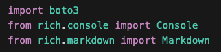
# Import the AgentCore SDK
from bedrock_agentcore.runtime import BedrockAgentCoreApp
WELCOME_MESSAGE = """
Welcome to the Customer Support Assistant! How can I help you today?
"""
SYSTEM_PROMPT = """
You are an helpful customer support assistant.
When provided with a customer email, gather all necessary info and prepare the response email.
When asked about an order, look for it and tell the full description and date of the order to the customer.
Don't mention the customer ID in your reply.
"""
@tool
def get_customer_id(email_address: str):
if email_address == "[email protected]":
return { "customer_id": 123 }
else:
return { "message": "customer not found" }
@tool
def get_orders(customer_id: int):
if customer_id == 123:
return [{
"order_id": 1234,
"items": [ "smartphone", "smartphone USB-C charger", "smartphone black cover"],
"date": "20250607"
}]
else:
return { "message": "no order found" }
@tool
def get_knowledge_base_info(topic: str):
kb_info = []
if "smartphone" in topic:
if "cover" in topic:
kb_info.append("To put on the cover, insert the bottom first, then push from the back up to the top.")
kb_info.append("To remove the cover, push the top and bottom of the cover at the same time.")
if "charger" in topic:
kb_info.append("Input: 100-240V AC, 50/60Hz")
kb_info.append("Includes US/UK/EU plug adapters")
if len(kb_info) > 0:
return kb_info
else:
return { "message": "no info found" }
# Create an AgentCore app
app = BedrockAgentCoreApp()
agent = Agent(
system_prompt=SYSTEM_PROMPT,
tools=[calculator, current_time, get_customer_id, get_orders, get_knowledge_base_info]
)
# Specify the entrypoint function invoking the agent
@app.entrypoint
def invoke(payload, context: RequestContext):
"""Handler for agent invocation"""
user_message = payload.get(
"prompt", "No prompt found in input, please guide customer to create a json payload with prompt key"
)
result = agent(user_message)
return {"result": result.message}
if __name__ == "__main__":
app.run()
I install the AgentCore SDK and the starter toolkit in the Python virtual environment:
pip install bedrock-agentcore bedrock-agentcore-starter-toolkit
After I activate the virtual environment, I have access to the AgentCore command line interface (CLI) provided by the starter toolkit.
First, I use agentcore configure --entrypoint my_agent.py -er <IAM_ROLE_ARN> to configure the agent, passing the AWS Identity and Access Management (IAM) role that the agent will assume. In this case, the agent needs access to Amazon Bedrock to invoke the model. The role can give access to other AWS resources used by an agent, such as an Amazon Simple Storage Service (Amazon S3) bucket or a Amazon DynamoDB table.
I launch the agent locally with agentcore launch --local. When running locally, I can interact with the agent using agentcore invoke --local <PAYLOAD>. The payload is passed to the entry point function. Note that the JSON syntax of the invocations is defined in the entry point function. In this case, I look for prompt in the JSON payload, but can use a different syntax depending on your use case.
When I am satisfied by local testing, I use agentcore launch to deploy to the cloud.
After the deployment is succesful and an endpoint has been created, I check the status of the endpoint with agentcore status and invoke the endpoint with agentcore invoke <PAYLOAD>. For example, I pass a customer support request in the invocation:
agentcore invoke '{"prompt": "From: [email protected] – Hi, I bought a smartphone from your store. I am traveling to Europe next week, will I be able to use the charger? Also, I struggle to remove the cover. Thanks, Danilo"}'
Step 2 – Enabling memory for context
After an agent has been deployed in the AgentCore Runtime, the context needs to be persisted to be available for a new invocation. I add AgentCore Memory to maintain session context using its short-term memory capabilities.
First, I create a memory client and the memory store for the conversations:
from bedrock_agentcore.memory import MemoryClient
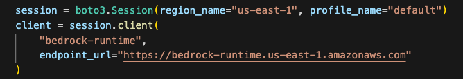
memory_client = MemoryClient(region_name="us-east-1")
memory = memory_client.create_memory_and_wait(
name="CustomerSupport",
description="Customer support conversations"
)
I can now use create_event to stores agent interactions into short-term memory:
memory_client.create_event(
    memory_id=memory.get("id"), # Identifies the memory store
    actor_id="user-123",        # Identifies the user
    session_id="session-456",   # Identifies the session
    messages=[
        ("Hi, ...", "USER"),
        ("I'm sorry to hear that...", "ASSISTANT"),
        ("get_orders(customer_id='123')", "TOOL"),
        . . .
    ]
)
I can load the most recent turns of a conversations from short-term memory using list_events:
conversations = memory_client.list_events(
    memory_id=memory.get("id"), # Identifies the memory store
    actor_id="user-123",        # Identifies the user
    session_id="session-456",   # Identifies the session
    max_results=5               # Number of most recent turns to retrieve
)
With this capability, the agent can maintain context during long sessions. But when a users come back with a new session, the conversation starts blank. Using long-term memory, the agent can personalize user experiences by retaining insights across multiple interactions.
To extract memories from a conversation, I can use built-in AgentCore Memory policies for user preferences, summarization, and semantic memory (to capture facts) or create custom policies for specialized needs. Data is stored encrypted using a namespace-based storage for data segmentation.
I change the previous code creating the memory store to include long-term capabilities by passing a semantic memory strategy. Note that an existing memory store can be updated to add strategies. In that case, the new strategies are applied to newer events.
memory = memory_client.create_memory_and_wait(
    name="CustomerSupport",
    description="Customer support conversations",
    strategies=[{
        "semanticMemoryStrategy": {
            "name": "semanticFacts",
            "namespaces": ["/facts/{actorId}"]
        }
    }]
)
After long-term memory has been configured for a memory store, calling create_event will automatically apply those strategies to extract information from the conversations. I can then retrieve memories extracted from the conversation using a semantic query:
memories = memory_client.retrieve_memories(
    memory_id=memory.get("id"),
    namespace="/facts/user-123",
    query="smartphone model"
)
In this way, I can quickly improve the user experience so that the agent remembers customer preferences and facts that are outside of the scope of the CRM and use this information to improve the replies.
Step 3 – Adding identity and access controls
Without proper identity controls, access from the agent to internal tools always uses the same access level. To follow security requirements, I integrate AgentCore Identity so that the agent can use access controls scoped to the user’s or agent’s identity context.
I set up an identity client and create a workload identity, a unique identifier that represents the agent within the AgentCore Identity system:
from bedrock_agentcore.services.identity import IdentityClient

identity_client = IdentityClient("us-east-1")
workload_identity = identity_client.create_workload_identity(name="my-agent")
Then, I configure the credential providers, for example:
google_provider = identity_client.create_oauth2_credential_provider(
    {
        "name": "google-workspace",
        "credentialProviderVendor": "GoogleOauth2",
        "oauth2ProviderConfigInput": {
            "googleOauth2ProviderConfig": {
                "clientId": "your-google-client-id",
                "clientSecret": "your-google-client-secret",
            }
        },
    }
)

perplexity_provider = identity_client.create_api_key_credential_provider(
    {
        "name": "perplexity-ai",
        "apiKey": "perplexity-api-key"
    }
)
I can then add the @requires_access_token Python decorator (passing the provider name, the scope, and so on) to the functions that need an access token to perform their activities.
Using this approach, the agent can verify the identity through the company’s existing identity infrastructure, operate as a distinct, authenticated identity, act with scoped permissions and integrate across multiple identity providers (such as Amazon Cognito, Okta, or Microsoft Entra ID) and service boundaries including AWS and third-party tools and services (such as Slack, GitHub, and Salesforce).
To offer robust and secure access controls while streamlining end-user and agent builder experiences, AgentCore Identity implements a secure token vault that stores users’ tokens and allows agents to retrieve them securely.
For OAuth 2.0 compatible tools and services, when a user first grants consent for an agent to act on their behalf, AgentCore Identity collects and stores the user’s tokens issued by the tool in its vault, along with securely storing the agent’s OAuth client credentials. Agents, operating with their own distinct identity and when invoked by the user, can then access these tokens as needed, reducing the need for frequent user consent.
When the user token expires, AgentCore Identity triggers a new authorization prompt to the user for the agent to obtain updated user tokens. For tools that use API keys, AgentCore Identity also stores these keys securely and gives agents controlled access to retrieve them when needed. This secure storage streamlines the user experience while maintaining robust access controls, enabling agents to operate effectively across various tools and services.
Step 4 – Expanding agent capabilities with AgentCore Gateway
Until now, all internal tools are simulated in the code. Many agent frameworks, including Strands Agents, natively support MCP to connect to remote tools. To have access to internal systems (such as CRM and order management) via an MCP interface, I use AgentCore Gateway.
With AgentCore Gateway, the agent can access AWS services using Smithy models, Lambda functions, and internal APIs and third-party providers using OpenAPI specifications. It employs a dual authentication model to have secure access control for both incoming requests and outbound connections to target resources. Lambda functions can be used to integrate external systems, particularly applications that lack standard APIs or require multiple steps to retrieve information.
AgentCore Gateway facilitates cross-cutting features that most customers would otherwise need to build themselves, including authentication, authorization, throttling, custom request/response transformation (to match underlying API formats), multitenancy, and tool selection.
The tool selection feature helps find the most relevant tools for a specific agent’s task. AgentCore Gateway brings a uniform MCP interface across all these tools, using AgentCore Identity to provide an OAuth interface for tools that do not support OAuth out of the box like AWS services.
Step 5 – Adding capabilities with AgentCore Code Interpreter and Browser tools
To answer to customer requests, the customer support agent needs to perform calculations. To simplify that, I use the AgentCode SDK to add access to the AgentCore Code Interpreter.
Similarly, some of the integrations required by the agent don’t implement a programmatic API but need to be accessed through a web interface. I give access to the AgentCore Browser to let the agent navigate those web sites autonomously.
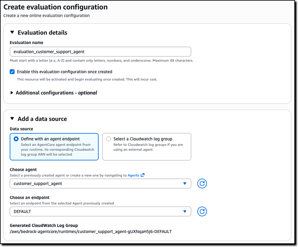
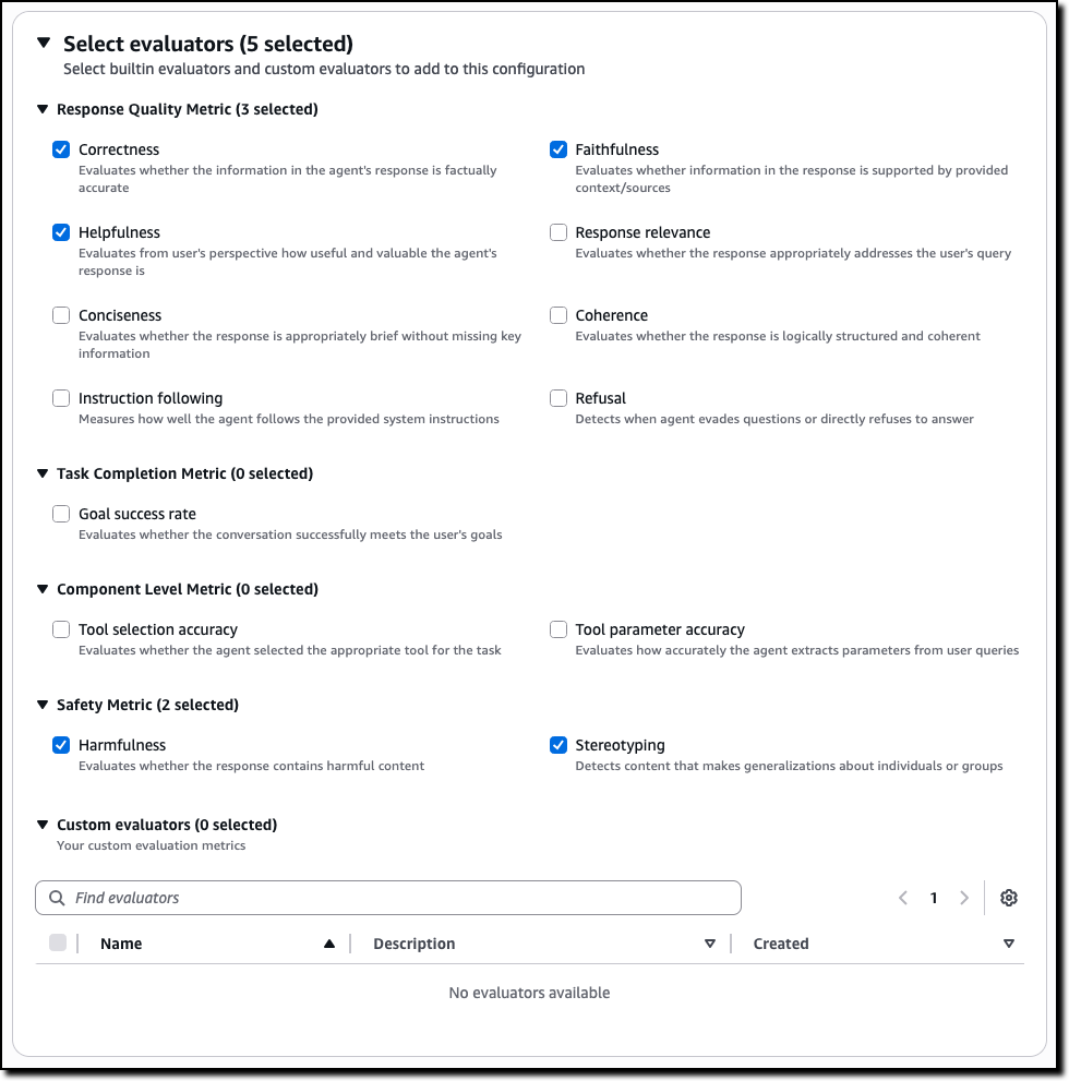
Step 6 – Gaining visibility with observability
Now that the agent is in production, I need visibility into its activities and performance. AgentCore provides enhanced observability to help developers effectively debug, audit, and monitor their agent performance in production. It comes with built-in dashboards to track essential operational metrics such as session count, latency, duration, token usage, error rates, and component-level latency and error breakdowns. AgentCore also gives visibility into an agent’s behavior by capturing and visualizing both the end-to-end traces, as well as “spans” that capture each step of the agent workflow including tool invocations, memory
The built-in dashboards offered by this service help reveal performance bottlenecks and identify why certain interactions might fail, enabling continuous improvement and reducing the mean time to detect (MTTD) and mean time to repair (MTTR) in case of issues.
AgentCore supports OpenTelemetry to help integrate agent telemetry data with existing observability platforms, including Amazon CloudWatch, Datadog, LangSmith, and Langfuse.
Step 7 – Conclusion
Through this journey, we transformed a local prototype into a production-ready system. Using AgentCore modular approach, we implemented enterprise requirements incrementally—from basic deployment to sophisticated memory, identity management, and tool integration—all while maintaining the existing agent code.
Things to know
Amazon Bedrock AgentCore is available in preview in US East (N. Virginia), US West (Oregon), Asia Pacific (Sydney), and Europe (Frankfurt). You can start using AgentCore services through the AWS Management Console , the AWS Command Line Interface (AWS CLI), the AWS SDKs, or via the AgentCore SDK.
You can try AgentCore services at no charge until September 16, 2025. Standard AWS pricing applies to any additional AWS Services used as part of using AgentCore (for example, CloudWatch pricing will apply for AgentCore Observability). Starting September 17, 2025, AWS will bill you for AgentCore service usage based on this page.
Whether you’re building customer support agents, workflow automation, or innovative AI-powered experiences, AgentCore provides the foundation you need to move from prototype to production with confidence.
To learn more and start deploying production-ready agents, visit the AgentCore documentation. For code examples and integration guides, check out the AgentCore samples GitHub repo.
Join the AgentCore Preview Discord server to provide feedback and discuss use cases. We’d like to hear from you!
— Danilo


![Screenshot of AI-DLC workspace detection phase showing the Amazon Q chat interface. The left sidebar displays the file tree with an 'aidlc-doc' folder highlighted. The main chat area shows the Inception Phase - Workspace Detection stage with explanatory text about analyzing the workspace. Five callout annotations explain: 1) Workflow creates aidlc-doc directory for storing AI-DLC generated artifacts; 2) The workflow tracks its progress in aidlc-metadata.json for error recovery and session continuity; 3) The audit.md file stores user's prompts; 4) Workflow highlights the AI-DLC phase and stage name with a clear heading for easy tracking; 5) Workflow loads detailed stage-level behavior files dynamically such that they don't consume the context window statically. At the bottom, a user approval prompt shows 'mkdir -p /Users/[...]/NewConsumerPortal/aidlc-docs' with the user asked to approve the 'mkdir' command.](https://d2908q01vomqb2.cloudfront.net/7719a1c782a1ba91c031a682a0a2f8658209adbf/2025/11/24/04_AI-DLC_workspace_detection-1.png)


 Nita Shah is an Analytics Specialist Solutions Architect at AWS based out of New York. She has been building data warehouse solutions for over 20 years and specializes in Amazon Redshift. She is focused on helping customers design and build enterprise-scale well-architected analytics and decision support platforms.
 Sushmita Barthakur is a Senior Data Solutions Architect at Amazon Web Services (AWS), supporting Strategic customers architect their data workloads on AWS. With a background in data analytics, she has extensive experience helping customers architect and build enterprise data lakes, ETL workloads, data warehouses and data analytics solutions, both on-premises and the cloud. Sushmita is based in Florida and enjoys traveling, reading and playing tennis.
 Jonathan Katz is a Principal Product Manager – Technical on the Amazon Redshift team and is based in New York. He is a Core Team member of the open source PostgreSQL project and an active open source contributor, including PostgreSQL and the pgvector project.
