Tag Archives: PyTorch on AWS

Accelerate CPU-based AI inference workloads using Intel AMX on Amazon EC2

Post Syndicated from Santosh Kumar original https://aws.amazon.com/blogs/compute/accelerate-cpu-based-ai-inference-workloads-using-intel-amx-on-amazon-ec2/

This post shows you how to accelerate your AI inference workloads by up to 76% using Intel Advanced Matrix Extensions (AMX) – an accelerator that uses specialized hardware and instructions to perform matrix operations directly on processor cores – on Amazon Elastic Compute Cloud (Amazon EC2) 8th generation instances. You’ll learn when CPU-based inference is cost-effective, how to enable AMX with minimal code changes, and which configurations deliver optimal performance for your models.

Many organizations find that CPU-based inference is more suitable for their production Artificial Intelligence/Machine Learning (AI/ML) workloads after evaluating factors like cost, operational complexity, and infrastructure compatibility. As more organizations deploy AI solutions, improving how models run on standard CPUs has become a critical cost control strategy for workloads where CPU inference provides the right balance of performance and economics.

IDC, a global market intelligence and advisory firm, projects that worldwide AI spending will reach $632 billion by 2028, growing at a 29% compound annual growth rate from 2024, with inference costs representing a significant portion of operational expenses. Deloitte, a leading professional services firm specializing in technology consulting and research, forecasts that inference – the running of AI models – will make up two-thirds of all AI compute by 2026, far exceeding initial training costs. This makes optimizing AI/ML inference on CPU crucial for controlling long-term AI/ML operational expenses.

At the core of AI inference workloads are matrix multiplication operations – the mathematical foundation of neural networks that drives computational demand. These matrix-heavy operations create a performance bottleneck for CPU-based inference, resulting in suboptimal performance for AI/ML workloads. This creates three key challenges for organizations: balancing cost optimization with performance requirements, meeting real-time latency demands, and scaling efficiently with variable workload demands. Intel’s Advanced Matrix Extensions (AMX) technology addresses these challenges by accelerating matrix operations directly on CPU cores, making CPU-based inference competitive and cost-effective.

AMX capabilities and architecture

AMX supports multiple data formats including BF16 which preserves the range of 32-bit floating point operations in half the space, INT8 maximizes throughput when accuracy can be slightly compromised, and FP16 offers a balance between the two. This flexibility lets you match precision to your specific needs.

Introduced in 2023 with 4th Generation Intel Xeon Scalable processors, AMX consists of eight 1KB tile registers (specialized on-chip memory for matrix data) and a Tile Matrix Multiply Unit (TMUL – dedicated hardware for matrix calculations) that enables processors to perform 2048 INT8 operations or 1024 BF16 operations per cycle. These tile registers provide efficient matrix storage, reducing memory access overhead and improving computational efficiency for matrix operations central to neural networks. For real-world customer workloads, this translates to significantly faster inference times for transformer models, recommendation systems, and natural language processing tasks, while reducing the total cost of ownership through improved resource utilization and lower infrastructure requirements.
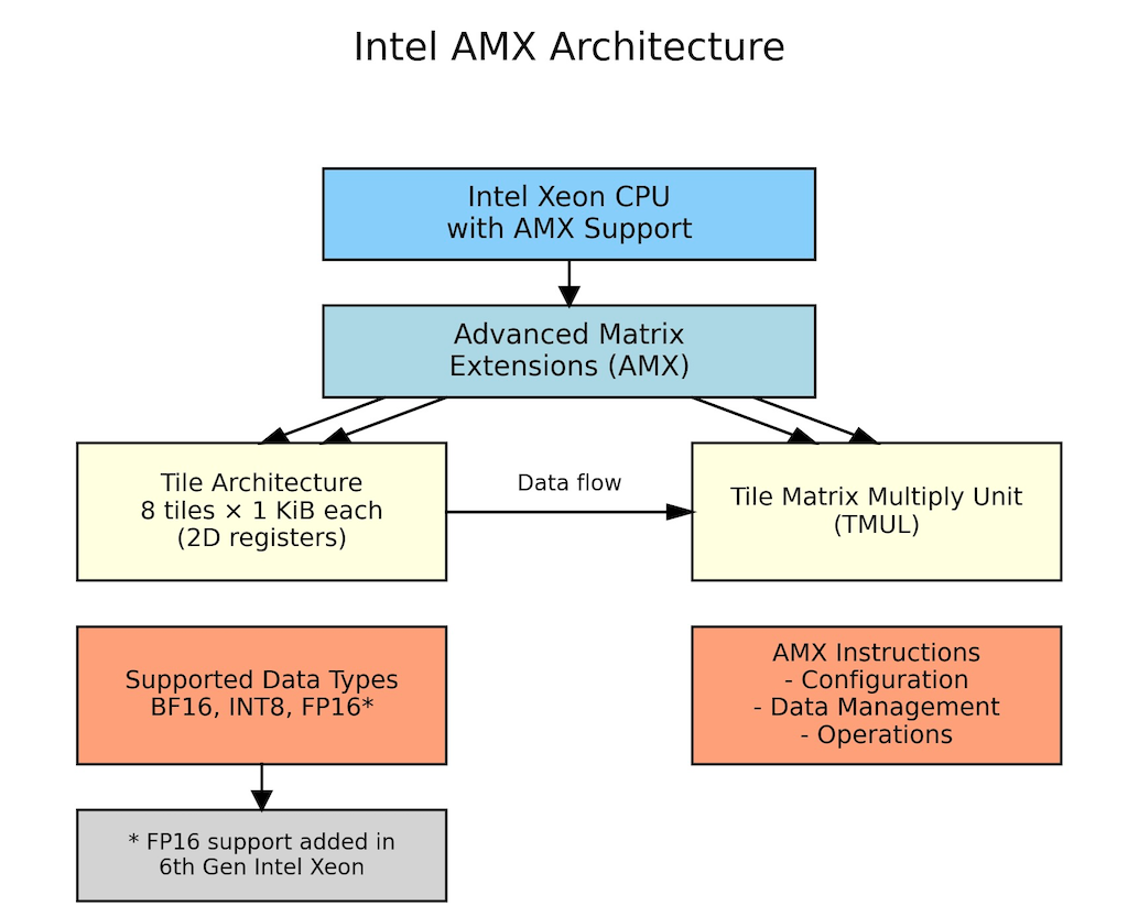
Architecture diagram of Intel Advanced Matrix Extensions (AMX) showing the key components: Intel Xeon CPU with AMX support, tile architecture with 8 tiles of 1 KiB each as 2D registers, Tile Matrix Multiply Unit (TMUL) with data flow between them, supported data types (BF16, INT8, FP16), and AMX instruction categories (Configuration, Data Management, Operations)

Figure 1: AMX Architecture showing AMX tile registers, processing units, and data flow within CPU core

Note: AMX operations, including tile setup and memory-to-tile data movement (which are handled automatically by the system), introduce small overhead that may outweigh benefits for smaller models or single-batch processing where insufficient matrix operations cannot amortize these costs, making batch size optimization critical for performance gains.

When to choose CPU inference with AMX

CPU inference with AMX acceleration benefits workloads including:

Batch processing and traditional ML: Content summarization, recommendation systems, and analytical workloads benefit from CPU’s cost efficiency and ability to handle sparse data structures and branching logic.

Small to medium-sized models: Models under 7B parameters and batch sizes of 8-16 samples achieve excellent performance through optimized threading, making CPUs ideal for applications like fraud detection and chatbots.

Variable demand workloads: E-commerce systems and applications with unpredictable traffic patterns can quickly scale CPU instances up or down based on demand, avoiding the fixed costs of dedicated accelerator hardware that sits idle during low-traffic periods.

Complex business logic: Applications like financial risk assessment and content moderation that need to combine ML predictions with business rules and conditional logic work well on CPUs, which handle mixed workloads better than specialized accelerators.

Implementation: AMX optimization with PyTorch

PyTorch, a popular open-source machine learning framework, includes built-in Intel optimizations through oneDNN (Intel’s Deep Neural Network library) that automatically use AMX when available. Setup requires installing dependencies and configuring environment variables for optimal performance.

Install dependencies

# Install transformers and torch
pip install torch transformers

Configure environment variables

These environment variables tell oneDNN library how to optimize your inference workload for AMX.

  1. Enable AMX instruction set (tells oneDNN to use AMX tiles for matrix operations):
    export DNNL_MAX_CPU_ISA=AVX512_CORE_AMX
  2. Optimize thread affinity (binds threads to CPU cores for better cache performance):
    export KMP_AFFINITY=granularity=fine,compact,1,0
  3. Use all available CPU cores for parallel processing:
    export OMP_NUM_THREADS=$(nproc)
  4. Cache compiled kernels (avoids recompilation overhead on subsequent runs):
    export ONEDNN_PRIMITIVE_CACHE_CAPACITY=4096
  5. Set default precision to BF16 (enables automatic AMX acceleration):
    export ONEDNN_DEFAULT_FPMATH_MODE=bf16
  6. (Optional) Enable verbose logging to verify AMX activation:
    export ONEDNN_VERBOSE=1

BF16 optimization example

With environment variables configured, implementing BF16 optimization requires minimal to no code changes. The following example demonstrates how PyTorch automatically leverages AMX tile registers for matrix operations when BF16 precision is used.

Note: This is a simplified example for demonstration purposes; adapt the code to your specific use case and requirements.

import torch
from transformers import AutoTokenizer, AutoModelForCausalLM
import time

# Load model and tokenizer from HuggingFace
model_name = "google/gemma-3-1b-it"

model_revision = "dcc83ea841ab6100d6b47a070329e1ba4cf78752"
tokenizer = AutoTokenizer.from_pretrained(
    model_name,
    revision=model_revision
)
model = AutoModelForCausalLM.from_pretrained(
    model_name,
    revision=model_revision
)
# Fix tokenizer padding issue for batch processing
if tokenizer.pad_token is None:
    tokenizer.pad_token = tokenizer.eos_token

# Enable BF16 precision for automatic AMX acceleration
model = model.to(dtype=torch.bfloat16)
model.eval()  # Set to inference mode

# Inference function with BF16 autocast
def run_optimized_inference(prompts):
    inputs = tokenizer(prompts, padding=True, 
                      return_tensors="pt")  # Tokenize input
    
    with torch.no_grad():  # Disable gradients for inference
        with torch.amp.autocast('cpu',
                               dtype=torch.bfloat16):  # BF16 autocast
            outputs = model.generate(
                **inputs,
                max_length=100,     # Set maximum sequence length 
                do_sample=False     # Use greedy decoding
            )
    return outputs

# Example usage with performance measurement
prompts = ["What are the benefits of cloud computing?"]
start_time = time.time()
results = run_optimized_inference(prompts)  # Run BF16-optimized inference
elapsed_time = time.time() - start_time
tokens_generated = len(results[0]) - len(tokenizer.encode(
    prompts[0]))  # Count new tokens

# Display results and performance metrics
print(tokenizer.decode(results[0], skip_special_tokens=True))
print(f"Latency: {elapsed_time*1000:.1f}ms, "
      f"Throughput: {tokens_generated/elapsed_time:.1f} "
      f"tokens/sec")

Performance benchmarks

To validate AMX performance benefits, we conducted benchmarks across multiple popular language models representing different use cases and model sizes.

Benchmarking methodology and environment

We tested two improvements: hardware generation advances (m8i vs m7i) and AMX optimization impact (FP32 vs BF16). This shows you both upgrade paths for your workloads.

  • Models tested: BigBird-RoBERTa-large (355M), Microsoft DialoGPT-large (762M), Google Gemma-3-1b-it (1B), DeepSeek-R1-Distill-Qwen-1.5B (1.5B), Llama-3.2-3B-Instruct (3B), YOLOv5 (tested with 30 images at ~1200×800 resolution with 5 iterations for each image)
  • Amazon EC2 instance types: m8i.4xlarge, m7i.4xlarge (8th & 7th gen general-purpose Amazon EC2 instances with 16 vCPUs and 64 GiB memory, both AMX-capable)
  • Batch sizes: 1, 8, 32 (number of input samples processed simultaneously in a single inference call)
  • Iterations: 5 runs per configuration
  • Comparison types:
    • Instance generation comparison (m8i vs m7i performance)
    • AMX optimization impact (32-bit floating-point (FP32) vs Brain Floating Point 16 (BF16) on same instance)
  • Optimizations: FP32 baseline vs BF16 AMX
  • Framework: PyTorch 2.8.0 (which has built-in Intel optimizations)
  • Region: AWS us-west-2
  • Measurement methodology: In our benchmarks, ‘inference latency’ represents the complete model inference execution time including input tokenization and full sequence generation (for generative models) or complete forward pass (for non-generative models). Each measurement is the average of 5 iterations after warm-up iterations, excluding model loading time. We use this metric because AMX’s matrix multiplication acceleration improves performance throughout the complete forward pass.

Note: Throughout this blog, FP32 refers to the default 32-bit floating-point precision, while BF16 refers to Brain Floating Point 16-bit precision with AMX acceleration enabled.

Disclaimer: Performance results are based on internal testing and may vary depending on specific workloads, configurations, and environments.

Detailed result: BigBird-RoBERTa-large

This benchmark represents document classification, content summarization, and text analysis workloads typical in batch processing where high throughput is desirable and offline inference scenarios where strict latency requirements are not critical.
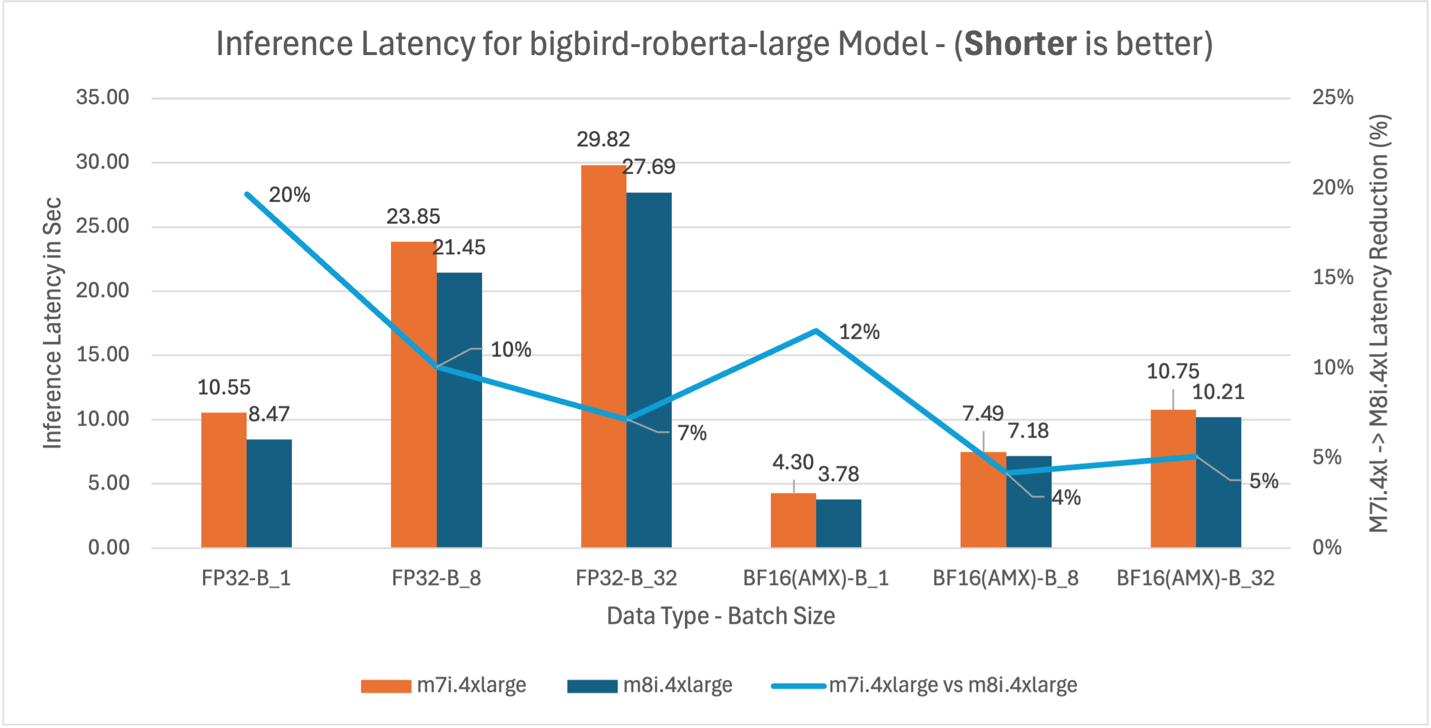
Bar chart comparing BigBird-RoBERTa-large inference latency between m7i and m8i instances with FP32 and BF16 precision across batch sizes 1, 8, and 32, showing 55-67% latency reduction with BF16 AMX.

Figure 2: m7i.4xlarge vs m8i.4xlarge inference latency comparison for model BigBird-RoBERTa-large (355M parameters)
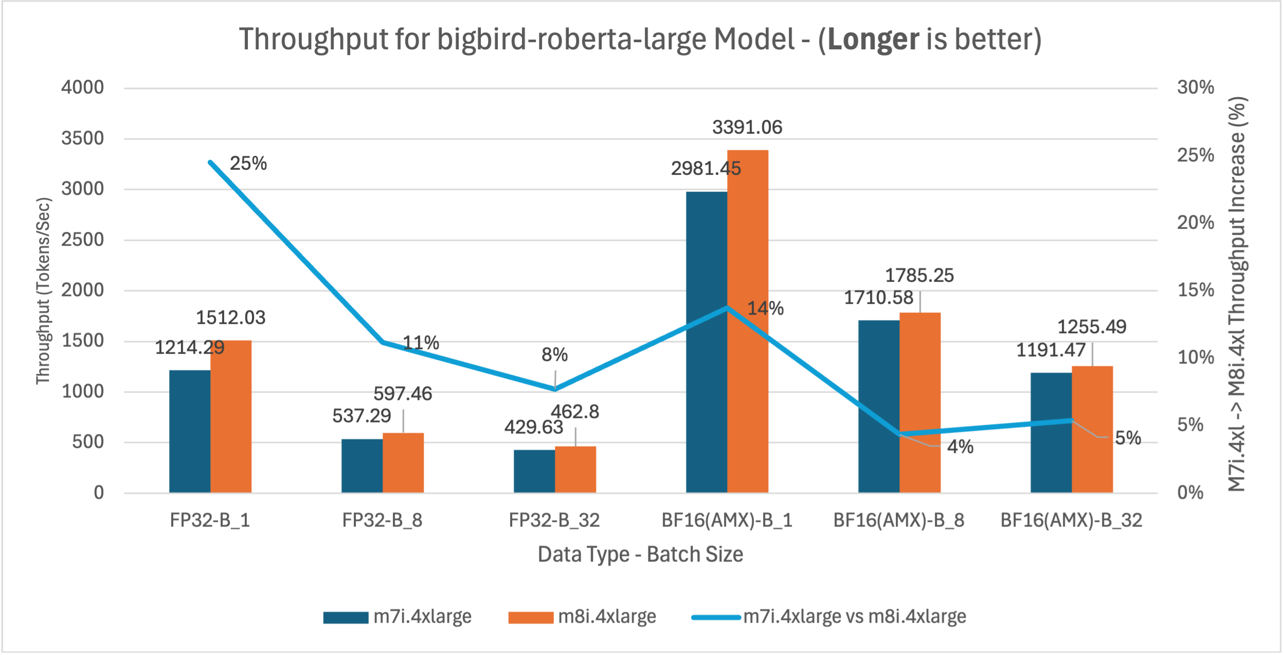
Bar chart comparing throughput for the BigBird-RoBERTa-large model between m7i.4xlarge and m8i.4xlarge instances across FP32 and BF16(AMX) data types at batch sizes 1, 8, and 32. m8i.4xlarge achieves 4–25% higher throughput, with the largest gain at FP32 batch size 1 (25%, from 1214.29 to 1512.03 tokens/sec). BF16(AMX) batch size 1 reaches the highest overall throughput at 3391.06 tokens/sec on m8i.4xlarge with a 14 % improvement over m7i.4xlarge. Throughput gains with BF16(AMX) are smaller at larger batch sizes (4–5%), as AMX overhead limits scaling for this smaller model.

Figure 3: m7i.4xlarge vs m8i.4xlarge throughput comparison for BigBird-RoBERTa-large model across batch sizes 1, 8, and 32
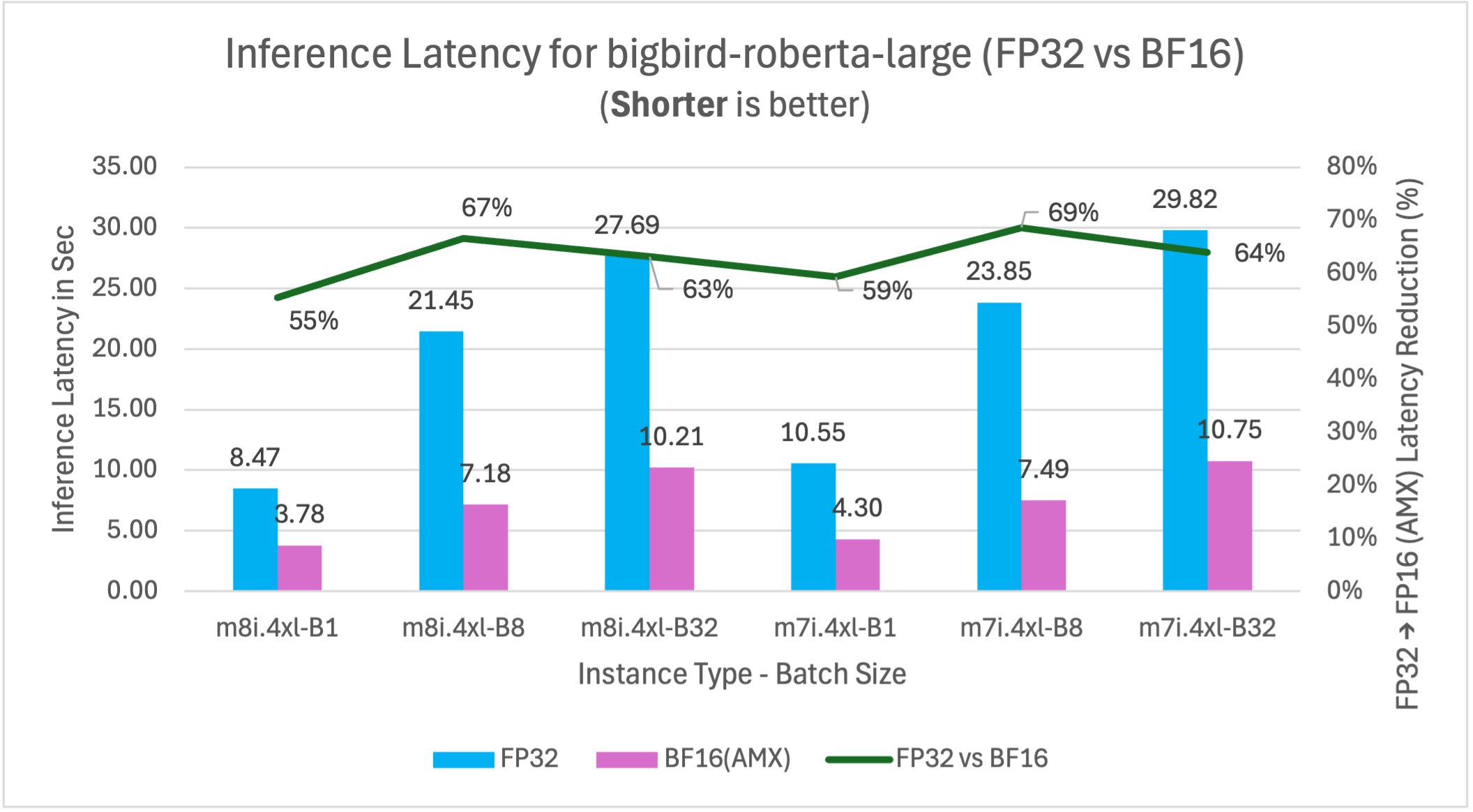
Bar chart comparing inference latency for bigbird-roberta-large between FP32 and BF16(AMX) data types on m8i.4xlarge and m7i.4xlarge instances at batch sizes 1, 8, and 32, showing BF16(AMX) reduces latency by 55–69% compared to FP32 across all configurations

Figure 4: FP32 vs BF16 inference latency comparison for model BigBird-RoBERTa-large (355M parameters) on m7i.4xlarge and m8i.4xlarge instances across batch sizes

BigBird-RoBERTa-large model benchmarking demonstrates three key performance improvements. Figure 2 shows m8i hardware delivers 4-20% latency reduction across batch sizes compared to m7i for both FP32 and BF16 with AMX, providing immediate benefits without application changes. With AMX and BF16, performance gains decrease at higher batch sizes as AMX overhead exceeds benefits for smaller models like BigBird-RoBERTa-large. Figure 3 validates these improvements with corresponding 4-25% throughput gains, enabling better resource utilization for production applications. Figure 4 demonstrates that enabling AMX with BF16 optimization provides the most significant impact, reducing m8i latency by 55-67% compared to non-AMX FP32 baseline, enabling 2-3x higher processing capacity and reduced compute costs.

The analysis above demonstrates the methodology for interpreting benchmark results using BigBird-RoBERTa-large as a representative example. The remaining models (DialoGPT-large, Gemma-3-1b-it, DeepSeek-R1-Distill-Qwen-1.5B, and Llama-3.2-3B-Instruct) follow identical testing procedures and exhibit similar performance patterns, with variations primarily in the magnitude of improvements based on model size and architecture. The comprehensive analysis of five models and their performance implications are synthesized in the following section.

Benchmarking result for additional models

To validate AMX’s effectiveness across diverse AI workloads, we benchmarked five additional models representing different use cases and model sizes. Each model follows the same testing methodology described above, with performance patterns showing how AMX benefits vary based on model architecture, parameter count, and batch size.

DialoGPT-large (762M) – Conversational AI

This benchmark represents conversational AI, chatbots, and real-time dialogue systems where low latency and consistent response times are critical for user experience.
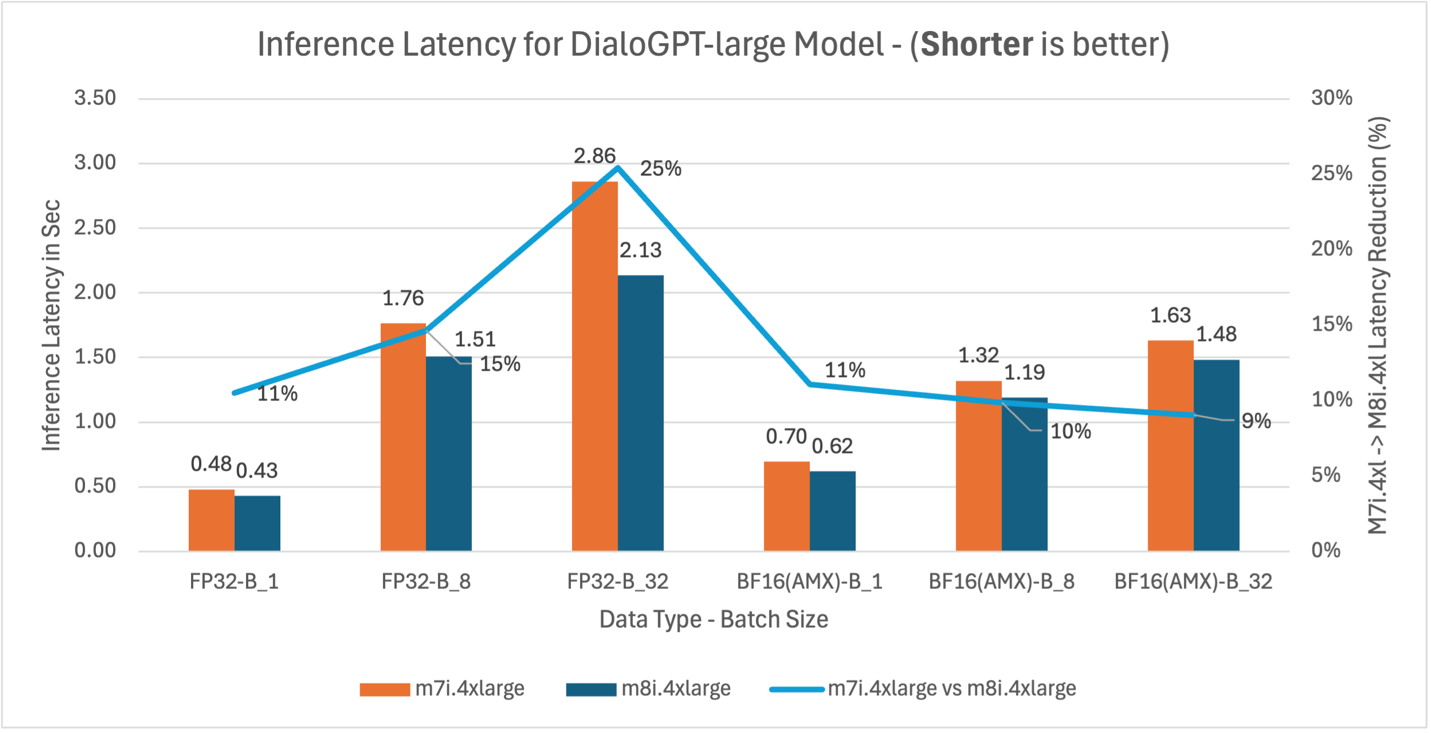
Bar chart comparing inference latency for the DialoGPT-large model between m7i.4xlarge and m8i.4xlarge instances across FP32 and BF16(AMX) data types at batch sizes 1, 8, and 32, showing m8i.4xlarge achieves 9– 25% latency reduction, with the largest improvement at FP32 batch size 32 (25%)

Figure 5: m7i.4xlarge vs m8i.4xlarge inference latency comparison for model DialoGPT-large (762M parameters)
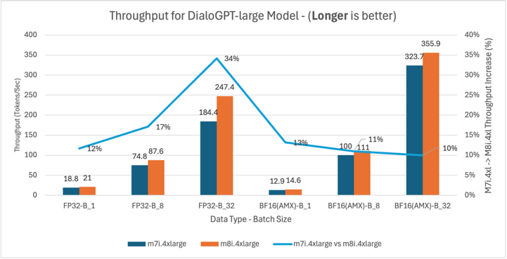
Bar chart comparing throughput for the DialoGPT-large model between m7i.4xlarge and m8i.4xlarge instances across FP32 and BF16(AMX) data types at batch sizes 1, 8, and 32, showing m8i.4xlarge achieves 10–34% higher throughput, with the largest gain at FP32 batch size 32 (34%) and BF16(AMX) batch size 32 reaching the highest overall throughput at 355.9 tokens/sec

Figure 6: m7i.4xlarge vs m8i.4xlarge throughput comparison for DialoGPT-large model across batch sizes 1, 8, and 32
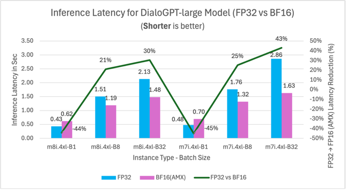
Bar chart comparing inference latency for DialoGPT-large between FP32 and BF16(AMX) data types on m8i.4xlarge and m7i.4xlarge instances at batch sizes 1, 8, and 32, showing BF16(AMX) increases latency at batch size 1 (negative improvement of -44% and -45%) but reduces latency at larger batch sizes, with up to 43% reduction at m7i.4xlarge batch size 32

Figure 7: FP32 vs BF16 inference latency comparison for model DialoGPT-large (762M parameters) on m7i.4xlarge and m8i.4xlarge instances across batch sizes

Gemma-3-1b-it (1B) – General Purpose

This benchmark represents general-purpose language understanding tasks, content generation, and smaller model deployments suitable for cost-sensitive applications and variable demand workloads.
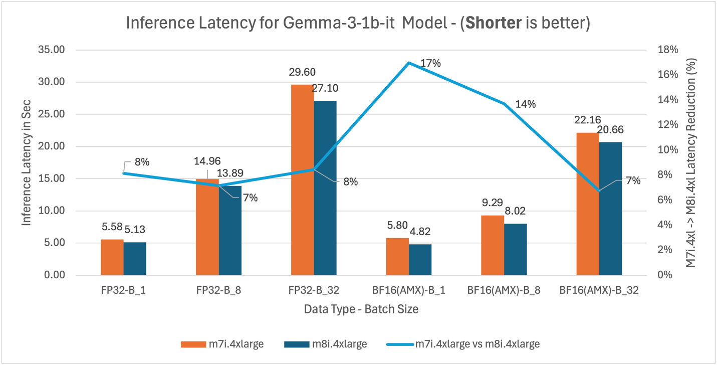
Bar chart comparing inference latency for the Gemma-3-1b-it model between m7i.4xlarge and m8i.4xlarge instances across FP32 and BF16(AMX) data types at batch sizes 1, 8, and 32, showing m8i.4xlarge achieves 7– 17% latency reduction, with the largest improvement at BF16(AMX) batch size 1 (17%)

Figure 8: M7i.4xlarge vs M8i.4xlarge inference latency comparison for model Gemma-3-1b-it (1B parameters)
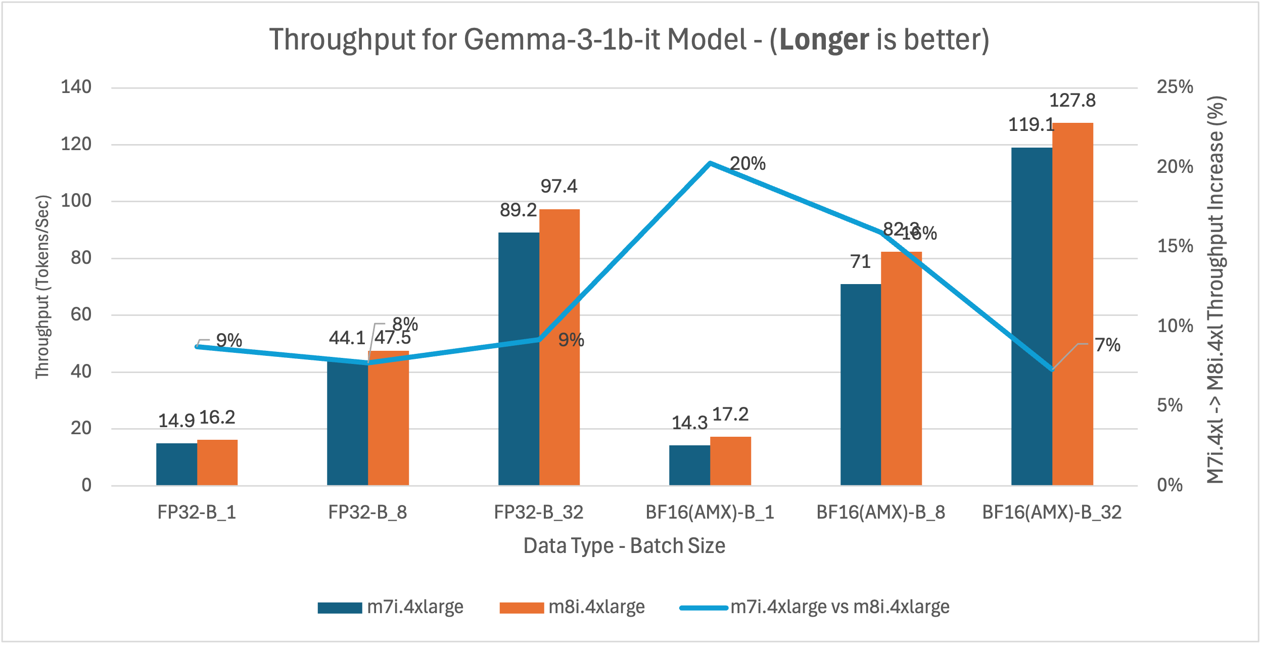
Bar chart comparing throughput for the Gemma-3-1b-it model between m7i.4xlarge and m8i.4xlarge instances across FP32 and BF16(AMX) data types at batch sizes 1, 8, and 32, showing m8i.4xlarge achieves 7–20% higher throughput, with the largest gain at BF16(AMX) batch size 1 (20%) and BF16(AMX) batch size 32 reaching the highest overall throughput at 127.8 tokens/sec

Figure 9: m7i.4xlarge vs m8i.4xlarge latency and throughput comparison for Gemma-3-1b-it across model batch sizes 1, 8, and 32
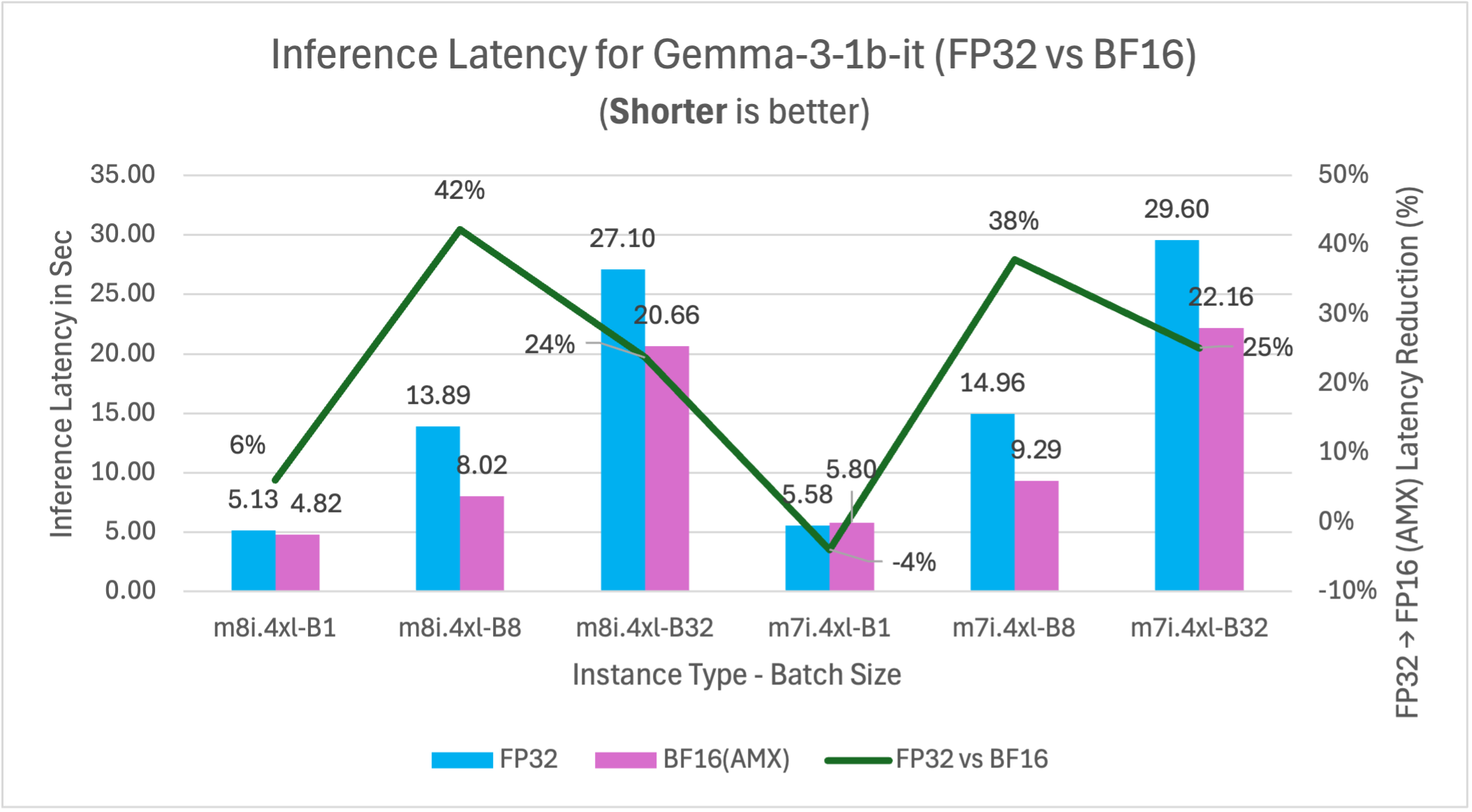
Bar chart comparing inference latency for Gemma-3-1b-it between FP32 and BF16(AMX) data types on m8i.4xlarge and m7i.4xlarge instances at batch sizes 1, 8, and 32, showing BF16(AMX) reduces latency by 24–42% at larger batch sizes but slightly increases latency at m7i.4xlarge batch size 1 (-4%), with the best improvement of 42% on m8i.4xlarge at batch size 8

Figure 10: FP32 vs BF16 inference latency comparison for model Gemma-3-1b-it (1B parameters) on m7i.4xlarge and m8i.4xlarge instances across batch sizes

DeepSeek-R1-Distill-Qwen-1.5B (1.5B) – Reasoning

This benchmark represents reasoning and analytical workloads, including complex decision-making systems, financial analysis, and applications requiring sophisticated logic processing.
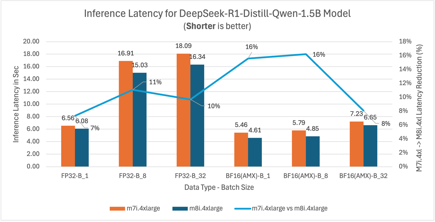
Bar chart comparing inference latency for the DeepSeek-R1-Distill-Qwen-1.5B model between m7i.4xlarge and m8i.4xlarge instances across FP32 and BF16(AMX) data types at batch sizes 1, 8, and 32, showing m8i.4xlarge achieves 7–16% latency reduction, with the largest improvements at BF16(AMX) batch sizes 1 and 8 (both 16%)

Figure 11: m7i.4xlarge vs m8i.4xlarge inference latency comparison for model DeepSeek-R1-Distill-Qwen-1.5B (1.5B parameters)
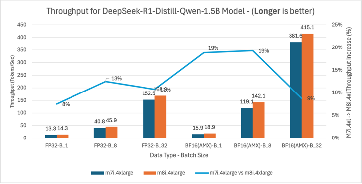
Bar chart comparing throughput for the DeepSeek-R1-Distill-Qwen-1.5B model between m7i.4xlarge and m8i.4xlarge instances across FP32 and BF16(AMX) data types at batch sizes 1, 8, and 32, showing m8i.4xlarge achieves 8–19% higher throughput, with the largest gains at BF16(AMX) batch sizes 1 and 8 (both 19%) and BF16(AMX) batch size 32 reaching the highest overall throughput at 415.1 tokens/sec

Figure 12: m7i.4xlarge vs m8i.4xlarge latency and throughput comparison for DeepSeek-R1-Distill-Qwen-1.5B model across batch sizes 1, 8, and 32
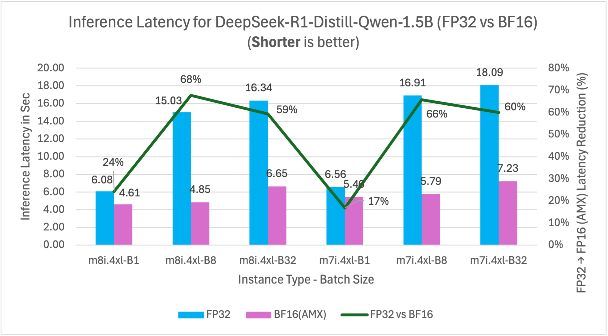
Bar chart comparing inference latency for DeepSeek-R1-Distill-Qwen-1.5B between FP32 and BF16(AMX) data types on m8i.4xlarge and m7i.4xlarge instances at batch sizes 1, 8, and 32, showing BF16(AMX) reduces latency by 17–68% across all configurations, with the largest improvement of 68% on m8i.4xlarge at batch size 8 and consistently strong reductions of 59–66% at larger batch sizes

Figure 13: FP32 vs BF16 inference latency comparison for model DeepSeek-R1-Distill-Qwen-1.5B (1.5B parameters) on m7i.4xlarge and m8i.4xlarge instances across batch sizes

Llama-3.2-3B-Instruct (3B) – Large model

This benchmark represents larger model deployments for complex instruction-following tasks, advanced content generation, and applications requiring higher model capacity while maintaining cost efficiency.
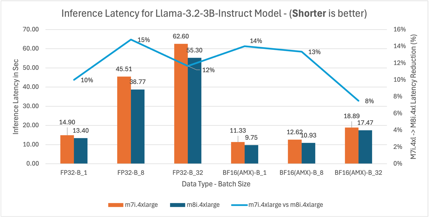
Bar chart comparing inference latency for the Llama-3.2-3B-Instruct model between m7i.4xlarge and m8i.4xlarge instances across FP32 and BF16(AMX) data types at batch sizes 1, 8, and 32, showing m8i.4xlarge achieves 8–15% latency reduction, with the largest improvement at FP32 batch size 8 (15%) and consistent gains of 12–14% with BF16(AMX) at smaller batch sizes

Figure 14: m7i.4xlarge vs m8i.4xlarge inference latency comparison for model Llama-3.2-3B-Instruct (3B parameters)
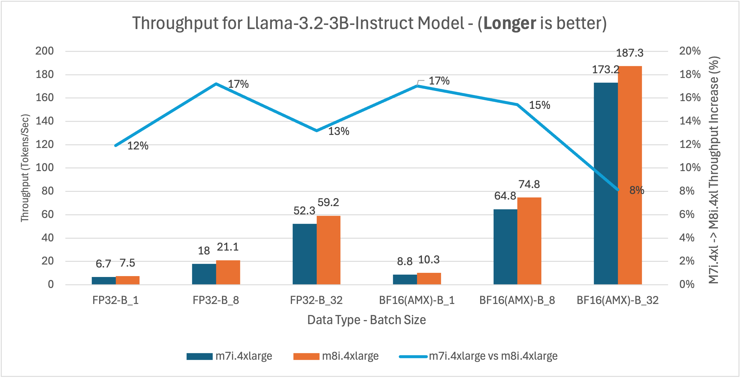
Bar chart comparing throughput for the Llama-3.2-3B-Instruct model between m7i.4xlarge and m8i.4xlarge instances across FP32 and BF16(AMX) data types at batch sizes 1, 8, and 32, showing m8i.4xlarge achieves 8– 17% higher throughput, with the largest gains at FP32 batch size 8 and BF16(AMX) batch size 1 (both 17%) and BF16(AMX) batch size 32 reaching the highest overall throughput at 187.3 tokens/sec

Figure 15: m7i.4xlarge vs m8i.4xlarge latency and throughput comparison for Llama-3.2-3B-Instruct model across batch sizes 1, 8, and 32
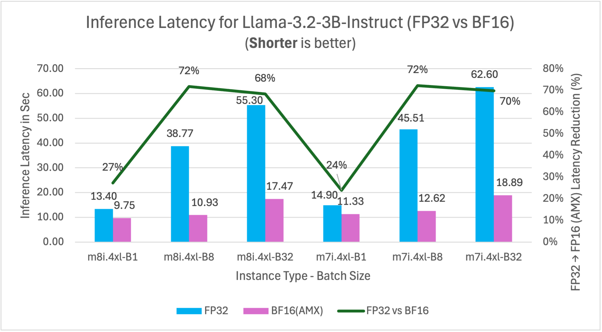
Bar chart comparing inference latency for Llama-3.2-3B-Instruct between FP32 and BF16(AMX) data types on m8i.4xlarge and m7i.4xlarge instances at batch sizes 1, 8, and 32, showing BF16(AMX) reduces latency by 24–72% across all configurations, with the largest improvements of 72% on both m8i.4xlarge batch size 8 and m7i.4xlarge batch size 8, and consistently strong reductions of 68–70% at batch size 32

Figure 16: FP32 vs BF16 inference latency comparison for model Llama-3.2-3B-Instruct (3B parameters) on m7i.4xlarge and m8i.4xlarge instances across batch sizes

Yolov5 – Computer vision model

This benchmark represents computer vision workloads including object detection, image classification, and real-time video processing applications where consistent throughput is important for production deployments.

Instance type Inference latency in Sec (Processing time per image)

Throughput

(Image processed per sec)

FP32 BF16 FP32 BF16
m8i.4xlarge 0.034 0.029 29.23 34.63
m7i.4xlarge 0.038 0.031 26.39 32.28
m8i improvement 10.5% 6.5% 10.8% 7.3%

Key insights: m8i instances deliver 7-11% better performance than m7i across both precision formats. Combining hardware upgrade with AMX optimization, m8i with BF16 delivers up to 24% lower latency and 31% higher throughput compared to m7i with FP32.

Benchmark result summary

The detailed graphs above demonstrate consistent performance patterns across tested models. Key findings:

M8i vs M7i instance performance

m8i instances deliver 9-14% average and up to 20% better performance than m7i across the tested models through hardware advances: up to 4.6x larger L3 cache, higher base frequencies, up to 2.5x higher DDR5 bandwidth, and enhanced AMX execution with FP16 support.

Model Use Case m8i average latency improvement*
BigBird-RoBERTa-large (355M) Document analysis 10%
DialoGPT-large (762M) Conversational AI 14%
Gemma-3-1b-it (1B) General purpose 10%
DeepSeek-R1 (1.5B) Reasoning tasks 11%
Llama-3.2-3B (3B) Large model deployment 12%
YOLOv5 Computer vision 9%

* Average across all tested configurations (FP32 and BF16 at batch sizes 1, 8, and 32)

AMX acceleration impact (FP32 vs BF16)

BF16 precision with AMX delivers 21-72% performance improvements at batch sizes of 8 and above compared to FP32 baseline on the same instance type. These results compare FP32 vs BF16 performance on m8i.4xlarge, with performance gains varying by model size and batch configuration. Larger batch sizes show greater AMX benefits.

Model Latency improvement (%)
Batch 1 Batch 8 Batch 32
BigBird-RoBERTa-large 55 67 63
DialoGPT-large – 44* 21 30
Gemma-3-1b-it 6 42 24
DeepSeek-R1 24 68 59
Llama-3.2-3B 27 72 68

* At batch size 1, DialoGPT-large’s autoregressive decoding generates tokens sequentially, producing many small matrix operations where AMX tile setup overhead exceeds the acceleration benefit. At batch sizes 8 and above, multiple sequences are processed in parallel, creating larger matrix operations that amortize this overhead and deliver 21-30% improvement.

Performance patterns by batch size

Larger models (1B+ parameters) show consistently better AMX performance across the tested batch sizes:

  • Batch size 1: Mixed results – larger models show 6-27% improvement, smaller models may experience AMX overhead
  • Batch size 8: Strong performance gains of 21-72% across the tested models, with larger models showing greater benefits
  • Batch size 32: Significant improvements of 24-68% for most models, demonstrating AMX’s batch processing strength

Batch size optimization guidelines

AMX performance scales with batch size, with optimal range varies by model size. Performance saturates beyond batch 16 due to hardware limits including memory bandwidth and compute bottlenecks.

Model Size Performance Gain Recommended Batch Size Notes
<1B parameters 21-67% 8-32 Batch 1 results vary by architecture*
1-2B parameters 42-68% 4-16 6-24% gains even at batch 1
3B+ parameters 27-72% 1-8 Benefits across batch sizes

* Encoder models (BigBird) show 55% gains at batch 1; autoregressive models (DialoGPT) may experience overhead.

Combined performance benefits

When we combine AMX optimization with 8th generation instances (m8i), the performance improvements compound significantly. For example, Llama-3.2-3B-Instruct running with BF16 AMX on m8i instances can achieve up to 76% better performance compared to FP32 inference on m7i instances at optimal batch sizes (batch 8: m7i FP32 45.51s vs m8i BF16 10.93s = 76% improvement; batch 32: m7i FP32 62.60s vs m8i BF16 17.47s = 72% improvement).

Throughput scaling

Across the tested models, throughput (tokens/sec) increases proportionally with latency reduction. This consistent relationship demonstrates that AMX optimizations translate directly to improved inference efficiency.

Price-Performance Analysis: Gemma-3-1b-it Model

While m8i.4xlarge instances are priced slightly higher than m7i.4xlarge ($0.847 vs $0.806 per hour in us-west-2), they deliver superior price-performance. To illustrate the economic benefits, we analyzed cost per 1 million tokens using Gemma-3-1b-it as a representative example. M8i delivers up to 13% better price-performance over m7i through hardware generation advances, with both instances running BF16 AMX.

Batch Size Data Type m7i.4xlarge m8i.4xlarge Price-Performance improvement
Throughput
(tokens/sec)
$ per 1M token Throughput
(tokens/sec)
$ per 1M token
1 BF16(AMX) 14.3 $15.66 17.2 $13.67 13%
8 BF16(AMX) 71 $3.16 82.3 $2.86 9%
32 BF16(AMX) 119.1 $1.88 127.8 $1.84 2%

Combining the hardware upgrade with BF16 AMX optimization delivers up to 44% better price-performance compared to FP32 on m7i.

Batch Size m8i.4xlarge m7i.4xlarge


Price-Performance improvement

Data Type Throughput
(tokens/sec)
$ per 1M token Data Type Throughput
(tokens/sec)
$ per 1M token
1 BF16(AMX) 17.2 $13.67 FP32 14.9 $15.03 9%
8 BF16(AMX) 82.3 $2.86 FP32 44.1 $5.08 44%
32 BF16(AMX) 127.8 $1.84 FP32 89.2 $2.51 27%

Key findings from the price-performance analysis:

  • Combined optimization delivers up to 44% better price-performance: m8i with AMX and BF16 outperforms m7i with FP32 at batch size 8 – consistent with our batch size optimization guidelines where batch sizes of 4-16 deliver optimal results for 1B models like Gemma-3-1b-it, achieving $2.86 per 1M tokens for applications like chatbots and fraud detection.
  • Larger batches maximize cost efficiency: Batch size 32 reduces costs further to $1.84 per 1M tokens, a 27% improvement over m7i FP32 – ideal for throughput-oriented workloads like content summarization and recommendation systems where latency requirements are flexible.

Production deployment recommendation

  • BF16 AMX: Delivers 21-72% performance improvements at recommended batch sizes while maintaining model accuracy, making it suitable for production workloads including fraud detection systems, content moderation, and real-time recommendation engines
  • Batch processing: Target batch sizes of 4-16 based on your use case – smaller batches (1-4) for latency-sensitive applications like chatbots, larger batches (8-16) for throughput-focused scenarios like document analysis and offline processing
  • Instance selection: m8i instances provide consistent 9-14% performance improvements over m7i, delivering immediate ROI for existing CPU inference workloads without requiring application changes
  • Model size consideration: Larger models (1B+ parameters) show better AMX utilization across batch sizes, making them ideal candidates for m8i deployment in complex reasoning and content generation applications

Conclusion and next steps

By using Intel AMX on Amazon EC2 8th generation instances, you can achieve substantial performance improvements for AI inference workloads. Our benchmarks demonstrate up to 72% performance improvements across popular language models, making CPU inference more competitive for batch processing, real-time applications, recommender systems, and variable demand workloads while delivering substantial cost savings through improved resource utilization.

Key takeaways:

  • BF16 AMX optimization delivers up to 72% performance improvements across model sizes, with batch 8 showing 21-72% gains and batch 32 showing 24-68% gains
  • Batch sizes of 4-8 provide optimal performance for most models—DialoGPT achieves 21% improvement in latency at batch 8, while Llama-3.2-3B achieves 72% improvement
  • 8th generation instances deliver up to 14% performance improvements over m7i across the tested workloads
  • Combined optimizations (m8i + BF16 AMX) can achieve compound performance improvements up to 76% in optimal configurations (vs m7i FP32), making CPU inference highly competitive for cost-sensitive applications
  • M8i instances deliver up to 13% better price-performance vs m7i (lower cost per 1M tokens), based on our analysis of the Gemma-3-1b-it model
  • Proper environment configuration is critical for AMX activation

You can implement these optimizations immediately. AMX hardware acceleration combined with PyTorch’s Intel-specific enhancements requires configuring environment variables while delivering substantial speed gains. Begin with BF16 optimization on your existing models, then explore INT8 quantization for additional gains.

Next steps:

  1. Launch an Intel based Amazon EC2 8th generation instance (m8i.4xlarge)
  2. Install PyTorch (includes built-in Intel optimizations)
  3. Configure AMX environment variables
  4. Measure performance improvements
  5. Scale your optimized inference workloads

Additional resources

AWS Weekly Roundup — Claude 3 Haiku in Amazon Bedrock, AWS CloudFormation optimizations, and more — March 18, 2024

Post Syndicated from Antje Barth original https://aws.amazon.com/blogs/aws/aws-weekly-roundup-claude-3-haiku-in-amazon-bedrock-aws-cloudformation-optimizations-and-more-march-18-2024/

Storage, storage, storage! Last week, we celebrated 18 years of innovation on Amazon Simple Storage Service (Amazon S3) at AWS Pi Day 2024. Amazon S3 mascot Buckets joined the celebrations and had a ton of fun! The 4-hour live stream was packed with puns, pie recipes powered by PartyRock, demos, code, and discussions about generative AI and Amazon S3.

AWS Pi Day 2024

AWS Pi Day 2024 — Twitch live stream on March 14, 2024

In case you missed the live stream, you can watch the recording. We’ll also update the AWS Pi Day 2024 post on community.aws this week with show notes and session clips.

Last week’s launches
Here are some launches that got my attention:

Anthropic’s Claude 3 Haiku model is now available in Amazon Bedrock — Anthropic recently introduced the Claude 3 family of foundation models (FMs), comprising Claude 3 Haiku, Claude 3 Sonnet, and Claude 3 Opus. Claude 3 Haiku, the fastest and most compact model in the family, is now available in Amazon Bedrock. Check out Channy’s post for more details. In addition, my colleague Mike shows how to get started with Haiku in Amazon Bedrock in his video on community.aws.

Up to 40 percent faster stack creation with AWS CloudFormation — AWS CloudFormation now creates stacks up to 40 percent faster and has a new event called CONFIGURATION_COMPLETE. With this event, CloudFormation begins parallel creation of dependent resources within a stack, speeding up the whole process. The new event also gives users more control to shortcut their stack creation process in scenarios where a resource consistency check is unnecessary. To learn more, read this AWS DevOps Blog post.

Amazon SageMaker Canvas extends its model registry integrationSageMaker Canvas has extended its model registry integration to include time series forecasting models and models fine-tuned through SageMaker JumpStart. Users can now register these models to the SageMaker Model Registry with just a click. This enhancement expands the model registry integration to all problem types supported in Canvas, such as regression/classification tabular models and CV/NLP models. It streamlines the deployment of machine learning (ML) models to production environments. Check the Developer Guide for more information.

For a full list of AWS announcements, be sure to keep an eye on the What’s New at AWS page.

Other AWS news
Here are some additional news items, open source projects, and Twitch shows that you might find interesting:

AWS Build On Generative AIBuild On Generative AI — Season 3 of your favorite weekly Twitch show about all things generative AI is in full swing! Streaming every Monday, 9:00 US PT, my colleagues Tiffany and Darko discuss different aspects of generative AI and invite guest speakers to demo their work. In today’s episode, guest Martyn Kilbryde showed how to build a JIRA Agent powered by Amazon Bedrock. Check out show notes and the full list of episodes on community.aws.

Amazon S3 Connector for PyTorch — The Amazon S3 Connector for PyTorch now lets PyTorch Lightning users save model checkpoints directly to Amazon S3. Saving PyTorch Lightning model checkpoints is up to 40 percent faster with the Amazon S3 Connector for PyTorch than writing to Amazon Elastic Compute Cloud (Amazon EC2) instance storage. You can now also save, load, and delete checkpoints directly from PyTorch Lightning training jobs to Amazon S3. Check out the open source project on GitHub.

AWS open source news and updates — My colleague Ricardo writes this weekly open source newsletter in which he highlights new open source projects, tools, and demos from the AWS Community.

Upcoming AWS events
Check your calendars and sign up for these AWS events:

AWS at NVIDIA GTC 2024 — The NVIDIA GTC 2024 developer conference is taking place this week (March 18–21) in San Jose, CA. If you’re around, visit AWS at booth #708 to explore generative AI demos and get inspired by AWS, AWS Partners, and customer experts on the latest offerings in generative AI, robotics, and advanced computing at the in-booth theatre. Check out the AWS sessions and request 1:1 meetings.

AWS SummitsAWS Summits — It’s AWS Summit season again! The first one is Paris (April 3), followed by Amsterdam (April 9), Sydney (April 10–11), London (April 24), Berlin (May 15–16), and Seoul (May 16–17). AWS Summits are a series of free online and in-person events that bring the cloud computing community together to connect, collaborate, and learn about AWS.

AWS re:InforceAWS re:Inforce — Join us for AWS re:Inforce (June 10–12) in Philadelphia, PA. AWS re:Inforce is a learning conference focused on AWS security solutions, cloud security, compliance, and identity. Connect with the AWS teams that build the security tools and meet AWS customers to learn about their security journeys.

You can browse all upcoming in-person and virtual events.

That’s all for this week. Check back next Monday for another Weekly Roundup!

— Antje

This post is part of our Weekly Roundup series. Check back each week for a quick roundup of interesting news and announcements from AWS!

New – Profile Your Machine Learning Training Jobs With Amazon SageMaker Debugger

Post Syndicated from Julien Simon original https://aws.amazon.com/blogs/aws/profile-your-machine-learning-training-jobs-with-amazon-sagemaker-debugger/

Today, I’m extremely happy to announce that Amazon SageMaker Debugger can now profile machine learning models, making it much easier to identify and fix training issues caused by hardware resource usage.

Despite its impressive performance on a wide range of business problems, machine learning (ML) remains a bit of a mysterious topic. Getting things right is an alchemy of science, craftsmanship (some would say wizardry), and sometimes luck. In particular, model training is a complex process whose outcome depends on the quality of your dataset, your algorithm, its parameters, and the infrastructure you’re training on.

As ML models become ever larger and more complex (I’m looking at you, deep learning), one growing issue is the amount of infrastructure required to train them. For instance, training BERT on the publicly available COCO dataset takes well over six hours on a single p3dn.24xlarge instance, even with its eight NVIDIA V100 GPUs. Some customers like autonomous vehicle companies deal with much larger datasets, and train object detection models for several days.

When a complex training job takes this long, the odds that something goes wrong and ruins it are pretty high, not only wasting time and money but also causing lots of frustration. Important work needs to be put on the back burner while you investigate, figure out the root cause, try to fix it, and then run your training job again. Often, you’ll have to iterate quite a few times to nail the problem.

Depending on the ML framework that you use, and sometimes on its version, you may or may not be able to use existing framework-specific tools. Often, you’ll have to build and maintain your own bespoke tools. Even for experienced practitioners, this is a lot of hard work. For regular developers like me, this is an utterly daunting task.

Introducing Model Profiling in Amazon SageMaker Debugger
Launched last year at AWS re:Invent, Amazon SageMaker Debugger is a capability of Amazon SageMaker that automatically identifies complex issues developing in ML training jobs. These include loss not decreasing, exploding gradients, and more.

Now, SageMaker Debugger can also monitor hardware resource usage, and allows you to profile your training job to help you correlate resource usage to ML operations in your training script. Thus, you’ll be able to resolve performance issues much quicker, and iterate through your training job much faster.

Chaim Rand, ML Algorithm Developer at Mobileye, an Intel company building automated driving and driver assistance systems, had the opportunity to work with the new profiling capabilities, and here’s what he told us: “Many of the assisted driving and autonomous vehicle technologies that we develop at Mobileye, rely on training deep neural network models to detect a wide variety of road artifacts, including vehicles, pedestrians, speed bumps, road signs and more. Often, these models train on extremely large datasets, on multiple machines, and for periods of up to several days. For us, at Mobileye, it is imperative that we have a toolkit of advanced performance profiling capabilities, for analyzing the flow of data across the network, CPU, and GPU resources, and for pinpointing performance issues. The profiling functionality in SageMaker Debugger provides just that, taking performance profiling out of the domain of a few specialized experts, and empowering our algorithm developers to maximize training resource utilization, accelerate model convergence, and reduce cost.

At launch, the new profiling capability of SageMaker Debugger is available for TensorFlow 2.x and PyTorch 1.x. All you have to do is to train with the corresponding built-in frameworks in Amazon SageMaker. Distributed training is supported out of the box.

Setting a single parameter in your SageMaker estimator, and without any change to your training code, you can enable the collection of infrastructure and model metrics such as:

  • CPU and GPU,
  • RAM and GPU RAM,
  • Network I/O,
  • Storage I/O (local storage and Pipe Mode),
  • Python metrics,
  • Data loading time,
  • Time spent in ML operators running on CPU and GPU,
  • Distributed training metrics for Horovod,
  • and many more.

In addition, you can visualize how much time is spent in different phases, such as preprocessing, training loop, and postprocessing. If needed, you can drill down on each training epoch, and even on each function in your training script.

By default, metrics are collected every 500ms, and you can also set this value to 100ms, 200ms, 1s, 5s, and 1min. For finer-grained analysis, you can also enable and disable profiling explicitly in your training code, only capturing metrics for specific parts.

While your training job is running, you can easily visualize these metrics in Amazon SageMaker Studio, our web-based integrated development environment for ML. As you would expect, all data is also available through the SageMaker Debugger API, and you can retrieve it to build your own graphs.

Running in parallel of the training job, an Amazon SageMaker Processing analyzes captured data, builds graphs, and generates a report providing insights on potential problems. This doesn’t require any work on your part, as this analysis runs inside a built-in container on fully managed infrastructure.

Now, let’s run a demo with PyTorch, where we’ll profile a ResNet-50 image classification model training on the CIFAR-10 dataset.

Profiling a Training Job with Amazon SageMaker Debugger
All it takes to enable profiling on your training job is an extra parameter in your SageMaker estimator. You don’t need to change a line in your training code. By default, SageMaker Debugger uses a set of built-in profiling rules looking for unwanted conditions that could develop during training, such as low GPU utilization. On top of reporting these conditions, SageMaker Debugger also triggers events in CloudWatch Events. For example, I could use them to run a AWS Lambda function that automatically stops inefficient training jobs.

First, I create a profiling configuration capturing data every 500ms. Optionally, I could select a training step interval if I wanted to profile only a certain portion of the job.

import sagemaker
from sagemaker.profiler import ProfilerConfig 
profiler_config = ProfilerConfig(profiling_interval_millis=500)

Then, I pass this configuration to my PyTorch Estimator, training on an ml.p3.8xlarge instance equipped with 4 NVIDIA V100 GPUs.

from sagemaker.pytorch import PyTorch
estimator = PyTorch(
    role=sagemaker.get_execution_role(),
    instance_count=1,
    instance_type='ml.p3.8xlarge',
    entry_point='train_pt.py',
    framework_version='1.5.0',
    hyperparameters={"batch_size":512, "epochs":10},
    profiler_config=profiler_config)

Then, I launch the training job as usual. Once the job is running, profiling data is captured and stored in S3.

path = estimator.latest_job_profiler_artifacts_path()
print(path)
s3://sagemaker-us-east-2-123456789012/pt-train-pt-2020-11-17-17-38-43-231/profiler-output

Using the SageMaker SDK, I can retrieve and count profiling events.

from smdebug.profiler.system_metrics_reader import S3SystemMetricsReader
system_metrics_reader = S3SystemMetricsReader(path)
system_metrics_reader.refresh_event_file_list()
last_timestamp = system_metrics_reader.get_timestamp_of_latest_available_file()
events = system_metrics_reader.get_events(0, last_timestamp)
print("Found", len(events), "recorded system metric events. Latest recorded event:", last_timestamp)
Found 411853 recorded system metric events. Latest recorded event: 1605620280000000

Of course, I could parse and analyze these profiling events, build my own graphs, and so on. Instead, let’s visualize them in near real-time in SageMaker Studio.

While my training job is still running, I locate it in SageMaker Studio, and I right-click “Open Debugger for insights”.

SageMaker screenshot

This opens a new tab, and I select the “Nodes” panel where I can see details statistics for each instance in my training job. So, how’s my training job doing? Feel free to click on the image below to zoom in.

SageMaker screenshot

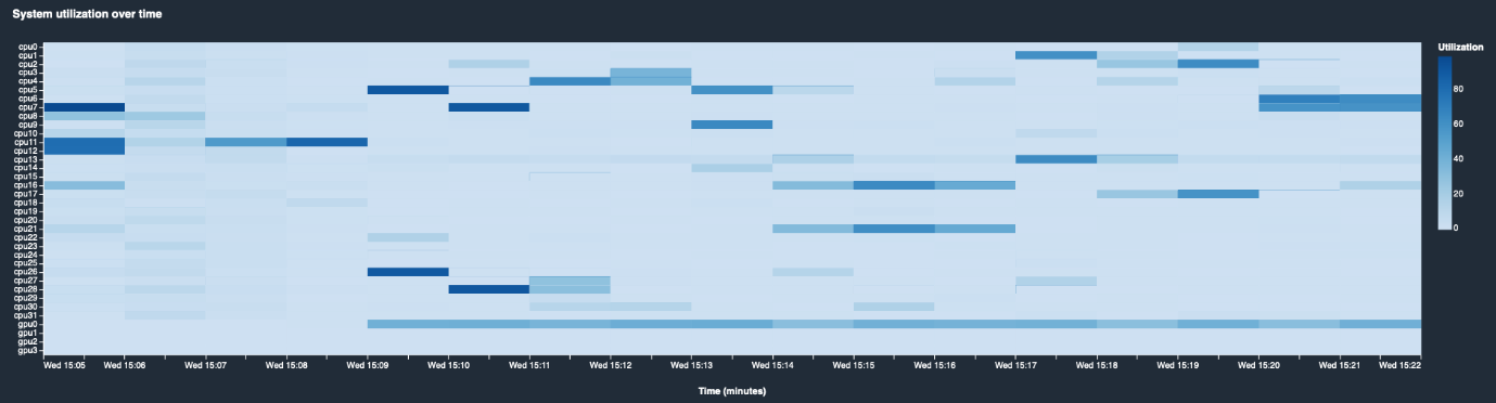
Apparently, this job isn’t going great. GPU utilization and GPU memory utilization are desperately flat at around 10%. I’m definitely not pushing my multi-GPU instance hard enough. Maybe GPUs are not receiving data fast enough because the CPU can’t keep up? Let’s check the system utilization heatmap.

SageMaker screenshot

The CPU is taking a nap here, hardly ever exceeding 20% usage. This instance is definitely not busy enough. Is there anything I could do to fix this?

Switching to the “Overview” panel, I see that some of the built-in profiling rules have been triggered.

SageMaker screenshot

LowGPUUtilization confirms what I saw on the graphs above. BatchSize is very interesting, as it suggests increasing the size of mini-batches sent to the GPUs by the training script running on the CPU. This should definitely help fill GPU memory, put more GPU cores to work, speed up my training job, and improve infrastructure usage.

At this point, I should decide to stop my inefficient training job, and to relaunch it with a larger batch size. Here, I’ll let it run to completion to show you the report generated by the SageMaker Processing job running in parallel of your training job.

Once the training job is complete, I can see its summary in the “Overview” panel.

SageMaker screenshot

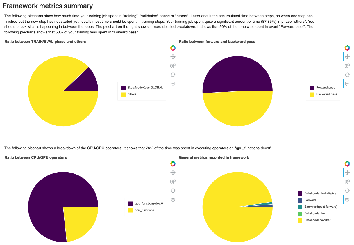
Clicking on the “Download report” button, I get a very detailed report that includes additional metrics, for example the ratio between the different phases of the training job, or the ratio between the forward and backward pass.

SageMaker screenshot

I can also see information on the most time-consuming CPU and GPU operators, which is really important if I wanted to optimize my code. For example, the graph below tells me that the most time-consuming GPU operations in my training job are backward pass convolution operators.

SageMaker screenshot

There’s much more to read in the report (rules summary, training loop analysis, and more). A companion notebook is also available to understand how graphs have been built, and how you can tailor them to your own needs.

Getting Started
We’ve just scratched the surface, and there are many more features in Amazon SageMaker Debugger that make it easy to gather, analyze and visualize model profiling information. You can start using it today in all regions where Amazon SageMaker is available. You won’t be charged for any compute used to run built-in profiling rules.

You’ll find sample notebooks on Github, so give them a try, and let us know what you think. We’re always looking forward to your feedback, either through your usual AWS support contacts, or on the AWS Forum for SageMaker.

– Julien

New – Managed Data Parallelism in Amazon SageMaker Simplifies Training on Large Datasets

Post Syndicated from Julien Simon original https://aws.amazon.com/blogs/aws/managed-data-parallelism-in-amazon-sagemaker-simplifies-training-on-large-datasets/

Today, I’m particularly happy to announce that Amazon SageMaker now supports a new data parallelism library that makes it easier to train models on datasets that may be as large as hundreds or thousands of gigabytes.

As data sets and models grow larger and more sophisticated, machine learning (ML) practitioners working on large distributed training jobs have to face increasingly long training times, even when using powerful instances such as the Amazon Elastic Compute Cloud (EC2) p3 and p4 instances. For example, using a ml.p3dn.24xlarge instance equipped with 8 NVIDIA V100 GPUs, it takes over 6 hours to train advanced object detection models such as Mask RCNN and Faster RCNN on the publicly available COCO dataset. Likewise, training BERT, a state of the art natural language processing model, takes over 100 hours on the same instance. Some of our customers, such as autonomous vehicle companies, routinely deal with even larger training jobs that run for days on large GPU clusters.

As you can imagine, these long training times are a severe bottleneck for ML projects, hurting productivity and slowing down innovation. Customers asked us for help, and we got to work.

Introducing Data Parallelism in Amazon SageMaker
Amazon SageMaker now helps ML teams reduce distributed training time and cost, thanks to the SageMaker Data Parallelism (SDP) library. Available for TensorFlow and PyTorch, SDP implements a more efficient distribution of computation, optimizes network communication, and fully utilizes our fastest p3 and p4 GPU instances.

Up to 90% of GPU resources can now be used for training, not for data transfer. Distributed training jobs can achieve up near-liner scaling efficiency, regardless of the number of GPUs involved. In other words, if a training job runs for 8 hours on a single instance, it will only take approximately 1 hour on 8 instances, with minimal cost increase. SageMaker effectively eliminates any trade-off between training cost and training time, allowing ML teams to get results sooner, iterate faster, and accelerate innovation.

During his keynote at AWS re:Invent 2020, Swami Sivasubramanian demonstrated the fastest training times to date for T5-3B and Mask-RCNN.

  • The T5-3B model has 3 billion parameters, achieves state-of-the-art accuracy on natural language processing benchmarks, and usually takes weeks of effort to train and tune for performance. We trained this model in 6 days on 256 ml.p4d.24xlarge instances.
  • Mask-RCNN continues to be a popular instance segmentation model used by our customers. Last year at re:Invent, we trained Mask-RCNN in 26 minutes on PyTorch, and in 27 minutes on TensorFlow. This year, we recorded the fastest training time to date for Mask-RCNN at 6:12 minutes on TensorFlow, and 6:45 minutes on PyTorch.

Before we explain how Amazon SageMaker is able to achieve such speedups, let’s first explain how data parallelism works, and why it’s hard to scale.

A Primer on Data Parallelism
If you’re training a model on a single GPU, its full internal state is available locally: model parameters, optimizer parameters, gradients (parameter updates computed by backpropagation), and so on. However, things are different when you distribute a training job to a cluster of GPUs.

Using a technique named “data parallelism,” the training set is split in mini-batches that are evenly distributed across GPUs. Thus, each GPU only trains the model on a fraction of the total data set. Obviously, this means that the model state will be slightly different on each GPU, as they will process different batches. In order to ensure training convergence, the model state needs to be regularly updated on all nodes. This can be done synchronously or asynchronously:

  • Synchronous training: all GPUs report their gradient updates either to all other GPUs (many-to-many communication), or to a central parameter server that redistributes them (many-to-one, followed by one-to-many). As all updates are applied simultaneously, the model state is in sync on all GPUs, and the next mini-batch can be processed.
  • Asynchronous training: gradient updates are sent to all other nodes, or to a central server. However, they are applied immediately, meaning that model state will differ from one GPU to the next.

Unfortunately, these techniques don’t scale very well. As the number of GPUs increases, a parameter server will inevitably become a bottleneck. Even without a parameter server, network congestion soon becomes a problem, as n GPUs need to exchange n*(n-1) messages after each iteration, for a total amount of n*(n-1)*model size bytes. For example, ResNet-50 is a popular model used in computer vision applications. With its 26 million parameters, each 32-bit gradient update takes about 100 megabytes. With 8 GPUs, each iteration requires sending and receiving 56 updates, for a total of 5.6 gigabytes. Even with a fast network, this will cause some overhead, and slow down training.

A significant step forward was taken in 2017 thanks to the Horovod project. Horovod implemented an optimized communication algorithm for distributed training named “ring-allreduce,” which was soon integrated with popular deep learning libraries.

In a nutshell, ring-allreduce is a decentralized asynchronous algorithm. There is no parameter server: nodes are organized in a directed cycle graph (to put it simply, a one-way ring). For each iteration, a node receives a gradient update from its predecessor. Once a node has processed its own batch, it applies both updates (its own and the one it received), and sends the results to its neighbor. With n GPUs, each GPU processes 2*(n-1) messages before all GPUs have been updated. Accordingly, the total amount of data exchanged per GPU is 2*(n-1)*model size, which is much better than n*(n-1)*model size.

Still, as datasets keep growing, the network bottleneck issue often rises again. Enter SageMaker and its new AllReduce algorithm.

A New Data Parallelism Algorithm in Amazon SageMaker
With the AllReduce algorithm, GPUs don’t talk to one another any more. Each GPU stores its gradient updates in GPU memory. When a certain threshold is exceeded, these updates are sharded, and sent to parameter servers running on the CPUs of the GPU instances. This removes the need for dedicated parameter servers.

Each CPU is responsible for a subset of the model parameters, and it receives updates coming from all GPUs. For example, with 3 training instances equipped with a single GPU, each GPU in the training cluster would send a third of its gradient updates to each one of the three CPUs.

Illustration

Then, each CPU would apply all the gradient updates that it received, and it would distributes the consolidated result back to all GPUs.

Illustration

Now that we understand how this algorithm works, let’s see how you can use it with your own code, without having to manage any infrastructure.

Training with Data Parallelism in Amazon SageMaker
The SageMaker Data Parallelism API is designed for ease of use, and should provide seamless integration with existing distributed training toolkits. In most cases, all you have to change in your training code is the import statement for Horovod (TensorFlow), or for Distributed Data Parallel (PyTorch).

For PyTorch, this would look like this.

import smdistributed.dataparallel.torch.parallel.distributed as dist
dist.init_process_group()

Then, I need to pin each GPU to a single SDP process.

torch.cuda.set_device(dist.get_local_rank())

Then, I define my model as usual, for example:

class Net(nn.Module):
    def __init__(self):
        super(Net, self).__init__()
        self.conv1 = nn.Conv2d(1, 32, 3, 1)
        self.conv2 = nn.Conv2d(32, 64, 3, 1)
        self.dropout1 = nn.Dropout2d(0.25)
        self.dropout2 = nn.Dropout2d(0.5)
        self.fc1 = nn.Linear(9216, 128)
        self.fc2 = nn.Linear(128, 10)
...

Finally, I instantiate my model, and use it to create a DistributedDataParallel object like so:

import torch
from smdistributed.dataparallel.torch.parallel.distributed import DistributedDataParallel as DDP
device = torch.device("cuda")
model = DDP(Net().to(device))

The rest of the code is vanilla PyTorch, and I can train it using the PyTorch estimator available in the SageMaker SDK. Here, I’m using an ml.p3.16xlarge instance with 8 NVIDIA V100 GPUs.

from sagemaker.pytorch import PyTorch
estimator = PyTorch(
    entry_point='train_pytorch.py',
    role=sagemaker.get_execution_role(),
    framework_version='1.6.0',
    instance_count=1,
    instance_type='ml.p3.16xlarge',
    distribution={'smdistributed':{'dataparallel':{enabled': True}}}
)
estimator.fit()

From then on, SageMaker takes over and provisions all required infrastructure. You can focus on other tasks while your training job runs.

Getting Started
If your training jobs last for hours or days on multiple GPUs, we believe that the SageMaker Data Parallelism library can save you time and money, and help you experiment and innovate quicker. It’s available today at in all regions where SageMaker is available, at no additional cost.

Examples are available to get you started quickly. Give them a try, and let us know what you think. We’re always looking forward to your feedback, either through your usual AWS support contacts, or on the AWS Forum for SageMaker.

– Julien

Amazon SageMaker Continues to Lead the Way in Machine Learning and Announces up to 18% Lower Prices on GPU Instances

Post Syndicated from Julien Simon original https://aws.amazon.com/blogs/aws/amazon-sagemaker-leads-way-in-machine-learning/

Since 2006, Amazon Web Services (AWS) has been helping millions of customers build and manage their IT workloads. From startups to large enterprises to public sector, organizations of all sizes use our cloud computing services to reach unprecedented levels of security, resiliency, and scalability. Every day, they’re able to experiment, innovate, and deploy to production in less time and at lower cost than ever before. Thus, business opportunities can be explored, seized, and turned into industrial-grade products and services.

As Machine Learning (ML) became a growing priority for our customers, they asked us to build an ML service infused with the same agility and robustness. The result was Amazon SageMaker, a fully managed service launched at AWS re:Invent 2017 that provides every developer and data scientist with the ability to build, train, and deploy ML models quickly.

Today, Amazon SageMaker is helping tens of thousands of customers in all industry segments build, train and deploy high quality models in production: financial services (Euler Hermes, Intuit, Slice Labs, Nerdwallet, Root Insurance, Coinbase, NuData Security, Siemens Financial Services), healthcare (GE Healthcare, Cerner, Roche, Celgene, Zocdoc), news and media (Dow Jones, Thomson Reuters, ProQuest, SmartNews, Frame.io, Sportograf), sports (Formula 1, Bundesliga, Olympique de Marseille, NFL, Guiness Six Nations Rugby), retail (Zalando, Zappos, Fabulyst), automotive (Atlas Van Lines, Edmunds, Regit), dating (Tinder), hospitality (Hotels.com, iFood), industry and manufacturing (Veolia, Formosa Plastics), gaming (Voodoo), customer relationship management (Zendesk, Freshworks), energy (Kinect Energy Group, Advanced Microgrid Systems), real estate (Realtor.com), satellite imagery (Digital Globe), human resources (ADP), and many more.

When we asked our customers why they decided to standardize their ML workloads on Amazon SageMaker, the most common answer was: “SageMaker removes the undifferentiated heavy lifting from each step of the ML process.” Zooming in, we identified five areas where SageMaker helps them most.

#1 – Build Secure and Reliable ML Models, Faster
As many ML models are used to serve real-time predictions to business applications and end users, making sure that they stay available and fast is of paramount importance. This is why Amazon SageMaker endpoints have built-in support for load balancing across multiple AWS Availability Zones, as well as built-in Auto Scaling to dynamically adjust the number of provisioned instances according to incoming traffic.

For even more robustness and scalability, Amazon SageMaker relies on production-grade open source model servers such as TensorFlow Serving, the Multi-Model Server, and TorchServe. A collaboration between AWS and Facebook, TorchServe is available as part of the PyTorch project, and makes it easy to deploy trained models at scale without having to write custom code.

In addition to resilient infrastructure and scalable model serving, you can also rely on Amazon SageMaker Model Monitor to catch prediction quality issues that could happen on your endpoints. By saving incoming requests as well as outgoing predictions, and by comparing them to a baseline built from a training set, you can quickly identify and fix problems like missing features or data drift.

Says Aude Giard, Chief Digital Officer at Veolia Water Technologies: “In 8 short weeks, we worked with AWS to develop a prototype that anticipates when to clean or change water filtering membranes in our desalination plants. Using Amazon SageMaker, we built a ML model that learns from previous patterns and predicts the future evolution of fouling indicators. By standardizing our ML workloads on AWS, we were able to reduce costs and prevent downtime while improving the quality of the water produced. These results couldn’t have been realized without the technical experience, trust, and dedication of both teams to achieve one goal: an uninterrupted clean and safe water supply.” You can learn more in this video.

#2 – Build ML Models Your Way
When it comes to building models, Amazon SageMaker gives you plenty of options. You can visit AWS Marketplace, pick an algorithm or a model shared by one of our partners, and deploy it on SageMaker in just a few clicks. Alternatively, you can train a model using one of the built-in algorithms, or your own code written for a popular open source ML framework (TensorFlow, PyTorch, and Apache MXNet), or your own custom code packaged in a Docker container.

You could also rely on Amazon SageMaker AutoPilot, a game-changing AutoML capability. Whether you have little or no ML experience, or you’re a seasoned practitioner who needs to explore hundreds of datasets, SageMaker AutoPilot takes care of everything for you with a single API call. It automatically analyzes your dataset, figures out the type of problem you’re trying to solve, builds several data processing and training pipelines, trains them, and optimizes them for maximum accuracy. In addition, the data processing and training source code is available in auto-generated notebooks that you can review, and run yourself for further experimentation. SageMaker Autopilot also now creates machine learning models up to 40% faster with up to 200% higher accuracy, even with small and imbalanced datasets.

Another popular feature is Automatic Model Tuning. No more manual exploration, no more costly grid search jobs that run for days: using ML optimization, SageMaker quickly converges to high-performance models, saving you time and money, and letting you deploy the best model to production quicker.

NerdWallet relies on data science and ML to connect customers with personalized financial products“, says Ryan Kirkman, Senior Engineering Manager. “We chose to standardize our ML workloads on AWS because it allowed us to quickly modernize our data science engineering practices, removing roadblocks and speeding time-to-delivery. With Amazon SageMaker, our data scientists can spend more time on strategic pursuits and focus more energy where our competitive advantage is—our insights into the problems we’re solving for our users.” You can learn more in this case study.
Says Tejas Bhandarkar, Senior Director of Product, Freshworks Platform: “We chose to standardize our ML workloads on AWS because we could easily build, train, and deploy machine learning models optimized for our customers’ use cases. Thanks to Amazon SageMaker, we have built more than 30,000 models for 11,000 customers while reducing training time for these models from 24 hours to under 33 minutes. With SageMaker Model Monitor, we can keep track of data drifts and retrain models to ensure accuracy. Powered by Amazon SageMaker, Freddy AI Skills is constantly-evolving with smart actions, deep-data insights, and intent-driven conversations.

#3 – Reduce Costs
Building and managing your own ML infrastructure can be costly, and Amazon SageMaker is a great alternative. In fact, we found out that the total cost of ownership (TCO) of Amazon SageMaker over a 3-year horizon is over 54% lower compared to other options, and developers can be up to 10 times more productive. This comes from the fact that Amazon SageMaker manages all the training and prediction infrastructure that ML typically requires, allowing teams to focus exclusively on studying and solving the ML problem at hand.

Furthermore, Amazon SageMaker includes many features that help training jobs run as fast and as cost-effectively as possible: optimized versions of the most popular machine learning libraries, a wide range of CPU and GPU instances with up to 100GB networking, and of course Managed Spot Training which lets you save up to 90% on your training jobs. Last but not least, Amazon SageMaker Debugger automatically identifies complex issues developing in ML training jobs. Unproductive jobs are terminated early, and you can use model information captured during training to pinpoint the root cause.

Amazon SageMaker also helps you slash your prediction costs. Thanks to Multi-Model Endpoints, you can deploy several models on a single prediction endpoint, avoiding the extra work and cost associated with running many low-traffic endpoints. For models that require some hardware acceleration without the need for a full-fledged GPU, Amazon Elastic Inference lets you save up to 90% on your prediction costs. At the other end of the spectrum, large-scale prediction workloads can rely on AWS Inferentia, a custom chip designed by AWS, for up to 30% higher throughput and up to 45% lower cost per inference compared to GPU instances.

Lyft, one of the largest transportation networks in the United States and Canada, launched its Level 5 autonomous vehicle division in 2017 to develop a self-driving system to help millions of riders. Lyft Level 5 aggregates over 10 terabytes of data each day to train ML models for their fleet of autonomous vehicles. Managing ML workloads on their own was becoming time-consuming and expensive. Says Alex Bain, Lead for ML Systems at Lyft Level 5: “Using Amazon SageMaker distributed training, we reduced our model training time from days to couple of hours. By running our ML workloads on AWS, we streamlined our development cycles and reduced costs, ultimately accelerating our mission to deliver self-driving capabilities to our customers.

#4 – Build Secure and Compliant ML Systems
Security is always priority #1 at AWS. It’s particularly important to customers operating in regulated industries such as financial services or healthcare, as they must implement their solutions with the highest level of security and compliance. For this purpose, Amazon SageMaker implements many security features, making it compliant with the following global standards: SOC 1/2/3, PCI, ISO, FedRAMP, DoD CC SRG, IRAP, MTCS, C5, K-ISMS, ENS High, OSPAR, and HITRUST CSF. It’s also HIPAA BAA eligible.

Says Ashok Srivastava, Chief Data Officer, Intuit: “With Amazon SageMaker, we can accelerate our Artificial Intelligence initiatives at scale by building and deploying our algorithms on the platform. We will create novel large-scale machine learning and AI algorithms and deploy them on this platform to solve complex problems that can power prosperity for our customers.”

#5 – Annotate Data and Keep Humans in the Loop
As ML practitioners know, turning data into a dataset requires a lot of time and effort. To help you reduce both, Amazon SageMaker Ground Truth is a fully managed data labeling service that makes it easy to annotate and build highly accurate training datasets at any scale (text, image, video, and 3D point cloud datasets).

Says Magnus Soderberg, Director, Pathology Research, AstraZeneca: “AstraZeneca has been experimenting with machine learning across all stages of research and development, and most recently in pathology to speed up the review of tissue samples. The machine learning models first learn from a large, representative data set. Labeling the data is another time-consuming step, especially in this case, where it can take many thousands of tissue sample images to train an accurate model. AstraZeneca uses Amazon SageMaker Ground Truth, a machine learning-powered, human-in-the-loop data labeling and annotation service to automate some of the most tedious portions of this work, resulting in reduction of time spent cataloging samples by at least 50%.

Amazon SageMaker is Evaluated
The hundreds of new features added to Amazon SageMaker since launch are testimony to our relentless innovation on behalf of customers. In fact, the service was highlighted in February 2020 as the overall leader in Gartner’s Cloud AI Developer Services Magic Quadrant. Gartner subscribers can click here to learn more about why we have an overall score of 84/100 in their “Solution Scorecard for Amazon SageMaker, July 2020”, the highest rating among our peer group. According to Gartner, we met 87% of required criteria, 73% of preferred, and 85% of optional.

Announcing a Price Reduction on GPU Instances

To thank our customers for their trust and to show our continued commitment to make Amazon SageMaker the best and most cost-effective ML service, I’m extremely happy to announce a significant price reduction on all ml.p2 and ml.p3 GPU instances. It will apply starting October 1st for all SageMaker components and across the following regions: US East (N. Virginia), US East (Ohio), US West (Oregon), EU (Ireland), EU (Frankfurt), EU (London), Canada (Central), Asia Pacific (Singapore), Asia Pacific (Sydney), Asia Pacific (Seoul), Asia Pacific (Tokyo), Asia Pacific (Mumbai), and AWS GovCloud (US-Gov-West).

Instance Name Price Reduction
ml.p2.xlarge -11%
ml.p2.8xlarge -14%
ml.p2.16xlarge -18%
ml.p3.2xlarge -11%
ml.p3.8xlarge -14%
ml.p3.16xlarge -18%
ml.p3dn.24xlarge -18%

Getting Started with Amazon SageMaker
As you can see, there are a lot of exciting features in Amazon SageMaker, and I encourage you to try them out! Amazon SageMaker is available worldwide, so chances are you can easily get to work on your own datasets. The service is part of the AWS Free Tier, letting new users work with it for free for hundreds of hours during the first two months.

If you’d like to kick the tires, this tutorial will get you started in minutes. You’ll learn how to use SageMaker Studio to build, train, and deploy a classification model based on the XGBoost algorithm.

Last but not least, I just published a book named “Learn Amazon SageMaker“, a 500-page detailed tour of all SageMaker features, illustrated by more than 60 original Jupyter notebooks. It should help you get up to speed in no time.

As always, we’re looking forward to your feedback. Please share it with your usual AWS support contacts, or on the AWS Forum for SageMaker.

– Julien