Post Syndicated from Marek Majkowski original https://blog.cloudflare.com/quic-restarts-slow-problems-udpgrm-to-the-rescue/
At Cloudflare, we do everything we can to avoid interruption to our services. We frequently deploy new versions of the code that delivers the services, so we need to be able to restart the server processes to upgrade them without missing a beat. In particular, performing graceful restarts (also known as “zero downtime”) for UDP servers has proven to be surprisingly difficult.
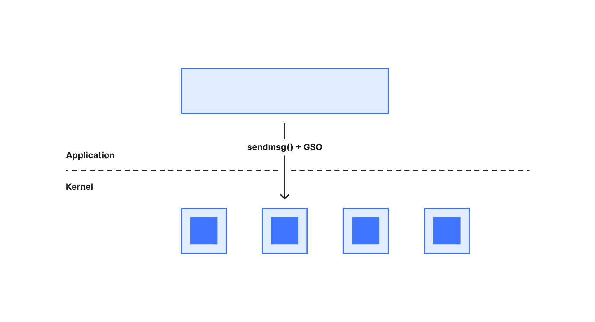
We’ve previously written about graceful restarts in the context of TCP, which is much easier to handle. We didn’t have a strong reason to deal with UDP until recently — when protocols like HTTP3/QUIC became critical. This blog post introduces udpgrm, a lightweight daemon that helps us to upgrade UDP servers without dropping a single packet.
Here’s the udpgrm GitHub repo.
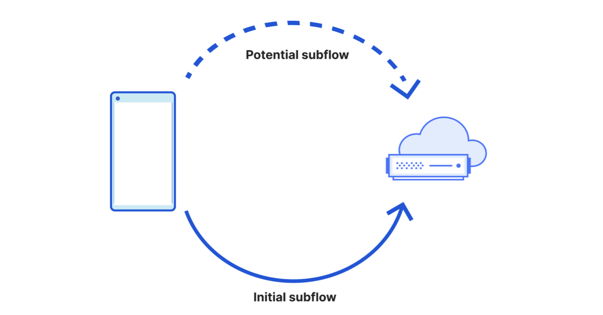
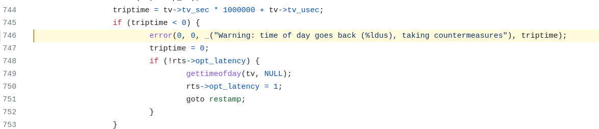
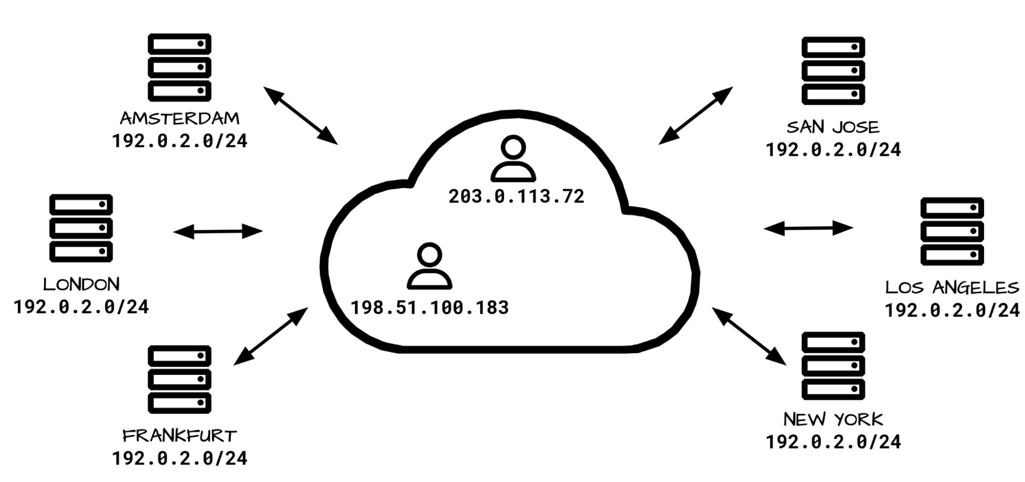
In the early days of the Internet, UDP was used for stateless request/response communication with protocols like DNS or NTP. Restarts of a server process are not a problem in that context, because it does not have to retain state across multiple requests. However, modern protocols like QUIC, WireGuard, and SIP, as well as online games, use stateful flows. So what happens to the state associated with a flow when a server process is restarted? Typically, old connections are just dropped during a server restart. Migrating the flow state from the old instance to the new instance is possible, but it is complicated and notoriously hard to get right.
The same problem occurs for TCP connections, but there a common approach is to keep the old instance of the server process running alongside the new instance for a while, routing new connections to the new instance while letting existing ones drain on the old. Once all connections finish or a timeout is reached, the old instance can be safely shut down. The same approach works for UDP, but it requires more involvement from the server process than for TCP.
In the past, we described the established-over-unconnected method. It offers one way to implement flow handoff, but it comes with significant drawbacks: it’s prone to race conditions in protocols with multi-packet handshakes, and it suffers from a scalability issue. Specifically, the kernel hash table used for dispatching packets is keyed only by the local IP:port tuple, which can lead to bucket overfill when dealing with many inbound UDP sockets.
Now we have found a better method, leveraging Linux’s SO_REUSEPORT API. By placing both old and new sockets into the same REUSEPORT group and using an eBPF program for flow tracking, we can route packets to the correct instance and preserve flow stickiness. This is how udpgrm works.
Before diving deeper, let’s quickly review the basics. Linux provides the SO_REUSEPORT socket option, typically set after socket() but before bind(). Please note that this has a separate purpose from the better known SO_REUSEADDR socket option.
SO_REUSEPORT allows multiple sockets to bind to the same IP:port tuple. This feature is primarily used for load balancing, letting servers spread traffic efficiently across multiple CPU cores. You can think of it as a way for an IP:port to be associated with multiple packet queues. In the kernel, sockets sharing an IP:port this way are organized into a reuseport group — a term we’ll refer to frequently throughout this post.
┌───────────────────────────────────────────┐
│ reuseport group 192.0.2.0:443             │
│ ┌───────────┐ ┌───────────┐ ┌───────────┐ │
│ │ socket #1 │ │ socket #2 │ │ socket #3 │ │
│ └───────────┘ └───────────┘ └───────────┘ │
└───────────────────────────────────────────┘
Linux supports several methods for distributing inbound packets across a reuseport group. By default, the kernel uses a hash of the packet’s 4-tuple to select a target socket. Another method is SO_INCOMING_CPU, which, when enabled, tries to steer packets to sockets running on the same CPU that received the packet. This approach works but has limited flexibility.
To provide more control, Linux introduced the SO_ATTACH_REUSEPORT_CBPF option, allowing server processes to attach a classic BPF (cBPF) program to make socket selection decisions. This was later extended with SO_ATTACH_REUSEPORT_EBPF, enabling the use of modern eBPF programs. With eBPF, developers can implement arbitrary custom logic. A boilerplate program would look like this:
SEC("sk_reuseport")
int udpgrm_reuseport_prog(struct sk_reuseport_md *md)
{
    uint64_t socket_identifier = xxxx;
    bpf_sk_select_reuseport(md, &sockhash, &socket_identifier, 0);
    return SK_PASS;
}
To select a specific socket, the eBPF program calls bpf_sk_select_reuseport, using a reference to a map with sockets (SOCKHASH, SOCKMAP, or the older, mostly obsolete SOCKARRAY), along with a key or index. For example, a declaration of a SOCKHASH might look like this:
struct {
	__uint(type, BPF_MAP_TYPE_SOCKHASH);
	__uint(max_entries, MAX_SOCKETS);
	__uint(key_size, sizeof(uint64_t));
	__uint(value_size, sizeof(uint64_t));
} sockhash SEC(".maps");
This SOCKHASH is a hash map that holds references to sockets, even though the value size looks like a scalar 8-byte value. In our case it’s indexed by an uint64_t key. This is pretty neat, as it allows for a simple number-to-socket mapping!
However, there’s a catch: the SOCKHASH must be populated and maintained from user space (or a separate control plane), outside the eBPF program itself. Keeping this socket map accurate and in sync with the server process state is surprisingly difficult to get right — especially under dynamic conditions like restarts, crashes, or scaling events. The point of udpgrm is to take care of this stuff, so that server processes don’t have to.
Let’s look at how graceful restarts for UDP flows are achieved in udpgrm. To reason about this setup, we’ll need a bit of terminology: A socket generation is a set of sockets within a reuseport group that belong to the same logical application instance:
┌───────────────────────────────────────────────────┐
│ reuseport group 192.0.2.0:443                     │
│  ┌─────────────────────────────────────────────┐  │
│  │ socket generation 0                         │  │
│  │  ┌───────────┐ ┌───────────┐ ┌───────────┐  │  │
│  │  │ socket #1 │ │ socket #2 │ │ socket #3 │  │  │
│  │  └───────────┘ └───────────┘ └───────────┘  │  │
│  └─────────────────────────────────────────────┘  │
│  ┌─────────────────────────────────────────────┐  │
│  │ socket generation 1                         │  │
│  │  ┌───────────┐ ┌───────────┐ ┌───────────┐  │  │
│  │  │ socket #4 │ │ socket #5 │ │ socket #6 │  │  │
│  │  └───────────┘ └───────────┘ └───────────┘  │  │
│  └─────────────────────────────────────────────┘  │
└───────────────────────────────────────────────────┘
When a server process needs to be restarted, the new version creates a new socket generation for its sockets. The old version keeps running alongside the new one, using sockets from the previous socket generation.
Reuseport eBPF routing boils down to two problems:
-
For new flows, we should choose a socket from the socket generation that belongs to the active server instance.
-
For already established flows, we should choose the appropriate socket — possibly from an older socket generation — to keep the flows sticky. The flows will eventually drain away, allowing the old server instance to shut down.
Easy, right?
Of course not! The devil is in the details. Let’s take it one step at a time.
Routing new flows is relatively easy. udpgrm simply maintains a reference to the socket generation that should handle new connections. We call this reference the working generation. Whenever a new flow arrives, the eBPF program consults the working generation pointer and selects a socket from that generation.
┌──────────────────────────────────────────────┐
│ reuseport group 192.0.2.0:443 │
│ ... │
│ Working generation ────┐ │
│ V │
│ ┌───────────────────────────────┐ │
│ │ socket generation 1 │ │
│ │ ┌───────────┐ ┌──────────┐ │ │
│ │ │ socket #4 │ │ ... │ │ │
│ │ └───────────┘ └──────────┘ │ │
│ └───────────────────────────────┘ │
│ ... │
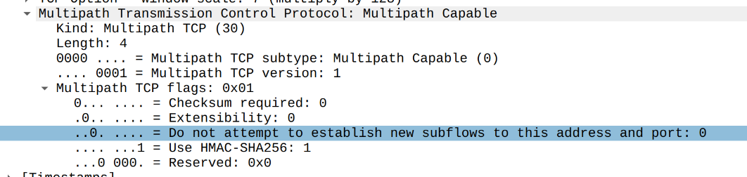
└──────────────────────────────────────────────┘For this to work, we first need to be able to differentiate packets belonging to new connections from packets belonging to old connections. This is very tricky and highly dependent on the specific UDP protocol. For example, QUIC has an initial packet concept, similar to a TCP SYN, but other protocols might not.
There needs to be some flexibility in this and udpgrm makes this configurable. Each reuseport group sets a specific flow dissector.
Flow dissector has two tasks:
-
It distinguishes new packets from packets belonging to old, already established flows.
-
For recognized flows, it tells udpgrm which specific socket the flow belongs to.
These concepts are closely related and depend on the specific server. Different UDP protocols define flows differently. For example, a naive UDP server might use a typical 5-tuple to define flows, while QUIC uses a “connection ID” field in the QUIC packet header to survive NAT rebinding.
udpgrm supports three flow dissectors out of the box and is highly configurable to support any UDP protocol. More on this later.
Now that we covered the theory, we’re ready for the business: please welcome udpgrm — UDP Graceful Restart Marshal! udpgrm is a stateful daemon that handles all the complexities of the graceful restart process for UDP. It installs the appropriate eBPF REUSEPORT program, maintains flow state, communicates with the server process during restarts, and reports useful metrics for easier debugging.
We can describe udpgrm from two perspectives: for administrators and for programmers.
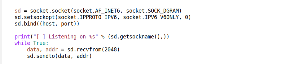
udpgrm is a stateful daemon, to run it:
$ sudo udpgrm --daemon
[ ] Loading BPF code
[ ] Pinning bpf programs to /sys/fs/bpf/udpgrm
[*] Tailing message ring buffer  map_id 936146
This sets up the basic functionality, prints rudimentary logs, and should be deployed as a dedicated systemd service — loaded after networking. However, this is not enough to fully use udpgrm. udpgrm needs to hook into getsockopt, setsockopt, bind, and sendmsg syscalls, which are scoped to a cgroup. To install the udpgrm hooks, you can install it like this:
$ sudo udpgrm --install=/sys/fs/cgroup/system.sliceBut a more common pattern is to install it within the current cgroup:
$ sudo udpgrm --install --selfBetter yet, use it as part of the systemd “service” config:
[Service]
...
ExecStartPre=/usr/local/bin/udpgrm --install --self
Once udpgrm is running, the administrator can use the CLI to list reuseport groups, sockets, and metrics, like this:
$ sudo udpgrm list
[ ] Retrievieng BPF progs from /sys/fs/bpf/udpgrm
192.0.2.0:4433
	netns 0x1  dissector bespoke  digest 0xdead
	socket generations:
		gen  3  0x17a0da  <=  app 0  gen 3
	metrics:
		rx_processed_total 13777528077
...
Now, with both the udpgrm daemon running, and cgroup hooks set up, we can focus on the server part.
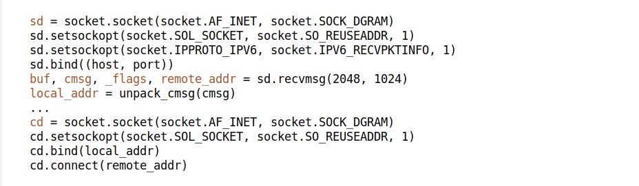
We expect the server to create the appropriate UDP sockets by itself. We depend on SO_REUSEPORT, so that each server instance can have a dedicated socket or a set of sockets:
sd = socket.socket(AF_INET, SOCK_DGRAM, 0)
sd.setsockopt(SOL_SOCKET, SO_REUSEPORT, 1)
sd.bind(("192.0.2.1", 5201))
With a socket descriptor handy, we can pursue the udpgrm magic dance. The server communicates with the udpgrm daemon using setsockopt calls. Behind the scenes, udpgrm provides eBPF setsockopt and getsockopt hooks and hijacks specific calls. It’s not easy to set up on the kernel side, but when it works, it’s truly awesome. A typical socket setup looks like this:
try:
    work_gen = sd.getsockopt(IPPROTO_UDP, UDP_GRM_WORKING_GEN)
except OSError:
    raise OSError('Is udpgrm daemon loaded? Try "udpgrm --self --install"')

sd.setsockopt(IPPROTO_UDP, UDP_GRM_SOCKET_GEN, work_gen + 1)
for i in range(10):
    v = sd.getsockopt(IPPROTO_UDP, UDP_GRM_SOCKET_GEN, 8);
    sk_gen, sk_idx = struct.unpack('II', v)
    if sk_idx != 0xffffffff:
        break
    time.sleep(0.01 * (2 ** i))
else:
    raise OSError("Communicating with udpgrm daemon failed.")

sd.setsockopt(IPPROTO_UDP, UDP_GRM_WORKING_GEN, work_gen + 1)
You can see three blocks here:
-
First, we retrieve the working generation number and, by doing so, check for udpgrm presence. Typically, udpgrm absence is fine for non-production workloads.
-
Then we register the socket to an arbitrary socket generation. We choose
work_gen + 1as the value and verify that the registration went through correctly. -
Finally, we bump the working generation pointer.
That’s it! Hopefully, the API presented here is clear and reasonable. Under the hood, the udpgrm daemon installs the REUSEPORT eBPF program, sets up internal data structures, collects metrics, and manages the sockets in a SOCKHASH.
In practice, we often need sockets bound to low ports like :443, which requires elevated privileges like CAP_NET_BIND_SERVICE. It’s usually better to configure listening sockets outside the server itself. A typical pattern is to pass the listening sockets using socket activation.
Sadly, systemd cannot create a new set of UDP SO_REUSEPORT sockets for each server instance. To overcome this limitation, udpgrm provides a script called udpgrm_activate.py, which can be used like this:
[Service]
Type=notify                 # Enable access to fd store
NotifyAccess=all            # Allow access to fd store from ExecStartPre
FileDescriptorStoreMax=128  # Limit of stored sockets must be set

ExecStartPre=/usr/local/bin/udpgrm_activate.py test-port 0.0.0.0:5201
Here, udpgrm_activate.py binds to 0.0.0.0:5201 and stores the created socket in the systemd FD store under the name test-port. The server echoserver.py will inherit this socket and receive the appropriate FD_LISTEN environment variables, following the typical systemd socket activation pattern.
Systemd typically can’t handle more than one server instance running at the same time. It prefers to kill the old instance quickly. It supports the “at most one” server instance model, not the “at least one” model that we want. To work around this, udpgrm provides a decoy script that will exit when systemd asks it to, while the actual old instance of the server can stay active in the background.
[Service]
...
ExecStart=/usr/local/bin/mmdecoy examples/echoserver.py

Restart=always             # if pid dies, restart it.
KillMode=process           # Kill only decoy, keep children after stop.
KillSignal=SIGTERM         # Make signals explicit
At this point, we showed a full template for a udpgrm enabled server that contains all three elements: udpgrm --install --self for cgroup hooks, udpgrm_activate.py for socket creation, and mmdecoy for fooling systemd service lifetime checks.
[Service]
Type=notify                 # Enable access to fd store
NotifyAccess=all            # Allow access to fd store from ExecStartPre
FileDescriptorStoreMax=128  # Limit of stored sockets must be set

ExecStartPre=/usr/local/bin/udpgrm --install --self
ExecStartPre=/usr/local/bin/udpgrm_activate.py --no-register test-port 0.0.0.0:5201
ExecStart=/usr/local/bin/mmdecoy PWD/examples/echoserver.py

Restart=always             # if pid dies, restart it.
KillMode=process           # Kill only decoy, keep children after stop.
KillSignal=SIGTERM # Make signals explicitWe’ve discussed the udpgrm daemon, the udpgrm setsockopt API, and systemd integration, but we haven’t yet covered the details of routing logic for old flows. To handle arbitrary protocols, udpgrm supports three dissector modes out of the box:
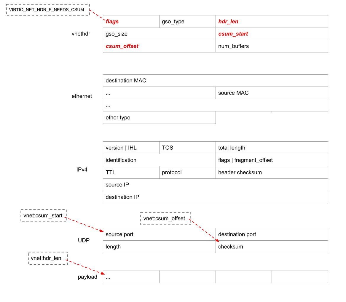
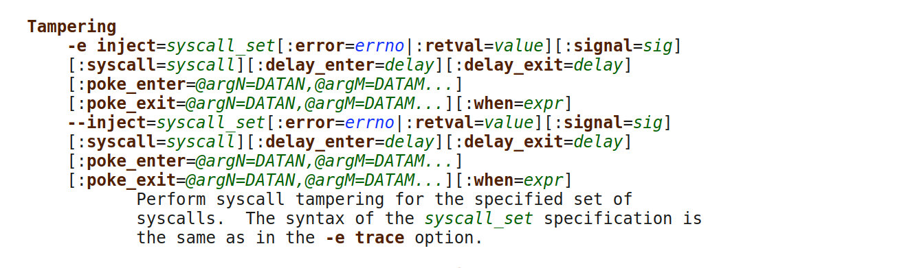
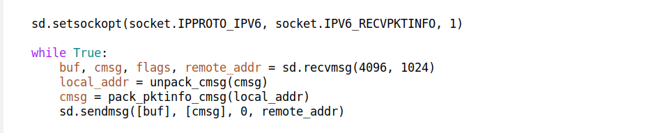
DISSECTOR_FLOW: udpgrm maintains a flow table indexed by a flow hash computed from a typical 4-tuple. It stores a target socket identifier for each flow. The flow table size is fixed, so there is a limit to the number of concurrent flows supported by this mode. To mark a flow as “assured,” udpgrm hooks into the sendmsg syscall and saves the flow in the table only when a message is sent.
DISSECTOR_CBPF: A cookie-based model where the target socket identifier — called a udpgrm cookie — is encoded in each incoming UDP packet. For example, in QUIC, this identifier can be stored as part of the connection ID. The dissection logic is expressed as cBPF code. This model does not require a flow table in udpgrm but is harder to integrate because it needs protocol and server support.
DISSECTOR_NOOP: A no-op mode with no state tracking at all. It is useful for traditional UDP services like DNS, where we want to avoid losing even a single packet during an upgrade.
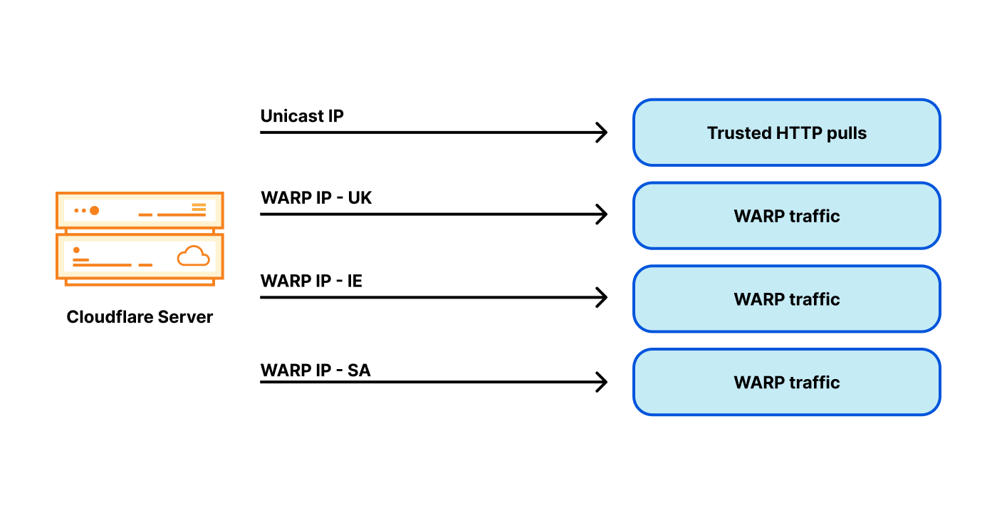
Finally, udpgrm provides a template for a more advanced dissector called DISSECTOR_BESPOKE. Currently, it includes a QUIC dissector that can decode the QUIC TLS SNI and direct specific TLS hostnames to specific socket generations.
For more details, please consult the udpgrm README. In short: the FLOW dissector is the simplest one, useful for old protocols. CBPF dissector is good for experimentation when the protocol allows storing a custom connection id (cookie) — we used it to develop our own QUIC Connection ID schema (also named DCID) — but it’s slow, because it interprets cBPF inside eBPF (yes really!). NOOP is useful, but only for very specific niche servers. The real magic is in the BESPOKE type, where users can create arbitrary, fast, and powerful dissector logic.
The adoption of QUIC and other UDP-based protocols means that gracefully restarting UDP servers is becoming an increasingly important problem. To our knowledge, a reusable, configurable and easy to use solution didn’t exist yet. The udpgrm project brings together several novel ideas: a clean API using setsockopt(), careful socket-stealing logic hidden under the hood, powerful and expressive configurable dissectors, and well-thought-out integration with systemd.
While udpgrm is intended to be easy to use, it hides a lot of complexity and solves a genuinely hard problem. The core issue is that the Linux Sockets API has not kept up with the modern needs of UDP.
Ideally, most of this should really be a feature of systemd. That includes supporting the “at least one” server instance mode, UDP SO_REUSEPORT socket creation, installing a REUSEPORT_EBPF program, and managing the “working generation” pointer. We hope that udpgrm helps create the space and vocabulary for these long-term improvements.