All posts by Navnit Shukla

Reference guide for building a self-service analytics solution with Amazon SageMaker

Post Syndicated from Navnit Shukla original https://aws.amazon.com/blogs/big-data/reference-guide-for-building-a-self-service-analytics-solution-with-amazon-sagemaker/

Organizations today face a critical challenge with fragmented data scattered across multiple silos, including data lakes, warehouses, SaaS applications, and legacy systems. This disconnect prevents businesses from gaining a holistic view of their customers, optimizing operations, and making real-time data-driven decisions. To stay competitive, companies are turning to self-service analytics, enabling both business and technical users to quickly access, explore, and analyze data without dependency on IT teams.

However, implementing self-service analytics comes with significant challenges. Organizations must address integrating data from diverse sources for seamless access, creating business and technical catalogs to improve data discoverability, enabling data lineage and quality to build trust and reliability, implementing fine-grained access controls to ensure security and compliance, providing role-specific tools for data engineers, analysts, and artificial intelligence (AI)/machine learning (ML) teams, and establishing governance frameworks to enforce policies and regulatory requirements.

In this post, we show how to use Amazon SageMaker Catalog to publish data from multiple sources, including Amazon S3, Amazon Redshift, and Snowflake. This approach enables self-service access while ensuring robust data governance and metadata management. By centralizing metadata, users can improve data discoverability, lineage tracking, and compliance while empowering analysts, data engineers, and data scientists to derive AI-driven insights efficiently and securely. We use a sample retail use case to demonstrate the solution, making it easier to understand how these capabilities can be applied to real-world scenarios.

Amazon SageMaker: Enabling self-service analytics

Amazon SageMaker brings together AWS AI/ML and analytics capabilities, delivering an integrated experience for analytics and AI with unified data access, enabling teams to:

  • Discover and access data stored across Amazon S3, Amazon Redshift, and other third-party sources through the Lakehouse architecture.
  • Perform complete AI and analytics workflows using familiar AWS services for data analysis, processing, model training, and generative AI app development.
  • Use Amazon Q Developer, an advanced generative AI assistant to accelerate software development.
  • Ensure enterprise-grade security with built-in governance, fine-grained access controls, and secure artifact sharing with Amazon SageMaker Catalog.
  • Collaborate in shared projects, allowing teams to work together efficiently while maintaining compliance and governance.

Retail use case overview

In our example, a retail organization operates across multiple business units, each storing data in different platforms, creating challenges in data access, consistency, and governance.


Figure 1: High-level architecture of our retail use case showing data flow across multiple systems

Our retail organization faces data fragmentation across its business units:

  • The Wholesale Sales business unit stores its data in Amazon S3.
  • The Store Sales business unit maintains its transactional data in Amazon Redshift.
  • Online Sales Data is stored in Snowflake.

These disparate data sources result in data silos, inconsistent schemas, duplication, and missing values, making it difficult for analysts and AI-driven solutions to derive meaningful insights.

Data model

The following Entity-Relationship (ER) Diagram represents the dataset structure and relationships between different entities in Wholesale, Retail, and Online Sales Data:


Figure 2: Entity-Relationship Diagram showing the relationships between different data entities

Key entities in our data model

Our sample dataset models a multi-channel retail business with interconnected entities representing products, sales channels, customers, and locations.

  1. PRODUCTS is a central entity that links to WHOLESALE_SALES, RETAIL_SALES, and ONLINE_SALES, representing product transactions across different sales channels.
  2. WHOLESALE_SALES records bulk transactions where WAREHOUSES distribute products to retailers. Each sale is associated with a PRODUCT and a WAREHOUSE.
  3. RETAIL_SALES captures individual purchases made in physical STORES. Each transaction involves a PRODUCT and a STORE, along with details like quantity sold, discount applied, and revenue.
  4. ONLINE_SALES tracks e-commerce transactions where customers buy products online. Each record links to a CUSTOMER and a PRODUCT, along with details like quantity, price, and shipping information.
  5. CUSTOMERS represent buyers in the system and are linked to ONLINE_SALES (for purchasing) and CUSTOMER_REVIEWS (for leaving product reviews).
  6. CUSTOMER_REVIEWS stores feedback provided by customers for products they purchased online. Each review is linked to an ONLINE_SALES order, a CUSTOMER, and a PRODUCT.
  7. STORES represent physical retail locations where products are sold. They are associated with RETAIL_SALES, indicating that products are purchased in-store.
  8. WAREHOUSES are responsible for stocking and distributing products through WHOLESALE_SALES transactions. They manage stock levels and facilitate bulk sales to retailers.

Data distribution across systems

To simulate a real-world enterprise scenario, our data is distributed across multiple systems and AWS accounts as follows:

Accounts Location Tables
Wholesale Amazon S3 WHOLESALE_SALES, PRODUCT, WAREHOUSE
Store Amazon Redshift RETAIL_SALES, STORE, PRODUCT
Online Sales Snowflake ONLINE_SALES, CUSTOMER, CUSTOMER_REVIEWS, PRODUCT

Assumptions

We are making the following assumptions for this implementation.

Building the SageMaker Catalog

In this section, we walk through the process of creating the SageMaker Catalog from multiple sources using Amazon SageMaker Unified Studio.

Step 1: Setting up your SageMaker Unified Studio environment

Before we begin building our data catalog, we cover some terminology for SageMaker Unified Studio.

Domain: A domain in Amazon SageMaker Unified Studio is a logical boundary that serves as the primary container for all your data assets, users, and resources, allowing efficient data organization and management.
Domain Units: Domain units are subcomponents within a domain that help organize related projects and resources together, enabling hierarchical structuring of your data management activities.
Blueprint: A blueprint in Amazon SageMaker Unified Studio is a template that defines standardized configurations for projects, including what resources are provisioned, and what tools, and parameters are applied.
Project Profile: A project profile is a collection of blueprints which are configurations used to create projects. A project profile can define if a particular blueprint is enabled during the creation of the project, or available later for the project users to enable on-demand.
Project: A project in Amazon SageMaker Unified Studio is a boundary within a domain where users can collaborate with others to work on a business use case. In projects, users can create and share data and resources.

Now, we can set up our Amazon SageMaker Unified Studio environment.

Create a SageMaker domain

  1. Open the Amazon SageMaker management console in the Centralized Processing account and use the region selector in the top navigation bar to choose the appropriate AWS Region.
  2. Choose Create a Unified Studio domain.
  3. Choose Quick setup as explained in Create an Amazon SageMaker Unified Studio domain – quick setup.
  4. For Create IAM Identity Center User, search for SSO users through email addresses.
    If there is no Amazon Identity Access Manager (IAM) Identity Center instance, a prompt appears to enter your name after your email address. This creates a new local IAM Identity Center instance.
  5. Choose Create domain.

Log in to SageMaker Unified Studio

Now that we have created a new SageMaker Unified Studio domain, complete the following steps to visit the Amazon SageMaker Unified Studio.

  1. On the SageMaker platform console, open the details page of your domain.
  2. Choose the link for Amazon SageMaker Unified Studio URL.
  3. Log in with your SSO credentials.

Now you signed in to the SageMaker Unified Studio.

Create a project

The next step is to create a project. Complete the following steps:

  1. On the SageMaker Unified Studio, choose Select a project on the top menu, and choose Create project.
  2. For Project name, enter a name (such as AnyCompanyDataPlatform).
  3. For Project profile, choose All capabilities.
  4. Choose Continue.
  5. Review the input and choose Create project. This project serves as a collaborative workspace for our data integration efforts.

Wait for the project to be created. Project creation can take about five minutes. Then The SageMaker Unified Studio console goes to the project’s home page.

Step 2: Connecting to data sources

Now, we connect to our various data sources to bring them into our data catalog.

Importing existing AWS Glue Data Catalog (Wholesale Sales Data)

We first import the wholesale sales data from Amazon S3 in the Wholesale account into Amazon SageMaker Unified Studio.

Set up cross-account access

  1. Log in to Centralized Processing account and create a Glue Crawler role named glue-cross-s3-access with the AWSGlueServiceRole and cross account S3 access policy for Wholesale account.
    Sample cross account S3 access policy:

    { "Version": "2012-10-17", "Statement": [ { "Effect": "Allow", "Action": [ "s3:GetObject" ], "Resource": [ "arn:aws:s3:::<wholesale-account-bucket>/*" ] } ]}

  2. Log in to the Wholesale account and create an S3 bucket policy that grants access to S3 data files for the previously created glue-cross-s3-access role of the Centralized Processing account.
  3. Log in to the Centralized Processing account and create a database named anycompanydatacatlog from the AWS Glue.
  4. Grant permissions to the glue-cross-s3-access role for the anycompanydatacatalog database in AWS Lake Formation.
  5. Run the Glue Crawler using the glue-cross-s3-access role to scan the S3 bucket in the Wholesale account. For more information, refer to the tutorial explaining how to catalog S3 data using the Glue crawler.
  6. Verify the anycompanydatacatlog database and its corresponding tables.

Configure the Glue data catalog assets

  1. Download the provided scripts from the Bring Your Own Glue Data Catalog Assets repository.
  2. Copy the Amazon SageMaker Unified Studio project role ARN from project overview section.
  3. Add the same Amazon SageMaker Unified Studio project role as LakeFormation Data Lake Administrator.

Import the assets into Amazon SageMaker Unified Studio

  1. Open AWS CloudShell in the Centralized Processing account console.
  2. Upload the previously downloaded bring_your_own_gdc_assets.py file to AWS CloudShell.
  3. Run the import script in AWS CloudShell with following parameters.
    1. project-role-arn: Enter the project role ARN of SageMaker Unified Studio.
    2. database-name: Enter the database name of Glue Catalog (such as anycompanydatacatalog).
    3. region: Enter the region of SageMaker Unified Studio (such as us-east-1).
    python3 bring_your_own_gdc_assets.py \
    --project-role-arn <Project role ARN> \
    --database-name <Glue Database name to import> \
    --region <region-code>

Verify the imported wholesale sales data

  1. In the Centralized Processing account, go to the SageMaker Unified Studio console, choose your project.
  2. Choose Data in the navigation pane.
  3. Confirm that the wholesale_db database and its tables (WHOLESALE_SALES, PRODUCT, WAREHOUSE) are now available under anycompanydatacatalog.

Connecting to Amazon Redshift (Stores sales data)

In this step, we bring stores sales data from Amazon Redshift in the Store account into Amazon SageMaker Unified Studio.

Set up cross-account access

  1. Login to the Store account, create a virtual private cloud (VPC) peering connection between the Store account and the Centralized Processing account, which hosts the Amazon SageMaker Unified Studio, and configure route tables following the documentation.
  2. Update your Redshift VPC security group’s rule to include the Centralized Processing account’s IPv4 CIDR range, enabling network connectivity and allowing incoming requests from the Centralized Processing account to access the Store account resources.

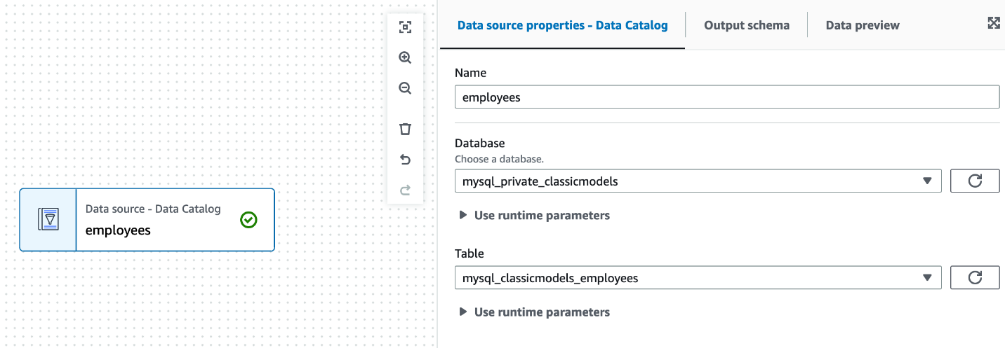
Create a federated connection for Amazon Redshift

  1. In the Centralized Processing account, go to the SageMaker Unified Studio console, choose your project.
  2. Choose Data in the navigation pane.
  3. In the data explorer, choose the plus sign to add a data source.
  4. Under add a data source, choose Add connection, then choose Amazon Redshift.
  5. Enter the following parameters in the connection details, and choose Add data.
    1. Name: Enter the connection name (such as anycompanyredshift).
    2. Host: Enter the Amazon Redshift cluster endpoint.
    3. Port: Enter the port number (Amazon Redshift uses 5439 as the default port).
    4. Database: Enter the database name
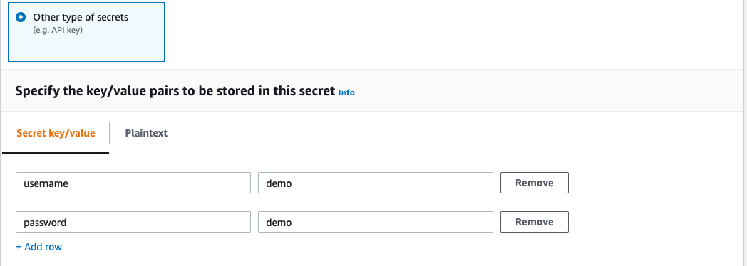
    5. Authentication: Choose either the database username and password credentials or AWS Secrets Manager. We recommend using AWS Secrets Manager.

After the connection is established, the federated catalog is created, as shown in the following screenshot. This catalog uses the AWS Glue connection to Amazon Redshift. The databases, tables, and views are automatically cataloged in the catalog section and registered with Lake Formation.

Verify the stores sales data

  1. Visit the Catalog section in SageMaker Unified Studio.
  2. Confirm that the retails sales public database and its tables (RETAIL_SALES, STORE, PRODUCT) are now available.

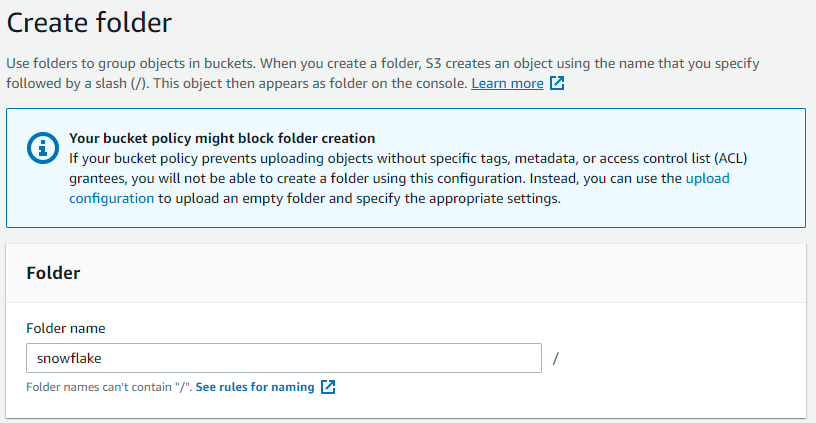
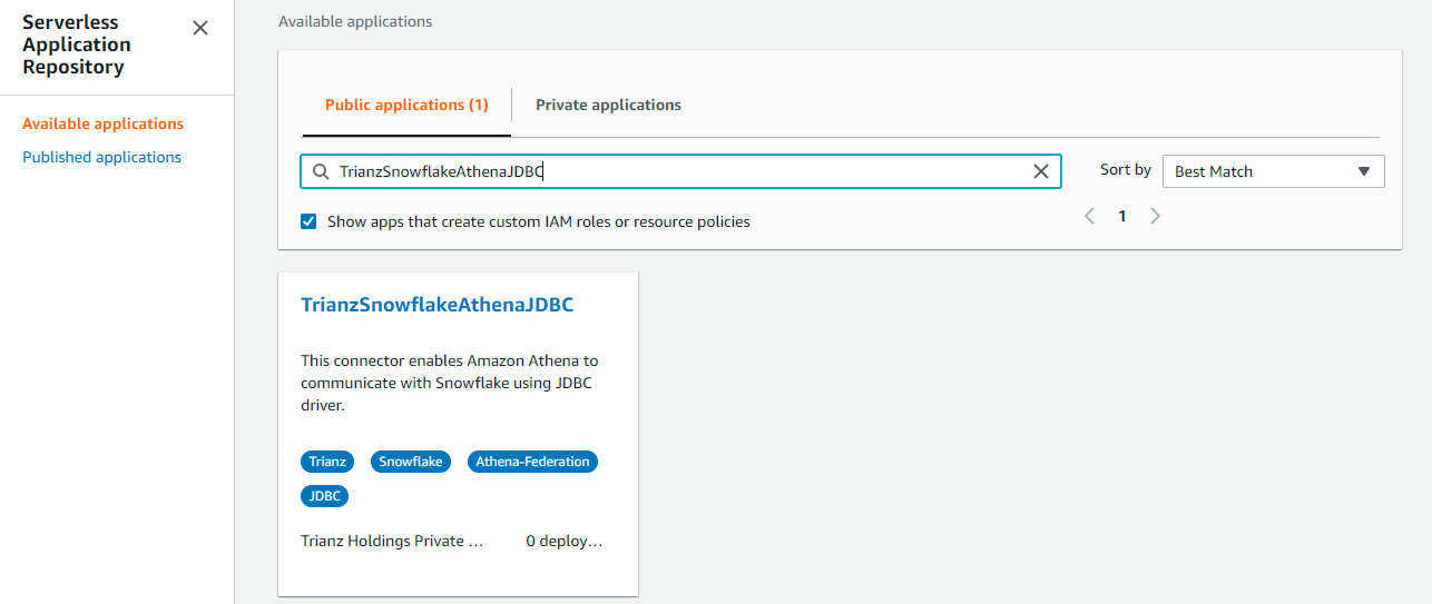
Connecting to Snowflake (online sales data)

In this step, we bring online sales data from Snowflake into Amazon SageMaker Unified Studio.

Create a federated connection for Snowflake

  1. In the Centralized Processing account, go to the SageMaker Unified Studio console, choose your project.
  2. Choose Data in the Navigation Pane.
  3. In the data explorer, choose the plus sign (+) to add a data source.
  4. Under Add a data source, choose Add connection, then choose Snowflake.
  5. Enter the following parameters in the connection details, and choose Add data.
    1. Name: Enter the connection name (such as anycompanysnowflake).
    2. Host: Enter the Snowflake cluster endpoint.
    3. Port: Enter the port number (Snowflake uses 443 as the default port).
    4. Database: Enter the database name (such as anycompanyonlinesales).
    5. Warehouse: Enter the warehouse name (such as COMPUTE_WH).
    6. Authentication: Choose either the database username and password credentials or Secrets Manager.

After the connection is established, the federated catalog is created for Snowflake. This catalog uses the AWS Glue connection to Snowflake. The databases, tables, and views are automatically cataloged in the Data Catalog and registered with Lake Formation.

Verify the online sales data

  1. Go to the Catalog section in SageMaker Unified Studio.
  2. Confirm that the Online sales public database and its tables (CUSTOMER_REVIEWS, CUSTOMER, ONLINE_SALES, PRODUCT) are now available.

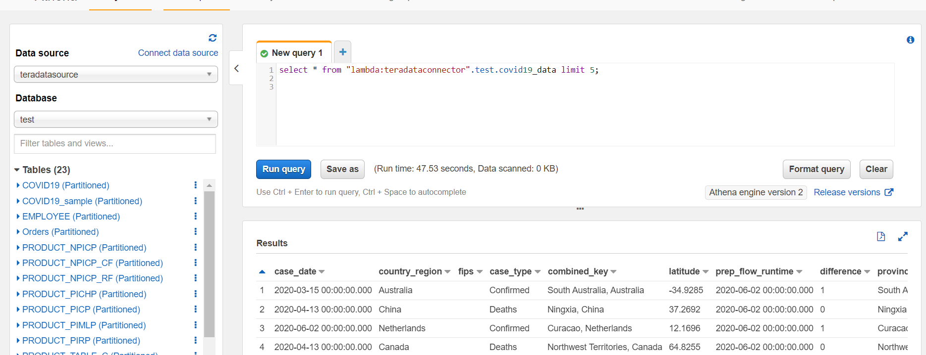
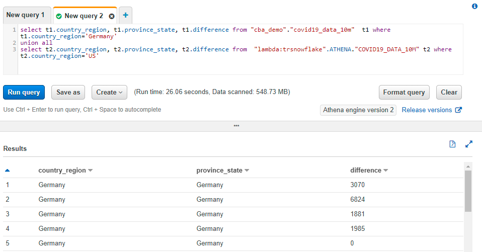
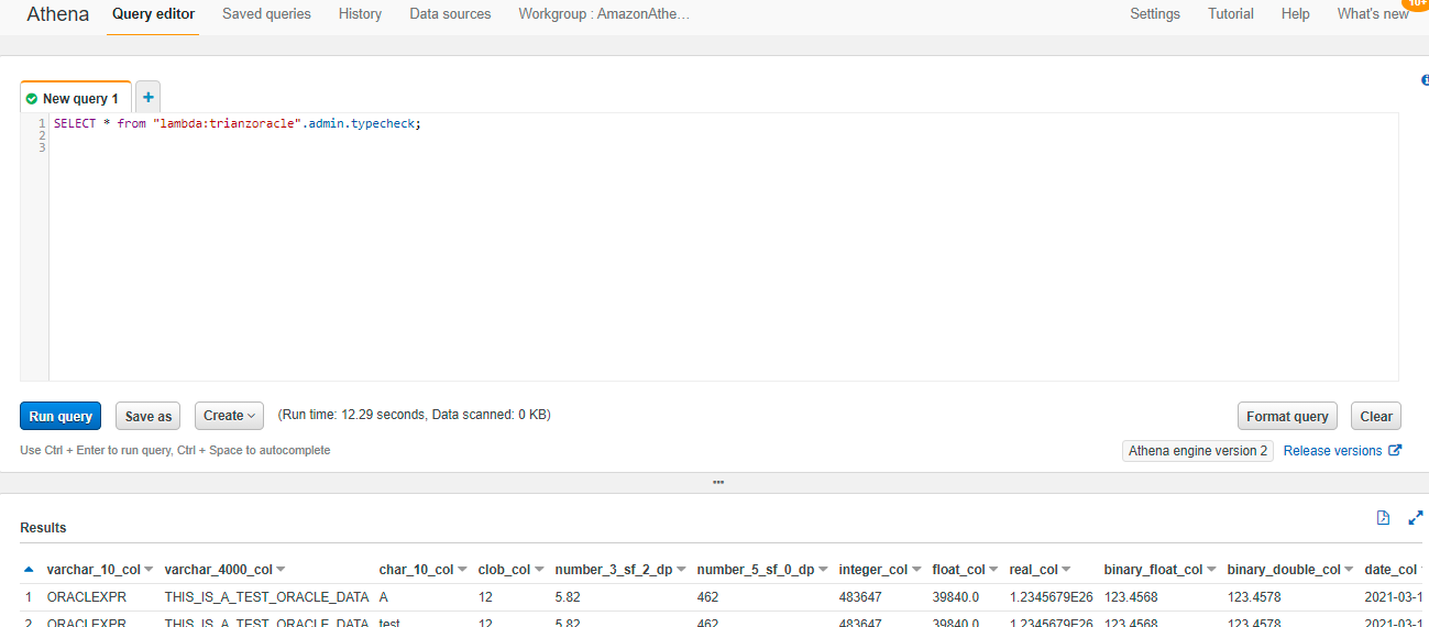
Step 3: Analyze the data together

Once all the data from different data sources has been cataloged, we can analyze it using Amazon Athena query engine from Amazon SageMaker Unified Studio.

  1. In the Centralized Processing account, go to the SageMaker Unified Studio console, choose your project.
  2. Choose Query Editor from the Build section.
  3. Select Athena (Lakehouse) as a connection.
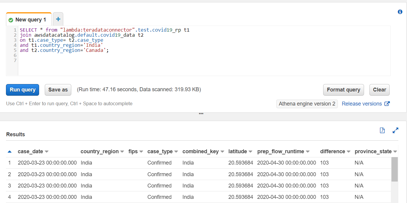
  4. Run queries joining multiple data source catalogs to analyze the data.

Example: What is the total revenue generated from wholesale, retail, and online sales for each product?

SELECT p.product_id, p.product_name, COALESCE(SUM(ws.total_revenue), 0) AS wholesale_revenue, COALESCE(SUM(rs.revenue), 0) AS retail_revenue, COALESCE(SUM(os.sale_price * os.quantity_sold), 0) AS online_revenue, (COALESCE(SUM(ws.total_revenue), 0) + COALESCE(SUM(rs.revenue), 0) + COALESCE(SUM(os.sale_price * os.quantity_sold), 0)) AS total_revenueFROM awsdatacatalog.anycompanydatacatalog.anycompany_products pLEFT JOIN awsdatacatalog.anycompanydatacatalog.anycompany_wholessale_sales ws ON p.product_id = ws.product_idLEFT JOIN anycompanyredshift.public.retail_sales rs ON p.product_id = rs.product_idLEFT JOIN anycompanysnowflake.sales.online_sales os ON p.product_id = os.product_idGROUP BY p.product_id, p.product_nameORDER BY total_revenue DESC;

Similarly, users can derive valuable business insights by querying across catalogs for different analytical questions.

Step 4: Creating a Business Glossary

A business glossary helps standardize terminology across the organization and makes data more discoverable. Now we create a business glossary for Wholesale data PRODUCT.

  1. In the Navigation Pane, choose Data and select Publish to Catalog for the Wholesale data PRODUCT table.
  2. Choose Assets and choose the products table.
  3. Create a Glossary named ‘Product‘ and a Term named ‘Sales‘ from Metadata entities.
  4. Choose Generate Descriptions to automatically generate summary of your data using AI. Choose Add Terms.
  5. Choose ACCEPT ALL for Automated Metadata Generation.
  6. Choose sales term and choose Add Terms.
  7. Choose Publish Asset.
  8. Choose Assets and then Published. We can now see a published asset that is searchable and available to request for subscription.

Similarly, you can create business glossaries for other data products by following the above steps.

Step 5: Setting up access controls

To ensure proper governance, set up fine-grained access controls.

  1. For each user create a new single sign-on (SSO) user
  2. Create the following roles and permissions to attach to the SSO user:
Role Description Access Level
Data Steward Manages the data catalog and glossary Full access to catalog and glossary
ETL Developer Develops data integration pipelines Read/write access to data sources and AWS Glue
Data Analyst Analyzes sales data Read-only access to all sales data
AI Engineer Builds forecasting models Read access to sales data, full access to SageMaker features

Benefits of SageMaker Catalog

By implementing a self-service business data catalog using Amazon SageMaker Unified Studio, our retail organization achieves several key benefits:

  1. Unified data access: Users can discover and access data from Amazon S3, Redshift, and Snowflake through a single interface.
  2. Standardized metadata: The business glossary ensures consistent terminology across the organization.
  3. Governance and compliance: Fine-grained access controls ensure that users only access data they’re authorized to see.
  4. Collaboration: Different teams (ETL developers, data analysts, AI engineers) can collaborate within a shared environment.

Cleanup

To avoid incurring additional charges associated with the resources created in this post, make sure to delete the following items from your AWS account:

  1. The Amazon SageMaker domain.
  2. The Amazon S3 bucket associated with the Amazon SageMaker domain.
  3. Cross-account resources such as VPC peering connections, security groups, route tables, AWS Glue Data Catalog entries, and associated IAM roles4. The tables and databases created in this post.

Conclusion

In this post, we demonstrated how Amazon SageMaker Catalog provides a unified approach to data publishing, discovery, and analysis across multiple data sources. Using a retail scenario, we showed how to import data from Amazon S3, Amazon Redshift, and Snowflake into Amazon SageMaker Unified Studio, and how to join and analyze data from these multiple sources to derive meaningful business insights.

By centralizing metadata and enabling cross-source data integration, data is easily discovered across an organization, multiple data sources can be joined and comprehensive analysis performed without moving or duplicating data. This unified approach maintains strong governance with consistent policies, security, and compliance across all data sources while enabling self-service analytics that reduce time-to-insight for your teams.

To learn more about Amazon SageMaker and how to get started, refer to the Amazon SageMaker User Guide.


About the authors

Navnit Shukla

Navnit Shukla

Navnit is an AWS Specialist Solutions Architect at AWS with a focus on Data and AI. He possesses a strong enthusiasm for assisting clients in discovering valuable insights from their data. Through his expertise, he constructs innovative solutions that empower businesses to arrive at informed, data-driven choices. Notably, he is the lead author of Data Wrangling on AWS and AI-Ready Data Blueprints with O’Reilly.

Ayan Majumder

Ayan Majumder

Ayan is an Analytics Specialist Solutions Architect at AWS. His expertise lies in designing robust, scalable, and efficient cloud solutions for customers. Beyond his professional life, he derives joy from traveling, photography, and outdoor activities.

Karan Edikala

Karan Edikala

Karan is a Solutions Architect at AWS who helps small businesses unlock value through cloud technology. He specializes in Generative AI, guiding customers to build AI-powered solutions that deliver measurable ROI and optimize their data strategies on AWS. Outside of work, Karan enjoys piloting general aviation aircraft, golfing, and skiing.

Accelerate queries on Apache Iceberg tables through AWS Glue auto compaction

Post Syndicated from Navnit Shukla original https://aws.amazon.com/blogs/big-data/accelerate-queries-on-apache-iceberg-tables-through-aws-glue-auto-compaction/

Data lakes were originally designed to store large volumes of raw, unstructured, or semi-structured data at a low cost, primarily serving big data and analytics use cases. Over time, as organizations began to explore broader applications, data lakes have become essential for various data-driven processes beyond just reporting and analytics. Today, they play a critical role in syncing with customer applications, enabling the ability to manage concurrent data operations while maintaining the integrity and consistency of information. This shift includes not only storing batch data but also ingesting and processing near real-time data streams, allowing businesses to merge historical insights with live data to power more responsive and adaptive decision-making. However, this new data lake architecture brings challenges around managing transactional support and handling the influx of small files generated by real-time data streams. Traditionally, customers addressed these challenges by performing complex extract, transform, and load (ETL) processes, which often led to data duplication and increased complexity in data pipelines. Additionally, to cope with the proliferation of small files, organizations had to develop custom mechanisms to compact and merge these files, leading to the creation and maintenance of bespoke solutions that were difficult to scale and manage. As data lakes increasingly handle sensitive business data and transactional workloads, maintaining strong data quality, governance, and compliance becomes vital to maintaining trust and regulatory alignment.

To simplify these challenges, organizations have adopted open table formats (OTFs) like Apache Iceberg, which provide built-in transactional capabilities and mechanisms for compaction. OTFs, such as Iceberg, address key limitations in traditional data lakes by offering features like ACID transactions, which maintain data consistency across concurrent operations, and compaction, which helps manage the issue of small files by merging them efficiently. By using features like Iceberg’s compaction, OTFs streamline maintenance, making it straightforward to manage object and metadata versioning at scale. However, although OTFs reduce the complexity of maintaining efficient tables, they still require some regular maintenance to make sure tables remain in an optimal state.

In this post, we explore new features of the AWS Glue Data Catalog, which now supports improved automatic compaction of Iceberg tables for streaming data, making it straightforward for you to keep your transactional data lakes consistently performant. Enabling automatic compaction on Iceberg tables reduces metadata overhead on your Iceberg tables and improves query performance. Many customers have streaming data continuously ingested in Iceberg tables, resulting in a large number of delete files that track changes in data files. With this new feature, as you enable the Data Catalog optimizer. It constantly monitors table partitions and runs the compaction process for both data and delta or delete files, and it regularly commits partial progress. The Data Catalog also now supports heavily nested complex data and supports schema evolution as you reorder or rename columns.

Automatic compaction with AWS Glue

Automatic compaction in the Data Catalog makes sure your Iceberg tables are always in optimal condition. The data compaction optimizer continuously monitors table partitions and invokes the compaction process when specific thresholds for the number of files and file sizes are met. For example, based on the Iceberg table configuration of the target file size, the compaction process will start and continue if the table or any of the partitions within the table have more than the default configuration (for example 100 files), each smaller than 75% of the target file size.

Iceberg supports two table modes: Merge-on-Read (MoR) and Copy-on-Write (CoW). These table modes provide different approaches for handling data updates and play a critical role in how data lakes manage changes and maintain performance:

  • Data compaction on Iceberg CoW – With CoW, any updates or deletes are directly applied to the table files. This means the entire dataset is rewritten when changes are made. Although this provides immediate consistency and simplifies reads (because readers only access the latest snapshot of the data), it can become costly and slow for write-heavy workloads due to the need for frequent rewrites. Announced during AWS re:Invent 2023, this feature focuses on optimizing data storage for Iceberg tables using the CoW mechanism. Compaction in CoW makes sure updates to the data result in new files being created, which are then compacted to improve query performance.
  • Data compaction on Iceberg MoR – Unlike CoW, MoR allows updates to be written separately from the existing dataset, and those changes are only merged when the data is read. This approach is beneficial for write-heavy scenarios because it avoids frequent full table rewrites. However, it can introduce complexity during reads because the system has to merge base and delta files as needed to provide a complete view of the data. MoR compaction, now generally available, allows for efficient handling of streaming data. It makes sure that while data is being continuously ingested, it’s also compacted in a way that optimizes read performance without compromising the ingestion speed.

Whether you are using CoW, MoR, or a hybrid of both, one challenge remains consistent: maintenance around the growing number of small files generated by each transaction. AWS Glue automatic compaction addresses this by making sure your Iceberg tables remain efficient and performant across both table modes.

This post provides a detailed comparison of query performance between auto compacted and non-compacted Iceberg tables. By analyzing key metrics such as query latency and storage efficiency, we demonstrate how the automatic compaction feature optimizes data lakes for better performance and cost savings. This comparison will help guide you in making informed decisions on enhancing your data lake environments.

Solution overview

This blog post explores the performance benefits of the newly launched feature in AWS Glue that supports automatic compaction of Iceberg tables with MoR capabilities. We run two versions of the same architecture: one where the tables are auto compacted, and another without compaction. By comparing both scenarios, this post demonstrates the efficiency, query performance, and cost benefits of auto compacted tables vs. non-compacted tables in a simulated Internet of Things (IoT) data pipeline.

The following diagram illustrates the solution architecture.

The solution consists of the following components:

  • Amazon Elastic Compute Cloud (Amazon EC2) simulates continuous IoT data streams, sending them to Amazon MSK for processing
  • Amazon Managed Streaming for Apache Kafka (Amazon MSK) ingests and streams data from the IoT simulator for real-time processing
  • Amazon EMR Serverless processes streaming data from Amazon MSK without managing clusters, writing results to the Amazon S3 data lake
  • Amazon Simple Storage Service (Amazon S3) stores data using Iceberg’s MoR format for efficient querying and analysis
  • The Data Catalog manages metadata for the datasets in Amazon S3, enabling organized data discovery and querying through Amazon Athena
  • Amazon Athena queries data from the S3 data lake with two table options:
    • Non-compacted table – Queries raw data from the Iceberg table
    • Compacted table – Queries data optimized by automatic compaction for faster performance.

The data flow consists of the following steps:

  1. The IoT simulator on Amazon EC2 generates continuous data streams.
  2. The data is sent to Amazon MSK, which acts as a streaming table.
  3. EMR Serverless processes streaming data and writes the output to Amazon S3 in Iceberg format.
  4. The Data Catalog manages the metadata for the datasets.
  5. Athena is used to query the data, either directly from the non-compacted table or from the compacted table after auto compaction.

In this post, we guide you through setting up an evaluation environment for AWS Glue Iceberg auto compaction performance using the following GitHub repository. The process involves simulating IoT data ingestion, deduplication, and querying performance using Athena.

Compaction IoT performance test

We simulated IoT data ingestion with over 20 billion events and used MERGE INTO for data deduplication across two time-based partitions, involving heavy partition reads and shuffling. After ingestion, we ran queries in Athena to compare performance between compacted and non-compacted tables using the MoR format. This test aims to have low latency on ingestion but will lead to hundreds of millions of small files.

We use the following table configuration settings:

'write.delete.mode'='merge-on-read'
'write.update.mode'='merge-on-read'
'write.merge.mode'='merge-on-read'
'write.distribution.mode=none'

We use 'write.distribution.mode=none' to lower the latency. However, it will increase the number of Parquet files. For other scenarios, you may want to use hash or range distribution write modes to reduce the file count.

This test makes make append operations because we’re appending new data to the table but we don’t have any delete operations.

The following table shows some metrics of the Athena query performance.


Execution Time (sec) Performance Improvement (%) Data Scanned (GB)
Query employee (without compaction) employeeauto (with compaction) employee (without compaction) employeeauto (with compaction)
SELECT count(*) FROM "bigdata"."<tablename>" 67.5896 3.8472 94.31% 0 0
SELECT team, name, min(age) AS youngest_age
FROM "bigdata"."<tablename>"
GROUP BY team, name
ORDER BY youngest_age ASC
72.0152 50.4308 29.97% 33.72 32.96
SELECT role, team, avg(age) AS average_age
FROM bigdata."<tablename>"
GROUP BY role, team
ORDER BY average_age DESC
74.1430 37.7676 49.06% 17.24 16.59
SELECT name, age, start_date, role, team
FROM bigdata."<tablename>"
WHERE
CAST(start_date as DATE) > CAST('2023-01-02' as DATE) and
age > 40
ORDER BY start_date DESC
limit 100
70.3376 37.1232 47.22% 105.74 110.32

Because the previous test didn’t perform any delete operations on the table, we conduct a new test involving hundreds of thousands of such operations. We use the previously auto compacted table (employeeauto) as a base, noting that this table uses MoR for all operations.

We run a query that deletes data from each even second on the table:

DELETE FROM iceberg_catalog.bigdata.employeeauto
WHERE start_date BETWEEN 'start' AND 'end'
AND SECOND(start_date) % 2 = 0;

This query runs with table optimizations enabled, using an Amazon EMR Studio notebook. After running the queries, we roll back the table to its previous state for a performance comparison. Iceberg’s time-traveling capabilities allow us to restore the table. We then disable the table optimizations, rerun the delete query, and follow up with Athena queries to analyze performance differences. The following table summarizes our results.


Execution Time (sec) Performance Improvement (%) Data Scanned (GB)
Query employee (without compaction) employeeauto (with compaction) employee (without compaction) employeeauto (with compaction)
SELECT count(*) FROM "bigdata"."<tablename>" 29.820 8.71 70.77% 0 0
SELECT team, name, min(age) as youngest_age
FROM "bigdata"."<tablename>"
GROUP BY team, name
ORDER BY youngest_age ASC
58.0600 34.1320 41.21% 33.27 19.13
SELECT role, team, avg(age) AS average_age
FROM bigdata."<tablename>"
GROUP BY role, team
ORDER BY average_age DESC
59.2100 31.8492 46.21% 16.75 9.73
SELECT name, age, start_date, role, team
FROM bigdata."<tablename>"
WHERE
CAST(start_date as DATE) > CAST('2023-01-02' as DATE) and
age > 40
ORDER BY start_date DESC
limit 100
68.4650 33.1720 51.55% 112.64 61.18

We analyze the following key metrics:

  • Query runtime – We compared the runtimes between compacted and non-compacted tables using Athena as the query engine and found significant performance improvements with both MoR for ingestion and appends and MoR for delete operations.
  • Data scanned evaluation – We compared compacted and non-compacted tables using Athena as the query engine and observed a reduction in data scanned for most queries. This reduction translates directly into cost savings.

Prerequisites

To set up your own evaluation environment and test the feature, you need the following prerequisites:

  • A virtual private cloud (VPC) with at least two private subnets. For instructions, see Create a VPC.
  • An EC2 instance c5.xlarge using Amazon Linux 2023 running on one of those private subnets where you will launch the data simulator. For the security group, you can use the default for the VPC. For more information, see Get started with Amazon EC2.
  • An AWS Identity and Access Management (IAM) user with the correct permissions to create and configure all the required resources.

Set up Amazon S3 storage

Create an S3 bucket with the following structure:

s3bucket/
/jars
/employee.desc
/warehouse
/checkpoint
/checkpointAuto

Download the descriptor file employee.desc from the GitHub repo and place it in the S3 bucket.

Download the application on the releases page

Get the packaged application from the GitHub repo, then upload the JAR file to the jars directory on the S3 bucket. The warehouse will be where the Iceberg data and metadata will live and checkpoint will be used for the Structured Streaming checkpointing mechanism. Because we use two streaming job runs, one for compacted and one for non-compacted data, we also create a checkpointAuto folder.

Create a Data Catalog database

Create a database in the Data Catalog (for this post, we name our database bigdata). For instructions, see Getting started with the AWS Glue Data Catalog.

Create an EMR Serverless application

Create an EMR Serverless application with the following settings (for instructions, see Getting started with Amazon EMR Serverless):

  • Type: Spark
  • Version: 7.1.0
  • Architecture: x86_64
  • Java Runtime: Java 17
  • Metastore Integration: AWS Glue Data Catalog
  • Logs: Enable Amazon CloudWatch Logs if desired

Configure the network (VPC, subnets, and default security group) to allow the EMR Serverless application to reach the MSK cluster.

Take note of the application-id to use later for launching the jobs.

Create an MSK cluster

Create an MSK cluster on the Amazon MSK console. For more details, see Get started using Amazon MSK.

You need to use custom create with at least two brokers using 3.5.1, Apache Zookeeper mode version, and instance type kafka.m7g.xlarge. Do not use public access; choose two private subnets to deploy it (one broker per subnet or Availability Zone, for a total of two brokers). For the security group, remember that the EMR cluster and the Amazon EC2 based producer will need to reach the cluster and act accordingly. For security, use PLAINTEXT (in production, you should secure access to the cluster). Choose 200 GB as storage size for each broker and do not enable tiered storage. For network security groups, you can choose the default of the VPC.

For the MSK cluster configuration, use the following settings:

auto.create.topics.enable=true
default.replication.factor=2
min.insync.replicas=2
num.io.threads=8
num.network.threads=5
num.partitions=32
num.replica.fetchers=2
replica.lag.time.max.ms=30000
socket.receive.buffer.bytes=102400
socket.request.max.bytes=104857600
socket.send.buffer.bytes=102400
unclean.leader.election.enable=true
zookeeper.session.timeout.ms=18000
compression.type=zstd
log.retention.hours=2
log.retention.bytes=10073741824

Configure the data simulator

Log in to your EC2 instance. Because it’s running on a private subnet, you can use an instance endpoint to connect. To create one, see Connect to your instances using EC2 Instance Connect Endpoint. After you log in, issue the following commands:

sudo yum install java-17-amazon-corretto-devel
wget https://archive.apache.org/dist/kafka/3.5.1/kafka_2.12-3.5.1.tgz
tar xzvf kafka_2.12-3.5.1.tgz

Create Kafka topics

Create two Kafka topics—remember that you need to change the bootstrap server with the corresponding client information. You can get this data from the Amazon MSK console on the details page for your MSK cluster.

cd kafka_2.12-3.5.1/bin/

./kafka-topics.sh --topic protobuf-demo-topic-pure-auto --bootstrap-server kafkaBoostrapString --create
./kafka-topics.sh --topic protobuf-demo-topic-pure --bootstrap-server kafkaBoostrapString –create

Launch job runs

Issue job runs for the non-compacted and auto compacted tables using the following AWS Command Line Interface (AWS CLI) commands. You can use AWS CloudShell to run the commands.

For the non-compacted table, you need to change the s3bucket value as needed and the application-id. You also need an IAM role (execution-role-arn) with the corresponding permissions to access the S3 bucket and to access and write tables on the Data Catalog.

aws emr-serverless start-job-run --application-id application-identifier --name job-run-name --execution-role-arn arn-of-emrserverless-role --mode 'STREAMING' --job-driver '{
"sparkSubmit": {
"entryPoint": "s3://s3bucket/jars/streaming-iceberg-ingest-1.0-SNAPSHOT.jar",
"entryPointArguments": ["true","s3://s3bucket/warehouse","s3://s3bucket/Employee.desc","s3://s3bucket/checkpoint","kafkaBootstrapString","true"],
"sparkSubmitParameters": "--class com.aws.emr.spark.iot.SparkCustomIcebergIngestMoR --conf spark.executor.cores=16 --conf spark.executor.memory=64g --conf spark.driver.cores=4 --conf spark.driver.memory=16g --conf spark.dynamicAllocation.minExecutors=3 --conf spark.jars=/usr/share/aws/iceberg/lib/iceberg-spark3-runtime.jar --conf spark.dynamicAllocation.maxExecutors=5 --conf spark.sql.catalog.glue_catalog.http-client.apache.max-connections=3000 --conf spark.emr-serverless.executor.disk.type=shuffle_optimized --conf spark.emr-serverless.executor.disk=1000G --files s3://s3bucket/Employee.desc --packages org.apache.spark:spark-sql-kafka-0-10_2.12:3.5.1"
}
}'

For the auto compacted table, you need to change the s3bucket value as needed, the application-id, and the kafkaBootstrapString. You also need an IAM role (execution-role-arn) with the corresponding permissions to access the S3 bucket and to access and write tables on the Data Catalog.

aws emr-serverless start-job-run --application-id application-identifier --name job-run-name --execution-role-arn arn-of-emrserverless-role --mode 'STREAMING' --job-driver '{
"sparkSubmit": {
"entryPoint": "s3://s3bucket/jars/streaming-iceberg-ingest-1.0-SNAPSHOT.jar",
"entryPointArguments": ["true","s3://s3bucket/warehouse","/home/hadoop/Employee.desc","s3://s3bucket/checkpointAuto","kafkaBootstrapString","true"],
"sparkSubmitParameters": "--class com.aws.emr.spark.iot.SparkCustomIcebergIngestMoRAuto --conf spark.executor.cores=16 --conf spark.executor.memory=64g --conf spark.driver.cores=4 --conf spark.driver.memory=16g --conf spark.dynamicAllocation.minExecutors=3 --conf spark.jars=/usr/share/aws/iceberg/lib/iceberg-spark3-runtime.jar --conf spark.dynamicAllocation.maxExecutors=5 --conf spark.sql.catalog.glue_catalog.http-client.apache.max-connections=3000 --conf spark.emr-serverless.executor.disk.type=shuffle_optimized --conf spark.emr-serverless.executor.disk=1000G --files s3://s3bucket/Employee.desc --packages org.apache.spark:spark-sql-kafka-0-10_2.12:3.5.1"
}
}'

Enable auto compaction

Enable auto compaction for the employeeauto table in AWS Glue. For instructions, see Enabling compaction optimizer.

Launch the data simulator

Download the JAR file to the EC2 instance and run the producer:

aws s3 cp s3://s3bucket/jars/streaming-iceberg-ingest-1.0-SNAPSHOT.jar .

Now you can start the protocol buffer producers.

For non-compacted tables, use the following commands:

java -cp streaming-iceberg-ingest-1.0-SNAPSHOT.jar 
com.aws.emr.proto.kafka.producer.ProtoProducer kafkaBoostrapString

For auto compacted tables, use the following commands:

java -cp streaming-iceberg-ingest-1.0-SNAPSHOT.jar 
com.aws.emr.proto.kafka.producer.ProtoProducerAuto kafkaBoostrapString

Test the solution in EMR Studio

For the delete test, we use an EMR Studio. For setup instructions, see Set up an EMR Studio. Next, you need to create an EMR Serverless interactive application to run the notebook; refer to Run interactive workloads with EMR Serverless through EMR Studio to create a Workspace.

Open the Workspace, select the interactive EMR Serverless application as the compute option, and attach it.

Download the Jupyter notebook, upload it to your environment, and run the cells using a PySpark kernel to run the test.

Clean up

This evaluation is for high-throughput scenarios and can lead to significant costs. Complete the following steps to clean up your resources:

  1. Stop the Kafka producer EC2 instance.
  2. Cancel the EMR job runs and delete the EMR Serverless application.
  3. Delete the MSK cluster.
  4. Delete the tables and database from the Data Catalog.
  5. Delete the S3 bucket.

Conclusion

The Data Catalog has improved automatic compaction of Iceberg tables for streaming data, making it straightforward for you to keep your transactional data lakes always performant. Enabling automatic compaction on Iceberg tables reduces metadata overhead on your Iceberg tables and improves query performance.

Many customers have streaming data that is continuously ingested in Iceberg tables, resulting in a large set of delete files that track changes in data files. With this new feature, when you enable the Data Catalog optimizer, it constantly monitors table partitions and runs the compaction process for both data and delta or delete files and regularly commits the partial progress. The Data Catalog also has expanded support for heavily nested complex data and supports schema evolution as you reorder or rename columns.

In this post, we assessed the ingestion and query performance of simulated IoT data using AWS Glue Iceberg with auto compaction enabled. Our setup processed over 20 billion events, managing duplicates and late-arriving events, and employed a MoR approach for both ingestion/appends and deletions to evaluate the performance improvement and efficiency.

Overall, AWS Glue Iceberg with auto compaction proves to be a robust solution for managing high-throughput IoT data streams. These enhancements lead to faster data processing, shorter query times, and more efficient resource utilization, all of which are essential for any large-scale data ingestion and analytics pipeline.

For detailed setup instructions, see the GitHub repo.


About the Authors

Navnit Shukla serves as an AWS Specialist Solutions Architect with a focus on Analytics. He possesses a strong enthusiasm for assisting clients in discovering valuable insights from their data. Through his expertise, he constructs innovative solutions that empower businesses to arrive at informed, data-driven choices. Notably, Navnit Shukla is the accomplished author of the book titled Data Wrangling on AWS. He can be reached through LinkedIn.

Angel Conde Manjon is a Sr. PSA Specialist on Data & AI, based in Madrid, and focuses on EMEA South and Israel. He has previously worked on research related to data analytics and artificial intelligence in diverse European research projects. In his current role, Angel helps partners develop businesses centered on data and AI.

Amit Singh currently serves as a Senior Solutions Architect at AWS, specializing in analytics and IoT technologies. With extensive expertise in designing and implementing large-scale distributed systems, Amit is passionate about empowering clients to drive innovation and achieve business transformation through AWS solutions.

Sandeep Adwankar is a Senior Technical Product Manager at AWS. Based in the California Bay Area, he works with customers around the globe to translate business and technical requirements into products that enable customers to improve how they manage, secure, and access data.

A customer’s journey with Amazon OpenSearch Ingestion pipelines

Post Syndicated from Navnit Shukla original https://aws.amazon.com/blogs/big-data/a-customers-journey-with-amazon-opensearch-ingestion-pipelines/

This is a guest post co-written with Mike Mosher, Sr. Principal Cloud Platform Network Architect at a multi-national financial credit reporting company.

I work for a multi-national financial credit reporting company that offers credit risk, fraud, targeted marketing, and automated decisioning solutions. We are an AWS early adopter and have embraced the cloud to drive digital transformation efforts. Our Cloud Center of Excellence (CCoE) team operates a global AWS Landing Zone, which includes a centralized AWS network infrastructure. We are also an AWS PrivateLink Ready Partner and offer our E-Connect solution to allow our B2B customers to connect to a range of products through private, secure, and performant connectivity.

Our E-Connect solution is a platform comprised of multiple AWS services like Application Load Balancer (ALB), Network Load Balancer (NLB), Gateway Load Balancer (GWLB), AWS Transit Gateway, AWS PrivateLink, AWS WAF, and third-party security appliances. All of these services and resources, as well as the large amount of network traffic across the platform, create a large number of logs, and we needed a solution to aggregate and organize these logs for quick analysis by our operations teams when troubleshooting the platform.

Our original design consisted of Amazon OpenSearch Service, selected for its ability to return specific log entries from extensive datasets in seconds. We also complemented this with Logstash, allowing us to use multiple filters to enrich and augment the data before sending to the OpenSearch cluster, facilitating a more comprehensive and insightful monitoring experience.

In this post, we share our journey, including the hurdles we faced, the solutions we thought about, and why we went with Amazon OpenSearch Ingestion pipelines to make our log management smoother.

Overview of the initial solution

We originally wanted to store and analyze the logs in an OpenSearch cluster, and decided to use the AWS-managed service for OpenSearch called Amazon OpenSearch Service. We also wanted to enrich these logs with Logstash, but there was no AWS-managed service for this, so we needed to deploy the application on an Amazon Elastic Compute Cloud (Amazon EC2) server. This setup meant that we had to implement a lot of maintenance of the server, including using AWS CodePipeline and AWS CodeDeploy to push new Logstash configurations to the server and restart the service. We also needed to perform server maintenance tasks such as patching and updating the operating system (OS) and the Logstash application, and monitor server resources such as Java heap, CPU, memory, and storage.

The complexity extended to validating the network path from the Logstash server to the OpenSearch cluster, incorporating checks on Access Control Lists (ACLs) and security groups, as well as routes in the VPC subnets. Scaling beyond a single EC2 server introduced considerations for managing an auto scaling group, Amazon Simple Queue Service (Amazon SQS) queues, and more. Maintaining the continuous functionality of our solution became a significant effort, diverting focus from the core tasks of operating and monitoring the platform.

The following diagram illustrates our initial architecture.

Possible solutions for us:

Our team looked at multiple options to manage the logs from this platform. We possess a Splunk solution for storing and analyzing logs, and we did assess it as a potential competitor to OpenSearch Service. However, we opted against it for several reasons:

  • Our team is more familiar with OpenSearch Service and Logstash than Splunk.
  • Amazon OpenSearch Service, being a managed service in AWS, facilitates a smoother log transfer process compared to our on-premises Splunk solution. Also, transporting logs to the on-premises Splunk cluster would incur high costs, consume bandwidth on our AWS Direct Connect connections, and introduce unnecessary complexity.
  • Splunk’s pricing structure, based on storage in GBs, proved cost-prohibitive for the volume of logs we intended to store and analyze.

Initial designs for an OpenSearch Ingestion pipeline solution

The Amazon team approached me about a new feature they were launching: Amazon OpenSearch Ingestion. This feature offered a great solution to the problems we were facing with managing EC2 instances for Logstash. First, the new feature removed all the heavy lifting from our team of managing multiple EC2 instances, scaling the servers up and down based on traffic, and monitoring the ingestion of logs and the resources of the underlying servers. Second, Amazon OpenSearch Ingestion pipelines supported most if not all of the Logstash filters we were using in our current solution, which allowed us to use the same functionality of our current solution for enriching the logs.

We were thrilled to be accepted into the AWS beta program, emerging as one of its earliest and largest adopters. Our journey began with ingesting VPC flow logs for our internet ingress platform, alongside Transit Gateway flow logs connecting all VPCs in the AWS Region. Handling such a substantial volume of logs proved to be a significant task, with Transit Gateway flow logs alone reaching upwards of 14 TB per day. As we expanded our scope to include other logs like ALB and NLB access logs and AWS WAF logs, the scale of the solution translated to higher costs.

However, our enthusiasm was somewhat dampened by the challenges we faced initially. Despite our best efforts, we encountered performance issues with the domain. Through collaborative efforts with the AWS team, we uncovered misconfigurations within our setup. We had been using instances that were inadequately sized for the volume of data we were handling. Consequently, these instances were constantly operating at maximum CPU capacity, resulting in a backlog of incoming logs. This bottleneck cascaded into our OpenSearch Ingestion pipelines, forcing them to scale up unnecessarily, even as the OpenSearch cluster struggled to keep pace.

These challenges led to a suboptimal performance from our cluster. We found ourselves unable to analyze flow logs or access logs promptly, sometimes waiting days after their creation. Additionally, the costs associated with these inefficiencies far exceeded our initial expectations.

However, with the assistance of the AWS team, we successfully addressed these issues, optimizing our setup for improved performance and cost-efficiency. This experience underscored the importance of proper configuration and collaboration in maximizing the potential of AWS services, ultimately leading to a more positive outcome for our data ingestion processes.

Optimized design for our OpenSearch Ingestion pipelines solution

We collaborated with AWS to enhance our overall solution, building a solution that is both high performing, cost-effective, and aligned with our monitoring requirements. The solution involves selectively ingesting specific log fields into the OpenSearch Service domain using an Amazon S3 Select pipeline in the pipeline source; alternative selective ingestion can also be done by filtering within pipelines. You can use include_keys and exclude_keys in your sink to filter data that’s routed to destination. We also used the built-in Index State Management feature to remove logs older than a predefined period to reduce the overall cost of the cluster.

The ingested logs in OpenSearch Service empower us to derive aggregate data, providing insights into trends and issues across the entire platform. For additional detailed analysis of these logs including all original log fields, we use Amazon Athena tables with partitioning to quickly and cost-effectively query Amazon Simple Storage Service (Amazon S3) for logs stored in Parquet format.

This comprehensive solution significantly enhances our platform visibility, reduces overall monitoring costs for handling a large log volume, and expedites our time to identify root causes when troubleshooting platform incidents.

The following diagram illustrates our optimized architecture.

Performance comparison

The following table compares the performance of the initial design with Logstash on Amazon EC2, the original OpenSearch Ingestion pipeline solution, and the optimized OpenSearch Ingestion pipeline solution.

  Initial Design with Logstash on Amazon EC2 Original Ingestion Pipeline Solution Optimized Ingestion Pipeline Solution
Maintenance Effort High: Solution required the team to manage multiple services and instances, taking effort away from managing and monitoring our platform. Low: OpenSearch Ingestion managed most of the undifferentiated heavy lifting, leaving the team to only maintain the ingestion pipeline configuration file. Low: OpenSearch Ingestion managed most of the undifferentiated heavy lifting, leaving the team to only maintain the ingestion pipeline configuration file.
Performance High: EC2 instances with Logstash could scale up and down as needed in the auto scaling group. Low: Due to insufficient resources on the OpenSearch cluster, the ingestion pipelines were constantly at max OpenSearch Compute Units (OCUs), causing log delivery to be delayed by multiple days. High: Ingestion pipelines can scale up and down in OCUs as needed.
Real-time Log Availability Medium: In order to pull, process, and deliver the large number of logs in Amazon S3, we needed a large number of EC2 instances. To save on cost, we ran fewer instances, which led to slower log delivery to OpenSearch. Low: Due to insufficient resources on the OpenSearch cluster, the ingestion pipelines were constantly at max OCUs, causing log delivery to be delayed by multiple days. High: The optimized solution was able to deliver a large number of logs to OpenSearch to be analyzed in near real time.
Cost Saving Medium: Running multiple services and instances to send logs to OpenSearch increased the cost of the overall solution. Low: Due to insufficient resources on the OpenSearch cluster, the ingestion pipelines were constantly at max OCUs, increasing the cost of the service. High: The optimized solution was able to scale the ingestion pipeline OCUs up and down as needed, which kept the overall cost low.
Overall Benefit Medium Low High

Conclusion

In this post, we highlighted my journey to build a solution using OpenSearch Service and OpenSearch Ingestion pipelines. This solution allows us to focus on analyzing logs and supporting our platform, without needing to support the infrastructure to deliver logs to OpenSearch. We also highlighted the need to optimize the service in order to increase performance and reduce cost.

As our next steps, we aim to explore the recently announced Amazon OpenSearch Service zero-ETL integration with Amazon S3 (in preview) feature within OpenSearch Service. This step is intended to further reduce the solution’s costs and provide flexibility in the timing and number of logs that are ingested.


About the Authors

Navnit Shukla serves as an AWS Specialist Solutions Architect with a focus on analytics. He possesses a strong enthusiasm for assisting clients in discovering valuable insights from their data. Through his expertise, he constructs innovative solutions that empower businesses to arrive at informed, data-driven choices. Notably, Navnit Shukla is the accomplished author of the book titled “Data Wrangling on AWS.” He can be reached via LinkedIn.

Mike Mosher is s Senior Principal Cloud Platform Network Architect at a multi-national financial credit reporting company. He has more than 16 years of experience in on-premises and cloud networking and is passionate about building new architectures on the cloud that serve customers and solve problems. Outside of work, he enjoys time with his family and traveling back home to the mountains of Colorado.

Revolutionizing data querying: Amazon Redshift and Visual Studio Code integration

Post Syndicated from Navnit Shukla original https://aws.amazon.com/blogs/big-data/revolutionizing-data-querying-amazon-redshift-and-visual-studio-code-integration/

In today’s data-driven landscape, the efficiency and accessibility of querying tools play a crucial role in driving businesses forward. Amazon Redshift recently announced integration with Visual Studio Code (), an action that transforms the way data practitioners engage with Amazon Redshift and reshapes your interactions and practices in data management. This innovation not only unlocks new possibilities, but also tackles long-standing challenges in data analytics and query handling.

While the Amazon Redshift query editor v2 (QE v2) offers a smooth experience for data analysts and business users, many organizations have data engineers and developers who rely on VS Code as their primary development tool. Traditionally, they had to use QE v2 for their development tasks, which wasn’t the most optimal solution. However, this new feature resolves that issue by enabling data engineers and developers to seamlessly integrate their development work within VS Code, enhancing their workflow efficiency.

Visual Studio Code’s integration simplifies access to database objects within Redshift data warehouses, offering an interface you’re already familiar with to run and troubleshoot your code.

By integrating Amazon Redshift Provisioned cluster, and Amazon Redshift Serverless with the popular and free VS Code, you can alleviate concerns about costs associated with third-party tools. This integration allows you to reduce or eliminate licensing expenses for query authoring and data visualization, because these functionalities are now available within the free VSCode editor.

The support for Amazon Redshift within VS Code marks a significant leap towards a more streamlined, cost-effective, and user-friendly data querying experience.

In this post, we explore how to kickstart your journey with Amazon Redshift using the AWS Toolkit for VS Code.

Solution overview

This post outlines the procedure for creating a secure and direct connection between your local VS Code environment and the Redshift cluster. Emphasizing both security and accessibility, this solution allows you to operate within the familiar VS Code interface while seamlessly engaging with your Redshift database.

The following diagram illustrates the VS Code connection to Amazon Redshift deployed in a private VPC.

To connect to a data warehouse using VS Code from the Toolkit, you can choose from the following methods:

  • Use a database user name and password
  • Use AWS Secrets Manager
  • Use temporary credentials (this option is only available with Amazon Redshift Provisioned cluster)

In the following sections, we show how to establish a connection with a database situated on an established provisioned cluster or a serverless data warehouse from the Toolkit.

Prerequisites

Before you begin using Amazon Redshift Provisioned Cluster  and Amazon Redshift Serverless with the AWS Toolkit for Visual Studio Code, make sure you’ve completed the following requirements:

  1. Connect to your AWS account using the Toolkit.
  2. Set up a Amazon Redshift or Amazon Redshift serverless data warehouse.

Establish a connection to your data warehouse using user credentials

To connect using the database user name and password, complete the following steps:

  1. Navigate through the Toolkit explorer, expanding the AWS Region housing your data warehouse (for example, US East (N. Virginia)).
  2. In the Toolkit, expand the Redshift section and choose your specific data warehouse.
  3. In the Select a Connection Type dialog, choose Database user name and password and provide the necessary information requested by the prompts.

After the Toolkit establishes the connection to your data warehouse, you will be able to view your available databases, tables, and schemas directly in the Toolkit explorer.

Establish a connection to your data warehouse using Secrets Manager

To connect using Secrets Manager, complete the following steps:

  1. Navigate through the Toolkit explorer, expanding the AWS Region housing your data warehouse.
  2. In the Toolkit, expand the Redshift section and choose your specific data warehouse.
  3. In the Select a Connection Type dialog, choose Secrets Manager and fill in the information requested at each prompt.

After the Toolkit establishes a successful connection to your data warehouse, you’ll gain visibility into your databases, tables, and schemas directly in the Toolkit explorer.

Establish a connection to your Amazon Redshift Provisioned cluster using Temporary credentials:

To connect using Temporary credentials complete the following steps:

  1. Navigate through the Toolkit explorer, expanding the AWS Region housing your data warehouse.
  2. In the Toolkit, expand the Redshift section and choose your specific data warehouse.
  3. In the Select a Connection Type dialog, choose Temporary Credentials and fill in the information requested at each prompt.

Run SQL statements

We have successfully established the connection. The next step involves running some SQL. The steps outlined in this section detail the process of generating and running SQL statements within your database using the Toolkit for Visual Studio Code.

  1. Navigate to the Toolkit explorer and expand Redshift, then choose the data warehouse that stores the desired database for querying.
  2. Choose Create Notebook and specify a file name and location for saving your notebook locally.
  3. Choose OK to open the notebook in your VS Code editor.
  4. Enter the following SQL statements into the VS Code editor, which will be stored in this notebook:
    create table promotion
    (
        p_promo_sk                integer               not null,
        p_promo_id                char(16)              not null,
        p_start_date_sk           integer                       ,
        p_end_date_sk             integer                       ,
        p_item_sk                 integer                       ,
        p_cost                    decimal(15,2)                 ,
        p_response_target         integer                       ,
        p_promo_name              char(50)                      ,
        p_channel_dmail           char(1)                       ,
        p_channel_email           char(1)                       ,
        p_channel_catalog         char(1)                       ,
        p_channel_tv              char(1)                       ,
        p_channel_radio           char(1)                       ,
        p_channel_press           char(1)                       ,
        p_channel_event           char(1)                       ,
        p_channel_demo            char(1)                       ,
        p_channel_details         varchar(100)                  ,
        p_purpose                 char(15)                      ,
        p_discount_active         char(1)                       ,
        primary key (p_promo_sk)
    ) diststyle all;
    
    create table reason
    (
        r_reason_sk               integer               not null,
        r_reason_id               char(16)              not null,
        r_reason_desc             char(100)                     ,
        primary key (r_reason_sk)
    ) diststyle all ;
    
    
    create table ship_mode
    (
        sm_ship_mode_sk           integer               not null,
        sm_ship_mode_id           char(16)              not null,
        sm_type                   char(30)                      ,
        sm_code                   char(10)                      ,
        sm_carrier                char(20)                      ,
        sm_contract               char(20)                      ,
        primary key (sm_ship_mode_sk)
    ) diststyle all;
    
    
    copy promotion from 's3://redshift-downloads/TPC-DS/2.13/1TB/promotion/' iam_role default gzip delimiter '|' EMPTYASNULL region 'us-east-1';
    copy reason from 's3://redshift-downloads/TPC-DS/2.13/1TB/reason/' iam_role default gzip delimiter '|' EMPTYASNULL region 'us-east-1';
    copy ship_mode from 's3://redshift-downloads/TPC-DS/2.13/1TB/ship_mode/' iam_role default gzip delimiter '|' EMPTYASNULL region 'us-east-1';
    
    
    select * from promotion limit 10;
    
    drop table promotion;
    drop table reason;
    drop table ship_mode;

  5. Choose Run All to run the SQL statements.

The output corresponding to your SQL statements will be visible below the entered statements within the editor.

Include markdown in a notebook

To include markdown in your notebook, complete the following steps:

  1. Access your notebook within the VS Code editor and choose Markdown to create a markdown cell.
  2. Enter your markdown content within the designated cell.
  3. Use the editing tools in the upper-right corner of the markdown cell to modify the markdown content as needed.

Congratulations, you have learned the art of using the VS Code editor to effectively interface with your Redshift environment.

Clean up

To remove the connection, complete the following steps:

  1. In the Toolkit explorer, expand Redshift, and choose the data warehouse containing your database.
  2. Choose the database (right-click) and choose Delete Connection.

Conclusion

In this post, we explored the process of using VS Code to establish a connection with Amazon Redshift, streamlining access to database objects within Redshift data warehouses.

You can learn about Amazon Redshift from Getting started with Amazon Redshift guide. Know more about write and run SQL queries directly in VS Code with the new AWS Toolkit for VS Code integration.


About the Author

Navnit Shukla, an AWS Specialist Solution Architect specializing in Analytics, is passionate about helping clients uncover valuable insights from their data. Leveraging his expertise, he develops inventive solutions that empower businesses to make informed, data-driven decisions. Notably, Navnit Shukla is the accomplished author of the book “Data Wrangling on AWS,” showcasing his expertise in the field.

Process and analyze highly nested and large XML files using AWS Glue and Amazon Athena

Post Syndicated from Navnit Shukla original https://aws.amazon.com/blogs/big-data/process-and-analyze-highly-nested-and-large-xml-files-using-aws-glue-and-amazon-athena/

In today’s digital age, data is at the heart of every organization’s success. One of the most commonly used formats for exchanging data is XML. Analyzing XML files is crucial for several reasons. Firstly, XML files are used in many industries, including finance, healthcare, and government. Analyzing XML files can help organizations gain insights into their data, allowing them to make better decisions and improve their operations. Analyzing XML files can also help in data integration, because many applications and systems use XML as a standard data format. By analyzing XML files, organizations can easily integrate data from different sources and ensure consistency across their systems, However, XML files contain semi-structured, highly nested data, making it difficult to access and analyze information, especially if the file is large and has complex, highly nested schema.

XML files are well-suited for applications, but they may not be optimal for analytics engines. In order to enhance query performance and enable easy access in downstream analytics engines such as Amazon Athena, it’s crucial to preprocess XML files into a columnar format like Parquet. This transformation allows for improved efficiency and usability in analytics workflows. In this post, we show how to process XML data using AWS Glue and Athena.

Solution overview

We explore two distinct techniques that can streamline your XML file processing workflow:

  • Technique 1: Use an AWS Glue crawler and the AWS Glue visual editor – You can use the AWS Glue user interface in conjunction with a crawler to define the table structure for your XML files. This approach provides a user-friendly interface and is particularly suitable for individuals who prefer a graphical approach to managing their data.
  • Technique 2: Use AWS Glue DynamicFrames with inferred and fixed schemas – The crawler has a limitation when it comes to processing a single row in XML files larger than 1 MB. To overcome this restriction, we use an AWS Glue notebook to construct AWS Glue DynamicFrames, utilizing both inferred and fixed schemas. This method ensures efficient handling of XML files with rows exceeding 1 MB in size.

In both approaches, our ultimate goal is to convert XML files into Apache Parquet format, making them readily available for querying using Athena. With these techniques, you can enhance the processing speed and accessibility of your XML data, enabling you to derive valuable insights with ease.

Prerequisites

Before you begin this tutorial, complete the following prerequisites (these apply to both techniques):

  1. Download the XML files technique1.xml and technique2.xml.
  2. Upload the files to an Amazon Simple Storage Service (Amazon S3) bucket. You can upload them to the same S3 bucket in different folders or to different S3 buckets.
  3. Create an AWS Identity and Access Management (IAM) role for your ETL job or notebook as instructed in Set up IAM permissions for AWS Glue Studio.
  4. Add an inline policy to your role with the iam:PassRole action:
  "Version": "2012-10-17",
  "Statement": [
    {
      "Action": ["iam:PassRole"],
      "Effect": "Allow",
      "Resource": "arn:aws:iam::*:role/AWSGlueServiceRole*",
      "Condition": {
        "StringLike": {
          "iam:PassedToService": ["glue.amazonaws.com"]
        }
      }
    }
}
  1. Add a permissions policy to the role with access to your S3 bucket.

Now that we’re done with the prerequisites, let’s move on to implementing the first technique.

Technique 1: Use an AWS Glue crawler and the visual editor

The following diagram illustrates the simple architecture that you can use to implement the solution.

Processing and Analyzing XML file using AWS Glue and Amazon Athena

To analyze XML files stored in Amazon S3 using AWS Glue and Athena, we complete the following high-level steps:

  1. Create an AWS Glue crawler to extract XML metadata and create a table in the AWS Glue Data Catalog.
  2. Process and transform XML data into a format (like Parquet) suitable for Athena using an AWS Glue extract, transform, and load (ETL) job.
  3. Set up and run an AWS Glue job via the AWS Glue console or the AWS Command Line Interface (AWS CLI).
  4. Use the processed data (in Parquet format) with Athena tables, enabling SQL queries.
  5. Use the user-friendly interface in Athena to analyze the XML data with SQL queries on your data stored in Amazon S3.

This architecture is a scalable, cost-effective solution for analyzing XML data on Amazon S3 using AWS Glue and Athena. You can analyze large datasets without complex infrastructure management.

We use the AWS Glue crawler to extract XML file metadata. You can choose the default AWS Glue classifier for general-purpose XML classification. It automatically detects XML data structure and schema, which is useful for common formats.

We also use a custom XML classifier in this solution. It’s designed for specific XML schemas or formats, allowing precise metadata extraction. This is ideal for non-standard XML formats or when you need detailed control over classification. A custom classifier ensures only necessary metadata is extracted, simplifying downstream processing and analysis tasks. This approach optimizes the use of your XML files.

The following screenshot shows an example of an XML file with tags.

Create a custom classifier

In this step, you create a custom AWS Glue classifier to extract metadata from an XML file. Complete the following steps:

  1. On the AWS Glue console, under Crawlers in the navigation pane, choose Classifiers.
  2. Choose Add classifier.
  3. Select XML as the classifier type.
  4. Enter a name for the classifier, such as blog-glue-xml-contact.
  5. For Row tag, enter the name of the root tag that contains the metadata (for example, metadata).
  6. Choose Create.

Create an AWS Glue Crawler to crawl xml file

In this section, we are creating a Glue Crawler to extract the metadata from XML file using the customer classifier created in previous step.

Create a database

  1. Go to the AWS Glue console, choose Databases in the navigation pane.
  2. Click on Add database.
  3. Provide a name such as blog_glue_xml
  4. Choose Create Database

Create a Crawler

Complete the following steps to create your first crawler:

  1. On the AWS Glue console, choose Crawlers in the navigation pane.
  2. Choose Create crawler.
  3. On the Set crawler properties page, provide a name for the new crawler (such as blog-glue-parquet), then choose Next.
  4. On the Choose data sources and classifiers page, select Not Yet under Data source configuration.
  5. Choose Add a data store.
  6. For S3 path, browse to s3://${BUCKET_NAME}/input/geologicalsurvey/.

Make sure you pick the XML folder rather than the file inside the folder.

  1. Leave the rest of the options as default and choose Add an S3 data source.
  2. Expand Custom classifiers – optional, choose blog-glue-xml-contact, then choose Next and keep the rest of the options as default.
  3. Choose your IAM role or choose Create new IAM role, add the suffix glue-xml-contact (for example, AWSGlueServiceNotebookRoleBlog), and choose Next.
  4. On the Set output and scheduling page, under Output configuration, choose blog_glue_xml for Target database.
  5. Enter console_ as the prefix added to tables (optional) and under Crawler schedule, keep the frequency set to On demand.
  6. Choose Next.
  7. Review all the parameters and choose Create crawler.

Run the Crawler

After you create the crawler, complete the following steps to run it:

  1. On the AWS Glue console, choose Crawlers in the navigation pane.
  2. Open the crawler you created and choose Run.

The crawler will take 1–2 minutes to complete.

  1. When the crawler is complete, choose Databases in the navigation pane.
  2. Choose the database you crated and choose the table name to see the schema extracted by the crawler.

Create an AWS Glue job to convert the XML to Parquet format

In this step, you create an AWS Glue Studio job to convert the XML file into a Parquet file. Complete the following steps:

  1. On the AWS Glue console, choose Jobs in the navigation pane.
  2. Under Create job, select Visual with a blank canvas.
  3. Choose Create.
  4. Rename the job to blog_glue_xml_job.

Now you have a blank AWS Glue Studio visual job editor. On the top of the editor are the tabs for different views.

  1. Choose the Script tab to see an empty shell of the AWS Glue ETL script.

As we add new steps in the visual editor, the script will be updated automatically.

  1. Choose the Job details tab to see all the job configurations.
  2. For IAM role, choose AWSGlueServiceNotebookRoleBlog.
  3. For Glue version, choose Glue 4.0 – Support Spark 3.3, Scala 2, Python 3.
  4. Set Requested number of workers to 2.
  5. Set Number of retries to 0.
  6. Choose the Visual tab to go back to the visual editor.
  7. On the Source drop-down menu, choose AWS Glue Data Catalog.
  8. On the Data source properties – Data Catalog tab, provide the following information:
    1. For Database, choose blog_glue_xml.
    2. For Table, choose the table that starts with the name console_ that the crawler created (for example, console_geologicalsurvey).
  9. On the Node properties tab, provide the following information:
    1. Change Name to geologicalsurvey dataset.
    2. Choose Action and the transformation Change Schema (Apply Mapping).
    3. Choose Node properties and change the name of the transform from Change Schema (Apply Mapping) to ApplyMapping.
    4. On the Target menu, choose S3.
  10. On the Data source properties – S3 tab, provide the following information:
    1. For Format, select Parquet.
    2. For Compression Type, select Uncompressed.
    3. For S3 source type, select S3 location.
    4. For S3 URL, enter s3://${BUCKET_NAME}/output/parquet/.
    5. Choose Node Properties and change the name to Output.
  11. Choose Save to save the job.
  12. Choose Run to run the job.

The following screenshot shows the job in the visual editor.

Create an AWS Gue Crawler to crawl the Parquet file

In this step, you create an AWS Glue crawler to extract metadata from the Parquet file you created using an AWS Glue Studio job. This time, you use the default classifier. Complete the following steps:

  1. On the AWS Glue console, choose Crawlers in the navigation pane.
  2. Choose Create crawler.
  3. On the Set crawler properties page, provide a name for the new crawler, such as blog-glue-parquet-contact, then choose Next.
  4. On the Choose data sources and classifiers page, select Not Yet for Data source configuration.
  5. Choose Add a data store.
  6. For S3 path, browse to s3://${BUCKET_NAME}/output/parquet/.

Make sure you pick the parquet folder rather than the file inside the folder.

  1. Choose your IAM role created during the prerequisite section or choose Create new IAM role (for example, AWSGlueServiceNotebookRoleBlog), and choose Next.
  2. On the Set output and scheduling page, under Output configuration, choose blog_glue_xml for Database.
  3. Enter parquet_ as the prefix added to tables (optional) and under Crawler schedule, keep the frequency set to On demand.
  4. Choose Next.
  5. Review all the parameters and choose Create crawler.

Now you can run the crawler, which takes 1–2 minutes to complete.

You can preview the newly created schema for the Parquet file in the AWS Glue Data Catalog, which is similar to the schema of the XML file.

We now possess data that is suitable for use with Athena. In the next section, we perform data queries using Athena.

Query the Parquet file using Athena

Athena doesn’t support querying the XML file format, which is why you converted the XML file into Parquet for more efficient data querying and use dot notation to query complex types and nested structures.

The following example code uses dot notation to query nested data:

SELECT 
    idinfo.citation.citeinfo.origin,
    idinfo.citation.citeinfo.pubdate,
    idinfo.citation.citeinfo.title,
    idinfo.citation.citeinfo.geoform,
    idinfo.citation.citeinfo.pubinfo.pubplace,
    idinfo.citation.citeinfo.pubinfo.publish,
    idinfo.citation.citeinfo.onlink,
    idinfo.descript.abstract,
    idinfo.descript.purpose,
    idinfo.descript.supplinf,
    dataqual.attracc.attraccr, 
    dataqual.logic,
    dataqual.complete,
    dataqual.posacc.horizpa.horizpar,
    dataqual.posacc.vertacc.vertaccr,
    dataqual.lineage.procstep.procdate,
    dataqual.lineage.procstep.procdesc
FROM "blog_glue_xml"."parquet_parquet" limit 10;

Now that we’ve completed technique 1, let’s move on to learn about technique 2.

Technique 2: Use AWS Glue DynamicFrames with inferred and fixed schemas

In the previous section, we covered the process of handling a small XML file using an AWS Glue crawler to generate a table, an AWS Glue job to convert the file into Parquet format, and Athena to access the Parquet data. However, the crawler encounters limitations when it comes to processing XML files that exceed 1 MB in size. In this section, we delve into the topic of batch processing larger XML files, necessitating additional parsing to extract individual events and conduct analysis using Athena.

Our approach involves reading the XML files through AWS Glue DynamicFrames, employing both inferred and fixed schemas. Then we extract the individual events in Parquet format using the relationalize transformation, enabling us to query and analyze them seamlessly using Athena.

To implement this solution, you complete the following high-level steps:

  1. Create an AWS Glue notebook to read and analyze the XML file.
  2. Use DynamicFrames with InferSchema to read the XML file.
  3. Use the relationalize function to unnest any arrays.
  4. Convert the data to Parquet format.
  5. Query the Parquet data using Athena.
  6. Repeat the previous steps, but this time pass a schema to DynamicFrames instead of using InferSchema.

The electric vehicle population data XML file has a response tag at its root level. This tag contains an array of row tags, which are nested within it. The row tag is an array that contains a set of another row tags, which provide information about a vehicle, including its make, model, and other relevant details. The following screenshot shows an example.

Create an AWS Glue Notebook

To create an AWS Glue notebook, complete the following steps:

  1. Open the AWS Glue Studio console, choose Jobs in the navigation pane.
  2. Select Jupyter Notebook and choose Create.

  1. Enter a name for your AWS Glue job, such as blog_glue_xml_job_Jupyter.
  2. Choose the role that you created in the prerequisites (AWSGlueServiceNotebookRoleBlog).

The AWS Glue notebook comes with a preexisting example that demonstrates how to query a database and write the output to Amazon S3.

  1. Adjust the timeout (in minutes) as shown in the following screenshot and run the cell to create the AWS Glue interactive session.

Create basic Variables

After you create the interactive session, at the end of the notebook, create a new cell with the following variables (provide your own bucket name):

BUCKET_NAME='YOUR_BUCKET_NAME'
S3_SOURCE_XML_FILE = f's3://{BUCKET_NAME}/xml_dataset/'
S3_TEMP_FOLDER = f's3://{BUCKET_NAME}/temp/'
S3_OUTPUT_INFER_SCHEMA = f's3://{BUCKET_NAME}/infer_schema/'
INFER_SCHEMA_TABLE_NAME = 'infer_schema'
S3_OUTPUT_NO_INFER_SCHEMA = f's3://{BUCKET_NAME}/no_infer_schema/'
NO_INFER_SCHEMA_TABLE_NAME = 'no_infer_schema'
DATABASE_NAME = 'blog_xml'

Read the XML file inferring the schema

If you don’t pass a schema to the DynamicFrame, it will infer the schema of the files. To read the data using a dynamic frame, you can use the following command:

df = glueContext.create_dynamic_frame.from_options(
    connection_type="s3",
    connection_options={"paths": [S3_SOURCE_XML_FILE]},
    format="xml",
    format_options={"rowTag": "response"},
)

Print the DynamicFrame Schema

Print the schema with the following code:

df.printSchema()

The schema shows a nested structure with a row array containing multiple elements. To unnest this structure into lines, you can use the AWS Glue relationalize transformation:

df_relationalized = df.relationalize(
    "root", S3_TEMP_FOLDER
)

We are only interested in the information contained within the row array, and we can view the schema by using the following command:

df_relationalized.select("root_row.row").printSchema()

The column names contain row.row, which correspond to the array structure and array column in the dataset. We don’t rename the columns in this post; for instructions to do so, refer to Automate dynamic mapping and renaming of column names in data files using AWS Glue: Part 1. Then you can convert the data to Parquet format and create the AWS Glue table using the following command:


s3output = glueContext.getSink(
  path= S3_OUTPUT_INFER_SCHEMA,
  connection_type="s3",
  updateBehavior="UPDATE_IN_DATABASE",
  partitionKeys=[],
  compression="snappy",
  enableUpdateCatalog=True,
  transformation_ctx="s3output",
)
s3output.setCatalogInfo(
  catalogDatabase="blog_xml", catalogTableName="jupyter_notebook_with_infer_schema"
)
s3output.setFormat("glueparquet")
s3output.writeFrame(df_relationalized.select("root_row.row"))

AWS Glue DynamicFrame provides features that you can use in your ETL script to create and update a schema in the Data Catalog. We use the updateBehavior parameter to create the table directly in the Data Catalog. With this approach, we don’t need to run an AWS Glue crawler after the AWS Glue job is complete.

Read the XML file by setting a schema

An alternative way to read the file is by predefining a schema. To do this, complete the following steps:

  1. Import the AWS Glue data types:
    from awsglue.gluetypes import *

  2. Create a schema for the XML file:
    schema = StructType([ 
      Field("row", StructType([
        Field("row", ArrayType(StructType([
                Field("_2020_census_tract", LongType()),
                Field("__address", StringType()),
                Field("__id", StringType()),
                Field("__position", IntegerType()),
                Field("__uuid", StringType()),
                Field("base_msrp", IntegerType()),
                Field("cafv_type", StringType()),
                Field("city", StringType()),
                Field("county", StringType()),
                Field("dol_vehicle_id", IntegerType()),
                Field("electric_range", IntegerType()),
                Field("electric_utility", StringType()),
                Field("ev_type", StringType()),
                Field("geocoded_column", StringType()),
                Field("legislative_district", IntegerType()),
                Field("make", StringType()),
                Field("model", StringType()),
                Field("model_year", IntegerType()),
                Field("state", StringType()),
                Field("vin_1_10", StringType()),
                Field("zip_code", IntegerType())
        ])))
      ]))
    ])

  3. Pass the schema when reading the XML file:
    df = glueContext.create_dynamic_frame.from_options(
        connection_type="s3",
        connection_options={"paths": [S3_SOURCE_XML_FILE]},
        format="xml",
        format_options={"rowTag": "response", "withSchema": json.dumps(schema.jsonValue())},
    )

  4. Unnest the dataset like before:
    df_relationalized = df.relationalize(
        "root", S3_TEMP_FOLDER
    )

  5. Convert the dataset to Parquet and create the AWS Glue table:
    s3output = glueContext.getSink(
      path=S3_OUTPUT_NO_INFER_SCHEMA,
      connection_type="s3",
      updateBehavior="UPDATE_IN_DATABASE",
      partitionKeys=[],
      compression="snappy",
      enableUpdateCatalog=True,
      transformation_ctx="s3output",
    )
    s3output.setCatalogInfo(
      catalogDatabase="blog_xml", catalogTableName="jupyter_notebook_no_infer_schema"
    )
    s3output.setFormat("glueparquet")
    s3output.writeFrame(df_relationalized.select("root_row.row"))

Query the tables using Athena

Now that we have created both tables, we can query the tables using Athena. For example, we can use the following query:

SELECT * FROM "blog_xml"."jupyter_notebook_no_infer_schema " limit 10;

The following screenshot shows the results.

Clean Up

In this post, we created an IAM role, an AWS Glue Jupyter notebook, and two tables in the AWS Glue Data Catalog. We also uploaded some files to an S3 bucket. To clean up these objects, complete the following steps:

  1. On the IAM console, delete the role you created.
  2. On the AWS Glue Studio console, delete the custom classifier, crawler, ETL jobs, and Jupyter notebook.
  3. Navigate to the AWS Glue Data Catalog and delete the tables you created.
  4. On the Amazon S3 console, navigate to the bucket you created and delete the folders named temp, infer_schema, and no_infer_schema.

Key Takeaways

In AWS Glue, there’s a feature called InferSchema in AWS Glue DynamicFrames. It automatically figures out the structure of a data frame based on the data it contains. In contrast, defining a schema means explicitly stating how the data frame’s structure should be before loading the data.

XML, being a text-based format, doesn’t restrict the data types of its columns. This can cause issues with the InferSchema function. For example, in the first run, a file with column A having a value of 2 results in a Parquet file with column A as an integer. In the second run, a new file has column A with the value C, leading to a Parquet file with column A as a string. Now there are two files on S3, each with a column A of different data types, which can create problems downstream.

The same happens with complex data types like nested structures or arrays. For example, if a file has one tag entry called transaction, it’s inferred as a struct. But if another file has the same tag, it’s inferred as an array

Despite these data type issues, InferSchema is useful when you don’t know the schema or defining one manually is impractical. However, it’s not ideal for large or constantly changing datasets. Defining a schema is more precise, especially with complex data types, but has its own issues, like requiring manual effort and being inflexible to data changes.

InferSchema has limitations, like incorrect data type inference and issues with handling null values. Defining a schema also has limitations, like manual effort and potential errors.

Choosing between inferring and defining a schema depends on the project’s needs. InferSchema is great for quick exploration of small datasets, whereas defining a schema is better for larger, complex datasets requiring accuracy and consistency. Consider the trade-offs and constraints of each method to pick what suits your project best.

Conclusion

In this post, we explored two techniques for managing XML data using AWS Glue, each tailored to address specific needs and challenges you may encounter.

Technique 1 offers a user-friendly path for those who prefer a graphical interface. You can use an AWS Glue crawler and the visual editor to effortlessly define the table structure for your XML files. This approach simplifies the data management process and is particularly appealing to those looking for a straightforward way to handle their data.

However, we recognize that the crawler has its limitations, specifically when dealing with XML files having rows larger than 1 MB. This is where technique 2 comes to the rescue. By harnessing AWS Glue DynamicFrames with both inferred and fixed schemas, and employing an AWS Glue notebook, you can efficiently handle XML files of any size. This method provides a robust solution that ensures seamless processing even for XML files with rows exceeding the 1 MB constraint.

As you navigate the world of data management, having these techniques in your toolkit empowers you to make informed decisions based on the specific requirements of your project. Whether you prefer the simplicity of technique 1 or the scalability of technique 2, AWS Glue provides the flexibility you need to handle XML data effectively.


About the Authors

Navnit Shuklaserves as an AWS Specialist Solution Architect with a focus on Analytics. He possesses a strong enthusiasm for assisting clients in discovering valuable insights from their data. Through his expertise, he constructs innovative solutions that empower businesses to arrive at informed, data-driven choices. Notably, Navnit Shukla is the accomplished author of the book titled “Data Wrangling on AWS.

Patrick Muller works as a Senior Data Lab Architect at AWS. His main responsibility is to assist customers in turning their ideas into a production-ready data product. In his free time, Patrick enjoys playing soccer, watching movies, and traveling.

Amogh Gaikwad is a Senior Solutions Developer at Amazon Web Services. He helps global customers build and deploy AI/ML solutions on AWS. His work is mainly focused on computer vision, and natural language processing and helping customers optimize their AI/ML workloads for sustainability. Amogh has received his master’s in Computer Science specializing in Machine Learning.

Sheela Sonone is a Senior Resident Architect at AWS. She helps AWS customers make informed choices and tradeoffs about accelerating their data, analytics, and AI/ML workloads and implementations. In her spare time, she enjoys spending time with her family – usually on tennis courts.

Set up advanced rules to validate quality of multiple datasets with AWS Glue Data Quality

Post Syndicated from Navnit Shukla original https://aws.amazon.com/blogs/big-data/set-up-advanced-rules-to-validate-quality-of-multiple-datasets-with-aws-glue-data-quality/

Data is the lifeblood of modern businesses. In today’s data-driven world, companies rely on data to make informed decisions, gain a competitive edge, and provide exceptional customer experiences. However, not all data is created equal. Poor-quality data can lead to incorrect insights, bad decisions, and lost opportunities.

AWS Glue Data Quality measures and monitors the quality of your dataset. It supports both data quality at rest and data quality in AWS Glue extract, transform, and load (ETL) pipelines. Data quality at rest focuses on validating the data stored in data lakes, databases, or data warehouses. It ensures that the data meets specific quality standards before it is consumed. Data quality in ETL pipelines, on the other hand, ensures the quality of data as it moves through the ETL process. It helps identify data quality issues during the ETL pipeline, allowing for early detection and correction of problems and prevents the failure of the data pipeline because of data quality issues.

This is Part 3 of a five-post series on AWS Glue Data Quality. In this post, we demonstrate the advanced data quality checks that you can typically perform when bringing data from a database to an Amazon Simple Storage Service (Amazon S3) data lake. Check out the other posts in this series:

Use case overview

Let’s consider an example use case where we have a database named classicmodels that contains retail data for a car dealership. This example database includes sample data for various entities, such as Customers, Products, ProductLines, Orders, OrderDetails, Payments, Employees, and Offices. You can find more details about this example database in MySQL Sample Database.

In this scenario, we assume the role of a data engineer who is responsible for building a data pipeline. The primary objective is to extract data from a relational database, specifically an Amazon RDS for MySQL database, and store it in Amazon S3, which serves as a data lake. After the data is loaded into the data lake, the data engineer is also responsible for performing data quality checks to ensure that the data in the data lake maintains its quality. To achieve this, the data engineer uses the newly launched AWS Glue Data Quality evaluation feature.

The following diagram illustrates the entity relationship model that describes the relationships between different tables. In this post, we use the employees, customers, and products table.

Solution overview

This solution focuses on transferring data from an RDS for MySQL database to Amazon S3 and performing data quality checks using the AWS Glue ETL pipeline and AWS Glue Data Catalog. The workflow involves the following steps:

  1. Data is extracted from the RDS for MySQL database using AWS Glue ETL.
  2. The extracted data is stored in Amazon S3, which serves as the data lake.
  3. The Data Catalog and AWS Glue ETL pipeline are utilized to validate the successful completion of data ingestion by performing data quality checks on the data stored in Amazon S3.

The following diagram illustrates the solution architecture.

To implement the solution, we complete the following steps:

  1. Set up resources with AWS CloudFormation.
  2. Establish a connection to the RDS for MySQL instance from AWS Cloud9.
  3. Run an AWS Glue crawler on the RDS for MySQL database.
  4. Validate the Data Catalog.
  5. Run an AWS Glue ETL job to bring data from Amazon RDS for MySQL to Amazon S3.
  6. Evaluate the advanced data quality rules in the ETL job.
  7. Evaluate the advanced data quality rules in the Data Catalog.

Set up resources with AWS CloudFormation

This post includes a CloudFormation template for a quick setup. You can review and customize it to suit your needs. The template generates the following resources:

  • An RDS for MySQL database instance (source)
  • An S3 bucket for the data lake (destination)
  • An AWS Glue ETL job to bring data from source to destination
  • An AWS Glue crawler to crawl the RDS for MySQL databases and create a centralized Data Catalog
  • AWS Identity and Access Management (IAM) users and policies
  • An AWS Cloud9 environment to connect to the RDS DB instance and create a sample dataset
  • An Amazon VPC, public subnet, two private subnets, internet gateway, NAT gateway, and route tables

To launch the CloudFormation stack, complete the following steps:

  1. Sign in to the AWS CloudFormation console.
  2. Choose Launch Stack:
    BDB-2063-launch-cloudformation-stack
  3. Choose Next.
  4. For DatabaseUserPassword, enter your preferred password.
  5. Choose Next.
  6. Scroll to the end and choose Next.
  7. Select I acknowledge that AWS CloudFormation might create IAM resources with custom names and choose Submit.

This stack can take around 10 minutes to complete, after which you can view the deployed stack on the AWS CloudFormation console.

Establish a connection to the RDS for MySQL instance from AWS Cloud9

To connect to the RDS for MySQL instance, complete the following steps:

  1. On the AWS Cloud9 console, choose Open under Cloud9 IDE for your environment.
  2. Run the following command to the AWS Cloud9 terminal. Provide your values for the MySQL endpoint (located on the CloudFormation stack’s Outputs tab), database user name, and database user password:
    $ mysql --host=<MySQLEndpoint> --user=<DatabaseUserName> password=<password>

  3. Download the SQL file.
  4. On the File menu, choose Upload from Local Files and upload the file to AWS Cloud9.
  5. Run the following SQL commands within the downloaded file:
    MySQL [(none)]> source mysqlsampledatabase.sql

  6. Retrieve a list of tables using the following SQL statement and make sure that eight tables are loaded successfully:
    use classicmodels;
    show tables;

Run an AWS Glue crawler on the RDS for MySQL database

To run your crawler, complete the following steps:

  1. On the AWS Glue console, choose Crawlers under Data Catalog in the navigation pane.
  2. Locate and run the crawler dq-rds-crawler.

The crawler will take a few minutes to crawl all the tables from the classicmodels database.

Validate the AWS Glue Data Catalog

To validate the Data Catalog when the crawler is complete, complete the following steps:

  1. On the AWS Glue console, choose Databases under Data Catalog in the navigation pane.
  2. Choose the mysql_private_classicmodels database.

You will able to see all the RDS tables available under mysql_private_classicmodels.

Run an AWS Glue ETL job to bring data from Amazon RDS for MySQL to Amazon S3

To run your ETL job, complete the following steps:

  1. On the AWS Glue console, choose Visual ETL under ETL jobs in the navigation pane.
  2. Select dq-rds-to-s3 from the job list and choose Run job.

When the job is complete, you will able to see three new tables under mysql_s3_db. It may take a few minutes to complete.

Now let’s dive into evaluating the data quality rules.

Evaluate the advanced data quality rules in the ETL job

In this section, we evaluate the results of different data quality rules.

ReferentialIntegrity

Let’s start with referential integrity. The ReferentialIntegrity data quality ruleset is currently supported in ETL jobs. This feature ensures that the relationships between tables in a database are maintained. It checks if the foreign key relationships between tables are valid and consistent, helping to identify any referential integrity violations.

  1. On the AWS Glue console, choose Visual ETL under ETL jobs in the navigation pane.
  2. In AWS Glue Studio, select Visual with a blank canvas.
  3. Provide a name for your job; for example, RDS ReferentialIntegrity.
  4. Choose the plus sign in the AWS Glue Studio canvas and on the Data tab, choose AWS Glue Data Catalog.
  5. For Name, enter a name for your data source; for example, employees.
  6. For Database, choose mysql_private_classicmodels.
  7. For Table, choose mysql_classicmodels_employees.
  8. Choose the plus sign in the AWS Glue Studio canvas and on the Data tab, choose AWS Glue Data Catalog.
  9. For Name, enter a name for your data source; for example, customers.
  10. For Database, choose mysql_private_classicmodels.
  11. For Table, choose mysql_classicmodels_employees.
  12. Choose the plus sign in the AWS Glue Studio canvas and on the Transform tab, choose Evaluate Data Quality.
  13. For Node parents, choose employees and customers.
  14. For Aliases for referenced data source, select Primary source for employees and for customers, enter the alias customers.

All other datasets are used as references to ensure that the primary dataset has good-quality data.

  1. Search for ReferentialIntegrity under Rule types and choose the plus sign to add an example ReferentialIntegrity rule.
  2. Replace the rule with the following code and keep the remaining options as default:
    Rules = [
        ReferentialIntegrity "employeenumber" "customers.salesRepEmployeeNumber" between 0.6 to 0.7
    ]

  3. Under Data quality action, select Publish results to Amazon CloudWatch and select Fail job without loading target data.
  4. On the Job details tab, choose GlueServiceRole-for-gluedq-blog for IAM role and keep the remaining options as default.
  5. Choose Run and wait for the job to complete.

It will take a few minutes to complete.

  1. When the job is complete, navigate to the Data quality tab and locate the Data quality results section.

You can confirm if the job completed successfully and which data quality rules it passed. In this example, it indicates that 60–70% of EmployeeNumber from the employees table are present in the customers table.

You can identify which records failed the referential integrity using AWS Glue Studio. To learn more, refer to Getting started with AWS Glue Data Quality for ETL Pipelines.

Similarly, if you are checking if all the EmployeeNumber from the employees table are present in the customers table, you can pass the following rule:

Rules = [
    ReferentialIntegrity "employeenumber" "customers.salesRepEmployeeNumber" = 1
]

DatasetMatch

DatasetMatch compares two datasets to identify differences and similarities. You can use it to detect changes between datasets or to find duplicates, missing values, or inconsistencies across datasets.

  1. On the AWS Glue console, choose Visual ETL under ETL jobs in the navigation pane.
  2. In AWS Glue Studio, select Visual with a blank canvas.
  3. Provide a name for your job; for example, RDS DatasetMatch.
  4. Choose the plus sign in the AWS Glue Studio canvas and on the Data tab, choose AWS Glue Data Catalog.
  5. For Name, enter a name for your data source; for example, rds_employees_primary.
  6. For Database, choose mysql_private_classicmodels.
  7. For Table, choose mysql_classicmodels_employees.
  8. Choose the plus sign in the AWS Glue Studio canvas and on the Data tab, choose AWS Glue Data Catalog.
  9. For Name, enter a name for your data source; for example, s3_employees_reference.
  10. For Database, choose mysql_s3_db.
  11. For Table, choose s3_employees.
  12. Choose the plus sign in the AWS Glue Studio canvas and on the Transform tab, choose Evaluate Data Quality.
  13. For Node parents, choose employees and customers.
  14. For Aliases for referenced data source, select Primary source for rds_employees_primary and for s3_employees_reference, enter the alias reference.
  15. Replace the default example rules with the following code and keep the remaining options as default:
    Rules = [
        DatasetMatch "reference" "employeenumber,employeenumber" = 1
    ]

  16. On the Job details tab, choose GlueServiceRole-for-gluedq-blog for IAM role and keep the remaining options as default.
  17. Choose Run and wait for the job to complete.
  18. When the job is complete, navigate to the Data quality tab and locate the Data quality results section.

In this example, it indicates both datasets are identical.

AggregateMatch

AggregateMatch verifies the accuracy of aggregated data. It compares the aggregated values in a dataset against the expected results to identify any discrepancies, such as incorrect sums, averages, counts, or other aggregate calculations. This is a performant option to evaluate if two datasets match at an aggregate level. For this rule, we clone the previous job we created for DatasetMatch.

  1. On the AWS Glue console, choose Visual ETL under ETL jobs in the navigation pane.
  2. Select RDS DatasetMatch and on the Actions menu, choose Clone job.
  3. Change the job name to DQ AggregateMatch.
  4. Change the dataset rds_employees_primary to rds_products_primary and the table to mysql_classicmodels_products.
  5. Change the dataset s3_orders_reference to s3_products_reference and the table to s3_products.
  6. Choose Evaluate Data Quality, and under Node parents, choose rds_products_primary and s3_products_reference.
  7. Replace the rules with the following code:
    AggregateMatch "avg(MSRP)" "avg(reference.MSRP)" = 1

  8. Choose Run and wait for the job to complete.
  9. When the job is complete, navigate to the Data quality tab and locate the Data quality results section.

The results indicate that the avg(msrp) on both datasets is the same.

RowCountMatch

RowCountMatch checks the number of rows in a dataset and compares it to an expected count. It helps identify missing or extra rows in a dataset, ensuring data completeness. For this rule, we edit the job we created earlier for AggregateMatch.

  1. On the AWS Glue console, choose Visual ETL under ETL jobs in the navigation pane.
  2. Select RDS AggregateMatch and on the Actions menu, choose Edit job.
  3. Choose Evaluate Data Quality and choose the plus sign next to RowCountMatch.
  4. Keep the default data quality rules and choose Save:
    RowCountMatch "reference" = 1.0

  5. Choose Run and wait for the job to complete.
  6. When the job is complete, navigate to the Data quality tab and locate the Data quality results section.

It shows that the DQ RowCountMatch rule failed, indicating a mismatch between the row count of the source RDS table and the target S3 table. Further investigation reveals that the ETL job ran four times for the Products table, and the row counts didn’t match.

SchemaMatch

SchemaMatch validates the schema of two datasets matches. It checks if the actual data types match the expected data types and flags any inconsistencies, such as a numeric column containing non-numeric values. For this rule, we edit the job we used for AggregateMatch.

  1. On the AWS Glue console, choose Visual ETL under ETL jobs in the navigation pane.
  2. Select RDS AggregateMatch and on the Actions menu, choose Edit job.
  3. Choose Evaluate Data Quality and choose the plus sign next to RowCountMatch.
  4. Update the default rules with the following code and save the job:
    SchemaMatch "reference" = 1.0

  5. Choose Run and wait for the job to complete.
  6. When the job is complete, navigate to the Data quality tab and locate the Data quality results section.

It should show a successful completion with a Rule passed status, indicating that the schemas of both datasets are identical.

Evaluate the advanced data quality rules in the Data Catalog

The AWS Glue Data Catalog also supports advanced data quality rules. For this post, we show one example of an aggregate match between Amazon S3 and Amazon RDS.

  1. On the AWS Glue console, choose Databases in the navigation pane.
  2. Choose the mysql_private_classicmodels database to view the three tables created under it.
  3. Choose the mysql_classicmodels_products table.
  4. On the Data quality tab, choose Create data quality rules.
  5. Search for AggregateMatch and choose the plus sign to view the default example rule.
  6. Add the following rules:
    Rules = [
        AggregateMatch "avg(msrp)" "avg(mysql_s3_db.s3_products.msrp)" >= 0.9,
        ReferentialIntegrity "productname,productcode" "mysql_s3_db.s3_products.{productname,productcode}" = 1
        ]

reference is the alias of the secondary dataset defined in the AWS Glue ETL job. For the Data Catalog, you can use <database_name>.<table_name>.<column_name> to reference secondary datasets.

  1. Choose Save ruleset and provide the name production_catalog_dq_check.
  2. Choose GlueServiceRole-for-gluedq-blog for IAM role and keep the remaining options as default.
  3. Choose Run and wait for the data quality check to complete.

When the job is complete, you can confirm that both data quality checks passed.

With these advanced data quality features of AWS Glue Data Quality, you can enhance the reliability, accuracy, and consistency of your data, leading to better insights and decision-making.

Clean up

To clean up your resources, complete the following steps:

  1. Delete the AWS Glue job.
  2. Delete the CloudFormation stack.

Conclusion

Data quality refers to the accuracy, completeness, consistency, timeliness, and validity of the information being collected, processed, and analyzed. High-quality data is essential for businesses to make informed decisions, gain valuable insights, and maintain their competitive advantage. As data complexity increases, advanced rules are critical to handle complex data quality challenges. The rules we demonstrated in this post can help you manage the quality of data that lives in disparate data sources, providing you the capabilities to reconcile them. Try them out and provide your feedback on what other use cases you need to solve!


About the authors

Navnit Shukla is AWS Specialist Solutions Architect in Analytics. He is passionate about helping customers uncover insights from their data. He builds solutions to help organizations make data-driven decisions.

Rahul Sharma is a Software Development Engineer at AWS Glue. He focuses on building distributed systems to support features in AWS Glue. He has a passion for helping customers build data management solutions on the AWS Cloud.

Edward Cho is a Software Development Engineer at AWS Glue. He has contributed to the AWS Glue Data Quality feature as well as the underlying open-source project Deequ.

Shriya Vanvari is a Software Developer Engineer in AWS Glue. She is passionate about learning how to build efficient and scalable systems to provide better experience for customers. Outside of work, she enjoys reading and chasing sunsets.

Extract ServiceNow data using AWS Glue Studio in an Amazon S3 data lake and analyze using Amazon Athena

Post Syndicated from Navnit Shukla original https://aws.amazon.com/blogs/big-data/extract-servicenow-data-using-aws-glue-studio-in-an-amazon-s3-data-lake-and-analyze-using-amazon-athena/

Many different cloud-based software as a service (SaaS) offerings are available in AWS. ServiceNow is one of the common cloud-based workflow automation platforms widely used by AWS customers. In the past few years, we saw a lot of customers who wanted to extract and integrate data from IT service management (ITSM) tools like ServiceNow for various use cases:

  • Generate insight from data – When you combine ServiceNow data with data from other services like CRM (such as Salesforce) or Martech data (such as Amazon Pinpoint) to generate better insights (e.g., building complete customer 360 view).
  • Archive data for future business or regulatory requirements – You can archive the data in raw form in your data lake to work on future use cases or just keep it to satisfy regulatory requirements such as auditing.
  • Improve performance by decoupling reporting or machine learning use cases from ITSM – When you move your ITSM reporting from ServiceNow to an Amazon Simple Storage Service (Amazon S3) data lake, there is no performance impact on your ServiceNow instance.
  • Data democratization – You can extract the data and put it into a data lake so it can be available to other business users and units to explore and use.

Many customers have been building modern data architectures on AWS, which includes building data lakes on Amazon S3 and using broad and deep AWS analytics and an AI/ML services to extract meaningful information from data by combining data from different data sources.

In this post, we provide a step-by-step guide to bring data from ServiceNow to an S3 data lake using AWS Glue Studio and analyze the data with Amazon Athena.

Solution overview

In this solution, ServiceNow data is being extracted through AWS Glue using a Marketplace connector. AWS Glue provides built-in support for the most commonly used data stores (such as Amazon Redshift, Amazon Aurora, Microsoft SQL Server, MySQL, MongoDB, and PostgreSQL) using JDBC connections. AWS Glue also allows you to use custom JDBC drivers in your extract, transform, and load (ETL) jobs. For data stores that are not natively supported, such as SaaS applications, you can use connectors and stored in Amazon S3. The data is cataloged in the AWS Glue Data Catalog, and we use Athena to query the data.

AWS Glue is a serverless data integration service that makes it easy to discover, prepare, and combine data for analytics, machine learning (ML), and application development. AWS Glue provides all the capabilities needed for data integration so you can start analyzing your data and put it to use in minutes instead of months.

Amazon Athena is an interactive query service that makes it easy to analyze data in Amazon S3 using standard SQL. Athena is serverless, so there is no infrastructure to manage, and you pay only for the queries that you run.

ServiceNow is a cloud-based software platform for ITSM that helps to automate IT business management. It’s designed based on ITIL guidelines to provide service orientation for tasks, activities, and processes.

The following diagram illustrates our solution architecture.
aws glue blog

To implement the solution, we complete the following high-level steps:

  1. Subscribe to the AWS Glue Connector Marketplace for ServiceNow from AWS Marketplace.
  2. Create a connection in AWS Glue Studio.
  3. Create an AWS Identity and Access Management (IAM) role for AWS Glue.
  4. Configure and run an AWS Glue job that uses the connection.
  5. Run the query against the data lake (Amazon S3) using Athena.

Prerequisites

For this walkthrough, you should have the following:

  • An AWS account.
  • A ServiceNow account. To follow along with this post, you can sign up for a developer account, which is pre-populated with sample records in many of the ServiceNow objects.
  • ServiceNow connection properties credentials stored in AWS Secrets Manager. On the Secrets Manager console, create a new secret (select Other type of secrets) with a key-value pair for each property, for example:
    • Username – ServiceNow Instance account user name (for example, admin)
    • Password – ServiceNow Instance account password
    • Instance – ServiceNow instance name without https and .service-now.com

Copy the secret name to use when configuring the connection in AWS Glue Studio.

Subscribe to the AWS Glue Marketplace Connector for ServiceNow

To connect, we use the AWS Glue Marketplace Connector for ServiceNow. You need to subscribe to the connector from AWS Marketplace.

The AWS Glue Marketplace Connector for ServiceNow is provided by third-party independent software vendor (ISV) listed on AWS Marketplace. Associated subscription fees and AWS usage fees apply once subscribed.

To use the connector in AWS Glue, you need to activate the subscribed connector in AWS Glue Studio. The activation process creates a connector object and connection in your AWS account.

  1. On the AWS Glue console, choose AWS Glue Studio.
  2. Choose Connectors.
  3. Choose Marketplace.
  4. Search for the CData AWS Glue Connector for ServiceNow.


After you subscribe to the connector, a new config tab appears on the AWS Marketplace connector page.

  1. Review the pricing and other relevant information.
  2. Choose Continue to Subscribe.
  3. Choose Accept Terms.

After you subscribe to the connector, the next steps are to configure it.

  1. Retain the default selections for Delivery Method and Software Version to use the latest connector software version.
  2. Choose Continue to Launch.

  1. Choose Usage Instructions.


A pop-up appears with a hyperlink to activate the connector with AWS Glue Studio.

  1. Choose this link to start configuring the connection to your ServiceNow account in AWS Glue Studio.

Create a connection in AWS Glue Studio

Create a connection in AWS Glue Studio with the following steps:

  1. For Name, enter a unique name for your ServiceNow connection.
  2. For Connection credential type, choose username_password.
  3. For AWS Secret, choose the Secrets Manager secret you created as a prerequisite.

Don’t provide any additional details in the optional Credentials section because it retrieves the value from Secrets Manager.

  1. Choose Create connection and activate connector to finish creating the connection.

You should now be able to view the ServiceNow connector you subscribed to and its associated connection.

Create an IAM role for AWS Glue

The next step is to create an IAM role with the necessary permissions for the AWS Glue job. The name of the role must start with the string AWSGlueServiceRole for AWS Glue Studio to use it correctly. You need to grant your IAM role permissions that AWS Glue can assume when calling other services on your behalf. For more information, see Create an IAM Role for AWS Glue.

Attach the following AWS managed policies to the role:

{
    "Version": "2012-10-17",
    "Statement": [
        {
            "Effect": "Allow",
            "Action": [
                "secretsmanager:GetResourcePolicy",
                "secretsmanager:GetSecretValue",
                "secretsmanager:DescribeSecret",
                "secretsmanager:ListSecretVersionIds"
            ],
            "Resource": [
                "{secret name arn}"
            ]
        }
    ]
}

For more information about permissions, see Review IAM permissions needed for the AWS Glue Studio user.

Configure and run the AWS Glue job

After you configure your connection, you can create and run an AWS Glue job.

Create a job that uses the connection

To create a job, complete the following steps:

  1. In AWS Glue Studio, choose Connectors.
  2. Select the connection you created.
  3. Choose Create job.


The visual job editor appears. A new source node, derived from the connection, is displayed on the job graph. In the node details panel on the right, the Data source properties tab is selected for user input.

Configure the source node properties

You can configure the access options for your connection to the data source on the Data source properties tab. For this post, we provide a simple walkthrough. Refer to the AWS Glue Studio User Guide for more information.

  1. On the Source menu, choose CData AWS Glue Connector for ServiceNow.

  1. On the Data source properties – Connector tab, make sure the source node for your connector is selected.

The Connection field is populated automatically with the name of the connection associated with the marketplace connector.

  1. Enter either a source table name or a query to use to retrieve data from the data source. For this post, we enter the table name incident.

  1. On the Transform menu, choose Apply Mapping.
  2. In a Node Property Tab, Select Node Parents CData AWS Glue Connector for ServiceNow.
  3. As we are connecting to an external data source; when you first look into Transform and Output schema tab; you won’t find the schema extracted from the source.
  4. In order for you to retrieve schema, Go to Data Preview tab, click on Start data preview session and select the IAM role you have created for this job.
  5. Once the Data preview is done, go to Data Source section and click on Use datapreview schema.
  6. Go to Transform and Check all the columns where Data Type showing as NULL.

  1. On the Target menu, choose Amazon S3.
  2. On the Data target properties – S3 tab, for Format, choose Parquet.
  3. For Compression Type, choose GZIP.
  4. For S3 Target Location, enter the Amazon S3 location to store the data.
  5. For Data Catalog update options, select Create a table in the Data Catalog and on subsequent runs, keep existing schema and add new partitions.
  6. For Database, enter sampledb.
  7. For Table name, enter incident.

Edit, save, and run the job

Edit the job by adding and editing the nodes in the job graph. See Editing ETL jobs in AWS Glue Studio for more information.

After you edit the job, enter the job properties.

  1. Choose the Job details tab above the visual graph editor.
  2. For Name, enter a job name.
  3. For IAM Role, choose an IAM role with the necessary permissions, as described previously.
  4. For Type, choose Spark.
  5. For Glue version, choose Glue 3.0 – Supports spark 3.1, Scala 2, Python 3.
  6. For Language, choose Python 3.
  7. Worker type : G.1X
  8. Requested number of workers: 2
  9. Number of retries: 1
  10. Job timeout (minutes): 3
  11. Use the default values for the other parameters.

For more information about job parameters, see Defining Job Properties for Spark Jobs.

12. After you save the job, choose Run to run the job.

Note – Running the Glue Job incur cost. You can learn more about AWS Glue Pricing here.

To view the generated script for the job, choose the Script tab at the top of the visual editor. The Job runs tab shows the job run history for the job. For more information about job run details, see View information for recent job runs.

Query against the data lake using Athena

After the job is complete, you can query the data in Athena.

  1. On the Athena console, choose the sampledb database.

You can view the newly created table called incident.

  1. Choose the options icon (three vertical dots) and choose Preview table to view the data.

Now let’s perform some analyses.

  1. Find all the incident tickets that are escalated by running the following query:
    SELECT task_effective_number FROM "sampledb"."incident" 
    where escalation = 2;

  1. Find ticket count with priority:
    SELECT priority, count(distinct task_effective_number)  FROM "sampledb"."incident"
    group by priority
    order by priority asc

Conclusion

In this post, we demonstrated how you can use an AWS Glue Studio connector to connect from ServiceNow and bring data into your data lake for further use cases.

AWS Glue provides built-in support for the most commonly used data stores (such as Amazon Redshift, Amazon Aurora, Microsoft SQL Server, MySQL, MongoDB, and PostgreSQL) using JDBC connections. AWS Glue also allows you to use custom JDBC drivers in your extract, transform, and load (ETL) jobs. For data stores that are not natively supported, such as SaaS applications, you can use connectors.

To learn more, refer to the AWS Glue Studio ConnectorAWS Glue Studio User Guide and Athena User Guide.


About the Authors

Navnit Shukla is AWS Specialist Solution Architect in Analytics. He is passionate about helping customers uncover insights from their data. He builds solutions to help organizations make data-driven decisions.

Srikanth Sopirala is a Principal Solutions Architect at AWS. He is a seasoned leader with over 20 years of experience, who is passionate about helping customers build scalable data and analytic solutions to gain timely insights and make critical business decisions. In his spare time, he enjoys reading, spending time with his family, and road biking.

Naresh Gautam is a Principal Solutions Architect at AWS. His role is helping customers architect highly available, high-performance, and cost-effective data analytics solutions to empower customers with data-driven decision-making. In his free time, he enjoys meditation and cooking.

Enforce customized data quality rules in AWS Glue DataBrew

Post Syndicated from Navnit Shukla original https://aws.amazon.com/blogs/big-data/enforce-customized-data-quality-rules-in-aws-glue-databrew/

GIGO (garbage in, garbage out) is a concept common to computer science and mathematics: the quality of the output is determined by the quality of the input. In modern data architecture, you bring data from different data sources, which creates challenges around volume, velocity, and veracity. You might write unit tests for applications, but it’s equally important to ensure the data veracity of these applications, because incoming data quality can make or break your application. Incorrect, missing, or malformed data can have a large impact on production systems. Examples of data quality issues include but are not limited to the following:

  • Missing or incorrect values can lead to failures in the production system that require non-null values
  • Changes in the distribution of data can lead to unexpected outputs of machine learning (ML) models
  • Aggregations of incorrect data can lead to wrong business decisions
  • Incorrect data types have a big impact on financial or scientific institutes

In this post, we introduce data quality rules in AWS Glue DataBrew. DataBrew is a visual data preparation tool that makes it easy to profile and prepare data for analytics and ML. We demonstrate how to use DataBrew to define a list of rules in a new entity called a ruleset. A ruleset is a set of rules that compare different data metrics against expected values.

The post describes the implementation process and provides a step-by-step guide to build data quality checks in DataBrew.

Solution overview

To illustrate our data quality use case, we use a human resources dataset. This dataset contains the following attributes:

Emp ID, Name Prefix, First Name, Middle Initial,Last Name,Gender,E Mail,Father's Name,Mother's Name,Mother's Maiden Name,Date of Birth,Time of Birth,Age in Yrs.,Weight in Kgs.,Date of Joining,Quarter of Joining,Half of Joining,Year of Joining,Month of Joining,Month Name of Joining,Short Month,Day of Joining,DOW of Joining,Short DOW,Age in Company (Years),Salary,Last % Hike,SSN,Phone No. ,Place Name,County,City,State,Zip,Region,User Name,Password

For this post, we downloaded data with 5 million records, but feel free to use a smaller dataset to follow along with this post.

The following diagram illustrates the architecture for our solution.

The steps in this solution are as follows:

  1. Create a sample dataset.
  2. Create a ruleset.
  3. Create data quality rules.
  4. Create a profile job.
  5. Inspect the data quality rules validation results.
  6. Clean the dataset.
  7. Create a DataBrew job.
  8. Validate the data quality check with the updated dataset.

Prerequisites

Before you get started, complete the following prerequisites:

  1. Have an AWS account.
  2. Download the sample dataset.
  3. Extract the CSV file.
  4. Create an Amazon Simple Storage Service (Amazon S3) bucket with three folders: input, output, and profile.
  5. Upload the sample data in input folder to your S3 bucket (for example, s3://<s3 bucket name>/input/).

Create a sample dataset

To create your dataset, complete the following steps:

  1. On the DataBrew console, in the navigation pane, choose Datasets.
  2. Choose Connect new dataset.
  3. For Dataset name, enter a name (for example, human-resource-dataset).
  4. Under Data lake/data store, choose Amazon S3 as your source.
  5. For Enter your source from Amazon S3, enter the S3 bucket location where you uploaded your sample files (for example, s3://<s3 bucket name>/input/).
  6. Under Additional configurations, keep the selected file type CSV and CSV delimiter comma (,).
  7. Scroll to the bottom of the page and choose Create dataset.

The dataset is now available on the Datasets page.

Create a ruleset

We now define data quality rulesets against the dataset created in the previous step.

  1. On the DataBrew console, in the navigation pane, choose DQ Rules.
  2. Choose Create data quality ruleset.
  3. For Ruleset name, enter a name (­for example, human-resource-dataquality-ruleset).
  4. Under Associated dataset, choose the dataset you created earlier.

Create data quality rules

To add data quality rules, you can use rules and add multiple rules, and within each rule, you can define multiple checks.

For this post, we create the following data quality rules and data quality checks within the rules:

  • Row count is correct
  • No duplicate rows
  • Employee ID, email address, and SSN are unique
  • Employee ID and phone number are not be null
  • Employee ID and employee age in years has no negative values
  • SSN data format is correct (123-45-6789)
  • Phone number for string length is correct
  • Region column only has the specified region
  • Employee ID is an integer

Row count is correct

To check the total row count, complete the following steps:

  1. Add a new rule.
  2. For Rule name, enter a name (for example, Check total record count).
  3. For Data quality check scope, choose Individual check for each column.
  4. For Rule success criteria, choose All data quality checks are met (AND).
  5. For Data quality checks¸ choose Number of rows.
  6. For Condition, choose Is equals.
  7. For Value, enter 5000000.

No duplicate rows

To check the dataset for duplicate rows, complete the following steps:

  1. Choose Add another rule.
  2. For Rule name, enter a name (for example, Check dataset for duplicate rows).
  3. For Data quality check scope, choose Individual check for each column.
  4. For Rule success criteria, choose All data quality checks are met (AND).
  5. Under Check 1, for Data quality check¸ choose Duplicate rows.
  6. For Condition, choose Is equals.
  7. For Value, enter 0 and choose rows on the drop-down menu.

Employee ID, email address, and SSN are unique

To check that the employee ID, email, and SSN are unique, complete the following steps:

  1. Choose Add another rule.
  2. For Rule name, enter a name (for example, Check dataset for Unique Values).
  3. For Data quality check scope, choose Common checks for selected columns.
  4. For Rule success criteria, choose All data quality checks are met (AND).
  5. For Selected columns, select Selected columns.
  6. Choose the columns Emp ID, e mail, and SSN.
  7. Under Check 1, for Data quality check, choose Unique values.
  8. For Condition, choose Is equals.
  9. For Value, enter 100 and choose %(percent) rows on the drop-down menu.

Employee ID and phone number are not be null

To check that employee IDs and phone numbers aren’t null, complete the following steps:

  1. Choose Add another rule.
  2. For Rule name, enter a name (for example, Check Dataset for NOT NULL).
  3. For Data quality check scope, choose Common checks for selected columns.
  4. For Rule success criteria, choose All data quality checks are met (AND).
  5. For Selected columns, select Selected columns.
  6. Choose the columns Emp ID and Phone No.
  7. Under Check 1, for Data quality check, choose Value is not missing.
  8. For Condition, choose Greater than equals.
  9. For Threshold, enter 100 and choose %(percent) rows on the drop-down menu.

Employee ID and age in years has no negative values

To check the employee ID and age for positive values, complete the following steps:

  1. Choose Add another rule.
  2. For Rule name, enter a name (for example, Check emp ID and age for positive values).
  3. For Data quality check scope, choose Individual check for each column.
  4. For Rule success criteria, choose All data quality checks are met (AND).
  5. Under Check 1, for Data quality check, choose Numeric values.
  6. Choose Emp ID on the drop-down menu.
  7. For Condition, choose Greater than equals.
  8. For Value, select Custom value and enter 0.
  9. Choose Add another quality check and repeat the same steps for age in years.

SSN data format is correct

To check the SSN data format, complete the following steps:

  1. Choose Add another rule.
  2. For Rule name, enter a name (for example, Check dataset format).
  3. For Data quality check scope, choose Individual check for each column.
  4. For Rule success criteria, choose All data quality checks are met (AND).
  5. Under Check 1, for Data quality check, choose String values.
  6. Choose SSN on the drop-down menu.
  7. For Condition, choose Matches (RegEx pattern).
  8. For RegEx value, enter ^[0-9]{3}-[0-9]{2}-[0-9]{4}$.

Phone number string length is correct

To check the length of the phone number, complete the following steps:

  1. Choose Add another rule.
  2. For Rule name, enter a name (for example, Check Dataset Phone no. for string length).
  3. For Data quality check scope, choose Individual check for each column.
  4. For Rule success criteria, choose All data quality checks are met (AND).
  5. Under Check 1, for Data quality check, choose Value string length.
  6. Choose Phone No on the drop-down menu.
  7. For Condition, choose Greater than equals.
  8. For Value, select Custom value and enter 9.
  9. Under Check 2, for Data quality check, choose Value string length.
  10. Choose Phone No on the drop-down menu.
  11. For Condition, choose Less than equals.
  12. For Value¸ select Custom value and enter 12.

Region column only has the specified region

To check the Region column, complete the following steps:

  1. Choose Add another rule.
  2. For Rule name, enter a name (for example, Check Region column only for specific region).
  3. For Data quality check scope, choose Individual check for each column.
  4. For Rule success criteria, choose All data quality checks are met (AND).
  5. Under Check 1, for Data quality check, choose Value is exactly.
  6. Choose Region on the drop-down menu.
  7. For Value, select Custom value.
  8. Choose the values Midwest, South, West, and Northeast.

Employee ID is an integer

To check that the employee ID is an integer, complete the following steps:

  1. Choose Add another rule.
  2. For Rule name, enter a name (for example, Validate Emp ID is an Integer).
  3. For Data quality check scope, choose Individual check for each column.
  4. For Rule success criteria, choose All data quality checks are met (AND).
  5. Under Check 1, for Data quality check, choose String values.
  6. Choose Emp ID on the drop-down menu.
  7. For Condition, choose Matches (RegEx pattern).
  8. For RegEx value, enter ^[0-9]+$.
  9. After you create all the rules, choose Create ruleset.

Your ruleset is now listed on the Data quality rulesets page.

Create a profile job

To create a profile job with your new ruleset, complete the following steps:

  1. On the Data quality rulesets page, select the ruleset you just created.
  2. Choose Create profile job with ruleset.
  3. For Job name, keep the prepopulated name or enter a new one.
  4. For Data sample, select Full dataset.

The default sample size is important for data quality rules validation, because it matters if you validate all the roles or a limited sample.

  1. Under Job output settings, for S3 location, enter the path to the profile bucket.

If you enter a new bucket name, the folder is created automatically.

  1. Keep the default settings for the remaining optional sections: Data profile configurations, Data quality rules, Advanced job settings, Associated schedules, and Tags.

The next step is to choose or create the AWS Identity and Access Management (IAM) role that grants DataBrew access to read from the input S3 bucket and write to the job output bucket.

  1. For Role name, choose an existing role or choose Create a new IAM role and enter an IAM role suffix.
  2. Choose Create and run job.

For more information about configuring and running DataBrew jobs, see Creating, running, and scheduling AWS Glue DataBrew jobs.

Inspect data quality rules validation results

To inspect the data quality rules, we need to let the profile job complete.

  1. On the Jobs page of the DataBrew console, choose the Profile jobs tab.
  2. Wait until the profile job status changes to Succeeded.
  3. When the job is complete, choose View data profile.

You’re redirected to the Data profile overview tab on the Datasets page.

  1. Choose the Data quality rules tab.

Here you can review the status to your data quality rules. As shown in the following screenshot, eight of the nine data quality rules defined were successful, and one rule failed.

Our failed data quality rule indicates that we found duplicate values for employee ID, SSN, and email.

  1. To confirm that the data has duplicate values, on the Column statistics tab, choose the Emp ID column.
  2. Scroll down to the section Top distinct values.

Similarly, you can check the E Mail and SSN columns to find that those columns also have duplicate values.

Now we have confirmed that our data has duplicate values. The next step is to clean up the dataset and rerun the quality rules validation.

Clean the dataset

To clean the dataset, we first need to create a project.

  1. On the DataBrew console, choose Projects.
  2. Choose Create project.
  3. For Project name, enter a name (for this post, human-resource-project-demo).
  4. For Select a dataset, select My datasets.
  5. Select the human-resource-dataset dataset.
  6. Keep the sampling size at its default.
  7. Under Permissions, for Role name, choose the IAM role that we created previously for our DataBrew profile job.
  8. Choose Create project.

The project takes a few minutes to open. When it’s complete, you can see your data.

Next, we delete the duplicate value from the Emp ID column.

  1. Choose the Emp ID column.
  2. Choose the more options icon (three dots) to view all the transforms available for this column.
  3. Choose Remove duplicate values.
  4. Repeat these steps for the SSN and E Mail columns.

You can now see the three applied steps in the Recipe pane.

Create a DataBrew job

The next step is to create a DataBrew job to run these transforms against the full dataset.

  1. On the project details page, choose Create job.
  2. For Job name, enter a name (for example, human-resource-after-dq-check).
  3. Under Job output settings¸ for File type, choose your final storage format to be CSV.
  4. For S3 location, enter your output S3 bucket location (for example, s3://<s3 bucket name>/output/).
  5. For Compression, choose None.
  6. Under Permissions, for Role name¸ choose the same IAM role we used previously.
  7. Choose Create and run job.
  8. Wait for job to complete; you can monitor the job on the Jobs page.

Validate the data quality check with the corrected dataset

To perform the data quality checks with the corrected dataset, complete the following steps:

  1. Follow the steps outlined earlier to create a new dataset, using the corrected data from the previous section.
  2. Choose the Amazon S3 location of the job output.
  3. Choose Create dataset.
  4. Choose DQ Rules and select the ruleset you created earlier.
  5. On the Actions menu, choose Duplicate.
  6. For Ruleset name, enter a name (for example, human-resource-dataquality-ruleset-on-corrected-dataset).
  7. Select the newly created dataset.
  8. Choose Create data quality ruleset.
  9. After the ruleset is created, select it and choose Create profile job with ruleset.
  10. Create a new profile job.
  11. Choose Create and run job.
  12. When the job is complete, repeat the steps from earlier to inspect the data quality rules validation results.

This time, under Data quality rules, all the rules are passed except Check total record count because you removed duplicate values.

On the Column statistics page, under Top distinct values for the Emp ID column, you can see the distinct values.

You can find similar results for the SSN and E Mail columns.

Clean up

To avoid incurring future charges, we recommend you delete the resources you created during this walkthrough.

Conclusion

As demonstrated in this post, you can use DataBrew to help create data quality rules, which can help you identify any discrepancies in your data. You can also use DataBrew to clean the data and validate it going forwards. You can learn more about AWS Glue DataBrew from here and learn around AWS Glue DataBrew pricing here.


About the Authors

Navnit Shukla is an AWS Specialist Solution Architect, Analytics, and is passionate about helping customers uncover insights from their data. He has been building solutions to help organizations make data-driven decisions.

Harsh Vardhan Singh Gaur is an AWS Solutions Architect, specializing in Analytics. He has over 5 years of experience working in the field of big data and data science. He is passionate about helping customers adopt best practices and discover insights from their data.

Query SAP HANA using Athena Federated Query and join with data in your Amazon S3 data lake

Post Syndicated from Navnit Shukla original https://aws.amazon.com/blogs/big-data/query-sap-hana-using-athena-federated-query-and-join-with-data-in-your-amazon-s3-data-lake/

If you use data lakes in Amazon Simple Storage Service (Amazon S3) and use SAP HANA as your transactional data store, you may need to join the data in your data lake with SAP HANA in the cloud, SAP HANA running on Amazon Elastic Compute Cloud (Amazon EC2), or with an on-premises SAP HANA, for example to build a dashboard or create consolidated reporting.

In such use cases, Amazon Athena Federated Query allows you to seamlessly access the data from SAP HANA database without building ETL pipelines to copy or unload the data to the S3 data lake or SAP HANA. This removes the overhead of creating additional extract, transform, and load (ETL) processes and shortens the development cycle.

In this post, we walk you through a step-by-step configuration to set up Amazon Athena Federated Query using AWS Lambda to access data in a SAP HANA database running on AWS.

For this post, we will be using the SAP HANA Athena Federated query connector developed by Trianz. You can deploy the Athena Federated query connector developed by Trianz available in the AWS Serverless Application Repository.

Let’s start with discussing the solution and then detailing the steps involved.

Solution overview

Data federation is the capability to integrate data in another data store using a single interface (Athena). The following diagram depicts how Athena federation works by using Lambda to integrate with a federated data source.

Athena is an interactive query service that makes it easy to analyze data in Amazon S3 using standard SQL. If you have data in sources other than Amazon S3, you can use Athena Federated Query to query the data in place or build pipelines to extract data from multiple data sources and store them in Amazon S3. With Athena Federated Query, you can run SQL queries across data stored in relational, non-relational, object, and custom data sources.

When a federated query is run, Athena identifies the parts of the query that should be routed to the data source connector and executes them with Lambda. The data source connector makes the connection to the source, runs the query, and returns the results to Athena. If the data doesn’t fit into Lambda RAM runtime memory, it spills the data to Amazon S3 and is later accessed by Athena.

Athena uses data source connectors which internally use Lambda to run federated queries. Data source connectors are pre-built and can be deployed from the Athena console or from the Serverless Application Repository. Based on the user submitting the query, connectors can provide or restrict access to specific data elements.

To implement this solution, we complete the following steps:

  1. Create a secret for the SAP HANA instance using AWS Secrets Manager.
  2. Create an S3 bucket and subfolder for Lambda to use.
  3. Configure Athena federation with the SAP HANA instance.
  4. Run federated queries with Athena.

Prerequisites

Before getting started, make sure you have a SAP HANA database up and running on AWS.

Create a secret for the SAP HANA instance

Our first step is to create a secret for the SAP HANA instance with a username and password using Secrets Manager.

  1. On the Secrets Manager console, choose Secrets.
  2. Choose Store a new secret.
  3. Select Other types of secrets.
  4. Set the credentials as key-value pairs (username, password) for your SAP HANA instance.
  5. For Secret name, enter a name for your secret. Use the prefix SAP HANAAFQ so it’s easy to find.
  6. Leave the remaining fields at their defaults and choose Next.
  7. Complete your secret creation.

Setting up your S3 bucket for Lambda

On the Amazon S3 console, create a new S3 bucket and subfolder for Lambda to use

For this post, we have used (Amazon S3 bucket name/folder) athena-accelerator/saphana.

Configure Athena federation with the SAP HANA instance

To configure Athena federation with your SAP HANA instance, complete the following steps:

  1. On the AWS Serverless Application Repository console, choose Available applications.
  2. In the search field, enter TrianzSAPHANAAthenaJDBC.

In the Application settings section, provide the following details:

  1. For Application name, enter TrianzSAPHANAAthenaJDBC.
  2. For SecretNamePrefix, enter trianz-saphana-athena-jdbc.
  3. For SpillBucket, enter Athena-accelerator/saphana.

For JDBCConnectorConfig, use the format saphana://jdbc:sap://{saphana_instance_url}/?${secretname}.

  1. For DisableSpillEncyption, choose False.
  2. For LambdaFunctionName, enter trsaphana.
  3. For SecurityGroupID, use the security group id using which lambda can connect to the SAP HANA

Make sure to apply valid inbound and outbound rules based on your connection.

  1. For SpillPrefix, create a folder under the S3 bucket you created and specify the name (for example, athena-spill).
  2. For Subnetids – Use the subnets using which lambda can connect to SAP HANA instance with comma separation.

Make sure the subnet is in a VPC and has a NAT gateway and internet gateway attached.

  1. Select the I acknowledge check box.
  2. Choose Deploy.

Make sure that the AWS Identity and Access Management (IAM) roles have permissions to access AWS Serverless Application Repository, AWS CloudFormation, Amazon S3, Amazon CloudWatch, Amazon CloudTrail, Secrets Manager, Lambda, and Athena. For more information, see Example IAM Permissions Policies to Allow Athena Federated Query.

Run federated queries with Athena

Run your federated queries using lambda:trsaphana to run against tables in the SAP HANA database. trsaphana is the name of lambda function which we have created in step 7 of previous section of this blog.

lambda:trsaphana is a reference data source connector Lambda function using the format lambda:MyLambdaFunctionName. For more information, see Writing Federated Queries.

The following screenshot demonstrates joining the dataset between SAP HANA and the data lake.

Key performance best practice considerations

If you’re considering Athena federation with a SAP HANA database, we recommend the following best practices:

  • Athena federation works great for queries with predicate filtering because the predicates are pushed down to the SAP HANA database. Use filter and limited-range scans in your queries to avoid full table scans.
  • If your SQL query requires returning a large volume of data from the SAP HANA database to Athena (which could lead to query timeouts or slow performance), unload the large tables in your query from SAP HANA to your S3 data lake.
  • Star schema is a commonly used data model in SAP HANA databases. In the star schema model, unload your large fact tables into your S3 data lake and leave the dimension tables in your SAP HANA database. If large dimension tables are contributing to slow performance or query timeouts, unload those tables to your S3 data lake.
  • When you run federated queries, Athena spins up multiple Lambda functions, which causes a spike in database connections. It’s important to monitor the SAP HANA database WLM queue slots to ensure there is no queuing. Additionally, you can use concurrency scaling on your SAP HANA database cluster to benefit from concurrent connections to queue up.

Conclusion

In this post, you learned how to configure and use Athena Federated query with SAP HANA using Lambda. Now you don’t need to wait for all the data in your SAP HANA data warehouse to be unloaded to Amazon S3 and maintained on a day-to-day basis to run your queries.

You can use the best practice considerations outlined in the post to help minimize the data transferred from SAP HANA for better performance. When queries are well-written for Federated query, the performance penalties are negligible.

For more information, see the Athena User Guide and Using Amazon Athena Federated Query.


About the Author

Navnit Shukla is AWS Specialist Solution Architect in Analytics. He is passionate about helping customers uncover insights from their data. He has been building solutions to help organizations make data-driven decisions.

Query a Teradata database using Amazon Athena Federated Query and join with data in your Amazon S3 data lake

Post Syndicated from Navnit Shukla original https://aws.amazon.com/blogs/big-data/query-a-teradata-database-using-amazon-athena-federated-query-and-join-with-data-in-your-amazon-s3-data-lake/

If you use data lakes in Amazon Simple Storage Service (Amazon S3) and use Teradata as your transactional data store, you may need to join the data in your data lake with Teradata in the cloud, Teradata running on Amazon Elastic Compute Cloud (Amazon EC2), or with an on-premises Teradata database, for example to build a dashboard or create consolidated reporting.

In these use cases, the Amazon Athena Federated Query feature allows you to seamlessly access the data from Teradata database without having to move the data to your S3 data lake. This removes the overhead in managing such jobs.

In this post, we will walk you through a step-by-step configuration to set up Athena Federated Query using AWS Lambda to access data in a Teradata database running on premises.

For this post, we will be using the Oracle Athena Federated Query connector developed by Trianz. The runtime includes a Teradata instance on premises. Your Teradata instance can be on the cloud, on Amazon EC2, or on premises. You can deploy the Trianz Oracle Athena Federated Query connector from the AWS Serverless Application Repository.

Let’s start with discussing the solution and then detailing the steps involved.

Solution overview

Data federation is the capability to integrate data in another data store using a single interface (Athena). The following diagram depicts how Athena Federated Query works by using Lambda to integrate with a federated data source.

Athena is an interactive query service that makes it easy to analyze data in Amazon S3 using standard SQL. If you have data in sources other than Amazon S3, you can use Athena Federated Query to query the data in place or build pipelines to extract data from multiple data sources and store them in Amazon S3. With Athena Federated Query, you can run SQL queries across data stored in relational, non-relational, object, and custom data sources.

When a federated query is run, Athena identifies the parts of the query that should be routed to the data source connector and executes them with Lambda. The data source connector makes the connection to the source, runs the query, and returns the results to Athena. If the data doesn’t fit into Lambda RAM runtime memory, it spills the data to Amazon S3 and is later accessed by Athena.

Athena uses data source connectors which internally use Lambda to run federated queries. Data source connectors are pre-built and can be deployed from the Athena console or from the Serverless Application Repository. Based on the user submitting the query, connectors can provide or restrict access to specific data elements.

To implement this solution, we complete the following steps:

  1. Create a secret for the Teradata instance using AWS Secrets Manager.
  2. Create an S3 bucket and subfolder for Lambda to use.
  3. Configure Athena federation with the Teradata instance.
  4. Run federated queries with Athena.

Prerequisite

Before you start this walkthrough, make sure your Teradata database is up and running.

Create a secret for the Teradata instance

Our first step is to create a secret for the Teradata instance with a username and password using Secrets Manager.

  1. On the Secrets Manager console, choose Secrets.
  2. Choose Store a new secret.
  3. Select Other types of secrets.
  4. Set the credentials as key-value pairs (username, password) for your Teradata instance.

  1. For Secret name, enter a name for your secret. Use the prefix TeradataAFQ so it’s easy to find.
  2. Leave the remaining fields at their defaults and choose Next.
  3. Complete your secret creation.

Set up your S3 bucket for Lambda

On the Amazon S3 console, create a new S3 bucket and subfolder for Lambda to use. For this post, we create athena-accelerator/teradata.

Configure Athena federation with the Teradata instance

To configure Athena federation with Teradata instance, complete the following steps:

  1. On the AWS Serverless Application Repository console, choose Available applications.
  2. Select Show apps that create custom IAM roles or resource policies.
  3. In the search field, enter TrianzTeradataAthenaJDBC.
  4. Choose the application.

  1. For SecretNamePrefix, enter TeradataAFQ.
  2. For SpillBucket, enter Athena-accelerator/teradata.
  3. For JDBCConnectorConfig, use the format teradata://jdbc:teradata://hostname/user=testUser&password=testPassword.
  4. For DisableSpillEncryption, enter false.
  5. For LambdaFunctionName, enter teradataconnector.
  6. For SecurityGroupID, enter the security group ID where the Teradata instance is deployed.

Make sure to apply valid inbound and outbound rules based on your connection.

  1. For SpillPrefix, create a folder under the S3 bucket you created and specify the name (for example, athena-spill).
  2. For Subnetids, use the subnets where the Teradata instance is running with comma separation.

Make sure the subnet is in a VPC and has NAT gateway and internet gateway attached.

  1. Select the I acknowledge check box.
  2. Choose Deploy.

Make sure that the AWS Identity and Access Management (IAM) roles have permissions to access AWS Serverless Application Repository, AWS CloudFormation, Amazon S3, Amazon CloudWatch, Amazon CloudTrail, Secrets Manager, Lambda, and Athena. For more information about Athena IAM access, see Example IAM Permissions Policies to Allow Athena Federated Query.

Run federated queries with Athena

Run your queries using lambda:teradataconnector to run against tables in the Teradata database. teradataconnector is the name of lambda function which we have created in step 7 of previous section of this blog.

lambda:teradataconnector references a data source connector Lambda function using the format lambda:MyLambdaFunctionName. For more information, see Writing Federated Queries.

The following screenshot shows the query that joins the dataset between Teradata and the S3 data lake.

Key performance best practices

If you’re considering Athena Federated Query with Teradata, we recommend the following best practices:

  • Athena Federated query works great for queries with predicate filtering because the predicates are pushed down to the Teradata database. Use filter and limited-range scans in your queries to avoid full table scans.
  • If your SQL query requires returning a large volume of data from the Teradata database to Athena (which could lead to query timeouts or slow performance), you may consider moving data from Teradata to your S3 data lake.
  • The star schema is a commonly used data model in Teradata. In the star schema model, unload your large fact tables into your S3 data lake and leave the dimension tables in Teradata. If large dimension tables are contributing to slow performance or query timeouts, unload those tables to your S3 data lake.
  • When you run federated queries, Athena spins up multiple Lambda functions, which causes a spike in database connections. It’s important to monitor the Teradata database WLM queue slots to ensure there is no queuing. Additionally, you can use concurrency scaling on your Teradata database cluster to benefit from concurrent connections to queue up.

Conclusion

In this post, you learned how to configure and use Athena Federated Query with Teradata. Now you don’t need to wait for all the data in your Teradata data warehouse to be unloaded to Amazon S3 and maintained on a day-to-day basis to run your queries.

You can use the best practices outlined in the post to help minimize the data transferred from Teradata for better performance. When queries are well written for Athena Federated Query, the performance penalties are negligible.

For more information, see the Athena User Guide and Using Amazon Athena Federated Query.


About the Author

Navnit Shukla is an AWS Specialist Solution Architect in Analytics. He is passionate about helping customers uncover insights from their data. He has been building solutions to help organizations make data-driven decisions.

Query Snowflake using Athena Federated Query and join with data in your Amazon S3 data lake

Post Syndicated from Navnit Shukla original https://aws.amazon.com/blogs/big-data/query-snowflake-using-athena-federated-query-and-join-with-data-in-your-amazon-s3-data-lake/

If you use data lakes in Amazon Simple Storage Service (Amazon S3) and use Snowflake as your data warehouse solution, you may need to join your data in your data lake with Snowflake. For example, you may want to build a dashboard by joining historical data in your Amazon S3 data lake and the latest data in your Snowflake data warehouse or create consolidated reporting.

In such use cases, Amazon Athena Federated Query allows you to seamlessly access the data from Snowflake without building ETL pipelines to copy or unload the data to the S3 data lake or Snowflake. This removes the overhead of creating additional extract, transform, and load (ETL) processes and shortens the development cycle.

In this post, we will walk you through a step-by-step configuration to set up Athena Federated Query using AWS Lambda to access data in a Snowflake data warehouse.

For this post, we are using the Snowflake connector for Amazon Athena developed by Trianz.

Let’s start with discussing the solution and then detailing the steps involved.

Solution overview

Data Federation refers to the capability to query data in another data store using a single interface (Amazon Athena). The following diagram depicts how a single Amazon Athena federated query uses Lambda to query the underlying data source and parallelizes execution across many workers.

Athena is an interactive query service that makes it easy to analyze data in Amazon S3 using standard SQL. If you have data in sources other than Amazon S3, you can use Athena Federated Query to query the data in place or build pipelines to extract data from multiple data sources and store them in Amazon S3. With Athena Federated Query, you can run SQL queries across data stored in relational, non-relational, object, and custom data sources.

When a federated query is run, Athena identifies the parts of the query that should be routed to the data source connector and executes them with Lambda. The data source connector makes the connection to the source, runs the query, and returns the results to Athena. If the data doesn’t fit into Lambda RAM runtime memory, it spills the data to Amazon S3 and is later accessed by Athena.

Athena uses data source connectors which internally use Lambda to run federated queries. Data source connectors are pre-built and can be deployed from the Athena console or from the Serverless Application Repository. Based on the user submitting the query, connectors can provide or restrict access to specific data elements.

To implement this solution, we complete the following steps:

  1. Create a secret for the Snowflake instance using AWS Secrets Manager.
  2. Create an S3 bucket and subfolder for Lambda to use.
  3. Configure Athena federation with the Snowflake instance.
  4. Run federated queries with Athena.

Prerequisites

Before getting started, make sure you have a Snowflake data warehouse up and running.

Create a secret for the Snowflake instance

Our first step is to create a secret for the Snowflake instance with a username and password using Secrets Manager.

  1. On the Secrets Manager console, choose Secrets.
  2. Choose Store a new secret.
  3. Select Other types of secrets.
  4. Enter the credentials as key-value pairs (username, password) for your Snowflake instance.
  5. For Secret name, enter a name for your secret. Use the prefix snowflake so it’s easy to find.

  1. Leave the remaining fields at their defaults and choose Next.
  2. Complete your secret creation.

Create an S3 bucket for Lambda

On the Amazon S3 console, create a new S3 bucket and subfolder for Lambda to use. For this post, we use athena-accelerator/snowflake.

Configure Athena federation with the Snowflake instance

To configure Athena data source connector for Snowflake with your Snowflake instance, complete the following steps:

  1. On the AWS Serverless Application Repository console, choose Available applications.
  2. In the search field, enter TrianzSnowflakeAthenaJDBC.

  1. For Application name, enter TrianzSnowflakeAthenaJDBC.
  2. For SecretNamePrefix, enter trianz-snowflake-athena.
  3. For SpillBucket, enter Athena-accelerator/snowflake.
  4. For JDBCConnectorConfig, use the format snowflake://jdbc:snowflake://{snowflake_instance_url}/?warehouse={warehousename}&db={databasename}&schema={schemaname}&${secretname}

For example, we enter snowflake://jdbc:snowflake://trianz.snowflakecomputing.com/?warehouse=ATHENA_WH&db=ATHENA_DEV&schema=ATHENA&${trianz-snowflake-athena}DisableSpillEncyption – False

  1. For LambdaFunctionName, enter trsnowflake.
  2. For SecurityGroupID, enter the security group ID where the Snowflake instance is deployed.

Make sure to apply valid inbound and outbound rules based on your connection.

  1. For SpillPrefix, create a folder under the S3 bucket you created and specify the name (for example, athena-spill).
  2. For Subnetids, use the subnets where the Snowflake instance is running with comma separation.

Make sure the subnet is in a VPC and has NAT gateway and internet gateway attached.

  1. Select the I acknowledge check box.
  2. Choose Deploy.

Make sure that the AWS Identity and Access Management (IAM) roles have permissions to access AWS Serverless Application Repository, AWS CloudFormation, Amazon S3, Amazon CloudWatch, AWS CloudTrail, Secrets Manager, Lambda, and Athena. For more information, see Example IAM Permissions Policies to Allow Athena Federated Query.

Run federated queries with Athena

Before running your federated query, be sure that you have selected Athena engine version 2. The current Athena engine version for any workgroup can be found in the Athena console page.

Run your federated queries using lambda:trsnowflake to run against tables in the Snowflake database. This is the name of lambda function which we have created in step 7 of previous section of this blog.

lambda:trsnowflake is a reference data source connector Lambda function using the format lambda:MyLambdaFunctionName. For more information, see Writing Federated Queries.

The following screenshot is a unionall query example of data in Amazon S3 with a table in the AWS Glue Data Catalog and a table in Snowflake.

Key performance best practices

If you’re considering Athena Federated Query with Snowflake, we recommend the following best practices:

  • Athena Federated query works great for queries with predicate filtering because the predicates are pushed down to the Snowflake database. Use filter and limited-range scans in your queries to avoid full table scans.
  • If your SQL query requires returning a large volume of data from Snowflake to Athena (which could lead to query timeouts or slow performance), you may consider copying data from Snowflake to your S3 data lake.
  • The Snowflake schema, which is an extension of the star schema, is used as a data model in Snowflake. In the Snowflake schema model, unload your large fact tables into your S3 data lake and leave the dimension tables in Snowflake. If large dimension tables are contributing to slow performance or query timeouts, unload those tables to your S3 data lake.
  • When you run federated queries, Athena spins up multiple Lambda functions, which causes a spike in database connections. It’s important to monitor the Snowflake database WLM queue slots to ensure there is no queuing. Additionally, you can use concurrency scaling on your Snowflake database cluster to benefit from concurrent connections to queue up.

Conclusion

In this post, you learned how to configure and use Athena federated with Snowflake using Lambda. With Athena Federated query user can leverage all of their data to produce analytics, derive business value without building ETL pipelines to bring data from different datastore such as Snowflake to Data Lake.

You can use the best practice considerations outlined in the post to help minimize the data transferred from Snowflake for better performance. When queries are well written for federation, the performance penalties are negligible.

For more information, see the Athena User Guide and Using Amazon Athena Federated Query.


About the Author

Navnit Shukla is AWS Specialist Solution Architect in Analytics. He is passionate about helping customers uncover insights from their data. He has been building solutions to help organizations make data-driven decisions.

Query your Oracle database using Athena Federated Query and join with data in your Amazon S3 data lake

Post Syndicated from Navnit Shukla original https://aws.amazon.com/blogs/big-data/query-your-oracle-database-using-athena-federated-query-and-join-with-data-in-your-amazon-s3-data-lake/

If you use data lakes in Amazon Simple Storage Service (Amazon S3) and use Oracle as your transactional data store, you may need to join the data in your data lake with Oracle on Amazon Relational Database Service (Amazon RDS), Oracle running on Amazon Elastic Compute Cloud (Amazon EC2), or an on-premises Oracle database, for example to build a dashboard or create consolidated reporting.

In these use cases, Amazon Athena Federated Query allows you to seamlessly access the data you’re your Oracle database without having to move the data to the S3 data lake. This removes the overhead in managing such jobs.

In this post, we walk you through a step-by-step configuration to set up Athena Federated query using AWS Lambda to access data in Oracle on Amazon RDS.

For this post, we will be using the Oracle Athena Federated query connector developed by Trianz. The runtime includes Oracle XE running on Amazon EC2 and Amazon RDS. Your Oracle instance can be on Amazon RDS, Amazon EC2, or on premises. You can deploy the Trianz Oracle AFQ connector available in the AWS Serverless Application Repository.

Let’s start with discussing the solution and then detailing the steps involved.

Solution overview

Data federation is the capability to integrate data in another data store using a single interface (Amazon Athena). The following diagram depicts how Athena federation works by using Lambda to integrate with a federated data source.

Athena is an interactive query service that makes it easy to analyze data in Amazon S3 using standard SQL. If you have data in sources other than Amazon S3, you can use Athena Federated Query to query the data in place or build pipelines to extract data from multiple data sources and store them in Amazon S3. With Athena Federated Query, you can run SQL queries across data stored in relational, non-relational, object, and custom data sources.

When a federated query is run, Athena identifies the parts of the query that should be routed to the data source connector and executes them with Lambda. The data source connector makes the connection to the source, runs the query, and returns the results to Athena. If the data doesn’t fit into Lambda RAM runtime memory, it spills the data to Amazon S3 and is later accessed by Athena.

Athena uses data source connectors which internally use Lambda to run federated queries. Data source connectors are pre-built and can be deployed from the Athena console or from the Serverless Application Repository. Based on the user submitting the query, connectors can provide or restrict access to specific data elements.

To implement this solution, we complete the following steps:

  1. Create a secret for the Oracle instance using AWS Secrets Manager.
  2. Create an S3 bucket and subfolder for Lambda to use.
  3. Configure Athena federation with the Oracle XE instance.
  4. Run federated queries with Athena.

Prerequisites

Before getting started, make sure you have an Oracle database up and running.

Create a secret for the Oracle instance

Our first step is to create a secret for the Oracle instance with a username and password using Secrets Manager.

  1. On the Secrets Manager console, choose Secrets.
  2. Choose Store a new secret.
  3. Select Other types of secrets.
  4. Enter the credentials as key-value pairs (username, password) for your Oracle XE instance.

  1. For Secret name, enter a name for your secret. Use the prefix OracleAFQ so it’s easy to find.
  2. Leave the remaining fields at their defaults and choose Next.
  3. Complete your secret creation.

Create an S3 bucket for Lambda

On the Amazon S3 console, create a new S3 bucket and subfolder for Lambda to use. For this post, I use athena-accelerator/oracle.

Configure Athena federation with the Oracle XE instance

To configure Athena federation with your Oracle instance, complete the following steps:

  1. On the AWS Serverless Application Repository console, choose Available applications.
  2. In the search field, enter TrianzOracleAthenaJDBC.

  1. For Application name, enter TrianzOracleAthenaJDBC.
  2. For SecretNamePrefix, enter OracleAFQ_XE.
  3. For SpillBucket, enter Athena-accelerator/oracle.
  4. For JDBCConnectorConfig, use the format oracle://jdbc:oracle:thin:${secretname}@//hostname:port/servicename.

For example, we enter oracle://jdbc:oracle:thin:${OracleAFQ_XE}@//12.345.67.89:1521/xe.

  1. For DisableSpillEncryption, enter false.
  2. For LambdaFunctionName, enter oracleconnector.
  3. For SecurityGroupID, enter the security group ID where the Oracle instance is deployed.

Make sure to apply valid inbound and outbound rules based on your connection.

  1. For SpillPrefix, create a folder under the S3 bucket you created and specify the name (for example, athena-spill).
  2. For Subnetids, use the subnets where the Oracle instance is running with comma separation.

Make sure the subnet is in a VPC and has NAT gateway and internet gateway attached.

  1. Select the I acknowledge check box.
  2. Choose Deploy.

Make sure that the AWS Identity and Access Management (IAM) roles have permissions to access AWS Serverless Application Repository, AWS CloudFormation, Amazon S3, Amazon CloudWatch, AWS CloudTrail, Secrets Manager, Lambda, and Athena. For more information, see Example IAM Permissions Policies to Allow Athena Federated Query.

Run federated queries with Athena

Run your federated queries using lambda:trianzoracle against tables in the Oracle database. trianzoracle is the name of lambda function which we have created in step 7 of previous section of this blog

lambda:trianzoracle is a reference data source connector Lambda function using the format lambda:MyLambdaFunctionName. For more information, see Writing Federated Queries.

The following query joins the dataset between Oracle and the S3 data lake.

Key performance best practices

If you’re considering Athena Federated query with Oracle, we recommend the following best practices:

  • Athena Federated query works great for queries with predicate filtering because the predicates are pushed down to the Oracle database. Use filter and limited-range scans in your queries to avoid full table scans.
  • If your SQL query requires returning a large volume of data from the Oracle database to Athena (which could lead to query timeouts or slow performance), unload the large tables in your query from Oracle to your S3 data lake.
  • The star schema is a commonly used data model in Oracle. In the star schema model, unload your large fact tables into your S3 data lake and leave the dimension tables in Oracle. If large dimension tables are contributing to slow performance or query timeouts, unload those tables to your S3 data lake.
  • When you run federated queries, Athena spins up multiple Lambda functions, which causes a spike in database connections. It’s important to monitor the Oracle database WLM queue slots to ensure there is no queuing. Additionally, you can use concurrency scaling on your Oracle database cluster to benefit from concurrent connections to queue up.

Conclusion

In this post, you learned how to configure and use Athena Federated query with Oracle. Now you don’t need to wait for all the data in your Oracle data warehouse to be unloaded to Amazon S3 and maintained on a day-to-day basis to run your queries.

You can use the best practice considerations outlined in the post to help minimize the data transferred from Oracle for better performance. When queries are well written for Federated query, the performance penalties are negligible.

For more information, see the Athena User Guide and Using Amazon Athena Federated Query.


About the Author

Navnit Shukla is AWS Specialist Solution Architect in Analytics. He is passionate about helping customers uncover insights from their data. He has been building solutions to help organizations make data-driven decisions.