Post Syndicated from Sekar Srinivasan original https://aws.amazon.com/blogs/big-data/run-interactive-workloads-on-amazon-emr-serverless-from-amazon-emr-studio/
Starting from release 6.14, Amazon EMR Studio supports interactive analytics on Amazon EMR Serverless. You can now use EMR Serverless applications as the compute, in addition to Amazon EMR on EC2 clusters and Amazon EMR on EKS virtual clusters, to run JupyterLab notebooks from EMR Studio Workspaces.
EMR Studio is an integrated development environment (IDE) that makes it straightforward for data scientists and data engineers to develop, visualize, and debug analytics applications written in PySpark, Python, and Scala. EMR Serverless is a serverless option for Amazon EMR that makes it straightforward to run open source big data analytics frameworks such as Apache Spark without configuring, managing, and scaling clusters or servers.
In the post, we demonstrate how to do the following:
- Create an EMR Serverless endpoint for interactive applications
- Attach the endpoint to an existing EMR Studio environment
- Create a notebook and run an interactive application
- Seamlessly diagnose interactive applications from within EMR Studio
Prerequisites
In a typical organization, an AWS account administrator will set up AWS resources such as AWS Identity and Access management (IAM) roles, Amazon Simple Storage Service (Amazon S3) buckets, and Amazon Virtual Private Cloud (Amazon VPC) resources for internet access and access to other resources in the VPC. They assign EMR Studio administrators who manage setting up EMR Studios and assigning users to a specific EMR Studio. Once they’re assigned, EMR Studio developers can use EMR Studio to develop and monitor workloads.
Make sure you set up resources like your S3 bucket, VPC subnets, and EMR Studio in the same AWS Region.
Complete the following steps to deploy these prerequisites:
- Launch the following AWS CloudFormation stack.

- Enter values for AdminPassword and DevPassword and make a note of the passwords you create.
- Choose Next.
- Keep the settings as default and choose Next again.
- Select I acknowledge that AWS CloudFormation might create IAM resources with custom names.
- Choose Submit.
We have also provided instructions to deploy these resources manually with sample IAM policies in the GitHub repo.
Set up EMR Studio and a serverless interactive application
After the AWS account administrator completes the prerequisites, the EMR Studio administrator can log in to the AWS Management Console to create an EMR Studio, Workspace, and EMR Serverless application.
Create an EMR Studio and Workspace
The EMR Studio administrator should log in to the console using the emrs-interactive-app-admin-user user credentials. If you deployed the prerequisite resources using the provided CloudFormation template, use the password that you provided as an input parameter.
- On the Amazon EMR console, choose EMR Serverless in the navigation pane.

- Choose Get started.
- Select Create and launch EMR Studio.

This creates a Studio with the default name studio_1 and a Workspace with the default name My_First_Workspace. A new browser tab will open for the Studio_1 user interface.

Create an EMR Serverless application
Complete the following steps to create an EMR Serverless application:
- On the EMR Studio console, choose Applications in the navigation pane.
- Create a new application.
- For Name, enter a name (for example,
my-serverless-interactive-application). - For Application setup options, select Use custom settings for interactive workloads.


For interactive applications, as a best practice, we recommend keeping the driver and workers pre-initialized by configuring the pre-initialized capacity at the time of application creation. This effectively creates a warm pool of workers for an application and keeps the resources ready to be consumed, enabling the application to respond in seconds. For further best practices for creating EMR Serverless applications, see Define per-team resource limits for big data workloads using Amazon EMR Serverless.
- In the Interactive endpoint section, select Enable Interactive endpoint.
- In the Network connections section, choose the VPC, private subnets, and security group you created previously.
If you deployed the CloudFormation stack provided in this post, choose emr-serverless-sg as the security group.
A VPC is needed for the workload to be able to access the internet from within the EMR Serverless application in order to download external Python packages. The VPC also allows you to access resources such as Amazon Relational Database Service (Amazon RDS) and Amazon Redshift that are in the VPC from this application. Attaching a serverless application to a VPC can lead to IP exhaustion in the subnet, so make sure there are sufficient IP addresses in your subnet.
- Choose Create and start application.

On the applications page, you can verify that the status of your serverless application changes to Started.
- Select your application and choose How it works.
- Choose View and launch workspaces.
- Choose Configure studio.

- For Service role¸ provide the EMR Studio service role you created as a prerequisite (
emr-studio-service-role). - For Workspace storage, enter the path of the S3 bucket you created as a prerequisite (
emrserverless-interactive-blog-<account-id>-<region-name>). - Choose Save changes.

14. Navigate to the Studios console by choosing Studios in the left navigation menu in the EMR Studio section. Note the Studio access URL from the Studios console and provide it to your developers to run their Spark applications.
Run your first Spark application
After the EMR Studio administrator has created the Studio, Workspace, and serverless application, the Studio user can use the Workspace and application to develop and monitor Spark workloads.
Launch the Workspace and attach the serverless application
Complete the following steps:
- Using the Studio URL provided by the EMR Studio administrator, log in using the
emrs-interactive-app-dev-useruser credentials shared by the AWS account admin.
If you deployed the prerequisite resources using the provided CloudFormation template, use the password that you provided as an input parameter.
On the Workspaces page, you can check the status of your Workspace. When the Workspace is launched, you will see the status change to Ready.
- Launch the workspace by choosing the workspace name (
My_First_Workspace).
This will open a new tab. Make sure your browser allows pop-ups.
- In the Workspace, choose Compute (cluster icon) in the navigation pane.
- For EMR Serverless application, choose your application (
my-serverless-interactive-application). - For Interactive runtime role, choose an interactive runtime role (for this post, we use
emr-serverless-runtime-role). - Choose Attach to attach the serverless application as the compute type for all the notebooks in this Workspace.

Run your Spark application interactively
Complete the following steps:
- Choose the Notebook samples (three dots icon) in the navigation pane and open
Getting-started-with-emr-serverlessnotebook. - Choose Save to Workspace.
There are three choices of kernels for our notebook: Python 3, PySpark, and Spark (for Scala).
- When prompted, choose PySpark as the kernel.
- Choose Select.

Now you can run your Spark application. To do so, use the %%configure Sparkmagic command, which configures the session creation parameters. Interactive applications support Python virtual environments. We use a custom environment in the worker nodes by specifying a path for a different Python runtime for the executor environment using spark.executorEnv.PYSPARK_PYTHON. See the following code:
Install external packages
Now that you have an independent virtual environment for the workers, EMR Studio notebooks allow you to install external packages from within the serverless application by using the Spark install_pypi_package function through the Spark context. Using this function makes the package available for all the EMR Serverless workers.
First, install matplotlib, a Python package, from PyPi:
If the preceding step doesn’t respond, check your VPC setup and make sure it is configured correctly for internet access.
Now you can use a dataset and visualize your data.
Create visualizations
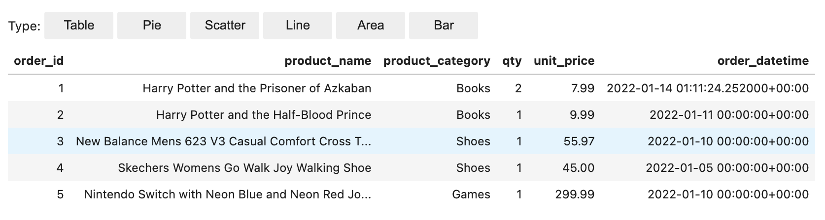
To create visualizations, we use a public dataset on NYC yellow taxis:
In the preceding code block, you read the Parquet file from a public bucket in Amazon S3. The file has headers, and we want Spark to infer the schema. You then use a Spark dataframe to group and count specific columns from taxi_df:
Use %%display magic to view the result in table format:

You can also quickly visualize your data with five types of charts. You can choose the display type and the chart will change accordingly. In the following screenshot, we use a bar chart to visualize our data.

Interact with EMR Serverless using Spark SQL
You can interact with tables in the AWS Glue Data Catalog using Spark SQL on EMR Serverless. In the sample notebook, we show how you can transform data using a Spark dataframe.
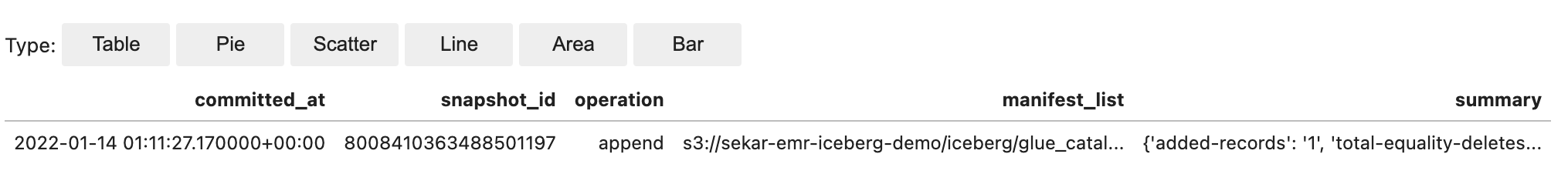
First, create a new temporary view called taxis. This allows you to use Spark SQL to select data from this view. Then create a taxi dataframe for further processing:

In each cell in your EMR Studio notebook, you can expand Spark Job Progress to view the various stages of the job submitted to EMR Serverless while running this specific cell. You can see the time taken to complete each stage. In the following example, stage 14 of the job has 12 completed tasks. In addition, if there is any failure, you can see the logs, making troubleshooting a seamless experience. We discuss this more in the next section.
![Job[14]: showString at NativeMethodAccessorImpl.java:0 and Job[15]: showString at NativeMethodAccessorImpl.java:0](https://d2908q01vomqb2.cloudfront.net/b6692ea5df920cad691c20319a6fffd7a4a766b8/2024/04/05/BDB-3979-image025.png)
Use the following code to visualize the processed dataframe using the matplotlib package. You use the maptplotlib library to plot the dropoff location and the total amount as a bar chart.

Diagnose interactive applications
You can get the session information for your Livy endpoint using the %%info Sparkmagic. This gives you links to access the Spark UI as well as the driver log right in your notebook.

The following screenshot is a driver log snippet for our application, which we opened via the link in our notebook.

Similarly, you can choose the link below Spark UI to open the UI. The following screenshot shows the Executors tab, which provides access to the driver and executor logs.

The following screenshot shows stage 14, which corresponds to the Spark SQL step we saw earlier in which we calculated the location wise sum of total taxi collections, which had been broken down into 12 tasks. Through the Spark UI, the interactive application provides fine-grained task-level status, I/O, and shuffle details, as well as links to corresponding logs for each task for this stage right from your notebook, enabling a seamless troubleshooting experience.

Clean up
If you no longer want to keep the resources created in this post, complete the following cleanup steps:
- Delete the EMR Serverless application.
- Delete the EMR Studio and the associated workspaces and notebooks.
- To delete rest of the resources, navigate to CloudFormation console, select the stack, and choose Delete.
All of the resources will be deleted except the S3 bucket, which has its deletion policy set to retain.
Conclusion
The post showed how to run interactive PySpark workloads in EMR Studio using EMR Serverless as the compute. You can also build and monitor Spark applications in an interactive JupyterLab Workspace.
In an upcoming post, we’ll discuss additional capabilities of EMR Serverless Interactive applications, such as:
- Working with resources such as Amazon RDS and Amazon Redshift in your VPC (for example, for JDBC/ODBC connectivity)
- Running transactional workloads using serverless endpoints
If this is your first time exploring EMR Studio, we recommend checking out the Amazon EMR workshops and referring to Create an EMR Studio.
About the Authors
 Sekar Srinivasan is a Principal Specialist Solutions Architect at AWS focused on Data Analytics and AI. Sekar has over 20 years of experience working with data. He is passionate about helping customers build scalable solutions modernizing their architecture and generating insights from their data. In his spare time he likes to work on non-profit projects, focused on underprivileged Children’s education.
 Disha Umarwani is a Sr. Data Architect with Amazon Professional Services within Global Health Care and LifeSciences. She has worked with customers to design, architect and implement Data Strategy at scale. She specializes in architecting Data Mesh architectures for Enterprise platforms.

 Sekar Srinivasan is a Sr. Specialist Solutions Architect at AWS focused on Big Data and Analytics. Sekar has over 20 years of experience working with data. He is passionate about helping customers build scalable solutions modernizing their architecture and generating insights from their data. In his spare time he likes to work on non-profit projects focused on underprivileged Children’s education.
 Chandra Dhandapani is a Senior Solutions Architect at AWS, where he specializes in creating solutions for customers in Analytics, AI/ML, and Databases. He has a lot of experience in building and scaling applications across different industries including Healthcare and Fintech. Outside of work, he is an avid traveler and enjoys sports, reading, and entertainment.
 Amit Kumar Agrawal is a Senior Solutions Architect at AWS, based out of San Francisco Bay Area. He works with large strategic ISV customers to architect cloud solutions that address their business challenges. During his free time he enjoys exploring the outdoors with his family.
 Viral Shah is a Analytics Sales Specialist working with AWS for 5 years helping customers to be successful in their data journey. He has over 20+ years of experience working with enterprise customers and startups, primarily in the data and database space. He loves to travel and spend quality time with his family.


 Prabu Ravichandran is a Senior Data Architect with Amazon Web Services, focussed on Analytics, data Lake architecture and implementation. He helps customers architect and build scalable and robust solutions using AWS services. In his free time, Prabu enjoys traveling and spending time with family.