Hello, Calgary I am happy to announce that we will be opening an AWS region in Calgary, Canada in late 2023 or early 2024. This three-AZ region will reduce latency for end-users in Western Canada and will also support the development of advanced, distributed solutions that span multiple AWS regions. It will also provide additional flexibility for AWS customers that need to store and process data within Canada’s borders.
As part of our commitment to running our business in the most environmentally friendly way possible, we are also investing in renewable energy projects in Canada. We currently have two projects underway, both in Alberta: an 80 MW solar farm (announced in April 2021) and a 375 MW solar farm (announced in June 2021). Together, these projects will contribute more than one million MWh to the power grid when they come online in 2022.
This region is part of a planned investment of CAD $4.3 billion over the next 15 years, including data center construction, ongoing utilities and facilities costs, and purchases of goods & services from regional businesses. Our Economic Impact Study (EIS) estimates that the spending on infrastructure and construction over the next 15 years will increase Canada’s GDP by about CAD $4.9 billion, along with direct and indirect economic benefits including nearly 1,000 new full-time equivalent jobs in Canada.
And Then There Were Nine With this announcement we now have a total of nine regions (Australia, Canada, India, Indonesia, Israel, New Zealand, Spain, Switzerland, and the United Arab Emirates) in the works. As always, you can find the full list of operational and planned regions on the AWS Global Infrastructure page.
Bonjour Calgary Je suis heureux d’annoncer que nous allons ouvrir une Région AWS à Calgary, au Canada, à la fin de 2023 ou au début de 2024. Cette Région à trois ZD réduira la latence pour les utilisateurs finaux de l’Ouest canadien et permettra aussi de soutenir le développement de solutions avancées et distribuées couvrant plusieurs Régions AWS. De plus, elle fournira une flexibilité supplémentaire aux clients d’AWS ayant besoin de stocker et traiter des données à l’intérieur des frontières canadiennes.
Dans le cadre de notre engagement à gérer notre entreprise de la manière la plus respectueuse de l’environnement possible, nous investissons également dans des projets d’énergie renouvelable au Canada. Nous avons actuellement deux projets en cours, tous deux situés en Alberta : une ferme solaire de 80 MW (annoncée en avril 2021) et une ferme solaire de 375 MW (annoncée en juin 2021). Lorsqu’ils seront opérationnels en 2022, ces projets apporteront conjointement plus de 1 million de MWh au réseau électrique.
Cette Région fait partie d’un investissement prévu de 4,3 milliards de dollars CAD au cours des 15 prochaines années, comprenant la construction de centres de données, les dépenses opérationnelles liées aux services publics et aux installations, ainsi que les achats de biens et de services auprès d’entreprises régionales. Notre étude d’impact économique (EIE) estime que les dépenses en matière d’infrastructure et de construction au cours des 15 prochaines années augmenteront le PIB du Canada d’environ 4,9 milliards de dollars CAD, en plus des retombées économiques directes et indirectes, dont près de 1 000 nouveaux emplois équivalents temps plein au Canada.
Et en voilà une neuvième Avec cette annonce, nous avons maintenant un total de neuf Régions en cours de réalisation (Australie, Canada, Inde, Indonésie, Israël, Nouvelle-Zélande, Espagne, Suisse et les Émirats arabes unis). Comme toujours, vous trouverez la liste complète des Régions opérationnelles et planifiées en consultant la page de l’infrastructure mondiale d’AWS.
The x86 instruction set is large, but that doesn’t mean it can’t get bigger
yet. Upcoming Intel processors will feature a new set of instructions
under the name of “Advanced Matrix Extensions” (AMX) that can be used to
operate on matrix data. After a somewhat bumpy development
process, support for AMX has found its way into the upcoming 5.16 kernel.
Using it will, naturally, require some changes by application developers.
Quantum computers are a boon and a bane. Originally conceived by Manin and Feyman to simulate nature efficiently, large-scale quantum computers will speed-up innovation in material sciences by orders of magnitude. Consider the technical advances enabled by the discovery of new materials (with bronze, iron, steel and silicon each ascribed their own age!); quantum computers could help to unlock the next age of innovation. Unfortunately, they will also break the majority of the cryptography that’s currently used in TLS to protect our web browsing. They fall in two categories:
Digital signatures, such as RSA, which ensure you’re talking to the right server.
Key exchanges, such as Diffie–Hellman, which are used to agree on encryption keys.
A moderately-sized stable quantum computer will easily break the signatures and key exchanges currently used in TLS using Shor’s algorithm. Luckily this can be fixed: over the last two decades, there has been great progress in so-called post-quantum cryptography. “Post quantum”, abbreviated PQ, means secure against quantum computers. Five years ago, the standards institute NIST started a public process to standardise post-quantum signature schemes and key exchanges. The outcome is expected to be announced early 2022.
At Cloudflare, we’re not just following this process closely, but are also testing the real-world performance of PQ cryptography. In our 2019 experiment with Google, we saw that we can switch to a PQ key exchange with little performance impact. Among the NIST finalists, there are many with even better performance. This is good news, as we would like to switch to PQ key exchanges as soon as possible — indeed, an attacker could intercept sensitive data today, then keep and decrypt it years into the future using a quantum computer.
Why worry about PQ signatures today
One would think we can take it easy with signatures for TLS: we only need to have them replaced before a large quantum computer is built. The situation, however, is more complicated.
The lead time to change signatures is higher. Not only do we need to change the browsers and servers, we also need to change certificate authorities (CAs) and everyone’s certificate management.
TLS is addicted to small and fast signatures. For this page that you’re viewing we sent six signatures: two in the certificate chain; one handshake signature; one OCSP staple and finally two SCTs used for certificate transparency.
PQ signature schemes have wildly varying performance trade-offs and quirks (as we’ll see below) which stack up quickly with six signatures, which all have slightly different requirements.
One might ask: can’t we be clever and get rid of some of these signatures? We think so! For instance, we can replace the handshake signature with a smaller key exchange or suppress intermediate certificates. Such fundamental changes take years to be adopted. That is why we are also investigating the performance of plain TLS with drop-inPQ signatures.
So, what are our options?
The zoo of PQ signatures
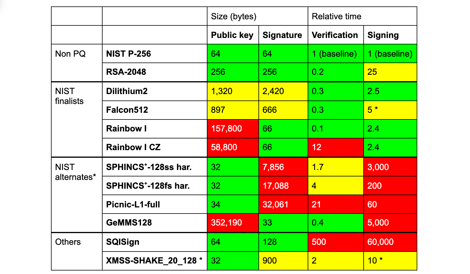
The three finalists of the NIST competition are Dilithium, Falcon and Rainbow. In the table below we compare them against RSA and ECDSA, both of which are in common use today, and a selection of other PQ schemes that might see standardisation in the future.
(* There are many caveats to this table. We compare instances of PQC security level 1. Signing and verification times vary considerably by hardware platform and implementation constraints. They should be taken as a rough indication only. The signing time of Falcon512 is discussed later on. We do not list all relevant variants of the NIST alternates or promising schemes. This instance of XMSS can only sign a million messages, is stateful, requires quite a bit of storage for quick signing, is not standardised and thus far from a drop-in replacement. Rainbow has one other variant, which has smaller private keys.)
None of these PQ signatures are a clear-cut drop-in replacement. To start, all have (much) larger signatures, except for Rainbow, GeMMS and SQISign. Rainbow and GeMMS have huge public keys and SQISign is very slow.
TLS signatures
To confuse matters even more, the signatures within TLS are not all the same:
Online. Only the handshake signature is created with every incoming TLS connection, and so signing needs to be fast. Dilithium fits this role well.
Offline. All other signatures are made months/years in advance, and so signing time is not that important. This group splits in two:
With a public key. The certificate chain includes signatures and their public keys. Here Falcon seems most suited.
Without a public key. The remaining three (SCTs and OCSP staple) are just signatures. For these, Rainbow seems optimal, as its large public keys are not transmitted.
Using Dilithium, Falcon, and Rainbow, together, allows optimization for both speed and size simultaneously, which seems like a great idea. However, combining different signatures at the same time has disadvantages:
A security issue in the design or implementation of one of the signatures compromises the whole.
Clients need to implement multiple cryptographic algorithms, in this case three of them, which is troublesome for smaller devices — especially if separate hardware support is needed for each of them.
So do we really need to eke out every byte and every cycle of performance? Or can we stick to a single signature scheme for simplicity and security?
Can we pick just one?
If we stick to one signature scheme, looking just at the numbers, Falcon512 seems like a reasonable option. It needs 5KB of extra space (compared to a classical handshake), about the same as the Dilithium–Falcon–Rainbow chimera of before. Unfortunately Falcon comes with a caveat: creating signatures efficiently requires constant-time 64-bit floating point arithmetic. Without it, signing is 20x slower. But speed alone is not enough; it has to run inconstant time. Without that, one can slowly learn the secret key by measuring the time it takes to create a signature.
Although PCs typically have a sufficiently constant-time floating-point unit, many smaller devices do not. Thus, Falcon seems ill-suited for general purpose online signatures.
What about Dilithium2? It needs 17KB extra — let’s find out if that makes a big difference.
Evidence by Experiment
All the different variables and constraints clearly complicate an already challenging puzzle. The best thing is to just try the options. Over the last few years several interesting papers have appeared studying the various options, such as SKD20, PST20, SKD21 and PKNLN22. These are great starts, but don’t provide a complete picture:
SCTs and OCSP staples have yet to be considered. Leaving half (three) of the signatures out changes the results significantly.
The networks tested or emulated offer insights, but are far from representative of real-world conditions. All tests were conducted between two datacenters (which does not include real-world last-mile conditions such as Wi-Fi or spotty mobile connections); or a network was simulated with unrealistic packet loss rates.
Here, Cloudflare can contribute. One of the things we like to do is to put new ideas in the community to the test on a global scale.
In this case we’re just taking a first step. Setting up a real-world experiment with a modified browser is quite involved, especially when we consider the many possible variations. Instead, as a first step, we decided first to investigate the most striking variable, the size, and try to answer the question:
How do larger signatures affect the TLS handshake?
There are two parts to this: how fast are they, and, more importantly, do they work at all?
Experimental setup
We need some way to emulate bigger signatures without having to modify the clients. We considered several options. The first idea we had was to pad a valid certificate with a dummy extension. That would require a custom certificate for each size to test, which is cumbersome. Then we considered responding with a dummy ServerHello extension. This is, however, not allowed by TLS 1.2 without a corresponding ClientHello extension. In the end, we went for adding dummy certificates.
Dummy certificates
These dummy certificates are 1kB self-signed invalid certificates that have nothing to do with the certificate chain. To vary the size to test, we simply add more copies. Adding unrelated certificates to the certificate chain is a common misconfiguration and clients have learnt to ignore them. In fact, TLS 1.3 stipulates that these (in rfc-speak) SHOULD be ignored by the client. Testing out hundreds of browsers, we saw no issues.
Standards and reality don’t always agree: when inserting dummy certificates on actual traffic, we saw issues with a small, but not insignificant number of clients. We don’t want to ruin anyone’s connection, and so we decided to use separate connections for this purpose.
Using challenge pages to launch probes
So what did we actually do? On a small percentage of the challenge pages (those with the CAPTCHA), we pick a number n and a random key and send this key in two separate background requests to:
0.tls-size-experiment-c.cloudflareresearch.com
[n].tls-size-experiment-1.cloudflareresearch.com
The first, the control, is a normal webpage that stores the TLS handshake time under the key that’s been sent. The real action happens at the second, the live, which adds the n dummy certificates to its chain. The live also stores handshake time under the given key. We could call it “experimental” instead of “live”, but the benign control connection is also an important part of the experiment. Indeed, it allows us to see if live connections are missing. These endpoints were a breeze to write using Cloudflare Workers and KV.
How much dummy data to test?
Before launching the experiment, we tested several libraries and browsers on the live endpoint to see whether they would error due to the dummy certificates. None rejected a single certificate, but how far can we go? TLS 1.3 theoretically allows a certificate chain of 16MB, but in practice many clients reject a much shorter chain. OpenSSL, for instance, rejects one of 102kB. The most stingy we found is Go’s TLS client, which rejects a handshake larger than 64kB. Because of this, we tested with between 1 and 59 dummy certificates.
Intermezzo: TCP’s congestion window
So, what did we find? The graphs are in the next section, have a peek! Before diving right in, we would like to explain a crucial concept, the TCP congestion window, that helps us read the results.
Data sent over the Internet is broken down in packets of around 1.4kB that traverse many routers to reach their destination. Sometimes a router has more incoming packets than it can handle and it has to drop them — this is called congestion. To avoid causing congestion, TCP initially sends just a few packets (typically ten, so ~14kB). Then, with every acknowledgement received in return, the TCP sender will very quickly ramp up the number of packets that it keeps in flight. This number is called the congestion window (cwnd). When it gets too high, congestion occurs, packets are dropped and in response the sender backs off by dialing down the congestion window. Any dropped packet is seen as a sign of congestion by TCP. For this reason, Wi-Fi has its own retransmission mechanism transparent to TCP.
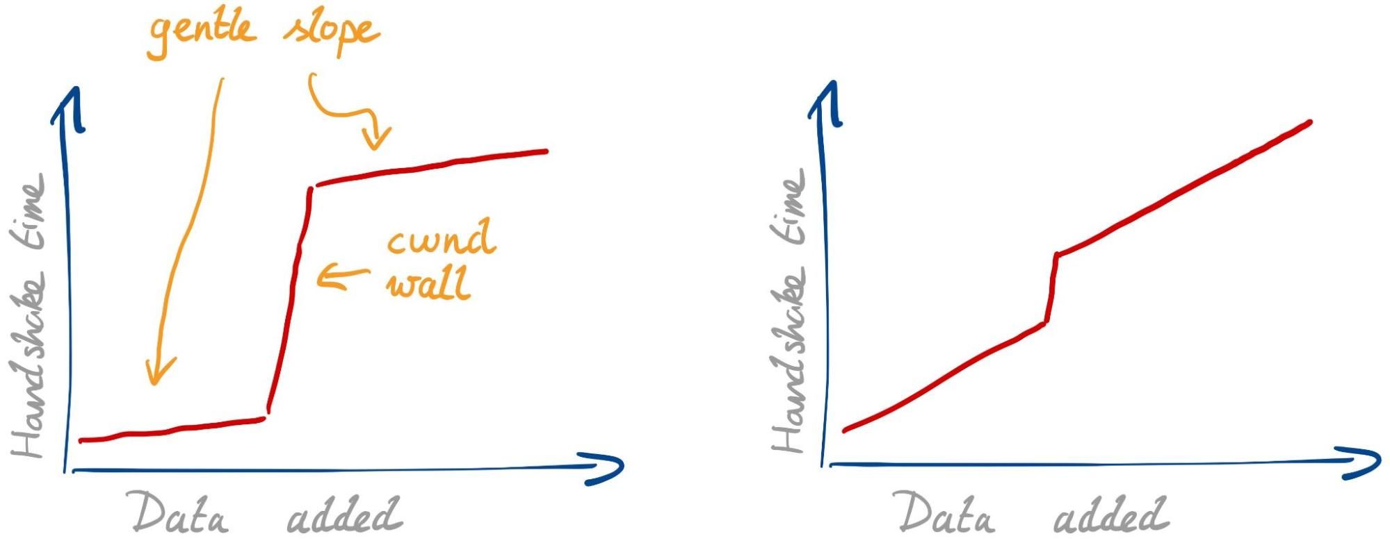
Considering all this, we would expect to see two effects with larger signatures:
Gentle slope. Every single packet needs some extra time to transmit, due to limited bandwidth and possible physical-layer retransmissions. This slope isn’t so gentle if your internet connection is slow or spotty.
cwnd wall. Once we fill the congestion window, we have to wait for a whole roundtrip before we can continue. This effect is stronger if the roundtrip time (RTT) is higher.
The strength of the two effects can differ. With a fast connection and high RTT we expect to see the graph below on the left. With a slow connection and low RTT, we expect the one on the right.
There might be other unknown effects. The best thing is to have a look.
In PQ research, the second effect has gained the most attention. The larger signatures simply do not fit in the initial congestion windows used today. A common suggestion in response has been to simply increase the initial congestion window to accommodate the larger signatures. This is far from a simplechange to make globally, and we have to understand if this solves the problem to begin with.
Results
Over 24 days we’ve received 964,499 live connections from 454,218 different truncated IPs (to 24 bits, “/24”, for IPv4 and 48 bits for IPv6) and 11,239 different ASNs. First, let’s check how many clients had trouble with the bigger handshakes.
Can clients handle the larger handshakes?
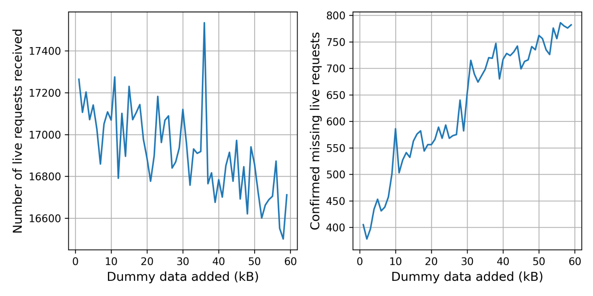
The control connection was missing for 2.4% of the live connections. This is not alarming: we expect some connections to be missing for harmless reasons, such as the user browsing away from the challenge page. There are, however, significantly more live connections without control connection at 3.6%.
In the graph below on the left we break the number of received live connections down by the number of dummy certificates added. Because we pick the number of certificates randomly, the graph is noisy. To get a clearer picture, we started storing the number of certificates added in the corresponding control request, which gives us the graph on the right. The bumps at 10kB and 30kB suggest that there are clients or middleboxes that cannot handle these handshake sizes.
Handshake times with larger signatures
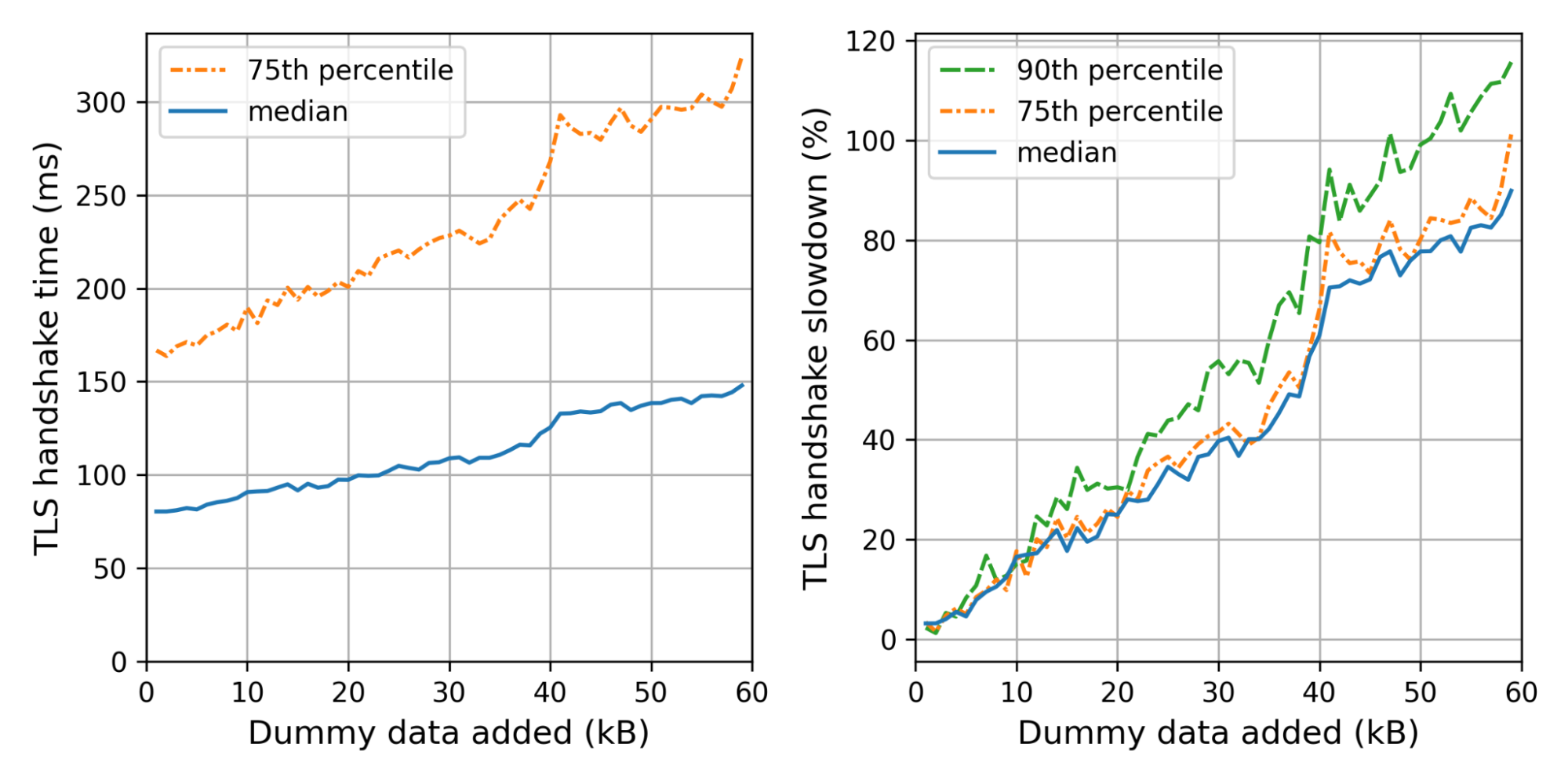
What is the effect on the handshake time? The graph on the left shows the weighted median and 75th percentile TLS handshake times for different amounts of dummy data added. We use the weight so that every truncated IP contributes equally. On the right we show the slowdowns for each size, relative to the handshake time of the control connection.
We can see the not-so-gentle slope until 40kB, where we hit a littlewall that corresponds to Cloudflare’s default initial congestion window of 30 packets.
Adding 35kB fits within our initial congestion window. Nonetheless, the median handshake with 35kB extra is 40% slower. The slowest 10% are even worse off, taking 60% as much time. Thus even though we stay within the congestion window, the added data is not for free at all.
We can now translate these insights back to concrete PQ signatures. For example, using Dilithium2 as a drop-in replacement, we need around 17kB extra. That also fits within our initial congestion window with a median slowdown of 20%, which gets worse for the tail-end of users. For the normal initial congestion window of ten, we expect the slowdown to be much worse — around 60–80%.
There are several caveats to point out:
These experiments used an initial congestion window of 30 packets instead of ten. With a smaller initial congestion window of ten, which is the default for most systems, we would expect the wall to move from 40kB to around 10kB.
Because of our presence all across the world, our RTTs are fairly low. Thus the effect of the cwnd wall is smaller for us.
Challenge pages are served, by design, to those clients that we expect to be bots. This adds a significant bias because bots are generally hosted at well-connected providers, and so are closer than users.
HTTP/3 was not supported by the server we used for the endpoint. Support for IPv6 was only added ten days into the experiment and accounts for 10.9% of the measurements.
Actual TLS handshakes differ in size much more than tested in this setup due to differences in certificate sizes and extensions and other factors.
What have we learned?
The TLS handshake is just one step (~5–20%) in a long chain required to show you a webpage. Casually browsing, it would be hard to notice a TLS handshake that’s 60% slower. But such differences add up. To make a website really fast, you need many seemingly insignificant speedups. Browser developers take this seriously: only in exceptional cases does Chrome allow a change that slows down any microbenchmark by even a percent.
Because of the many parties and complexities involved, we should avoid waiting too long to adopt post-quantum signatures in TLS. That’s a hard sell if it comes at the price of a double-digit slowdown, not least to content servers but also to browser vendors and clients.
A timely adoption of PQ signatures on the web would be great. Our evidence so far suggests that this will be easiest, if six signatures and two public keys would fit in 9kB.
We will continue our efforts to help build a post-quantum secure Internet. To follow along, keep an eye on this blog or have a look at research.cloudflare.com.
Bas Westerbaan is co-submitter of the SPHINCS+ signature scheme.
Security updates have been issued by Debian (containerd, redis, and sqlalchemy), Fedora (kernel, radeontop, rpki-client, and webkit2gtk3), openSUSE (java-1_8_0-openj9, libvirt, mailman, transfig, and webkit2gtk3), Oracle (thunderbird), SUSE (libvirt), and Ubuntu (icu).
Tina Peters, the election clerk in Mesa County (Colorado) went rogue and dumped disk images of an election computer on the Internet. They are available on the Internet via BitTorrent [Mesa1][Mesa2], The Colorado Secretary of State is now suing her over the incident.
The lawsuit describes the facts of the case, how she entered the building with an accomplice on Sunday, May 23, 2021. I thought I’d do some forensics on the image to get more details.
Specifically, I see from the Mesa1 image that she logged on at 4:24pm and was done acquiring the image by 4:30pm, in and (presumably) out in under 7 minutes.
In this blogpost, I go into more detail about how to get that information.
The image
To download the Mesa1 image, you need a program that can access BitTorrent, such as the Brave web browser or a BitTorrent client like qBittorrent. Either click on the “magnet” link or copy/paste into the program you’ll use to download. It takes a minute to gather all the “metadata” associated with the link, but it’ll soon start the download:
What you get is file named EMSSERVER.E01. This is a container file that contains both the raw disk image as well as some forensics metadata, like the date it was collected, the forensics investigator, and so on. This container is in the well-known “EnCase Expert Witness” format. EnCase is a commercial product, but its container format is a quasi-standard in the industry.
Some freeware utilities you can use to open this container and view the disk include “FTK Imager”, “Autopsy”, and on the Linux command line, “ewf-tools”.
However you access the E01 file, what you most want to look at is the Windows operating-system logs. These are located in the directory C:\Windows\system32\winevtx. The standard Windows “Event Viewer” application can load these log files to help you view them.
When inserting a USB drive to create the disk image, these event files will be updated and written to that disk before the image was taken. Thus, we can see in the event files all the events that happen right before the disk image happens.
Disk image acquisition
Here’s what the event logs on the Mesa1 image tells us about the acquisition of the disk image itself.
The person taking the disk image logged in at 4:24:16pm, directly to the console (not remotely), on their second attempt after first typing an incorrect password. The account used was “emsadmin”. Their NTLM password hash is 9e4ec70af42436e5f0abf0a99e908b7a. This is a “role-based” account rather than an individual’s account, but I think Tina Peters is the person responsible for the “emsadmin” roll.
Then, at 4:26:10pm, they connected via USB a Western Digital “easystore™” portable drive that holds 5-terabytes. This was mounted as the F: drive.
The program “Access Data FTK Imager 4.2.0.13” was run from the USB drive (F:\FTK Imager\FTK Imager.exe) in order to image the system. The image was taken around 4:30pm, local Mountain Time (10:30pm GMT).
It’s impossible to say from this image what happened after it was taken. Presumably, they immediately hit “eject” on the drive, logged off, and disconnected the hard drive. Thus from beginning to end, it took about 7 minutes to take the image once they sat down at the computer.
Dominion Voting Systems
The disk image is that of a an “EMS Server” part of the Dominion Voting Suite. This is a server on an air-gapped network (not connected to any other network) within the count offices.
Most manuals for Colorado are online, though some bits and pieces are missing, and can be found in documents posted to other state’s websites (though each state does things a little different, so such cross referencing can’t be completely trusted).
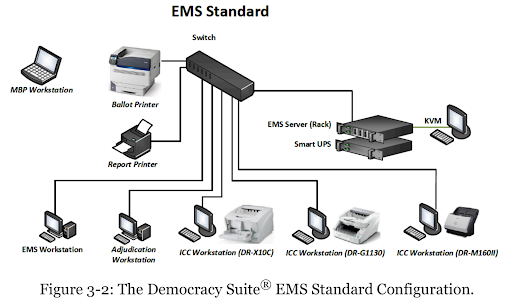
The locked room with an air-gapped network you see in the Mesa County office appears to look like the following, an “EMS Standard” configuration (EMS stands for Election Management System).
This small network is “air gapped”, meaning there is no connection from this network to any other network in the building, nor out to the Internet. By looking at the logs from the Mesa1 image, we can see what this network looks like:
The EMS Server is named “EMSERVER” with IP address 192.168.100.10 and MAC address 44-A8-42-30-01-5D. The hard drive matches Dominion’s specs: a 1-terabyte boot drive (C:) and a 2-terabyte data drive (D:) that is shared with the rest of the network as \\EMSERVER\NAS. This also acts as the network’s DHCP and DNS server.
At least one network printer, model Dell E310dw.
Two EMS Workstations (EMSCLIENT01 and EMSCLIENT02). This is where users spend most of their time, before an election to create the ballots, and after all the ballots have been counted to construct the final tally.
Four ImageCast Central (ICC) (ICC01 – ICC04) scanners, for automatically scanning and tabulating ballots.
Two Adjudication Workstations (ADJCLIENT01 and ADJCLIENT03). These are used when the scanners reject ballots, such as when somebody does a write-in candidate, or marks two candidates. Humans need to get involved to make the final judgement on what the ballot actually says.
Note this isn’t the machines you’d expect to see in a precinct when you vote (which would be “ballot marking devices” predominantly). These are the machines in the back office that count the votes and store the official results.
Conclusion
What we see here is that “system logs” can tell us a lot of interesting things about the system. There’s good reason to retain them in the future.
On the other hand, they generally can’t answer the most important question: whether the system was hacked and votes flipped.
Mike Lindell claims to have “Absolute Proof” that Chinese hackers flipped votes throughout the country, including Maricopa County. If so, this would’ve been the system that the Chinese hackers would’ve hacked. Yet, in the system image, there is no evidence of this. By this, I mean the Mesa1 image, the one from before the system logs were deleted (obviously, there would be nothing in the Mesa2 image).
This lack of hacking evidence in the logs isn’t proof that it didn’t happen, though. The fact is, the logs aren’t comprehensive enough to record most hacks, and the hackers could’ve deleted the logs anyway. That’s why system logs aren’t considered “election records” and that laws don’t mandate keeping them: they could have some utility, as I’ve shown above, but they really wouldn’t show the things that we most want to know.
Applying various transformations to images at scale is an easily parallelized and scaled task. As a Computer Vision research team at Amazon, we occasionally find that the amount of image data we are dealing with can’t be effectively computed on a single machine, but also isn’t large enough to justify running a large and potentially costly AWS Elastic Map Reduce (EMR) job. This is when we can utilize AWS Batch as our main computing environment, as well as Cloud Development Kit (CDK) to provision the necessary infrastructure in order to solve our task.
In Computer Vision, we often need to represent images in a more concise and uniform way. Working with standard image files would be challenging, as they can vary in resolution or are otherwise too large in terms of dimensionality to be provided directly to our models. For that reason, the common practice for deep learning approaches is to translate high-dimensional information representations, such as images, into vectors that encode most (if not all) information present in them — in other words, to create vector embeddings.
This post will demonstrate how we utilize the AWS Batch platform to solve a common task in many Computer Vision projects — calculating vector embeddings from a set of images so as to allow for scaling.
Architecture Overview
Figure 1: High-level architectural diagram explaining the major solution components.
As seen in Figure 1, AWS Batch will pull the docker image containing our code onto provisioned hosts and start the docker containers. Our sample code, referenced in this post, will then read the resources from S3, conduct the vectorization, and write the results as entries in the DynamoDB Table.
In order to run our image vectorization task, we will utilize the following AWS cloud components:
Amazon ECR — Elastic Container Registry is a Docker image repository from which our batch instances will pull the job images;
S3 — Amazon Simple Storage Service will act as our image source from which our batch jobs will read the image;
Amazon DynamoDB — NoSQL database in which we will write the resulting vectors and other metadata;
AWS Lambda — Serverless compute environment which will conduct some pre-processing and, ultimately, trigger the batch job execution; and
AWS Batch — Scalable computing environment powering our models as embarrassingly parallel tasks running as AWS Batch jobs.
To translate an image to a vector, we can utilize a pre-trained model architecture, such as AlexNet, ResNet, VGG, or more recent ones, like ResNeXt and Vision Transformers. These model architectures are available in most of the popular deep learning frameworks, and they can be further modified and extended depending on our project requirements. For this post, we will utilize a pre-trained ResNet18 model from MxNet. We will output an intermediate layer of the model, which will result in a 512 dimensional representation, or, in other words, a 512 dimensional vector embedding.
Deployment using Cloud Development Kit (CDK)
In recent years, the idea of provisioning cloud infrastructure components using popular programming languages was popularized under the term of infrastructure as code (IaC). Instead of writing a file in the YAML/JSON/XML format, which would define every cloud component we want to provision, we might want to define those components trough a popular programming language.
As part of this post, we will demonstrate how easy it is to provision infrastructure on AWS cloud by using Cloud Development Kit (CDK). The CDK code included in the exercise is written in Python and defines all of the relevant exercise components.
Hands-on exercise
1. Deploying the infrastructure with AWS CDK
For this exercise, we have provided a sample batch job project that is available on Github (link). By using that code, you should have every component required to do this exercise, so make sure that you have the source on your machine. The root of your sample project local copy should contain the following files:
batch_job_cdk - CDK stack code of this batch job project
src_batch_job - source code for performing the image vectorization
src_lambda - source code for the lambda function which will trigger the batch job execution
app.py - entry point for the CDK tool
cdk.json - config file specifying the entry point for CDK
requirements.txt - list of python dependencies for CDK
README.md
If you have multiple AWS CLI profiles, utilize the --profile option to specify which profile to use for deployment. Otherwise, simply run cdk deploy and deploy the infrastructure to your AWS account set in step 1.
NOTE: Before deploying, make sure that you are familiar with the restrictions and limitations of the AWS services we are using in this post. For example, if you choose to set an S3 bucket name in the CDK Bucket construct, you must avoid naming conflicts that might cause deployment errors.
The CDK tool will now trigger our docker image build, provision the necessary AWS infrastructure (i.e., S3 Bucket, DynamoDB table, roles and permissions), and, upon completion, upload the docker image to a newly created repository on Amazon Elastic Container Registry (ECR).
2. Upload data to S3
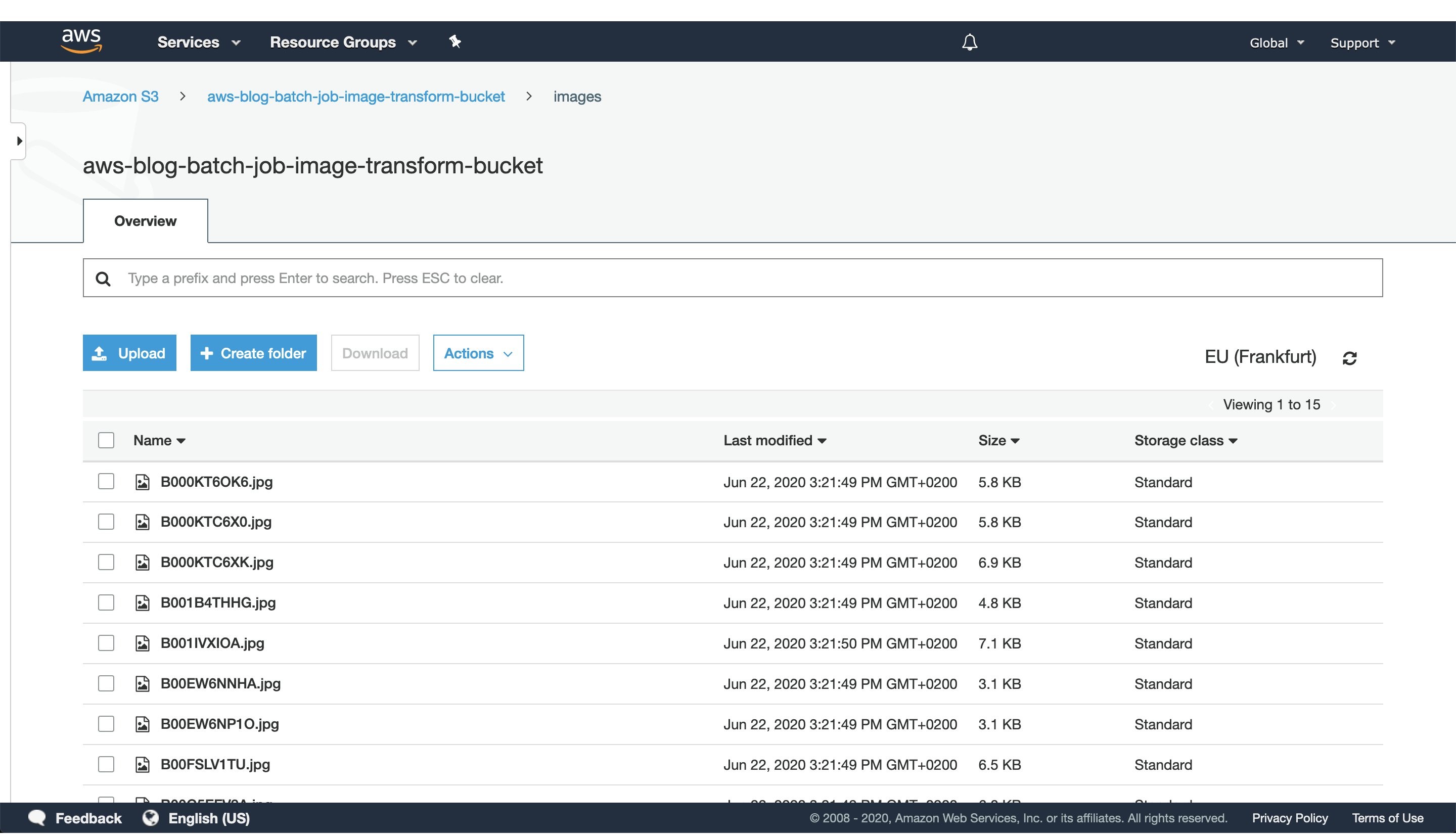
Figure 2: S3 console window with uploaded images to the `images` directory.
After CDK has successfully finished deploying, head to the S3 console screen and upload images you want to process to a path in the S3 bucket. For this exercise, we’ve added every image to the `images` directory, as seen in Figure 2.
For larger datasets, utilize the AWS CLI tool to sync your local directory with the S3 bucket. In that case, consider enabling the ‘Transfer acceleration’ option of your S3 bucket for faster data transfers. However, this will incur an additional fee.
3. Trigger batch job execution
Once CDK has completed provisioning our infrastructure and we’ve uploaded the image data we want to process, open the newly created AWS Lambda in the AWS console screen in order to trigger the batch job execution.
To do this, create a test event with the following JSON body:
{
"Paths": [
    "images"
   ]
}
The JSON body that we provide as input to the AWS Lambda function defines a list of paths to directories in the S3 buckets containing images. Having the ability to dynamically provide paths to directories with images in S3, lets us combine multiple data sources into a single AWS Batch job execution. Furthermore, if we decide in the future to put an API Gateway in front of the Lambda, you could pass every parameter of the batch job with a simple HTTP method call.
In this example, we specified just one path to the `images` directory in the S3 bucket, which we populated with images in the previous step.
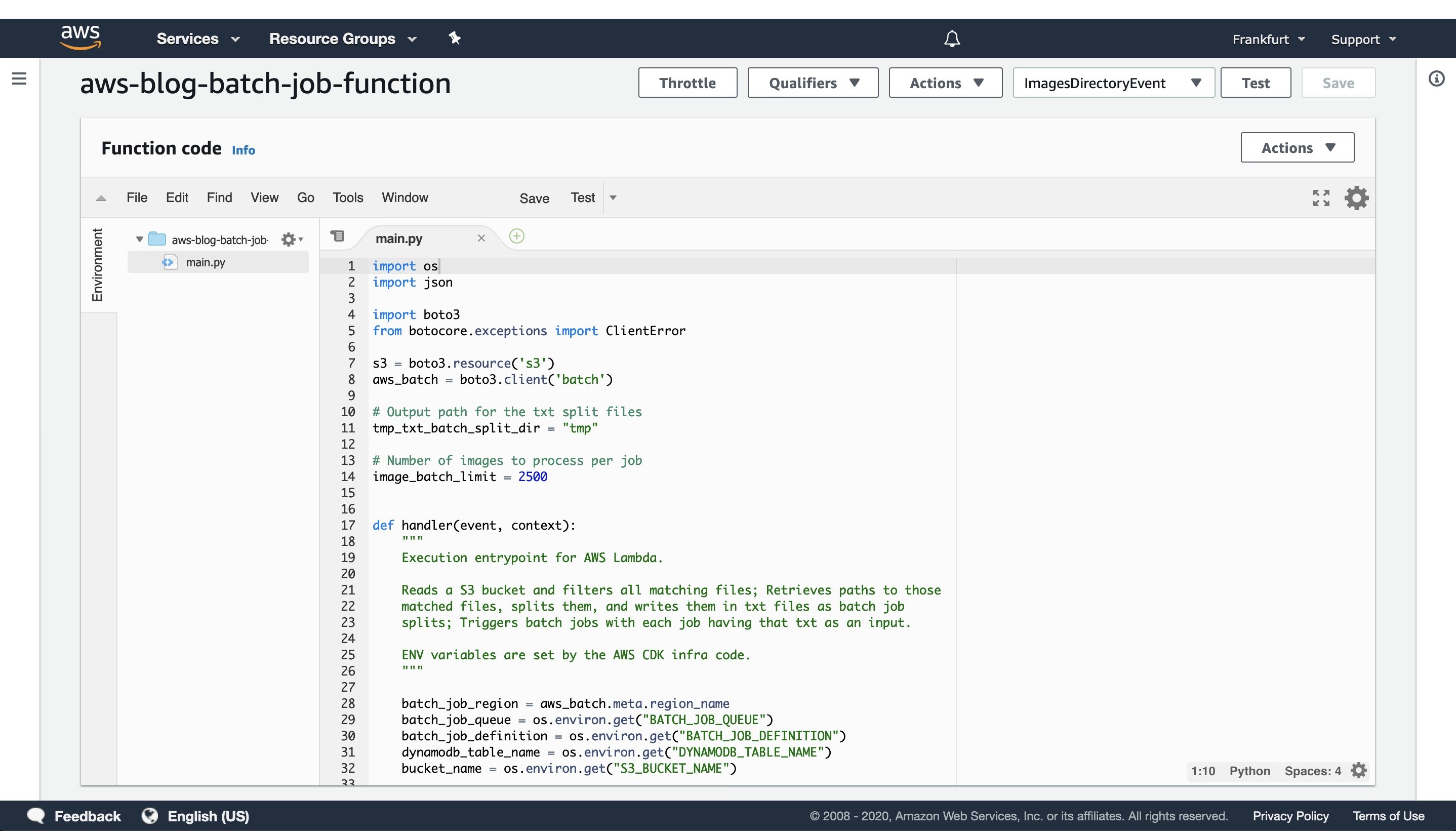
Figure 3: AWS Lambda console screen of the function that triggers batch job execution. Modify the batch size by modifying the `image_batch_limit` variable. The value of this variable will depend on your particular use-case, computation type, image sizes, as well as processing time requirements.
The python code will list every path under the images S3 path, batch them into batches of desired size, and finally save the paths to batches as txt files under tmp S3 path. Each path to a txt files in S3 will be passed as an input to a batch jobs.
Select the newly created event, and then trigger the Lambda function execution. The AWS Lambda function will submit the AWS Batch jobs to the provisioned AWS Batch compute environment.
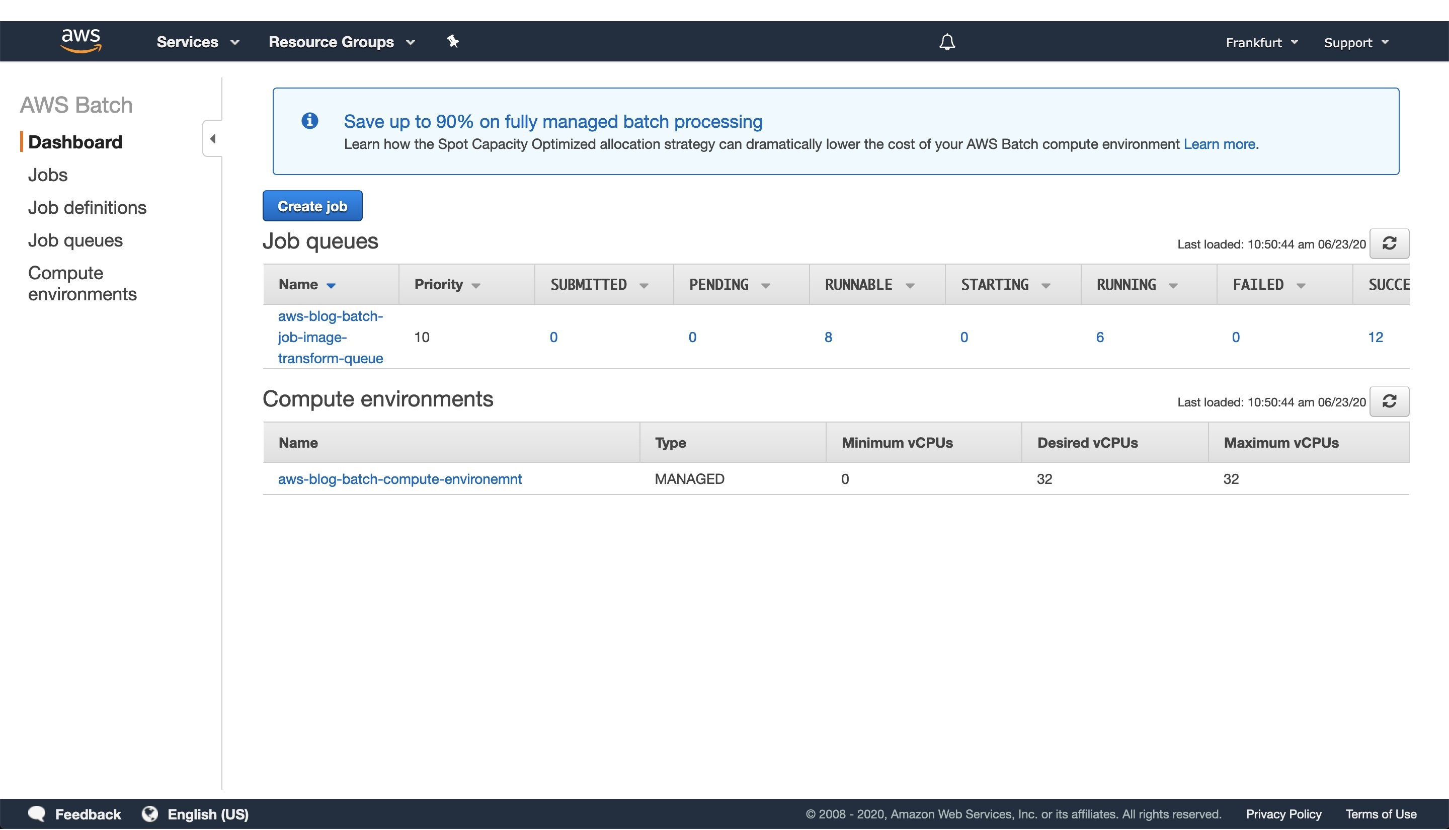
Figure 4: Screenshot of a running AWS Batch job that creates feature vectors from images and stores them to DynamoDB.
Once the AWS Lambda execution finishes its execution, we can monitor the AWS Batch jobs being processed on the AWS console screen, as seen in Figure 4. Wait until every job has finished successfully.
4. View results in DynamoDB
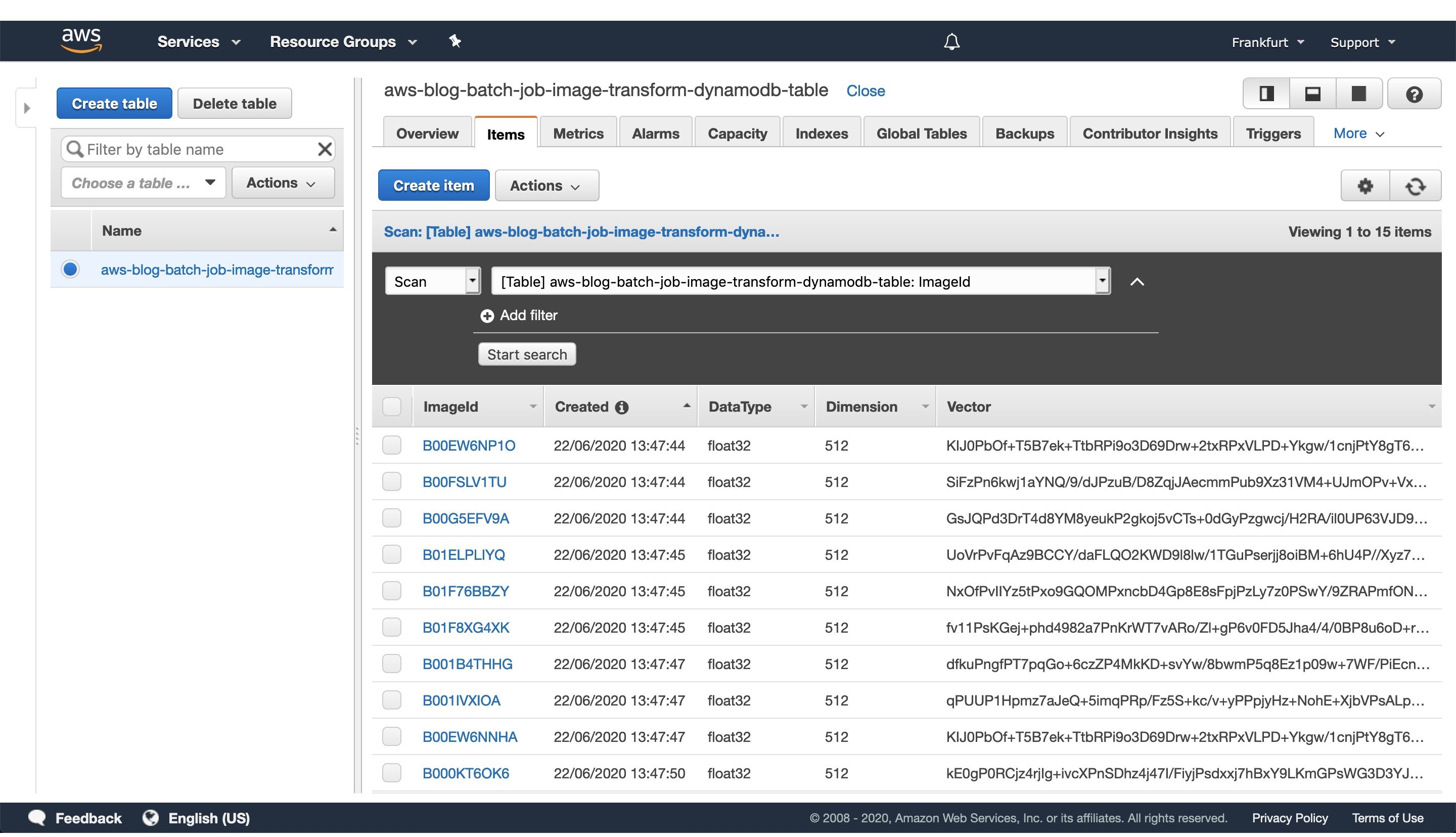
Figure 5: Image vectorization results stored for each image as a entry in the DynamoDB table.
Once every batch job is successfully finished, go to the DynamoDB AWS cloud console and see the feature vectors stored as strings obtained from the numpy tostring method, as well as other data we stored in the table.
When you are ready to access the vectors in one of your projects, utilize the code snippet provided here:
#!/usr/bin/env python3

import numpy as np
import boto3

def vector_from(item):
    '''
    Parameters
    ----------
    item : DynamoDB response item object
    '''
    vector = np.frombuffer(item['Vector'].value, dtype=item['DataType'])
    assert len(vector) == item['Dimension']
    return vector

def vectors_from_dydb(dynamodb, table_name, image_ids):
    '''
    Parameters
    ----------
    dynamodb : DynamoDB client
    table_name : Name of the DynamoDB table
    image_ids : List of id's to query the DynamoDB table for
    '''

    response = dynamodb.batch_get_item(
        RequestItems={table_name: {'Keys': [{'ImageId': val} for val in image_ids]}},
        ReturnConsumedCapacity='TOTAL'
    )

    query_vectors =  [vector_from(item) for item in response['Responses'][table_name]]
    query_image_ids =  [item['ImageId'] for item in response['Responses'][table_name]]

    return zip(query_vectors, query_image_ids)

def process_entry(vector, image_id):
    '''
    NOTE - Add your code here.
    '''
    pass

def main():
    '''
    Reads vectors from the batch job DynamoDB table containing the vectorization results.
    '''
    dynamodb = boto3.resource('dynamodb', region_name='eu-central-1')
    table_name = 'aws-blog-batch-job-image-transform-dynamodb-table'

    image_ids = ['B000KT6OK6', 'B000KTC6X0', 'B000KTC6XK', 'B001B4THHG']

    for vector, image_id in vectors_from_dydb(dynamodb, table_name, image_ids):
        process_entry(vector, image_id)

if __name__ == "__main__":
    main()
This code snippet will utilize the boto3 client to access the results stored in the DynamoDB table. Make sure to update the code variables, as well as to modify this implementation to one that fits your use-case.
5. Tear down the infrastructure using CDK
To finish off the exercise, we will tear down the infrastructure that we have provisioned. Since we are using CDK, this is very simple — go to the project root directory and run:
cdk destroy
After a confirmation prompt, the infrastructure tear-down should be underway. If you want to follow the process in more detail, then go to the CloudFormation console view and monitor the process from there.
NOTE: The S3 Bucket, ECR image, and DynamoDB table resource will not be deleted, since the current CDK code defaults to RETAIN behavior in order to prevent the deletion of data we stored there. Once you are sure that you don’t need them, remove those remaining resources manually or modify the CDK code for desired behavior.
Conclusion
In this post we solved an embarrassingly parallel job of creating vector embeddings from images using AWS batch. We provisioned the infrastructure using Python CDK, uploaded sample images, submitted AWS batch job for execution, read the results from the DynamoDB table, and, finally, destroyed the AWS cloud resources we’ve provisioned at the beginning.
AWS Batch serves as a good compute environment for various jobs. For this one in particular, we can scale the processing to more compute resources with minimal or no modifications to our deep learning models and supporting code. On the other hand, it lets us potentially reduce costs by utilizing smaller compute resources and longer execution times.
The code serves as a good point for beginning to experiment more with AWS batch in a Deep Leaning/Machine Learning setup. You could extend it to utilize EC2 instances with GPUs instead of CPUs, utilize Spot instances instead of on-demand ones, utilize AWS Step Functions to automate process orchestration, utilize Amazon SQS as a mechanism to distribute the workload, as well as move the lambda job submission to another compute resource, or pretty much tailor your project for anything else you might need AWS Batch to do.
And that brings us to the conclusion of this post. Thanks for reading, and feel free to leave a comment below if you have any questions. Also, if you enjoyed reading this post, make sure to share it with your friends and colleagues!
About the author
The collective thoughts of the interwebz
Manage Consent
To provide the best experiences, we use technologies like cookies to store and/or access device information. Consenting to these technologies will allow us to process data such as browsing behavior or unique IDs on this site. Not consenting or withdrawing consent, may adversely affect certain features and functions.
Functional
Always active
The technical storage or access is strictly necessary for the legitimate purpose of enabling the use of a specific service explicitly requested by the subscriber or user, or for the sole purpose of carrying out the transmission of a communication over an electronic communications network.
Preferences
The technical storage or access is necessary for the legitimate purpose of storing preferences that are not requested by the subscriber or user.
Statistics
The technical storage or access that is used exclusively for statistical purposes.The technical storage or access that is used exclusively for anonymous statistical purposes. Without a subpoena, voluntary compliance on the part of your Internet Service Provider, or additional records from a third party, information stored or retrieved for this purpose alone cannot usually be used to identify you.
Marketing
The technical storage or access is required to create user profiles to send advertising, or to track the user on a website or across several websites for similar marketing purposes.
 This region is part of a planned investment of CAD $4.3 billion over the next 15 years, including data center construction, ongoing utilities and facilities costs, and purchases of goods & services from regional businesses. Our Economic Impact Study (EIS) estimates that the spending on infrastructure and construction over the next 15 years will increase Canada’s GDP by about CAD $4.9 billion, along with direct and indirect economic benefits including nearly 1,000 new full-time equivalent jobs in Canada.