Post Syndicated from Explosm.net original https://explosm.net/comics/sperm
New Cyanide and Happiness Comic
Post Syndicated from Explosm.net original https://explosm.net/comics/sperm
New Cyanide and Happiness Comic
Post Syndicated from original https://lwn.net/Articles/934459/
The fifth conference on Power
Management and Scheduling in the Linux Kernel (abbreviated “OSPM”) was
held on April 17 to 19 in Ancona, Italy. LWN was not there,
unfortunately, but the attendees of the event have gotten together to write
up summaries of the discussions that took place and LWN has the privilege
of being able to publish them. Reports from the second day of the event
appear below.
Post Syndicated from original https://lwn.net/Articles/934939/
Security updates have been issued by Debian (chromium, openjdk-17, and wireshark), Fedora (iniparser, mariadb, mingw-glib2, perl-HTML-StripScripts, php, python3.7, and syncthing), Oracle (.NET 6.0, c-ares, kernel, nodejs, and python3.9), Slackware (libX11), SUSE (amazon-ssm-agent and chromium), and Ubuntu (gsasl, libx11, and sssd).
Post Syndicated from LGR original https://www.youtube.com/watch?v=6bODiZ5bP84
Post Syndicated from original https://lwn.net/Articles/934883/
The developers working on improving the speed of the CPython interpreter
have posted
a plan describing their objectives for the Python 3.13 release. The
biggest piece appears to be the tier-2
optimizer, which will optimize larger chunks of Python code:
“https://github.com/faster-cpython/ideas/issues/557
“.
Post Syndicated from The History Guy: History Deserves to Be Remembered original https://www.youtube.com/watch?v=u-E4FyPxPmc
Post Syndicated from Анета Василева original https://www.toest.bg/zatvorut-na-21-vek/

Този текст е базиран на проучванията, направени заедно с Дарина Банова през есента на 2022 г. в рамките на изследователския и експериментален проект на тема „Форми на несвобода. Затворът на ХХI век“: тя – като дипломант към катедра „История и теория на архитектурата“ в УАСГ, а аз – като неин ръководител.
Във времена, в които бъдещето на демокрацията в България изглежда объркано и все по-обвързано със съдебната система, има едно място, където правораздаването се пресича с архитектурата, при това буквално. Състоянието на затворите и условията, в които живеят лишените от свобода и работят техните надзиратели, е активна тема вече няколко години, включително за няколко български правосъдни министри. Междувременно български затворници съдят България в Европейския съд по правата на човека. Служители на затворите провеждат национални протести. А в дупнишкото село Самораново, където в момента се изгражда нов затвор за 400 души на мястото на бившето военно поделение, хората са притеснени.


Всъщност темата за затворите, макар на пръв поглед периферна и често пренебрегвана, говори много за обществото ни днес. А архитектурата на затворите е добър повод да анализираме еволюцията на идеите ни за контрол, наказание и морал, за свобода и несвобода и как пространствата всъщност формират хората.
Архитектурата не е даденост. Тя е среда, която ни определя и изгражда дори само през чисто физическото изживяване на пространството, заобикалящо телата ни. Това е най-устойчивото клише на архитектурната теория, което е също толкова непоклатимо вярно. Замислете се, че има сгради, които ви карат да се чувствате добре, и други, които ви потискат. По определени настилки вървите бързо, по други – бавно и несигурно. Има места, където с удоволствие се спирате, и други, в които се чувствате напрегнати. Има публични пространства, които естествено припознавате като места за протест, и други, които носят със себе си невидим, но неизбежен контрол.
Популярен пример от архитектурната история е планът за тотална реконструкция на Париж, осъществен от барон Осман след средата на XIX в. и формирал онзи парижки център с широки булеварди и красиви сгради, който познаваме и до днес. Но това е план не само за модернизиране на един град със средновековни тесни улици, с липса на въздух и светлина и с много болести. Това е план и за контрол над гражданите му, които успешно преграждат тези тесни улици с барикади в поредица въоръжени въстания през първата половина на века и особено по време на Френската революция от 1848 г.
Пространствата обаче могат не само да контролират. Ето още два известни примера.
През 60-те години на ХХ в. Лудвиг Ерхарт, канцлер на ФРГ, поръчва нова резиденция на властта, т.нар. Kanzlerbungalow в Бон – изящен едноетажен павилион с много стъкло, който дава усещането за прозрачност, достъпност и човешки мащаб. До обединението на Германия това е мястото, където западногерманските канцлери живеят, забавляват се и посрещат чуждестранни дипломатически делегации. Сградата е представителната „дневна“ на ФРГ, а светлите ѝ модернистични пространства стават символ на демокрацията.
Държавната детска болница Alder Hey в Ливърпул, завършена през 2015 г., е друг вид сграда. Тя не е просто здание в парк, а сграда, органично свързана с природата. Развита е около светъл многоетажен атриум, от който излизат три ръкава – като отворени пръсти на ръка – с отделения и клинични пространства, сливащи се постепенно с парка. Целта на архитектите е ясна – те създават пространство, което лекува: дава усещане за добър живот, има дизайн, който повдига духа, свързано е с природата за максимален терапевтичен ефект.
Но да се върнем на затворите. Още по-интересен е въпросът
Морално ли е изобщо архитектите да проектират места за изолация? И как трябва да изглежда наказателната архитектура днес?
В холандския град Бреда има една сграда, която се вижда отдалеч – голяма, цилиндрична, четириетажна и покрита с купол. Няма нищо общо с тесните къщички по уютните улички и каналите на града. Вътре сградата е куха, с кръгъл покрит двор, колкото половин футболно игрище, а около него по извитите тухлени стени се виждат стотици еднакви оранжеви врати, равномерно разпръснати из четирите етажа нагоре, гледащи към двора. Зад всяка врата има по една малка стая, която някога е била затворническа килия. Но това не е обикновен затвор. Сградата, построена през 1886 г., е паноптикум.
Създаден през 1791 г. от английския философ и юрист Джереми Бентъм, той е планиран така, че всеки затворник да бъде отделен в килия и скрит от погледа на останалите. Килиите са построени около централната наблюдателна кула, откъдето се предполага, че всеки затворник е видим единствено за надзирателя. Бентъм смята, че изолацията е ключова за успешното функциониране на един затвор. Индивидуалните килии ограничават побоищата и конспирациите. Контролът e съвършен.
Бентъм така и не успява да построи своя идеален затвор през XVIII в., но сто години по-късно холандците издигат един от малкото истински паноптикуми в Бреда. И какво се оказва? Оказва се, че скъпият революционен експеримент е грандиозен провал.
А тоталният контрол – другият инструмент на паноптицизма, става олицетворение на модерната дисциплинарна власт с всички нейни плашещи последствия. За френския философ Мишел Фуко паноптикумът е не просто сграда, а властта, дестилирана до нейната есенция. Надзирателят невинаги гледа към затворниците; ключовото е, че може да го направи по всяко време, когато пожелае. Тъй като затворниците не могат да разберат дали са наблюдавани, или не, те трябва винаги да се държат така, сякаш са. В резултат на това контролът става самоконтрол – чувството, че някой те наблюдава, е достатъчно.

През XXI век нещата са различни. Ясно е, че изолацията не помага нито на престъпниците, нито на обществото. Възстановителното правосъдие е метод, който се налага напоследък и в България и цели поемането на отговорност от страна на правонарушителите, създаването на усещане за принадлежност към общността и чувство за безопасност от страна на обществото спрямо престъпилите закона. Окуражават се самоконтролът и самонаблюдението сред затворниците, превъзпитанието се осъществява чрез образование и развитие на различни умения, чрез разговори и срещи.
Положителен съвременен пример за лишаване от свобода, който прилага принципите на възстановителното правосъдие, са норвежките затвори.
Пространствената организация се изразява в павилионна структура с множество открити пространства и озеленяване, което кара лишените от свобода да се чувстват в природна среда. Надзорът се извършва директно, на малки групи, а служителите са в постоянно взаимодействие с криминално проявените и участват в дейностите им.
Но каква е ситуацията в България?
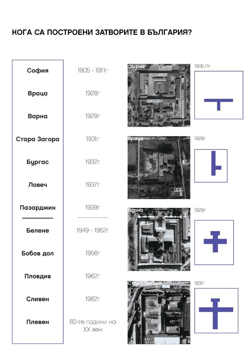
Първите български затвори са проектирани в началото на ХХ век по стандартна схема с кръстосан план с главна наблюдателна кула в центъра и жилищни корпуси с дълги коридори, от които се стига до килиите. Надзирателят наблюдава от кулата и има видимост към всички крила на сградата. Това де факто е вид паноптикум. Такива са затворите в София, Враца, Варна и Стара Загора, проектирани между 1905 и 1931 г. Характерни елементи на тези сгради са масивните огради, централните наблюдателни кули с т.нар. колело в тях и второстепенните охранителни кули. Последният нов затвор, построен в България, е Сливенският женски затвор от 1961 г.

Местата за лишаване от свобода в България се делят на няколко вида: затвори, затворнически общежития от закрит тип и затворнически общежития от открит тип. Диференцирането на лишените от свобода в съответния вид заведение се извършва според режима на изтърпяване на наказанието – специален, строг, общ и лек.
Статистически данни показват, че за последните 10 години лишените от свобода са намалели почти двойно. Това, както и откриването на нови затворнически общежития за по-леките режими, облекчава системата и дава възможност за подобряване на условията в заведенията за лишаване от свобода. Фактори като намалелия брой престъпления и респективно лишени от свобода, влизането на България в Европейския съюз и налагането на Европейските правила за затворите, както и финансирането на програми за подобряване на местата за лишаване от свобода дават оптимистичен шанс за промяна на сегашното състояние.
Какъв би могъл да бъде новият универсален архитектурен модел на тази промяна?
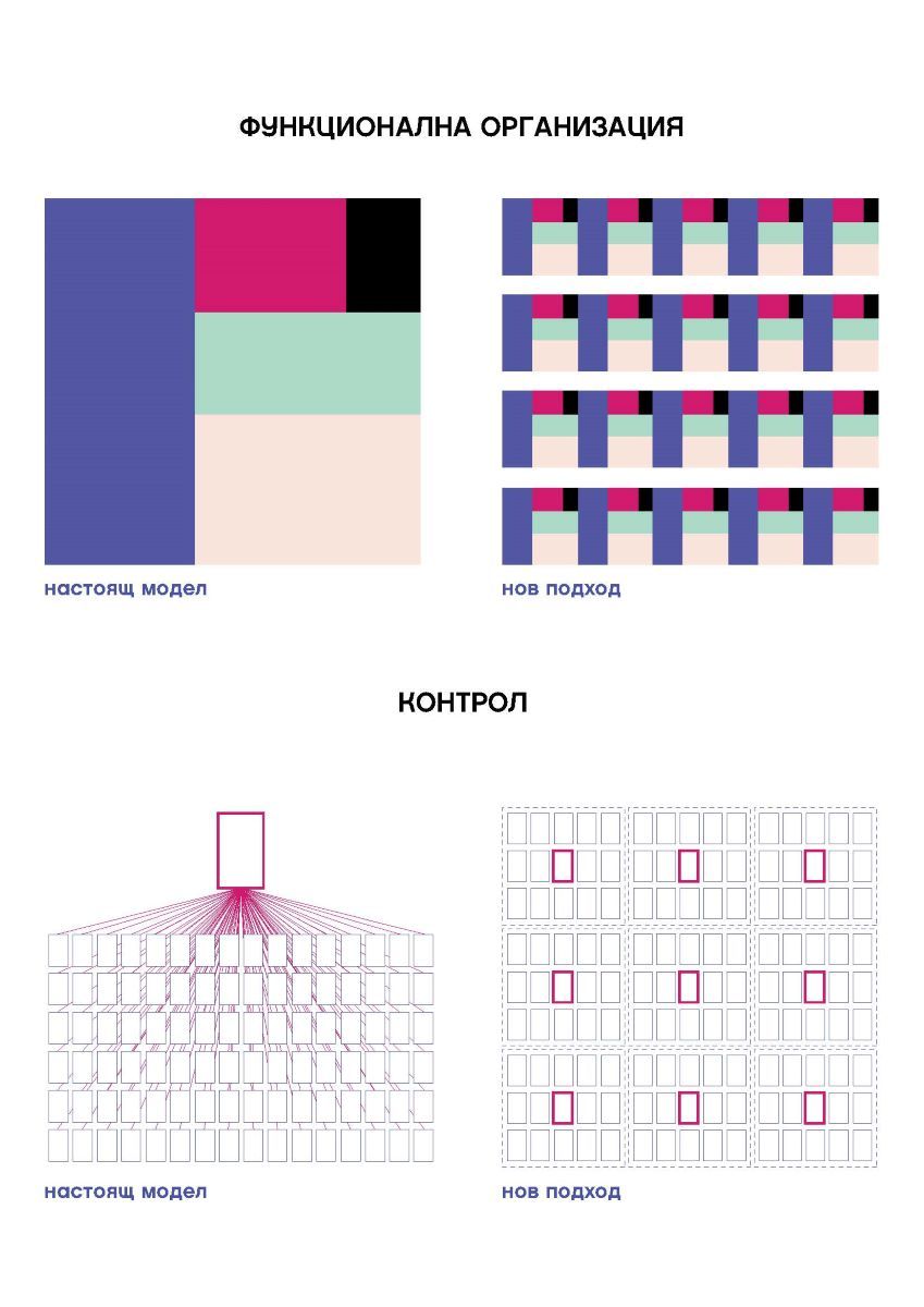
Първо, килията трябва да загуби ролята си на централно място в живота на затворниците, отстъпвайки мястото на модел, организиран на принципа на самодостатъчни жилищни единици. В рамките на всяка жилищна единица затворниците да могат сами да управляват времето си и да организират разпределението на отговорностите по отношение на общите части. Това овластява хората и предразполага към проактивно поведение. Жилищните единици да бъдат балансирана организация между индивидуални пространства за самостоятелни дейности и колективни пространства за социално взаимодействие с фокус върху вторите – отново с цел изграждане на микрообщности.
После, нужна е борба със стереотипите – премахване на плашещия образ на затворите и стигмата на лишаването от свобода. Като социална институция пенитенциарното заведение трябва, доколкото е възможно, да бъде интегрирано в общността, в която ще бъде освободен затворникът, и да взаимодейства с околността.


Разбира се, не може без бариери към външния свят за поддържане на сигурността. Но архитектурният образ трябва да деинституционализира сградата и да я интегрира в по-широката общност чрез представяне на нормализиран, съвременен, ориентиран към гражданите облик и подходящ мащаб. Затворът трябва да е във връзка с външния свят, за да не се превърне в непроницаем елемент, неотзивчив към стимулите, идващи от града.
Възможно ли е такова бъдеще на затворите? Вероятно да. Възможно ли е в България? Разбира се. Но то е в пряка връзка и с осъзнаването на властта на архитектурата да решава социални проблеми, като създава смислени пространства.
Post Syndicated from Зорница Христова original https://www.toest.bg/po-bukvite-yu-dzien/

превод Веселин Карастойчев, София, „Издателство за поезия ДА“, 2023
Признавам, че разтворих Ю Дзиен с очаквания, породени от предишния превод на Веселин Карастойчев, този на великолепния поет Бей Дао. С други думи, очаквах поезия, в която значещи са и образите, и паузите, смисловите разстояния между тях, съпоставянето; поезия, която се възприема цялостно, като калиграфски знак. „Поезия на забулената луна“ я наричат в Китай – но това, както каза някой на премиерата, е удобен начин да обезопасиш чуждия глас. Да го обявиш за неясен. Още повече че тази привидна „неяснота“ може да бъде свързана със също тъй приемливите за режима древни поетически традиции. Независимо от реалната сила на стиха.
Че Ю Дзиен пише коренно различна поезия, се вижда отведнъж. И без да четем послеслова, и без да знаем за тълпата следовници на Бей Дао и за „втвърдяването“ на тази поетика в литературна мода. Ако разтворите „Давам име на една врана“ напосоки и прочетете първото попаднало Ви стихотворение,
Може да речете, че е Гинзбърг, примерно. Заради бурната смесица от романтическа стихийност, домогване до сюблимното и постиндустриална материя, урбанистични отломки, които са част от вихрения космичен пейзаж а ла Уилям Блейк. Или заради самата форма на стихотворенията, които се доближават до изговорената реч, до „изстъплението“ в буквален смисъл – човек, който стъпва някъде и говори пред другите или пред пустошта, но говори на глас. Прави паузи, които в говоримата реч не са обозначени нито със запетаи, нито с точки, нито с други препинателни знаци – те са просто паузи, отстояния между думите. Така са маркирани и у Ю Дзиен. Или заради изобилието от неща, от думи, от образи, които следват един след друг – и тук асоциацията, разбира се, е първо Уитман, после Гинзбърг. Последният, прочее, се появява действително в едно от стихотворенията, значи не съм се догаждала напусто.
Неговият Китай е пределно и буквално съвременен; старите пътища на думите са асфалтирани, предметният свят е ремонтиран, човекът, който някога е имал „душа на царевица“, днес живее в огромен град – и не смята да се преструва, че това не е така.
Това е съвременен Китай, който по някакъв начин е по-херметичен за западното око от своята древност, защото е съвременен по свой начин; който не е директно допълнение на представата ни за себе си, а нещо друго. От една страна, този Китай е комунистически. Как се отнася поезията на Ю Дзиен към въпросния факт? Не пряко – не очаквайте някакви лозунгаджийско-бунтовни стихотворения, въпреки че поетът има какво да каже (родителите му са жертви на Културната революция, самият той прекарва младежките си години в работа по фабрики).
Ю Дзиен рисува не самата система (предполагам, и там основана на доносничеството и конформизма като цена на успеха), а ефекта ѝ върху съкровените човешки отношения. Върху приятелството и любовта. Има една серия стихотворения за срещи между приятели, които не са се виждали от много години – приятели, които разбират, че са изгубили общия си език, че няма какво да си кажат.
Две от тези стихотворения са почти диаметрално противоположни – в едното говорещият, нарекъл се в последния стих Ю Дзиен, тихо се озлобява срещу свой преуспял и зализан някогашен другар. В другото пък насреща ни сяда човек с бутилка алкохол, която до края на стихотворението пресушава и си тръгва заедно с целия си едновремешен потенциал. Любовта, прочее, присъства в момента на раздялата (като не се обичаме вече, да се разделим) и в момента на предварителното проучване… описано като полицейски разпит. Ето това описание на разпит, в който човек малодушно предава себе си до най-съкровените си неща, всъщност е най-политическото стихотворение в сборника. Въпреки че привидно иде реч за любов.
Намерила съм с какво да се хваля – все едно да се похваля, че разбирам добре стихотворението за спирането на тока. Или тези за коронавируса; има цял цикъл, като са уловени различни болезнени точки: изречението „Ясно ли е“, повтаряно при разпита на заговорилия за опасността учен; опита на човек да придаде достойнство и спокойствие на гласа си, докато съобщава по телефона, че е заразен, все едно се държи джентълменски на борда да потъващ кораб; неповторимостта на всяко име срещу статистиката на „случаите“ и т.н.

Изобщо, поезията на Ю Дзиен е обърната към реалността и се стреми да я види, стреми се да я разбере. Друг е въпросът, че постоянно се блъска в стъклената преграда пред нея; постоянно остава уловена в собственото си съзнание, колкото и да иска да постигне нещото само по себе си. Стихотворението, дало име на сборника, говори точно за това – за
Впрочем същата тема според мен е присмехулно подхваната в „Хей, свят, ела“. Ю Дзиен говори от името на човек, който в самотата си иска да приветства целия свят, всяка душа, която би дошла при него – жена, мъж, старица, мравка, комар, готов в проститутката да види невеста, в дрипавия – побратим, в покритата със струпеи баба – майка и т.н. Но когато в самотата му навлизат реални хора – съвсем банални жена, мъж, старица, мравка, комар, – те му остават напълно чужди, не будят никакво желание за общуване. Пропъжда ги, убива комара и отново започва да копнее светът да дойде при него. Въображаемият свят, разбира се.
С други думи, не бива да гледаме на поезията на Ю Дзиен като на реалистична поезия, тоест като описваща реалността. Тя е по-скоро хипнотизирана от пълнокръвието на света, от изобилието на случващото се в него и описва именно този свой захлас. Това много често е и функцията на метафората в много стихотворения – не да обясни реалността, а да добави към нея случване, размах, сюблимност. Което също си е романтически жест.
В емблематичната си колонка, започната още през 2008 г. във в-к „Култура“, Марин Бодаков ни представяше нови литературни заглавия и питаше с какво точно тези книги ни променят. Вярваме, че е важно тази рубрика да продължи. От човек до човек, с нова книга в ръка.
Post Syndicated from Crosstalk Solutions original https://www.youtube.com/watch?v=oFuUdgaAY7g
Post Syndicated from original https://xkcd.com/2790/

Post Syndicated from Amy Laresch original https://aws.amazon.com/blogs/big-data/best-practices-for-enabling-business-users-to-answer-questions-about-data-using-natural-language-in-amazon-quicksight/
In this post, we explain how you can enable business users to ask and answer questions about data using their everyday business language by using the Amazon QuickSight natural language query function, Amazon QuickSight Q.
QuickSight is a unified BI service providing modern interactive dashboards, natural language querying, paginated reports, machine learning (ML) insights, and embedded analytics at scale. Powered by ML, Q uses natural language processing (NLP) to answer your business questions quickly. Q empowers any user in an organization to start asking questions using their own language. Q uses the same QuickSight datasets you use for your dashboards and reports so your data is governed and secured. Just as data is prepared visually using dashboards and reports, it can be readied for language-based interactions using a topic. Topics are collections of one or more datasets that represent a subject area that your business users can ask questions about. To learn how to create a topic, refer to Creating Amazon QuickSight Q topics.
With automated data preparation in QuickSight Q, the model will do a lot of the topic setup for you, but there is some context that is specific to your business that you need to provide. To learn more about the initial setup work that Q does behind the scenes, check out New – Announcing Automated Data Preparation for Amazon QuickSight Q.
Business users can access Q from the QuickSight console or embedded in your website or application. To learn how to embed the Q bar, refer to Embedding the Amazon QuickSight Q search bar for registered users or anonymous (unregistered) users. To see examples of embedded dashboards with Q, refer to the QuickSight DemoCentral.
Once you have a topic shared with your business users, they can ask their own questions and save questions to their pinboard as seen in GIF 1.

QuickSight authors can also add their Q visuals straight to an analysis to speed up dashboard creation, as seen in GIF 2.

This post assumes you’re familiar with building visual analytics in dashboards or reports, and shares new and different strategies needed to build natural language interfaces that are simple to use.
In this post, we discuss the following:
If you don’t have Q enabled yet, refer to Getting started with Amazon QuickSight Q or watch the following video.
In the following examples, we often refer to two out-of-the-box sample topics, Product Sales and Student Enrollment Statistics, so you can follow along as you go. We recommend creating the topics now before continuing with this post, because they take a few minutes to be ready.
Before we jump into solutions, let’s talk about when natural language query (NLQ) capabilities are right for your use case. NLQ is a fast way for a business user who is an expert in their business area to flexibly answer a large variety of questions from a scoped data domain. NLQ doesn’t replace the need for dashboards. Instead, when designed to augment a dashboard or reporting use case, NLQ helps business users get customized answers about specific details without asking a business analyst for help.
It’s critical to have a well-understood use case because language is inherently complex. There are many ways to refer to the same concept. For example, a university might refer to “classes” several ways, such as “courses,” “programs,” or “enrollments.” Language also has inherent ambiguity—“top students” might mean by highest GPA to one person and highest number of extracurriculars to another. By understanding the use case up front, you can uncover areas of potential ambiguity and build that knowledge directly into the topic.
For example, the AWS Analytics sales leadership team uses QuickSight and Q to track key metrics for their region as part of their monthly business review. When I worked with the sales leaders, I learned their preferred terminology and business language through our usability sessions. One observation I made was that they referred to the data field Sales Amortized Revenue as “adrr”. With these learnings, I could easily add this context to the topic using synonyms, which I cover in detail below. One of the sales leaders shared, “This will be awesome for next month when I write my MBR. What previously took a couple of hours, I can now do in a few minutes. Now I can spend more time working to deliver my customer’s outcomes.” If the sales leader asked a question about “adrr” but that connection was not included in their Q topic, then the leader would feel misunderstood and revert back to their original, but slower, ways of finding the answer. Check out more QuickSight use cases and success stories on the AWS Big Data Blog.
In this section, we share a few common challenges and considerations when getting started with Q.
One pitfall to look out for is any fields with long strings, like survey write-in responses, product descriptions, and so on. This type of data introduces additional lexical complexity for readers to navigate. In other words, when an end-user asks a question, there is a higher chance that a word in one of the strings will overlap with other relevant fields, such as a survey write-in that mentions a product name in your Product field. Other non-descriptor fields can also contain overlaps. You can have two or more field names with lexical overlap, and the same across values, and even between fields and values. For example, let’s say you have a topic with a Product Order Status field with the values Open and Closed and a Customer Complaint Status field also with the values Open and Closed. To help avoid this overlap, consider alternate names that would be natural to your end-users to avoid the potential ambiguity. In our example, I’d keep the Product Order Status values and change the Customer Complaint Status to Resolved and Unresolved.
Another common pitfall that introduces unnecessary ambiguity is including calculated fields for basic aggregations that Q can do on the fly. For example, business users might track average clickthrough rates for a website or month-to-date free to paid conversions. Although these types of calculations are necessary in a dashboard, with Q, these calculated fields are not needed. Q can aggregate metrics using natural language, like simply asking “year over year sales” or “top customers by sales” or “average product discount,” as you can see in Figure 1. Defining a field with the name YoY Sales adds an additional potential answer choice to your topic, leaving end-users to select between the pre-defined YoY Sales field, or using Q’s built-in YoY aggregation capability, whereas you may already know which of these choices is likely to bring them the best outcome. If you have complex business logic built into calculated fields, those are still relevant to include (and if you create the topic from your existing analysis, then Q will bring them over.)

Figure 1: Q visual showing MoM sales for EMEA
For this post, we recommend defining a use case as a well-defined set of questions that actual business users will ask. Q gives the ability to answer questions not already answered in dashboards and reports, so simply having a dashboard or a dataset doesn’t mean you necessarily have a Q-ready use case. These questions are the real words and phrases used by business users, like “how are my customers performing?” where the word “performing” might map in the data to “sales amortized revenue,” but a business user might not ask questions using the precise data names.
Start with a single use case and the minimum number of fields to meet it. Then incrementally layer in more as needed. It’s better to introduce a topic with, for example, 10 fields and a 100% success rate of answering questions as expected vs. starting with 30 fields and a 70% success rate to help users feel confident.
To help you start small, Q enables you to create your topic in one click from your existing analysis (Figure 2).

Figure 2: Enable a Q topic from a QuickSight analysis
Q will scan the underlying metadata in your analysis and automatically select high-value columns based on how they are used in the analysis. You’ll also get all your existing calculated fields ported over to the new topic so you don’t have to re-create them.
Q knows English well. It understands a variety of phrases and different forms of the same word. What it doesn’t know is the unique terms from your business, and only you can teach it.
There are some key ways to provide Q this context, including adding synonyms, semantic types, default aggregations, primary date, named filters, and named entities. If you created your Q topic as described in the previous section, you will be a few steps ahead, but it’s always good to check the model’s work.
In a dashboard, authors use visual titles, text boxes, and filter names to help business users navigate and find their answers. With NLQ, language is the interface. NLQ empowers business users to ask their questions in their own words. The author needs to make those business lexicon connections for Q using synonyms. Your business users might refer to revenue as “gross sales,” “amortized revenue,” or any number of terms specific to your business. From the topic authoring page, you can add relevant terms (Figure 3).

Figure 3: Adding relevant synonyms
If your business users refer to the data values in multiple ways, you can use value synonyms to create those connections for Q (Figure 4). For example, in the Student Enrollment topic, let’s say your business users sometimes use First Years to map to Freshmen and so on for each classification type. If you don’t have that data directly in your dataset, you can create those mappings using value synonyms (Figure 5).

Figure 4: Configure field value synonyms

Figure 5: Example value synonyms for Student Enrollment topic
When you create a topic using automatic data prep, Q will automatically select relevant semantic types that it can detect. Q uses semantic types to understand which specific fields to use to answer vague question like who, where, when, and how many. For example, in the student enrollment statistics example, Q already set Home of Origin as Location so if someone asks “where,” Q knows to use this field (Figure 6). Another example is adding Person for the Student Name and Professor fields so Q knows what fields to use when your business users ask for “who.”

Figure 6: Semantic Type set to “Location”
Another important semantic type is the Identifier. This tells Q what to count when your business users ask questions like “How many were enrolled in biology in 2021?” (Figure 7). In this example, Student ID is set as the Identifier.

Figure 7: Q visual showing a “how many” question
Here is a list of semantic types that map to implicit question phrases:
Location: Where?Person or Organization: Who?
Identifier: How many? What is the number of?Duration: How long?Date Part: When?Age: How old?Distance: How far?Semantic types also help the model in several other ways, including mapping terms like “most expensive” or “cheapest” to Currency. There is not always a relevant semantic type, so it’s okay to leave those empty.
Q will always aggregate measure values a business user asks for, so it’s important to use measures that retain their meaning when brought together with other values. As of this writing, Q works best with underlying data that is summative, for example, a currency value or a count. Examples of metrics that are not summative are percentages, percentiles, and medians. Measures of this type can produce misleading or statistically inaccurate results when added with one another. Q can be used to produce averages, percentiles, and medians by end-users without first performing those calculations in underlying data.
Help Q understand the business logic behind your data by setting default aggregations. For example, in the Student Enrollment topic, we have student test scores for every course, which should be averaged and not summed, because it’s a percentage. Therefore, we set Average as the default and set Sum as a not allowed aggregation type (Figure 8).

Figure 8: Setting “Sum” as a “Not allowed aggregation” for a percentage data field
To ensure end-users get a correct count, consider whether the default aggregation type for each dimensional field should be Distinct Count or Count and set accordingly. For example, if we wanted to ask “how many courses do we offer,” we would want to set Courses to Distinct Count because the underlying data contains multiple records for the same course to track each student enrolled.
If we have a count, we get over 6,000 courses, which is a count of all rows that have data in the Courses field, covering every student in the dataset (Figure 9).

Figure 9: Q visual showing a count of courses
If we set the default aggregation to Distinct Count, we get the count of unique course names, which is more likely to be what the end-user expects (Figure 10).

Figure 10: Q visual showing the unique count of courses
Q will automatically select a primary date field for answering time related questions like “when” or “yoy”. If your data includes more than one date field, you may want to choose a different date than Q’s default choice. End-users can also ask about additional date fields by explicitly naming them (Figure 12). You can always specify a different date if you’d like. To review or change the primary date, go to the topic page, navigate to the Data section, and choose the Datasets tab. Expand the dataset and review the value for Default date (Figure 11).

Figure 11: Reviewing the default date
You can change the date as needed.

Figure 12: Asking about non-default dates
In a dashboard, filters are critical to allow users to focus in on their area of interest. With Q, traditional filters aren’t required because users can automatically ask to filter any field values included in the Q topic. For example, you could ask “What were sales last week for Acme Inc. for returning shoppers?” Instead of building the filters in a dashboard (date, customer name, and returning vs. new customer), Q does the filtering on the fly to instantly provide the answer.
With Q, a filter is a specific word or phrase your business users will use to instruct Q to filter returned results. For example, you have student test scores but you want a way for your users to ask about failing test scores. You can set up a filter for “Failing” defined as test scores less than 70% (Figure 13).

Figure 13: Filter configuration example using a measure
Additionally, maybe you have a field for Student Classification, which includes Freshmen, Sophomore, Junior, Senior, and Graduate, and you want to let users ask about “undergrads” vs. “graduates” (Figure 14). You can make a filter that includes the relevant values.

Figure 14: Filter configuration example using a dimension
Named entities are a way to get Q to return a set of fields as a table visual when a user asks for a specific word or phrase. If someone wanted to know “sales for retail december” and they get a KPI saying $6,169 without any extra context, it is hard to understand all data this number includes (Figure 15).

Figure 15: A Q visual showing “sales for retail december”
By presenting the KPI in a table view with other relevant dimensions, the data includes additional context making it easier to understand meaning (Figure 16).

Figure 16: A Q visual showing “sales details for retail december”
By building these table views, you can happily surprise your business users by anticipating the information they want to see without having to explicitly ask for each piece of data. The best part is your business users can easily filter the table using language to answer their own data questions. For example, in the Student Enrollment topic, we created a Student information named entity with some important student details like their name, major, email, and test scores per course.

Figure 17: Named entity example
If a university administrator wanted to reach out to students who are failing biology, they can simply ask for “student information for failing biology majors.” In one step, they get a filtered list that already includes their emails and test scores so they can reach out (Figure 18).

Figure 18: Filtering a named entity
If the university administrator wanted to also see the phone numbers of the students to send texts offering free tutoring, they could simply ask Q “Student information for failing biology majors with phone numbers.” Now, Mobile is added as the first column (Figure 19).

Figure 19: Adding a column to a named entity
Entities can also be referenced using synonyms in order to capture all the ways your business users might refer to this group of data. In our example, we could also add “student contact info” and “academic details” based on the common terminology the university admins use.
Besides looking for patterns in the data fields, ask yourself about what your business users care about. For example, let’s assume we have data for our HR specialists, and we know they care about job postings, candidates, and recruiters. Each author might think of the groups slightly differently, but as long as it’s rooted in your business jobs to be done, then your groupings are providing value. With those three groups in mind, we can sort all the data into one of those buckets. For this use case, our Candidate bucket is pretty large, with about 20 fields. We can scan the list and notice that we track information for rejected and accepted candidates, so we start splitting the metrics into two groups: Successful Candidates and Rejected Candidates. Now information like Offer Letter Date, Accept Date, and Final Salary are all in the Successful Candidate group, and related fields about Rejected Candidates are clearly grouped together.
If you’re curious about strategies for how to create entities, check out card sorting techniques.
In the Product Sales sample topic, after scanning the data, we would start with Sales, Product, and Customer as three key groupings of information to analyze. Try out the exercise on your own data and feel free to ask any questions on the QuickSight Community. To learn how to create named entities, refer to Adding named entities to a topic dataset.
After you have refined your topic, tested it out with some readers, and made it available for a larger audience, it’s important to follow two strategies to drive adoption.
First, provide your business users with support. Support might look like a short tutorial video or newsletter announcement. Consider keeping an open channel like a Slack or Teams chat where active users can post questions or enhancements.
Here at Amazon, the Prime team has a dedicated Product Manager (PM) for their embedded Q application that they call PrimeQ. The PM hosts regular demo and training sessions where the Prime team can ask them any questions and get ideas about what types of answers they can get. The PM also sends out a monthly newsletter to announce the availability of new data and topics along with sample questions, FAQs, and quotes from Prime team members who get value out of Q. The PM also has an active Slack channel where every single question gets answered within 24 hours, either by the PM or a data engineer on the Prime team.
Pro tip: Make sure your business users know who they can reach out to if they get stuck. Avoid the black box of “reach out to your author” so readers feel confident their questions will be answered by a known person. For embedded applications, be sure to build an easy way to get support.
Second, maintain a healthy feedback loop. Look at the usage data directly in the product and schedule 1-on-1 sessions with your readers. Use the usage data to track adoption and identify readers who are asking unanswerable questions (Figure 20). Engage with both your successful and struggling readers to learn how to continue to iterate and improve the experience. Talking to business users is especially important to uncover the implicit ambiguity of language.
Another example here at Amazon, after first launching the Revenue Insights topic for the AWS Analytics sales team, a QuickSight Solution Architect (SA) and myself checked the usage tab on a daily basis to track unanswerable questions and directly reach out to the sales team member to let them know how to adjust their question or that we made a change so their question would now work. For example, we initially had a field turned off for Market Segment and noticed a question from a sales leader asking about sales by segment. We turned the field on and let him know those questions would now work. The SA and I have a Slack channel with other stakeholders so we can troubleshoot asynchronously with ease. Now that the topic has been available for several months, we check the usage tab on a weekly basis.

Figure 20: User Activity tab in Q
In this post, we discussed how language is inherently complex and what context you need to provide Q to teach the system about your unique business language. Q’s automated data prep will get you started, but you need to add the context that is specific to your business user’s language. As we mentioned at the start of the post, consider the following:
Follow this post to enable your business users to answer questions of data using natural language in QuickSight.
Ready to get started with Q? Watch our quick tutorial on enabling QuickSight Q.
Want some tutorial videos to share with your team? Check out the following:
To see how Q can answer the “Why” behind data changes and forecast future business performance, refer to New analytical questions available in Amazon QuickSight Q: “Why” and “Forecast”.
 Amy Laresch is a product manager for Amazon QuickSight Q. She is passionate about analytics and is focused on delivering the best experience for every QuickSight Q reader. Check out her videos on the @AmazonQuickSight YouTube channel for best practices and to see what’s new for QuickSight Q.
Post Syndicated from original https://lwn.net/Articles/934679/
The C language does not provide the sort of resource-management features
found in more recent languages. As a result, bugs involving
leaked memory or failure to release a lock are relatively common in
programs written in C — including the kernel. The kernel project has never
limited itself to the language features found in the C standard, though;
kernel developers will happily
use extensions provided by compilers if they prove helpful. It looks like
a relatively simple compiler-provided feature may lead to a significant
change in some common kernel coding patterns.
Post Syndicated from Srividya Parthasarathy original https://aws.amazon.com/blogs/big-data/efficiently-crawl-your-data-lake-and-improve-data-access-with-aws-glue-crawler-using-partition-indexes/
In today’s world, customers manage vast amounts of data in their Amazon Simple Storage Service (Amazon S3) data lakes, which requires convoluted data pipelines to continuously understand the changes in the data layout and make them available to consuming systems. AWS Glue crawlers provide a straightforward way to catalog data in the AWS Glue Data Catalog that removes the heavy lifting when it comes to schema management and data classification. AWS Glue crawlers extract the data schema and partitions from Amazon S3 to automatically populate the Data Catalog, keeping the metadata current.
But with data growing exponentially over time, the number of partitions in a given table can grow significantly. Because analytics services like Amazon Athena query a table containing millions of partitions, the time needed to retrieve the partition increases and can cause query runtime to increase.
Today, AWS Glue crawler support has been expanded to automatically add partition indexes for newly discovered tables to optimize query processing on the partitioned dataset. Now, when the crawler creates a new Data Catalog table during a crawler run, it also creates a partition index by default, with the largest permutation of all numeric and string type partition columns as keys. The Data Catalog then creates a searchable index based on these keys, reducing the time required to retrieve and filter partition metadata on tables with millions of partitions. The creation of partition indexes benefits the analytics workloads running on Athena, Amazon EMR, Amazon Redshift Spectrum, and AWS Glue.
In this post, we describe how to create partition indexes with an AWS Glue crawler and compare the query performance improvement when accessing the crawled data with and without a partition index from Athena.
We use an AWS CloudFormation template to create our solution resources. In the following steps, we demonstrate how to configure the AWS Glue crawler to create a partition index using either the AWS Glue console or the AWS Command Line Interface (AWS CLI). Then we compare the query performance improvements using Athena.
To follow along with this post, you must have access to an AWS Identity and Access Management (IAM) administrator role to create resources using AWS CloudFormation.
The CloudFormation template generates the following resources:
Complete the following steps to set up the solution resources:
blog_partition_index_crawlerdb.
DatabaseName and GlueCrawlerName.
Some of the resources that this stack deploys incur costs when in use.
To configure and run the AWS Glue crawler, complete the following steps:
crawler blog-partition-index-crawler and choose Edit.

Alternatively, you can configure your crawler using the AWS CLI (provide your IAM role and Region):
This is highly partitioned dataset and will take approximately 90 minutes to complete.

In the AWS Glue database blog_partition_index_crawlerdb, verify that the table highly_partitioned_table is created.
By default, the crawler determines an index based on the largest permutation of partition columns of valid column types in the same order of partition columns, which are either numeric or string. For the table created by the crawler (highly_partitioned_table), we have partition columns year (string), month (string), day (string), and hour (string).

Based on this definition, the crawler created an index on the permutation of year, month, day, and hour. The crawler created the indexes prefixed with crawler_ on any partition index created by default.
Verify the same by navigating to the table highly_partitioned_table on the AWS Glue console and choosing the Indexes tab.

The crawler was able to crawl the S3 data source and successfully populate the partition indexes for the table.
First, we query the table in Athena without using the partition index. To verify the tables using Athena, complete the following steps:
crawler-primary-workgroup as the Athena workgroup and choose Acknowledge.
The following screenshot shows the query took approximately 32 seconds without filtering enabled using the partition index.

The following screenshot shows the query took only 700 milliseconds, which is much faster with filtering enabled using the partition index.

To avoid unwanted charges to your AWS account, you can delete the AWS resources:
In this post, we explained how to configure an AWS crawler to create partition indexes and compared the query performance when accessing the data with indexes from Athena.
If no partition indexes are present on the table, AWS Glue loads all the partitions of the table, and then filters the loaded partitions, which results in inefficient retrieval of metadata. Analytics services like Redshift Spectrum, Amazon EMR, and AWS Glue ETL Spark DataFrames can now utilize indexes for fetching partitions, resulting in significant query performance.
For more information on partition indexes and query performance across various analytical engines, refer to Improve Amazon Athena query performance using AWS Glue Data Catalog partition indexes and Improve query performance using AWS Glue partition indexes.
Special thanks to everyone who contributed to this crawler feature launch: Yuhang Chen, Kyle Duong,and Mita Gavade.
 Srividya Parthasarathy is a Senior Big Data Architect on the AWS Lake Formation team. She enjoys building data mesh solutions and sharing them with the community.
 Sandeep Adwankar is a Senior Technical Product Manager at AWS. Based in the California Bay Area, he works with customers around the globe to translate business and technical requirements into products that enable customers to improve how they manage, secure, and access data.
Post Syndicated from original https://lwn.net/Articles/934561/
Darrick Wong has been doing work on XFS online
repair for a number of years
and things are getting to the point where most of the filesystem-internal work
has been completed and is under review. The work remaining mostly concerns
the user-space side
to set up a periodic scan and repair cycle, so he wanted to discuss what
user space needs from this kind of feature in a filesystem session at the
2023 Linux Storage, Filesystem,
Memory-Management and BPF Summit that he led remotely. The session may
not have gone quite as he hoped, as it got somewhat derailed by topics that
spilled over from the earlier session on
unprivileged image mounts.
Post Syndicated from Rohit Kumar original https://www.servethehome.com/insane-48-port-2-5gbe-2x-25gbe-2x-10gbe-managed-chinese-e-sports-cafe-and-hotel-switch-microchip-micron-sandisk/
We show an insane and popular 48-port 2.5GbE switch with 25GbE. Designed at under $400 this switch is powering hotels and e-Sports cafes
The post Insane 48-Port 2.5GbE 2x 25GbE 2x 10GbE Managed Chinese e-Sports Cafe and Hotel Switch appeared first on ServeTheHome.
Post Syndicated from Venkata Kampana original https://aws.amazon.com/blogs/big-data/part-1-enable-data-collaboration-among-public-health-agencies-with-aws-clean-rooms/
In this post, we show how you can use AWS Clean Rooms to enable data collaboration between public health agencies. Public health governmental agencies need to understand trends related to a variety of health conditions and care across populations in order to create policies and treatments with the goal of improving the well-being of the various communities they serve.
In order to do this, these agencies need to analyze data from many sources, such as clinical organizations, non-clinical community organizations, and administrative data from other government agencies, so they can identify trends around health conditions and treatments across populations. Public health needs to understand what is happening to populations within the communities they serve.
Because they are looking at populations at risk, they need the flexibility of a line list of cases, stripped of personally identifiable information (PII). With this information, they can assess risk based on a variety of demographic and social factors available in the data sources without divulging PII. The list gives them flexibility to apply more complex analyses, such as regression, on the linked data as well. Programs like MENDS, MDPHnet, and CODI have explored using clinical data in distributed networks to understand the burden of chronic diseases in communities for years. Challenges facing these programs include complex data sharing rules and distributed analytics approaches, across networks of data providers. MENDS and MDPHnet, for example, run analytics at the organization level without deduplicating across sites. Individual queries are pushed to each site where they are processed and reviewed by humans, and combined output is sent to the public health agency.
AWS Clean Rooms offers an opportunity to reduce the burden on data providers in programs like these, while enabling public health agencies to analyze data using their own queries and mitigate risks to data privacy by preventing access to the underlying raw data.
AWS Clean Rooms was first announced at AWS re:Invent 2022, and is now generally available. AWS Clean Rooms allows customers and their partners to more easily and securely collaborate on their collective datasets—without sharing or copying the underlying data with each other. AWS Clean Rooms provides a broad set of privacy-enhancing controls that help protect sensitive data, including query controls, query output restrictions, query logging, and cryptographic computing tools.
With AWS Clean Rooms, you can collaborate and analyze data with other parties in the collaboration without either party having to share or copy the raw data. AWS Clean Rooms is a stateless service; it doesn’t store the data. Instead, it reads the data from where it lives, applies restrictions that protect each participant’s underlying data at query runtime, and returns the results. Queries can be written to intersect and analyze data sources using common metadata elements (for example, geography, shared identifiers, or other demographic factors), generating row-level lists of the overlap between the data sources or aggregated counts by population, condition, or other strata.
AWS Clean Rooms helps public health agencies analyze collective data to gain a more complete view of the health and well-being of their communities, while maintaining the security and privacy of the data.
Before we get started with AWS Clean Rooms, let’s first talk about some of the service’s key concepts:
Getting started with AWS Clean Rooms is a four-step process:
For this walkthrough, you need the following:
You must define your collaboration configuration on the AWS Clean Rooms console, via the AWS Command Line Interface (AWS CLI), or with an AWS SDK. We demonstrate how to configure this on the console.


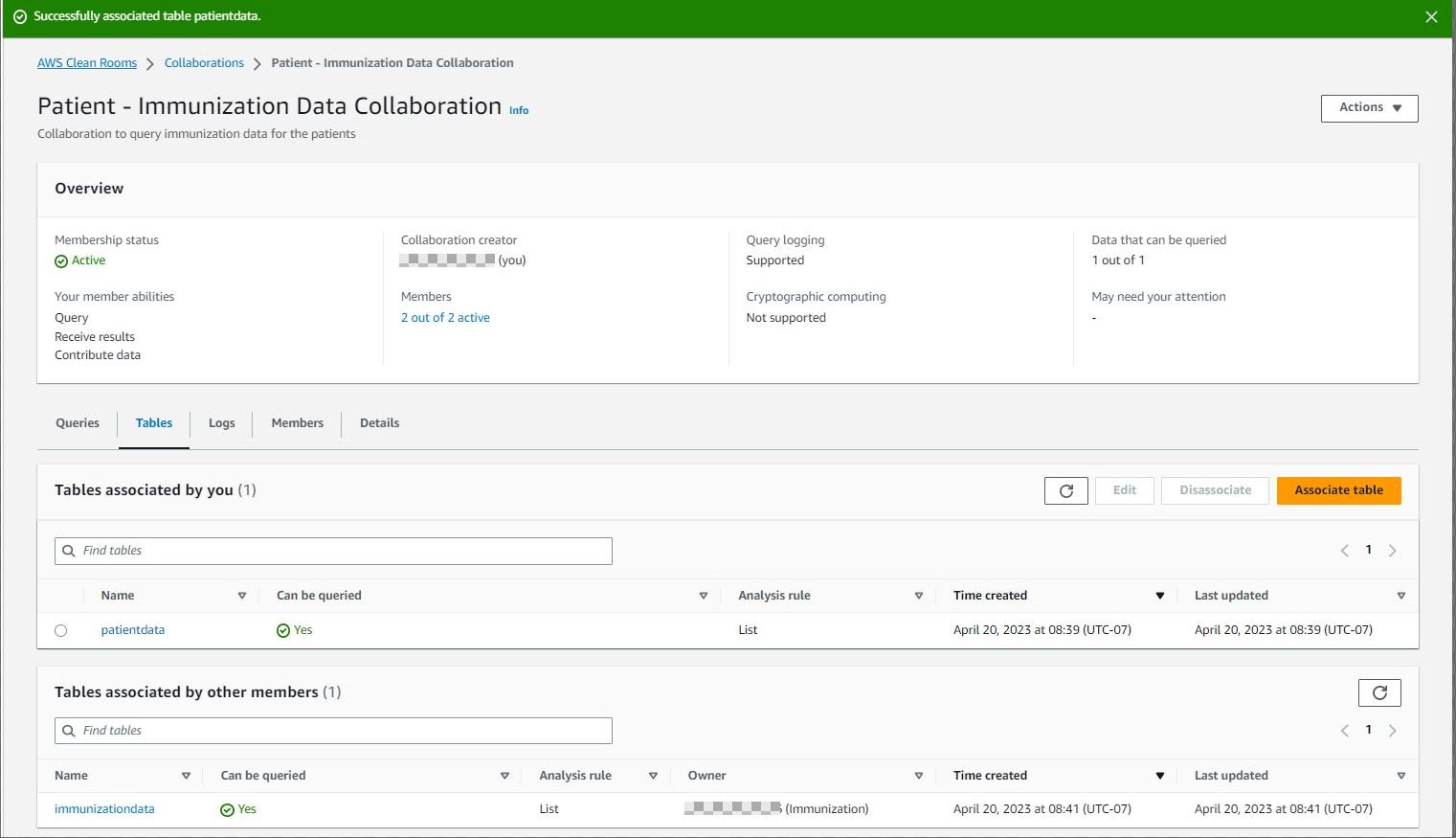
Congratulations on creating your first collaboration! You can see the collaboration details on the Collaborations page.

Each collaboration member can log in to AWS Clean Rooms console, review the invitation, and decide to join the collaboration by following these steps:

On the details page, you can review the member abilities.


After you create your membership, your member status is changed to Active on the collaboration dashboard.

AWS Clean Rooms doesn’t require you to make a copy of the data because it reads the data from Amazon S3. This eliminates the need to copy and load your data into destinations outside your respective AWS account, or use third-party services to facilitate data sharing.
Each collaboration member can create configured tables, an AWS Clean Rooms resource that contains reference to the AWS Glue Data Catalog with underlying data that defines how that data can be used. The configured table can be used across many collaborations.

For each selected table, you can determine which columns can be accessed in the collaboration.
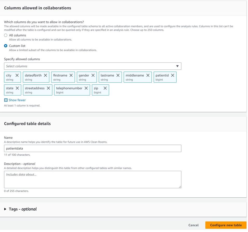
In addition to column-level access controls, AWS Clean Rooms provides fine-grained query controls called analysis rules. With built-in and flexible analysis rules, you can tailor queries to specific business needs. As discussed earlier, AWS Clean Rooms provides two types of analysis rules:
Both rule types allow data owners to mandate a join between their datasets and the datasets of the collaborator running the query. This limits the results to just their intersection of the collaborators datasets.


You will see the message Successfully configured list analysis rule on the configured tables page.


The collaboration page will display a list of tables that are associated by you to the collaboration.
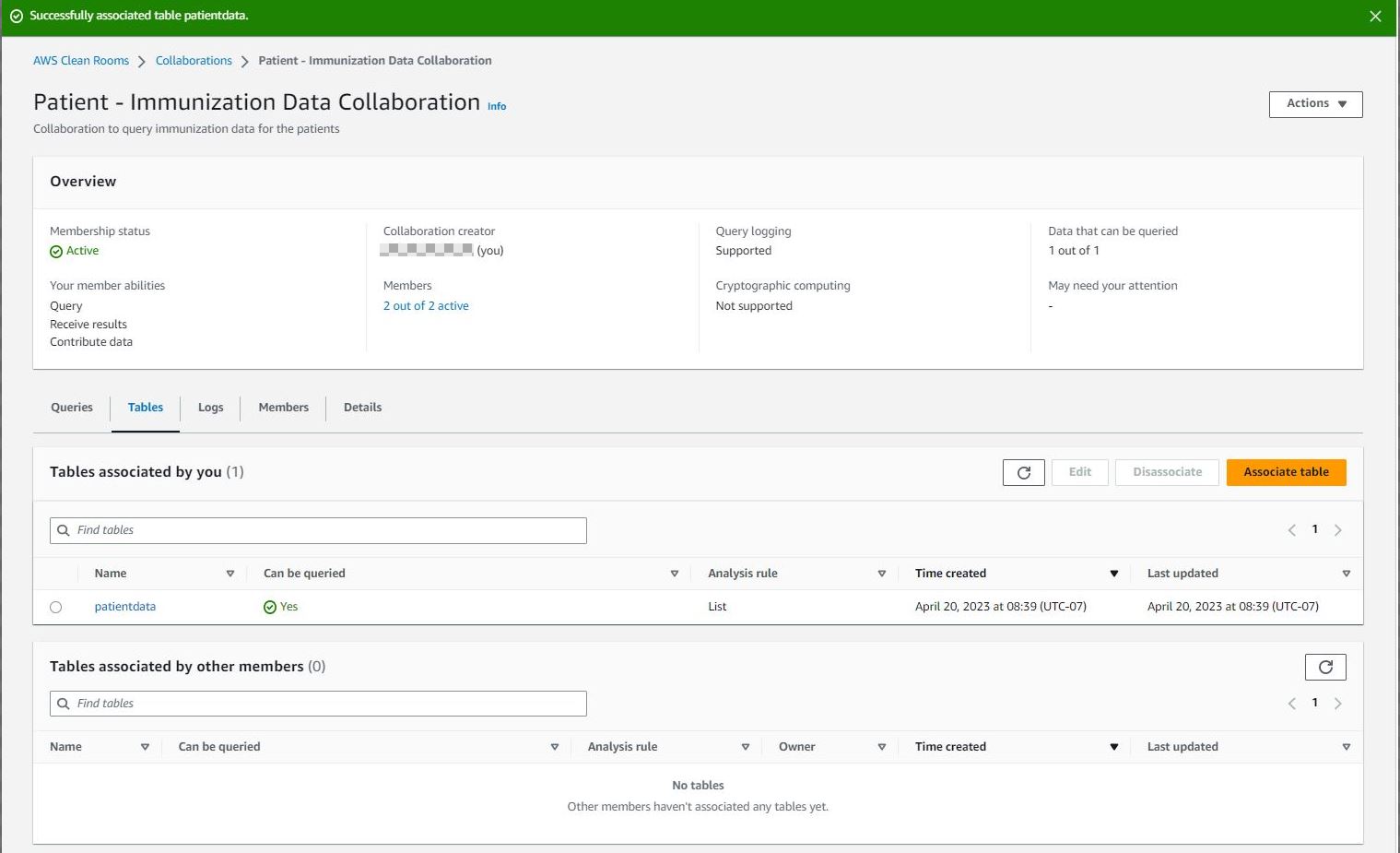
Each member of the collaboration must repeat the aforementioned steps to associate their AWS Glue Data Catalog tables to the collaboration. For this post, the other members of the collaboration follow these same steps to associate their data to the collaboration. Then the collaboration will list all tables associated by other members.
After defining the analysis rules on the configured tables and associating them to the collaboration, the members who can query and receive results can start writing queries according to the restrictions defined by each participating collaboration member. The following section includes example collaboration queries.
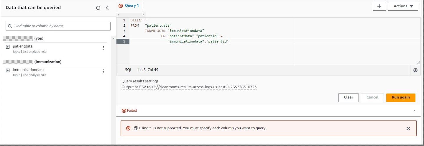
The following screenshot is an example of a query that won’t be successful because * is not supported. Column names must be specified in the query.
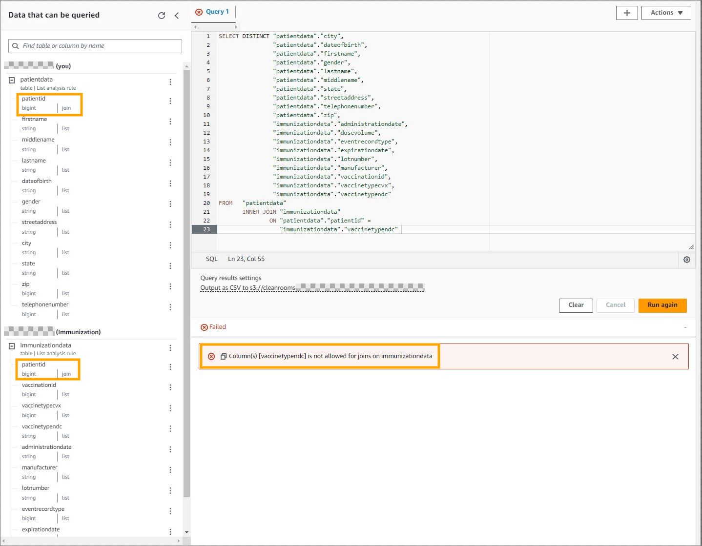
The following screenshot is an example of a query that won’t be successful because you can’t link columns that members restricted in your joins.
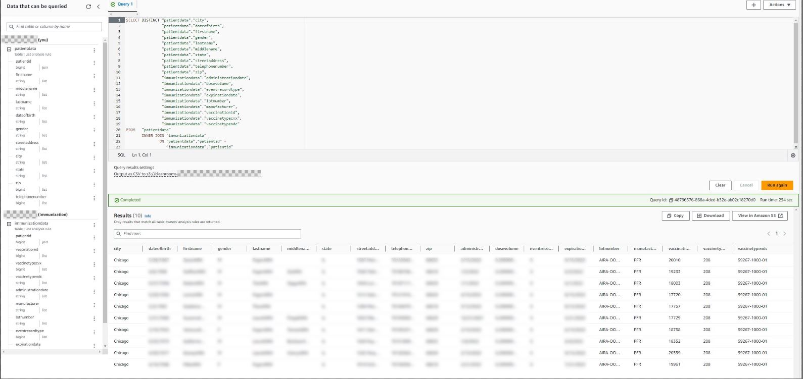
The following screenshot is an example of a query that will be successful because it uses permitted columns (columns that are part of the list analysis rule) in the select clause and join condition.
The sample datasets (Patient and Immunization) used in this post include a unique identifier (patient ID). However, in a real-world scenario, this might not be the case. In those situations, you may consider using privacy-preserving record linkage (PPRL) to create a unique deidentified token. For example, the CDC’s CODI program deduplicates across data owners by obfuscating PII behind each organization’s firewall in a standardized way. That obfuscated information is joined to create a unique deidentified token for each individual that is analyzed across data sources. If public health agencies want to conduct analyses based on individually linked longitudinal data, they could apply PPRL to each data source and use that metadata element to link the data sources in AWS Clean Rooms before conducting their analytics.
As part of this walkthrough, you provisioned an AWS Clean Rooms collaboration, invited other members to join the collaboration, and configured tables. To delete these resources, refer to Leaving the collaboration and Disassociating configured tables.
In this post, we showed you how to create a collaboration, invite other members to the collaboration, configure existing AWS Glue Catalog tables, apply analysis rules, and run sample queries on the AWS Clean Rooms console. In Part 2 of this series, we demonstrate how to automate query runs using AWS Lambda, query the results using Amazon Athena, and publish dashboards using Amazon QuickSight.
 Venkata Kampana is a Senior Solutions Architect in the AWS Health and Human Services team and is based in Sacramento, CA. In that role, he helps public sector customers achieve their mission objectives with well-architected solutions on AWS.
 Dr. Dawn Heisey-Grove is the public health analytics leader for Amazon Web Services’ state and local government team. In this role, she’s responsible for helping state and local public health agencies think creatively about how to achieve their analytics challenges and long-term goals. She’s spent her career finding new ways to use existing or new data to support public health surveillance and research.
 Jim Daniel is the Public Health lead at Amazon Web Services. Previously, he held positions with the United States Department of Health and Human Services for nearly a decade, including Director of Public Health Innovation and Public Health Coordinator. Before his government service, Jim served as the Chief Information Officer for the Massachusetts Department of Public Health.
Post Syndicated from original https://www.backblaze.com/blog/making-sense-of-ssd-smart-stats/

Over the past several years, folks have come to embrace the solid state drive (SSD) as their standard data storage device. It’s gotten to the point where people are breathlessly predicting the imminent death of the venerable hard drive. While we don’t see the demise of the hard drive happening any time soon, SSDs are here to stay and we want to share what we know about them. To that end, we’ve previously compared hard drives and SSDs as it relates to power, reliability, speed, price, and so on. But, the one area we’ve left primarily unexplored for SSDs is SMART.
SMART—or, more properly, S.M.A.R.T.—stands for Self Monitoring, Analysis, and Reporting Technology. This is a monitoring system built into hard drives and SSDs whose primary function is to detect and report on the state of the drive by populating specific SMART attributes. These include time-in-service and temperature, as well as reliability-based attributes for media condition, operational efficiency, and many more.
Both hard drives and SSDs populate SMART attributes, but given how different these drive types are, the information produced is quite different as well. For example, hard drives have sectors, while SSDs have pages and blocks. Let’s take a look at the common attributes of hard drives and SSDs, and then we’ll dig into the SSD SMART attributes we’ve found useful, interesting, or just weird.
For each SSD model, the drive manufacturer decides which SMART attributes to populate. Attributes are numbered from 1 to 255, with raw and normalized values for each attribute. Some SMART reference material will also list attributes in hexadecimal (HEX), for example, decimal 12 will also be shown as “HEX 0C.”
At Backblaze, we have over a dozen different SSD models in service, and we pull daily SMART stats from each. To simplify the task at hand for the purposes of this blog post, we chose three SSD models, one each from Seagate, Western Digital, and Crucial, to show the similarities and differences between the models. All three are 250GB SSDs.
To that end, we have created a table of the SMART attributes used by each of those three drive models. You can download a PDF of the table, or jump to the end of this post to view the table. Things to note about the table:
One of the things you’ll notice as you examine the list of attributes is that there are several which have similar names, but are different attribute numbers. That is, different vendors use a different attribute for basically the same thing. This highlights a deficiency in SMART: Participation is voluntary. While the vendors try to play nice with each other, who uses a given attribute for what purpose is subject to the whims, patience, and persistence of the many SSD manufacturers in the market today.
Often manufacturers have created their own SMART monitoring tools to use on their drives. As they add, change, and delete the SMART attributes they use, they update their tools. Drive agnostic tools such as smartctl, which we use, have to chase down updates that have occurred in each of the manufacturer’s homegrown SMART monitoring tools. There are other tools out there as well. DriveDX is another vendor-agnostic SSD monitoring tool, and here’s a link to their release notes page. They made 38 updates in release 1.10.0 (700) alone just to keep up with the drive manufacturers.
Making things more complicated, manufacturers differ widely in how they advertise the attributes and definitions they use. Kingston, for example, is very good about publishing a table of named SMART attributes and definitions for each of their drives, whereas similar information for Western Digital SSDs is difficult to find in the public domain. The net result is that agnostic SMART tools such as smartctl, DriveDx, and others have to work extra hard to keep up with new, updated, and deleted attributes.
Of the 44 attributes we list in our table, only five are common for all three of the SSD models we are examining. Let’s start with the three of the common attributes that are also common to nearly every hard drive in production today.
These two attributes are specific to SSDs and are common to all three of the models we are examining.
As noted, only five of the 44 SMART attributes are common between our three SSD models. This lack of commonality, 11%, seemed low to us, and we wondered what the commonality was between the SMART attributes on the hard drive models we use. We reviewed the SMART attributes for three 14TB hard drive models in our drive stats data set, one model each from Seagate, Western Digital, and Toshiba. We found that 42% of the SMART attributes were common between the three models. That’s nearly four times more than the SSD commonality, but admittedly less than we thought.
For the purpose at hand, we’ll define a useful attribute as something that clearly indicates the health of the SSD. That led us to focus on two concepts: Lifetime remaining (or used) percentage, and logical block addressing (LBA) read/write counts. Let’s take a look at how each of the drive models reports on these attributes.
SMART 169: Remaining Lifetime Percentage (Western Digital)
This attribute measures the approximate life left from a combination of program-erase cycles and available reserve blocks of the device. A brand new SSD will report a value of “100” for the Normalized value and decrease down to “0” as the drive is used.
SMART 202: Percentage of Lifetime Used (Crucial)
This attribute measures how much of the drive’s projected lifetime has been used at any point in time. For a brand new drive, the attribute will report “0”, and when its specified lifetime has been reached, it will show “100,” reporting that 100 percent of the lifetime has been used.
SMART 231: Life Left (Seagate)
This attribute indicates the approximate SSD life left, in terms of program/erase cycles or available reserved blocks. A brand new SSD has a normalized value of “100” and decreases from there with a threshold value at “10” indicating a need for replacement. A value of “0” may mean that the drive is operating in read-only mode.
All three use program/erase cycles (SMART 232) and available reserved blocks (SMART 170) to compute their percentages, although as is seen, SMART 202 counts up, while the other two count down. Lifetime, as defined here, is relative. That is you could be at 50% lifetime after six months or six years depending on the SSD usage.
In an SSD, data is written to and read from a page, also known as a NAND page. A group of pages forms a block. The LBA written/read count is just that, a count of blocks written/read. Each time a block is written or read the respective SMART attribute counter increases by one. For example, if various pieces of data on the pages within a single block are read 10 times, it will increase the SMART counter by 10.
SMART 241: LBAs Written (Seagate and Western Digital)
Total count of LBAs written.
SMART 242: LBAs Read (Seagate and Western Digital)
Total count of LBAs read.
SMART 246: Cumulative Host Sectors Written (Crucial)
LBAs written due to a computer request. Note that the name of this attribute seems incorrect as it states sectors versus blocks.
Crucial also counts NAND pages written due to a computer request (SMART 247) and NAND pages written due to a background operation such as garbage collection (SMART 248). Crucial does not seem to have a SMART attribute for total count of LBAs read. Nor does it seem to record LBAs written for background operations.
Below we’ve gathered several SSD SMART attributes we found interesting and one could argue potentially useful. In no particular order, let’s take a look.
SMART 230: Drive Life Protection Status (Western Digital)
This attribute indicates whether the SSD’s usage trajectory is outpacing the expected life curve. This attribute implies a couple of interesting things. First, there is a usage trajectory calculation and value. This could be SMART 169 noted previously. Second, there is a defined expected life. We assume that the expected life curve is fixed for a given SSD model and perhaps uses the warranty period as its zero date, but we’re only guessing here.
SMART 210: RAIN Successful Recovery Page Count (Crucial)
Redundant Array of Independent NAND (RAIN) is similar to gaining data redundancy using RAID in a drive array, except RAIN redundancy is accomplished within the drive, i.e., all the data written to this SSD is made redundant on the SSD itself. This redundancy is not free and either consumes some of disk space from the total space specified (250GB in this case), or uses additional space not counted in the total. Either way, this is a really cool feature and allows for data to be recovered transparently to the user even when initially it couldn’t be read due to a bad page or block.
SMART 232: Endurance Remaining (Seagate and Western Digital)
The number of physical erase cycles completed on the SSD as a percentage of the maximum physical erase cycles the drive is designed to endure. At first look, this seems similar to SMART 231 (Life Left), but this attribute does not consider available reserved blocks as part of its calculus. Still, this attribute could be a harbinger of what’s to come, as erasing SSD blocks at an accelerated rate often leads to having to utilize available reserved blocks downstream as the SSD cells wear out.
SMART 233: Media Wearout Indicator (Seagate and Western Digital)
Similar to SMART 232 (but without the math) as this attribute records the count of the actual NAND erase cycles. The normalized value starts at 100 for a new drive and decreases to a minimum of 1. As it decreases, the NAND erase cycles count (raw value) increases from 0 to the maximum-rated number of cycles.
SMART 171: SSD Program Fail Count (Western Digital and Crucial) and SMART 172: SSD Erase Count Fail (Western Digital and Crucial)
Both of these attributes count their respective failures (Program Fail and Erase Count) from when the drive was deployed. As a drive ages, one would expect these counts to increase and eventually pass some threshold value which would indicate a problem. While this is helpful in determining the health of a drive, these attributes alone provide only a partial picture as they can miss a rapid acceleration of failures over a short period of time.
There are a handful of attributes which seem odd based on our table and the attribute names and the definitions we have found. We’d like to point these out to start the conversation—If anyone can shed some light on these oddities, jump in the comments. Your input is much appreciated.
SMART 16: Total LBAs Read (Seagate)
There are two odd things here. First, the definition states that this attribute is only found on select Western Digital hard drive models—yet it was found in most of our Seagate SSDs. This could be a definition problem, but then there’s the second thing: Seagate SSDs record Total LBAs Read in attribute 242 (noted above). So, it seems it could also be an attribute name problem.
SMART 17: Unknown (Seagate)
We could not find any information on SMART 17, except for the fact that our Seagate drives report on this attribute.
SMART 196: Reallocation Event Count (Crucial), SMART 197: Current Pending Sector Count (Crucial), and SMART 198: Uncorrectable Sector Count (Crucial)
Our Crucial drives report values for these attributes, but this is another case where the names and definitions don’t make sense, as they are talking about sectors which are hard drive-specific.
SMART 206: Flying Height (Crucial)
Another attribute reported by our Crucial drives which makes no sense based on the name and definition. I think we can all agree that measuring the flying height of the cells within an SSD is not meaningful.
The questions around the Crucial reported attributes could be straightforward to answer as Crucial has their own free SMART monitoring software, Storage Executive. If you are using this software, we’d appreciate any info you can share on the Crucial names and definitions of these attributes.
Many of us have an external hard drive or two sitting on a shelf somewhere acting as a backup or perhaps even an archive of our data. Every so often, we take out one of those drives, plug it in, and hope it spins up. This can go on for years.
Can SSDs be used for offline data storage, and if so how long can they safely remain unplugged? It’s a good question and one that has been debated many times over the years with time frames ranging from a few weeks to several years. The current thinking is that when an SSD is new, it can safely store your data without power for a year or so, but as the drive wears out the data retention period begins to diminish.
This begs the question: How worn out is your SSD? For Crucial SSDs, the answer is SMART 202: Percentage Lifetime Used. We discussed this attribute earlier in relation to drive life, but it also plays a role in data retention when the drive is unpowered. Using the normalized value, Crucial estimates the following:
In theory, you should be able to use the SMART 231: Life Left (Seagate) or SMART 169: Remaining Lifetime Percentage (Western Digital) to perform the same analysis as was done above with SMART 202 and the Crucial SSD model. Remember that these two attributes (231 and 169) count downward, that is “100” is good and “0” is bad. All that said, this is just a theory, as we’ve found no documentation this is actually the case (but it does seem to make sense).
It’s great that SSD manufacturers are using SMART attributes to record relevant information about the status and health of their drive models. It’s also great that many manufacturers also provide software that monitors these SMART stats and provides the user feedback. All is wonderful when you are buying all your SSDs from the same manufacturer. But that’s just not the reality for most IT shops who are managing servers, networking gear, and so on from different vendors. It is also not the reality when it comes to running a cloud storage company.
Having accurate, up-to-date, vendor agnostic SSD monitoring tools is important to many organizations as part of their ability to cost effectively manage their systems and keep them healthy. Having to use a multitude of different tools to monitor SSDs doesn’t benefit anyone. Maybe it’s time we take SMART for SSDs beyond voluntary and look to standardize the attributes and their names and definitions across the board for all SSD manufacturers.
Multiple sources were consulted in researching this post, they are listed below. We may have missed one or two sources, and we apologize in advance if we did.
We only used sources which are available to us without purchasing something. That is, we didn’t buy agnostic monitoring applications or purchase a specific manufacturer’s SSD to have something to use their free monitoring application on. We took our Drive Stats data and then, just like you, we ventured into the internet to search out SSD SMART attribute information that was publicly available.
The following table contains the SMART attributes for the three SSD models listed. These attributes are collected by the smartctl utility within the smartmon toolset.
The post Making Sense of SSD SMART Stats appeared first on Backblaze Blog | Cloud Storage & Cloud Backup.
Post Syndicated from Kiran Anand original https://aws.amazon.com/blogs/big-data/enable-remote-reads-from-azure-adls-with-sas-tokens-using-spark-in-amazon-emr/
Organizations use data from many sources to understand, analyze, and grow their business. These data sources are often spread across various public cloud providers. Enterprises may also expand their footprint by mergers and acquisitions, and during such events they often end up with data spread across different public cloud providers. These scenarios can create the need for AWS services to remotely access, in an ad hoc and temporary fashion, data stored in another public cloud provider such as Microsoft Azure to enable business as usual or facilitate a transition.
In such scenarios, data scientists and analysts are presented with a unique challenge when working to complete a quick data analysis because data typically has to be duplicated or migrated to a centralized location. Doing so introduces time delays, increased cost, and higher complexity as pipelines or replication processes are stood up by data engineering teams. In the end, the data may not even be needed, resulting in further loss of resources and time. Having quick, secure, and constrained access to the maximum amount of data is critical for enterprises to improve decision-making. Amazon EMR, with its open-source Hadoop modules and support for Apache Spark and Jupyter and JupyterLab notebooks, is a good choice to solve this multi-cloud data access problem.
Amazon EMR is a top-tier cloud big data solution for petabyte-scale data processing, interactive analytics, and machine learning using open-source frameworks such as Apache Spark, Apache Hive, and Presto. Amazon EMR Notebooks, a managed environment based on Jupyter and JupyterLab notebooks, enables you to interactively analyze and visualize data, collaborate with peers, and build applications using EMR clusters running Apache Spark.
In this post, we demonstrate how to set up quick, constrained, and time-bound authentication and authorization to remote data sources in Azure Data Lake Storage (ADLS) using a shared access signature (SAS) when running Apache Spark jobs via EMR Notebooks attached to an EMR cluster. This access enables data scientists and data analysts to access data directly when operating in multi-cloud environments and join datasets in Amazon Simple Storage Service (Amazon S3) with datasets in ADLS using AWS services.
Amazon EMR inherently includes Apache Hadoop at its core and integrates other related open-source modules. The hadoop-aws and hadoop-azure modules provide support for AWS and Azure integration, respectively. For ADLS Gen2, the integration is done through the abfs connector, which supports reading and writing data in ADLS. Azure provides various options to authorize and authenticate requests to storage, including SAS. With SAS, you can grant restricted access to ADLS resources over a specified time interval (maximum of 7 days). For more information about SAS, refer to Delegate access by using a shared access signature.
Out of the box, Amazon EMR doesn’t have the required libraries and configurations to connect to ADLS directly. There are different methods to connect Amazon EMR to ADLS, and they all require custom configurations. In this post, we focus specifically on connecting from Apache Spark in Amazon EMR using SAS tokens generated for ADLS. The SAS connectivity is possible in Amazon EMR version 6.9.0 and above, which bundles hadoop-common 3.3.0 where support for HADOOP-16730 has been implemented. However, although the hadoop-azure module provides a SASTokenProvider interface, it is not yet implemented as a class. For accessing ADLS using SAS tokens, this interface should be implemented as a custom class JAR and presented as a configuration within the EMR cluster.
You can find a sample implementation of the SASTokenProvider interface on GitHub. In this post, we use this sample implementation of the SASTokenProvider interface and package it as a JAR file that can be added directly to an EMR environment on version 6.9.0 and above. To enable the JAR, a set of custom configurations are required on Amazon EMR that enable the SAS token access to ADLS. The provided JAR needs to be added to the HADOOP_CLASSPATH, and then the HADOOP_CLASSPATH needs to be added to the SPARK_DIST_CLASSPATH. This is all handled in the sample AWS CloudFormation template provided with this post. At a high level, the CloudFormation template deploys the Amazon EMR cluster with the custom configurations and has a bootstrapping script that stages the JAR on the nodes of the EMR cluster. The CloudFormation template also stages a sample Jupyter notebook and datasets into an S3 bucket. When the EMR cluster is ready, the EMR notebook needs to be attached to it and the sample Jupyter notebook loaded. After the SAS token configurations are done in the notebook, we can start reading data remotely from ADLS by running the cells within the notebook. The following diagram provides a high-level view of the solution architecture.
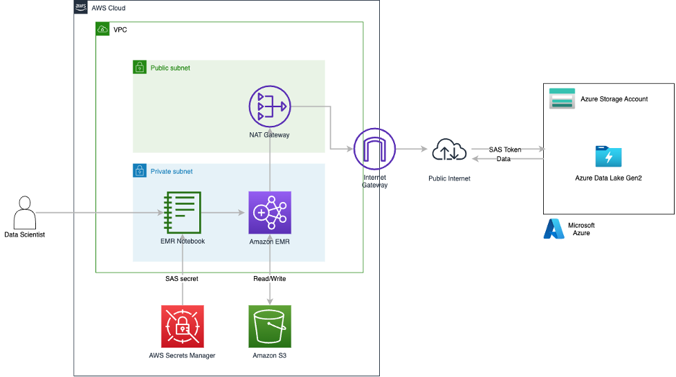
We walk through the following high-level steps to implement the solution:
For this setup, data is going over the public internet, which is not a best practice nor an AWS recommendation, but it’s sufficient to showcase the Amazon EMR configurations that enable remote reads from ADLS. Solutions such as AWS Direct Connect or AWS Site-to-Site VPN should be utilized to secure data traffic in enterprise deployments.
For an AWS Command Line Interface (AWS CLI)-based deployment example, refer to the appendix at the end of this post.
To get this solution working, we have a set of prerequisites for both AWS and Microsoft Azure:
We are following the best practice of using Azure AD credentials to create a user delegation SAS when applications need access to data storage using shared access signature tokens. In this post, we create and use a user delegation SAS with read and list permissions for ADLS access. For more information about creating SAS tokens using the Azure portal, refer to Use the Azure portal.
Before we generate the user delegation SAS token, we need to ensure the credential that will be used to generate the token has appropriate permissions to access data on the ADLS storage account. Requests submitted to the ADLS account using the user delegation SAS token are authorized with the Azure AD credentials that were used to create the SAS token.
The following minimum Azure role-based access control is required at the storage account level to access the data on ADLS storage:
To create the supported version of an EMR cluster with the required SAS configurations and stage all the required artifacts in Amazon S3, complete the following steps:
us-east-1).
As of this writing, the stack has been tested against 6.9.0 and 6.10.0.

S3ArtifactsBucket.emr-spark-on-adls-<GUID> to be redirected to the bucket on the Amazon S3 console.EMR/ folder.
artifacts/ folder.There are five artifacts staged by the CloudFormation stack in this path:
SASTokenProvider interface.azsastknprovider-1.0-SNAPSHOT.jar across cluster nodes.Medallion_Drivers_-_Active.csv and choose Download.EMR-Direct-Read-From-ADLS.ipynb and choose Download.To generate the user delegation SAS token from the Azure portal, log in to the Azure portal with your account credentials and complete the following steps:


Medallion_Drivers_-_Active.csv file downloaded earlier.Next, we secure the SAS token in Secrets Manager so it can be programmatically pulled from the Jupyter notebook.
us-east-1).

Setting up a secret rotation is a best practice but out of scope for this post. You can do so via Azure RM PowerShell, which can be integrated with the Lambda rotation function from Secrets Manager.

Finally, we create the EMR notebook environment, integrate the SAS token into the downloaded Jupyter notebook, and perform a read against ADLS.
us-east-1).
On the Summary tab, you will find the applications deployed on the cluster.

On the Configurations tab, you can see the configurations deployed by the CloudFormation stack loading the customer JAR in the appropriate classpaths.


EMR-Direct-Read-From-ADLS.ipynb notebook.EMR-Direct-Read-From-ADLS.ipynb from the left pane and ensure that the interpreter selected for the notebook in the top-right corner is PySpark.
SAS TOKEN SETUP markup cell, replace <AWS_REGION> with the Region you are using (in this case, us-east-1).You can get the secret key from Secrets Manager in the Secret value section for the secret you created earlier.

CONFIGURATIONS markup cell, replace <YOUR_STORAGE_ACCOUNT> with your Azure storage account where the SAS token was set up earlier.READ TEST DATA markup cell, replace <YOUR_CONTAINER> and <YOUR_STORAGE_ACCOUNT> with your Azure container and storage account name, respectively.
After all notebook cells run, you should see 10 rows in a tabular format containing the data coming from ADLS, which now can be used directly in the notebook or can be written to Amazon S3 for further use.

Deploying a CloudFormation template incurs cost based on the resources deployed. The EMR cluster is configured to stop after an hour of inactivity, but to avoid incurring ongoing charges and to fully clean up the environment, complete the following steps:
ElasticMapReduce-Master-Private, ElasticMapReduce-Slave-Private, ElasticMapReduce-ServiceAccess, ElasticMapReduceEditors-Livy, and ElasticMapReduceEditors-Editor security groups attached to the VPC created by the CloudFormation stack and delete their inbound and outbound rules.EMR_Notebooks_DefaultRole and choose Delete.In this post, we used AWS CloudFormation to deploy an EMR cluster with the appropriate configurations to connect to Azure Data Lake Storage using SAS tokens over the public internet. We provided an implementation of the SASTokenProvider interface to enable the SAS token-based connectivity to ADLS. We also provided relevant information on the SAS token creation steps on the Azure side. Furthermore, we showed how data scientists and analysts can use EMR notebooks connected to an EMR cluster to read data directly from ADLS with a minimum set of configurations. Finally, we used Secrets Manager to secure the storage of the SAS token and integrated it within the EMR notebook.
We encourage you to review the CloudFormation stack YAML template and test the setup on your own. If you implement the example and run into any issues or just have feedback, please leave a comment.
If you prefer to use command line options, this section provides AWS CLI commands to deploy this solution. Note that this is an alternative deployment model different from the CloudFormation template provided in the previous sections. Sample scripts and commands provided here include placeholders for values that need to be updated to suit your environment. The AWS CLI commands provided in this section should be used as guidance to understand the deployment model. Update the commands as needed to follow all the security procedures required by your organization.
The following are the assumptions made while using this AWS CLI-based deployment:
You must also complete additional requirements on the AWS and Azure sides.
For AWS, complete the following prerequisites:
For Azure, complete the following prerequisites:
We have created a custom class that implements the SASTokenProvider interface and created a JAR file called azsastknprovider-1.0-SNAPSHOT.jar, which is provided as a public artifact for this post. A set of configurations are required on the Amazon EMR side to use the SAS tokens to access ADLS. A sample configuration file in JSON format called EMR-HadoopSpark-ADLS-SASConfig.json is also provided as a public artifact for this post. Download the JAR and sample config files.
While copying the code or commands from this post, make sure to remove any control characters or extra newlines that may get added.
azsastknprovider-1.0-SNAPSHOT.jar (provided in this post) to the EMR cluster nodes’ local storage during the bootstrap phase. The following code is a sample bootstrap shell script:
EMR-HadoopSpark-ADLS-SASConfig.json locally in the same directory from where you plan to run the AWS CLI commands.We use the create-cluster command in the AWS CLI to deploy an EMR cluster. We need a bootstrap action at cluster creation to copy the custom JAR file to the EMR cluster nodes’ local storage. We also need to add a few custom configurations on Amazon EMR to connect to ADLS. For this, we need to supply a configuration file in JSON format. The following code launches and configures an EMR cluster that can connect to your Azure account and read objects in ADLS through Hadoop and Spark:
The following additional properties should be set inside your Spark application code to access data in ADLS through Amazon EMR. These should be set on the Spark session object used within your Spark application code.
These additional configurations can be set in the core-site.xml file for the EMR cluster. However, setting these in the application code is more secure and recommended because it won’t expose the SAS token in the Amazon EMR configurations.
You can run a Spark application on Amazon EMR in different ways:
To read files in ADLS within a Spark application that is running on an EMR cluster, you need to use the abfs driver and refer to the file in the following format, just as you would have done in your Azure environment:
The following sample PySpark script reads a CSV file in ADLS using SAS tokens and writes it to Amazon S3, and can be run from the EMR cluster you created:
Delete the EMR cluster created using the delete-cluster command.
 Kiran Anand is a Principal Solutions Architect with the AWS Data Lab. He is a seasoned professional with more than 20 years of experience in information technology. His areas of expertise are databases and big data solutions for data engineering and analytics. He enjoys music, watching movies, and traveling with his family.
 Andre Hass is a Sr. Solutions Architect with the AWS Data Lab. He has more than 20 years of experience in the databases and data analytics field. Andre enjoys camping, hiking, and exploring new places with his family on the weekends, or whenever he gets a chance. He also loves technology and electronic gadgets.
 Stefan Marinov is a Sr. Solutions Architecture Manager with the AWS Data Lab. He is passionate about big data solutions and distributed computing. Outside of work, he loves spending active time outdoors with his family.
 Hari Thatavarthy is a Senior Solutions Architect on the AWS Data Lab team. He helps customers design and build solutions in the data and analytics space. He believes in data democratization and loves to solve complex data processing-related problems.
 Hao Wang is a Senior Big Data Architect at AWS. Hao actively works with customers building large scale data platforms on AWS. He has a background as a software architect on implementing distributed software systems. In his spare time, he enjoys reading and outdoor activities with his family.
Post Syndicated from BeardedTinker original https://www.youtube.com/watch?v=z7blY6D-Qmk
Post Syndicated from Talks at Google original https://www.youtube.com/watch?v=EMe4sz1wn30