Tag Archives: Experience-Based Acceleration

Accelerating legacy code modernization: EPAM’s journey with Amazon Q Developer

Post Syndicated from Venugopalan Vasudevan original https://aws.amazon.com/blogs/devops/accelerating-legacy-code-modernization-epams-journey-with-amazon-q-developer/

This post is co-written with Nazariy Popov, Volodymyr Konchuk, and Andrii Davydenko from EPAM

Legacy code modernization presents significant challenges for organizations looking to stay competitive in today’s rapidly evolving digital landscape. Organizations face the dual challenge of maintaining business continuity while modernizing their legacy systems for cloud environments. This transformation requires organizations to carefully navigate between preserving essential business logic and implementing modern architectural patterns. This is where AI-powered development tools can make a transformative impact, as demonstrated in EPAM’s recent legacy modernization project using Amazon Q Developer.

Amazon Q Developer, an AI code assistant, seamlessly integrates into the development pipeline to address these challenges. This innovative AI code assistant helps teams tackle various tasks, from generating new features, automating language upgrades, and refactoring legacy code to fixing bugs and automating deployments. By providing detailed explanations for its code suggestions while maintaining high quality standards, Amazon Q Developer significantly improves developer efficiency across the entire software development lifecycle, resulting in substantial time and effort savings.

EPAM, an AWS Premier Partner, collaborated with one of their customers to modernize their legacy applications to AWS Cloud. The modernization initiative focused on multiple business-critical applications, primarily built in Java 8 with Oracle Database backend.

In this post, you’ll learn how Amazon Q Developer helped EPAM engineers transform these complex legacy systems into modern cloud-native architectures on AWS. The tool enabled the team to autonomously perform a range of tasks—from implementing new microservices and documenting code to testing, reviewing, and refactoring Java code, as well as performing critical platform upgrades.

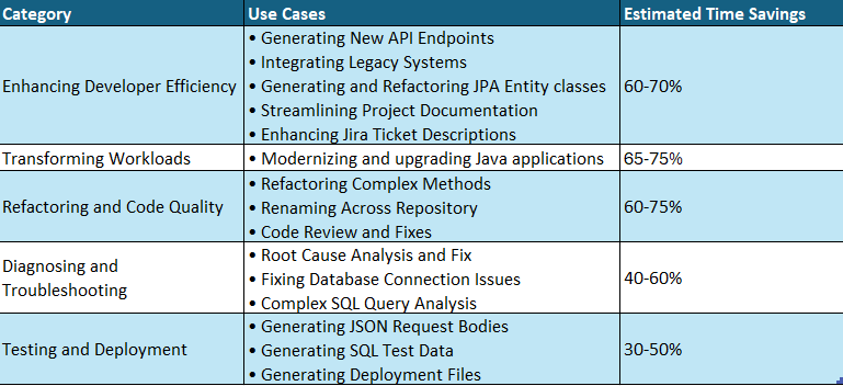
Before diving into the details, here’s an overview of how Amazon Q Developer helped EPAM across various aspects of the modernization project:

Summary of Amazon Q Developer Use Cases in EPAM’s Modernization Journey:

Summary of Amazon Q Developer Use Cases and Savings

Let’s explore each of these areas in detail.

Enhancing developer efficiency (Estimated time savings: 60-70%)

Amazon Q Developer played a crucial role in boosting EPAM’s development productivity. By automating routine tasks and providing intelligent code suggestions, the tool enabled developers to focus on more strategic aspects of the modernization project. Let’s explore how EPAM leveraged these capabilities.

Use Case 1: Generating New API Endpoints

Creating new API endpoints traditionally requires developers to invest 1-2 days per endpoint, involving multiple steps from designing the API contract to writing unit tests and documentation. Using Amazon Q Developer, the team dramatically accelerated this process for three new API endpoints in an existing microservice. Q Developer efficiently generated the initial code implementation along with comprehensive unit test coverage, requiring only minor modifications such as renaming variables, enhancing error handling, and refining test cases. The unit tests generated proved remarkably reliable with minimal adjustments needed. Along with this, Q Developer also generated comprehensive comments/documentation of the code improving the maintainability. This reduced the total development time to just 4 hours for all three endpoints – a 70% time saving compared to the traditional approach, allowing developers to focus on fine-tuning business logic rather than writing boilerplate code.

Use Case 2: Integrating Legacy Systems

Integrating a legacy monolith application with modern microservices traditionally requires developers to manually write extensive integration code, taking 1-2 weeks per integration point. Amazon Q Developer accelerated this process by automatically generating REST API client code in the monolith to consume microservice endpoints, along with data transfer objects (DTOs), error handling, and retry logic with integration test templates. While developers still needed to validate business rules and fine-tune error scenarios, Q Developer’s ability to understand both the legacy monolith’s structure and modern microservice patterns reduced the integration time to 2-3 days per integration point – a 70% time saving. This significantly streamlined the integration process while maintaining the robustness required for production systems.

Use Case 3: Generating and Refactoring JPA Entity Classes

During the modernization effort, new database tables were required to support additional business functionality in both the monolith and microservices. Instead of manually coding the data access layer, Amazon Q Developer automated the process by generating Spring JPA Entity classes from SQL DDL statements. Amazon Q Developer maintained consistency with existing data models by following established naming conventions, applying standard annotations, and implementing required interfaces from the existing codebase. What stood out was Q Developer’s ability to provide detailed explanations for its implementation choices, such as why specific annotations were used or how the new entities aligned with existing persistence patterns, enabling the team to quickly validate the generated code against their architectural standards. Amazon Q Developer generated the complete Java Spring entity class with all the fields. Additionally, Amazon Q Developer refactored the Entity class as well.

Use Case 4: Streamlining Project Documentation

Creating and maintaining up-to-date project documentation is often a time-consuming task for developers. Amazon Q Developer simplified this process by assisting in the generation of README files for the team’s projects. By analyzing the project structure, dependencies, and key components, Q Developer produced initial drafts of README files that included project overviews, setup instructions, and API documentation. This allowed developers to quickly review and refine the documentation, ensuring it met team standards while saving significant time compared to writing everything from scratch.

Use Case 5: Enhancing Jira Ticket Descriptions

Writing detailed, informative Jira ticket descriptions can be a challenge, especially for complex features or bug fixes. Amazon Q Developer aided the team by suggesting detailed descriptions for Jira tickets based on the context of the code changes and related discussions. For example, when creating a ticket for a new feature, Q Developer could propose a description that included the feature’s purpose, key implementation details, and potential impact on other system components. While developers still needed to review and adjust these descriptions, the AI-generated starting point significantly reduced the time spent on ticket management, allowing the team to focus more on actual development work.

Transforming workloads (Estimated time savings: 65-75%)

Moving legacy applications to the cloud requires careful planning and execution. EPAM utilized Amazon Q Developer’s Java upgrade capabilities to streamline the transformation of monolithic applications into modern, cloud-native architectures. Here’s how the Amazon Q Developer facilitated this process.

Use Case 6: Modernizing and upgrading Java applications

Amazon Q Developer assisted in upgrading older Java applications to Java 21 to leverage modern features like Java Streams API and adapting it for Spring Boot tech stack. It not only upgraded the code, but also updated deprecated code components, dependencies and libraries as well. This modernization improved the code’s performance and also aligned it with the current best practices adopted by the development teams. For large monolithic applications, breaking/decomposing the monolith into logical groups while identifying and separating common modules as shared dependencies helped break down the problem into manageable pieces for the agent to do a better job, resulting in a more maintainable and modular structure for the transformation process. This modular approach significantly enhanced Q Developer’s ability to analyze and transform the codebase while reducing the complexity of the modernization effort.

Refactoring Code, Improving Code Quality and Readability (Estimated time savings: 60-75%)

One of the most challenging aspects of modernization is refactoring legacy code and maintaining high code quality standards. Amazon Q Developer assisted EPAM’s team in analyzing complex codebases and suggesting improvements, optimizing the code while preserving business logic and ensuring consistent code quality. The following examples demonstrate this capability in action.

Use Case 7: Refactoring Complex Methods

Legacy code often includes methods with high cyclomatic complexity, making them difficult to maintain. Amazon Q Developer helped the development team refactor large, complex methods into smaller, more readable, and better-structured methods. It also provided a detailed explanation of the changes, highlighting how the refactored code improved maintainability and readability.

Use Case 8: Renaming Across the Repository

When tasked with renaming ‘YTD Tax Report‘ to ‘Withholding Tax Report‘ across the entire repository, Amazon Q Developer demonstrated capabilities beyond simple search and replace functionality found in traditional IDEs. It performed context-aware renaming, distinguishing between instances where ‘YTD Tax Report‘ was part of larger phrases or variable names, while simultaneously updating related components including unit tests, integration tests, and logging statements. The tool intelligently refactored method signatures where the report name was part of method names or parameters, analyzed and updated database queries, and maintained consistency across different file types including Java, XML, and properties files. What set Q Developer apart was its ability to provide detailed change logs explaining each modification and the rationale behind more complex refactoring decisions, significantly reducing the risk of missed references or inconsistencies that often occur with manual search-and-replace operations.

Use Case 9: Code Review and fixes

The code review capabilities of Amazon Q Developer, seamlessly integrated into the IDE, enabled the development team to detect potential issues spanning multiple classes. Beyond merely identifying problems, Q Developer provided actionable fix recommendations that could be easily reviewed and implemented. This proactive approach to code quality allowed the team to address issues during the early stages of development, significantly reducing the likelihood of defects making their way to production environments.

Diagnosing and troubleshooting errors (Estimated time savings: 40-60%)

Quick error resolution is crucial for maintaining development momentum. Amazon Q Developer’s advanced error analysis capabilities helped EPAM’s team identify and fix issues efficiently, reducing debugging time significantly. Here are some examples of how this worked in practice.

Use Case 10: Root Cause Analysis and Fix

During the development phase, the team encountered an unexpected error in one of the Java services: java.lang.IllegalArgumentException: Property 'http://javax.xml.XMLConstants/property/accessExternalDTD' is not recognized. Q Developer conducted a deeper analysis based on the context provided and suggested a more targeted fix and generated the necessary Java code changes, provided unit tests to verify the fix, and outlined potential security implications of the change. This comprehensive solution not only resolved the immediate error but also improved the overall security posture of the XML processing in the application. The team was able to implement and verify the fix within minutes, significantly reducing development.

Use Case 11: Fixing Database Connection Issues

While troubleshooting an issue where the application became unresponsive due to JDBC connection problems, Amazon Q Developer analyzed the project code and identified the missing connection pool configuration. Q Developer suggested implementing essential connection pool parameters like 'maximumPoolSize=20' and 'connectionTimeout=30000' based on the application’s traffic patterns and code. After implementing its suggested configuration, the issue was resolved, significantly improving the application’s stability.

Use Case 12: Complex SQL Query Analysis

Debugging complex SQL queries constructed dynamically in Java code can be challenging. Amazon Q Developer analyzed such queries, broke them down into their component parts, and provided descriptions for query parameters. For instance, when presented with a complex query involving multiple joins and subqueries, Q Developer dissected it into logical blocks, explaining how each part contributed to the overall result set. This made it easier for the team to understand and debug the queries.

Testing and Deployment: Test data generation and Automating Infrastructure Setup (Estimated time savings: 30-50%)

Use Case 13: Generating JSON Request Bodies

When testing new APIs, Amazon Q Developer generated JSON request bodies based on the corresponding Java classes. It provided detailed descriptions of each field and suggested realistic and meaningful default values, making it easier to validate API functionality with real-world scenarios.

Use Case 14: Generating SQL Test Data

Amazon Q Developer generated SQL insert statements with test data based on our existing Java Entity classes. This automation saved us a significant amount of time in creating realistic test data for database validation and integration testing.

Use Case 15: Generating Deployment Files

Amazon Q Developer helped the development team generate essential deployment artifacts, including a Docker file, a startup shell script that was used as an entry point, and a Kubernetes deployment file for a new service. Automating this process not only saves time but also improves consistency across environments.

Ready to transform your developer experience?

EPAM’s experience with Amazon Q Developer has been transformative, significantly accelerating their application modernization efforts while maintaining high code quality. By leveraging Amazon Q Developer, EPAM reduced development time by approximately 70% and improved code quality metrics across the client’s portfolio. This efficiency gains not only accelerated the client’s cloud migration timeline but also resulted in substantial cost savings and faster time-to-market for new features.

Now, it’s your turn to explore Amazon Q Developer:

Schedule a demo: Experience firsthand how Amazon Q Developer can accelerate your development lifecycle. Connect with our team for a personalized demonstration tailored to your specific use case.

Start Your Proof of Concept: Begin your journey with Amazon Q Developer today through a proof of concept. See how it can enhance your team’s productivity and code quality, just as it did for EPAM.

Connect with EPAM: Learn more about EPAM’s success story and best practices for implementing Amazon Q Developer in your organization’s development workflow.

Take the next step in revolutionizing your development process. Visit Amazon Q Developer website or contact your AWS account team to get started.

Authors

EPAM

Nazariy Popov (1) Nazariy Popov, Delivery Head of GenAI Engineering and Modernization Practice Delivery management professional and technology leader with over 15 years of experience in the IT industry. At EPAM, he drives large-scale transformation programs, focusing on enterprise software development, cloud solutions, and AI assisted engineering and modernization.
Volodymyr Konchuk Volodymyr Konchuk, Lead Software Engineer
Java engineer with more than 11 years of production experience in Java-based web and enterprise applications. Has experience in building ecommerce and retail business applications using Java, Spring tech stack, and Amazon Web Services.
Andriy Davydenko

Andrii Davydenko, Delivery Manager
Seasoned delivery lead with over 7 years of experience managing ecommerce modernization projects with a focus on application performance optimization.

AWS

Venugopalan Vasudevan (Venu) is a Senior Specialist Solutions Architect focusing on Next Generation Developer Experience and AWS Generative AI services. In this role, Venu, helps organizations optimize their development processes and accelerate their digital transformation journeys using Amazon Q Developer and other AWS Generative AI Services. Also, Venu partners with enterprises to architect and implement Generative AI solutions while establishing robust development practices.
ArunChandapillai Arun Chandapillai is a Senior Engineering Architect with a strong history of leading cross-functional teams and collaborating with executive stakeholders. He is passionate about helping customers accelerate IT modernization through business-first cloud adoption strategies, with a focus on leveraging generative AI and MLOps. Outside of technology, he is an automotive enthusiast who loves the thrill of the open road, an engaging public speaker, and a philanthropist who lives by the motto ‘you get (back) what you give’.
jasmine Jasmine Rasheed Syed is a Senior Customer Solutions manager, focused in accelerating time to value for the customers in their in cloud journey by adopting best practices and mechanisms to transform their business at scale. Jasmine is a seasoned, result oriented leader with 20+ years of progressive experience in Insurance, Retail & CPG with exemplary track record spanning across Business Development, Cloud/Digital Transformation, Delivery, Operational & Process Excellence and Executive Management.
Oscar Oscar Hernandez is a Senior Account Executive, helping global organizations drive digital and AI transformation at scale. He works closely with executive teams to integrate cloud and AI-driven solutions that address complex business challenges and deliver measurable enterprise-wide impact. With over 15 years of experience across IT, telecom, financial services, retail, and HR technology, he focuses on enabling innovation, optimizing operations, and maximizing the value of emerging technologies.

How Stifel built a modern data platform using AWS Glue and an event-driven domain architecture

Post Syndicated from Amit Maindola original https://aws.amazon.com/blogs/big-data/how-stifel-built-a-modern-data-platform-using-aws-glue-and-an-event-driven-domain-architecture/

Stifel Financial Corp. is an American multinational independent investment bank and financial services company, founded in 1890 and headquartered in downtown St. Louis, Missouri. Stifel offers securities-related financial services in the United States and Europe through several wholly owned subsidiaries. Stifel provides both equity and fixed income research and is the largest provider of US equity research.

In this post, we show you how Stifel implemented a modern data platform using AWS services and open data standards, building an event-driven architecture for domain data products while centralizing the metadata to facilitate discovery and sharing of data products.

Stifel’s modern data platform use case

Stifel envisioned a data platform that delivers accurate, timely, and properly governed data, providing consistency throughout the organization whenever users access the information. This approach showed limitations as the data complexity increased, data volumes grew, and demand for quick, business-driven insights rose. These challenges are encountered by financial institutions worldwide, leading to a reassessment of traditional data management practices. Under the federated governance model, Stifel developed a modern data strategy based on the following objectives:

  • Managing ingestion and metadata
  • Creating source-aligned data products complying with Stifel business streams
  • Integrating source-aligned data products from other domains (Stifel business units)
  • Producing consumer-aligned data products for specific business purposes
  • Publishing data products to a centralized data catalog

Some of the Stifel challenges highlighted in the preceding list required building a data platform that can:

  • Boost agility by democratizing data, thus reducing time to market and enhancing the customer experience
  • Improve data quality and trust in the data
  • Standardize tools and eliminate the shadow information technology (IT) culture to increase scalability, reduce risk, and minimize operational inefficiencies

Following the federated governance model, Stifel has organized its domain structure to provide autonomy to various functional teams while preserving the core values of data mesh. The following diagram depicts a high-level architecture of the data mesh implementation at Stifel.

Each data domain has the flexibility to create data products that can be published to the centralized catalog, while maintaining the autonomy for teams to develop data products that are exclusively accessible to teams within the domain. These products aren’t available to others until they are deemed ready for broader enterprise use. Domains have the freedom to decide which data they want to share. They can either:

  • Make their data products visible to everyone through the central catalog
  • Keep their data products visible only within their own domain

By implementing an event-driven domain architecture, organizations can achieve significant business advantages while positioning themselves for future growth and innovation. Stifel data products refreshes were dependent on data assets with variable cadence. Event-driven architecture enables real-time or near real-time updates by allowing data products to automatically respond to changes in underlying data assets as they occur, rather than relying on fixed batch schedules that might miss critical updates or waste resources on unnecessary refreshes. The key is to carefully plan the implementation and make sure of alignment with business objectives while considering both technical and organizational factors. This architecture style particularly suits organizations that:

  • Need real-time processing capabilities
  • Have complex domain interactions
  • Require high scalability
  • Want to improve business agility
  • Need better system integration
  • Are pursuing digital transformation

The following are some of the key AWS Services that helped Stifel to build their modern data platform.

  • AWS Glue is a serverless data integration service that’s used for data processing to build data assets and data products in the domains. Data is also cataloged in AWS Glue Catalog, making it straightforward to discover and query with supported engines.
  • Amazon EventBridge provides a scalable and flexible serverless event bus that facilitates seamless communication between different domains and services. By using EventBridge, Stifel was able to implement a publish-subscribe model where domain events can be emitted, filtered, and routed to appropriate consumers based on configurable rules. EventBridge supports custom event buses for domain-specific events, enabling clear separation of concerns and improved manageability.
  • AWS Lake Formation helped in providing centralized security, governance, and catalog capabilities while preserving domain autonomy in data product creation and management. With Lake Formation, data domains were able to maintain their independent data products within a federated structure while enforcing consistent access controls, data quality standards, and metadata management across the organization.
  • Apache Hudi on Amazon Simple Storage Service (Amazon S3) offers an optimized way to store data assets and products and promotes interoperability across other services.

Stifel’s solution architecture

The following diagram illustrates the data mesh architecture that Stifel uses to build a domain-driven architecture. In this system, various domains create data products and share them with other domains through a central governance account that uses Lake Formation.

Let’s look at some of the key design components that are being used to enable and implement data mesh and event driven design

Data ingestion framework

The data ingestion framework consists of several processor modules that are built using several AWS services and metadata driven architecture. The following diagram shows the architecture of the raw data ingestion framework.

The framework gets raw data files from both internal Stifel systems and third-party data sources. These files are processed and stored in a raw data ingestion account on Amazon S3 in open table format Apache Hudi. This stored data is then shared with different parts of the organization, called data domains. Each domain can use this shared data to create their own data products.

As a file (in CSV, XML, JSON and custom formats) lands into the landing bucket, an Amazon S3 event notification is created and placed in an Amazon Simple Queue Service (Amazon SQS)queue. The Amazon SQS queue triggers an AWS Lambda function and saves the metadata (such as the name of the file, date and time the file was received, and the file size) to a file audit data store (Amazon Aurora PostgreSQL-Compatible Edition).

An EventBridge time scheduler invokes an AWS Step Functions workflow at pre-determined intervals. The Step Functions workflow orchestrates the batch ingestion from raw to staging layer.

  1. The Step Functions workflow orchestrates a set of Lambda functions to get the list of unprocessed raw files from the audit data store and create batches of raw files to process them in parallel. The Step Functions workflow then triggers parallel AWS Glue jobs that process each batch of raw files.
  2. Each raw file is validated for any data quality checks and the data is saved to staging tables in Hudi format. Any errors encountered are logged into an audit table and a notification is generated for support team. For all successfully processed raw files, the file status is updated to PROCESSED and logged into an audit table.
  3. After the Hudi table is updated, a data refresh event is sent to EventBridge and then passed to the Central Mesh Account. The Central Mesh Account forwards these events to the data domains to notify them that the raw tables are refreshed, allowing the data domains to use this data for creating their own data products.

Event driven data product refresh

The Stifel data lake is based on a data mesh architecture where several data producers share data across data domains. A mechanism is needed to alert consumers who depend on other data producers’ data products when those source data products are refreshed, so that the consumers can update their own data products accordingly. The following diagram describes the technical architecture of event-based data processing. The central governance account acts as the central event bus, which receives all data refresh events from all data producers. The central event bus forwards the events to consumer accounts. The consumer accounts filter the events consumers are interested in from data producers for their data processing needs.

Orchestration design

Stifel designed and implemented an event-based data pipeline orchestration system that triggers data pipelines when specific events occur. This system processes data immediately after receiving all required dependency events, enabling efficient workflow management.

The following diagram describes the logical architecture of the domain data pipeline orchestration framework.

The orchestration framework includes the components described in the following list. The data dependencies and data pipeline state management metadata are hosted in an Aurora PostgreSQL database.

  1. Data refresh processor: Receives data refresh events from central mesh and local data domain and evaluates if the domain data products data dependencies are met
  2. Data product dependency processor: Retrieves metadata for the product, kicks off a corresponding data domain AWS Glue job, and updates metadata with the job information
  3. Data pipeline state change processor: Monitors the domain data jobs and takes actions based on the job’s final status (SUCCEED or FAILED) and then creates incident tickets for failed jobs

Conclusion

Stifel has improved its data management and reduced data silos by adopting a data product approach. This strategy has positioned Stifel to become a data-driven, customer-centric organization. The company combines federated platform practices with AWS and open standards. As a result, Stifel is achieving its decentralization objectives through a scalable data platform. This platform empowers domain teams to make informed decisions, drive innovation, and maintain a competitive edge. Here are the some of the advantages Stifel got from an event-driven domain architecture (EDDA):

  • Business agility: Rapid market response, new business capability integration, scalable domains, quicker feature deployment, and flexible process modification
  • Customer experience: Real-time processing, responsive interactions, personalized services, consistent omnichannel presence, and enhanced service availability
  • Operational efficiency: Reduced system coupling, optimal resource use, scalable systems, lower maintenance overhead, and efficient data processing
  • Cost benefits: Lower development costs, reduced infrastructure expenses, decreased maintenance costs, efficient resource usage, and a better ROI on technology investments

In this post, we demonstrated how Stifel is building a modern data platform by recognizing the critical importance of data in today’s financial landscape. This strategic approach not only enhances operational efficiency but also positions Stifel at the forefront of technological innovation in the financial services industry. To learn more and get started, see the following resources:


About the authors

Amit Maindola is a Senior Data Architect focused on data engineering, analytics, and AI/ML at Amazon Web Services. He helps customers in their digital transformation journey and enables them to build highly scalable, robust, and secure cloud-based analytical solutions on AWS to gain timely insights and make critical business decisions.

Srinivas Kandi is a Senior Architect at Stifel focusing on delivering the next generation of cloud data platform on AWS. Prior to joining Stifel, Srini was a delivery specialist in cloud data analytics at AWS helping several customers in their transformational journey into AWS cloud. In his free time, Srini likes to explore cooking, travel and learn new trends and innovations in AI and cloud computing.

Hossein Johari is a seasoned data and analytics leader with over 25 years of experience architecting enterprise-scale platforms. As Lead and Senior Architect at Stifel Financial Corp. in St. Louis, Missouri, he spearheads initiatives in Data Platforms and Strategic Solutions, driving the design and implementation of innovative frameworks that support enterprise-wide analytics, strategic decision-making, and digital transformation. Known for aligning technical vision with business objectives, he works closely with cross-functional teams to deliver scalable, forward-looking solutions that advance organizational agility and performance.

Ahmad Rawashdeh is a Senior Architect at Stifel Financial. He supports Stifel and its clients in designing, implementing, and building scalable and reliable data architectures on Amazon Web Services (AWS), with a strong focus on data lake strategies, database services, and efficient data ingestion and transformation pipelines.

Lei Meng is a data architect at Stifel. His focus is working in designing and implementing scalable and secure data solutions on the AWS and helping Stifel’s cloud migration from on-premises systems.

How Skroutz handles real-time schema evolution in Amazon Redshift with Debezium

Post Syndicated from Konstantina Mavrodimitraki original https://aws.amazon.com/blogs/big-data/how-skroutz-handles-real-time-schema-evolution-in-amazon-redshift-with-debezium/

This guest post was co-authored with Kostas Diamantis from Skroutz.

At Skroutz, we are passionate about our product, and it is always our top priority. We are constantly working to improve and evolve it, supported by a large and talented team of software engineers. Our product’s continuous innovation and evolution lead to frequent updates, often necessitating changes and additions to the schemas of our operational databases.

When we decided to build our own data platform to meet our data needs, such as supporting reporting, business intelligence (BI), and decision-making, the main challenge—and also a strict requirement—was to make sure it wouldn’t block or delay our product development.

We chose Amazon Redshift to promote data democratization, empowering teams across the organization with seamless access to data, enabling faster insights and more informed decision-making. This choice supports a culture of transparency and collaboration, as data becomes readily available for analysis and innovation across all departments.

However, keeping up with schema changes from our operational databases, while updating the data warehouse without constantly coordinating with development teams, delaying releases, or risking data loss, became a new challenge for us.

In this post, we share how we handled real-time schema evolution in Amazon Redshift with Debezium.

Solution overview

Most of our data resides in our operational databases, such as MariaDB and MongoDB. Our approach involves using the change data capture (CDC) technique, which automatically handles the schema evolution of the data stores being captured. For this, we used Debezium along with a Kafka cluster. This solution enables schema changes to be propagated without disrupting the Kafka consumers.

However, handling schema evolution in Amazon Redshift became a bottleneck, prompting us to develop a strategy to address this challenge. It’s important to note that, in our case, changes in our operational databases primarily involve adding new columns rather than breaking changes like altering data types. Therefore, we have implemented a semi-manual process to resolve this issue, along with a mandatory alerting mechanism to notify us of any schema changes. This two-step process consists of handling schema evolution in real time and handling data updates in an asynchronous manual step. The following architectural diagram illustrates a hybrid deployment model, integrating both on-premises and cloud-based components.

End-to-end data migration workflow from on-premises databases to AWS cloud using CDC, messaging, and data warehouse services

The data flow begins with data from MariaDB and MongoDB, captured using Debezium for CDC in near real-time mode. The captured data is streamed to a Kafka cluster, where Kafka consumers (built on the Ruby Karafka framework) read and write them to the staging area, either in Amazon Redshift or Amazon Simple Storage Service (Amazon S3). From the staging area, DataLoaders promote the data to production tables in Amazon Redshift. At this stage, we apply the slowly changing dimension (SCD) concept to these tables, using Type 7 for most of them.

In data warehousing, an SCD is a dimension that stores data, and though it’s generally stable, it might change over time. Various methodologies address the complexities of SCD management. SCD Type 7 places both the surrogate key and the natural key into the fact table. This allows the user to select the appropriate dimension records based on:

  • The primary effective date on the fact record
  • The most recent or current information
  • Other dates associated with the fact record

Afterwards, analytical jobs are run to create reporting tables, enabling BI and reporting processes. The following diagram provides an example of the data modeling process from a staging table to a production table.

Database schema evolution: staging.shops to production.shops with added temporal and versioning columns

The architecture depicted in the diagram shows only our CDC pipeline, which fetches data from our operational databases and doesn’t include other pipelines, such as those for fetching data through APIs, scheduled batch processes, and many more. Also note that our convention is that dw_* columns are used to catch SCD metadata information and other metadata in general. In the following sections, we discuss the key components of the solution in more detail.

Real-time workflow

For the schema evolution part, we focus on the column dw_md_missing_data, which captures schema evolution changes in near real time that occur in the source databases. When a new change is produced to the Kafka cluster, the Kafka consumer is responsible for writing this change to the staging table in Amazon Redshift. For example, a message produced by Debezium to the Kafka cluster will have the following structure when a new shop entity is created:

{
  "before": null,
  "after": {
    "id": 1,
    "name": "shop1",
    "state": "hidden"
  },
  "source": {
    ...
    "ts_ms": "1704114000000",
    ...
  },
  "op": "c",
  ...
}

The Kafka consumer is responsible for preparing and executing the SQL INSERT statement:

INSERT INTO staging.shops (
  id,
  "name",
  state,
  dw_md_changed_at,
  dw_md_operation,
  dw_md_missing_data
)
VALUES
  (
    1,
    'shop1',
    'hidden',
    '2024-01-01 13:00:00',
    'create',
    NULL
  )
;

After that, let’s say a new column is added to the source table called new_column, with the value new_value.
The new message produced to the Kafka cluster will have the following format:

{
  "before": { ... },
  "after": {
    "id": 1,
    "name": "shop1",
    "state": "hidden",
    "new_column": "new_value"
  },
  "source": {
    ...
    "ts_ms": "1704121200000"
    ...
  },
  "op": "u"
  ...
}

Now the SQL INSERT statement executed by the Kafka consumer will be as follows:

INSERT INTO staging.shops (
  id,
  "name",
  state,
  dw_md_changed_at,
  dw_md_operation,
  dw_md_missing_data
)
VALUES
  (
    1,
    'shop1',
    'hidden',
    '2024-01-01 15:00:00',
    'update',
    JSON_PARSE('{"new_column": "new_value"}') /* <-- check this */
  )
;

The consumer performs an INSERT as it would for the known schema, and anything new is added to the dw_md_missing_data column as key-value JSON. After the data is promoted from the staging table to the production table, it will have the following structure.

Production.shops table displaying temporal data versioning with creation, update history, and current state indicators

At this point, the data flow continues running without any data loss or the need for communication with teams responsible for maintaining the schema in the operational databases. However, this data might not be easily accessible for the data consumers, analysts, or other personas. It’s worth noting that dw_md_missing_data is defined as a column of the SUPER data type, which was introduced in Amazon Redshift to store semistructured data or documents as values.

Monitoring mechanism

To track new columns added to a table, we have a scheduled process that runs weekly. This process checks for tables in Amazon Redshift with values in the dw_md_missing_data column and generates a list of tables requiring manual action to make this data available through a structured schema. A notification is then sent to the team.

Manual remediation steps

In the aforementioned example, the manual steps to make this column available would be:

  1. Add the new columns to both staging and production tables:
ALTER TABLE staging.shops ADD COLUMN new_column varchar(255);
ALTER TABLE production.shops ADD COLUMN new_column varchar(255);
  1. Update the Kafka consumer’s known schema. In this step, we just need to add the new column name to a simple array list. For example:
class ShopsConsumer < ApplicationConsumer
  SOURCE_COLUMNS = [
    'id',
    'name',
    'state',
    'new_column' # this one is the new column
  ]
 
  def consume
    # Ruby code for:
    #   1. data cleaning
    #   2. data transformation
    #   3. preparation of the SQL INSERT statement
 
    RedshiftClient.conn.exec <<~SQL
      /*
        generated SQL INSERT statement
      */
    SQL
  end
end
  1. Update the DataLoader’s SQL logic for the new column. A DataLoader is responsible for promoting the data from the staging area to the production table.
class DataLoader::ShopsTable < DataLoader::Base
  class << self
    def load
      RedshiftClient.conn.exec <<~SQL
        CREATE TABLE staging.shops_new (LIKE staging.shops);
      SQL
 
      RedshiftClient.conn.exec <<~SQL
        /*
          We move the data to a new table because in staging.shops
          the Kafka consumer will continue add new rows
        */
        ALTER TABLE staging.shops_new APPEND FROM staging.shops;
      SQL
 
      RedshiftClient.conn.exec <<~SQL
        BEGIN;
          /*
            SQL to handle
              * data deduplications etc
              * more transformations
              * all the necessary operations in order to apply the data modeling we need for this table
          */
 
          INSERT INTO production.shops (
            id,
            name,
            state,
            new_column, /* --> this one is the new column <-- */
            dw_start_date,
            dw_end_date,
            dw_current,
            dw_md_changed_at,
            dw_md_operation,
            dw_md_missing_data
          )
          SELECT
            id,
            name,
            state,
            new_column, /* --> this one is the new column <-- */
            /*
              here is the logic to apply the data modeling (type 1,2,3,4...7)
            */
          FROM
            staging.shops_new
          ;
 
          DROP TABLE staging.shops_new;
        END TRANSACTION;
      SQL
    end
  end
end
  1. Transfer the data that has been loaded in the meantime from the dw_md_missing_data SUPER column to the newly added column and then clean up. In this step, we just need to run a data migration like the following:
BEGIN;
 
  /*
    Transfer the data from the `dw_md_missing_data` to the corresponding column
  */
  UPDATE production.shops
  SET new_column = dw_md_missing_data.new_column::varchar(255)
  WHERE dw_md_missing_data.new_column IS NOT NULL;
 
  /*
    Clean up dw_md_missing_data column
  */
  UPDATE production.shops
  SET dw_md_missing_data = NULL
  WHERE dw_md_missing_data IS NOT NULL;
 
END TRANSACTION;

To perform the preceding operations, we make sure that no one else performs changes to the production.shops table because we want no new data to be added to the dw_md_missing_data column.

Conclusion

The solution discussed in this post enabled Skroutz to manage schema evolution in operational databases while seamlessly updating the data warehouse. This alleviated the need for constant development team coordination and removed risks of data loss during releases, ultimately fostering innovation rather than stifling it.

As the migration of Skroutz to the AWS Cloud approaches, discussions are underway on how the current architecture can be adapted to align more closely with AWS-centered principles. To that end, one of the changes being considered is Amazon Redshift streaming ingestion from Amazon Managed Streaming for Apache Kafka (Amazon MSK) or open source Kafka, which will make it possible for Skroutz to process large volumes of streaming data from multiple sources with low latency and high throughput to derive insights in seconds.

If you face similar challenges, discuss with an AWS representative and work backward from your use case to provide the most suitable solution.


About the authors

Konstantina Mavrodimitraki is a Senior Solutions Architect at Amazon Web Services, where she assists customers in designing scalable, robust, and secure systems in global markets. With deep expertise in data strategy, data warehousing, and big data systems, she helps organizations transform their data landscapes. A passionate technologist and people person, Konstantina loves exploring emerging technologies and supports the local tech communities. Additionally, she enjoys reading books and playing with her dog.

Kostas Diamantis is the Head of the Data Warehouse at Skroutz company. With a background in software engineering, he transitioned into data engineering, using his technical expertise to build scalable data solutions. Passionate about data-driven decision-making, he focuses on optimizing data pipelines, enhancing analytics capabilities, and driving business insights.

Streamline Operational Troubleshooting with Amazon Q Developer CLI

Post Syndicated from Kirankumar Chandrashekar original https://aws.amazon.com/blogs/devops/streamline-operational-troubleshooting-with-amazon-q-developer-cli/

Amazon Q Developer is the most capable generative AI–powered assistant for software development, helping developers perform complex workflows. Amazon Q Developer command-line interface (CLI) combines conversational AI with direct access to AWS services, helping you understand, build, and operate applications more effectively. The Amazon Q Developer CLI executes commands, analyzes outputs, and provides contextual recommendations based on best practices for troubleshooting tools and platforms available on your local machine.

In today’s cloud-native environments, troubleshooting production issues often involves juggling multiple terminal windows, parsing through extensive log files, and navigating numerous AWS console pages. This constant context-switching delays problem resolution and adds cognitive burden to teams managing cloud infrastructure.

In this blog post, you will explore how Amazon Q Developer CLI transforms the troubleshooting experience by streamlining challenging scenarios through conversational interactions.

The Traditional Troubleshooting Experience

When issues arise, engineers typically spend hours manually examining infrastructure configurations, reviewing logs across services, and analyzing error patterns. The process requires switching between multiple interfaces, correlating information from various sources, and deep AWS knowledge. This complex workflow often extends problem resolution from hours into days and increase the burden on the infrastructure teams.

Solution: Amazon Q Developer CLI

Amazon Q Developer CLI streamlines the entire troubleshooting process, from initial investigation to problem resolution, making complex AWS troubleshooting accessible and efficient through simple conversations.

How Amazon Q Developer CLI works:

  • Natural Language Interface: Execute AWS CLI commands and interact with AWS services using conversational prompts
  • Automated Discovery: Map out infrastructure and analyze configurations
  • Intelligent Log Analysis: Parse, correlate, and analyze logs across services
  • Root Cause Identification: Pinpoint issues through AI-powered reasoning
  • Guided Remediation: Implement fixes with minimal human intervention
  • Validation: Test solutions and explain complex issues simply

One of the built-in tools within the Amazon Q Developer CLI, use_aws, enables natural language interaction with AWS services, as shown in Figure 1. This tool leverages the AWS CLI permissions configured on your local machine, allowing secure and authorized access to your AWS resources.

A command line interface showing a list of tools and their permissions. The display is titled "/tools" and shows several built-in tools including execute_bash, fs_read, fs_write, report_issue, and use_aws. Each tool has an associated permission level indicated by asterisks. The use_aws tool is highlighted with "trust read-only commands" permission. At the bottom, there's a note stating "Trusted tools will run without confirmation" and a tip to "Use /tools help to edit permissions".

Figure 1: Tools selection in Amazon Q Developer CLI

Real-World Troubleshooting Scenario

Demonstration Environment Setup

This demonstration was performed with the following environment configuration:

The environment includes a local development machine with necessary tools, appropriate AWS account permissions, and terminal access. By starting Amazon Q Developer CLI in the project directory, it has immediate access to relevant code and configuration files.

Scenario: Troubleshooting NGINX 5XX Errors

The scenario demonstrates troubleshooting a multi-tier application architecture as shown in figure 2 deployed on Amazon ECS Fargate with:

  • Application Load Balancer (ALB) distributing traffic across availability zones
  • NGINX reverse proxy service handling incoming requests
  • Node.js backend service processing business logic
  • Service discovery enabling internal communication
  • CloudWatch Logs providing centralized logging

An AWS cloud architecture diagram showing the flow of traffic from an Internet user through multiple components. The diagram includes: At the top: An Internet user connecting to an Internet Gateway Within a VPC (Virtual Private Cloud): Two public subnets containing a NAT Gateway and Application Load Balancer Two private subnets within an ECS Cluster containing: An NGINX service (Fargate) A Backend service (Fargate) A 10-second timeout between them A Cloud Map Service Discovery component at the bottom CloudWatch Logs integration on the right side The diagram includes a note about gateway timeouts: "504 Gateway Timeout - Backend takes 15s to respond, NGINX timeout is 10s" All components are connected with arrows showing the flow of traffic and data through the system. The infrastructure follows AWS best practices with public and private subnet separation for security.

Figure 2: AWS Architecture diagram for the app used in this blog post

Traditional Troubleshooting Steps

For the architecture in figure 2, when 502 Gateway Timeout errors occur, traditional troubleshooting requires:

  1. Checking ALB target group health
  2. Examining ECS service status across multiple consoles
  3. Analyzing CloudWatch logs from different log groups
  4. Correlating error patterns between services
  5. Reviewing infrastructure code for configuration issues
  6. Implementing and deploying fixes

Amazon Q Developer CLI Approach

Instead, let’s see how Amazon Q Developer CLI handles this systematically, step by step:

Step1: Initial Problem Report

Amazon Q Developer CLI is provided with the initial prompt as a problem statement within the application project directory as shown in the following screenshot in figure 3. Amazon Q Developer responds back and says it is going investigate the 502 Gateway Timeout errors in the NGINX application.

Prompt:

Our production NGINX application is experiencing 502 Gateway Timeout errors. 
I have checked out the application and infrastructure code locally and the AWS CLI 
profile 'demo-profile' is configured with access to the AWS account where the 
infrastructure and application is deployed to. Can you help investigate and diagnose the issue?

A Visual Studio Code window showing a debugging session for an NGINX application. The interface has three main sections: a file explorer on the left showing project files including 'app.ts' and 'nginx-config-task.json', a terminal tab in the center displaying an "Amazon Q" ASCII art logo, and a conversation where a user is reporting 502 Gateway Timeout errors. The terminal shows AWS CLI command execution using a tool called "use_aws" with parameters including the service name "ecs" and region "us-west-2". The interface has red annotations highlighting key areas like "project files", "User provided initial prompt", and "Q CLI executing AWS CLI calls.

Figure 3: Amazon Q Developer CLI with initial prompt and problem statement

Step2: Systematic Infrastructure Discovery

Amazon Q Developer CLI start to systematically discovering the infrastructure as shown in the following screenshot in figure 4. If you see the initial prompt did not include that the app is hosted on ECS, but Amazon Q Developer CLI understood the context and executes the AWS CLI calls to describe the Cluster and the services within it. It made sure that the ECS tasks are running for both the services within the Cluster. It is a key discovery that both services show healthy status (1/1 desired count), indicating the issue isn’t service availability.

A terminal window showing three sequential AWS CLI commands being executed through a "use_aws" tool: First command: "list-clusters" operation for ECS service in us-west-2 region using demo-profile, completing in 1.244 seconds Second command: "list-services" operation targeting the NginxSimulationCluster, completing in 0.877 seconds with confirmation of finding both nginx-service and backend-service Third command: "describe-services" operation examining both services in detail, completing in 0.968 seconds with confirmation that both services are running as expected (1/1 desired count) Each command includes execution details, parameters, and completion status, with the system preparing to check CloudWatch logs next.

Figure 4: AWS Infrastructure discovery by Amazon Q Developer CLI

Step 3: Intelligent Log Analysis

Amazon Q Developer CLI retrieves and analyzes recent CloudWatch logs from the NGINX container, immediately identifying the critical error pattern as shown in the following screenshot in figure 5, where Amazon Q Developer responds: “Perfect! I found the issue. The NGINX logs show clear 504 gateway timeout with upstream timeout messages.”

A terminal window showing two AWS CloudWatch Logs commands being executed: First command: "describe-log-streams" operation for the "/ecs/nginx-service" log group, limiting to 5 most recent entries, ordered by LastEventTime in descending order Second command: "get-log-events" operation retrieving 50 log entries from a specific NGINX container log stream The output reveals a critical error message highlighted at the bottom showing an upstream timeout (error 110) occurring while reading response headers. The error details include client IP 10.0.0.247, upstream server at http://10.0.3.18:3000/, and host 52.35.62.210.

Figure 5: CloudWatch Log analysis by Amazon Q Developer CLI

Step 4: Amazon Q Developer CLI Analysis and Root Cause Identification

Amazon Q Developer examines backend service logs and discovers a mismatch between the backend service response time and NGINX timeout settings, as seen in the following screenshot in figure 6.

A terminal window showing AWS CloudWatch Logs commands and their output. The first command describes log streams for a backend container, and the second retrieves log events. The output reveals a debugging analysis showing that while health checks work fine, regular requests are being delayed by about 15 seconds, causing NGINX timeout issues. The log group is "/ecs/backend-service" in the us-west-2 region using a demo-profile.

Figure 6: Root cause identification by Amazon Q Developer CLI

Step 5: Amazon Q Developer CLI Root Cause Analysis

Amazon Q Developer CLI examines the ECS task definitions to identify the exact configuration mismatch, as shown in the following screenshot in figure 7. Amazon Q Developer finds that:

  • Backend service is configured with response_delay=15000 (15 secs)
  • NGINX proxy is configured with proxy_read_timeout 10s

This mismatch causes 504 gateway timeout errors when the backend response exceeds NGINX’s timeout threshold.

A terminal window showing two AWS CLI commands to describe ECS task definitions in the us-west-2 region. Below the commands is a highlighted "Root Cause Analysis" section that explains a timeout mismatch: the backend service is configured with a 15-second response delay while NGINX has a 10-second proxy timeout, resulting in 502 Gateway Timeout errors. Both commands use a demo-profile and are labeled as checking timeout and response delay configurations.

Figure 7: Root cause analysis and issue detection by Amazon Q Developer CLI

Step 6: Automated Code Fix

Here’s where Amazon Q Developer CLI truly excels—it doesn’t just diagnose; it implements the fix. Since Amazon Q Developer CLI is started within the project where the CDK code for ECS task definition is defined, it identified the code configuration and also modified it, as shown in the following screenshot in figure 8.

A terminal window showing file operations using fs_read and fs_write tools. The code changes show an NGINX configuration update in ecs-nginx-cdk.ts, where the proxy_read_timeout is being modified from '10s' to '20s'. The file also shows additional timeout configurations being added, including proxy_connect_timeout and proxy_send_timeout. The update is confirmed with a user prompt and completed in 0.2 seconds.

Figure 8: CDK code fix by Amazon Q Developer CLI

Step 7: Deployment

Amazon Q Developer CLI builds and deploys the fix by executing cdk synth and cdk deploy using the ‘demo-profile‘ AWS CLI profile that was initially provided in the prompt, as shown in the following screenshot in figure 9.

A terminal window showing two execute_bash commands running in sequence. The first command builds a CDK project using 'npm run build' in the nginx-app directory, completing in 4.102s. The second command deploys the updated CDK stack using 'cdk deploy' with the demo-profile, showing deployment progress including some warnings about minHealthyPercent configurations and CloudFormation stack updates in us-west-2 region.

Figure 9: CDK code build and deployment by Amazon Q Developer CLI

Step 8: Validation

Amazon Q Developer CLI validates the solution by sending a curl request to the ALB endpoint after the successful deployment, as shown in the following screenshot in figure 10.

A terminal window showing the execution of a curl command to test an NGINX application on AWS. The command targets an Elastic Load Balancer in the us-west-2 region. The response shows a successful HTTP 200 OK status after 14 seconds, with a JSON response containing the message "Hello from backend". The test completes in 15.100 seconds, indicating the fix for previous 502 errors was successful.

Figure 10: Fix validation by Amazon Q Developer CLI

In addition to that, Amazon Q Developer also sends a request to the health check endpoint and validates everything is working after the fix was deployed, as shown in the following screenshot in figure 11.

A terminal screenshot showing the results of a health check on an Nginx server using curl. The command executed shows a successful response with "healthy" status, completing in 0.65 seconds. The output displays various metrics including download speed (386 B/s), 100% completion rate, and timing statistics for real, user, and system processes.

Figure 11: Health endpoint validation by Amazon Q Developer CLI

What Amazon Q Developer CLI Accomplished

Using just conversational commands, Amazon Q Developer CLI performed a complete troubleshooting cycle:

  • Infrastructure Discovery: Automatically mapped ECS clusters, services, and dependencies
  • Log Correlation: Analyzed thousands of log entries across multiple services
  • Root Cause Analysis: Identified exact configuration mismatch between NGINX’s timeout (10s) and the backend’s response delay (15s)
  • Code-Level Diagnosis: Located problematic timeout setting in CDK infrastructure code
  • Automated Implementation: Modified infrastructure code to increase the NGINX timeout
  • End-to-End Deployment: Built, deployed, and validated the complete solution
  • Comprehensive Testing: Verified both fix effectiveness and overall system health

Amazon Q Developer CLI handles troubleshooting tasks through a single, conversational interface, eliminating the need for multiple tools or AWS CLI commands.

Conclusion

Amazon Q Developer CLI represents a significant evolution in how we troubleshoot cloud infrastructure issues. By combining natural language understanding with powerful command execution capabilities, it transforms complex troubleshooting workflows into efficient, action-oriented dialogues. Whether you’re dealing with NGINX 5XX errors or similar issues across other AWS services, Amazon Q Developer CLI can help you diagnose issues, implement fixes, and validate solutions—all through a conversational interface that feels natural and intuitive.

Give Amazon Q Developer CLI a try the next time you encounter a troubleshooting challenge, and experience the difference it can make in your operational workflow.

To learn more about Amazon Q Developer’s features and pricing details, visit the Amazon Q Developer product page.

About the Author

kirankumar.jpeg

Kirankumar Chandrashekar is a Generative AI Specialist Solutions Architect at AWS, focusing on Amazon Q Developer. Bringing deep expertise in AWS cloud services, DevOps, modernization, and infrastructure as code, he helps customers accelerate their development cycles and elevate developer productivity through innovative AI-powered solutions. By leveraging Amazon Q Developer, he enables teams to build applications faster, automate routine tasks, and streamline development workflows. Kirankumar is dedicated to enhancing developer efficiency while solving complex customer challenges, and enjoys music, cooking, and traveling.

PackScan: Building real-time sort center analytics with AWS Services

Post Syndicated from Sairam Vangapally original https://aws.amazon.com/blogs/big-data/packscan-building-real-time-sort-center-analytics-with-aws-services/

Amazon manages a complex logistics network with multiple touch points, from fulfillment centers to sort centers to final customer delivery. Among these, sort centers play a crucial role in the middle mile, providing faster and more efficient package movement. Within Amazon’s Middle Mile operations, high-volume sort centers process millions of packages daily, making immediate access to operational data essential for optimizing efficiency and decision-making. Real-time visibility into key metrics—such as package movements, container statuses, and associate productivity—is critical for smooth logistics operations. To address the need for real-time operational planning, the Amazon Middle Mile team developed PackScan, a cloud-based platform designed to provide instant insights across the network. By significantly reducing data latency, PackScan enables proactive decision-making, so teams can monitor inbound package flows, optimize outbound shipments based on live data, track associate productivity, identify bottlenecks, and enhance overall operational efficiency—all in real time.

In this post, we explore how PackScan uses Amazon cloud-based services to drive real-time visibility, improve logistics efficiency, and support the seamless movement of packages across Amazon’s Middle Mile network.

Prerequisites

This post assumes a foundational understanding of the following services and concepts:

Although hands-on experience is not required, a conceptual understanding of these services will help in understanding the architecture, design patterns, and components discussed throughout the article.

Business challenges

Amazon’s sort centers handle over 15 million packages daily across more than 120 facilities in North America. Given this scale, even minor delays in operational insights can lead to inefficiencies, increased costs, and escalations. Traditionally, data latencies of up to an hour have restricted the ability to make proactive decisions, directly affecting productivity, resource allocation, and responsiveness—especially during peak periods like holiday seasons and big deal days.

Without immediate visibility into package movements, container statuses, and associate performance, operational teams face challenges in identifying and resolving bottlenecks in real time. The lack of timely insights can disrupt the flow of packages, leading to shipment delays, reduced throughput, and suboptimal facility performance. Addressing these inefficiencies required a solution capable of delivering real-time, high-fidelity data to support rapid decision-making.

To bridge this gap, Amazon’s Middle Mile organization needed a scalable platform that could enhance visibility, minimize latency, and provide up-to-the-minute insights into logistics operations. PackScan was designed to meet these demands, giving teams access to the real-time data necessary to optimize workflows, mitigate bottlenecks, and improve overall efficiency.

Data flow

In 2024, PackScan was deployed across 80 sort centers in the USA, enabling real-time package analytics. The solution powers Grafana dashboards, which refresh every 10 seconds by fetching live package data from OpenSearch Service. With this near real-time visibility, operations teams can monitor package movement and sorting efficiency across sort centers. The following diagram outlines how package scan data is ingested, processed, and made actionable.

Each sort center is equipped with hardware at inbound stations where packages arrive from trailers. Integrated barcode scanners automatically scan each package as it enters the sorting process. Every scan generates an SNS event, capturing key attributes such as the package ID, dimensions, the associate who performed the scan, and the timestamp and location of the scan.

After they’re generated, these SNS events are ingested into Data Firehose through a Lambda function, where the data undergoes real-time enrichment. During this process, additional attributes are appended, including the business logic rules. The enriched data is then streamed into OpenSearch Service, where events are indexed to enable fast and efficient querying. With the indexed package scan events available in OpenSearch Service, real-time analytics and monitoring become possible. The Grafana dashboards query this data every 10 seconds, providing operational insights into package inflow metrics and associate performance.

Solution overview

PackScan was implemented using a structured and scalable approach, using AWS cloud-based services to enable high-frequency data ingestion, real-time processing, and actionable insights. The architecture is designed to minimize latency while providing reliability, scalability, and operational efficiency. The solution is built around a serverless, event-driven architecture that dynamically scales based on data ingestion volumes. The architecture—illustrated in the following figure—enabled us to build a real-time data solution, utilizing the advantages of various AWS services to provide low-latency analytics, high scalability, and real-time operational insights across Amazon’s sort centers.

The following are the key components and features of the solution:

  • Real-time data processing – Lambda functions serve as the processing backbone of the system, handling 500,000 scan events per second. Each incoming event is processed by applying data transformations, enrichment, and validation before passing it downstream.
  • High-frequency data ingestion and streaming – Data Firehose is the primary ingestion pipeline, handling millions of scan events daily from thousands of barcode scanners across multiple sort centers. The Firehose streams handle incoming data of 12,000 PUT requests per second, maintaining smooth ingestion and low-latency streaming. Data retention policies are set to buffer and forward enriched events every 60 seconds or upon reaching 5 MB batch size, optimizing storage and processing efficiency.
  • Optimized querying and operational insights – OpenSearch Service is used to index and store the processed scan events, providing real-time querying and anomaly detection. The OpenSearch cluster consists of 12 data nodes (r5.4xlarge.search) and 3 primary nodes (r5.large.search), processing up to 10 GB of data per day with a rolling index strategy, where indexes are rotated every 24 hours to maintain query performance. The system supports concurrent queries per second, enabling logistics teams to perform rapid lookups and gain instant visibility into package movements.
  • Live visualization and dashboarding – Grafana, hosted on an m5.12xlarge EC2 instance, provides real-time visualization of key logistics metrics. The dashboards refresh every 10 seconds, querying OpenSearch and displaying up-to-the-minute package analytics. The setup includes multiple preconfigured dashboards, monitoring package flow at different inbound stations, and workforce efficiency. These dashboards support concurrent users, enabling supervisors and associates to track and optimize operations proactively. The following screenshot shows one of the real-time dashboards, with details of package flow by different routes within sort centers.

The entire PackScan architecture is designed for automatic scaling, adjusting dynamically based on data ingestion volume to maintain efficiency during peak and off-peak operations. This approach provides cost-effective resource utilization while maintaining high availability and performance.

Business outcomes

The implementation of PackScan has led to measurable improvements in operational efficiency, workforce productivity, and real-time decision-making across Amazon’s sort centers. By reducing data latency and enabling real-time insights, PackScan has transformed logistics operations in meaningful ways:

  • Widespread deployment – PackScan was deployed across 80 sort centers, supporting approximately 1,000 display monitors that provide real-time operational insights.
  • Significant reduction in data latency – Data latency dropped from approximately 1 hour to less than 1 minute, allowing for real-time operational responsiveness and minimizing workflow disruptions.
  • Proactive operational management – With dynamic workload balancing and instant bottleneck identification, supervisors can now address issues as they arise, leading to smoother operations and fewer escalations.
  • Boost in workforce productivity – The real-time performance feedback has enhanced associate engagement, resulting in a 25% increase in throughput per hour and 12% reduction in labor hours.

Overall, PackScan has redefined real-time logistics visibility within Amazon’s Middle Mile operations, empowering operational teams with actionable insights, enhanced workforce efficiency, and a data-driven approach to package movement and sort center performance.

Lessons learned and best practices

The deployment and scaling of PackScan provided valuable insights into optimizing real-time logistics visibility. Several key lessons and best practices emerged from this implementation:

  • Cloud architecture drives efficiency – Adopting Amazon technologies provides seamless scalability, reduced operational overhead, and lower infrastructure costs, while maintaining high reliability. The following table shows an approximate breakdown of monthly service costs observed in production. This is an estimation based on current pricing; we recommend checking the respective AWS service pricing pages to generate the most up-to-date quote. This architecture demonstrates that with combination of provisioned and serverless design, production-ready solutions can be built and scaled at a fraction of the cost of traditional infrastructure.
AWS Service Description Estimated Monthly Cost
Amazon EC2 Three EC2 instances of type m5.12xlarge hosting Grafana $1,700
AWS Lambda Streams SNS events to Data Firehose $4,000
Amazon Data Firehose Real-time data delivery with 12,000 records streaming to OpenSearch Service $1,500
Amazon OpenSearch Service Indexing and querying package scan events $28,000
  • Real-time visibility is a game changer – Immediate access to operational data enhances agility, enabling teams to make timely, data-driven decisions that prevent bottlenecks and improve throughput.
  • Continuous monitoring enhances decision-making – Operational dashboards should evolve with business needs. Regular monitoring and updates provide accuracy, usability, and relevance in driving informed decision-making.

By applying these best practices, PackScan has set a foundation for scalable, real-time logistics management, making sure that Amazon’s Middle Mile operations remain proactive, efficient, and highly responsive to changing business demands.

Conclusion

PackScan has successfully transformed real-time operational visibility within Amazon’s sort centers, addressing critical challenges in data latency, workforce productivity, and logistics efficiency. By using AWS services, particularly Data Firehose for real-time data delivery and OpenSearch Service for analytics, PackScan has enabled proactive decision-making, streamlined operations, and enhanced throughput in high-volume sort environments. Looking ahead, future enhancements will focus on further elevating operational intelligence and scalability, including:

  • Integrating predictive analytics to anticipate workflow bottlenecks and optimize resource allocation
  • Scaling the solution across additional operational scenarios, providing greater resilience and adaptability to dynamic logistics environments

With these advancements, PackScan will continue to drive operational excellence, cost-efficiency, and real-time decision-making capabilities, reinforcing Amazon’s commitment to innovation in logistics and supply chain management.

For those interested in implementing similar solutions, we recommend exploring AWS Serverless Architecture Patterns and the AWS Architecture Blog for additional insights and best practices in building scalable, real-time analytics solutions.


About the authors

Sairam Vangapally is a Data Engineer at Amazon with extensive experience architecting real-time, large-scale data platforms that power critical logistics operations across North America. He has led the design and deployment of end-to-end data pipelines, enabling high-throughput ingestion, transformation, and analytics at scale. He is passionate about building resilient data infrastructure and driving cross-functional collaboration to deliver solutions that accelerate operational insights and business impact.

Nitin Goyal serves as a Data Engineering Manager in Amazon’s Sort Center organization, where he leads initiatives to optimize operational efficiency across North American facilities. With over nine years of tenure at Amazon spanning multiple teams, he specializes in architecting high-performance data systems, with particular emphasis on real-time streaming pipelines, artificial intelligence, and low-latency solutions. His expertise drives the development of sophisticated operational workflows that enhance sort center productivity and effectiveness.

How Airties achieved scalability and cost-efficiency by moving from Kafka to Amazon Kinesis Data Streams

Post Syndicated from Steven Aerts, Reza Radmehr original https://aws.amazon.com/blogs/big-data/how-airties-achieved-scalability-and-cost-efficiency-by-moving-from-kafka-to-amazon-kinesis-data-streams/

This post was cowritten with Steven Aerts and Reza Radmehr from Airties.

Airties is a wireless networking company that provides AI-driven solutions for enhancing home connectivity. Founded in 2004, Airties specializes in developing software and hardware for wireless home networking, including Wi-Fi mesh systems, extenders, and routers. The flagship software as a service (SaaS) product, Airties Home, is an AI-driven platform designed to automate customer experience management for home connectivity, offering proactive customer care, network optimization, and real-time insights. By using AWS managed services, Airties can focus on their core mission: improving home Wi-Fi experiences through automated optimization and proactive issue resolution. This includes minimizing network downtime, enabling faster diagnostic capabilities for troubleshooting, and enhancing overall Wi-Fi quality. The solution has demonstrated significant impact in reducing both the frequency of help desk calls and average call duration, leading to improved customer satisfaction and reduced operational costs for Airties while delivering enhanced service quality to their customers and the end-users.

In 2023, Airties initiated a strategic migration from Apache Kafka running on Amazon Elastic Compute Cloud (Amazon EC2) to Amazon Kinesis Data Streams. Prior to this migration, Airties operated multiple fixed-size Kafka clusters, each deployed in a single Availability Zone to minimize cross-AZ traffic costs. Although this architecture served its purpose, it required constant monitoring and manual scaling to handle varying data loads. The transition to Kinesis Data Streams marked a significant step in their cloud optimization journey, enabling true serverless operations with automatic scaling capabilities. This migration resulted in substantial infrastructure cost reduction while improving system reliability, eliminating the need for manual cluster management and capacity planning.

This post explores the strategies the Airties team employed during this transformation, the challenges they overcame, and how they achieved a more efficient, scalable, and maintenance-free streaming infrastructure.

Kafka use cases for Airties workloads

Airties continuously ingests data from tens of millions of access points (such as modems and routers) using AWS IoT Core. Before the transition, these messages were queued and stored within multiple siloed Kafka clusters, with each cluster deployed in a separate Availability Zone to minimize cross-AZ traffic costs. This fragmented architecture created several operational challenges. The segmented data storage required complex extract, transform, and load (ETL) processes to consolidate information across clusters, increasing the time to derive meaningful insights. The data collected serves multiple critical purposes—from real-time monitoring and reactive troubleshooting to predictive maintenance and historical analysis. However, the siloed nature of the data storage made it particularly challenging to perform cross-cluster analytics and delayed the ability to identify network-wide patterns and trends.

The data processing architecture at Airties served two distinct use cases. The first was a traditional streaming pattern with a batch reader processing data in bulk for analytical purposes. The second use case used Kafka as a queryable data store—a pattern that, though unconventional, has become increasingly common in large-scale data architectures.

For this second use case, Airties needed to provide immediate access to historical device data when troubleshooting customer issues or analyzing specific network events. This was implemented by maintaining a mapping of data points to their Kafka offsets in a database. When customer support or analytics teams needed to retrieve specific historical data, they could quickly locate and fetch the exact records from high-retention Kafka topics using these stored offsets. This approach eliminated the need for a separate database system while maintaining fast access to historical data.

To handle the massive scale of operations, this solution was horizontally scaled across dozens of Kafka clusters, with each cluster responsible for managing approximately 25 TB of records.

The following diagram illustrates the previous Kafka-based architecture.

Challenges with the Kafka-based architecture

At Airties, managing and scaling Kafka clusters has presented several challenges, hindering the organization from focusing on delivering business value effectively:

  • Operational overhead: Maintaining and monitoring Kafka clusters requires significant manual effort and operational overhead at Airties. Tasks such as managing cluster upgrades, handling hardware failures and rotation, and conducting load testing constantly demand engineering attention. These operational tasks take away from the team’s ability to concentrate on core business functions and value-adding activities within the company.
  • Scaling complexities : The process of scaling Kafka clusters involves multiple manual steps that create operational burden for the cloud team. These include configuring new brokers, rebalancing partitions across nodes, and providing proper data distribution—all while maintaining system stability. As data volume and throughput requirements fluctuate, scaling typically involves adding or removing entire Kafka clusters, which is a complex and time-consuming process for the Airties team.
  • Right-sizing cluster capacity: The static nature of Kafka clusters created a “one-size-fits-none” situation for Airties. For large-scale deployments with high data volumes and throughput requirements, adding new clusters required significant manual work, including capacity planning, broker configuration, and partition rebalancing, making it inefficient for handling dynamic scaling needs. Conversely, for smaller deployments, the standard cluster size was oversized, leading to resource waste and unnecessary costs.

How the new architecture addresses these challenges

The Airties team needed to find a scalable, high-performance, and cost-effective solution for real-time data processing that would allow seamless scaling with increasing data volumes. Data durability was a critical requirement, because losing device telemetry data would create permanent gaps in customer analytics and historical troubleshooting capabilities. Although temporary delays in data access could be tolerated, the loss of any device data point was unacceptable for maintaining service quality and customer support effectiveness.

To address these challenges, Airties implemented two different approaches for different scenarios.

The primary use case was real-time data streaming with Kinesis Data Streams. Airties replaced Kafka with Kinesis Data Streams to handle the continuous ingestion and processing of telemetry data from tens of millions of endpoints. This shift offered significant advantages:

  • Auto-scaling capabilities : Kinesis Data Streams can be scaled through simple API calls, alleviating the need for complex configurations and manual interventions.
  • Stream isolation : Each stream operates independently, meaning scaling operations on one stream have no impact on others. This alleviated the risks associated with cluster-wide changes in their previous Kafka setup.
  • Dynamic shard management : Unlike Kafka, where changing the number of partitions requires creating a new topic, Kinesis Data Streams allows adding or removing shards dynamically without losing message ordering within a partition.
  • Application Auto Scaling: Airties implemented AWS Application Auto Scaling with Kinesis Data Streams, allowing the system to automatically adjust the number of shards based on actual usage patterns and throughput requirements.

These features empowered Airties to efficiently manage resources, optimizing costs during periods of lower activity while seamlessly scaling up to handle peak loads.

For providing on-demand access to historical device data, Airties implemented a decoupled architecture that separates streaming, storage, and data access concerns. This approach replaced the previous solution where historical data was stored directly in Kafka topics. The new architecture consists of several key components working together:

  • Data collection and processing : The architecture begins with a consumer application that processes data from Kinesis Data Streams. This application implements analyzing the data, as making it available for detailed historical analysis. The result of the data analysis is written to Amazon Data Firehose, which buffers the data, writing it regularly to Amazon Simple Storage Service (Amazon S3), where it can later be picked up by Amazon EMR. This path is optimized for efficient storage and bulk reading from Amazon S3 by Amazon EMR. For raw data storage, multiple raw data samples are batched together in bulk files, which are stored in a separate Amazon S3 path. This path is optimized for storage efficiency and fetching raw data using Amazon S3 range queries.
  • Indexing and metadata management: To enable fast data retrieval, the architecture implements a sophisticated indexing system. For each record in the uploaded bulk files, two crucial pieces of information are recorded in an Amazon DynamoDB table: the Amazon S3 location (bucket and key) where the bulk file was written, and the sequence number of the corresponding data record in the Kinesis Data Streams queue. This indexing strategy provides low-latency access to specific data points, efficient querying capabilities for both real-time and historical data, automatic scaling to handle increasing data volumes, and high availability for metadata lookups.
  • Ad-hoc data retrieval: When specific historical data needs to be accessed, the system follows an efficient retrieval process. First, the application queries the DynamoDB table using the relevant identifiers. The query returns the exact Amazon S3 location and offset where the required data is stored. The application then fetches the specific data directly from Amazon S3 using range queries. This approach enables quick access to historical data points, minimal data transfer costs by retrieving only needed records, efficient troubleshooting and analysis workflows, and reduced latency for customer support operations.

This decoupled architecture uses the strengths of each AWS service: Amazon Kinesis Data Streams provides scalable and reliable real-time data streaming, while Amazon S3 delivers durable and cost-effective object storage for raw data, and Amazon DynamoDB enables fast and flexible storage of metadata and indexing. By separating streaming from storage and utilizing each service for its specific strengths, Airties created a more cost-effective and scalable solution for ad-hoc data access needs, aligning each component with its optimal AWS service. The new architecture not only improved data access performance but also significantly reduced operational complexity. Instead of managing Kafka topics for historical data storage, Airties now benefits from fully managed AWS services that automatically handle scaling, durability, and availability. This approach has proven particularly valuable for customer support scenarios, where quick access to historical device data is crucial for resolving issues efficiently.

Solution overview

Airties’s new architecture involves several critical components, including efficient data ingestion, indexing with AWS Lambda functions, optimized data aggregation and processing, and comprehensive monitoring and management practices using Amazon CloudWatch. The following diagram illustrates this architecture.

The new architecture consists of the following key stages:

  • Data collection and storage: The data journey begins with Kinesis Data Streams, which ingests real-time data from millions of access points. This streaming data is then processed by a consumer application that batches the data into bulk files (also known as briefcase files) for efficient storage in Amazon S3. This approach of streaming, batching, and then storing minimizes write operations and reduces overall costs, while providing data durability through built-in replication in Amazon S3. When the data is in Amazon S3, it’s readily available for both immediate processing and long-term analysis. The processing pipeline continues with aggregators that read data from Amazon S3, process it, and store aggregated results back in Amazon S3. By integrating AWS Glue for ETL operations and Amazon Athena for SQL-based querying, Airties can process large volumes of data efficiently and generate insights quickly and cost-effectively.
  • Data aggregation and bulk file creation: The aggregators play a crucial role in the initial data processing. They aggregate the incoming data based on predefined criteria and create bulk files. This aggregation process reduces the volume of data that needs to be processed in subsequent steps, optimizing the overall data processing workflow. The aggregators then write these bulk files directly to Amazon S3.
  • Indexing: Upon successful upload of a bulk file to Amazon S3 by the aggregators, the aggregator will write an index entry for the bulk file an Amazon DynamoDB table. This indexing mechanism allows for efficient retrieval of data based on device IDs and timestamps, facilitating quick access to relevant data using S3 range queries on the bulk files.
  • Further processing and analysis: The bulk files stored in Amazon S3 are now in a format optimized for querying and analysis. These files can be further processed using AWS Glue and analyzed using Athena, allowing for complex queries and in-depth data exploration without the need for additional data transformation steps.
  • Monitoring and management: To maintain the reliability and performance of the Kafka-less architecture, comprehensive monitoring and management practices were implemented. CloudWatch provides real-time monitoring of system performance and resource utilization, allowing for proactive management of potential issues. Additionally, automated alerts and notifications make sure anomalies are promptly addressed.

Results and benefits

The transition to this new architecture yielded significant benefits for Airties:

  • Scalability and performance: The new architecture empowers Airties to scale seamlessly with increasing data volumes. The ability to independently scale reader and writer operations has reduced performance impacts during high-demand periods. This is a significant improvement over the previous Kafka-based system, where scaling often required complex reconfigurations and could affect the entire cluster. With Kinesis Data Streams, Airties can now handle peak loads effortlessly while optimizing resource usage during quieter periods.
  • Reliability and fault tolerance: By using AWS managed services, Airties has significantly reduced system latency and improved overall uptime. The automatic data replication and recovery processes of Kinesis Data Streams provide enhanced data durability, a critical requirement for Airties’s operations. The improved high availability means that Airties can now offer more reliable services to their customers, minimizing disruptions and enhancing the overall quality of their home connectivity solutions.
  • Operational efficiency: The new architecture has dramatically reduced the need for manual intervention in capacity management. This shift has freed up valuable engineering resources, allowing the team to focus on delivering business value rather than managing infrastructure. The simplified operational model has increased the team’s productivity, empowering them to innovate faster and respond more quickly to customer needs. The reduction in operational overhead has also led to faster deployment cycles and more frequent feature releases, enhancing Airties’s competitiveness in the market.
  • Environmental impact and sustainability: The transition to a serverless architecture demonstrated significant environmental benefits, achieving a remarkable 40% reduction in energy consumption. This substantial decrease in energy usage was achieved by eliminating the need for constantly running EC2 instances and using more efficient, managed AWS services. This improvement in energy efficiency aligns with Airties’s commitment to environmental sustainability and establishes them as an environmentally responsible leader in the tech industry.
  • Cost optimization: The financial benefits of transitioning to a Kafka-less architecture are clearly demonstrated through comprehensive AWS Cost Explorer data. As shown in the following diagram, the total cost breakdown across all relevant services from January to July includes EC2 instances, DynamoDB, other Amazon EC2 costs, Kinesis Data Streams, Amazon S3, and Amazon Data Firehose. The most notable change was a 33% reduction in total monthly infrastructure costs (compared to January baseline), primarily achieved through significant decrease in Amazon EC2 related costs as the migration progressed, elimination of dedicated Kafka infrastructure, and efficient use of the AWS pay-as-you-go model. Although new costs were introduced for managed services (DynamoDB, Kinesis Data Streams, Amazon Data Firehose, Amazon S3), the overall monthly AWS costs maintained a clear downward trend. With these cost savings, Airties can offer more competitive pricing to their customers. The diagram below shows monthly cost breakdown during the transition.

Conclusion

The transition to this new architecture with Kinesis Data Streams has marked a significant milestone in Airties’s journey towards operational excellence and sustainability. These initiatives have not only enhanced system performance and scalability, but have also resulted in substantial cost savings (33%) and energy efficiency (40%). By using advanced technologies and innovative solutions on AWS, the Airties team continues to set the benchmark for efficient, reliable, and sustainable operations, while paving the way for a sustainable future. In order to explore how you can modernize your streaming architecture with AWS, see the Kinesis Data Streams documentation and watch this re:invent session on serverless data streaming with Kinesis Data Streams and AWS Lambda.


About the Authors

Steven Aerts is a principal software engineer at Airties, where his team is responsible for ingesting, processing, and analyzing the data of tens of millions of homes to improve their Wi-Fi experience. He was a speaker at conferences like Devoxx and AWS Summit Dubai, and is an open source contributor.

Reza Radmehr is a Sr. Leader of Cloud Infrastructure and Operations at Airties, where he leads AWS infrastructure design, DevOps and SRE automation, and FinOps practices. He focuses on building scalable, cost-efficient, and reliable systems, driving operational excellence through smart, data-driven cloud strategies. He is passionate about blending financial insight with technical innovation to improve performance and efficiency at scale.

Ramazan Ginkaya is a Sr. Technical Account Manager at AWS with over 17 years of experience in IT, telecommunications, and cloud computing. He is a passionate problem-solver, providing technical guidance to AWS customers to help them achieve operational excellence and maximize the value of cloud computing.

Unlock self-serve streaming SQL with Amazon Managed Service for Apache Flink

Post Syndicated from Sofie Zilberman original https://aws.amazon.com/blogs/big-data/unlock-self-serve-streaming-sql-with-amazon-managed-service-for-apache-flink/

This post is co-written with Gal Krispel from Riskified.

Riskified is an ecommerce fraud prevention and risk management platform that helps businesses optimize online transactions by distinguishing legitimate customers from fraudulent ones.

Using artificial intelligence and machine learning (AI/ML), Riskified analyzes real-time transaction data to detect and prevent fraud while maximizing transaction approval rates. The platform provides a chargeback guarantee, protecting merchants from losses due to fraudulent transactions. Riskified’s solutions include account protection, policy abuse prevention, and chargeback management software, making it a comprehensive tool for reducing risk and enhancing customer experience. Businesses across various industries, including retail, travel, and digital goods, use Riskified to increase revenue while minimizing fraud-related losses. Riskified’s core business of real-time fraud prevention makes low-latency streaming technologies a fundamental part of its solution.

Businesses often can’t afford to wait for batch processing to make critical decisions. With real-time data streaming technologies like Apache Flink, Apache Spark, and Apache Kafka Streams, organizations can react instantly to emerging trends, detect anomalies, and enhance customer experiences. These technologies are powerful processing engines that perform analytical operations at scale. However, unlocking the full potential of streaming data often requires complex engineering efforts, limiting accessibility for analysts and business users.

Streaming pipelines are in high demand from Riskified’s Engineering department. Therefore, a user-friendly interface for creating streaming pipelines is a critical feature to increase analytical precision for detecting fraudulent transactions.

In this post, we present Riskified’s journey toward enabling self-service streaming SQL pipelines. We walk through the motivations behind the shift from Confluent ksqlDB to Apache Flink, the architecture Riskified built using Amazon Managed Service for Apache Flink, the technical challenges they faced, and the solutions that helped them make streaming accessible, scalable, and production-ready.

Using SQL to create streaming pipelines

Customers have a range of open source data processing technologies to choose from, such as Flink, Spark, ksqlDB, and RisingWave. Each platform offers a streaming API for data processing. SQL streaming jobs offer a powerful and intuitive way to process real-time data with minimal complexity. These pipelines use SQL, a widely known and declarative language, to perform real-time transformations, filtering, aggregations, and joins in continuous data streams.

To illustrate the power of streaming SQL in ecommerce fraud prevention, consider the concept of velocity checks, which are a critical fraud detection pattern. Velocity checks are a type of security measure used to detect unusual or rapid activity by monitoring the frequency and volume of specific actions within a given timeframe. These checks help identify potential fraud or abuse by analyzing repeated behaviors that deviate from normal user patterns. Common examples include detecting multiple transactions from the same IP address in a short time span, monitoring bursts of account creation attempts, or tracking the repeated use of a single payment method across different accounts.

Use case: Riskified’s velocity checks

Riskified implemented a real-time velocity check using streaming SQL to monitor purchasing behavior based on user identifier.

In this setup, transaction data is continuously streamed through a Kafka topic. Each message contains user agent information originating from the browser, along with the raw transaction data. Streaming SQL queries are used to aggregate the number of transactions originating from a single user identifier within short time windows.

For example, if the number of transactions from a given user identifier exceeds a certain threshold within a 10-second period, this might signal fraudulent activity. When that threshold is breached, the system can automatically flag or block the transactions before they are completed. The following figure and accompanying code provide a simplified example of the streaming SQL query used to detect this behavior.

Velocity check SQL flow

SELECT userIdentifier,TUMBLE_START(createdAt, INTERVAL '10' SECONDS) 
  AS windowStart,TUMBLE_END(createdAt, INTERVAL '10' SECONDS) 
  AS windowEnd, COUNT(*) AS paymentAttempts
FROM transactions
  WINDOW TUMBLING (SIZE 10 SECONDS)
GROUP BY userIdentifier;

Although defining SQL queries over static datasets might appear straightforward, developing and maintaining robust streaming applications introduces unique challenges. Traditional SQL operates on bounded datasets, which are finite collections of data stored in tables. In contrast, streaming SQL is designed to process continuous, unbounded data streams resembling the SQL syntax.

To address these challenges at scale and make streaming job creation accessible to engineering teams, Riskified implemented a self-serve solution based on Confluent ksqlDB, using its SQL interface and built-in Kafka integration. Engineers could define and deploy streaming pipelines using SQL, chaining ksqlDB streams from source to sink. The system supported both stateless and stateful processing directly on Kafka topics, with Avro schemas used to define the structure of streaming data.

Although ksqlDB provided a fast and approachable starting point, it eventually revealed several limitations. These included challenges with schema evolution, difficulties in managing compute resources, and the absence of an abstraction for managing pipelines as a cohesive unit. As a result, Riskified began exploring alternative technologies that could better support its expanding streaming use cases. The following sections outline these challenges in more detail.

Evolving the stream processing architecture

In evaluating alternatives, Riskified focused on technologies that could address the specific demands of fraud detection while preserving the simplicity that made the original approach appealing. The team encountered the following challenges in maintaining the previous solution:

  • Schemas are managed in Confluent Schema Registry, and the message format is Avro with FULL compatibility mode enforced. Schemas are constantly evolving according to business requirements. They are version controlled using Git with a strict continuous integration and continuous delivery (CI/CD) pipeline. As schemas grew more complex, ksqlDB’s approach to schema evolution didn’t automatically incorporate newly added fields. This behavior required dropping streams and recreating them to add new fields instead of just restarting the application to incorporate new fields. This approach caused inconsistencies with offset management due to the stream’s tear-down.
  • ksqlDB enforces a TopicNameStrategy schema registration strategy, which provides 1:1 schema-to-topic coupling. This means the exact schema definition has to be registered multiple times, one time for each topic it is used for. Riskified’s schema registry deployment uses RecordNameStrategy for schema registration. It’s an efficient schema registry strategy that allows for sharing schemas across multiple topics, storing fewer schemas, and reducing registry management overhead. Having mixed strategies in the schema registry caused errors with Kafka consumer clients attempting to decode messages, because the client implementation expected a RecordNameStrategy according to Riskified’s standard.
  • ksqlDB internally registers schema definitions in specific ways where fields are interpreted as nullable, and Avro Enum types are converted to Strings. This behavior caused deserialization errors when attempting to migrate native Kafka consumer applications to use the ksqlDB output topic. Riskified’s code base uses the Scala programming language, where optional fields in the schema are interpreted as Option. Transforming every field as optional in the schema definition required heavy refactoring, treating all Enum fields as Strings, and handling the Option data type for every field that requires safe handling. This cascading effect made the migration process more involved, requiring additional time and resources to achieve a smooth transition.

Managing resource contention in ksqlDB streaming workloads

ksqlDB queries are compiled into a Kafka Streams topology. The query definition defines the topology’s behavior.

Streaming query resources are shared rather than isolated. This approach typically leads to the overallocation of cluster resources. Its tasks are distributed across nodes in a ksqlDB cluster. This architecture means processing tasks with no resource isolation, and a specific task can impact other tasks running on the same node.

Resource contention between tasks on the same node is common in a production-intensive environment when using a cluster architecture solution. Operation teams often fine-tune cluster configurations to maintain acceptable performance, frequently mitigating issues by over-provisioning cluster nodes.

Challenges with ksqlDB pipelines

A ksqlDB pipeline is a chain of individual streams and lacks flow-level abstraction. Imagine a complex pipeline where a consumer publishes to multiple topics. In ksqlDB, each topic (both input and output) must be managed as a separate stream abstraction. However, there is no high-level abstraction to represent an entire pipeline that chains these streams together. As a result, engineering teams must manually assemble individual streams into a cohesive data flow, without built-in support for managing them as a single, complete pipeline.

This architectural approach particularly impacts operational tasks. Troubleshooting requires examining each stream separately, making it difficult to monitor and maintain pipelines that contain dozens of interconnected streams. When issues occur, the health of each stream needs to be checked individually, with no logical data flow component to help understand the relationships between streams or their role in the overall pipeline. The absence of a unified view of the data flow significantly increased operational complexity.

Flink as an alternative

Riskified began exploring alternatives for its streaming platform. The requirements were clear: a strong processing technology that combines a rich low-level API and a streaming SQL engine, backed by a strong open source community, proven to perform in the most demanding production environments.

Unlike the previous solution, which supported only Kafka-to-Kafka integration, Flink offers an array of connectors for various databases and Streaming platforms. It was quickly recognized that Flink had the potential to handle complex streaming use cases.

Flink offers multiple deployment options, including standalone clusters, native Kubernetes deployments using operators, and Hadoop YARN clusters. For enterprises seeking a fully managed option, cloud providers like AWS offer managed Flink services that help alleviate operational overhead, such as Managed Service for Apache Flink.

Benefits of using Managed Service for Apache Flink

Riskified decided to implement a solution using Managed Service for Apache Flink. This choice offered several key advantages:

  • It offers a quick and reliable way to run Flink applications and reduces the operational overhead of independently managing the infrastructure.
  • Managed Service for Apache Flink provides true job isolation by running each streaming application in its dedicated cluster. This means you can manage resources separately for each job and reduce the risk of heavy streaming jobs inflicting resource starvation for other running jobs.
  • It offers built-in monitoring using Amazon CloudWatch metrics, application state backup with managed snapshots, and automatic scaling.
  • AWS offers comprehensive documentation and practical examples to help accelerate the implementation process.

With these features, Riskified could focus on what truly matters—getting closer to the business goal and starting to write applications.

Using Flink’s streaming SQL engine

Developers can use Flink to build complex and scalable streaming applications, but Riskified saw it as more than just a tool for experts. They wanted to democratize the power of Flink into a tool for the entire organization, to solve complex business challenges involving real-time analytics requirements without needing a dedicated data professional.

To replace their previous solution, they envisioned maintaining a “build once, deploy many” application, which encapsulates the complexity of the Flink programming and allows the users to focus on the SQL processing logic.

Kafka was maintained as the input and output technology for the initial migration use case, which is similar to the ksqlDB setup. They designed a single, flexible Flink application where end-users can modify the input topics, SQL processing logic, and output destinations through runtime properties. Although ksqlDB primarily focuses on Kafka integration, Flink’s extensive connector ecosystem enables it to expand to diverse data sources and destinations in future phases.

Managed Service for Apache Flink provides a flexible way to configure streaming applications without modifying their code. By using runtime parameters, you can change the application’s behavior without modifying its source code.

Using Managed Service for Apache Flink for this approach includes the following steps:

  1. Apply parameters for the input/output Kafka topic, a SQL query, and the input/output schema ID (assuming you’re using Confluent Schema Registry).
  2. Use AvroSchemaConverter to convert an Avro schema into a Flink table.
  3. Apply the SQL processing logic and save the output as a view.
  4. Sink the view results into Kafka.

The following diagram illustrates this workflow.
Streaming SQL system diagram

Performing Flink SQL query compilation without a Flink runtime environment

Providing end-users with significant control to define their pipelines makes it critical to verify the SQL query defined by the user before deployment. This validation prevents failed or hanging jobs that could consume unnecessary resources and incur unnecessary costs.

A key challenge was validating Flink SQL queries without deploying the full Flink runtime. After investigating Flink’s SQL implementation, Riskified discovered its dependency on Apache Calcite – a dynamic data management framework that handles SQL parsing, optimization, and query planning independently of data storage. This insight enabled using Calcite directly for query validation before job deployment.

You must know how the data is structured to validate a Flink SQL query on a streaming source like a Kafka topic. Otherwise, unexpected errors might occur when attempting to query the streaming source. Although an expected schema is used with relational databases, it’s not enforced for streaming sources.

Schemas guarantee a deterministic structure for the data stored in a Kafka topic when using a schema registry. A schema can be materialized into a Calcite table that defines how data is structured in the Kafka topic. It allows inferring table structures directly from schemas (in this case, Avro format was used), enabling thorough field-level validation, including type checking and field existence, all before job deployment. This table can later be used to validate the SQL query.

The following code is an example of supporting basic field types validation using Calcite’s AbstractTable:

public class FlinkValidator {
    public static void validateSQL(String sqlQuery, Schema avroSchema) throws Exception {
        SqlParser.Config sqlConfig = SqlParser.config()
                .withCaseSensitive(true);
        SqlParser sqlParser = SqlParser.create(sqlQuery, sqlConfig);
        SqlNode parsedQuery = sqlParser.parseQuery();
        RelDataTypeFactory typeFactory = new SqlTypeFactoryImpl(RelDataTypeFactory.DEFAULT);
        CalciteSchema rootSchema = createSchemaWithAvro(avroSchema);
        SqlValidator validator = SqlValidatorUtil.newValidator(
                Frameworks.newConfigBuilder().build().getOperatorTable(),
                rootSchema.createCatalogReader(Collections.emptyList(), typeFactory),
                typeFactory,
                SqlValidator.Config.DEFAULT
        );
        validator.validate(parsedQuery);
    }
    private static CalciteSchema createSchemaWithAvro(Schema avroSchema) {
        CalciteSchema rootSchema = CalciteSchema.createRootSchema(true);
        rootSchema.add("TABLE", new SimpleAvroTable(avroSchema));
        return rootSchema;
    }
    private static class SimpleAvroTable extends org.apache.calcite.schema.impl.AbstractTable {
        private final Schema avroSchema;
        public SimpleAvroTable(Schema avroSchema) {
            this.avroSchema = avroSchema;
        }
        @Override
        public RelDataType getRowType(RelDataTypeFactory typeFactory) {
            RelDataTypeFactory.Builder builder = typeFactory.builder();
            for (Schema.Field field : avroSchema.getFields()) {
                builder.add(field.name(), convertAvroType(field.schema(), typeFactory));
            }
            return builder.build();
        }
        private RelDataType convertAvroType(Schema schema, RelDataTypeFactory typeFactory) {
            switch (schema.getType()) {
                case STRING:
                    return typeFactory.createSqlType(SqlTypeName.VARCHAR);
                case INT:
                    return typeFactory.createSqlType(SqlTypeName.INTEGER);
                default:
                    return typeFactory.createSqlType(SqlTypeName.ANY);
            }
        }
    }
}

You can integrate this validation approach as an intermediate step before creating the application. You can create a streaming job programmatically with the AWS SDK, AWS Command Line Interface (AWS CLI), or Terraform. The validation occurs before submitting the streaming job.

Flink SQL and Confluent Avro data type mapping limitation

Flink provides several APIs designed for different levels of abstraction and user expertise:

  • Flink SQL sits at the highest level, allowing users to express data transformations using familiar SQL syntax, which is ideal for analysts and teams comfortable with relational concepts.
  • The Table API offers a similar approach but is embedded in Java or Python, enabling type-safe and more programmatic expressions.
  • For more control, the DataStream API exposes low-level constructs to manage event time, stateful operations, and complex event processing.
  • At the most granular level, the ProcessFunction API provides full access to Flink’s runtime features. It’s suitable for advanced use cases that demand detailed control over state and processing behavior.

Riskified initially used the Table API to define streaming transformations. However, when deploying their first Flink job to a staging environment, they encountered serialization errors related to the avro-confluent library and Table API. Riskified’s schemas rely heavily on Avro Enum types, which the avro-confluent integration doesn’t fully support. As a result, Enum fields were converted to Strings, leading to mismatches during serialization and errors when attempting to sink processed data back to Kafka using Flink’s Table API.

Riskified developed an alternative approach to overcome the Enum serialization limitations while maintaining schema requirements. They discovered that Flink’s DataStream API could correctly handle Confluent’s Avro records serialization with Enum fields, unlike the Table API. They implemented a hybrid solution combining both APIs because the pipeline only required SQL processing on the source Kafka topic. It can sink to the output without any additional processing. The Table API is used for data processing and transformations, only converting to the DataStream API at the final output stage.

Managed Service for Apache Flink supports Flink APIs. It can switch between the Table API and the DataStream API.
A MapFunction can convert the Row type of the Table API into a DataStream of GenericRecord. The MapFunction maps Flink’s Row data type into GenericRecord types by iterating over the Avro schema fields and building the GenericRecord from the Flink Row type, casting the Row fields into the correct data type according to the Avro schema. This conversion is required to overcome the avro-confluent library limitation with Flink SQL.

The following diagram and illustrates this workflow.

Flink Table and DataStream APIs

The following code is an example query:

// SQL Query for filtering
Table queryResults = tableEnv.sqlQuery(
       "SELECT * FROM InputTable");
// 1. Convert query results from Table API to a DataStream<Row> and use DataStream API to sink query results to Kafka topic
DataStream<Row> rowStream = tableEnv.toDataStream(queryResults);
// Fetch the schema string from the schema registry
String schemaString = fetchSchemaString(schemaRegistryURL, schemaSubjectName);
// 2. Convert Row to GenericRecord with explicit TypeInformation, using custom AvroMapper
TypeInformation<GenericRecord> typeInfo = new GenericRecordAvroTypeInfo(avroSchema);
DataStream<GenericRecord> genericRecordStream = rowStream
       .map(new AvroMapper(schemaString))
       .returns(typeInfo); // Explicitly set TypeInformation
// 3. Define Kafka sink using ConfluentRegistryAvroSerializationSchema
KafkaSink<GenericRecord> kafkaSink = KafkaSink.<GenericRecord>builder()
       .setBootstrapServers(bootstrapServers)
       .setRecordSerializer(
               KafkaRecordSerializationSchema.builder()
                       .setTopic(sinkTopic)
                       .setValueSerializationSchema(
                               ConfluentRegistryAvroSerializationSchema.forGeneric(
                                       schemaSubjectName,
                                       avroSchema,
                                       schemaRegistryURL
                               )
                       )
                       .build()
       )
       .build();
// Sink to Kafka
genericRecordStream.sinkTo(kafkaSink);

CI/CD With Managed Service for Apache Flink

With Managed Service for Apache Flink, you can run a job by selecting an Amazon Simple Storage Service (Amazon S3) key containing the application JAR. Riskified’s Flink code base was structured as a multi-module repository to support additional use cases besides supporting self-service SQL. Each Flink job source code in the repository is an independent Java module. The CI pipeline implemented a robust build and deployment process consisting of the following steps:

  1. Build and compile each module.
  2. Run tests.
  3. Package the modules.
  4. Upload the artifact to the artifacts bucket twice: one JAR under <module>-<version>.jar and the second as <module>-latest.jar, resembling a Docker registry like Amazon Elastic Container Registry (Amazon ECR). Managed Service for Apache Flink jobs uses the latest tag artifact in this case. However, a copy of old artifacts is kept for code rollback reasons.

A CD process follows this process:

  1. When merged, it lists all jobs for each module using the AWS CLI for Managed Service for Apache Flink.
  2. The application JAR location is updated for each application, which triggers a deployment.
  3. When the application is in a running state with no errors, the following application will be continued.

To allow safe deployment, this process is done gradually for every environment, starting with the staging environment.

Self-service interface for submitting SQL jobs

Riskified believes an intuitive UI is crucial for system adoption and efficiency. However, developing a dedicated UI for Flink job submission requires a pragmatic approach, because it might not be worth investing in unless there’s already a web interface for internal development operations.

Investing in UI development should align with the organization’s existing tools and workflows. Riskified had an internal web portal for similar operations, which made the addition of Flink job submission capabilities a natural extension of the self-service infrastructure.

An AWS SDK was installed on the web server to allow interaction with AWS components. The client receives user input from the UI and translates it into runtime properties to adjust the behavior of the Flink application. The web server then uses the CreateApplication API action to submit the job to Managed Service for Apache Flink.

Although an intuitive UI significantly enhances system adoption, it’s not the only path to accessibility. Alternatively, a well-designed CLI tool or REST API endpoint can provide the same self-service capabilities.

The following diagram illustrates this workflow.

Flow sequence diagram

Production experience: Flink’s implementation upsides

The transition to Flink and Managed Service for Apache Flink proved efficient in numerous aspects:

  • Schema evolution and data handling – Riskified can either periodically fetch updated schemas or restart applications when schemas evolve. They can use existing schemas without self-registration.
  • Resource isolation and management – Managed Service for Apache Flink runs each Flink job as an isolated cluster, reducing resource contention between jobs.
  • Resource allocation and cost-efficiency – Managed Service for Apache Flink enables minimum resource allocation with automatic scaling, proving to be more cost-efficient.
  • Job management and flow visibility – Flink provides a cohesive data flow abstraction through its job and task model. It manages the entire data flow in a single job and distributes the workload evenly over multiple nodes. This unified approach enables better visibility into the entire data pipeline, simplifying monitoring, troubleshooting, and optimizing complex streaming workflows.
  • Built-in recovery mechanism – Managed Service for Apache Flink automatically creates checkpoints and savepoints that enable stateful Flink applications to recover from failures and resume processing without data loss. With this feature, streaming jobs are durable and can recover safely from errors.
  • Comprehensive observability – Managed Service for Apache Flink exposes CloudWatch metrics that monitor Flink application performance and statistics. You can also create alarms based on these metrics. Riskfied decided to use the Cloudwatch Prometheus Exporter to export these metrics to Prometheus and build PrometheusRules to align Flink’s monitoring to the Riskified standard, which uses Prometheus and Grafana for monitoring and alerting.

Next steps

Although the initial focus was Kafka-to-Kafka streaming queries, Flink’s wide range of sink connectors offers the possibility of pluggable multi-destination pipelines. This versatility is on Riskfied’s roadmap for future enhancements.

Flink’s DataStream API provides capabilities that extend far beyond self-serving streaming SQL capabilities, opening new avenues for more sophisticated fraud detection use cases. Riskified is exploring ways to use DataStream APIs to enhance ecommerce fraud prevention strategies.

Conclusions

In this post, we shared how Riskified successfully transitioned from ksqlDB to Managed Service for Apache Flink for its self-serve streaming SQL engine. This move addressed key challenges like schema evolution, resource isolation, and pipeline management. Managed Service for Apache Flink offers features such as including isolated jobs environments, automatic scaling, and built-in monitoring, which proved more efficient and cost-effective. Although Flink SQL limitations with Kafka required workarounds, using Flink’s DataStream API and user-defined functions resolved these issues. The transition has paved the way for future expansion with multi-targets and advanced fraud detection capabilities, solidifying Flink as a robust and scalable solution for Riskified’s streaming needs.

If Riskified’s journey has sparked your interest in building a self-service streaming SQL platform, here’s how to get started:


About the authors

Gal Krispel is a Data Platform Engineer at Riskified, specializing in streaming technologies such as Apache Kafka and Apache Flink. He focuses on building scalable, real-time data pipelines that power Riskified’s core products. Gal is particularly interested in making complex data architectures accessible and efficient across the organization. His work spans real-time analytics, event-driven design, and the seamless integration of stream processing into large-scale production systems.

Sofia ZilbermanSofia Zilberman works as a Senior Streaming Solutions Architect at AWS, helping customers design and optimize real-time data pipelines using open-source technologies like Apache Flink, Kafka, and Apache Iceberg. With experience in both streaming and batch data processing, she focuses on making data workflows efficient, observable, and high-performing.

Lorenzo NicoraLorenzo Nicora works as Senior Streaming Solution Architect at AWS, helping customers across EMEA. He has been building cloud-centered, data-intensive systems for over 25 years, working across industries both through consultancies and product companies. He has used open-source technologies extensively and contributed to several projects, including Apache Flink, and is the maintainer of the Flink Prometheus connector.

Implement Amazon EMR HBase Graceful Scaling

Post Syndicated from Yu-Ting Su original https://aws.amazon.com/blogs/big-data/implement-amazon-emr-hbase-graceful-scaling/

Apache HBase is a massively scalable, distributed big data store in the Apache Hadoop ecosystem. We can use Amazon EMR with HBase on top of Amazon Simple Storage Service (Amazon S3) for random, strictly consistent real-time access for tables with Apache Kylin. It ingests data through spark jobs and queries the HTables through Apache Kylin cubes. The HBase cluster uses HBase write-ahead logs (WAL) instead of Amazon EMR WAL.

A time goes by, companies may want to scale in long-running Amazon EMR HBase clusters because of issues such as Amazon Elastic Compute Cloud (Amazon EC2) scheduling events and budget concerns. Another issue is that companies may use Spot Instances and auto scaling for task nodes for short-term parallel computation power, like MapReduce tasks and spark executors. Amazon EMR also runs HBase region servers on task nodes for Amazon EMR on S3 clusters. Spot interruptions will lead to an unexpected shutdown on HBase region servers. For an Amazon EMR HBase cluster without enabling write-ahead logs (WAL) for Amazon EMR feature, an unexpected shutdown on HBase region servers will cause WAL splits with server recovery process, and it will bring extra load to the cluster and sometimes makes HTables inconsistent.

For these reasons, administrators look for a way to scale-in Amazon EMR HBase cluster gracefully and stop all HBase region servers on the task nodes.

This post demonstrates how to gracefully decommission target region servers programmatically. The scripts do the following tasks. The script also tests successfully in Amazon EMR 7.3.0, Amazon EMR 6.15.0, and 5.36.2.

  • Automatically move the HRegions through a script
  • Raise the decommission priority
  • Decommission HBase region servers gracefully
  • Prevent Amazon EMR provisioning region servers on task nodes by Amazon EMR software configurations
  • Prevent Amazon EMR provisioning region servers on task nodes by Amazon EMR steps

Overview of solution

For graceful scaling in, the script uses HBase built-in graceful_stop.sh to move regions to other region servers to avoid WAL splits when decommissioning nodes. The script uses HDFS CLI and web interface to make sure there are no missing and corrupted HDFS block during the scaling events. To prevent Amazon EMR provisions HBase region servers on task nodes, administrators need to specify software configurations per instance groups when launching a cluster. For existing clusters, administrators can either use a step to terminate HBase region servers on task nodes, or reconfigure the task instance group’s HBase storagerootdir.

Solution

For a running Amazon EMR cluster, administrators can use AWS Command Line Interface (AWS CLI) to issue a modify-instance-groups with EC2InstanceIdsToTerminate to terminate specified instances immediately. But terminating an instance in this way can cause a data loss and unpredictable cluster behavior when HDFS blocks have not enough copies or there are ongoing tasks on those decommissioned nodes. To avoid these risks, administrators can send a modify-instance-groups with a new instance request count without a specific instance ID that administrators want to terminate. This command triggers a graceful decommission process on the Amazon EMR side. However, Amazon EMR only supports graceful decommission for YARN and HDFS. Amazon EMR doesn’t support graceful decommission for HBase.

Hence, administrators can try method 1, as described later in this post, to raise the decommission priority of the decommission targets as the first step. In case tweaking the decommissions priority didn’t work, move forward to the second approach, method 2. Method 2 is to stop the resizing request, and move the HRegions manually before terminating the target core nodes. Note that Amazon EMR is a managed service. Amazon EMR service will terminate the EC2 instance after anyone stops it or detach its Amazon Elastic Block Store (Amazon EBS) volumes. Therefore, don’t try to detach EBS volumes on the decommission targets and attach them to new nodes.

Method 1: Decommission HBase region servers through resizing

To decommission Hadoop nodes, administrators can add decommission targets to HDFS’s and YARN’s exclude list, which were dfs.hosts.exclude and yarn.nodes.exclude.xml. However, Amazon EMR disallows manual update to these files. The reason is that the Amazon EMR service daemon, master instance controller, is the only valid process to update these two files on master nodes. Manual updates to these two files will be reset.

Thus, one of the most accessible ways to raise a core node’s decommission priority according to Amazon EMR is having less instance controller heartbeat.

As the first step, pass move_regions to the following script on Amazon S3, blog_HBase_graceful_decommission.sh, as an Amazon EMR step to move HRegions to other region servers and shutdown processes of region server and instance controller. Please also provide targetRS and S3Path to blog_HBase_graceful_decommission.sh. targetRS represents to the private DNS of the decommission target region server. S3Path represents the location of the region migration script.

This step needs to be run in off-peak hours. After all HRegions on the target region server are moved to other nodes, splitting WAL activities after stopping the HBase region server will generate a very low workload to the cluster because it serves 0 regions.

For more information , refer to blog_HBase_graceful_decommission.sh.

Taking a closer look at the move_regions option in blog_HBase_graceful_decommission.sh, this script disables the region balancer and moves the regions to other region servers. The script retrieves Secure Shell (SSH) credentials from AWS Secrets Manager to access worker nodes.

In addition, the script included some AWS CLI operations. Please make sure the instance profile, EMR_EC2_DefaultRole, can operate the following APIs and have SecretsManagaerReadWrite permission.

Amazon EMR APIs:

  • describe-cluster
  • list-instances
  • modify-instance-groups

Amazon S3 APIs:

  • cp

Secrets Manager APIs:

  • get-secret-value

In Amazon EMR 5.x, HBase on Amazon S3 will make the master node also work as a region server hosting hbase:meta regions. This script will get stuck when trying to move non-hbase:meta HRegions to the master. To automate the script, the parameter, maxthreads, is increased to move regions through multiple threads. By moving regions in a while loop, one of the threads got a runtime error because it tries to move non-hbase:meta HRegions to the master node. Other threads can keep on moving HRegions to other region servers. After the only stuck thread timed out after 300 seconds, it moves forward to the next run. After six retries, manual actions will be required, such as using a move action through the HBase shell for the remaining regions’ movement or resubmitting the step.

The following is the syntax to use the script to invoke the move_regions function through blog_HBase_graceful_decommission.sh as an Amazon EMR step:

Step type: Custom JAR
Name: Move HRegions
JAR location :s3://<region>.elasticmapreduce/libs/script-runner/script-runner.jar
Main class :None
Arguments :s3://yourbucket/your/step/location/blog_HBase_graceful_decommission.sh move_regions <your-secret-id> <targetRS: target_region_server_private_DNS> <S3Path: S3 location>
Action on failure:Continue

Here’s an Amazon EMR step example to move regions:

Step type: Custom JAR
Name: Move HRegions
JAR location :s3://us-west-2.elasticmapreduce/libs/script-runner/script-runner.jar
Main class :None
Arguments :s3://yourbucket/your/step/location/blog_HBase_graceful_decommission.sh move_regions your-secret-id ip-172-0-0-1.us-west-2.compute.internal s3://yourbucket/yourpath/
Action on failure:Continue

In the HBase web UI, the target region server will serve 0 regions after the evacuation, as shown in the following screenshot.

After that, the stop_RS_IC function in the script stopped the HBase region server and instance controller process on the decommission target after making sure that there is no running YARN container on that node.

Note that the script is for Amazon EMR 5.30.0 and later release versions. For Amazon EMR 4.x-5.29.0 release versions, stop_RS_IC in the script needs to be updated by referring to How do I restart a service in Amazon EMR? In the AWS Knowledge Center. Also, in Amazon EMR versions earlier than 5.30.0, Amazon EMR uses a service nanny to watch the status of other processes. If a service nanny automatically restarts the instance controller, please stop the service nanny using the stop_RS_IC function before stopping the instance controller on that node. Here’s an example:

if [ "\$runningContainers" -eq 0 ]; then
        echo "0 container is running on \${targetRS}" | tee -a /tmp/graceful_stop.log;
        echo "Shutdown IC" | tee -a /tmp/graceful_stop.log;
        sudo /etc/init.d/service-nanny stop | tee -a /tmp/graceful_stop.log;
        sudo /etc/init.d/instance-controller stop | tee -a /tmp/graceful_stop.log;
        sudo /etc/init.d/instance-controller status | tee -a /tmp/graceful_stop.log;
else
        echo "Still have \${runningContainers} containers running on \${targetRS}" | tee -a /tmp/graceful_stop.log;
     	echo "Not to shutdown IC" | tee -a /tmp/graceful_stop.log;
fi

After the step is successfully completed, scale in and define (current core node amount is −1) as the desired target node amount using the Amazon EMR console. Amazon EMR might pick up the target core node to decommission it because the instance controller isn’t running on that node. There can be a few minutes of delay for Amazon EMR to detect the heartbeat loss of that target node through polling the instance controller. Thus, make sure the workload is very low and there will be no container to the target node for a while.

Stopping the instance controller merely increases the decommissioning priority. But method 1 doesn’t guarantee that the target core node will be picked up as the decommissioning target by Amazon EMR. If Amazon EMR doesn’t pick up the decommission target as the decommissioning victim after using method 1, administrators can stop the resize activity using the AWS Management Console. Then, proceed to method 2.

Method 2: Manually decommission the target core nodes

Administrators can terminate the node using the EC2InstanceIdsToTerminate option in the modify-instance-groups API. But this action will directly terminate the EC2 instance and will risk losing HDFS blocks. To mitigate the risk of having a data loss, administrators can use the following steps in off-peak hours with zero or very few running jobs.

First, run the move_hregions function through blog_HBase_graceful_decommission.sh as an Amazon EMR step in method 1. The function moves HRegions to other region servers and stopped the HBase region server as well as the instance controller process.

Then, run the terminate_ec2 function in blog_HBase_graceful_decommission.sh as an Amazon EMR step. To run this function successfully, please provide the target instance group ID and target instance ID to the script. This function merely terminates one node at a time by specifying the EC2InstanceIdsToTerminate option in the modify-instance-groups API. This makes sure that the core nodes are not terminated back-to-back and lowered the risks of missing HDFS blocks. It inspects HDFS and makes sure all HDFS blocks had at least two copies. If an HDFS block have only one copy, the script will exit with an error message similar to, “Some HDFS blocks have only 1 copy. Please increase HDFS replication factor through the following command for existing HDFS blocks.”

$ hdfs dfs -setrep -R -w 2 <the-file-or-directory-you-want-to-modify>

To make sure all upcoming HDFS blocks have at least two copies, reconfigure the core instance group with the following software configuration:

[{
    "classification": "hdfs-site",
    "properties": {
        "dfs.replication": "2"
    },
    "configurations": []
}]

In addition, the terminateEC2 function compares the metadata of the replicating blocks before and after terminating the core node using hdfs dfsadmin -report. This makes sure no under-replicating, corrupted, or missing HDFS block increased.

The terminateEC2 function tracked decommission status. The script will complete after the decommission completes. It can take some time to recover HDFS blocks. The elapsed time depends on several factors such as the total number of blocks, I/O, bandwidth, HDFS handler amount, and name node resources. If there are many HDFS blocks to be recovered, it may take a few hours to complete. Before running the script, please make sure that the instance profile, EMR_EC2_DefaultRole, have permission of elasticmapreduce:ModifyInstanceGroups.

The following is the syntax to use the script to invoke the terminate_ec2 function through blog_HBase_graceful_decommission.sh as an Amazon EMR step:

Step type: Custom JAR
Name: Terminate EC2
JAR location :s3://<region>.elasticmapreduce/libs/script-runner/script-runner.jar
Main class :None
Arguments :s3://yourbucket/your/step/location/blog_HBase_graceful_decommission.sh terminate_ec2 <your-secret-id> <instance_groupID> <target_EC2_Instance_ID>
Action on failure:Continue

Here’s an Amazon EMR step example to move regions:

Step type: Custom JAR
Name: Terminate EC2
JAR location :s3://us-west-2.elasticmapreduce/libs/script-runner/script-runner.jar
Main class :None
Arguments :s3://yourbucket/your/step/location/blog_HBase_graceful_decommission.sh terminate_ec2 your-secret-id ig-ABCDEFGH12345 i-1234567890abcdef
Action on failure:Continue

While invoking terminate_ec2, the script checks HDFS Name Node Web UI for the decommission target to understand how many blocks need to be recovered on other nodes after submitting the decommission request. Here are the steps:

  1. On the Amazon EMR console, version 6.x, find HDFS NameNode web UI. For example, enter http://<master-node-public-DNS>:9870
  2. On the top menu bar, choose Datanodes
  3. In the In operation section, check the on-service data nodes and the total number of data blocks on the nodes, as shown in the following screenshot.
  4. To view the HDFS decommissioning progress, go to Overview, as shown in the following screenshot.

On the Datanodes page, the decommission target node will not have a green checkmark, and the node will be in the Decommissioning section, as shown in the following screenshot.

The step’s STDOUT also reveals the decommission status:

Hostname: ip-172-31-4-197.us-west-2.compute.internal
Decommission Status : Decommission in progress

The decommission target will transit from Decommissioning to Decommissioned in the HDFS NameNode web UI, as shown in the following screenshot.

The decommissioned target will appear in the Dead datanodes section in the step’s STDOUT after the process is completed:

Dead datanodes (1):
Name: 172.31.4.197:50010 (ip-172-31-4-197.us-west-2.compute.internal)
Hostname: ip-172-31-4-197.us-west-2.compute.internal
Decommission Status : Decommissioned
Configured Capacity: 62245027840 (57.97 GB)
DFS Used: 394412032 (376.14 MB)
Non DFS Used: 0 (0 B)
DFS Remaining: 61179640063 (56.98 GB)
DFS Used%: 0.63%
DFS Remaining%: 98.29%
Configured Cache Capacity: 0 (0 B)
Cache Used: 0 (0 B)
Cache Remaining: 0 (0 B)
Cache Used%: 100.00%
Cache Remaining%: 0.00%
Xceivers: 0
Last contact: Tue Jan 14 06:09:17 UTC 2025

After the target node is decommissioned, the hdfs dfsadmin report will be displayed in the last section in the step’s STDOUT . There should be no difference between rep_blocks_${beforeDate} and rep_blocks_${afterDate} as described in the script. It means no additional amount of under-replicated, missing, or corrupt blocks after the decommission. In HBase web UI, the decommissioned region server will be moved to dead region servers. The dead region server records will be reset after restarting HMaster during routine maintenance.

After the Amazon EMR step is completed without errors, please repeat the preceding steps to decommission the next target core node because administrators may have more than one core nodes to decommission.

After administrators complete all decommission tasks, administrators can manually enable the HBase balancer through the HBase shell again:

$ echo "balance_switch true" | sudo -u hbase hbase shell
## To make sure balance_switch is enabled, submit the same command again. The output should say it’s already in “true” status.
$ echo "balance_switch true" | sudo -u hbase hbase shell

Prevent Amazon EMR from provisioning HBase region servers on task nodes

For new clusters, configure HBase settings for master and core groups only and keep the HBase settings empty when launching an Amazon EMR HBase on an S3 cluster. This prevents provisioning HBase region servers on task nodes.

For example, define configurations for applications other than HBase settings in the software configuration textbox in the Software settings section on the Amazon EMR console, as shown in the following screenshot.

Image 007

Then, configure HBase settings in Node configuration – optional for each instance group in the Cluster configuration – required section, as shown in the following screenshot.

Image 008

For master and core instance groups, HBase configurations will be like the following screenshot.

Image 009

Here’s a json formatted example:

[
    {
        "Classification": "hbase",
        "Properties": {
            "hbase.emr.storageMode": "s3"
         }
    },
    {
        "Classification": "hbase-site",
        "Properties": {
            "hbase.rootdir": "s3://my/HBase/on/S3/RootDir/"
        }
    }
]

For task instance groups, there will be no HBase configuration, as shown in the following screenshot.

Image 010

Here’s a json formatted example:

[]

Here’s an example in AWS CLI:

$ aws emr create-cluster \
--applications Name=Hadoop Name=HBase Name=ZooKeeper \
... (skip) \
--instance-groups '[ {"InstanceCount":1,"EbsConfiguration":{"EbsBlockDeviceConfigs":[{"VolumeSpecification":{"SizeInGB":32,"VolumeType":"gp2"},"VolumesPerInstance":2}]},"InstanceGroupType":"MASTER","InstanceType":"m5.xlarge","Configurations":[{"Classification":"hbase","Properties":{"hbase.emr.storageMode":"s3"}},{"Classification":"hbase-site","Properties":{"hbase.rootdir":"s3://my/HBase/on/S3/RootDir/"}}],"Name":"Master - 1"},\
{"InstanceCount":1,"EbsConfiguration":{"EbsBlockDeviceConfigs":[{"VolumeSpecification":{"SizeInGB":32,"VolumeType":"gp2"},"VolumesPerInstance":2}]},"InstanceGroupType":"TASK","InstanceType":"m5.xlarge","Name":"Task - 3"},\
{"InstanceCount":2,"EbsConfiguration":{"EbsBlockDeviceConfigs":[{"VolumeSpecification":{"SizeInGB":64,"VolumeType":"gp2"},"VolumesPerInstance":1}],"EbsOptimized":true},"InstanceGroupType":"CORE","InstanceType":"m5.2xlarge","Configurations":[{"Classification":"hbase","Properties":{"hbase.emr.storageMode":"s3"}},{"Classification":"hbase-site","Properties":{"hbase.rootdir":"s3://my/HBase/on/S3/RootDir/"}}],"Name":"Core - 2"}]' --configurations '[{"Classification":"hdfs-site","Properties":{"dfs.replication":"2"}}]' \
--auto-scaling-role Amazon EMR_AutoScaling_DefaultRole \
... (skip) \
--scale-down-behavior TERMINATE_AT_TASK_COMPLETION --region us-west-2

Stop decommission the HBase region servers on task nodes

For an existing Amazon EMR HBase on an S3 cluster, pass stop_and_check_task_rs to blog_HBase_graceful_decommission.sh as an Amazon EMR step to stop HBase region servers on nodes in a task instance group. The script requirs a task instance group ID and an S3 location to place sharing scripts for task nodes.

The following is the syntax to pass stop_and_check_task_rs to blog_HBase_graceful_decommission.sh as an Amazon EMR step:

Step type: Custom JAR
Name: Stop Hbase Region servers on Task Nodes
JAR location: s3://<region>.elasticmapreduce/libs/script-runner/script-runner.jar
Arguments: s3://yourbucket/your/step/location/blog_HBase_graceful_decommission.sh stop_and_check_task_rs <your-secret-id> <instance_groupID> <S3Path: S3 location>
Action on failure:Continue

Here’s an Amazon EMR step example to stop HBase regions on nodes in a task group:

Step type: Custom JAR
Name: Stop Hbase Region servers on Task Nodes
JAR location :s3://us-west-2.elasticmapreduce/libs/script-runner/script-runner.jar
Main class :None
Arguments :s3://yourbucket/your/step/location/ blog_HBase_graceful_decommission.sh your-secret-id stop_and_check_task_rs ig-ABCDEFGH12345 s3://yourbucket/yourpath/
Action on failure:Continue

This step above not only stops HBase region servers on existing task nodes. To avoid provisioning HBase region servers on new task nodes, the script also reconfigures and scales in the task group. Here are the steps:

  1. Using the move_regions function, in blog_HBase_graceful_decommission.sh, move HRegions on the task group to other nodes and stop region servers on those task nodes.

After making sure that the HBase region servers are stopped at these task nodes, the script reconfigures the task instance group. The reconfiguration details are to let HBase rootdir point to a non-existing location. These settings only apply to the task group. Here’s an example:

[
    {
        "Classification": "hbase-site",
        "Properties": {
            "hbase.rootdir": "hdfs://non/existing/location"
        }
    },
    {
        "Classification": "hbase",
        "Properties": {
            "hbase.emr.storageMode": "hdfs"
        }
    }
]

When the task group’s state returns to RUNNING, the script scales in these task nodes to 0. New task nodes in the upcoming scaling out events will not run HBase region servers.

Conclusion

These scaling steps demonstrate how to handle Amazon EMR HBase scaling gracefully. The functions in the script can help administrators to resolve problems when companies want to gracefully scale the Amazon EMR HBase on S3 clusters without Amazon EMR WAL.

If you have a similar request to scale in an Amazon EMR HBase on an S3 cluster gracefully because the cluster doesn’t enable Amazon EMR WAL, you can refer to this post. Please test the steps in the testing environment for verifications first. After you confirm the steps can meet your production requirements, you can proceed and apply the steps to production environment.


About the Authors

Image 011Yu-Ting Su is a Sr. Hadoop Systems Engineer at Amazon Web Services (AWS). Her expertise is in Amazon EMR and Amazon OpenSearch Service. She’s passionate about distributing computation and helping people to bring their ideas to life.

Image 012Hsing-Han Wang is a Cloud Support Engineer at Amazon Web Services (AWS). He focuses on Amazon EMR and AWS Lambda. Outside of work, he enjoys hiking and jogging, and he is also an Eorzean.

Image 013Cheng Wang is a Technical Account Manager at AWS who has over 10 years of industry experience, focusing on enterprise service support, data analysis, and business intelligence solutions.

Chris Li is an Enterprise Support manager at AWS. He leads a team of Technical Account Managers to solve complex customer problems and implement well-structured solutions.

How Nielsen uses serverless concepts on Amazon EKS for big data processing with Spark workloads

Post Syndicated from Shani Adadi Kazaz original https://aws.amazon.com/blogs/architecture/how-nielsen-uses-serverless-concepts-on-amazon-eks-for-big-data-processing-with-spark-workloads/

Nielsen Marketing Cloud, a leading ad tech company, processes in one of their pipelines 25 TB of data and 30 billion events daily. As their data volumes grew, so did the challenges of scaling their Apache Spark workloads efficiently.

Nielsen’s team faced a scenario in which, as they scaled up their cluster by adding more instances, the performance per instance degraded. The degradation resulted in a decrease in the amount of work done per hour by each instance, and drove costs per GB of data processed up.

Furthermore, they encountered occasional data skew issues. Data skew, where data is unevenly distributed across partitions, created processing bottlenecks and further reduced cluster efficiency. In extreme cases, these combined factors led to cluster failures.

In this post, we follow Nielsen’s journey to build a robust and scalable architecture while enjoying linear scaling. We start by examining the initial challenges Nielsen faced and the root causes behind these issues. Then, we explore Nielsen’s solution: running Spark on Amazon Elastic Kubernetes Service (Amazon EKS) while adopting serverless concepts.

Evolving from a Spark cluster to Spark pods on Amazon EKS

Nielsen’s Marketing Cloud architecture began as a typical Spark cluster on Amazon EMR, receiving a constant stream of files of varying sizes to process. As both data volume and cluster size grew, the team noticed a degradation in performance per instance, as illustrated in the following graphs. Beyond the slower processing and the higher costs, Nielsen occasionally suffered production issues caused by data skew.

GB/Instance/Hour Compared to Cluster SizeCost to Process 1 GB of Data

The team realized the problem was the growing number of remote shuffles between instances as the cluster grew. Remote shuffle, a process in Spark where data is redistributed across partitions, involves significant data transfer over the network and can become a major bottleneck. Due to the streaming nature of the data in their scenario, Nielsen realized they could instead process data in smaller batches. This meant they didn’t have to lean on the distributed processing capabilities of Spark by using large Spark clusters, and opt for small ones instead.

To address the performance degradation, the team decided to change its growth strategy: instead of scaling up their single Spark cluster, they scaled out using multiple local mode Spark clusters (a single node cluster) running on Amazon EKS. When compared to Spark cluster mode, local mode provides better performance for small analytics workloads. Each local mode is running a limited, smaller amount of data, requiring no remote shuffle and no interaction with other Spark instances.

Moreover, the pods running on Amazon EKS can scale up and down based on the amount of pending work, meaning Nielsen could stop resources when they are not needed.

The new solution scales linearly, is 55% cheaper, and handles data faster, even under large burst conditions.

Why shuffle matters

Remote shuffle is triggered when data needs to be exchanged between Spark instances. Some transformations, like join or repartition, necessitate a shuffle of data. Remote shuffle is an order of magnitude slower than in-memory computations because it requires moving data over the network. It could slow down processing significantly, sometimes adding 100–200% to the total processing time.

The problem Nielsen ran into was that as cluster size grew, the amount of data shuffled grew proportionally to the cluster size. The following graph shows why this happens. It calculates the amount of data exchanged for a randomly distributed dataset as cluster size grows.

The following graph illustrates that the correlation is to the size of the cluster and not to the size of the data.

% of Data Shuffled vs Cluster Size

Addressing shuffle

The team hypothesized that minimizing shuffle could lead to substantial performance improvements. Nielsen’s engineers decided to implement ideas from serverless patterns by drastically reducing the size of each cluster to a minimum while at the same time adding more of these smaller clusters to compensate for the lower capacity of each one. This approach promised to eliminate remote shuffle entirely for each data work item, as illustrated in the preceding graph.

Although this strategy promised performance gains, it also introduced a constraint: a limit on the amount of data per work item.

Designing the new system based on serverless patterns

Nielsen’s team developed a new architecture that uses two core concepts:

  • A queue of work items to pull from
  • A group of local mode Spark modules pulling work items from the queue

They had the following design goals:

  • Keep the Spark modules busy at all times
  • Stop modules when not needed
  • Make sure all work items are processed successfully

The following diagram illustrates the workflow.

Work items Queue

Final design

The final design includes the following components:

  • File metadata storage – An Amazon Relational Database Service (Amazon RDS) cluster runs the PostgreSQL engine to store and manage statistics about each file entering the system.
  • Work manager – An AWS Lambda function is used to periodically pull waiting files from the database, prepare work items comprised of one or multiple files, and publish the work items to an Amazon Simple Queue Service (Amazon SQS) message queue.
  • Work queue – An SQS message queue is used for work items waiting to be pulled for processing.
  • Processing units – Local mode Spark instances run as pods on an EKS cluster. They pull work items from the SQS queue. As long as there are waiting work items in the queue, the pods are constantly busy.
  • Metrics adaptor – An adaptor (Kubernetes-cloudwatch-adapter) provides Amazon CloudWatch metrics to the Kubernetes Horizontal Pod Autoscaler.
  • Kubernetes Horizontal Pod Autoscaler – Horizontal Pod Autoscaler (HPA) uses a scaling rule to scale pods up or down based on the metrics from CloudWatch. It scales according to the number of messages (work items) visible in the queue, which are proportional to the work waiting to be processed. In Nielsen’s system, HPA scales the pods by targetValue = {SQS length/2}. .
  • Work completion queue – A second SQS message queue is used for reporting completion of work items. The completions get pulled by another Lambda function and get updated in the PostgreSQL database.

The following diagram illustrates the architecture of the final system.

Full architecture

⁠Analyzing the results

The following graphs demonstrate the EKS pods scaling based on the amount of work items. The active pods pick up new work items as soon as they finish their previous ones.

Analyzing - Messages and Spark Pods

The following graph shows a large burst of data coming in. The system reacts quickly and scales up to process the added work. It quickly scales down when work is complete.

Analyzing - Messages, Spark Pods and EC2 Instances

Analyzing the performance achieved per instance, the new system demonstrated a significant improvement. Performance per instance increased by approximately 130% while growing linearly and maintaining close to constant costs per GB processed.

The comparison of performance between the new system and the old system can be seen in the following graph.

Throughput - MB/Hour

The new system’s costs are 55% lower for the same amount of data processed.

The following graphs compare the costs before and after the implementation.

Cost Comparison

Conclusion

Nielsen’s journey from a traditional architecture to a serverless-inspired architecture on Amazon EKS exemplifies the power of rethinking established patterns in big data processing.

By addressing the core challenges of data shuffle and scaling, Nielsen not only achieved performance gains and cost reductions, but also demonstrated the potential for linear scaling in large-scale data operations.

If you have big data processing jobs that that can be broken down into many independent small parts, consider using similar ideas over Amazon EKS to achieve linear scaling and large cost savings.

This post was copyedited for grammar, spelling, capitalization, punctuation, terminology, and legal issues. Other important issues are noted in comments, and you should consider revising the content accordingly before publication.


About the Authors

How EchoStar ingests terabytes of data daily across its 5G Open RAN network in near real-time using Amazon Redshift Serverless Streaming Ingestion

Post Syndicated from Balaram Mathukumilli original https://aws.amazon.com/blogs/big-data/how-echostar-ingests-terabytes-of-data-daily-across-its-5g-open-ran-network-in-near-real-time-using-amazon-redshift-serverless-streaming-ingestion/

This post was co-written with Balaram Mathukumilli, Viswanatha Vellaboyana and Keerthi Kambam from DISH Wireless, a wholly owned subsidiary of EchoStar.

EchoStar, a connectivity company providing television entertainment, wireless communications, and award-winning technology to residential and business customers throughout the US, deployed the first standalone, cloud-native Open RAN 5G network on AWS public cloud.

Amazon Redshift Serverless is a fully managed, scalable cloud data warehouse that accelerates your time to insights with fast, simple, and secure analytics at scale. Amazon Redshift data sharing allows you to share data within and across organizations, AWS Regions, and even third-party providers, without moving or copying the data. Additionally, it allows you to use multiple warehouses of different types and sizes for extract, transform, and load (ETL) jobs so you can tune your warehouses based on your write workloads’ price-performance needs.

You can use the Amazon Redshift Streaming Ingestion capability to update your analytics data warehouse in near real time. Redshift Streaming Ingestion simplifies data pipelines by letting you create materialized views directly on top of data streams. With this capability in Amazon Redshift, you can use SQL to connect to and directly ingest data from data streams, such as Amazon Kinesis Data Streams or Amazon Managed Streaming for Apache Kafka (Amazon MSK), and pull data directly to Amazon Redshift.

EchoStar uses Redshift Streaming Ingestion to ingest over 10 TB of data daily from more than 150 MSK topics in near real time across its Open RAN 5G network. This post provides an overview of real-time data analysis with Amazon Redshift and how EchoStar uses it to ingest hundreds of megabytes per second. As data sources and volumes grew across its network, EchoStar migrated from a single Redshift Serverless workgroup to a multi-warehouse architecture with live data sharing. This resulted in improved performance for ingesting and analyzing their rapidly growing data.

“By adopting the strategy of ‘parse and transform later,’ and establishing an Amazon Redshift data warehouse farm with a multi-cluster architecture, we leveraged the power of Amazon Redshift for direct streaming ingestion and data sharing.

“This innovative approach improved our data latency, reducing it from two–three days to an average of 37 seconds. Additionally, we achieved better scalability, with Amazon Redshift direct streaming ingestion supporting over 150 MSK topics.”

—Sandeep Kulkarni, VP, Software Engineering & Head of Wireless OSS Platforms at EchoStar

EchoStar use case

EchoStar needed to provide near real-time access to 5G network performance data for downstream consumers and interactive analytics applications. This data is sourced from the 5G network EMS observability infrastructure and is streamed in near real-time using AWS services like AWS Lambda and AWS Step Functions. The streaming data produced many small files, ranging from bytes to kilobytes. To efficiently integrate this data, a messaging system like Amazon MSK was required.

EchoStar was processing over 150 MSK topics from their messaging system, with each topic containing around 1 billion rows of data per day. This resulted in an average total data volume of 10 TB per day. To use this data, EchoStar needed to visualize it, perform spatial analysis, join it with third-party data sources, develop end-user applications, and use the insights to make near real-time improvements to their terrestrial 5G network. EchoStar needed a solution that does the following:

  • Optimize parsing and loading of over 150 MSK topics to enable downstream workloads to run simultaneously without impacting each other
  • Allow hundreds of queries to run in parallel with desired query throughput
  • Seamlessly scale capacity with the increase in user base and maintain cost-efficiency

Solution overview

EchoStar migrated from a single Redshift Serverless workgroup to a multi-warehouse Amazon Redshift architecture in partnership with AWS. The new architecture enables workload isolation by separating streaming ingestion and ETL jobs from analytics workloads across multiple Redshift compute instances. At the same time, it provides live data sharing using a single copy of the data between the data warehouse. This architecture takes advantage of AWS capabilities to scale Redshift streaming ingestion jobs and isolate workloads while maintaining data access.

The following diagram shows the high-level end-to-end serverless architecture and overall data pipeline.

Architecture Diagram

The solution consists of the following key components:

  • Primary ETL Redshift Serverless workgroup – A primary ETL producer workgroup of size 392 RPU
  • Secondary Redshift Serverless workgroups – Additional producer workgroups of varying sizes to distribute and scale near real-time data ingestion from over 150 MSK topics based on price-performance requirements
  • Consumer Redshift Serverless workgroup – A consumer workgroup instance to run analytics using Tableau

To efficiently load multiple MSK topics into Redshift Serverless in parallel, we first identified the topics with the highest data volumes in order to determine the appropriate sizing for secondary workgroups.

We began by sizing the system initially to Redshift Serverless workgroup of 64 RPU. Then we onboarded a small number of MSK topics, creating related streaming materialized views. We incrementally added more materialized views, evaluating overall ingestion cost, performance, and latency needs within a single workgroup. This initial benchmarking gave us a solid baseline to onboard the remaining MSK topics across multiple workgroups.

In addition to a multi-warehouse approach and workgroup sizing, we optimized such large-scale data volume ingestion with an average latency of 37 seconds by splitting ingestion jobs into two steps:

  • Streaming materialized views – Use JSON_PARSE to ingest data from MSK topics in Amazon Redshift
  • Flattening materialized views – Shred and perform transformations as a second step, reading data from the respective streaming materialized view

The following diagram depicts the high-level approach.

MSK to Redshift

Best practices

In this section, we share some of the best practices we observed while implementing this solution:

  • We performed an initial Redshift Serverless workgroup sizing based on three key factors:
    • Number of records per second per MSK topic
    • Average record size per MSK topic
    • Desired latency SLA
  • Additionally, we created only one streaming materialized view for a given MSK topic. Creation of multiple materialized views per MSK topic can slow down the ingestion performance because each materialized view becomes a consumer for that topic and shares the Amazon MSK bandwidth for that topic.
  • While defining the streaming materialized view, we avoided using JSON_EXTRACT_PATH_TEXT to pre-shred data, because json_extract_path_text operates on the data row by row, which significantly impacts ingestion throughput. Instead, we adopted JSON_PARSE with the CAN_JSON_PARSE function to ingest data from the stream at lowest latency and to guard against errors. The following is a sample SQL query we used for the MSK topics (the actual data source names have been masked due to security reasons):
CREATE MATERIALIZED VIEW <source-name>_streaming_mvw AUTO REFRESH YES AS
SELECT
    kafka_partition,
    kafka_offset,
    refresh_time,
    case when CAN_JSON_PARSE(kafka_value) = true then JSON_PARSE(kafka_value) end as Kafka_Data,
    case when CAN_JSON_PARSE(kafka_value) = false then kafka_value end as Invalid_Data
FROM
    external_<source-name>."<source-name>_mvw";
  • We kept the streaming materialized views simple and moved all transformations like unnesting, aggregation, and case expressions to a later step as flattening materialized views. The following is a sample SQL query we used to flatten data by reading the streaming materialized views created in the previous step (the actual data source and column names have been masked due to security reasons):
CREATE MATERIALIZED VIEW <source-name>_flatten_mvw AUTO REFRESH NO AS
SELECT
    kafka_data."<column1>" :: integer as "<column1>",
    kafka_data."<column2>" :: integer as "<column2>",
    kafka_data."<column3>" :: bigint as "<column3>",
    … 
    …
    …
    …
FROM
    <source-name>_streaming_mvw;
  • The streaming materialized views were set to auto refresh so that they can continuously ingest data into Amazon Redshift from MSK topics.
  • The flattening materialized views were set to manual refresh based on SLA requirements using Amazon Managed Workflows for Apache Airflow (Amazon MWAA).
  • We skipped defining any sort key in the streaming materialized views to further accelerate the ingestion speed.
  • Lastly, we used SYS_MV_REFRESH_HISTORY and SYS_STREAM_SCAN_STATES system views to monitor the streaming ingestion refreshes and latencies.

For more information about best practices and monitoring techniques, refer to Best practices to implement near-real-time analytics using Amazon Redshift Streaming Ingestion with Amazon MSK.

Results

EchoStar saw improvements with this solution in both performance and scalability across their 5G Open RAN network.

Performance

By isolating and scaling Redshift Streaming Ingestion refreshes across multiple Redshift Serverless workgroups, EchoStar met their latency SLA requirements. We used the following SQL query to measure latencies:

WITH curr_qry as (
    SELECT
        mv_name,
        cast(partition_id as int) as partition_id,
        max(query_id) as current_query_id
    FROM
        sys_stream_scan_states
    GROUP BY
        mv_name,
        cast(partition_id as int)
)
SELECT
    strm.mv_name,
    tmp.partition_id,
    min(datediff(second, stream_record_time_max, record_time)) as min_latency_in_secs,
    max(datediff(second, stream_record_time_min, record_time)) as max_latency_in_secs
FROM
    sys_stream_scan_states strm,
    curr_qry tmp
WHERE
    strm.query_id = tmp.current_query_id
    and strm.mv_name = tmp.mv_name
    and strm.partition_id = tmp.partition_id
GROUP BY 1,2
ORDER BY 1,2;

When we further aggregate the preceding query to only the mv_name level (removing partition_id, which uniquely identifies a partition in an MSK topic), we find the average daily performance results we achieved on a Redshift Serverless workgroup size of 64 RPU as shown in the following chart. (The actual materialized view names have been hashed for security reasons because it maps to an external vendor name and data source.)

S.No. stream_name_hash min_latency_secs max_latency_secs avg_records_per_day
1 e022b6d13d83faff02748d3762013c 1 6 186,395,805
2 a8cc0770bb055a87bbb3d37933fc01 1 6 186,720,769
3 19413c1fc8fd6f8e5f5ae009515ffb 2 4 5,858,356
4 732c2e0b3eb76c070415416c09ffe0 3 27 12,494,175
5 8b4e1ffad42bf77114ab86c2ea91d6 3 4 149,927,136
6 70e627d11eba592153d0f08708c0de 5 5 121,819
7 e15713d6b0abae2b8f6cd1d2663d94 5 31 148,768,006
8 234eb3af376b43a525b7c6bf6f8880 6 64 45,666
9 38e97a2f06bcc57595ab88eb8bec57 7 100 45,666
10 4c345f2f24a201779f43bd585e53ba 9 12 101,934,969
11 a3b4f6e7159d9b69fd4c4b8c5edd06 10 14 36,508,696
12 87190a106e0889a8c18d93a3faafeb 13 69 14,050,727
13 b1388bad6fc98c67748cc11ef2ad35 25 118 509
14 cf8642fccc7229106c451ea33dd64d 28 66 13,442,254
15 c3b2137c271d1ccac084c09531dfcd 29 74 12,515,495
16 68676fc1072f753136e6e992705a4d 29 69 59,565
17 0ab3087353bff28e952cd25f5720f4 37 71 12,775,822
18 e6b7f10ea43ae12724fec3e0e3205c 39 83 2,964,715
19 93e2d6e0063de948cc6ce2fb5578f2 45 45 1,969,271
20 88cba4fffafd085c12b5d0a01d0b84 46 47 12,513,768
21 d0408eae66121d10487e562bd481b9 48 57 12,525,221
22 de552412b4244386a23b4761f877ce 52 52 7,254,633
23 9480a1a4444250a0bc7a3ed67eebf3 58 96 12,522,882
24 db5bd3aa8e1e7519139d2dc09a89a7 60 103 12,518,688
25 e6541f290bd377087cdfdc2007a200 71 83 176,346,585
26 6f519c71c6a8a6311f2525f38c233d 78 115 100,073,438
27 3974238e6aff40f15c2e3b6224ef68 79 82 12,770,856
28 7f356f281fc481976b51af3d76c151 79 96 75,077
29 e2e8e02c7c0f68f8d44f650cd91be2 92 99 12,525,210
30 3555e0aa0630a128dede84e1f8420a 97 105 8,901,014
31 7f4727981a6ba1c808a31bd2789f3a 108 110 11,599,385

All 31 materialized views running and refreshing concurrently and continuously show a minimum latency of 1 second and a maximum latency of 118 seconds over the last 7 days, meeting EchoStar’s SLA requirements.

Scalability

With this Redshift data sharing enabled multi-warehouse architecture approach, EchoStar can now quickly scale their Redshift compute resources on demand by using the Redshift data sharing architecture to onboard the remaining 150 MSK topics. In addition, as their data sources and MSK topics increase further, they can quickly add additional Redshift Serverless workgroups (for example, another Redshift Serverless 128 RPU workgroup) to meet their desired SLA requirements.

Conclusion

By using the scalability of Amazon Redshift and a multi-warehouse architecture with data sharing, EchoStar delivers near real-time access to over 150 million rows of data across over 150 MSK topics, totaling 10 TB ingested daily, to their users.

This split multi-producer/consumer model of Amazon Redshift can bring benefits to many workloads that have similar performance characteristics as EchoStar’s warehouse. With this pattern, you can scale your workload to meet SLAs while optimizing for price and performance. Please reach out to your AWS Account Team to engage an AWS specialist for additional help or for a proof of concept.


About the authors

Balaram Mathukumilli is Director, Enterprise Data Services at DISH Wireless. He is deeply passionate about Data and Analytics solutions. With 20+ years of experience in Enterprise and Cloud transformation, he has worked across domains such as PayTV, Media Sales, Marketing and Wireless. Balaram works closely with the business partners to identify data needs, data sources, determine data governance, develop data infrastructure, build data analytics capabilities, and foster a data-driven culture to ensure their data assets are properly managed, used effectively, and are secure

Viswanatha Vellaboyana, a Solutions Architect at DISH Wireless, is deeply passionate about Data and Analytics solutions. With 20 years of experience in enterprise and cloud transformation, he has worked across domains such as Media, Media Sales, Communication, and Health Insurance. He collaborates with enterprise clients, guiding them in architecting, building, and scaling applications to achieve their desired business outcomes.

Keerthi Kambam is a Senior Engineer at DISH Network specializing in AWS Services. She builds scalable data engineering and analytical solutions for dish customer faced applications. She is passionate about solving complex data challenges with cloud solutions.

Raks KhareRaks Khare is a Senior Analytics Specialist Solutions Architect at AWS based out of Pennsylvania. He helps customers across varying industries and regions architect data analytics solutions at scale on the AWS platform. Outside of work, he likes exploring new travel and food destinations and spending quality time with his family.

Adi Eswar has been a core member of the AI/ML and Analytics Specialist team, leading the customer experience of customer’s existing workloads and leading key initiatives as part of the Analytics Customer Experience Program and Redshift enablement in AWS-TELCO customers. He spends his free time exploring new food, cultures, national parks and museums with his family.

Shirin Bhambhani is a Senior Solutions Architect at AWS. She works with customers to build solutions and accelerate their cloud migration journey. She enjoys simplifying customer experiences on AWS.

Vinayak Rao is a Senior Customer Solutions Manager at AWS. He collaborates with customers, partners, and internal AWS teams to drive customer success, delivery of technical solutions, and cloud adoption.

Implement a full stack serverless search application using AWS Amplify, Amazon Cognito, Amazon API Gateway, AWS Lambda, and Amazon OpenSearch Serverless

Post Syndicated from Anand Komandooru original https://aws.amazon.com/blogs/big-data/implement-a-full-stack-serverless-search-application-using-aws-amplify-amazon-cognito-amazon-api-gateway-aws-lambda-and-amazon-opensearch-serverless/

Designing a full stack search application requires addressing numerous challenges to provide a smooth and effective user experience. This encompasses tasks such as integrating diverse data from various sources with distinct formats and structures, optimizing the user experience for performance and security, providing multilingual support, and optimizing for cost, operations, and reliability.

Amazon OpenSearch Serverless is a powerful and scalable search and analytics engine that can significantly contribute to the development of search applications. It allows you to store, search, and analyze large volumes of data in real time, offering scalability, real-time capabilities, security, and integration with other AWS services. With OpenSearch Serverless, you can search and analyze a large volume of data without having to worry about the underlying infrastructure and data management. An OpenSearch Serverless collection is a group of OpenSearch indexes that work together to support a specific workload or use case. Collections have the same kind of high-capacity, distributed, and highly available storage volume that’s used by provisioned Amazon OpenSearch Service domains, but they remove complexity because they don’t require manual configuration and tuning. Each collection that you create is protected with encryption of data at rest, a security feature that helps prevent unauthorized access to your data. OpenSearch Serverless also supports OpenSearch Dashboards, which provides an intuitive interface for analyzing data.

OpenSearch Serverless supports three primary use cases:

  • Time series – The log analytics workloads that focus on analyzing large volumes of semi-structured, machine-generated data in real time for operational, security, user behavior, and business insights
  • Search – Full-text search that powers applications in your internal networks (content management systems, legal documents) and internet-facing applications, such as ecommerce website search and content search
  • Vector search – Semantic search on vector embeddings that simplifies vector data management and powers machine learning (ML) augmented search experiences and generative artificial intelligence (AI) applications, such as chatbots, personal assistants, and fraud detection

In this post, we walk you through a reference implementation of a full-stack cloud-centered serverless text search application designed to run using OpenSearch Serverless.

Solution overview

The following services are used in the solution:

  • AWS Amplify is a set of purpose-built tools and features that enables frontend web and mobile developers to quickly and effortlessly build full-stack applications on AWS. These tools have the flexibility to use the breadth of AWS services as your use cases evolve. This solution uses the Amplify CLI to build the serverless movie search web application. The Amplify backend is used to create resources such as the Amazon Cognito user pool, API Gateway, Lambda function, and Amazon S3 storage.
  • Amazon API Gateway is a fully managed service that makes it straightforward for developers to create, publish, maintain, monitor, and secure APIs at any scale. We use API Gateway as a “front door” for the movie search application for searching movies.
  • AWS CloudFront accelerates the delivery of web content such as static and dynamic web pages, video streams, and APIs to users across the globe by caching content at edge locations closer to the end-users. This solution uses CloudFront with Amazon S3 to deliver the search application user interface to the end users.
  • Amazon Cognito makes it straightforward for adding authentication, user management, and data synchronization without having to write backend code or manage any infrastructure. We use Amazon Cognito for creating a user pool so the end-user can log in to the movie search application through Amazon Cognito.
  • AWS Lambda is a serverless, event-driven compute service that lets you run code for virtually any type of application or backend service without provisioning or managing servers. Our solution uses a Lambda function to query OpenSearch Serverless. API Gateway forwards all requests to the Lambda function to serve up the requests.
  • Amazon OpenSearch Serverless is a serverless option for OpenSearch Service. In this post, you use common methods for searching documents in OpenSearch Service that improve the search experience, such as request body searches using domain-specific language (DSL) for queries. The query DSL lets you specify the full range of OpenSearch search options, including pagination and sorting the search results. Pagination and sorting are implemented on the server side using DSL as part of this implementation.
  • Amazon Simple Storage Service (Amazon S3) is an object storage service that offers industry-leading scalability, data availability, security, and performance. The solution uses Amazon S3 as storage for storing movie trailers.
  • AWS WAF helps protects web applications from attacks by allowing you to configure rules that allow, block, or monitor (count) web requests based on conditions that you define. We use AWS WAF to allow access to the movie search app from only IP addresses on an allow list.

The following diagram illustrates the solution architecture.

The workflow includes the following steps:

  1. The end-user accesses the CloudFront and Amazon S3 hosted movie search web application from their browser or mobile device.
  2. The user signs in with their credentials.
  3. A request is made to an Amazon Cognito user pool for a login authentication token, and a token is received for a successful sign-in request.
  4. The search application calls the search API method with the token in the authorization header to API Gateway. API Gateway is protected by AWS WAF to enforce rate limiting and implement allow and deny lists.
  5. API Gateway passes the token for validation to the Amazon Cognito user pool. Amazon Cognito validates the token and sends a response to API Gateway.
  6. API Gateway invokes the Lambda function to process the request.
  7. The Lambda function queries OpenSearch Serverless and returns the metadata for the search.
  8. Based on metadata, content is returned from Amazon S3 to the user.

In the following sections, we walk you through the steps to deploy the solution, ingest data, and test the solution.

Prerequisites

Before you get started, make sure you complete the following prerequisites:

  1. Install Nodejs latest LTS version.
  2. Install and configure the AWS Command Line Interface (AWS CLI).
  3. Install awscurl for data ingestion.
  4. Install and configure the Amplify CLI. At the end of configuration, you should successfully set up the new user using the amplify-dev user’s AccessKeyId and SecretAccessKey in your local machine’s AWS profile.
  5. Amplify users need additional permissions in order to deploy AWS resources. Complete the following steps to create a new inline AWS Identity and Access Management (IAM) policy and attach it to the user:
    • On the IAM console, choose Users in the navigation pane.
    • Choose the user amplify-dev.
    • On the Permissions tab, choose the Add permissions dropdown menu, then choose Inline policy.
    • In the policy editor, choose JSON.

You should see the default IAM statement in JSON format.

This environment name needs to be used when performing amplify init when bringing up the backend. The actions in the IAM statement are largely open (*) but restricted or limited by the target resources; this is done to satisfy the maximum inline policy length (2,048 characters).

    • Enter the updated JSON into the policy editor, then choose Next.
    • For Policy name, enter a name (for this post, AddionalPermissions-Amplify).
    • Choose Create policy.

You should now see the new inline policy attached to the user.

Deploy the solution

Complete the following steps to deploy the solution:

  1. Clone the repository to a new folder on your desktop using the following command:
    git clone https://github.com/aws-samples/amazon-opensearchserverless-searchapp.git

  2. Deploy the movie search backend.
  3. Deploy the movie search frontend.

Ingest data

To ingest the sample movie data into the newly created OpenSearch Serverless collection, complete the following steps:

  • On the OpenSearch Service console, choose Ingestion: Pipelines in the navigation pane.
  • Choose the pipeline movie-ingestion and locate the ingestion URL.

  • Replace the ingestion endpoint and Region in the following snippet and run the awscurl command to save data into the collection:
awscurl --service osis --region <region> \
-X POST \
-H "Content-Type: application/json" \
-d "@project_assets/movies-data.json" \
https://<ingest_url>/movie-ingestion/data 

You should see a 200 OK response.

  • On the Amazon S3 console, open the trailer S3 bucket (created as part of the backend deployment.
  • Upload some movie trailers.

Storage

Make sure the file name matches the ID field in sample movie data (for example, tt1981115.mp4, tt0800369.mp4, and tt0172495.mp4). Uploading a trailer with ID tt0172495.mp4 is used as the default trailer for all movies, without having to upload one for each movie.

Test the solution

Access the application using the CloudFront distribution domain name. You can find this by opening the CloudFront console, choosing the distribution, and copying the distribution domain name into your browser.

Sign up for application access by entering your user name, password, and email address. The password should be at least eight characters in length, and should include at least one uppercase character and symbol.

Sign Up

After you’re logged in, you’re redirected to the Movie Finder home page.

Home Page

You can search using a movie name, actor, or director, as shown in the following example. The application returns results using OpenSearch DSL.

Search Results

If there’s a large number of search results, you can navigate through them using the pagination option at the bottom of the page. For more information about how the application uses pagination, see Paginating search results.

Pagination

You can choose movie tiles to get more details and watch the trailer if you took the optional step of uploading a movie trailer.

Movie Details

You can sort the search results using the Sort by feature. The application uses the sort functionality within OpenSearch.

Sort

There are many more DSL search patterns that allow for intricate searches. See Query DSL for complete details.

Monitoring OpenSearch Serverless

Monitoring is an important part of maintaining the reliability, availability, and performance of OpenSearch Serverless and your other AWS services. AWS provides Amazon CloudWatch and AWS CloudTrail to monitor OpenSearch Serverless, report when something is wrong, and take automatic actions when appropriate. For more information, see Monitoring Amazon OpenSearch Serverless.

Clean up

To avoid unnecessary charges, clean up the solution implementation by running the following command at the project root folder you created using the git clone command during deployment:

amplify delete

You can also clean up the solution by deleting the AWS CloudFormation stack you deployed as part of the setup. For instructions, see Deleting a stack on the AWS CloudFormation console.

Conclusion

In this post, we implemented a full-stack serverless search application using OpenSearch Serverless. This solution seamlessly integrates with various AWS services, such as Lambda for serverless computing, API Gateway for constructing RESTful APIs, IAM for robust security, Amazon Cognito for streamlined user management, and AWS WAF for safeguarding the web application against threats. By adopting a serverless architecture, this search application offers numerous advantages, including simplified deployment processes and effortless scalability, with the benefits of a managed infrastructure.

With OpenSearch Serverless, you get the same interactive millisecond response times as OpenSearch Service with the simplicity of a serverless environment. You pay only for what you use by automatically scaling resources to provide the right amount of capacity for your application without impacting performance and scale as needed. You can use OpenSearch Serverless and this reference implementation to build your own full-stack text search application.


About the Authors

Anand Komandooru is a Principal Cloud Architect at AWS. He joined AWS Professional Services organization in 2021 and helps customers build cloud-native applications on AWS cloud. He has over 20 years of experience building software and his favorite Amazon leadership principle is “Leaders are right a lot“.

Rama Krishna Ramaseshu is a Senior Application Architect at AWS. He joined AWS Professional Services in 2022 and with close to two decades of experience in application development and software architecture, he empowers customers to build well architected solutions within the AWS cloud. His favorite Amazon leadership principle is “Learn and Be Curious”.

Sachin Vighe is a Senior DevOps Architect at AWS. He joined AWS Professional Services in 2020, and specializes in designing and architecting solutions within the AWS cloud to guide customers through their DevOps and Cloud transformation journey. His favorite leadership principle is “Customer Obsession”.

Molly Wu is an Associate Cloud Developer at AWS. She joined AWS Professional Services in 2023 and specializes in assisting customers in building frontend technologies in AWS cloud. Her favorite leadership principle is “Bias for Action”.

Andrew Yankowsky is a Security Consultant at AWS. He joined AWS Professional Services in 2023, and helps customers build cloud security capabilities and follow security best practices on AWS. His favorite leadership principle is “Earn Trust”.

Quickly go from Idea to PR with CodeCatalyst using Amazon Q

Post Syndicated from Brendan Jenkins original https://aws.amazon.com/blogs/devops/quickly-go-from-idea-to-pr-with-codecatalyst-using-amazon-q/

Amazon Q feature development enables teams using Amazon CodeCatalyst to scale with AI to assist developers in completing everyday software development tasks. Developers can now go from an idea in an issue to a fully tested, merge-ready, running application code in a Pull Request (PR) with natural language inputs in a few clicks. Developers can also provide feedback to Amazon Q directly on the published pull request and ask it to generate a new revision. If the code change falls short of expectations, a new development environment can be created directly from the pull request, necessary adjustments can be made manually, a new revision published, and proceed with the merge upon approval.

In this blog, we will walk through a use case leveraging the Modern three-tier web application blueprint, and adding a feature to the web application. We’ll leverage Amazon Q feature development to quickly go from Idea to PR. We also suggest following the steps outlined below in this blog in your own application so you can gain a better understanding of how you can use this feature in your daily work.

Solution Overview

Amazon Q feature development is integrated into CodeCatalyst. Figure 1 details how users can assign Amazon Q an issue. When assigning the issue, users answer a few preliminary questions and Amazon Q outputs the proposed approach, where users can either approve or provide additional feedback to Amazon Q. Once approved, Amazon Q will generate a PR where users can review, revise, and merge the PR into the repository.

Figure 1: Amazon Q feature development workflow

Figure 1: Amazon Q feature development workflow

Prerequisites

Although we will walk through a sample use case in this blog using a Blueprint from CodeCatalyst, after, we encourage you to try this with your own application so you can gain hands-on experience with utilizing this feature. If you are using CodeCatalyst for the first time, you’ll need:

Walkthrough

Step 1: Creating the blueprint

In this blog, we’ll leverage the Modern three-tier web application blueprint to walk through a sample use case. This blueprint creates a Mythical Mysfits three-tier web application with modular presentation, application, and data layers.

Figure 2: Creating a new Modern three-tier application blueprint

Figure 2: Creating a new Modern three-tier application blueprint

First, within your space click “Create Project” and select the Modern three-tier web application CodeCatalyst Blueprint as shown above in Figure 2.

Enter a Project name and select: Lambda for the Compute Platform and Amplify Hosting for Frontend Hosting Options. Additionally, ensure your AWS account is selected along with creating a new IAM Role.

Once the project is finished creating, the application will deploy via a CodeCatalyst workflow, assuming the AWS account and IAM role were setup correctly. The deployed application will be similar to the Mythical Mysfits website.

Step 2: Create a new issue

The Product Manager (PM) has asked us to add a feature to the newly created application, which entails creating the ability to add new mythical creatures. The PM has provided a detailed description to get started.

In the Issues section of our new project, click Create Issue

For the Issue title, enter “Ability to add a new mythical creature” and for the Description enter “Users should be able to add a new mythical creature to the website. There should be a new Add button on the UI, when prompted should allow the user to fill in Name, Age, Description, Good/Evil, Lawful/Chaotic, Species, Profile Image URI and thumbnail Image URI for the new creature. When the user clicks save, the application should leverage the existing API in app.py to save the new creature to the DynamoDB table.”

Furthermore, click Assign to Amazon Q as shown below in Figure 3.

Figure 3: Assigning a new issue to Amazon Q

Figure 3: Assigning a new issue to Amazon Q

Lastly, enable the Require Amazon Q to stop after each step and await review of its work. In this use case, we do not anticipate having any changes to our workflow files to support this new feature so we will leave the Allow Amazon Q to modify workflow files disabled as shown below in Figure 4. Click Create Issue and Amazon Q will get started.

Figure 4: Configurations for assigning Amazon Q

Figure 4: Configurations for assigning Amazon Q

Step 3: Review Amazon Qs Approach

After a few minutes, Amazon Q will generate its understanding of the project in the Background section as well as an Approach to make the changes for the issue you created as show in Figure 5 below

(**Note: The Background and Approach generated for you may be different than what is shown in Figure 5 below).

We have the option to proceed as is or can reply to the Approach via a Comment to provide feedback so Amazon Q can refine it to align better with the use case.

Figure 5: Reviewing Amazon Qs Background and Approach

Figure 5: Reviewing Amazon Qs Background and Approach

In the approach, we notice Amazon Q is suggesting it will create a new method to create and save the new item to the table, but we already have an existing method. We decide to leave feedback as show in Figure 6 letting Amazon Q know the existing method should be leveraged.

Figure 6: Provide feedback to Approach

Figure 6: Provide feedback to Approach

Amazon Q will now refine the approach based on the feedback provided. The refined approach generated by Amazon Q meets our requirements, including unit tests, so we decide to click Proceed as shown in Figure 7 below.

Figure 7: Confirm approach and click Proceed

Figure 7: Confirm approach and click Proceed

Now, Amazon Q will generate the code for implementation & create a PR with code changes that can be reviewed.

Step 4: Review the PR

Within our project, under Code on the left panel click on Pull requests. You should see the new PR created by Amazon Q.

The PR description contains the approach that Amazon Q took to generate the code. This is helpful to reviewers who want to gain a high-level understanding of the changes included in the PR before diving into the details. You will also be able to review all changes made to the code as shown below in Figure 8.

Figure 8: Changes within PR

Figure 8: Changes within PR

Step 5 (Optional): Provide feedback on PR

After reviewing the changes in the PR, I leave comments on a few items that can be improved. Notably, all fields on the new input form for creating a new creature should be required. After I complete leaving comments, I hit the Create Revision button. Amazon Q will take my comments, update the code accordingly and create a new revision of the PR as shown in Figure 9 below.

Figure 9: PR Revision created

Figure 9: PR Revision created.

After reviewing the latest revision created by Amazon Q, I am happy with the changes and proceed with testing the changes directly from CodeCatalyst by utilizing Dev Environments. Once I have completed testing of the new feature and everything works as expected, we will let our peers review the PR to provide feedback and approve the pull request.

As part of following the steps in this blog post, if you upgraded your Space to Standard or Enterprise tier, please ensure you downgrade to the Free tier to avoid any unwanted additional charges. Additionally, delete the project and any associated resources deployed in the walkthrough.

Unassign Amazon Q from any issues no longer being worked on. If Amazon Q has finished its work on an issue or could not find a solution, make sure to unassign Amazon Q to avoid reaching the maximum quota for generative AI features. For more information, see Managing generative AI features and Pricing.

Best Practices for using Amazon Q Feature Development

You can follow a few best practices to ensure you experience the best results when using Amazon Q feature development:

  1. When describing your feature or issue, provide as much context as possible to get the best result from Amazon Q. Being too vague or unclear may not produce ideal results for your use case.
  2. Changes and new features should be as focused as possible. You will likely not experience the best results when making large and complex changes in a single issue. Instead, break the changes or feature up into smaller, more manageable issues where you will see better results.
  3. Leverage the feedback feature to practice giving input on approaches Amazon Q takes to ensure it gets to a similar outcome as highlighted in the blog.

Conclusion

In this post, you’ve seen how you can quickly go from Idea to PR using the Amazon Q Feature development capability in CodeCatalyst. You can leverage this new feature to start building new features in your applications. Check out Amazon CodeCatalyst feature development today.

About the authors

Brent Everman

Brent is a Senior Technical Account Manager with AWS, based out of Pittsburgh. He has over 17 years of experience working with enterprise and startup customers. He is passionate about improving the software development experience and specializes in AWS’ Next Generation Developer Experience services.

Brendan Jenkins

Brendan Jenkins is a Solutions Architect at Amazon Web Services (AWS) working with Enterprise AWS customers providing them with technical guidance and helping achieve their business goals. He has an area of specialization in DevOps and Machine Learning technology.

Fahim Sajjad

Fahim is a Solutions Architect at Amazon Web Services. He helps customers transform their business by helping in designing their cloud solutions and offering technical guidance. Fahim graduated from the University of Maryland, College Park with a degree in Computer Science. He has deep interested in AI and Machine learning. Fahim enjoys reading about new advancements in technology and hiking.

Abdullah Khan

Abdullah is a Solutions Architect at AWS. He attended the University of Maryland, Baltimore County where he earned a degree in Information Systems. Abdullah currently helps customers design and implement solutions on the AWS Cloud. He has a strong interest in artificial intelligence and machine learning. In his spare time, Abdullah enjoys hiking and listening to podcasts.

Driving Development Forward: How the PGA TOUR speeds up Development with the AWS CDK

Post Syndicated from Evgeny Karasik original https://aws.amazon.com/blogs/devops/driving-development-forward-how-the-pga-tour-speeds-up-development-with-the-aws-cdk/

This post is written by Jeff Kammerer, Senior Solutions Architect.

The PGA TOUR is the world’s premier membership organization for touring professional golfers, co-sanctioning tournaments on the PGA TOUR along with several other developmental, senior, and international tournament series.

The PGA TOUR is passionate about bringing its fans closer to the players, tournaments, and courses. They developed a new mobile app and the PGATOUR.com website to give fans immersive, enhanced, and personalized access to near-real-time leaderboards, shot-by-shot data, video highlights, sports news, statistics, and 3D shot tracking. It is critical for PGA TOUR, which operates in a highly competitive space, to keep up with fans’ demands and deliver engaging content. The maturing DevOps culture, partnered with accelerating the development process, was crucial to the PGA TOUR’s fan engagement transformation.

The PGA TOUR’s fans want near real-time and highly accurate data. To deliver and evolve engaging fan experiences, the PGA TOUR needed to empower their team of developers to quickly release new updates and features. However, the TOUR’s previous architecture required separate code bases for their website and mobile app in a monolithic technology stack. Each update required changes in both code bases, causing feature turnaround time of a minimum of two weeks. The cost and time required to deliver features fans wanted to see in both the app and website were not sustainable. As a result, the TOUR redesigned their mobile app and website using AWS native services and a microservice based architecture to alleviate these pain points.

Accelerating Development with Infrastructure as Code (IaC)

The TOUR’s cloud infrastructure team used AWS CloudFormation for several years to model, provision, and manage their cloud infrastructure. However, the app and web development team within the PGA Tour were not familiar with and did not want to use the JSON and YAML templates that CloudFormation requires, and preferred the coding languages that the AWS Cloud Development Kit (CDK) supports. The developers use TypeScript to develop the new mobile app and website using services like AWS AppSync, AWS Lambda, AWS Step Functions, and AWS Batch.  Additionally, the PGA TOUR wanted to simplify how they assigned the correct and minimal IAM permissions needed. As a result, the TOUR developers started using the CDK for IaC because it offered a natural extension to how they were already writing code.

The TOUR leverages all three layers of the AWS CDK Construct Library. They take advantage of higher-layer Pattern Constructs for key services like AWS Lambda and AWS Elastic Container Service (Amazon ECS). The CDK pattern constructs provide a reference architecture or design patterns intended to help complete common tasks. The pattern constructs for AWS Lambda, Amazon ECS, and existing patterns saved the TOUR hours and weeks of development time. They also use the lower-level Layer 2 and Layer 1 Constructs for services like Amazon DynamoDB and AWS AppSync.

PGA TOUR’s New Mobile App

Figure1. Welcome to the PGA TOUR’s New App

PGA TOUR Benefits From Using AWS CDK

Using AWS CDK enabled and empowered the platform and development teams and changed how the PGA TOUR operates their technical environments. They create and de-provision environments as needed to build, test, and deploy new features into production. Automating changes in their underlying infrastructure has become very easy for the PGA TOUR. As an example, the TOUR wanted to update their Lambda runtimes to release 18. With AWS CDK, this change was implemented with a single-line change in their Lambda Common stack and pushed to the over 300 Lambda functions they deployed.

The CDK provides flexibility and agility, which helps the TOUR manage constant change in the appearance of their mobile app and website content given they run different tournaments each week. The TOUR uses the CDK to provision parallel environments where they prepare for the next tournament with unique functions and content without risking impact to services during the current tournament. Once the current tournament is complete, they can flip to the new stack and de-provision the old. The CDK has allowed the TOUR to move from a bi-weekly three-hour maintenance window release schedule to multiple as needed releases per day that take approximately 7 minutes. It has enabled the TOUR to push production releases and fixes, even in the middle of tournament play which previously had been deemed too risky under the prior monolithic technology stack. In one case, the TOUR developers could go from identifying a bug to coding a fix with push through User Acceptance Testing (UAT) and into production in 42 minutes. This is a process that was previously measured in hours or days.

High level AWS CDK/App Architecture

Figure2. High level AWS CDK/App Architecture

Expressing the organizational capability change AWS CDK facilitates for the PGA TOUR Digital team in context of the widely accepted DevOps Research & Assessment (DORA) metrics which assesses organizational maturity in DevOps:

DORA Metrics

One of the best benefits the TOUR realized using AWS CDK was how much it helped reduce complexity of managing AWS Identity and Access Management (IAM) permissions. The TOUR understands how important it is to maintain granular control of IAM trust policies, especially when working in a serverless architecture. David Provan, shared “AWS CDK encourages security by design and you end up considering security through the entire project rather than coming back to do security hardening after development”. AWS CDK automates the necessary IAM permissions at an atomic level in a manner where they are set and managed correctly. When the PGA TOUR takes resources down, AWS CDK removes the IAM permissions.

Lessons Learned and Looking Forward

The steepest learning curve for the PGA TOUR was in the granularity of their CDK Stacks. They initially started with a single large stack, but found that breaking the application into smaller stacks allowed them to be more surgical with granular deployments and updates. They found some services like AWS Lambda update very quickly, whereas DynamoDB deployed with global tables across multiple regions takes longer and benefit from being in their own stack. This balance is something the TOUR is still working on as they iterate after the initial launch.

Looking forward, the PGA TOUR sees longer-range benefits where the CDK will allow them to reuse their stacks and accelerate development for other departments or entities in the future. They also see benefit for reusing code and patterns across different workloads entirely.

Conclusion

The AWS Cloud Development Kit has been transformational to how the PGA TOUR is deploying their services on AWS and working to bring exciting and immersive experiences to fans. To learn more, review the AWS CDK Developer Guide to read about best practices for developing cloud applications, and review this blog that provides an overview of Working with the AWS Cloud Development kit and AWS Construct Library. Also, explore what CDK can do for you.

Use AWS Glue ETL to perform merge, partition evolution, and schema evolution on Apache Iceberg

Post Syndicated from Satyanarayana Adimula original https://aws.amazon.com/blogs/big-data/use-aws-glue-etl-to-perform-merge-partition-evolution-and-schema-evolution-on-apache-iceberg/

As enterprises collect increasing amounts of data from various sources, the structure and organization of that data often need to change over time to meet evolving analytical needs. However, altering schema and table partitions in traditional data lakes can be a disruptive and time-consuming task, requiring renaming or recreating entire tables and reprocessing large datasets. This hampers agility and time to insight.

Schema evolution enables adding, deleting, renaming, or modifying columns without needing to rewrite existing data. This is critical for fast-moving enterprises to augment data structures to support new use cases. For example, an ecommerce company may add new customer demographic attributes or order status flags to enrich analytics. Apache Iceberg manages these schema changes in a backward-compatible way through its innovative metadata table evolution architecture.

Similarly, partition evolution allows seamless adding, dropping, or splitting partitions. For instance, an ecommerce marketplace may initially partition order data by day. As orders accumulate, and querying by day becomes inefficient, they may split to day and customer ID partitions. Table partitioning organizes big datasets most efficiently for query performance. Iceberg gives enterprises the flexibility to incrementally adjust partitions rather than requiring tedious rebuild procedures. New partitions can be added in a fully compatible way without downtime or having to rewrite existing data files.

This post demonstrates how you can harness Iceberg, Amazon Simple Storage Service (Amazon S3), AWS Glue, AWS Lake Formation, and AWS Identity and Access Management (IAM) to implement a transactional data lake supporting seamless evolution. By allowing for painless schema and partition adjustments as data insights evolve, you can benefit from the future-proof flexibility needed for business success.

Overview of solution

For our example use case, a fictional large ecommerce company processes thousands of orders each day. When orders are received, updated, cancelled, shipped, delivered, or returned, the changes are made in their on-premises system, and those changes need to be replicated to an S3 data lake so that data analysts can run queries through Amazon Athena. The changes can contain schema updates as well. Due to the security requirements of different organizations, they need to manage fine-grained access control for the analysts through Lake Formation.

The following diagram illustrates the solution architecture.

The solution workflow includes the following key steps:

  1. Ingest data from on premises into a Dropzone location using a data ingestion pipeline.
  2. Merge the data from the Dropzone location into Iceberg using AWS Glue.
  3. Query the data using Athena.

Prerequisites

For this walkthrough, you should have the following prerequisites:

Set up the infrastructure with AWS CloudFormation

To create your infrastructure with an AWS CloudFormation template, complete the following steps:

  1. Log in as an administrator to your AWS account.
  2. Open the AWS CloudFormation console.
  3. Choose Launch Stack:
  4. For Stack name, enter a name (for this post, icebergdemo1).
  5. Choose Next.
  6. Provide information for the following parameters:
    1. DatalakeUserName
    2. DatalakeUserPassword
    3. DatabaseName
    4. TableName
    5. DatabaseLFTagKey
    6. DatabaseLFTagValue
    7. TableLFTagKey
    8. TableLFTagValue
  7. Choose Next.
  8. Choose Next again.
  9. In the Review section, review the values you entered.
  10. Select I acknowledge that AWS CloudFormation might create IAM resources with custom names and choose Submit.

In a few minutes, the stack status will change to CREATE_COMPLETE.

You can go to the Outputs tab of the stack to see all the resources it has provisioned. The resources are prefixed with the stack name you provided (for this post, icebergdemo1).

Create an Iceberg table using Lambda and grant access using Lake Formation

To create an Iceberg table and grant access on it, complete the following steps:

  1. Navigate to the Resources tab of the CloudFormation stack icebergdemo1 and search for logical ID named LambdaFunctionIceberg.
  2. Choose the hyperlink of the associated physical ID.

You’re redirected to the Lambda function icebergdemo1-Lambda-Create-Iceberg-and-Grant-access.

  1. On the Configuration tab, choose Environment variables in the left pane.
  1. On the Code tab, you can inspect the function code.

The function uses the AWS SDK for Python (Boto3) APIs to provision the resources. It assumes the provisioned data lake admin role to perform the following tasks:

  • Grant DATA_LOCATION_ACCESS access to the data lake admin role on the registered data lake location
  • Create Lake Formation Tags (LF-Tags)
  • Create a database in the AWS Glue Data Catalog using the AWS Glue create_database API
  • Assign LF-Tags to the database
  • Grant DESCRIBE access on the database using LF-Tags to the data lake IAM user and AWS Glue ETL IAM role
  • Create an Iceberg table using the AWS Glue create_table API:
response_create_table = glue_client.create_table(
DatabaseName= 'icebergdb1',
OpenTableFormatInput= { 
 'IcebergInput': { 
 'MetadataOperation': 'CREATE',
 'Version': '2'
 }
},
TableInput={
    'Name': ‘ecomorders’,
    'StorageDescriptor': {
        'Columns': [
            {'Name': 'ordernum', 'Type': 'int'},
            {'Name': 'sku', 'Type': 'string'},
            {'Name': 'quantity','Type': 'int'},
            {'Name': 'category','Type': 'string'},
            {'Name': 'status','Type': 'string'},
            {'Name': 'shipping_id','Type': 'string'}
        ],  
        'Location': 's3://icebergdemo1-s3bucketiceberg-vthvwwblrwe8/iceberg/'
    },
    'TableType': 'EXTERNAL_TABLE'
    }
)
  • Assign LF-Tags to the table
  • Grant DESCRIBE and SELECT on the Iceberg table LF-Tags for the data lake IAM user
  • Grant ALL, DESCRIBE, SELECT, INSERT, DELETE, and ALTER access on the Iceberg table LF-Tags to the AWS Glue ETL IAM role
  1. On the Test tab, choose Test to run the function.

When the function is complete, you will see the message “Executing function: succeeded.”

Lake Formation helps you centrally manage, secure, and globally share data for analytics and machine learning. With Lake Formation, you can manage fine-grained access control for your data lake data on Amazon S3 and its metadata in the Data Catalog.

To add an Amazon S3 location as Iceberg storage in your data lake, register the location with Lake Formation. You can then use Lake Formation permissions for fine-grained access control to the Data Catalog objects that point to this location, and to the underlying data in the location.

The CloudFormation stack registered the data lake location.

Data location permissions in Lake Formation enable principals to create and alter Data Catalog resources that point to the designated registered Amazon S3 locations. Data location permissions work in addition to Lake Formation data permissions to secure information in your data lake.

Lake Formation tag-based access control (LF-TBAC) is an authorization strategy that defines permissions based on attributes. In Lake Formation, these attributes are called LF-Tags. You can attach LF-Tags to Data Catalog resources, Lake Formation principals, and table columns. You can assign and revoke permissions on Lake Formation resources using these LF-Tags. Lake Formation allows operations on those resources when the principal’s tag matches the resource tag.

Verify the Iceberg table from the Lake Formation console

To verify the Iceberg table, complete the following steps:

  1. On the Lake Formation console, choose Databases in the navigation pane.
  2. Open the details page for icebergdb1.

You can see the associated database LF-Tags.

  1. Choose Tables in the navigation pane.
  2. Open the details page for ecomorders.

In the Table details section, you can observe the following:

  • Table format shows as Apache Iceberg
  • Table management shows as Managed by Data Catalog
  • Location lists the data lake location of the Iceberg table

In the LF-Tags section, you can see the associated table LF-Tags.

In the Table details section, expand Advanced table properties to view the following:

  • metadata_location points to the location of the Iceberg table’s metadata file
  • table_type shows as ICEBERG

On the Schema tab, you can view the columns defined on the Iceberg table.

Integrate Iceberg with the AWS Glue Data Catalog and Amazon S3

Iceberg tracks individual data files in a table instead of directories. When there is an explicit commit on the table, Iceberg creates data files and adds them to the table. Iceberg maintains the table state in metadata files. Any change in table state creates a new metadata file that atomically replaces the older metadata. Metadata files track the table schema, partitioning configuration, and other properties.

Iceberg requires file systems that support the operations to be compatible with object stores like Amazon S3.

Iceberg creates snapshots for the table contents. Each snapshot is a complete set of data files in the table at a point in time. Data files in snapshots are stored in one or more manifest files that contain a row for each data file in the table, its partition data, and its metrics.

The following diagram illustrates this hierarchy.

When you create an Iceberg table, it creates the metadata folder first and a metadata file in the metadata folder. The data folder is created when you load data into the Iceberg table.

Contents of the Iceberg metadata file

The Iceberg metadata file contains a lot of information, including the following:

  • format-version –Version of the Iceberg table
  • Location – Amazon S3 location of the table
  • Schemas – Name and data type of all columns on the table
  • partition-specs – Partitioned columns
  • sort-orders – Sort order of columns
  • properties – Table properties
  • current-snapshot-id – Current snapshot
  • refs – Table references
  • snapshots – List of snapshots, each containing the following information:
    • sequence-number – Sequence number of snapshots in chronological order (the highest number represents the current snapshot, 1 for the first snapshot)
    • snapshot-id – Snapshot ID
    • timestamp-ms – Timestamp when the snapshot was committed
    • summary – Summary of changes committed
    • manifest-list – List of manifests; this file name starts with snap-< snapshot-id >
  • schema-id – Sequence number of the schema in chronological order (the highest number represents the current schema)
  • snapshot-log – List of snapshots in chronological order
  • metadata-log – List of metadata files in chronological order

The metadata file has all the historical changes to the table’s data and schema. Reviewing the contents on the metafile file directly can be a time-consuming task. Fortunately, you can query the Iceberg metadata using Athena.

Iceberg framework in AWS Glue

AWS Glue 4.0 supports Iceberg tables registered with Lake Formation. In the AWS Glue ETL jobs, you need the following code to enable the Iceberg framework:

from awsglue.context import GlueContext
from pyspark.context import SparkContext
from pyspark.conf import SparkConf
aws_account_id = boto3.client('sts').get_caller_identity().get('Account')

args = getResolvedOptions(sys.argv, ['JOB_NAME','warehouse_path']
    
# Set up configuration for AWS Glue to work with Apache Iceberg
conf = SparkConf()
conf.set("spark.sql.extensions", "org.apache.iceberg.spark.extensions.IcebergSparkSessionExtensions")
conf.set("spark.sql.catalog.glue_catalog", "org.apache.iceberg.spark.SparkCatalog")
conf.set("spark.sql.catalog.glue_catalog.warehouse", args['warehouse_path'])
conf.set("spark.sql.catalog.glue_catalog.catalog-impl", "org.apache.iceberg.aws.glue.GlueCatalog")
conf.set("spark.sql.catalog.glue_catalog.io-impl", "org.apache.iceberg.aws.s3.S3FileIO")
conf.set("spark.sql.catalog.glue_catalog.glue.lakeformation-enabled", "true")
conf.set("spark.sql.catalog.glue_catalog.glue.id", aws_account_id)

sc = SparkContext(conf=conf)
glueContext = GlueContext(sc)
spark = glueContext.spark_session

For read/write access to underlying data, in addition to Lake Formation permissions, the AWS Glue IAM role to run the AWS Glue ETL jobs was granted lakeformation: GetDataAccess IAM permission. With this permission, Lake Formation grants the request for temporary credentials to access the data.

The CloudFormation stack provisioned the four AWS Glue ETL jobs for you. The name of each job starts with your stack name (icebergdemo1). Complete the following steps to view the jobs:

  1. Log in as an administrator to your AWS account.
  2. On the AWS Glue console, choose ETL jobs in the navigation pane.
  3. Search for jobs with icebergdemo1 in the name.

Merge data from Dropzone into the Iceberg table

For our use case, the company ingests their ecommerce orders data daily from their on-premises location into an Amazon S3 Dropzone location. The CloudFormation stack loaded three files with sample orders for 3 days, as shown in the following figures. You see the data in the Dropzone location s3://icebergdemo1-s3bucketdropzone-kunftrcblhsk/data.

The AWS Glue ETL job icebergdemo1-GlueETL1-merge will run daily to merge the data into the Iceberg table. It has the following logic to add or update the data on Iceberg:

  • Create a Spark DataFrame from input data:
df = spark.read.format(dropzone_dataformat).option("header", True).load(dropzone_path)
df = df.withColumn("ordernum", df["ordernum"].cast(IntegerType())) \
    .withColumn("quantity", df["quantity"].cast(IntegerType()))
df.createOrReplaceTempView("input_table")
  • For a new order, add it to the table
  • If the table has a matching order, update the status and shipping_id:
stmt_merge = f"""
    MERGE INTO glue_catalog.{database_name}.{table_name} AS t
    USING input_table AS s 
    ON t.ordernum= s.ordernum
    WHEN MATCHED 
            THEN UPDATE SET 
                t.status = s.status,
                t.shipping_id = s.shipping_id
    WHEN NOT MATCHED THEN INSERT *
    """
spark.sql(stmt_merge)

Complete the following steps to run the AWS Glue merge job:

  1. On the AWS Glue console, choose ETL jobs in the navigation pane.
  2. Select the ETL job icebergdemo1-GlueETL1-merge.
  3. On the Actions dropdown menu, choose Run with parameters.
  4. On the Run parameters page, go to Job parameters.
  5. For the --dropzone_path parameter, provide the S3 location of the input data (icebergdemo1-s3bucketdropzone-kunftrcblhsk/data/merge1).
  6. Run the job to add all the orders: 1001, 1002, 1003, and 1004.
  7. For the --dropzone_path parameter, change the S3 location to icebergdemo1-s3bucketdropzone-kunftrcblhsk/data/merge2.
  8. Run the job again to add orders 2001 and 2002, and update orders 1001, 1002, and 1003.
  9. For the --dropzone_path parameter, change the S3 location to icebergdemo1-s3bucketdropzone-kunftrcblhsk/data/merge3.
  10. Run the job again to add order 3001 and update orders 1001, 1003, 2001, and 2002.

Go to the data folder of table to see the data files written by Iceberg when you merged the data into the table using the Glue ETL job icebergdemo1-GlueETL1-merge.

Query Iceberg using Athena

The CloudFormation stack created the IAM user iceberguser1, which has read access on the Iceberg table using LF-Tags. To query Iceberg using Athena via this user, complete the following steps:

  1. Log in as iceberguser1 to the AWS Management Console.
  2. On the Athena console, choose Workgroups in the navigation pane.
  3. Locate the workgroup that CloudFormation provisioned (icebergdemo1-workgroup)
  4. Verify Athena engine version 3.

The Athena engine version 3 supports Iceberg file formats, including Parquet, ORC, and Avro.

  1. Go to the Athena query editor.
  2. Choose the workgroup icebergdemo1-workgroup on the dropdown menu.
  3. For Database, choose icebergdb1. You will see the table ecomorders.
  4. Run the following query to see the data in the Iceberg table:
    SELECT * FROM "icebergdb1"."ecomorders" ORDER BY ordernum ;

  5. Run the following query to see table’s current partitions:
    DESCRIBE icebergdb1.ecomorders ;

Partition-spec describes how table is partitioned. In this example, there are no partitioned fields because you didn’t define any partitions on the table.

Iceberg partition evolution

You may need to change your partition structure; for example, due to trend changes of common query patterns in downstream analytics. A change of partition structure for traditional tables is a significant operation that requires an entire data copy.

Iceberg makes this straightforward. When you change the partition structure on Iceberg, it doesn’t require you to rewrite the data files. The old data written with earlier partitions remains unchanged. New data is written using the new specifications in a new layout. Metadata for each of the partition versions is kept separately.

Let’s add the partition field category to the Iceberg table using the AWS Glue ETL job icebergdemo1-GlueETL2-partition-evolution:

ALTER TABLE glue_catalog.icebergdb1.ecomorders
    ADD PARTITION FIELD category ;

On the AWS Glue console, run the ETL job icebergdemo1-GlueETL2-partition-evolution. When the job is complete, you can query partitions using Athena.

DESCRIBE icebergdb1.ecomorders ;

SELECT * FROM "icebergdb1"."ecomorders$partitions";

You can see the partition field category, but the partition values are null. There are no new data files in the data folder, because partition evolution is a metadata operation and doesn’t rewrite data files. When you add or update data, you will see the corresponding partition values populated.

Iceberg schema evolution

Iceberg supports in-place table evolution. You can evolve a table schema just like SQL. Iceberg schema updates are metadata changes, so no data files need to be rewritten to perform the schema evolution.

To explore the Iceberg schema evolution, run the ETL job icebergdemo1-GlueETL3-schema-evolution via the AWS Glue console. The job runs the following SparkSQL statements:

ALTER TABLE glue_catalog.icebergdb1.ecomorders
    ADD COLUMNS (shipping_carrier string) ;

ALTER TABLE glue_catalog.icebergdb1.ecomorders
    RENAME COLUMN shipping_id TO tracking_number ;

ALTER TABLE glue_catalog.icebergdb1.ecomorders
    ALTER COLUMN ordernum TYPE bigint ;

In the Athena query editor, run the following query:

SELECT * FROM "icebergdb1"."ecomorders" ORDER BY ordernum asc ;

You can verify the schema changes to the Iceberg table:

  • A new column has been added called shipping_carrier
  • The column shipping_id has been renamed to tracking_number
  • The data type of the column ordernum has changed from int to bigint
    DESCRIBE icebergdb1.ecomorders;

Positional update

The data in tracking_number contains the shipping carrier concatenated with the tracking number. Let’s assume that we want to split this data in order to keep the shipping carrier in the shipping_carrier field and the tracking number in the tracking_number field.

On the AWS Glue console, run the ETL job icebergdemo1-GlueETL4-update-table. The job runs the following SparkSQL statement to update the table:

UPDATE glue_catalog.icebergdb1.ecomorders
SET shipping_carrier = substring(tracking_number,1,3),
    tracking_number = substring(tracking_number,4,50)
WHERE tracking_number != '' ;

Query the Iceberg table to verify the updated data on tracking_number and shipping_carrier.

SELECT * FROM "icebergdb1"."ecomorders" ORDER BY ordernum ;

Now that the data has been updated on the table, you should see the partition values populated for category:

SELECT * FROM "icebergdb1"."ecomorders$partitions"
ORDER BY partition;

Clean up

To avoid incurring future charges, clean up the resources you created:

  1. On the Lambda console, open the details page for the function icebergdemo1-Lambda-Create-Iceberg-and-Grant-access.
  2. In the Environment variables section, choose the key Task_To_Perform and update the value to CLEANUP.
  3. Run the function, which drops the database, table, and their associated LF-Tags.
  4. On the AWS CloudFormation console, delete the stack icebergdemo1.

Conclusion

In this post, you created an Iceberg table using the AWS Glue API and used Lake Formation to control access on the Iceberg table in a transactional data lake. With AWS Glue ETL jobs, you merged data into the Iceberg table, and performed schema evolution and partition evolution without rewriting or recreating the Iceberg table. With Athena, you queried the Iceberg data and metadata.

Based on the concepts and demonstrations from this post, you can now build a transactional data lake in an enterprise using Iceberg, AWS Glue, Lake Formation, and Amazon S3.


About the Author

Satya Adimula is a Senior Data Architect at AWS based in Boston. With over two decades of experience in data and analytics, Satya helps organizations derive business insights from their data at scale.