Post Syndicated from Bryton Herdes original https://blog.cloudflare.com/going-bgp-zombie-hunting/
Here at Cloudflare, we’ve been celebrating Halloween with some zombie hunting of our own. The zombies we’d like to remove are those that disrupt the core framework responsible for how the Internet routes traffic: BGP (Border Gateway Protocol).
A BGP zombie is a silly name for a route that has become stuck in the Internet’s Default-Free Zone (aka the DFZ: the collection of all internet routers that do not require a default route, potentially due to a missed or lost prefix withdrawal).
The underlying root cause of a zombie could be multiple things, spanning from buggy software in routers or just general route processing slowness. It’s when a BGP prefix is meant to be gone from the Internet, but for one reason or another it becomes a member of the undead and hangs around for some period of time.
The longer these zombies linger, the more they create operational impact and become a real headache for network operators. Zombies can lead packets astray, either by trapping them inside of route loops or by causing them to take an excessively scenic route. Today, we’d like to celebrate Halloween by covering how BGP zombies form and how we can lessen the likelihood that they wreak havoc on Internet traffic.
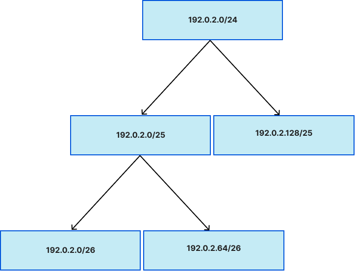
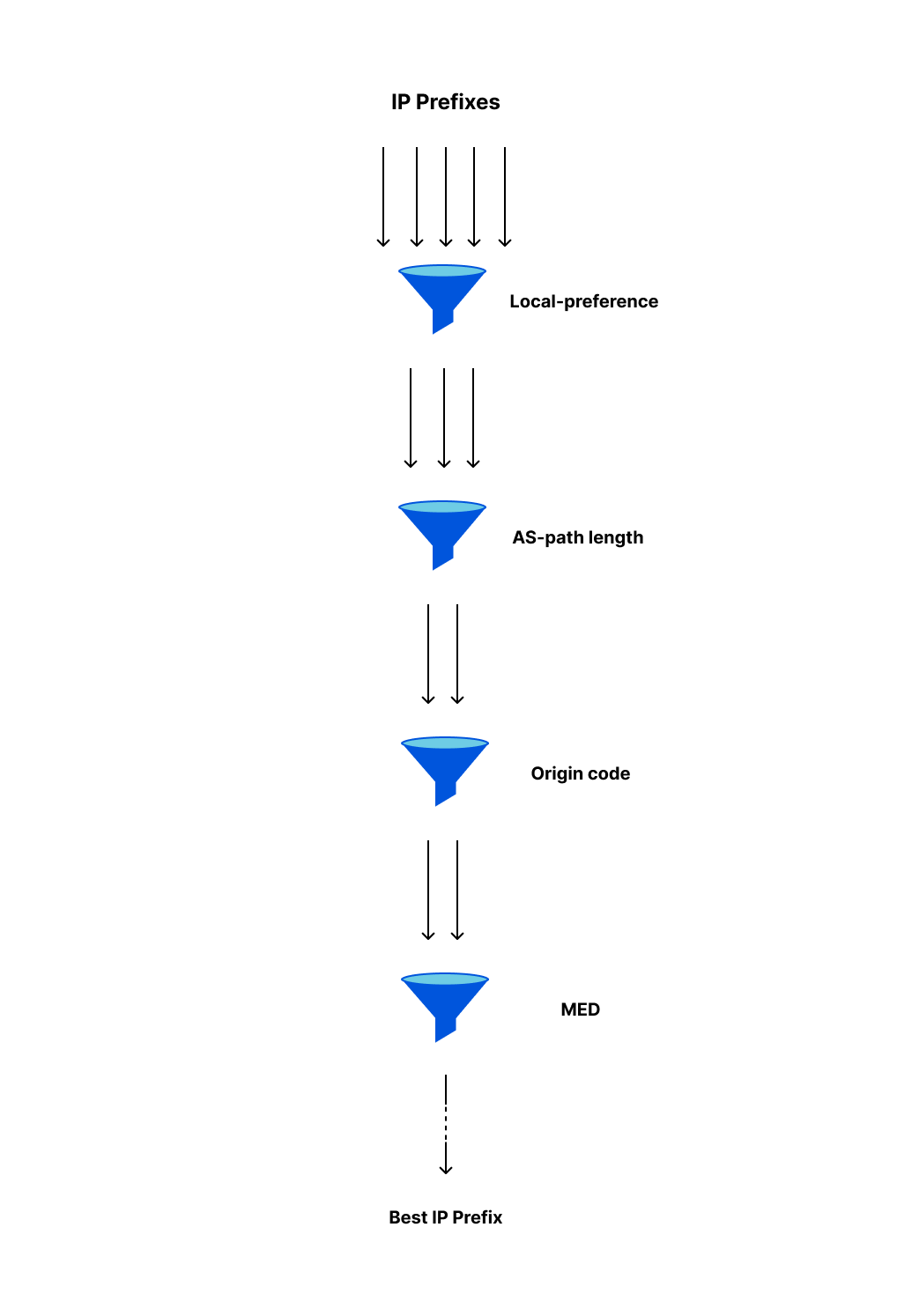
To understand the slowness that can often lead to BGP zombies, we need to talk about path hunting. Path hunting occurs when routers running BGP exhaustively search for the best path to a prefix as determined by Longest Prefix Matching (LPM) and BGP routing attributes like path length and local preference. This becomes relevant in our observations of exactly how routes become stuck, for how long they become stuck, and how visible they are on the Internet.
For example, path hunting happens when a more-specific BGP prefix is withdrawn from the global routing table, and networks need to fallback to a less-specific BGP advertisement. In this example, we use 2001:db8::/48 for the more-specific BGP announcement and 2001:db8::/32 for the less-specific prefix. When the /48 is withdrawn by the originating Autonomous System (AS), BGP routers have to recognize that route as missing and begin routing traffic to IPs such as 2001:db8::1 via the 2001:db8::/32 route, which still remains while the prefix 2001:db8::/48 is gone.
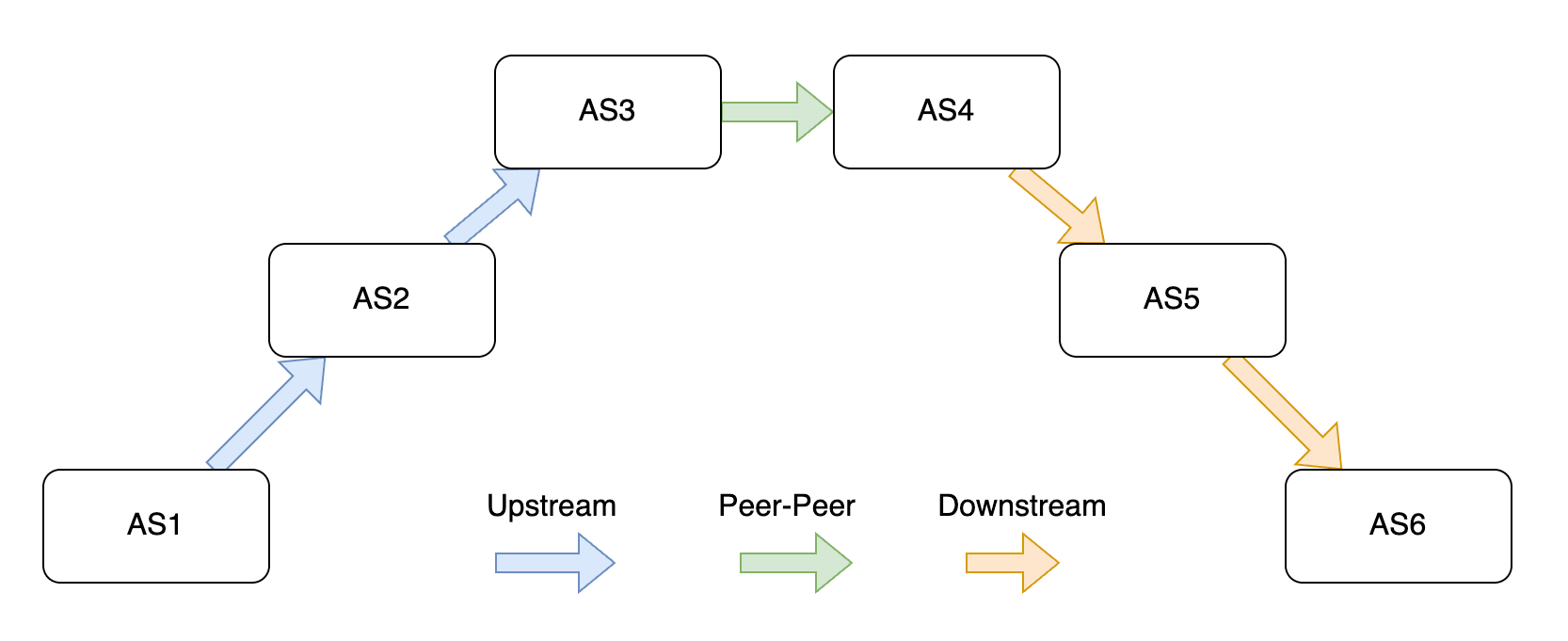
Let’s see what this could look like in action with a few diagrams.

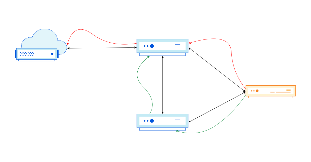
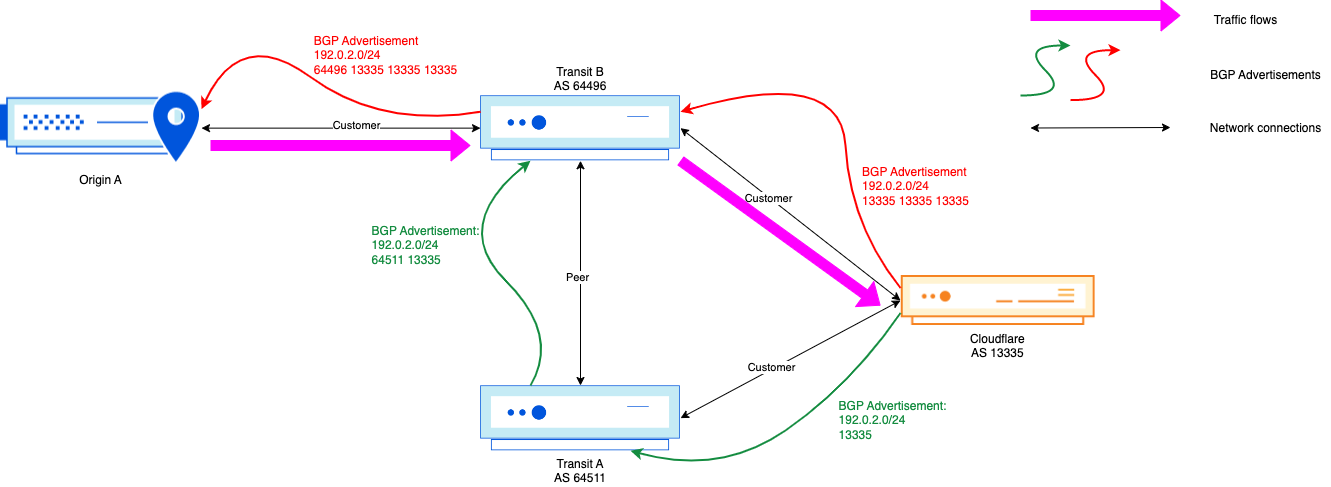
Diagram 1: Active 2001:db8::/48 route
In this initial state, 2001:db8::/48 is used actively for traffic forwarding, which all flows through AS13335 on the way to AS64511. In this case, AS64511 would be a BYOIP customer of Cloudflare. AS64511 also announces a backup route to another Internet Service Provider (ISP), AS64510, but this route is not active even in AS64510’s routing table for forwarding to 2001:db8::1 because 2001:db8::/48 is a longer prefix match when compared to 2001:db8::/32.
Things get more interesting when AS64510 signals for 2001:db8::/48 to be withdrawn by Cloudflare (AS13335), perhaps because a DDoS attack is over and the customer opts to use Cloudflare only when they are actively under attack.
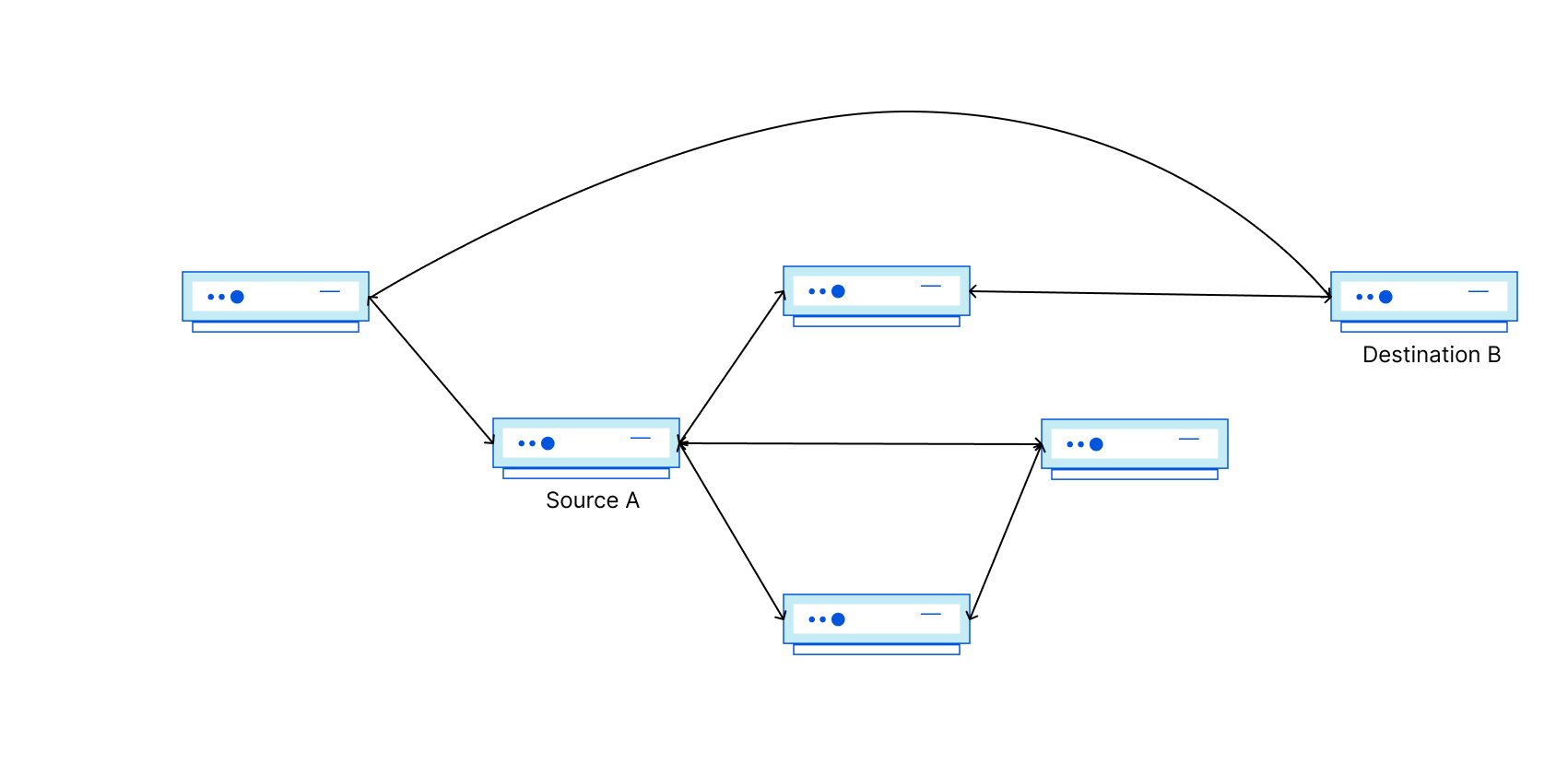
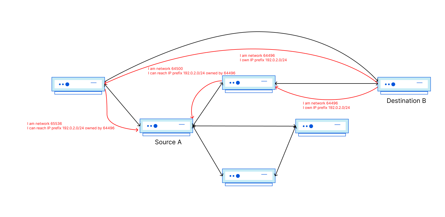
When the customer signals to Cloudflare (via BGP Control or API call) to withdraw the 2001:db8::/48 announcement, all BGP routers have to converge upon this update, which involves path hunting. AS13335 sends a BGP withdrawal message for 2001:db8::/48 to its directly-connected BGP neighbors. While the news of withdrawal may travel quickly from AS13335 to the other networks, news may travel more quickly to some of the neighbors than others. This means that until everyone has received and processed the withdrawal, networks may try routing through one another to reach the 2001:db8::/48 prefix – even after AS13335 has withdrawn it.

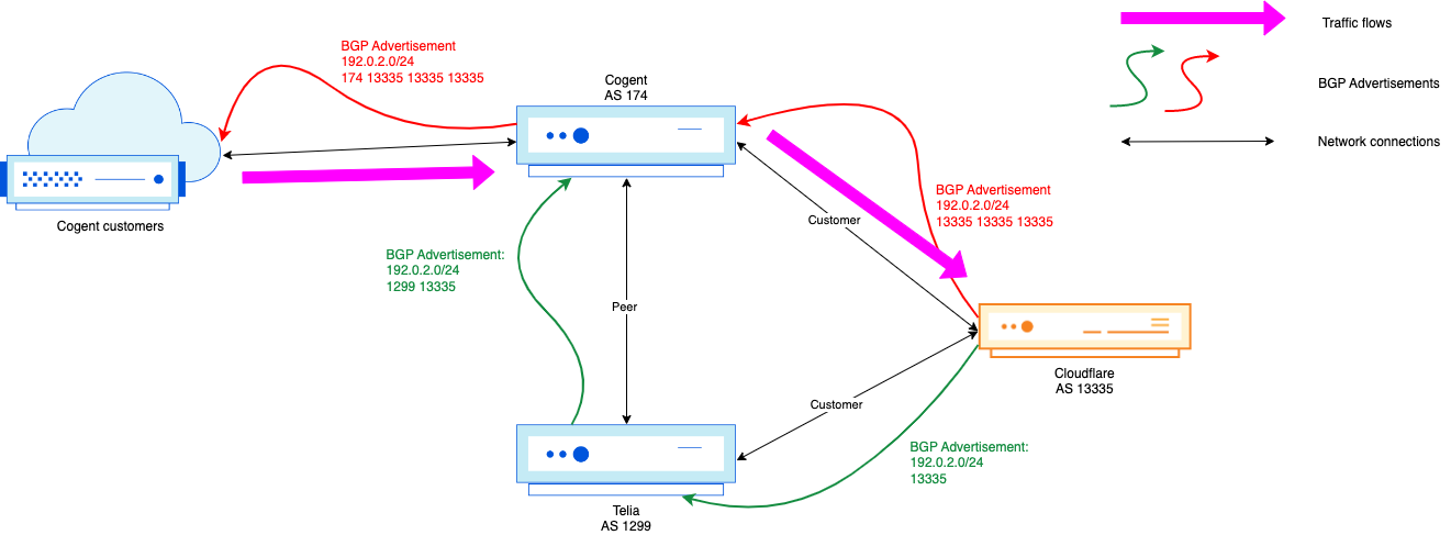
Diagram 2: 2001:db8::/48 route withdrawn via AS13335
Imagine AS64501 is a little slower than the rest – perhaps due to using older hardware, hardware being overloaded, a software bug, specific configuration settings, poor luck, or some other factor – and still has not processed the withdrawal of the /48. This in itself could be a BGP zombie, since the route is stuck for a small period. Our pings toward 2001:db8::1 are never able to actually reach AS64511, because AS13335 knows the /48 is meant to be withdrawn, but some routers carrying a full table have not yet converged upon that result.
The length of time spent path hunting is amplified by something called the Minimum Route Advertisement Interval (MRAI). The MRAI specifies the minimum amount of time between BGP advertisement messages from a BGP router, meaning it introduces a purposeful number of seconds of delay between each BGP advertisement update. RFC4271 recommends an MRAI value of 30-seconds for eBGP updates, and while this can cut down on the chattiness of BGP, or even potential oscillation of updates, it also makes path hunting take longer.
At the next cycle of path hunting, even AS64501, which was previously still pointing toward a nonexistent /48 route from AS13335, should find the /32 advertisement is all that is left toward 2001:db8::1. Once it has done so, the traffic flow will become the following:

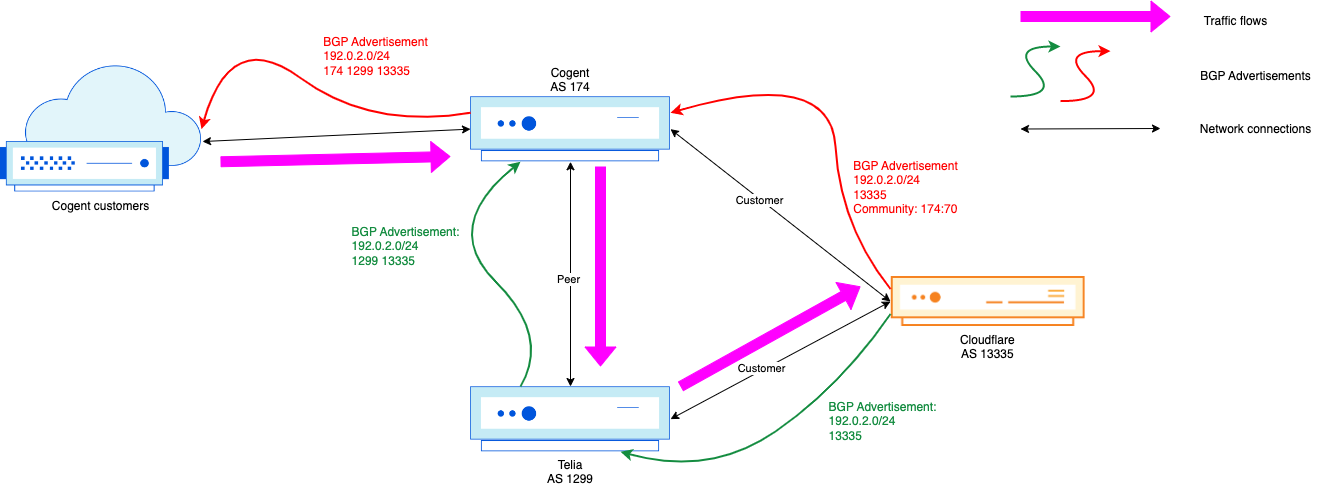
Diagram 3: Routing fallback to 2001:db8::/32 and 2001:db8::/48 is gone from DFZ
This would mean BGP path hunting is over, and the Internet has realized that the 2001:db8::/32 is the best route available toward 2001:db8::1, and that 2001:db8::/48 is really gone. While in this example we’ve purposely made path hunting only last two cycles, in reality it can be far more, especially with how highly connected AS13335 is to thousands of peer networks and Tier-1’s globally.
Now that we’ve discussed BGP path hunting and how it works, you can probably already see how a BGP zombie outbreak can begin and how routing tables can become stuck for a lengthy period of time. Excessive BGP path hunting for a previously-known more-specific prefix can be an early indicator that a zombie could follow.
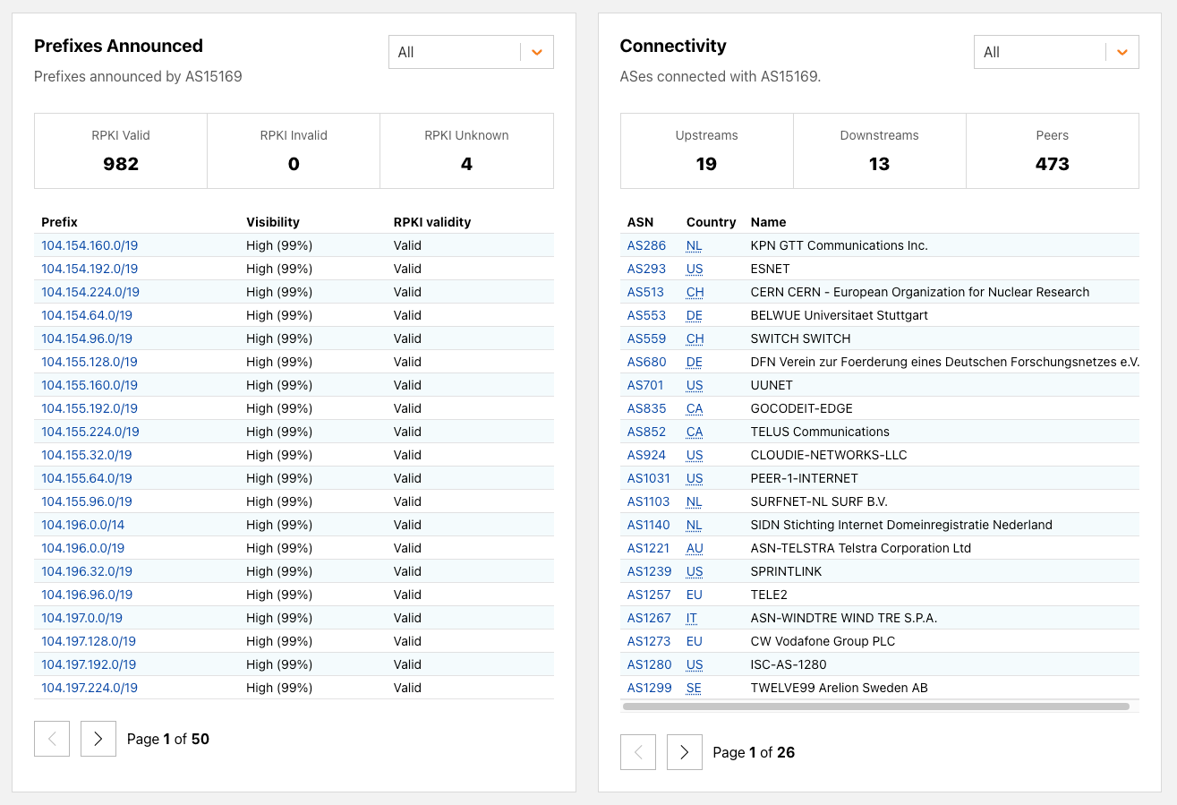
Zombies have captured our attention more recently as they were noticed by some of our customers leveraging Bring-Your-Own-IP (BYOIP) on-demand advertisement for Magic Transit. BYOIP may be configured in two modes: “always-on”, in which a prefix is continuously announced, or “on-demand”, where a prefix is announced only when a customer chooses to. For some on-demand customers, announcement and withdrawal cycles may be a more frequent occurrence, which can lead to an increase in BGP zombies.
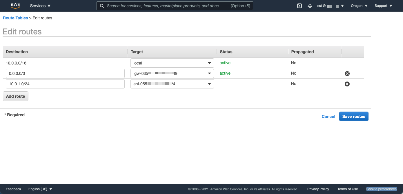
With that in mind and also knowing how path hunting works, let’s spawn our own zombie onto the Internet. To do so, we’ll take a spare block of IPv4 and IPv6 and announce them like so:

Once the routes are announced and stable, we’ll then proceed to withdraw the more specific routes advertised via Cloudflare globally. With a few quick clicks, we’ve successfully re-animated the dead.
Variant A: Ghoulish Gateways
One place zombies commonly occur is between upstream ISPs. When one router in a given ISP’s network is a little slower to update, routes can become stuck.
Take, for example, the following loop we observed between two of our upstream partners:
7. be2431.ccr31.sjc04.atlas.cogentco.com
8. tisparkle.sjc04.atlas.cogentco.com
9. 213.144.177.184
10. 213.144.177.184
11. 89.221.32.227
12. (waiting for reply)
13. be2749.rcr71.goa01.atlas.cogentco.com
14. be3219.ccr31.mrs02.atlas.cogentco.com
15. be2066.agr21.mrs02.atlas.cogentco.com
16. telecomitalia.mrs02.atlas.cogentco.com
17. 213.144.177.186
18. 89.221.32.227
Or this loop – observed on the same withdrawal test – between two different providers:
15. if-bundle-12-2.qcore2.pvu-paris.as6453.net
16. if-bundle-56-2.qcore1.fr0-frankfurt.as6453.net
17. if-bundle-15-2.qhar1.fr0-frankfurt.as6453.net
18. 195.219.223.11
19. 213.144.177.186
20. 195.22.196.137
21. 213.144.177.186
22. 195.22.196.137
Variant B: Undead LAN (Local Area Network)
Simultaneously, zombies can occur entirely within a given network. When a route is withdrawn from Cloudflare’s network, each device in our network must individually begin the process of withdrawing the route. While this is generally a smooth process, things can still become stuck.
Take, for instance, a situation where one router inside of our network has not yet fully processed the withdrawal. Connectivity partners will continue routing traffic towards that router (as they have not yet received the withdrawal) while no host remains behind the router which is capable of actually processing the traffic. The result is an internal-only looping path:
10. 192.0.2.112
11. 192.0.2.113
12. 192.0.2.112
13. 192.0.2.113
14. 192.0.2.112
15. 192.0.2.113
16. 192.0.2.112
17. 192.0.2.113
18. 192.0.2.112
19. 192.0.2.113
Unlike most fictionally-depicted hoards of the walking dead, our highly-visible zombie has a limited lifetime in most major networks – in this instance, only around around 6 minutes, after which most had re-converged around the less-specific as the best path. Sadly, this is on the shorter side – in some cases, we have seen long-lived zombies cause reachability issues for more than 10 minutes. It’s safe to say this is longer than most network operators would expect BGP convergence to take in a normal situation.
But, you may ask – is this the excessive path hunting we talked about earlier, or a BGP zombie? Really, it depends on the expectation and tolerance around how long BGP convergence should take to process the prefix withdrawal. In any case, even over 30 minutes after our withdrawal of our more-specific prefix, we are able to see zombie routes in the route-views public collectors easily:
~ % monocle search --start-ts 2025-10-28T12:40:13Z --end-ts 2025-10-28T13:00:13Z --prefix 198.18.0.0/24
A|1761656125.550447|206.82.105.116|54309|198.18.0.0/24|54309 13335 395747|IGP|206.82.104.31|0|0|54309:111|false|||route-views.ny
You might argue that six to eleven minutes (or more) is a reasonable time for worst-case BGP convergence in the Tier-1 network layer, though that itself seems like a stretch. Even setting that aside, our data shows that very real BGP zombies exist in the global routing table, and they will negatively impact traffic. Curiously, we observed the path hunting delay is worse on IPv4, with the longest observed IPv6 impact in major (Tier-1) networks being just over 4 minutes. One could speculate this is in part due to the much higher number of IPv4 prefixes in the Internet global routing table than the IPv6 global table, and how BGP speakers handle them separately.

Source: RIPEstat’s BGPlay
Part of the delay appears to originate from how interconnected AS13335 is; being heavily peered with a large portion of the Internet increases the likelihood of a route becoming stuck in a given location. Given that, perhaps a zombie would be shorter-lived if we operated in the opposite direction: announcing a less-specific persistently to 13335 and announcing more specifics via our local ISP during normal operation. Since the withdrawal will come from what is likely a less well-peered network, the time-to-convergence may be shorter:

Indeed, as predicted, we still get a stuck route, and it only lives for around 20 seconds in the Tier-1 network layer:
19. be12488.ccr42.ams03.atlas.cogentco.com
20. 38.88.214.142
21. be2020.ccr41.ams03.atlas.cogentco.com
22. 38.88.214.142
23. (waiting for reply)
24. 38.88.214.142
25. (waiting for reply)
26. 38.88.214.142
Unfortunately, that 20 seconds is still an impactful 20 seconds – while better, it’s not where we want to be. The exact length of time will depend on the native ISP networks one is connected with, and it could certainly ease into the minutes worth of stuck routing.
In both cases, the initial time-to-announce yielded no loss, nor was a zombie created, as both paths remained valid for the entirety of their initial lifetime. Zombies were only created when a more specific prefix was fully withdrawn. A newly-announced route is not subject to path hunting in the same way a withdrawn more-specific route is. As they say, good (new) news travels fast.
Our findings lead us to believe that the withdrawal of a more-specific prefix may lead to zombies running rampant for longer periods of time. Because of this, we are exploring some improvements that make the consequences of BGP zombie routing less impactful for our customers relying on our on-demand BGP functionality.
For the traffic that does reach Cloudflare with stuck routes, we will introduce some BGP traffic forwarding improvements internally that allow for a more graceful withdrawal of traffic, even if routes are erroneously pointing toward us. In many ways, this will closely resemble the BGP well-known no-export community’s functionality from our servers running BGP. This means even if we receive traffic from external parties due to stuck routing, we will still have the opportunity to deliver traffic to our far-end customers over a tunneled connection or via a Cloudflare Network Interconnect (CNI). We look forward to reporting back the positive impact after making this improvement for a more graceful draining of traffic by default.
For the traffic that does not reach Cloudflare’s edge, and instead loops between network providers, we need to use a different approach. Since we know more-specific to less-specific prefix routing fallback is more prone to BGP zombie outbreak, we are encouraging customers to instead use a multi-step draining process when they want traffic drained from the Cloudflare edge for an on-demand prefix without introducing route loops or blackhole events. The draining process when removing traffic for a BYOIP prefix from Cloudflare should look like this:
-
The customer is already announcing an example prefix from Cloudflare, ex. 198.18.0.0/24
-
The customer begins natively announcing the prefix 198.18.0.0/24 (i.e. the same-length as the prefix they are advertising via Cloudflare) from their network to the Internet Service Providers that they wish to fail over traffic to.
-
After a few minutes, the customer signals BGP withdrawal from Cloudflare for the 198.18.0.0/24 prefix.
The result is a clean cut over: impactful zombies are avoided because the same-length prefix (198.18.0.0/24) remains in the global routing table. Excessive path hunting is avoided because instead of routers needing to aggressively seek out a missing more-specific prefix match, they can fallback to the same-length announcement that persists in the routing table from the natively-originated path to the customer’s network.

Source: RIPEstat’s BGPlay
We are going to continue to refine our methods of measuring BGP zombies, so you can look forward to more insights in the future. There is also work from others in the community around zombie measurement that is interesting and producing useful data. In terms of combatting the software bugs around BGP zombie creation, routing vendors should implement RFC9687, the BGP SendHoldTimer. The general idea is that a local router can detect via the SendHoldTimer if the far-end router stops processing BGP messages unexpectedly, which lowers the possibility of zombies becoming stuck for long periods of time.
In addition, it’s worth keeping in mind our observations made in this post about more-specific prefix announcements and excessive path hunting. If as a network operator you rely on more-specific BGP prefix announcements for failover, or for traffic engineering, you need to be aware that routes could become stuck for a longer period of time before full BGP convergence occurs.
If you’re interested in problems like BGP zombies, consider coming to work at Cloudflare or applying for an internship. Together we can help build a better Internet!