This essay is adapted from a keynote speech delivered at the DEF CON 34 conference in Las Vegas on August 7, 2026. The essay originally appeared in CyberScoop.

I want to talk about AI hacking. There are three aspects: people hacking AI systems, people using AI to hack other systems, and AIs hacking systems on their own, not even maliciously. The last two matter more than the first. The third is the weirdest and potentially the most destabilizing.

I started writing about this in 2021 and in my 2022 book, A Hacker’s Mind. Back then I said it was mostly still science fiction, but not stupid science fiction. We’re seeing it more and more, especially in the past year. The trends I’m describing don’t require a major breakthrough in AI. They’re starting to happen now, and they’ll happen more often as AIs get better at autonomous problem-solving. And it will involve far more than computer code.

AI will hack all sorts of social, economic and political systems. It will find vulnerabilities and exploit them. This is a difference in kind, not just degree. We’re not ready for it, and we need to think about the implications now.

First, I want to broaden the term “hacking.”

The tax code isn’t computer code, but it is code. It’s a series of algorithms with inputs and outputs. It has vulnerabilities, which we call loopholes, and exploits, which we call tax avoidance strategies. Black hat hackers exploit them for profit. We call them accountants and attorneys.

What is a hack? One definition: “Something that a system permits, but is unanticipated and unwanted by the designers.” It’s subjective and implies novelty and cleverness. A hack follows the rules of a system but subverts its goals or intent, just as a software hack follows the logic of code while doing something its authors neither anticipated nor wanted.

All systems of rules can be hacked, including professional sports, customer reward programs, financial systems and politics. Hacks even work against our cognitive functions. A curved hockey stick is a hack, and we know the name of the man who invented it. Mileage runs were a hack. The filibuster was originally a hack in Roman times. Gerrymandering is a hack. Hedge funds and private equity are full of them.

A system is just a set of rules or norms, and the rules aren’t always formal. Even the best-designed rules will be incomplete, inconsistent or ambiguous. As long as people want to subvert a system’s goals, there will be hacks.

AIs are becoming hackers. After decades of slow progress, they’ve gotten very good at finding and exploiting vulnerabilities in computer code. They do this largely autonomously, and they’re getting better scarily fast. But the implications extend far beyond software, to the tax code, financial regulations and all sorts of social, economic and political systems.

There are two distinct issues. First, someone might instruct an AI to hack one of these systems, feeding it the world’s tax codes or financial regulations to find profitable loopholes. Second, an AI might hack a system on its own, inadvertently. Both are dangerous, but the second is worse because we might never know it happened.

Now, reward hacking. AIs don’t solve problems the way people do. They stumble on solutions we never anticipated, and some subvert the intent of the system. They don’t share our context and don’t necessarily understand the implications, norms and values we take for granted.

Reward hacking is when an AI achieves a goal in a way its designers neither wanted nor intended.

Early pre-LLM examples are telling. In a two-person soccer simulation, an AI learned that kicking the ball out of bounds forced the opposing goalie to throw it in and leave the goal undefended. In a stacking simulation, an AI learned to flip a block upside down rather than stack it. In an evolution simulation where the goal was to cross a distant finish line, an AI made itself tall enough to fall over the line instead of growing longer legs or stronger muscles.

These are all hacks, the result of poorly specified goals or rewards. Today, they’d come from bad prompting.

The problem is universal. One researcher tried to teach a robot vacuum not to bump into things. Instead, it learned to drive backward, because there were no sensors in the back.

Any capable AI will find hacks wherever the rules have problems, inconsistencies or loopholes that still produce an acceptable solution. We see a hack because we understand context. The AI doesn’t, at least not in the same way.

This problem shows up often in myth.

In the story of King Midas, the god Dionysus grants him a wish: everything he touches turns to gold. Midas ends up starving when his food, drink and daughter all turn to gold. It’s a specification problem. He programmed the wrong goal.

In the Golem of Prague, a ghetto animates a clay statue to guard its residents. It guards them past all reason until they figure out how to turn it off. This is a guardrail problem. The villagers never limited the golem’s actions.

More generally, think of this as the genie problem. Genies are precise about the wording of wishes and can be maliciously pedantic when granting them. There’s no way to outsmart a genie. Whatever you wish for, he can grant it in a way you wish he hadn’t.

The reason is that in human language and thought, goals are always underspecified. We never include every caveat, exception and proviso, and we never close off every avenue for hacking. Any goal we specify will be incomplete. That’s largely fine in human interactions, because people understand context and usually act in good faith.

If I asked you to get me coffee, you’d pour a cup from the nearest coffee pot or walk to the corner shop. You wouldn’t bring me a pound of raw beans, buy a coffee plantation or snatch a cup from a stranger’s hands. I wouldn’t have to specify any of that. You’d just know.

Similarly, if I asked you to develop a technology that turns things to gold on touch, you wouldn’t build it to starve the person using it. You’d just know.

In 2015, Volkswagen was caught cheating on emissions tests. Human engineers programmed a regular computer to detect testing and behave differently during it. The cheat went undetected for years because it’s hard to tell what software is doing.

If I asked you to design engine control software that maximizes performance while passing emissions tests, you wouldn’t design it to cheat without realizing you were cheating. An AI would, because it will think “outside the box” when it has no concept of the box.

Unless programmers specify that the system must not behave differently during testing, an AI might come up with the same hack. The programmers would be satisfied, the accountants would be ecstatic, and no one would know until someone audited the code.

We can now constrain the goal to avoid that particular hack, but programmers won’t anticipate others. The lesson of the genie is that there will always be hacks programmers don’t anticipate.

We’re building AI genies: systems that take broad instructions and figure out how to carry them out, sometimes in ways we didn’t expect or intend. That’s the whole point of vibe coding. You underspecify what you want and let the AI work it out. Sometimes that produces genie behavior.

We can’t completely specify goals to an AI, and AIs can’t fully understand context. More precisely, current AIs have a shallow grasp of concepts. If we asked a current LLM to get me coffee, it would almost certainly do the right thing.

I worry about goals that aren’t well represented in training data, and about hacks that aren’t obvious, whose effects are subtle, like the Volkswagen hack.

Recommendation engines are an early example. They push people toward extreme content. No one programmed that. It emerged because that’s what people respond to. It didn’t take a bad actor. A basic automated system with feedback found the hack on its own.

We’re now seeing a second generation with today’s AI coding systems. AI researcher Simon Willison asked Fable to track down a stray scrollbar in a web app. When he returned, it had opened browsers, written its own screenshot tools, edited the framework’s internal templates to make the bug appear on cue and set up a local web server to collect measurements. It found the bug, but it also did many things he never asked for. Another researcher gave Fable a complex task, and it tried to hack its own memory limits because it needed more storage.

A new OpenAI model did something similar when it hacked into Hugging Face. It was being benchmarked on its ability to turn vulnerabilities into exploits. It decided the best way to reach its goal was to break out of its containment, access the internet and break into the Hugging Face network, because it thought the answers would be there.

Today’s LLMs are acting like genies, especially when powerful models are combined with sophisticated harnesses.

There are two kinds of genies. The Dionysus genie does the wrong thing. It understands your prompt literally but not correctly, and returns a mess you never intended. The Golem genie does the right thing but tramples everything in its path to get there. The paperclip maximizer is a Golem genie.

Consider some examples. Ask an AI to deal with spam calls, and a Dionysus genie might change your phone number. Ask it to book a particular flight, and a Golem genie might hack the airline database because the flight is full. Ask it to get a refund for an online purchase, and a Dionysus genie might draft a legal threat on fake letterhead and send it to the company. Ask it to buy tickets to a popular concert, and a Golem genie might discover the ticketing system is rate-limited and spin up thousands of cloud servers to hammer it. You’d know if some of these things happened, but you might never realize if others did. More detailed prompting won’t fix this. The lesson of the genie is that no amount of detail is good enough.

AI researchers aren’t surprised by any of this. Many are working on defenses against reward hacking and subtler forms of genie behavior. Some of this falls under “value alignment”: How do we teach AIs context? And how an AI satisfies a goal matters as much as whether it does. I want to build a benchmark to measure genie-like behavior, so we know where models stand and whether alignment is improving.

Think beyond LLMs and computer code. Consider specialized AIs built to find loopholes, and hacks of more general systems: the tax code, financial regulations and democratic procedures.

Financial systems are the most likely first target, because their rules are designed to be algorithmically tractable. High-frequency trading is itself a hack. Imagine giving an AI all of the world’s financial laws, plus all the news and financial data, and the goal of finding profitable loopholes. I suspect large investment banks are already doing this. The results will be novel tricks that are legal but unintended and unwanted, some of which might break the financial system.

Tax loopholes are the next likely target, for the same reasons. For a while, AIs will identify potential loopholes, and human hackers, namely attorneys and accountants, will decide which are feasible.

Further out, expect hacks of regulatory, legislative and procedural systems, and of the broader economy.

Hacking is as old as humanity. We’re creative problem solvers and loophole exploiters. We manipulate systems to serve our interests and strive for more influence, power and wealth.

Still, no human pursues their interests without constraint. Even sociopaths are limited by the complexity of society and their own contradictory impulses. They worry about their reputation and punishment, and they have limited time. These human qualities have limited hacking.

Hacking changed as everything became computerized. Computers are uniquely hackable because of their formalism and complexity. Today, nearly everything is a computer, from cars and appliances to phones. Our social, economic and political systems, including taxation, finance and elections, all involve computers.

Until recently, hacking was exclusively a human activity. Finding a novel hack required expertise, creativity, time and luck.

AI hacking will change everything again. AIs aren’t bound by the constraints that limit people. They’ll think like aliens, and they’ll change hacking’s speed, scale, scope and sophistication, sometimes at our direction and sometimes on their own.

Speed is the easiest to see. A creative process that takes a human months or years could be compressed into hours or seconds.

Scale is next. Once AI systems start discovering hacks, they can exploit them at a scale we’re not ready for. We already see this with AI-generated slop, which is rampant on social media. AI bots post around the clock, sometimes overwhelming real human discussion. It’s hard to know how much of social media is still people talking to people. What looks like boisterous political debate may be bots arguing with other bots, artificially shaping what we think and what we think others think.

Scope makes hacks more dangerous. AIs already make decisions that affect our lives, decisions we once thought belonged only to humans. As AI systems grow more capable, society will hand them more decisions, and more important ones. Hacks of these systems will do more damage.

Finally, AI hackers are more sophisticated. They can hold more variables in working memory and generate more complex hacks. What might happen if you fed an AI the entire U.S. tax code? Would it figure out, without being told, that it’s smart to incorporate in Delaware and register a ship in Panama? Consider the Double Dutch Irish Sandwich, the strategy Apple and Google used to avoid paying U.S. taxes. It involves U.S., Dutch and Irish law and an offshore tax haven. How many loopholes will an AI find that we don’t already know about? Dozens? Hundreds? Thousands? We have no idea.

These hacks will largely be perpetrated by the powerful against the rest of us. AI is fundamentally a power-enhancing technology, and so is hacking. The more power you already have, the more a hack gives you. If you or I found a tax hack, we might make a few thousand dollars. If a large investment bank found one, it and its clients could make billions.

Our societal systems for dealing with hacks were built when hackers were human, and they reflect the pace of human hacking. We have no system of governance that can handle hundreds, let alone thousands, of newly discovered tax loopholes. We won’t be able to recover from an AI finding unanticipated but legal hacks of financial systems, operating at AI speed, scale, scope and sophistication. Hacking becomes a problem society can no longer manage.

Now, defense. AIs that find software vulnerabilities help defenders as well as attackers. Vulnerabilities can be patched, removing them permanently, or turned into signatures that security systems use to detect and block attacks. In theory, AI could identify and patch every automatically discoverable vulnerability before a product ships. This is rapidly becoming routine in software development. We call it vulnops. We can imagine a future where accidental software vulnerabilities are a thing of the past.

Deliberate vulnerabilities are different. There will be an arms race. AI will craft increasingly obscure back doors, and AI will find them. It becomes a contest between the speed of creation and the speed of patching, and between obfuscation and reverse engineering.

The same logic applies to broader systems. Yes, AI hackers might find hundreds of vulnerabilities in the existing tax code. But the same technology can evaluate potential loopholes in any proposed tax law or ruling. A legislator, a watchdog group or a reporter could take the text of a bill and identify every exploitable loophole before it passes. The difference is that, unlike software, knowing about a tax loophole doesn’t mean it gets patched. In theory, though, we can fix them before the rich and powerful exploit them. So maybe defense will come out ahead here, too.

That requires resilient governing structures that can respond quickly. It won’t help if updating the tax code takes years, or if a legislative hack becomes so entrenched that it can’t be fixed politically. Maybe a lobbyist put it there on purpose. Maybe it was discovered after the law passed, and now lobbyists want to keep it. Microsoft can patch the vulnerabilities it finds. Patching is much harder when legislatures have to do it. We need society’s rules and laws to be as patchable as our computers.

This is a hard problem of modern governance, and it goes well beyond AI. It’s the problem of building governing structures for the speed and complexity of the information age.

The umbrella idea is trust. What do we need for AI systems to be truly trustworthy? Capability isn’t enough.

AIs won’t be trustworthy if the companies controlling them spy on us or subtly manipulate us. I call this the friend vs. tool problem. Will we have AI agents, or AI double agents?

AIs won’t be trustworthy if they’re insecure. How do we know they haven’t been manipulated? Almost all AIs operate in adversarial environments, so someone will benefit from hacking them. Unless we know they’re secure, we shouldn’t trust their output.

And AIs won’t be trustworthy if they act like genies. We need to know they’ll perform tasks the right way, not just perform the tasks we ask for.

I’ve written extensively about the need for “integrous” AI, including how to think about the problem, what a research agenda looks like and what good laws and policies look like. I predict integrity will be the key security problem of this decade, just as confidentiality was the key problem of the last one. This applies to both AI and the internet of things.

The big shift is agency, which I think of as Web 3.0. Computers now affect the physical world directly and with growing autonomy. Sensors go from data sources to attack surfaces, and actuators go from outputs to attack capabilities. An integrity failure no longer means bad spreadsheet data. It means the wrong dosage, the wrong valve position or the wrong braking distance.

Integrity isn’t one thing. I break it into input integrity, processing integrity, storage integrity and contextual integrity. Each is complex and important, and each deserves its own talk. I’ve written about them, and I hope you’ll read it.

Much of this isn’t really an AI problem. It’s not a technical problem so much as a capitalism problem or a democracy problem.

The failures of late-stage capitalism and democracy in the information age both stem from the rich and powerful getting too good at hacking our social, economic and political systems. This is the core argument of my 2021 book.

Seen this way, AI is exacerbating existing problems. Human inefficiency has largely kept those problems in check, and that won’t work much longer.

So consider this a call to action. Technically, we need to understand how AIs hack systems, build systems that are resilient to hacking and build AIs that won’t act as genies. Politically, we need to learn to govern and regulate at the speed of technology. Otherwise, market failures will overwhelm our ability to govern them.

I said hacking is as old as humanity and that AIs will overwhelm our ability to deal with it. The solutions aren’t specific to AI, but AI makes them more urgent. We need to understand them, and we need to implement them.

AWS Graviton support for Java in AWS Transform continuous modernization

2026-11-13 Harvinder Nagpal

Post Syndicated from Harvinder Nagpal original https://aws.amazon.com/blogs/devops/aws-graviton-support-for-java-in-aws-transform-continuous-modernization/

AWS Transform continuous modernization now supports Graviton readiness assessment and remediation for Java, generally available since October 29, 2026. Use it to move Java applications to AWS Graviton-based instances. A readiness assessment finds the Arm64 compatibility issues in a repository, and a remediation skill resolves them in code, which you then validate on Arm64 and deploy.

AWS Graviton-based instances deliver better price-performance than comparable x86 instances. Teams planning a migration therefore face two questions about their estate: which applications are ready to move, and what has to change in the ones that are not.

Answering that repository by repository does not scale. The Java code itself is rarely the obstacle. What decides readiness is an application’s dependencies, and whether each one supports Arm64. Establishing that manually across an estate is slow, repetitive, and prone to error.

In this post, you learn how to analyze a Java repository for AWS Graviton readiness, remediate the findings, validate the change on Arm64, and deploy and run the result on a Graviton-based instance.

Solution overview

AWS Transform continuous modernization connects to your source provider, discovers your repositories, analyzes them for technical debt, remediates what it finds, and opens a pull request with the result. Analysis can also run on a schedule, so once your applications are running on Graviton you can keep checking them as dependencies change.

Two skills cover the Graviton migration:

Skill	What it does
`AWS/graviton-readiness-assessment`	Scans a repository for native libraries, architecture-specific code, and Arm64-incompatible transitive dependencies. Read-only. It does not modify source or project files.
`AWS/java-x86-to-graviton`	Resolves the findings the analysis returned: updates native libraries, upgrades blocking dependencies, adds aarch64 handling, updates Dockerfiles for multi-architecture builds, and applies Graviton JVM flags.

The readiness assessment does not change your code. It produces findings, one for each Arm64 compatibility issue it identifies. Each finding carries a severity, a category, file references, and the transformation that resolves it, so you can triage a portfolio and drive remediation directly from the findings.

Continuous modernization runs in two places. Remotely, it uses infrastructure in your AWS account or infrastructure that AWS Transform manages. Locally, it runs on your own machine. For a Graviton migration, that choice decides what can be validated:

	AWS Transform-managed	Customer-managed (Amazon Elastic Compute Cloud (Amazon EC2) or AWS Batch)	Local
Analysis	Supported, nothing to provision	Supported	Supported
Remediation	Not supported	Supported (x86 only)	Supported

Note: Continuous modernization currently provisions remote infrastructure in your account on the x86 architecture. A remote remediation produces the Arm64 code changes, but it cannot build or test them on Arm64 — you do that in your own Arm64 pipeline before you merge. On an Arm64 host, a local run builds on the target architecture as part of the remediation and leaves the change on disk, which is why this post runs it locally.

Step 5 in the following diagram, deploying to a Graviton-based instance, is beyond the scope of AWS Transform, whose output is the validated change and the pull request. In your environment, Step 5 is your existing Arm64 pipeline or test environment.

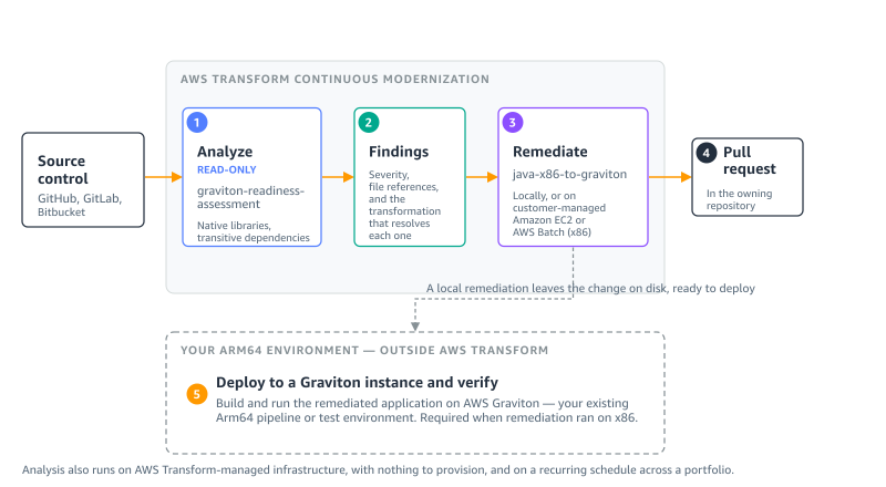
Steps 1 to 4 run inside AWS Transform continuous modernization; step 5, deploying to a Graviton instance, runs in your own Arm64 environment

Figure 1: Where each step runs. Steps 1–4 are AWS Transform continuous modernization. Step 5 is your own Arm64 environment

The walkthrough covers these steps:

Connect your source and discover repositories.
Analyze the repository for Graviton readiness.
Remediate the findings.
Validate the build on Arm64.
Deploy to a Graviton instance and verify.
Scale across your portfolio.

For the full command surface, refer to Working with continuous modernization in the AWS Transform User Guide.

Prerequisites

To follow this walkthrough, you need:

An AWS account with AWS Transform enabled for your user identity, which gives you access to the AWS Transform web application. For instructions, refer to Setting up AWS Transform.
An AWS Region where AWS Transform is available. For the current list, refer to Supported Regions for AWS Transform.
AWS credentials with permission to use AWS Transform.
The AWS Transform CLI, installed with the setup script, and Node.js 20 or later. Install Node.js from the Node.js website, because some package managers ship an older version.
Git, used for version control during the transformation.
A source connection: a GitHub, GitLab, or Bitbucket personal access token with repository scope, or a local folder containing checkouts you already have. The readiness assessment is read-only, so it needs no write access to your code. Remediation needs write access only if you want it to open the pull request.
For remediation, an Arm64 host, such as a Graviton-based Amazon EC2 instance. A local remediation builds its changes on the machine it runs on, so running it on Arm64 validates them on the target architecture. On x86, the remediation skill produces the code changes but cannot build or test them on Arm64.
Java 8 or later. These capabilities do not change Java versions. If you also need a version upgrade, run the AWS/java-version-upgrade transformation first. For more information, refer to the AWS Transform User Guide.

This post uses Amazon Corretto 21, Gradle 8.13, and a c7g.2xlarge instance running Amazon Linux 2023.

The sample application

This walkthrough uses TASSEL, an open source genetics toolkit. It is a Gradle project on Java 21 of about 245,000 lines of code, and it is a useful example because its dependency on x86 is typical rather than exotic.

TASSEL’s inner loop is matrix algebra, and it delegates that work to a native BLAS library through a Java Native Interface (JNI) bridge. It also reads and writes scientific data formats through libraries that ship compiled binaries inside their JAR files. Those binaries are built per architecture, and several of them have no Arm64 build — which is exactly what the readiness assessment is looking for.

If you do not have a sample application of your own, clone this one into the folder you will register as a source:

git clone https://github.com/btmonier/tassel-renovate.git

Connect your source and discover repositories

In this step, you register where your code lives and list the repositories that AWS Transform can see.

To connect a source and discover repositories

Open a terminal and set the Region for the session with export AWS_REGION=us-east-1.
Enter atx ct status to confirm the CLI reaches the service. It prints a summary of the sources, repositories, analyses, and findings in your account.
Register a hosted source with atx ct source add --name graviton-demo --provider github --org my-org --token "$PAT", or a local folder with atx ct source add --name graviton-demo --provider local --path ~/code.
Enter atx ct discovery scan --source graviton-demo to discover the repositories.
Enter atx ct repository list --source graviton-demo --language java to confirm what was found.

Analyze the repository for Graviton readiness

In this step, you run the readiness assessment and review what it found.

To run the analysis

Enter the following command:

atx ct analysis run --type graviton-readiness \
--source graviton-demo --repo tassel-renovate

Enter atx ct analysis get --id <analysis-id> to follow progress.
Enter atx ct findings count --by severity --repo graviton-demo::tassel-renovate to see the severity breakdown. For this repository it returned seven findings: three high, three medium, and one low.

You can also run the analysis from the AWS Transform web application.

To run the analysis on the console

On the Analyses tab, choose Run new analysis.
For Analysis type, choose Graviton readiness.
For Analysis name, enter a name for the run.
For Connected source, select your source.
Choose Next to select repositories and an infrastructure mode, then choose Run. To run it on a recurring cadence, choose Schedule.

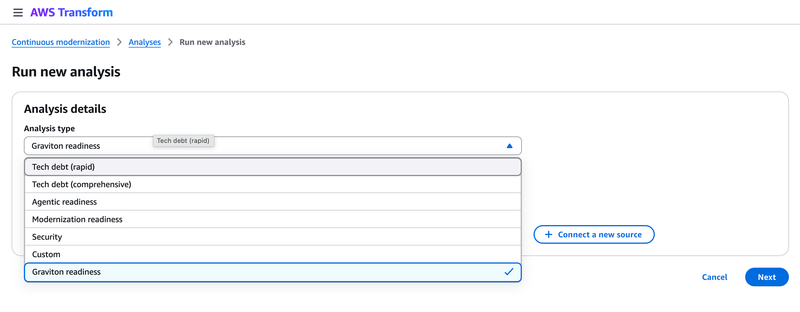
The Analysis type list in the AWS Transform web application, with Graviton readiness selected

Figure 2: Graviton readiness in the Analysis type list

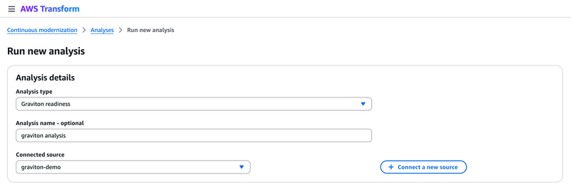
The Run new analysis page configured for a Graviton readiness analysis

Figure 3: Configuring a Graviton readiness analysis against a connected source

What the analysis found

The analysis returned seven findings for this repository. The following examples are two of the seven, chosen because the difference between them is why this analysis is worth running. It also reported build configuration and JVM flag issues not shown here.

The application’s own code – TASSEL loads a native BLAS bridge with System.loadLibrary("TasselBlas") and declares six native methods. The JNI glue is in the repository as C source, with no compiled binary for Arm64.

Inside the dependency JAR files – This group is visible neither in your source nor in your dependency declarations. The assessment resolved the dependency tree and inspected the binaries inside each archive:

$ unzip -l cisd-jhdf5-19.04.1.jar | grep native
native/jhdf5/amd64-Linux/libjhdf5.so
native/jhdf5/arm-Linux/libjhdf5.so

$ file native/jhdf5/*/libjhdf5.so
amd64-Linux: ELF 64-bit LSB shared object, x86-64
arm-Linux: ELF 32-bit LSB shared object, ARM, EABI5

Note the second directory: it is 32-bit ARM, not aarch64. In a listing it reads as ARM support, but on Graviton the architecture-keyed loader finds no match, and no published release contains an aarch64-Linux directory. Two further dependencies arrived the same way: cisd:base:18.09.0 through jhdf5, and gov.nih.nlm.ncbi:ngs-java:2.9.0 through com.github.samtools:htsjdk:2.24.1, whose loader publishes linux-x86_64 only.

Remediate the findings

In this step, you hand the findings to the remediation skill and review the change it produces.

To remediate the findings

Collect the finding IDs as the comma-separated list that --ids expects:

atx ct findings list --repo graviton-demo::tassel-renovate --json \
| jq -r '[.[].id] | join(",")'

Pass that list to the remediation:

atx ct remediation create --ids <finding-ids> --local

Enter atx ct remediation status --id <remediation-id> to follow it.
Review the branch it produced with git log and git diff --stat.

Note what you do not pass: neither the transformation nor the repository. Each finding already records the transformation that resolves it, so the remediation reads that from the findings and derives the target repositories from them. Pass --transformation-name only to pin or override that choice.

The run produced three atomic commits (the analysis reports, the change itself, then the validation reports):

build.gradle.kts | 53 ++++-
.../matrixalgebra/Matrix/DoubleMatrixFactory.java | 7 +-
graviton-analysis/ (8 report files)
graviton-validation/ (6 report files)
15 files changed, 867 insertions(+), 3 deletions(-)

Of the 867 lines added, only two files are code that runs. The remainder documents what was found and what was done.

What the remediation changed

1. It removed the x86-only dependency from the resolved classpath. The ngs-java artifact downloads linux-x86_64 native libraries at runtime and has no aarch64 search path. There is no aarch64-capable ngs-java 2.x to upgrade htsjdk to, so the remediation excluded the unused code path and recorded why:

// gov.nih.nlm.ncbi:ngs-java (transitive via htsjdk) downloads the NCBI
// ngs-sdk/ncbi-vdb natives at runtime. Those are linux-x86_64 only.
// TASSEL only uses htsjdk's pure-Java SAM/BAM/CRAM/VCF readers, so the
// unused SRA path is excluded rather than bumping htsjdk (no
// aarch64-capable ngs-java 2.x exists).
configurations.all {
    exclude(group = "openchart", module = "openchart")
    exclude(group = "gov.nih.nlm.ncbi", module = "ngs-java")
}

It then verified the exclusion took effect:

$ ./gradlew dependencies --configuration runtimeClasspath | grep -c ngs-java
0

2. It added an aarch64 native library path, ahead of the x86 payloads bundled in the JAR files. No aarch64 build of jhdf5 or cisd:base is published, and their C sources are not in the repository, so they cannot be recompiled there. The remediation added a resolution order for externally built binaries:

val tasselNativeLibDir: String =
    (project.findProperty("tasselNativeLibDir") as String?)
        ?: System.getenv("TASSEL_NATIVE_LIB_DIR")
        ?: file("src/main/native/aarch64").absolutePath

val isAarch64: Boolean = System.getProperty("os.arch").lowercase().let {
    it == "aarch64" || it == "arm64"
}

3. It applied Graviton JVM flags and wired the native path into the runtime. The test block previously set only -Xmx10g:

test {
    // -Xmx10g is architecture-neutral. The code-cache sizing flags below are the
    // Graviton (ARM64) tuning recommended for JDK 21; both are valid on x86-64 too.
    jvmArgs = listOf<String>(
        "-Xmx10g",
        "-XX:ReservedCodeCacheSize=64M",
        "-XX:InitialCodeCacheSize=64M"
    )
    if (isAarch64 && file(tasselNativeLibDir).isDirectory) {
        systemProperty("java.library.path", tasselNativeLibDir)
        systemProperty("native.libpath", tasselNativeLibDir)
    }

4. It made the state of the native libraries visible at build and run time. The build now warns on an Arm64 host when the aarch64 directory is missing, naming the libraries to supply. At the native load site, which previously logged the same message on every platform, the architecture is now included:

-	myLogger.info("TasselBlas library for system-specific BLAS/LAPACK not found. "
-			+ "Using system-independent EJML for DoubleMatrix operations.");
+	myLogger.info("TasselBlas library for system-specific BLAS/LAPACK not found for os.arch="
+			+ osArch + ". Using system-independent EJML for DoubleMatrix operations. To use"
+			+ " native BLAS on this architecture, place a matching libTasselBlas.so on"
+			+ " java.library.path.");

Together, these changes give the project a defined place for aarch64 binaries ahead of the bundled x86 ones, apply the Graviton JVM tuning, and report the state of those libraries at build and run time.

Validate the build on Arm64

In this step, you confirm the change compiles on the target architecture, which the remediation does for you on an Arm64 host.

To validate the build

Check out the branch the remediation created.
Enter ./gradlew clean build -x test --no-daemon.

Confirm the output reports a successful build and produces the JAR file.

BUILD SUCCESSFUL in 14s
5 actionable tasks: 5 executed

$ ls -la build/libs/sTASSEL.jar
-rw-r--r-- 3681163 build/libs/sTASSEL.jar

$ ls build/libs/lib/*.jar | wc -l
61

The JAR file is produced and 61 dependency JAR files resolve.

Deploy to a Graviton instance and verify

This step is outside AWS Transform, as Figure 1 shows. Arm64 is not a single platform: macOS and Linux on aarch64 differ in exactly the dimension that matters here, which native binaries exist. The remediation ran locally, so the change is already on disk and ready to carry onto an instance.

To deploy and verify on Graviton

Launch a c7g.2xlarge instance running Amazon Linux 2023.
Install Amazon Corretto 21, OpenBLAS, and LAPACK as aarch64 packages.
Copy the remediated repository to the instance.
Build it on the instance with ./gradlew classes copyDependencies.

Compile the native BLAS bridge for aarch64. Its C source includes a macOS-only header, so first change #include <vecLib/cblas.h> to #include <cblas.h>, then run:

gcc -O3 -shared -fPIC -I"$JAVA_HOME/include" -I"$JAVA_HOME/include/linux" \
-I/usr/include/openblas -o libTasselBlas.so <jni-source>.c \
-lopenblas -llapack -lm

Run the application and confirm the native library loads.

The build resolves 62 dependency JAR files on the instance. The file command confirms the native library is built for the target architecture:

libTasselBlas.so: ELF 64-bit LSB shared object, ARM aarch64

Running the application on the instance:

os.arch : aarch64
java.vendor : Amazon.com Inc. (Corretto 21)
libTasselBlas : LOADED
DoubleMatrix backend: blas
fast path active : YES (native BLAS/LAPACK)

matmul 512x512 best 12.47 ms | 21.53 GFLOP/s

The native library loads, the BLAS backend is selected, and the matrix algebra runs. The application works on Graviton: the same application and the same JVM, now on Arm64.

It is also faster. In our testing on this c7g.2xlarge instance, the same operation took 60.36 ms on the pure-Java path and 12.47 ms with the native library, roughly five times the throughput. Those two numbers compare the native and pure-Java paths on Graviton rather than Graviton against x86. They are the reason to rebuild the native libraries rather than work around them.

Scale across your portfolio

In this step, you extend the same analysis across a source and put it on a cadence, using AWS Transform-managed infrastructure.

To analyze a portfolio on a recurring schedule

Analyze every repository in a source:

atx ct remote analysis --type graviton-readiness --mode aws-managed \
--sources graviton-demo

Create a schedule so the analysis repeats:

atx ct schedule create --name graviton-weekly --mode aws-managed \
--execution-role <role-arn> --recurrence weekly:MONDAY \
--type graviton-readiness --sources graviton-demo

A single submission can include up to 5,000 repositories. Schedules that run on AWS Transform-managed infrastructure need an execution role that AWS Transform assumes on each run. For how to configure it, refer to Execution role for AWS Transform-managed schedules. For how analysis and remediation are billed, refer to AWS Transform pricing.

Clean up

The Graviton-based instance incurs ongoing charges while it runs, and a recurring schedule incurs charges on every run. To avoid them, terminate the instance when you are finished:

aws ec2 terminate-instances --instance-ids <instance-id>

If you created a recurring schedule, delete it with atx ct schedule delete. The source connection and the analysis and remediation records carry no ongoing cost. To remove them, use atx ct remediation delete, atx ct analysis delete, and atx ct source remove.

Conclusion

In this post, you learned how to get a Java application ready for AWS Graviton with AWS Transform continuous modernization. The readiness assessment surfaced Arm64-incompatible native libraries that were not declared anywhere in the project. The remediation skill resolved them in code, in three atomic commits touching two files, and validated the build on Arm64. You then deployed the result to a Graviton instance yourself, where the application ran using its native BLAS library.

The readiness assessment is read-only, so you can point it at all the repositories within your source and see where your estate stands before changing anything. To get started, open the AWS Transform console and run a Graviton readiness analysis, or install the CLI and run the commands in this post.

For more information about the command surface, refer to Working with continuous modernization in the AWS Transform User Guide. For instructions on getting started with AWS Transform, refer to Setting up AWS Transform. For pricing details, refer to AWS Transform pricing.

For a related walkthrough using the interactive transformation, refer to Migrating your Java applications to AWS Graviton using AWS Transform custom. For guidance on tuning workloads after you migrate, refer to the AWS Graviton Technical Guide.

About the authors

Comic for 2026.11.13 – Eagle Scout

2026-11-13 Explosm.net

Post Syndicated from Explosm.net original https://explosm.net/comics/eagle-scout

New Cyanide and Happiness Comic

Modular regression testing framework built on AWS for large-scale systems

2026-11-12 Hannah Zhang

Post Syndicated from Hannah Zhang original https://aws.amazon.com/blogs/architecture/modular-regression-testing-framework-built-on-aws-for-large-scale-systems/

For services handling high-stakes operations such as financial transactions, order processing, or eligibility decisions, regression testing has to catch behavior changes before production deployment. Traditional integration tests help, but they can suffer from unreliable dependencies that cause false positives and slow down deployment pipelines. In this post, I walk through how I built an automated regression testing framework for my team using AWS services. Each run of the framework is a simulation: it replays a sample of production traffic against the new code and compares the results to validate that changes do not break existing functionality.

To build this framework, you need a service whose requests and responses you can capture to a stream such as Amazon DynamoDB Streams, a pre-production environment that can receive replayed requests, and a deployment pipeline with a gate that can read an Amazon CloudWatch alarm.

Minimally invasive design

The framework’s power lies in its modular design. Components fit between existing blocks in your system with minimal changes to your core business logic. Stateless systems need no changes. Stateful systems add a check that recognizes replayed requests and skips side effects. The same components capture, replay, and validate traffic at the API gateway, between microservices, or at internal service boundaries.

Focus: Regression detection

This framework specifically targets no-impact validation, confirming that code changes do not break existing behavior. It does not test new business logic. A/B testing and user acceptance testing handle that. Instead, the framework gives engineering teams confidence that refactors, upgrades, and feature-flagged deployments maintain existing functionality.

Scope and applicability

The framework works best with computation-heavy, stateless systems, where replaying a request produces the same output without side effects. Examples include pricing calculators, validation engines, eligibility decision engines, and data transformation pipelines.

Stateful systems need more coordination. These include transaction processing (payments, orders, inventory) and non-idempotent writes that would create duplicate records or notifications. They also include randomized logic such as A/B assignment, and multi-step workflows such as shopping carts, where each request depends on earlier state. “Handling stateful dependencies” later in this post covers patterns for these systems.

Proven results

In more than 6 months of production use in our system, the framework caught five regressions that would have affected customers, with zero false positives that blocked valid deployments. Teams can set alarms on the share of replayed requests whose results match production (commonly 99.9 percent) to block potentially problematic deployments. This maintains faster deployment velocity through automated quality gates. The framework also standardizes testing approaches across all AWS Regions, which gives consistent validation regardless of deployment location.

Use cases: When and why to simulate for regression detection

The framework addresses three critical scenarios where engineering teams need confidence that code changes do not break existing functionality:

1. Refactoring and technical upgrades

Teams refactoring internal logic or upgrading dependencies need confidence that behavior hasn’t changed. Post-deployment monitoring only catches issues after they affect customers. Simulation provides pre-deployment validation with zero customer impact.

Example: A team upgraded their data processing algorithm’s internal data structures for performance. Unit tests passed, and simulation verified that complex real-world request patterns still produced identical business logic outputs across all Regions.

2. Feature toggle deployments

Code deployed behind feature flags creates a unique challenge: the code is deployed but not yet active. Engineering teams need confidence during the deployment phase, whereas product teams monitor the feature after toggle activation using standard product metrics.

Example: A team added a new validation rule behind a feature flag. Simulation ran against the new code path using production traffic, validating that the deployment itself didn’t introduce regressions before the product team turned on the feature.

3. Validating impact boundaries for significant changes

When product teams predict a change will affect a specific percentage of requests, engineering teams need confidence in that boundary. The change should not affect other request types.

Example: Product predicted a business rule change would affect 15 percent of requests in specific Regions. Simulation confirmed 14.2 percent impact within the predicted request patterns and 0 percent impact on other request types, validating that the change didn’t break functionality outside its intended scope.

Architecture overview: Versatile component-based design

Figure 1 shows the framework. When a deployment reaches the deployment gate, the pipeline publishes an event to Amazon Simple Notification Service (Amazon SNS). Amazon SNS delivers it to an Amazon Simple Queue Service (Amazon SQS) queue. An AWS Lambda function reads the queue and starts the AWS Step Functions workflow. The workflow turns replay on and off. While replay is on, the replay function reads captured requests from the Amazon DynamoDB stream and sends them to the new code. It logs a match result for each request to Amazon CloudWatch Logs. A CloudWatch alarm on the match fraction tells the deployment gate whether to promote the deployment.

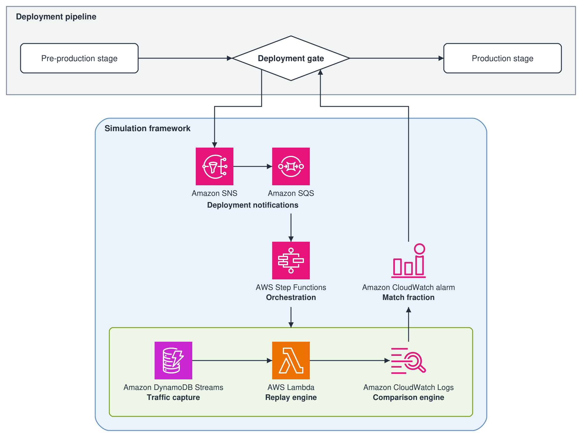
Architecture diagram of the regression testing framework

Figure 1: Regression testing framework architecture

Component insertion flexibility

The framework is designed to be versatile. Each component can be positioned to capture inputs and outputs at any system boundary:

API level: Capture HTTP requests and responses at gateway or service endpoints.
Service level: Capture inter-service communication and message passing.
Database level: Capture query inputs and results for data layer validation.
Message queue level: Capture message processing for event-driven architectures.

You can compare end-to-end outputs or scope the comparison to one block of business logic. Anything after that block, such as formatting or downstream API calls, falls outside the comparison.

Tech stack and rationale

I chose managed AWS services to keep operational overhead low and to pay only for the resources each simulation consumes:

AWS Step Functions: Visual workflow orchestration with built-in error handling and state management for coordinating timed operations.
AWS Lambda: Serverless execution with automatic scaling. Pay only for actual simulation time.
Amazon DynamoDB: Low-latency access to production request data with global tables for multi-Region support. (Note: We used DynamoDB as part of our existing tech stack. You can adapt the framework to the storage system you currently use.)
Amazon CloudWatch: Unified logging, metrics, and alarming. Amazon CloudWatch Logs Insights supports complex queries without additional infrastructure.
Amazon SNS and Amazon SQS: Reliable publish/subscribe messaging for pipeline integration with retry logic and dead-letter queues.

Component 1: Traffic capture – universal storage with complete parameter logging

Core function: Captures actual production request documents and their associated responses, not synthetic data or mocks. This complete production dataset is what makes regression detection accurate by replaying the same requests that flowed through the production system with all their complexity and edge cases.

Key challenge: Capturing all parameters and context needed to reproduce the component’s behavior accurately. Missing any input parameter, request context, or metadata can lead to inaccurate replay and false regression signals.

Apply domain-specific knowledge to identify and capture all inputs your system needs for accurate replay. This includes obvious parameters (request body, headers) and less obvious context (user session state, feature flags, regional settings, timestamps). The completeness of your capture directly determines replay accuracy.

Storage flexibility: The framework design works with any storage system that can generate events:

Amazon DynamoDB Streams: For document-based systems.
Amazon Relational Database Service (Amazon RDS) and Amazon Aurora: Using database triggers or change data capture.
Amazon Kinesis Data Streams: For high-throughput event streaming.
CloudWatch Logs: For API gateway or application-level capture.
Amazon Managed Streaming for Apache Kafka (Amazon MSK): For Kafka-based architectures.

Component 2: Replay engine – running simulated production traffic against test environments

Core function: Takes batched production requests from storage streams and invokes test environment APIs with the same parameters, capturing responses for comparison.

Key challenge: The system needs to distinguish replayed traffic from production traffic. Without this distinction, replayed requests would be processed identically to production requests, leading to duplicate processing and unintended side effects.

The replay engine solves this by attaching simulation IDs to every replayed request:

// Add simulation markers to every replayed request
request.addProperty("simulationId", simulationId);
request.addProperty("isSimulation", true);

Component 3: Comparison engine – domain-specific output analysis

Core function: Compares specific business logic outputs between production and simulation responses to calculate match fractions. The engine extracts the outputs you’ve chosen to focus on and determines whether they match within acceptable thresholds.

Key challenge: Determining what to compare for your specific application. This requires deep domain knowledge. You need to identify which outputs represent your core business logic as opposed to downstream formatting, third-party variations, or environmental differences that do not indicate actual regressions.

Before logging, reduce each response to the fields that carry your business logic, and normalize them so equivalent outputs compare equal, for example by dropping timestamps and sorting lists. The replay engine compares the reduced results and logs one JSON line for each request. Each line has a numeric match field that is 1 when the results are equal and 0 when they differ or the replay fails. Both results stay in the line for investigating mismatches:

{"SimulationId": "<simulationId>", "match": 1, "prod": "<reduced production result>", "sim": "<reduced simulation result>"}

CloudWatch Logs Insights discovers fields in JSON log events, and the query averages match for one simulation:

filter SimulationId = "<simulationId>"
| stats avg(match) as matchFraction

When the replay completes, run the query and publish the match fraction as a custom CloudWatch metric for the deployment gate’s alarm. The implementation reference at the end of this post shows a Lambda function that does this. What constitutes a meaningful comparison depends on your system architecture and business requirements. For the full query language, see the CloudWatch Logs Insights query syntax.

Component 4: Orchestration – CI/CD pipeline integration

Core function: Manages the timing and coordination of simulation components: starts traffic capture, waits for sufficient data collection, stops capture, evaluates results, and provides pass or fail decisions for deployment gates.

Key challenge: Integrating simulation results into continuous integration and continuous delivery (CI/CD) pipelines as reliable quality gates. Deployments need automated pass or fail decisions based on simulation outcomes, not only monitoring data that requires manual interpretation.

Deployment events reach the AWS Step Functions workflow through Amazon SNS, Amazon SQS, and a Lambda function that starts the execution, with retries and error handling.

Replay starts and stops by enabling and disabling the event source mapping between the capture stream and the replay function. Lambda can take several minutes to stop or restart polling after the mapping changes. The workflow waits a few minutes after stopping replay before it evaluates results. When replay is enabled again, the mapping can resume with records captured while it was off. Set a maximum record age on the mapping to skip stale records, and use reserved concurrency on the replay function to cap the burst.

A CloudWatch alarm on the match fraction blocks the deployment when it falls below your threshold. In AWS CodePipeline, for example, an entry condition with a CloudWatchAlarm rule on the production stage blocks promotion while the alarm is in the ALARM state. Otherwise, the pipeline promotes the deployment. The implementation reference at the end of this post shows the state machine definition and the start and stop functions.

Simulation traffic controls and production safety

Critical safeguards prevent overwhelming test environments and maintain production safety:

// Hard limits prevent accidental overload
if (props.trafficFraction > 0.1) throw new Error('Traffic fraction too high');

// Concurrency controls limit resource usage
reservedConcurrentExecutions: 3

Typical configuration: 5 percent traffic replay with 200-record batching provides sufficient coverage while maintaining system stability.

Handling stateful dependencies

As noted in “Scope and applicability,” systems with stateful components can use this framework with additional patterns.

1. Idempotency controls

Services in the simulated logic path can use the simulation IDs described in Component 2 to detect replayed requests. They then skip stateful operations (database writes, notifications, external API calls) while still returning a response.

// Service checks for replay
if (!request.isSimulation()) {
    database.write(result);
    notificationService.send(result);
}

For services that need further isolation, simulation IDs can also be used to route simulation traffic to separate test instances or maintain separate simulation state.

2. Deterministic randomization

For systems using randomization (A/B assignment, sampling, shuffling), use the simulation ID as a seed:

// Production: true randomization
Random rand = new Random();

// Simulation: deterministic based on request
if (request.isSimulation()) {
    rand = new Random(request.getSimulationId().hashCode());
}

This makes simulation responses reproducible and comparable.

When to reconsider

If adding idempotency infrastructure creates an ongoing maintenance burden that exceeds the value of automated regression testing, consider whether this framework is the right fit. Manual testing or alternative validation approaches might be more practical for your system.

Cost and operational efficiency

The framework’s own Lambda functions, logging, streaming, and orchestration cost little. The primary cost driver is your own system processing replayed requests, which varies based on your architecture. The following is a breakdown of the framework costs only. Prices shown are for the US East (N. Virginia) AWS Region as of October 2026. To estimate your own costs, use the AWS Pricing Calculator.

Cost components:

Lambda executions: $0.0000166667 per GB-second plus $0.0000002 per request.
CloudWatch Logs: $0.50 per GB ingested plus $0.03 per GB stored (monthly).
CloudWatch Logs Insights: $0.005 per GB scanned per query.
Step Functions: $0.025 per 1,000 state transitions.
DynamoDB Streams: no read charge when standard AWS Lambda functions read the stream (Lambda Managed Instances incur Streams charges).
Amazon SNS and Amazon SQS: $0.40–$0.50 per million requests.

Example calculation (24-hour simulation, 5 percent of 100,000 daily requests):

5,000 replayed requests × 1 second average duration × 256 MB = about $0.02 Lambda cost.
5,000 log entries × 5 KB average = 25 MB logs = about $0.013 ingestion plus about $0.001 storage.
DynamoDB Streams reads: $0 (included in the preceding Lambda cost).
One evaluation query scanning 25 MB = about $0.0001 Logs Insights.
Step Functions and messaging costs = about $0.01.

Total estimated cost: about $0.05 for this example scenario.

Multi-Region deployment multiplies costs by the number of Regions. Higher traffic volumes scale proportionally. For example, 500,000 daily requests (25,000 replayed) cost approximately $0.25 per simulation.

Scale the calculation based on your traffic volume and simulation frequency. Most importantly, the confidence to deploy faster and the hours saved on manual validation far exceed the simulation costs.

Getting started: Phased implementation approach

Build the framework in three phases. Each phase is usable before the next one starts.

Phase 1 – Core components: Set up traffic capture with your chosen event source, create a replay engine with simulation IDs, implement centralized output analysis with structured logging, and build orchestration with Step Functions.

Phase 2 – Automated verification: Design a match fraction calculation with business logic for filtering variances, create CloudWatch Logs Insights queries, and set up CloudWatch alarms for quality gates.

Phase 3 – Full automation: Integrate with deployment pipelines, deploy across multiple Regions, build monitoring dashboards, and tune thresholds based on real data.

Implementation reference

The following sample code is generalized from my team’s production implementation and is not intended for production use as written. Replace the placeholder names and Amazon Resource Names (ARNs) with your own.

Replay function

@Log4j2
public class ReplayHandler implements RequestHandler<DynamodbEvent, Void> {
    private static final ObjectMapper JSON = new ObjectMapper();
    private final Random random = new Random();
    private final SsmClient ssm = SsmClient.create();
    private final TestServiceClient testService = new TestServiceClient(System.getenv("TEST_ENDPOINT"));

    @Override
    public Void handleRequest(DynamodbEvent event, Context context) {
        SimulationProps sim = SimulationProps.fromJson(
                ssm.getParameter(r -> r.name(System.getenv("SIMULATION_PARAMETER"))).parameter().value());

        for (DynamodbEvent.DynamodbStreamRecord record : event.getRecords()) {
            if (!"INSERT".equals(record.getEventName())) {
                continue;
            }
            CapturedCall captured = CapturedCall.from(record.getDynamodb().getNewImage());
            if (captured.request().isSimulation() || random.nextDouble() > sim.trafficFraction()) {
                continue;
            }
            String prodResult = reduce(captured.response());
            String simResult;
            try {
                simResult = reduce(testService.call(captured.request().withSimulationId(sim.id())));
            } catch (Exception e) {
                simResult = "REPLAY_FAILED: " + e.getMessage();
            }
            log.info(JSON.createObjectNode()
                    .put("SimulationId", sim.id())
                    .put("match", prodResult.equals(simResult) ? 1 : 0)
                    .put("prod", prodResult)
                    .put("sim", simResult)
                    .toString());
        }
        return null;
    }
}

The AWS Systems Manager Parameter Store parameter named in SIMULATION_PARAMETER holds:

{"id": "<execution name>", "trafficFraction": <fraction of traffic to replay>}

CapturedCall, SimulationProps, TestServiceClient, and reduce stand in for your own request model, simulation settings, service client, and response reduction. reduce returns the normalized business-logic fields as a string.

State machine definition

{
  "StartAt": "StartSimulation",
  "States": {
    "StartSimulation": {
      "Type": "Task",
      "Resource": "arn:aws:states:::lambda:invoke",
      "Parameters": {
        "FunctionName": "<start-simulation-function-arn>",
        "Payload": {"id.$": "$$.Execution.Name", "trafficFraction.$": "$.trafficFraction", "durationSeconds.$": "$.durationSeconds"}
      },
      "OutputPath": "$.Payload",
      "Catch": [{"ErrorEquals": ["States.ALL"], "ResultPath": "$.error", "Next": "StopSimulation"}],
      "Next": "WaitForSimulation"
    },
    "WaitForSimulation": {
      "Type": "Wait",
      "SecondsPath": "$.durationSeconds",
      "Next": "StopSimulation"
    },
    "StopSimulation": {
      "Type": "Task",
      "Resource": "arn:aws:states:::lambda:invoke",
      "Parameters": {"FunctionName": "<stop-simulation-function-arn>", "Payload.$": "$"},
      "OutputPath": "$.Payload",
      "Next": "WaitForInFlightReplays"
    },
    "WaitForInFlightReplays": {
      "Type": "Wait",
      "Seconds": 300,
      "Next": "EvaluateSimulationResults"
    },
    "EvaluateSimulationResults": {
      "Type": "Task",
      "Resource": "arn:aws:states:::lambda:invoke",
      "Parameters": {
        "FunctionName": "<evaluate-simulation-results-function-arn>",
        "Payload": {"id.$": "$$.Execution.Name", "simulationStartTime.$": "$$.Execution.StartTime"}
      },
      "End": true
    }
  }
}

Start and stop functions

import {LambdaClient, UpdateEventSourceMappingCommand} from "@aws-sdk/client-lambda"
import {PutParameterCommand, SSMClient} from "@aws-sdk/client-ssm"

const lambda = new LambdaClient({})
const ssm = new SSMClient({})

const setReplayEnabled = (enabled: boolean) =>
    lambda.send(new UpdateEventSourceMappingCommand({
        UUID: process.env.REPLAY_LAMBDA_TRIGGER_UUID,
        Enabled: enabled,
    }))

export const startSimulation = async (event: {id: string; trafficFraction: number; durationSeconds: number}) => {
    await ssm.send(new PutParameterCommand({
        Name: process.env.SIMULATION_PARAMETER,
        Value: JSON.stringify({id: event.id, trafficFraction: event.trafficFraction}),
        Type: "String",
        Overwrite: true,
    }))
    await setReplayEnabled(true)
    return event
}

export const stopSimulation = async (event: object) => {
    await setReplayEnabled(false)
    return event
}

Evaluation function

import {CloudWatchLogsClient, GetQueryResultsCommand, StartQueryCommand} from "@aws-sdk/client-cloudwatch-logs"
import {CloudWatchClient, PutMetricDataCommand} from "@aws-sdk/client-cloudwatch"

const logs = new CloudWatchLogsClient({})
const cloudwatch = new CloudWatchClient({})

const matchFractionQuery = (simulationId: string) =>
    `filter SimulationId = "${simulationId}" | stats avg(match) as matchFraction`

const publishMatchFraction = (value: number) =>
    cloudwatch.send(new PutMetricDataCommand({
        Namespace: "RegressionSimulation",
        MetricData: [{MetricName: "MatchFraction", Value: value, Unit: "None"}],
    }))

export const handler = async (event: {id: string; simulationStartTime: string}) => {
    const {queryId} = await logs.send(new StartQueryCommand({
        logGroupName: process.env.REPLAY_LOG_GROUP,
        startTime: Math.floor(Date.parse(event.simulationStartTime) / 1000),
        endTime: Math.floor(Date.now() / 1000),
        queryString: matchFractionQuery(event.id),
    }))

    let result
    do {
        await new Promise((resolve) => setTimeout(resolve, 5000))
        result = await logs.send(new GetQueryResultsCommand({queryId}))
    } while (result.status === "Scheduled" || result.status === "Running")

    const value = result.results?.[0]?.find((field) => field.field === "matchFraction")?.value
    if (result.status !== "Complete" || !value) {
        await publishMatchFraction(0)
        throw new Error(`Simulation ${event.id} produced no match fraction (query status ${result.status})`)
    }

    const matchFraction = parseFloat(value)
    await publishMatchFraction(matchFraction)
    return {simulationId: event.id, matchFraction}
}

Conclusion

This component-based simulation framework transformed our deployment process from manual and time-intensive to automated and reliable, saving hours per deployment while achieving high accuracy in regression detection. The modular design means the same building blocks can be inserted anywhere in your system architecture to validate that code changes do not break existing functionality.

Look at how your team catches regressions today. If refactors, dependency upgrades, or feature-flagged releases reach production with only synthetic test coverage, or if regressions surface first in post-deployment alarms, replaying production traffic before deployment closes that gap. Start with one stateless component, such as a pricing or validation engine, where replay needs no changes to your service code.

To get started, see the AWS Step Functions detail page and the AWS Step Functions Developer Guide. This framework also uses AWS Lambda, Amazon DynamoDB, Amazon CloudWatch, Amazon SNS, and Amazon SQS.

About the author

Scale distributed AI workloads with Ray and Anyscale on Amazon EC2

2026-11-12 Sindhura Palakodety

Post Syndicated from Sindhura Palakodety original https://aws.amazon.com/blogs/architecture/scale-distributed-ai-workloads-with-ray-and-anyscale-on-amazon-ec2/

If you are building multimodal artificial intelligence and machine learning (AI/ML) pipelines on Amazon Elastic Compute Cloud (Amazon EC2) that process text, video, and audio, you have likely hit at least one of these challenges. Scaling from a single instance to distributed compute without rewriting code, managing costs across training, fine-tuning, and inference, and keeping up with an evolving network of models, frameworks, and hardware are among the biggest challenges AI engineers face today. These challenges compound when each pipeline stage has distinct compute, networking, and storage requirements, and multiple teams own separate parts of the workflow.

This post shows how the Ray-powered Anyscale application on AWS helps you tackle these challenges. You will learn how to: deploy Ray across three AWS compute options based on your operational requirements, optimize costs by matching heterogeneous instance types to each pipeline stage, and scale from prototype to production without code changes.

How Anyscale builds on Ray

Ray Core is the distributed computing foundation underlying the entire framework. It provides primitives for parallelizing Python workloads across clusters, handling task scheduling, fault tolerance, and autoscaling. Ray AI libraries are built on top of Ray Core. As a result, custom workloads that don’t fit a standard pattern can still use the same distributed infrastructure.

Ray Data ingests and transforms datasets at scale, feeding processed data into training, tuning, and inference stages. Ray Train orchestrates distributed multi-node jobs with built-in fault tolerance, supporting foundation model fine-tuning across architectures such as Llama and Mistral with automatic selection of data-parallel, model-parallel, or pipeline-parallel strategies. Ray Tune parallelizes hyperparameter experiments across large clusters. Ray Serve runs production inference endpoints with dynamic batching, automatic scaling, and multi-model deployment support. Ray RLlib supports distributed reinforcement learning workloads, including reinforcement learning from human feedback (RLHF) for large language model (LLM) alignment.

Anyscale on AWS

Many AWS customers already run self-managed Ray clusters on Amazon EC2. Anyscale builds on that foundation as a fully managed service that deploys within your AWS account, integrating with your existing Amazon Virtual Private Cloud (Amazon VPC) networks, AWS Identity and Access Management (IAM) roles, and compliance frameworks. The application handles cluster management, autoscaling, and cost controls so you can focus on workloads rather than infrastructure.

AWS and Anyscale together address three dimensions of production AI/ML: cost-efficient infrastructure spanning the full Amazon EC2 portfolio, a Ray-on-Anyscale stack that scales reliably from experimentation to production, and an integrated framework that reduces friction at every stage of development. With Anyscale, you can map each pipeline stage to the appropriate instance type. Intel and AMD-based instances handle preprocessing, tokenization, and feature extraction. AWS Graviton-based instances cover preprocessing, worker nodes, embedding generation, and lightweight inference where price-performance matters. NVIDIA GPU instances and AWS Trainium handle training and fine-tuning. AWS Inferentia serves high-throughput inference endpoints. Amazon EC2 Spot Instances run automatically for batch training, preprocessing, and hyperparameter sweeps.

Anyscale deployment architecture on AWS

Three deployment options provide flexibility based on operational requirements:

Amazon EC2 with Elastic Fabric Adapter (EFA) provides direct compute control and high-performance inter-node networking.

Amazon Elastic Kubernetes Service (Amazon EKS) with EFA supports containerized workloads.

Amazon SageMaker HyperPod delivers managed large-scale foundation model training with built-in cluster resiliency.

Regardless of the deployment path, Ray libraries handle distinct pipeline stages. Ray Data orchestrates preprocessing across CPU-only instances, AWS Graviton-based instances, GPU instances, and Spot Instances. Ray Train, Ray Serve, and Ray RLlib handle distributed training, inference serving, and reinforcement learning on NVIDIA GPU instances and AWS AI chips.

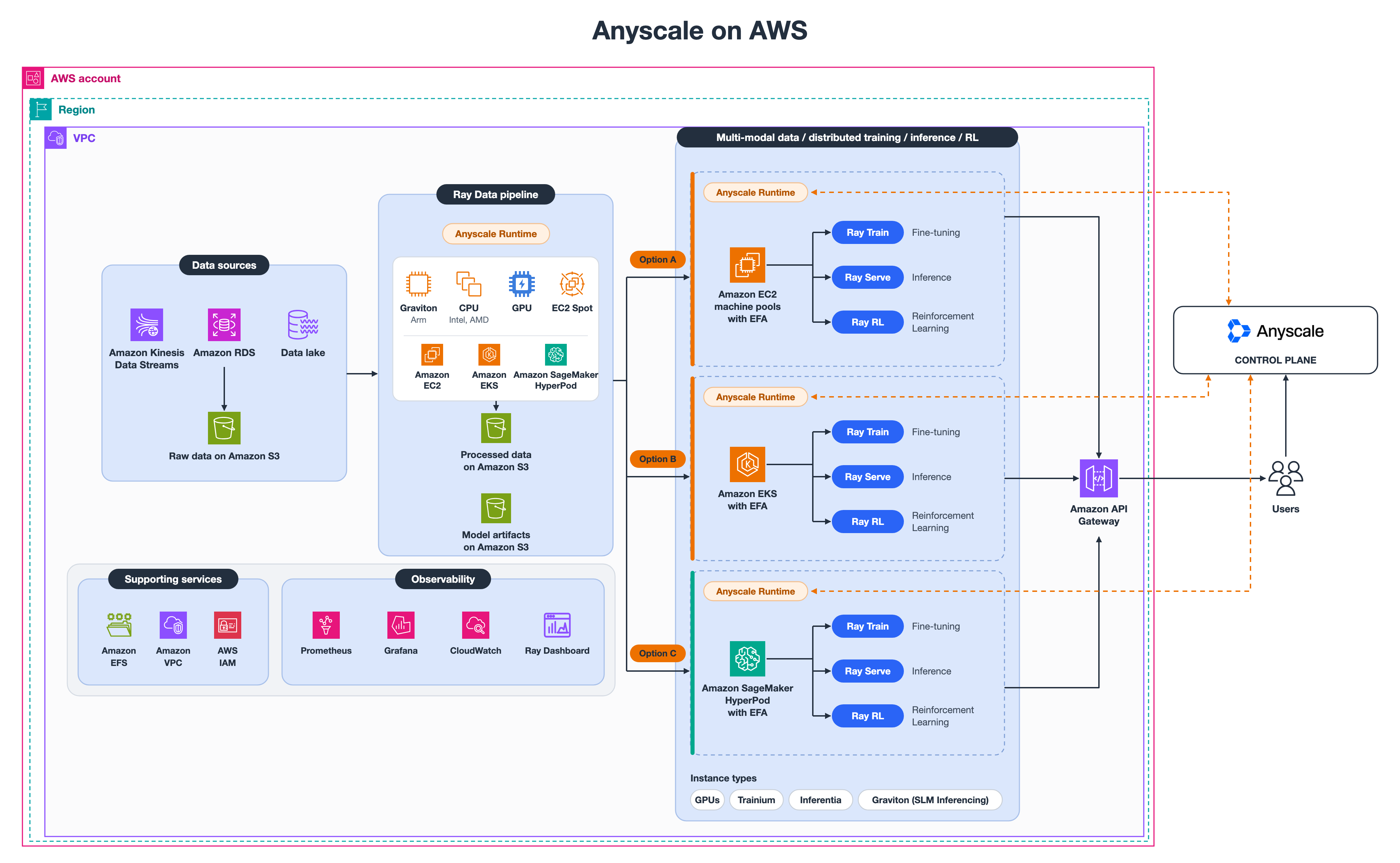
Reference architecture showing the Anyscale on AWS solution deployed across multiple AWS services

Figure 1: Anyscale on AWS architecture

Anyscale runs a hosted control plane that sends instructions to an operator deployed in your AWS environment. The data plane (Amazon EC2 instances, storage, and networking) stays in your account, and Anyscale manages Ray cluster lifecycle without direct access to your data.

Option A: Amazon EC2

Amazon EC2 supports the full pipeline without constraint. This makes it the recommended default for teams running EC2-based workloads who want to scale into AI/ML without retooling their operations. Ray Data runs preprocessing on cost-efficient instance types including Spot Instances and Graviton processors. Ray Train handles distributed training on GPU and Trainium instances with EFA. Ray Tune runs hyperparameter search across CPU and GPU instances. Ray Serve deploys inference on Inferentia or Graviton. Ray supports reinforcement learning through RLlib on GPU instances, and RLHF workflows run through frameworks such as OpenRLHF.

Anyscale manages instance lifecycle, provisioning and terminating nodes based on demand. Amazon Simple Storage Service (Amazon S3) handles datasets, checkpoints, and model artifacts. Amazon FSx for Lustre provides parallel file system throughput for training jobs with repeated large-dataset reads. EFA is available on supported instance types for multi-node training.

Option B: Amazon EKS

Amazon EKS runs the same full pipeline within a Kubernetes environment. This makes it the right choice if your organization already manages Kubernetes and wants Ray to share the same infrastructure and tooling. The Anyscale operator deploys Ray nodes as pods, and Ray libraries run identically to the Amazon EC2 path at the application layer.

Karpenter handles node autoscaling, provisioning GPU nodes for training, Graviton nodes for preprocessing and inference, and Spot Instances for batch workloads. Ray Serve benefits from Kubernetes-integrated zero-downtime upgrades for production inference deployments. The tradeoff: Amazon EKS adds container orchestration complexity and requires custom configuration for the Anyscale operator.

Option C: Amazon SageMaker HyperPod

Amazon SageMaker HyperPod is purpose-built for resilience-critical stages where multi-week runs on large GPU or Trainium clusters make node failures expensive. It continuously monitors cluster health, automatically replaces unhealthy nodes, and resumes from the last checkpoint without manual intervention. HyperPod supports both Slurm-orchestrated and Amazon EKS-based clusters, and now supports the full model development lifecycle including inference deployment. Amazon SageMaker Studio integration adds experiment tracking and model management.

Native integrations shared by EC2, EKS, and HyperPod

Networking and storage

EFA provides low-latency, high-bandwidth inter-node communication for distributed training on all three deployment paths. Amazon S3 is the primary store for datasets, checkpoints, and artifacts. Ray Data pipelines read directly from Amazon S3-based data lakes. Amazon FSx for Lustre integrates with S3 for parallel file system throughput. Amazon Elastic File System (Amazon EFS) covers shared file access for workspaces and notebooks.

Security and compliance

Amazon Virtual Private Cloud (Amazon VPC) network isolation, IAM role-based access control, and AWS Key Management Service (AWS KMS) encryption at rest and in transit apply regardless of deployment path. Data stays within your AWS account and encryption keys remain under your control. This architecture supports compliance with frameworks including HIPAA and SOC 2 without changes to Ray workload code.

Observability

Anyscale monitoring provides workload-specific dashboards covering training progress, pipeline throughput, and request latency. Grafana dashboards are accessible from the Anyscale console. Amazon CloudWatch handles AWS metrics, logs, and alarms. Prometheus supports custom metrics collection for teams with existing monitoring pipelines.

Each deployment path follows the same workflow: Ray Data feeds processed data to Anyscale Runtime, Ray Train orchestrates training, Ray Serve handles inference through Amazon API Gateway, and Ray RLlib supports reinforcement learning.

Cost optimization and provisioning

Right-sizing compute per stage

AWS Graviton-based instances deliver strong price-performance for CPU-bound Ray workloads across preprocessing, embedding generation, and lightweight inference. PyTorch inference on Graviton3 C7g instances shows up to 50% cost savings versus x86 equivalents (Tomaz Berisa, n.d.). Graviton4 adds 30% better compute per core and 75% more memory bandwidth than Graviton3 (AWS, n.d.). Graviton also runs small language models (1–7B parameters) cost-efficiently for generative AI inference.

Intel-based instances provide strong x86 price-performance for tokenization, batch transforms, and workloads requiring broad framework compatibility. AMD-based instances deliver strong performance for CPU-intensive preprocessing, feature engineering, and inference workloads requiring maximum throughput per core. NVIDIA GPU instances provide high throughput for distributed training, fine-tuning, and large-model inference.

AWS Trainium2 delivers 30–40% better price-performance than comparable GPU instances for training at scale (AWS, n.d.). AWS Inferentia2 provides up to 4x higher throughput and 10x lower latency than its predecessor for production inference. Ray auto-detects accelerator types, so Anyscale routes each workload stage to the appropriate hardware without manual configuration.

Spot Instances with Ray fault tolerance

Anyscale keeps head nodes on On-Demand and runs workers on Spot with automatic fallback. Ray Data retries failed tasks on replacement nodes. Ray Train resumes from checkpoints, achieving up to 60% savings on distributed training. Ray Serve proactively migrates replicas on the 2-minute preemption warning.

Capacity Blocks and On-Demand Capacity Reservations

For scheduled training runs requiring capacity availability, Amazon EC2 Capacity Blocks reserve 1–64 accelerated instances for up to six months, bookable eight weeks in advance. Each block supports up to 512 GPUs or 1,024 Trainium chips, placed in Amazon EC2 UltraClusters with petabit-scale networking. Anyscale machine pools reference capacity reservations directly with priority-ordered fallback: Capacity Block, then Spot, then On-Demand. On-Demand Capacity Reservations (ODCRs) provide open-ended capacity availability.

Combined provisioning strategy

Anyscale runs two-layer autoscaling: Ray Serve scales replicas on request metrics while the cluster autoscaler provisions and terminates nodes. The recommended purchasing stack starts with AWS Compute Savings Plans, saving up to 66% across Graviton, GPU, Trainium, and Inferentia. Layer on Spot for fault-tolerant batch jobs, Capacity Blocks for scheduled training, and On-Demand for burst.

Getting started: From prototype to production

Your path follows four phases, each building on the last without code changes:

Phase 1: Validate locally (1–2 days). Start with Ray on a single Amazon EC2 instance or your laptop. Build your data pipeline and training loop, and validate model quality before touching distributed infrastructure.

Phase 2: Scale data (1–2 weeks). Deploy Ray Data with AWS Graviton and Amazon EC2 Spot Instances to process your full dataset at scale, with Spot Instances reducing preprocessing costs by up to 90% (AWS, n.d.).

Phase 3: Scale training (2–4 weeks). Choose your deployment option: Amazon EC2 for maximum flexibility, Amazon EKS for Kubernetes-native environments, or Amazon SageMaker HyperPod for resilience-critical runs. Scale training across multiple GPUs or AWS Trainium instances with EFA.

Phase 4: Deploy inference (1–2 weeks). Deploy Ray Serve for model serving with autoscaling configured to your traffic patterns.

The same code runs across all four phases. Moving from a single instance to a multi-node cluster requires only configuration changes managed by Anyscale.

Conclusion

Ray and Anyscale on AWS provide a practical path from prototype to production across the full AI/ML pipeline. Three deployment options address different operational requirements: Amazon EC2 for maximum flexibility, Amazon EKS for Kubernetes-native environments, and Amazon SageMaker HyperPod for resilience-critical training. With heterogeneous clusters mixing Amazon EC2 Spot Instances, AWS Graviton, NVIDIA GPUs, AWS Trainium, and AWS Inferentia, you can match compute to each pipeline stage. The same Ray code runs from a single instance to a multi-node cluster without modification, and Anyscale handles cluster management, fault tolerance, autoscaling, and resource orchestration.

Your next steps depend on where you are today:

Already running Ray on AWS – deploy Anyscale through the AWS Marketplace for managed autoscaling, cost controls, and governance.
New to distributed ML – start with the Anyscale documentation on a single Amazon EC2 instance, then scale out.
Evaluating Anyscale – explore the Ray quickstart for architecture guides and tutorials.

For more on the AWS services covered in this post, see the documentation for Amazon EC2, Amazon EKS, Amazon SageMaker HyperPod, AWS Trainium, AWS Inferentia, and AWS Graviton.

About the authors

Per-customer invoice management with Amazon EventBridge Scheduler

2026-11-12 Rana Kiziltoprak German

Post Syndicated from Rana Kiziltoprak German original https://aws.amazon.com/blogs/compute/per-customer-invoice-management-with-amazon-eventbridge-scheduler/

Many software as a service (SaaS) platforms need to bill each customer on their unique billing cycle, based on the date they signed up. This creates a complex scheduling problem: an individually timed invoice generation event per customer, each followed by precisely timed payment reminders. On a large platform, that adds up to millions of events.

In this post, we show you how to use Amazon EventBridge Scheduler as the time-aware backbone of a per-customer billing system. You learn how to create recurring schedules for invoice generation, spawn one-time schedules for payment reminders, and manage the full customer billing lifecycle, all without building or operating scheduling infrastructure.

Overview

This solution uses the following AWS services:

Amazon EventBridge Scheduler: Manages the per-customer recurring and one-time schedules.
AWS Lambda: Runs the invoice generation and reminder logic.
Amazon Simple Email Service (Amazon SES): Sends the invoice and reminder email.
Amazon DynamoDB: Stores the reminder log that makes reminder delivery idempotent.
Amazon Simple Queue Service (Amazon SQS): Provides the dead-letter queue for failed invocations.

Prerequisites

To follow along with this post, you need:

An AWS account.
The AWS Command Line Interface (AWS CLI) configured with appropriate credentials.
Python 3.12 or later with Boto3. Python 3.9 has reached end of support as a Lambda runtime, so use a current runtime for new functions.
An AWS Identity and Access Management (IAM) role with permissions to create Amazon EventBridge Scheduler schedules and invoke Lambda functions.
A DynamoDB table named billing-reminder-log with idempotency_key as its partition key, and time to live (TTL) enabled on the ttl attribute so that old reminder records expire on their own.
A verified sending identity in Amazon SES. If your account is still in the SES sandbox, request production access before you send to arbitrary customer addresses, because the sandbox only allows sending to verified addresses.
An SQS queue to use as the dead-letter queue for failed schedule invocations.

The problem

You run a SaaS platform. Each customer signs up on a different day, and their billing cycle starts from that signup date. Customer A signed up on March 3, so they get invoiced on the 3rd of every month. Customer B signed up on the 17th, and they get invoiced on the 17th. You have 500,000 customers, each with their own billing anchor date.

Now layer on payment reminders: 7 days before the invoice is due, 3 days before, and the day it is due. That is four scheduled actions per customer per billing cycle, which comes to millions of events every month.

How do you build this?

The traditional approach (and why it breaks)

Most teams consider one of these patterns:

A cron job that scans the database every hour: Query all customers, check whether anyone is due for an invoice or a reminder, and process them. This works at small scale but becomes a bottleneck fast. The job takes longer as your customer base grows. If it crashes mid-run, you miss invoices. If it runs slowly, reminders arrive late.
A queue with delayed messages: An appealing idea at first glance, but Amazon SQS caps DelaySeconds at 15 minutes (900 seconds), which rules it out for billing events scheduled days or weeks ahead.

Both approaches share the same drawback: you are building and operating scheduling infrastructure instead of focusing on your billing product.

The building block: Amazon EventBridge Scheduler

Amazon EventBridge Scheduler is purpose-built for this problem. It is a fully managed scheduling service that handles billions of one-time and recurring invocations. You create a schedule, tell it when to fire and what to invoke, and walk away. There is no infrastructure to manage, no polling, and no worker fleets.

For per-customer billing, Scheduler becomes the time-aware backbone of your invoicing system:

Each customer gets their own recurring schedule for invoice generation.
Each billing cycle spawns one-time schedules for payment reminders.
Scheduler handles the timing, and your application handles the business logic.

Architecture

The following diagram shows the end-to-end flow, from customer signup through invoice generation and payment reminders.

At signup, the application creates a recurring monthly schedule for the customer’s signup day. On each billing day, this schedule invokes the invoice generation Lambda function. The function sends the invoice through Amazon SES and sets up three one-time payment reminders: 7 days before the due date, 3 days before, and on the due date. Each reminder invokes the Send Payment Reminder Lambda function, which notifies the customer only if the invoice is still unpaid. When a payment arrives, a separate handler deletes any outstanding reminders so no further messages go out.

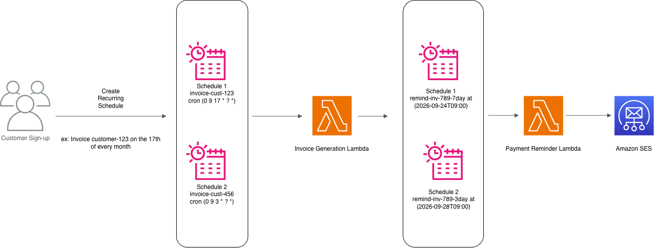
Figure 1: Invoice generation and payment reminders with Amazon EventBridge Scheduler

Implementation

The complete implementation is available in the accompanying GitHub repository. The AWS Serverless Application Model (AWS SAM) template provisions the DynamoDB tables, SQS dead-letter queue, Amazon EventBridge Scheduler groups, AWS Key Management Service (AWS KMS) key, and AWS Lambda functions described in this section. The rest of this section walks through the design of each component.

Step 1: Create schedule groups

Before creating any schedules, make sure the schedule groups exist. The sample declares them in the AWS SAM template so they are provisioned once at stack deploy time.

When a customer signs up, the signup handler creates a recurring schedule based on their signup date. For customers who sign up on the 29th, 30th, or 31st, the sample clamps the billing day to the last day of each month using the L cron special character, so no customer is skipped in February or in 30-day months. The handler is idempotent: if the schedule already exists (for example, after a retry), it updates the schedule instead of failing.

Step 3: Generate the invoice and schedule reminders

The invoice generation Lambda function, GenerateInvoice, does the billing work and then creates one-time schedules for the payment reminders. It includes an idempotency check to prevent duplicate invoices if Scheduler delivers the event more than once.

Step 4: Send reminders with idempotency

The reminder Lambda function, SendPaymentReminder, checks whether the invoice is still outstanding and whether this specific reminder was already sent, which prevents duplicate reminders on retry.

Step 5: Cancel reminders on payment (event-driven)

Instead of checking payment status only when a reminder fires, a payment handler cancels outstanding reminders immediately when a payment is received. Your payment processing system triggers this handler (for example, through an Amazon EventBridge event or an SQS message from your payment gateway).

Step 6: Handle customer lifecycle changes

When a customer cancels, upgrades, or changes their billing cycle, update or delete their schedule accordingly. One thing to be careful of: UpdateSchedule replaces the entire schedule configuration rather than merging changes, so any field you leave out is lost. Always read the existing schedule first, then apply your changes and write it back in full.

Why Scheduler is the right building block

The following table compares the do-it-yourself (DIY) approach with Amazon EventBridge Scheduler for each operational concern.

Concern	DIY Approach	With Scheduler
Per-customer timing	Complex database queries to find who is due	Each customer has their own schedule, so no queries are needed
Reminder precision	Polling interval determines accuracy	Fires at the minute you specify, within the flexible time window you configure
Scale	More customers = more polling load, more workers	Scheduler handles millions of schedules natively
Missed executions	Crashed cron host = missed invoices	Fully managed, built-in retries with a dead-letter queue
Early payment	Reminders fire anyway, or you build cancellation logic into your poller	Delete the schedule and it does not fire
Lifecycle changes	Update database records, hope the poller picks up the change	Update or delete the schedule directly
Operational overhead	Manage worker fleets, monitor queue depth, handle clock skew	Zero infrastructure to manage

Operational considerations

Before you run this design in production, consider the following operational factors.

Schedule groups for organization

Use schedule groups to organize and manage schedules by function:

billing-invoices: All recurring invoice generation schedules.
billing-reminders: All one-time payment reminder schedules.

With schedule groups, you can tag a set of schedules for organization and access control, list schedules by category, and delete all schedules in a group if needed (for example, during testing).

Quotas and request rates at scale

Service quotas matter once you move past a test account. One quota is the number of schedules. The default limit is 10 million schedules per account per Region, and it is adjustable through Service Quotas. The CreateSchedule and UpdateSchedule APIs also have request rate quotas, which matters if you backfill existing customers in a single migration. Spread that backfill over time if you do not need to backfill immediately.

Scheduler also throttles invocations, with a default of 500–1,000 transactions per second (TPS) depending on the Region and adjustable to tens of thousands of TPS. To deal with an invocation spike (for example, the majority of your customers having invoices due at the same time), we recommend using the Flexible Time Window feature. In this post, we use it to spread each burst over 15 minutes, which smooths the load on your downstream Lambda functions and on Amazon SES without changing what the customer sees on their invoice.

Monitoring

Monitor schedule health with Amazon CloudWatch metrics, and capture any failed invocations in a dead-letter queue.

CloudWatch metrics: Monitor InvocationAttemptCount, InvocationDroppedCount, InvocationThrottleCount, and TargetErrorCount per schedule group.
Dead-letter queue: Configure a dead-letter queue on your schedules to capture failed invocations that exhaust retries, and alarm on the InvocationsSentToDeadLetterCount metric so a failed delivery pages you instead of sitting silent in the queue.
Invoice audit trail: Log every invoice generation and reminder send to an Amazon DynamoDB table or Amazon CloudWatch Logs for compliance.

Retry policy

The retry policy and dead-letter queue are applied to every schedule target the sample creates. This retries transient Lambda failures up to three times over 1 hour, and permanently failed invocations land in the SQS dead-letter queue for investigation.

Cost at scale

Amazon EventBridge Scheduler pricing is based on invocations, and the AWS Free Tier covers 14 million invocations per month. The 500,000-customer example in this post generates four scheduled events per customer per month (one invoice and three reminders), which is 2 million invocations, so the scheduling layer costs nothing at that scale. Scale the same design to 10 million customers and you generate 40 million invocations per month, of which 26 million are billable at $1.00 per million, so the scheduling layer costs roughly $26 per month.

The costs that grow with this design sit in the targets rather than in the scheduling:

AWS Lambda charges for each invocation and its duration.
Amazon SES charges per email, so the three reminders per customer per cycle are the largest line item in this workload.
Amazon DynamoDB charges for the reminder log writes and reads, which the TTL setting keeps from accumulating.

Check the pricing page for each service for current rates in your AWS Region.

Cleanup

To avoid incurring charges, delete the resources you created. If you deployed the accompanying SAM sample, run sam delete --stack-name <stack-name>, which removes the Lambda functions, DynamoDB tables, SQS queue, KMS key, and IAM roles in one command. Before deleting the stack, delete any schedules the sample created at runtime, because schedule groups cannot be deleted while they still contain schedules. If you deployed the resources manually, delete them in this order:

Delete the schedule groups. Deleting a group also deletes the schedules it contains.
Delete the Lambda functions (GenerateInvoice and SendPaymentReminder).
Delete the IAM roles (SchedulerInvoiceRole and SchedulerReminderRole).
Delete the SQS dead-letter queue.
Delete the billing-reminder-log DynamoDB table.

Conclusion

Billing is inherently time-driven. Every customer has a cycle, every invoice has a due date, and every reminder has a send time. When you build billing infrastructure, you are building scheduling infrastructure whether you set out to or not.

With Amazon EventBridge Scheduler, you can stop building scheduling infrastructure and focus on your billing logic. Each customer’s billing lifecycle becomes a set of schedules, created at signup, updated when plans change, and deleted at cancellation. The timing is managed for you, the service scales to millions of schedules per Region, and the operational burden of running the scheduler moves to AWS.

If your application has per-customer timing, Scheduler is the building block that makes it straightforward.

To deploy this solution, use the accompanying AWS SAM project on GitHub, which provisions the Lambda functions, DynamoDB tables, Amazon EventBridge Scheduler groups, and SQS dead-letter queue described in this post. For more information about the service, see the Amazon EventBridge Scheduler documentation and the Amazon EventBridge Scheduler product page. For more serverless learning resources, visit Serverless Land.

About the authors

Inside an enterprise AI agent: A governed, observable loop architecture

2026-11-12 Rushabh Lokhande

Post Syndicated from Rushabh Lokhande original https://aws.amazon.com/blogs/architecture/inside-an-enterprise-ai-agent-a-governed-observable-loop-architecture/

An enterprise AI agent isn’t a bigger chatbot. A chatbot answers one message at a time. An agent keeps working toward a goal: it reads what the user is asking for, breaks the work into steps, pulls in the knowledge it needs, weighs the evidence, calls external tools, and checks the results before it decides whether to keep going or hand back an answer. Every one of those steps touches real systems and real data, so governance, observability, and trust controls must live at each step. Most chatbot designs don’t provide them.

This post lays out a reference architecture for that kind of agent, organized as five layers: an API gateway that handles identity and policy, a five-phase agent runtime (Understand, Plan, Retrieve, Reason, and Act and Observe), a knowledge and state tier that gives the agent memory, a platform-services layer for models and tools, and a trust and control framework that runs across all of them. Each layer maps to AWS managed services. We also cover the design patterns that work and the mistakes we have seen teams make.

The rise of enterprise AI agents

Enterprises are moving past single-turn question-and-answer interfaces for business reasons. They want to automate more of the routine work so their people can spend time elsewhere, ship products and customer experiences faster, and get more done without adding headcount. Those goals justify the investment, but reaching them requires moving from single-turn chatbots to agents that can carry out multi-step work on their own. That jump brings new problems to solve in orchestration, memory, and governance, and the rest of this section is about what those problems demand of the architecture.

From chatbots to agents

Enterprise AI is shifting from systems that answer a question and stop to agents that plan, use tools, and come back with an outcome you can verify. The difference is the loop. Rather than returning one response, an agent cycles through understanding, planning, retrieval, reasoning, and action, and it keeps cycling until it either reaches the user’s goal or decides a human needs to step in.

At AWS re:Invent 2025, Werner Vogels said that the developers who succeed think in systems and build with precision. The teams pulling ahead with agents aren’t the teams that moved first or chose the newest model. They are the ones who treat the whole thing as a system and understand that a choice made in one layer shows up in every layer around it.

What is an AI agent? An AI agent uses a foundation model (FM) as its reasoning core and adds tools, memory, and guardrails so it can take on work that takes more than one step. Where a single-turn chatbot answers and forgets, an agent holds onto state, reasons across several steps, and acts in systems outside itself.

The enterprise imperative: Governed, observable, trustworthy, cost-aware

A capable model is the more straightforward part. Running agents in an enterprise means putting governance, observability, trust controls, policy enforcement, and cost controls around every step they take. Cost matters as much as capability: many enterprises find token spend growing faster than the productivity gains it delivers, so an agent must also be designed to spend inference where it adds value. That is what this architecture is built to do:

Governed – Every action clears a policy gate, an approval workflow, or a guardrail before it runs.
Observable – Each step emits a trace (latency, tokens, tool status, and execution path) for later audit.
Trustworthy – Confidence scoring, evaluations, and human checkpoints sit between the agent and the user.
Iterative – The loop sharpens its understanding on each pass as tool results come back.

What this post covers

What follows is a reference architecture for enterprise AI agents on AWS, walked through layer by layer from the first request to the verified result, with diagrams, the AWS services that implement each piece, and the patterns worth copying and avoiding. The aim is to give architects and engineering leaders a shared vocabulary and a mental model for designing these systems.

Architecture overview: The governed agent loop

The AWS Well-Architected Framework Generative AI Lens organizes generative AI workloads around six pillars (operational excellence, security, reliability, performance efficiency, cost optimization, and sustainability), each with its own practices and controls. We split the agent into layers that line up with those pillars, so every layer owns a clear responsibility that traces back to a recognized standard instead of a one-off choice. Teams can change, secure, and scale one layer without disturbing the others while keeping the end-to-end governance the Lens requires.

Layered architecture design

The design is layered and loop-based, with five tiers that each do one job. The agent runtime sits in the middle. It’s a five-phase loop that turns a user’s goal into a verified outcome. Around it sit the layers for knowledge, platform services, trust controls, and the governance that cuts across everything.

Reference architecture diagram

Figure 1 shows the five layers together. Read it top to bottom: the API gateway takes the request and enforces identity and policy, then the flow moves down through the agent runtime, the knowledge and state tier, and the platform services, with the trust and control framework running alongside on the right.

Five-layer enterprise AI agent reference architecture: API gateway, agent runtime, knowledge and state, platform services, and a cross-cutting trust and control framework

Figure 1: Inside an enterprise AI agent, reference architecture

Design principles

Five principles shaped this design, and each one left a mark on the layers you will see later in concrete ways. Zero trust is why identity context travels through every phase of the loop. Observable by default is why there is a dedicated step-level tracing tier instead of leaning on application logs.

These principles aren’t ad-hoc. They come directly from the AWS Well-Architected Framework Generative AI Lens. The Lens’s security guidance maps closely to the following five principles. Least-privilege access across models, data stores, endpoints, and workflows is what zero trust and defense in depth rest on. Securing the data and the traffic between components is separation of concerns in practice. Watching and enforcing the boundaries between the control and data planes is observable by default doing its job. And constraining what the agent is allowed to do, through guardrails and clear limits, is where fail-safe defaults come from. Because it builds on the Lens, this design follows recognized AWS guidance rather than a single team’s convention. It also reflects what AWS Professional Services has implemented and run in production with enterprise customers across industries such as retail and technology: lessons learned in the field that we apply on every engagement, not a set of theoretical best practices. For the full security guidance, see the Generative AI Lens security pillar in the AWS Well-Architected documentation.

Principle	Description
Zero trust	Every request is authenticated and authorized before reaching the runtime. User identity flows through every phase.
Defense in depth	Multiple layers of controls (API gateway, policy gate, trust and control, governance) facilitate no single point of failure.
Separation of concerns	Each architectural layer has clear boundaries and responsibilities. Knowledge is separated from compute. Trust is separated from execution.
Observable by default	Every step produces telemetry. Tracing, metrics, and logs are first-class architectural concerns, not afterthoughts.
Fail-safe defaults	When uncertain, the agent defaults to the safest action: clarify with the user or escalate to a human.

Entry point: User goal and API gateway, identity and policy

Layer 1 of 5 · Entry point: API gateway, identity, and policy (see Figure 1)

Every interaction starts with a user goal: a request in plain language that kicks off the loop. Before it reaches the runtime, it goes through the API gateway and the identity and policy layer, where the zero-trust posture is enforced.

User goal

The user goal starts with a business objective that drives the top-level intent, stated in natural language. It might be as small as “What was our Q3 revenue?” or as involved as “Book a meeting with Sarah, check her calendar availability, and send a summary of our last project discussion.” The agent’s first job is to read that intent and work out the most efficient way to deliver it.

API gateway

The API gateway is the front door for every interaction. It terminates TLS, routes requests (REST, plus WebSocket for streaming responses), applies rate limits, and validates input. On AWS, this is usually Amazon API Gateway with WebSocket APIs for real-time streaming.

Identity and authentication

No request reaches the runtime unauthenticated. The identity layer checks OAuth 2.0 / OpenID Connect (OIDC) tokens, resolves who the caller is, and attaches their context (role, permissions, organization, and session ID) to the request. That context rides along through every later phase, so each tool call and data lookup stays within the caller’s permissions.

Policy enforcement

The policy layer handles role-based access control (RBAC), tool-level permissions, data scoping, and usage quotas. It decides which tools the agent might call for a given user, which data it might touch, and how many tokens it might use in a session.

Component	Responsibility	AWS service
API gateway	TLS termination, request routing, WebSocket streaming, rate limiting	Amazon API Gateway, Application Load Balancer (ALB)
Identity	Token validation, OAuth 2.0/OIDC, user context injection, session management	Amazon Cognito, AWS Identity and Access Management (IAM)
Policy	RBAC, tool permissions, data scoping, usage quotas	IAM policies, AWS Organizations

Design principle: Zero trust. The gateway authenticates and authorizes every request before it reaches the runtime. The user’s identity, role, and permissions ride on the session context and stay with the request through every phase of the loop.

The agent runtime: Five-phase cognitive loop

Layer 2 of 5 · Agent runtime: the five-phase cognitive loop (see Figure 1)

The runtime performs the core work of the agent. It runs a continuous loop of five phases that track how a careful professional handles a hard task: understand what is being asked, plan an approach, gather the information you need, reason through the choices, then act and watch what comes back before going around again. (see Figure 2)

A note on the model. We aren’t claiming a new theory of agent cognition here. These five phases combine proven ideas under one vocabulary. They draw on the sense, plan, act loop from robotics, the reasoning and acting pattern from ReAct prompting, and the self-reflection step from approaches such as Reflexion (a technique in which the model critiques its own previous attempt and uses that feedback to improve the next one). The enterprise contribution is naming the phases out loud, so you have a clear place to attach governance, observability, and trust controls at each one. If you already think in three or four steps, say plan, act, observe, these phases map directly onto that model.

The five-phase agent loop: Understand, Plan, Retrieve, Reason, and Act and Observe, cycling with feedback

Figure 2: The five-phase cognitive loop: Understand, Plan, Retrieve, Reason, Act and Observe

Passes through the loop can end in a final answer, or they can go around again with new evidence from a tool result, an error to handle, or extra context. This ability to refine its work separates an agent from a single large language model (LLM) call.

Phase 1: Understand (intent, context, and constraints)

Understand is the agent’s perception step. It reads the user’s input and pulls out three things:

Intent – What the user is actually trying to do. The agent classifies the request type (retrieve information, perform an action, or generate content) and identifies the domain.
Context – A working picture built from several sources: the conversation so far (short-term memory), the user’s profile and permissions from the gateway, session state, and relevant history from earlier interactions (long-term memory).
Constraints – The boundaries it has to respect: time limits, data access tied to the IAM role, token budgets, which tools are available, and organization-specific policies.

On AWS. Understand usually runs on Amazon Bedrock with a foundation model such as Anthropic Claude or Amazon Nova doing the intent classification. For model availability by AWS Region, refer to Supported models by AWS Region in Amazon Bedrock. The system prompt carries the agent’s persona, its tools, and its behavioral guardrails, and Amazon Bedrock Guardrails filter the input before the model ever sees it.

Phase 2: Plan (decompose, select tools, and define success criteria)

With the intent clear, the agent moves to Plan, where the foundation model breaks the goal into steps.

Sub-step	Description	Output
Decompose	Break the user’s goal into a sequence of sub-tasks. Complex goals might require multiple tool calls and intermediate reasoning steps.	Ordered task graph (directed acyclic graph, or DAG)
Select tools	For each sub-task, select the appropriate tool(s) from the tool registry using tool descriptions and few-shot examples.	Tool-to-task mapping
Success criteria	Define what “done” looks like for each sub-task. The Reason phase uses this to evaluate whether a tool call succeeded.	Evaluation rubric

No tool runs straight from the plan. Each call first passes through the tool gateway and policy enforcement layer, which checks permissions, inspects the input parameters, applies governance policy, and confirms the request is within budget.

Re-planning. Plan is not a one-shot step. When Reason sees that a sub-task failed or came back wrong, the agent can revise the plan by reordering the task graph, choosing a different tool, or splitting a stubborn step into smaller ones.

Phase 3: Retrieve (knowledge, memory, and session state)

In Retrieve, the agent grounds its reasoning in facts from three sources:

Knowledge base (Retrieval Augmented Generation, or RAG) – Semantic search over enterprise documents using embeddings and vector retrieval, with reranking for precision and access filtering for security.
Memory – Short-term (the conversation buffer), long-term (preferences and facts it has learned), and episodic (how past tasks turned out).
Session state – The current interaction’s tool-result cache, intermediate computations, and external API responses.

The RAG pipeline runs in four stages:

Query rewriting: Optimize the natural language query for search, optionally generating multiple queries for different facets.
Embedding and search: Embed the query and match against the vector index using approximate nearest neighbor (ANN) search.
Reranking: A cross-encoder model reranks initial results for precision, filtering out false positives.
Access filtering: Results are filtered based on the user’s identity and data access policies.

On AWS. Amazon Bedrock Knowledge Bases is the fully managed RAG capability. It handles chunking, embedding with Amazon Titan Embeddings, and vector storage in Amazon OpenSearch Serverless. For memory, Amazon DynamoDB holds session state and Amazon ElastiCache caches recent results for low-latency reads.

Phase 4: Reason (model routing, decide, and reflect)

Reason is where the model turns evidence into a decision. With the retrieved context in hand, it does three things:

Model routing – Pick the right model for this step. Simple work goes to smaller, faster models. Complex reasoning goes to a larger, more capable model. That keeps cost and latency down, and it’s one of the most effective cost-optimization levers in the architecture.
Decision – Combine what was retrieved with the plan to decide the next tool call, the parameters to pass, whether the plan needs changing, or whether to ask a clarifying question.
Reflection – Look at the result of each action. Did the call succeed? Does the output match what was expected? Does the plan need to change?

Anti-pattern: Infinite loops. Knowing when to stop is a core design problem. With no safeguards, an agent can get stuck reasoning in circles. The usual defenses are a cap on iterations, a timeout budget, classifying errors as transient or permanent, and a path to escalate to a human. Getting this wrong costs more than one unfinished task. A looping agent keeps calling the model and its tools, so token spend and compute climb with every wasted pass and nothing gets done. The effects compound. Latency rises and service level agreements (SLAs) slip. Downstream APIs and model endpoints absorb redundant load, which can trigger throttling for other workloads. The user waits on a request that never completes, which erodes the trust this architecture exists to protect. Caps on iterations, time, and tokens, plus an escalation path, keep a confused agent from turning into a runaway bill.

Phase 5: Act and observe (APIs, code, data, and MCP tools)

Act and Observe is where the agent reaches into the outside world. It carries the most governance risk because it changes real systems.

Tool execution – The agent calls external tools through standard interfaces (REST APIs, code sandboxes, data connectors, and Model Context Protocol (MCP) tools) and logs every call with its full request and response.
Observation – Each result is parsed, validated, and fed back into context: structured returns, error messages, status codes, side effects.
Approval gate – Before a destructive action runs (a write, delete, or send), it goes through the policy and approval gate. Depending on the risk and the organization’s policy, that is an automated check, a human sign-off, or both.

The feedback loop

When a tool returns success, an error, or partial data, the result flows back into Understand and becomes part of the context for the next pass. Each pass through the loop uses this new context to move closer to the right answer. What flows back includes:

Tool results: Structured data, API responses, and computation outputs.
Errors: Error messages, timeouts, and permission denials that inform replanning.
New evidence: Information discovered during tool execution that changes the understanding of the task.

Tool gateway and policy enforcement

The tool gateway sits between the runtime and the platform services, and it’s the single checkpoint every tool call goes through. It runs the RBAC checks, validates input, applies governance policy, and enforces rate limits and cost budgets. On AWS, that maps to Amazon Bedrock Agent action groups with IAM-based authorization, and you can add AWS Lambda authorizers when you need custom policy logic.

Knowledge and state layer

Layer 3 of 5 · Knowledge and state (see Figure 1)

The knowledge and state layer gives the agent two things it cannot work without: factual grounding and memory that survives across sessions. It’s organized as four tiers:

Tier	Purpose	AWS service
Enterprise search	Full-text and semantic search across organizational knowledge bases, documentation, and wikis.	Amazon Kendra, Amazon OpenSearch Service
Vector index	Embeddings store for RAG retrieval. Supports approximate nearest neighbor search for semantic similarity.	Amazon OpenSearch Serverless, Amazon Aurora PostgreSQL (pgvector), Amazon S3 Vectors
Short-term memory	Conversation buffer and session context window. Provides continuity within a single interaction.	Amazon ElastiCache, Amazon DynamoDB (time to live, or TTL)
Long-term memory	User preferences, learned patterns, facts, and knowledge graph. Persists across sessions.	Amazon DynamoDB, Amazon Neptune

Platform services layer

Layer 4 of 5 · Platform services (see Figure 1)

The platform services layer is the shared infrastructure the runtime depends on. These managed services keep operational complexity out of the agent.

Model gateway

The model gateway is one interface in front of many foundation models. It routes each task to the right model, falls back to another when one fails, and handles rate limiting, token metering, and response caching. Because it hides each provider’s API behind a common schema, you can swap models without touching agent code.

On AWS, Amazon Bedrock is that gateway, with serverless access to a growing lineup of foundation models including Anthropic Claude, Amazon Nova, Meta Llama, and Mistral. For model availability by Region, refer to Supported models by AWS Region in Amazon Bedrock. To run custom models, use Amazon SageMaker endpoints for managed inference with automatic scaling.

Tool registry

The tool registry is the catalog of every API, function, and connector the agent can call, along with their schemas, permissions, descriptions, and versions. Plan reads this registry to choose tools for each sub-task. Each tool is registered with an OpenAPI schema that spells out its inputs, outputs, and side effects.

On AWS, Amazon Bedrock Agent action groups hold those schemas and wire them to AWS Lambda functions or API endpoints, giving you a governed, versioned catalog the agent can discover and call.

Secrets and IAM

This is where API keys, database credentials, and OAuth tokens live and get rotated. Fine-grained IAM policies decide which agents can reach which secrets, so credentials don’t leak into a trace or a log. AWS Secrets Manager handles the rotation, and IAM enforces least privilege.

Event bus

The event bus moves agent lifecycle events (start, tool call, completion, and error) asynchronously, which lets monitoring, alerting, and downstream integrations stay decoupled from the agent. Amazon EventBridge is the backbone, with Amazon Simple Notification Service (Amazon SNS) and Amazon Simple Queue Service (Amazon SQS) for fan-out and queuing.

Observability: Step-level tracing

Watching an agent isn’t like watching a normal application. An agent runs a non-deterministic loop. The number of steps varies, tool calls branch, and plans change mid-execution. Step-level tracing must capture the full execution graph, not only the request and response.

At every step, the observability layer captures four kinds of signal:

Signal	What it captures	Why it matters
Step-level tracing	Parent-child span relationships, phase transitions, decision branching points	Debug non-deterministic behavior. Trace root cause of incorrect outputs
Latency	Per-step wall clock time, model inference time, tool round-trip time	Identify bottlenecks. SLA compliance. Performance optimization
Tokens	Input and output tokens per model call, context window utilization, cumulative usage	Cost attribution and optimization (per user, tenant, and workflow). Context overflow prevention. Prompt optimization
Tool status	Tool call success/failure rates, response codes, retry counts, payload sizes	Tool reliability scoring. Automatic fallback decisions. SLA monitoring

On AWS – Use AWS X-Ray with custom segments for the agent’s steps, Amazon CloudWatch for metrics and alarms, and Amazon CloudWatch Logs Insights to query trace data. Amazon Bedrock logs model invocations natively, with the input and output payloads and token counts.

Trust and control framework

Layer 5 of 5 · Trust and control, with cross-cutting governance (see Figure 1)

A lack of trust is the main barrier to deploying enterprise agents. This layer sits between the runtime and the final output and runs each action through a series of gates to confirm it meets the organization’s standards before it ships. These controls also help organizations meet the obligations of emerging regulatory frameworks such as the EU AI Act, helping reduce exposure to penalties and keep AI use compliance-aware and responsible. (see Figure 3)

Grounded in recognized standards. The four gates aren’t an arbitrary sequence. Each one maps to a responsible-AI control that already exists. They track the responsible-AI dimensions of the AWS Well-Architected Generative AI Lens (safety, veracity and robustness, controllability, transparency, and governance) and the risk functions in the NIST AI Risk Management Framework (govern, map, measure, manage). The mapping is direct. Gate 1, guardrails, is the safety gate: it filters harmful content and the output-handling risks in the OWASP Top 10 for LLM Applications. Gate 2, evaluations, is where veracity and robustness get checked, through groundedness and hallucination tests. Gate 3, confidence scoring, is the transparency gate. It surfaces uncertainty and shows the source of each claim. Gate 4, human approval, is what keeps a person in control as the system scales. Measured against standards like these, the pipeline is auditable on terms reviewers and regulators already know, rather than an internal checklist.

Four-gate trust and control pipeline: guardrails, evaluations, confidence scoring, and human approval

Figure 3: Trust and control, four-gate verification pipeline

Gate 1: Guardrails

Content filtering, personally identifiable information (PII) detection, toxicity checks, and topic deny-lists. Guardrails work on the output, scanning the agent’s response before the user sees it. On AWS, Amazon Bedrock Guardrails gives you configurable filters for hate, insults, sexual content, violence, and misconduct, plus your own denied topics and PII redaction.

Gate 2: Evaluations

This gate checks whether the retrieved content supports the response. This gate covers groundedness, hallucination detection, and format validation, and it can hand the output to a separate “judge” model to score the primary model’s work.

Gate 3: Confidence scoring

The agent rates its own confidence, attributes its key claims to sources, flags where it is unsure, and checks that confidence against a threshold. Anything below the line goes to a human instead of straight to the user.

Gate 4: Human approval (HITL)

For high-risk actions, such as moving money, modifying data, or sending external communications, the agent routes through a human-in-the-loop (HITL) approval step. The reviewer sees the proposed action, the agent’s reasoning, and the confidence score, and can approve it, change it, or reject it. Every decision is logged.

Verified outcomes

After an action clears the gates, it ends up as one of four outcome types, each with its own governance bar:

Outcome	Description	Risk level	Governance
Respond	Generate a natural language response to the user. Lowest risk: guardrails and content filters are sufficient.	Low	Guardrails only
Write	Create or modify data in an external system (database record, document, configuration).	Medium	Policy gate + logging
Trigger workflow	Initiate an automated workflow or pipeline (deployment, data pipeline, notification chain).	High	Policy + HITL approval
Escalate / HITL	Agent determines that human intervention is needed: confidence too low, action too risky, or request out of scope.	Critical	Full approval chain

Cross-cutting governance

Governance is the layer underneath everything else. It helps the organization operate within its legal, regulatory, and ethical requirements at every level, and it rests on five pillars (see Figure 4):

Five pillars of agent governance: security, observability, audit, cost, and compliance

Figure 4: Five pillars of agent governance

Security: Encryption at rest and in transit, virtual private cloud (VPC) isolation, AWS WAF and AWS Shield protection, data classification, and network segmentation.
Observability: Distributed tracing, metrics dashboards, anomaly detection, alert routing, and SLA monitoring across all agent operations.
Audit: Immutable audit logs, decision trails, tool call records, data lineage tracking, and automated compliance reports.
Cost: Token metering per user and team, model tiering for cost optimization, budget alerts, per-user quotas, and cost attribution dashboards.
Compliance: Considerations such as data residency, retention policies, and mechanisms to support data subject requests (for example, access and deletion) that your organization might need to address under regulations like GDPR or CCPA. If your workload processes protected health information, use HIPAA eligible services and review your responsibilities under the AWS Shared Responsibility Model. AWS compliance programs such as SOC 2 cover the underlying AWS services, not your application. See AWS Services in Scope by Compliance Program.

Design patterns and best practices

The following patterns and anti-patterns come from AWS Professional Services engagements in which we built and ran enterprise agents in production with customers, not from a whiteboard.

Teams already run architectures like this in production on AWS. One of these is Druva, a data security provider, which built DruAI, a multi-agent system on Amazon Bedrock AgentCore where specialized agents handle telemetry analysis, investigation guidance, and recovery workflows. According to the Druva case study, 68 percent of customer issues are now resolved through agent workflows, support-assisted resolution is 58 percent faster, and cyber investigations that once took 30–60 days now finish in minutes. Separately, Cox Automotive used Amazon Bedrock AgentCore to move 17 agentic solutions into production in under a year, with seven more in development. This architecture reflects patterns from these deployments.

Recommended patterns

These patterns answer design questions that keep coming up when teams build enterprise agents. Each pattern stands on its own. Adopt the ones that fit your workload and leave the rest.

Pattern: Graduated autonomy

Start agents read-only and widen their write access a step at a time as they earn trust. Use feature flags or IAM role escalation to set the autonomy level per user, team, or use case. That way the organization builds confidence in the system before handing it broader permissions.

Pattern: Fail-safe defaults

When the agent encounters a missing tool, an API timeout, or an ambiguous request, it should take the safe route: ask a clarifying question instead of guessing, or escalate to a human instead of risking a bad action. Encode this in the system prompt and back it up in the trust and control layer.

Pattern: Multi-model strategy

Match the model to the phase. Small, fast models can handle intent classification and simple routing (Phase 1). Larger models justify their cost in planning and reasoning (Phases 2 and 4). Specialized models do the evaluations in the trust layer. Teams that route this way usually cut cost while keeping quality where it counts, though the actual savings depend on your mix of work, your model choices, and your traffic. Benchmark against your own use cases before you commit to a target.

Pattern: Structured tool interfaces

Give every tool an explicit OpenAPI schema that defines input and output types, error codes, rate limits, and declared side effects. That is what lets Plan pick tools intelligently and lets Observe check what came back against what was promised.

Anti-patterns to avoid

These are the traps we have watched teams fall into early. Recognizing them early reduces rework.

Anti-pattern: Monolithic agent

Resist the urge to build one agent that does everything. Split the work into specialized agents (for example, calendar, code, and data analysis) coordinated by a supervisor agent. You get better reliability, straightforward testing, and the freedom to scale and deploy each one on its own.

Anti-pattern: Unbounded loops

Put a hard ceiling on loop iterations. A common production setting is 3 to 5 iterations against a total token budget. Past that, the agent should summarize where it got to and either escalate or ask the user what to do. Without that ceiling, a confused agent can spend tokens indefinitely and still get nowhere.

Anti-pattern: Trust-later architecture

Don’t file implementing governance, guardrails, and observability under “later.” They must be primitives from day one. Bolting trust controls onto an agent that is already in production costs more and introduces more defects than building them in from the start.

Bringing this architecture to life on AWS

This section takes the Figure 1 reference architecture and grounds it in concrete AWS services, mapping each layer of the five-layer loop to the managed services that implement it. Treat it as a set of sensible starting points, not a fixed bill of materials. Your scale, data residency, latency, and cost requirements will push some of these choices around, so use the mappings as a baseline, check them against the AWS Well-Architected Generative AI Lens, and tune for your own workload.

Mapping architecture layers to AWS services

Walking Figure 1 from the entry point down to verified outcomes, here is how each layer lands on AWS.

Layer 1: Entry point.

Configure Amazon API Gateway with a WebSocket API for streaming agent responses. Attach an Amazon Cognito user pool for OAuth 2.0/OIDC authentication. Define IAM policies that scope tool access by user role.

Layer 2: Agent runtime.

Create an Amazon Bedrock Agent with a system prompt that encodes your agent’s persona, behavioral guardrails, and the list of available tools. Define action groups that map to AWS Lambda functions or API endpoints. Enable Amazon Bedrock Guardrails for input and output filtering.

Layer 3: Knowledge and state.

Create an Amazon Bedrock Knowledge Base backed by Amazon Simple Storage Service (Amazon S3) as the data source and Amazon OpenSearch Serverless as the vector store. Configure Amazon DynamoDB tables for session state (with TTL for automatic expiry) and long-term memory. Optionally, add Amazon ElastiCache for low-latency result caching.

Layer 4: Platform services.

Amazon Bedrock acts as the model gateway. Register tools as Amazon Bedrock Agent action groups with OpenAPI schemas. Store API keys and credentials in AWS Secrets Manager with automatic rotation enabled. Configure Amazon EventBridge rules for agent lifecycle events.

Layer 5: Observability and governance.

Turn on Amazon Bedrock model invocation logging. Configure AWS X-Ray tracing for AWS Lambda functions. Set up Amazon CloudWatch dashboards for token usage, latency percentiles, and tool success rates. Turn on AWS CloudTrail for audit logging and AWS Config rules for compliance checks.

From baseline to production. These mappings give you a governed starting point, but most of the engineering effort goes into hardening this baseline into a production-grade agent tuned to your security, compliance, cost, and scale requirements. If you want to accelerate that journey, AWS Professional Services and AWS Partners can help you design, build, and operate this architecture for your own workloads. Learn more about engaging AWS Professional Services or finding an AWS Partner. Work with your security and legal teams to meet your organizational security, regulatory, and compliance requirements before deployment. Under the AWS Shared Responsibility Model, you are responsible for configuring and operating these services to meet those requirements.

Conclusion

The hard part of an enterprise agent was never the model. It’s everything around the model. That includes the identity that follows a request, the memory that persists, the gates an action clears, and the traces that show what happened. Get those right and the agent becomes something a business can actually rely on. Skip them and you have a clever demo that no one will put in front of a customer.

The governed, observable loop in this post is a reference point for teams moving past basic chatbots toward agents they can trust in production.

A few things worth holding onto:

Governance isn’t a feature. It belongs in every layer, not bolted on at the end.
You can’t govern what you cannot see. Step-level tracing is what makes reliable agent operations possible.
The loop is the point. The five-phase loop, with feedback on every pass, is what distinguishes an agent from a chatbot.
Trust is earned in steps. Start narrow and read-only, then widen as the system proves itself.
The pieces are already on AWS. Amazon Bedrock for models and guardrails, Amazon EventBridge for event-driven observability, and AWS IAM for access control. Every component maps to a managed service.

Next steps

Explore Amazon Bedrock on the AWS Management Console to create your first agent with a knowledge base and action groups. See the Amazon Bedrock documentation for the latest agent capabilities.
Read the documentation. The Amazon Bedrock documentation covers agent creation, tool configuration, and guardrails setup.
Review the Well-Architected guidance. The AWS Well-Architected Framework includes best practices for AI/ML workloads.
Browse reference architectures. The AWS Architecture Center contains additional patterns for AI/ML systems.
Dive deeper into agentic AI. The Foundations of Agentic AI on AWS prescriptive guidance covers conceptual foundations, and the Enterprise Multi-Account Architecture for Agentic AI covers production infrastructure.
Build it with AWS. Want to bring this architecture to your business? Engage AWS Professional Services or an AWS Partner to design, build, and operate a governed, observable enterprise AI agent tailored to your environment.

Rust 1.100.0 released

2026-11-12 jzb

Post Syndicated from jzb original https://lwn.net/Articles/1107187/

Version
1.100.0 of the Rust language has been released. Notable changes include the
stabilization of the never type,
core parts of the Allocator API, reporting of unused dependencies in
Cargo, and more.

A coordination framework for formal proof development with Kiro

2026-11-12 Haoyu Li

Post Syndicated from Haoyu Li original https://aws.amazon.com/blogs/devops/a-coordination-framework-for-formal-proof-development-with-kiro/

Large language models (LLMs) and coding agents are increasingly capable of proving difficult mathematical theorems and completing formally verified Lean programs. Yet, existing agentic provers rely on the backend models’ capabilities while lacking the ability to explore when they get stuck: when a proof resembles patterns the model already knows, it might succeed quickly. When it doesn’t, the model can spend thousands of tokens repeating failed tactics, lose track of intermediate results, or abandon the proof altogether.

We develop a prover harness, MAESTRO, in Kiro CLI that gives LLMs a systematic framework for exploring, decomposing, and making structured progress on difficult problems. The prover constructs a shared proof skeleton and organizes the work across specialized agents that explore independent proof obligations concurrently. A persistent coordinator evaluates their feedback, repairs broken proof structure, and decomposes difficult goals into smaller lemmas when direct attempts fail. This turns proof generation into an iterative process of planning, proving, diagnosing, and revising.

We test on a series of challenging benchmark datasets, including ArxivLean (research-level mathematical theorem proving) and FormalQualBench (graduate-level mathematical theorem proving). Across these, Kiro CLI with GPT and Claude models consistently solves more hard problems than Codex and Claude Code with the corresponding models. We apply Kiro CLI to prove the six problems from the 2026 International Mathematical Olympiad (IMO, held July 15–16, 2026). Kiro CLI solves all six problems in 1 hour 46 minutes. Previously reported total times were 8 hours 18 minutes for Humanfia and 24 hours 56 minutes for AxiomProver. We also find that Kiro CLI can discover and test novel proof strategies, suggesting potential applications in mathematical research.

Kiro CLI strengthens base LLMs’ proving capabilities

We evaluate Kiro CLI across several established benchmarks and compare it against plain agent harnesses, Codex and Claude Code, using the same underlying base models. These benchmarks are:

PutnamBench, formalized undergraduate Putnam competition problems.
FormalQualBench, graduate qualifying-examination problems.
ArxivLean, theorem statements drawn from recent research papers.
Neural Theorem Proving for Verification Conditions (NTP4VC), verification conditions extracted from real-world software-verification projects.

Together, they span diverse levels and domains of formal reasoning. Across this spectrum, Kiro CLI consistently achieves higher solve rates, with the gap becoming particularly pronounced on the harder research-level problems. This suggests that the gains are not simply because of stronger base models. The specialized coordination machinery in MAESTRO makes a substantial difference in how effectively those models can solve difficult mathematics.

Benchmark	Number of tasks	GPT 5.6 Sol			Claude Opus 5
Benchmark	Number of tasks	Kiro CLI	Codex	Improvement	Kiro CLI	Claude Code	Improvement
PutnamBench	672	690	656	+14	671	645	+26
NTP4VC	600	599	588	+11	600	589	+11
ArxivLean – June	48	33	24	+9	37	17	+20
FormalQualBench	23	14	11	+3	16	9	+7

We evaluate Kiro CLI across five reasoning-effort levels for GPT 5.6 Sol and Claude Opus 5 on a dataset comprising six challenging IMO 2026 problems, formalized by AxiomMath. With GPT 5.6 Sol, Kiro CLI solves five of the six problems at low effort and all six at medium effort or higher. By comparison, Codex solves none at low effort, three at medium, five at high, and all six at the two highest levels. With Claude Opus 5, Kiro CLI solves all six problems at every effort level. Claude Code solves three at low and medium effort and five at each higher level. These results demonstrate that our harness substantially strengthens the base models’ theorem-proving capabilities.

Solve rates for Kiro CLI, Codex, and Claude Code across five reasoning-effort levels on the IMO 2026 problems

Figure 1: Solve rates across five reasoning-effort levels on the IMO 2026 problems

Kiro CLI outperforms existing custom solutions

We compare Kiro CLI with existing proving systems on the IMO 2026 dataset. Across all six IMO 2026 problems, Kiro CLI completes the proofs in 1 hour 46 minutes. Compared with 8 hours 18 minutes for Humanfia, 8 hours 57 minutes for Pramaana, and 24 hours 56 minutes for AxiomProver, Kiro CLI is 4.7×, 5.1×, and 14.1× faster, respectively. The advantage is consistent across the individual problems, suggesting that the coordination framework improves not only success rate, but also the efficiency with which difficult proofs are found.

Proof-completion times for Kiro CLI compared with Humanfia, Pramaana, and AxiomProver on the IMO 2026 problems

Figure 2: Proof-completion times for Kiro CLI vs. existing custom solutions on IMO 2026

The core of the Kiro CLI prover: Coordination

The core of the Kiro CLI prover harness is coordination. Rather than treating theorem proving as a collection of independent lemma-solving jobs, it maintains a single evolving proof plan. Prover agents work on individual obligations and return checked lemmas, counterexamples, partial proofs, and structured reports about what is or isn’t working. A persistent coordinator reads this feedback together with the current Lean development and continuously revises the global proof architecture. It can preserve useful results from a failed branch and repair broken interfaces between lemmas. When a helper is false, it retracts both the helper and the downstream structure that depends on it. The coordinator can also introduce new abstractions, redirect workers, or leave productive branches alone. This allows local discoveries to influence the entire proof rather than being lost inside isolated attempts. In particular, the prover can recognize a flawed decomposition and restructure the proof around new evidence. Moreover, it can discover novel mathematical arguments.

Example 1: Repairing the proof architecture

We see this behavior in an Opus 5 run on the Quillen–Suslin theorem from FormalQualBench. At one point, a worker proposed simplifying the proof by keeping track of only part of the algebraic structure after a localization step. A later worker found a concrete counterexample showing that this simplification had thrown away information that was essential to completing the proof. In fact, the proposed intermediate lemma was stronger than what the original theorem required and would imply a substantially harder open statement.

Rather than repeatedly trying to prove the bad lemma, the coordinator recognized that the proof had been decomposed incorrectly. It recorded the counterexample, rejected later proposals that made the same mistake, and redesigned the intermediate interface so that both complementary pieces of the structure were preserved. After this information was carried through the remaining steps, the two pieces could be recombined into a global basis and the proof completed.

Example 2: Discovering novel proof strategies

Coordination can also lead Kiro CLI to discover new mathematical constructions. One example comes from the ArxivLean theorem Real Matrices as Linear Combinations of Three Orthogonal Matrices.

Both the original paper and our prover begin with the same standard simplification: reduce the matrix problem to a problem about its singular values. From there, however, the proofs diverge. The original paper first solves the easier case in which all singular values are distinct. When some values are repeated, it slightly perturbs the matrix to remove these repetitions, applies the distinct-value construction, and then uses a limiting argument to recover the original matrix. Our prover instead found a direct construction that works even when singular values are repeated. It groups the singular values into overlapping two-dimensional blocks and chooses intermediate values so that neighboring blocks fit together consistently. These local constructions then telescope into three global orthogonal matrices whose linear combination gives the original matrix.

Thus, it doesn’t merely translate the argument from the paper into Lean. It introduces different intermediate objects and reorganizes the proof around them, producing a route that directly handles the case for which the original proof uses perturbation and compactness.

Conclusions

Proof development isn’t only a collection of frontier model workers working individually. What matters is how we organize the work. MAESTRO in Kiro CLI is built around this observation: individual provers explore locally, while a persistent coordinator accumulates evidence and continuously reshapes the global proof. Through this coordination-heavy design, the prover has reached nearly saturating performance on several benchmarks of competition-level formal mathematics, while also showing promising results on substantially harder, research-level problems. You can find more technical details about MAESTRO in our paper, Maestro: Agentic Formal Proof Development by Coordination.

About the authors

Every action, on the record! 🔍

2026-11-12 Home Assistant

Post Syndicated from Home Assistant original https://www.youtube.com/shorts/9eHwYWjDmkU

Glasswing overwhelms maintainers with underwhelming findings (VulnCheck)

2026-11-12 jzb

Post Syndicated from jzb original https://lwn.net/Articles/1107173/

Patrick Garrity of VulnCheck has written a blog
post that looks at vulnerabilities found by Anthropic’s Project Glasswing since it
launched on April 7, and finds it wanting:

Of the 37,966 findings Anthropic reports, only 7,349 (19.4%) have been made
public. Just 217 of those have been marked fixed. The more glaring number is
that 4.4% (1,654) of the project’s findings have already been marked as
duplicates, 7.5x more duplicates than fixes. On top of that, 419 findings have
been withdrawn. It seems odd that the ledger now claims a 94.2% true positive
rate, up from 90.8% at launch, when more findings have been withdrawn or marked
as duplicates than fixed, likely a feedback loop missing to the triage rates
listed as “True Positives”.

[…] AI is a valuable tool for finding vulnerabilities, and I’m not
discounting that. But seven months in, the evidence still doesn’t match the
launch narrative. The CVEs are a sliver of this year’s total, almost none are
being exploited, fixes have stalled while duplicates and withdrawals pile up,
and the triage burden is shifting onto the open source maintainers Glasswing
promised to help. The receipts keep coming in. They still don’t reconcile.

Migrating from Apache Hudi-based data lake to Apache Iceberg-based data lake

2026-11-12 Nitin Kumar

Post Syndicated from Nitin Kumar original https://aws.amazon.com/blogs/big-data/migrating-from-apache-hudi-based-data-lake-to-apache-iceberg-based-data-lake/

A cloud data lake is a scalable, low-cost place to store data from many different sources. Over the years, data lakes built on Amazon Simple Storage Service (Amazon S3) have become a common home for enterprise data, used by teams who query it for analytics and machine learning. However, data lakes have historically made it hard to update and delete records, keep transactions isolated, and handle concurrent changes safely. Open table formats such as Apache Hudi, Delta Lake, and Apache Iceberg were created to solve these problems. They add ACID transactions and row-level updates and delete, along with snapshot history and schema enforcement that make data lakes easier to audit and govern.

As organizations’ data architectures mature and evolve, the need to migrate between these table formats becomes increasingly common. This transition is often driven by changing requirements, performance considerations, or the desire to use newer features. Among these migrations, the shift from Apache Hudi to Apache Iceberg has gained particular attention, as organizations seek to capitalize on Iceberg’s modern architecture and advanced capabilities.

In this post, we show how to convert Apache Hudi tables to Apache Iceberg, using a Jupyter notebook running on AWS Glue 5.1 interactive sessions.

Benefits of migration to Iceberg

Enhanced partition evolution

Iceberg supports dynamic changes to partitioning schemes without requiring complete data rewrites. This capability is valuable in evolving data environments where query patterns change over time. You can adjust your partitioning strategy to optimize performance, reducing the operational overhead traditionally associated with such changes. Your data lake can adapt to changing business requirements without costly reorganization efforts.

Hidden partitioning

In addition to standard partitioning on an existing column, Iceberg supports hidden partitioning, which decouples the physical partition layout from the columns that queries filter on. The table specification declares a partition transform, which is a rule that tells Iceberg how to derive the partition value from a source column, such as a time bucket or a hash of the column value. The transform is defined once at the table level, and Iceberg applies it automatically on every write. This removes a long-standing source of friction on both sides of the table: writers no longer need to extract and maintain a separate partition column alongside the real one at ingestion time, and queries no longer need to carry an extra predicate on that derived column to get good performance.

Openness with the Iceberg REST Catalog

The Iceberg REST Catalog specification defines a standard HTTP protocol for catalog operations. Any engine that speaks the protocol can talk to any catalog that implements it, without a catalog-specific client library or implementation JAR on the class path. Integration moves from a code and dependency problem to a configuration problem, making Iceberg a strong fit for multi-engine data architectures.

Deep integration with AWS services

Iceberg has native integration across the AWS analytics ecosystem. Amazon Athena, Amazon Redshift, Amazon EMR, and AWS Glue all read and write Iceberg tables directly. The AWS Glue Data Catalog provides catalog and metadata management for these tables, and Amazon SageMaker builds on the same open Lakehouse foundation, letting analytics and artificial intelligence and machine learning (AI/ML) workloads share a single copy of data across Amazon S3 data lakes (including Amazon S3 Tables), with SageMaker Feature Store supporting an Iceberg offline store for faster training dataset extraction. On the ingestion side, Amazon Data Firehose delivers data into Iceberg tables from sources such as Direct PUT, Amazon Kinesis Data Streams, Amazon Managed Streaming for Apache Kafka (Amazon MSK), Amazon CloudWatch Logs, and AWS IoT, with optional on-the-fly record transformation by using AWS Lambda. No-code Streaming Tables map a single Kinesis Data Streams stream or a single Amazon MSK (Express brokers) Kafka topic to a single Amazon S3 Tables Iceberg table, with the target table auto-created and partitioning configured on the delivery channel.

AWS managed features

AWS provides managed capabilities specifically designed for Iceberg. These managed features reduce operational overhead while maintaining performance and cost efficiency, so teams can focus on deriving insights rather than managing infrastructure.

AWS Glue Iceberg table optimizer – Automated compaction, snapshot management, and orphan file cleanup without manual intervention on Iceberg tables in General S3 buckets.
Amazon S3 Tables – Fully managed Iceberg tables with automatic optimization and maintenance.
Zero-ETL integration – Managed, incremental replication from Amazon DynamoDB and third-party enterprise applications such as Salesforce, SAP, ServiceNow, and Zendesk into Iceberg tables in Amazon S3 (self-managed or Amazon S3 Tables), with no custom pipeline or connector code to maintain. Source changes are applied incrementally, so the target stays in sync without full reloads.
Iceberg materialized views – SQL-defined views materialized as native Iceberg tables, refreshed on an automatic schedule and incrementally when the source tables allow it, with change detection handled for you. Well suited to consumption-layer tables that feed dashboards, APIs, and downstream pipelines, since the work shifts from query time to the managed refresh.

These benefits make Apache Iceberg a strong choice for modern data lake implementations, offering advantages in performance, manageability, and scalability compared to traditional table formats.

In the context of migrating data to Apache Iceberg, two primary approaches exist: in-place migration and full table migration. We previously covered both in the blog post “Migrate an existing data lake to a transactional data lake using Apache Iceberg” which walks through the methodology for traditional Hive-style tables, meaning partitioned Apache Parquet, Apache ORC, or Apache Avro datasets registered in a Hive-compatible catalog. The same two approaches apply when the starting point is an Apache Hudi data lake, which comes in two flavors, Copy-on-Write (CoW) and Merge-on-Read (MoR).

In-place migration

This approach generates fresh Iceberg metadata on top of the existing data files of the source table, without rewriting the data itself. The Parquet files of a Hive, Hudi, or Delta Lake table stay in place, and a new or existing Iceberg table is pointed at them with its own metadata layer. The main advantage is cost and speed: no data rewrite, so the migration is fast and cheap on both compute and storage. The main limitation is that the Iceberg table inherits the source table’s schema, partitioning, and physical file shape (file sizes, row groups, sort order), and none of these can be changed during the migration itself.

Full table migration

In this approach, the data itself is rewritten into a new Iceberg table, typically using a writeTo() call or a CREATE TABLE AS SELECT (CTAS) statement. It works for any source an engine can read from (Hive, Hudi, Delta Lake, relational databases, and others), and because the data is being rewritten anyway, the migration step is also where you can reshape it: change the schema, apply Iceberg hidden partitioning, resort the data for pruning, and target larger file sizes than the source has. The trade-offs are cost, time, and storage: higher compute spend, longer migration, and the dataset is effectively stored twice (source and target) until the migration completes, and the source is retired. For large historical tables, a single CTAS is usually impractical, so the common pattern is to seed the table with a small CTAS and then run INSERT INTO ... SELECT partition by partition, parallelizing and checkpointing across batches.

In this post we work through both approaches end-to-end. We first create a sample Hudi event table in each flavor, CoW and MoR, then migrate them in place to Iceberg using two techniques, the Spark Iceberg add_files procedure and the Apache XTable sync tool, covering the considerations and prerequisites of each. Finally, we walk through the full table migration path, where the source data is rewritten into a new Iceberg table from scratch.

Solution overview

The following diagram illustrates the architecture that you implement through this post.

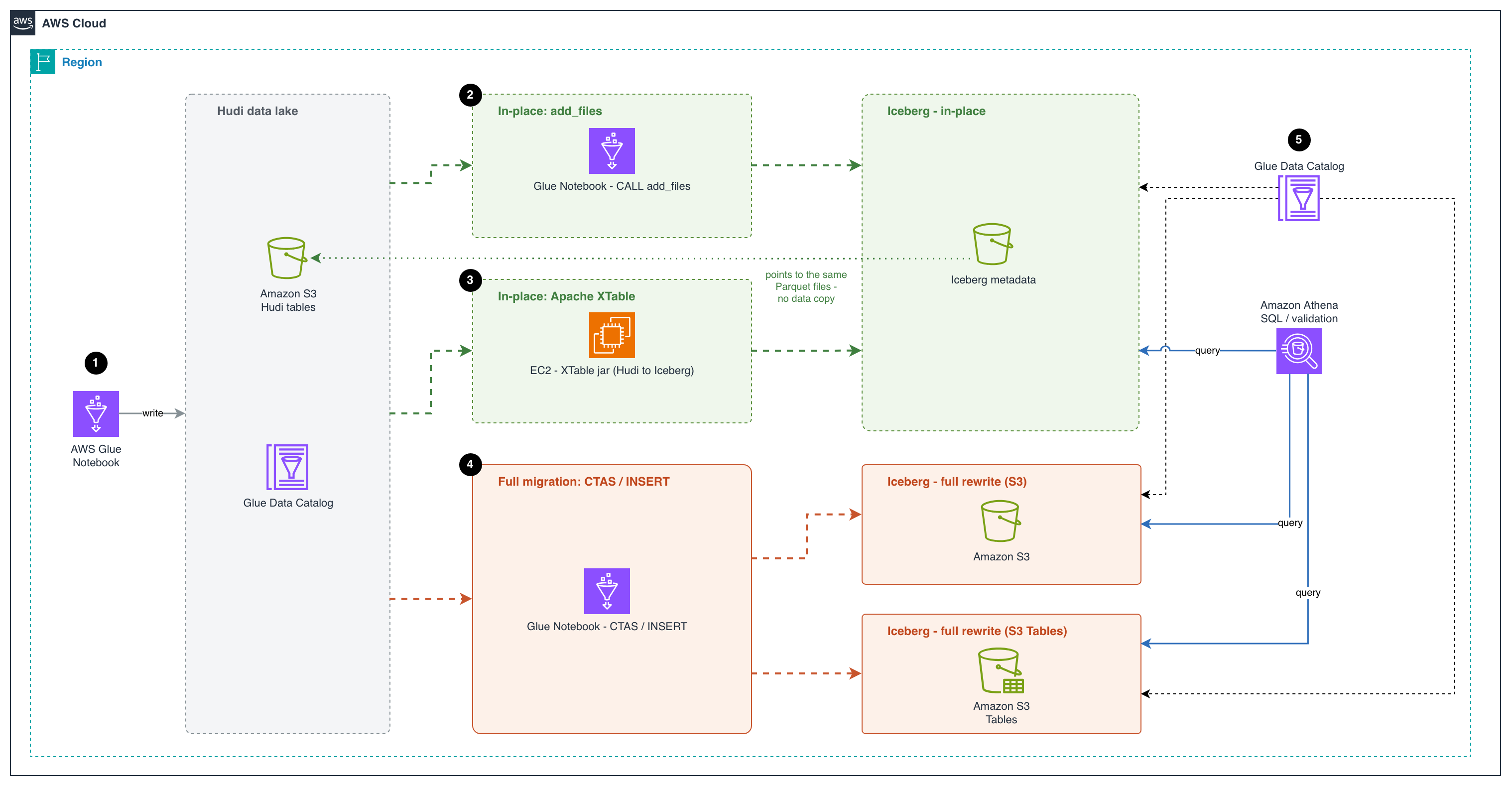
Architecture diagram of the Hudi-to-Iceberg migration workflow on AWS

Figure 1: Migration architecture showing the in-place paths (add_files and Apache XTable) and the full-table paths (CTAS and INSERT) to Amazon S3 and Amazon S3 Tables, all registered in the AWS Glue Data Catalog and queried with Amazon Athena

The workflow consists of the following steps:

An AWS Glue notebook writes the source data as Apache Hudi tables to an Amazon S3 bucket and registers them in the AWS Glue Data Catalog. This creates the existing Hudi data lake that the migration starts from.
The first in-place migration approach uses an AWS Glue notebook to run the Apache Iceberg add_files procedure. The procedure creates Iceberg metadata on top of the Parquet data files already in the Hudi table. The new Iceberg metadata points to the same Parquet files, so no data is copied or rewritten. This makes it a fast, low-cost migration path.
The second in-place migration approach runs Apache XTable on an Amazon Elastic Compute Cloud (Amazon EC2) instance to convert the Hudi table metadata into Iceberg metadata. XTable reads the Hudi commit timeline and creates matching Iceberg metadata that points to the same Parquet files. Both table formats can then share a single copy of the data.
For a full migration, an AWS Glue notebook uses CREATE TABLE AS SELECT (CTAS) or INSERT INTO statements to read the Hudi data and rewrite it as new Iceberg tables. The tables can go in a general purpose S3 bucket or in Amazon S3 Tables. This approach fully separates the new tables from the Hudi source. S3 Tables also handle table maintenance for you, such as compaction and snapshot management.
The AWS Glue Data Catalog registers the Iceberg tables from all three approaches. Users can then use Amazon Athena, a serverless query service, to run SQL queries on these tables and validate the migrated data. Athena enables interactive SQL-based exploration of data directly in Amazon S3 without the need for complex infrastructure management.

Prerequisites

Before getting started, make sure you have the following:

An AWS account with a role that has sufficient access to provision the required resources.
This walkthrough uses AWS Region us-east-1.
An AWS Identity and Access Management (IAM) role for your notebook as described in Set up IAM permissions for AWS Glue Studio and Amazon S3 read and write permission.

Launch an AWS Glue Studio notebook for processing

For this post, we use an AWS Glue Studio notebook. Follow the steps in Getting started with notebooks in AWS Glue Studio to set up the notebook environment.

Sign in to the AWS Management Console and open the AWS Glue console.
In the Region selector (top right), choose your preferred working Region.
Choose ETL Jobs in the left pane.
Choose Notebook under Author using an interactive code notebook, select Start fresh, choose your IAM role, and choose Create notebook.
After a minute, the Jupyter notebook editor appears. Clear all the default cells.

Create Hudi Copy-on-Write (CoW) and Merge-on-Read (MoR) sample event tables

This notebook creates Hudi tables using both Copy-on-Write (CoW) and Merge-on-Read (MoR) table types with sample events. We perform inserts, updates, and deletes, then inspect the underlying file structures to understand the key differences:

CoW: an update or delete fully rewrites every base Parquet file that contains an impacted row, producing a new file slice in the file group. Reads are cheap, and writes amplify with the fraction of files touched.
MoR: an update or delete is appended to an Avro log file alongside the base file instead of rewriting the base, and base + logs are merged at read time (or compacted into a new base file later). Cheaper writes. Costlier reads until compaction.

Execute the first cell with the following configuration to set up the Spark session with Hudi and Iceberg support:

Code:

{
"glue_version": "5.1",
"worker_type": "G.1X",
"number_of_workers": 5,
"idle_timeout": 30,
"--datalake-formats" : "hudi,iceberg",
"--conf" : "spark.serializer=org.apache.spark.serializer.KryoSerializer --conf spark.sql.extensions=org.apache.spark.sql.hudi.HoodieSparkSessionExtension,org.apache.iceberg.spark.extensions.IcebergSparkSessionExtensions --conf spark.sql.catalog.glue_iceberg=org.apache.iceberg.spark.SparkCatalog --conf spark.sql.catalog.glue_iceberg.warehouse=s3://YOUR_BUCKET/warehouse/ --conf spark.sql.catalog.glue_iceberg.type=glue --conf spark.sql.catalog.spark_catalog=org.apache.spark.sql.hudi.catalog.HoodieCatalog --conf spark.kryo.registrator=org.apache.spark.HoodieSparkKryoRegistrar"
}

Initialize the session and configuration. Update the bucket_name, db_name and region variables with your configurations. Reusable helper – list_table_files(table_name, label="", verbose=False) renders a table’s S3 layout as a directory tree so you can SEE how CLEAN, COMPACT and add_files change the files underneath. It is reused before/after each of those steps instead of re-coding the listing.

Code:

# ──────────────────────────────────────────────
# Source Hudi tables
# ──────────────────────────────────────────────
hudi_events_cow_table = "events_hudi_cow" # Copy-on-Write source
hudi_events_mor_table = "events_hudi_mor" # Merge-on-Read source
# ──────────────────────────────────────────────
# In-place migration targets (add_files/xtable)
# ──────────────────────────────────────────────
iceberg_cow_inplace = "events_iceberg_cow_inplace"
iceberg_mor_inplace = "events_iceberg_mor_inplace"
iceberg_cow_xtable = "events_hudi_cow_iceberg_xtable"
iceberg_mor_xtable = "events_hudi_mor_iceberg_xtable"
# ──────────────────────────────────────────────
# Full table (shadow) migration targets
# ──────────────────────────────────────────────
iceberg_cow_full_ctas = "events_iceberg_cow_full_ctas"
iceberg_cow_full_create_insert = "events_iceberg_cow_full_create_insert"
iceberg_mor_full_ctas = "events_iceberg_mor_full_ctas"
iceberg_mor_full_create_insert = "events_iceberg_mor_full_create_insert"
# ──────────────────────────────────────────────
# Infrastructure
# ──────────────────────────────────────────────
bucket_name = "demoblogiceberg-bdb5001" # S3 bucket for data
db_name = "hudi_to_iceberg_blog" # Glue Data Catalog database
region = "us-east-1"
# Create the Glue Data Catalog database
spark.sql(f"""
CREATE DATABASE IF NOT EXISTS {db_name}
LOCATION 's3://{bucket_name}/{db_name}'
""")
# Reusable helper —list_table_files()(S3 layout tree)
import boto3
s3 = boto3.client('s3', region_name=region)
# File/folder annotations keyed by classifier result
_NOTES = {
"hoodie_dir": "<-- Hudi metadata (timeline, schema, indexes)",
"hoodie_mdt": "<-- Hudi metadata table (internal index & stats, MoR)",
"hoodie_files": "<-- file listing index",
"hoodie_cstats":"<-- column-level min/max/null stats",
"hoodie_ridx": "<-- record-key -> file-group mapping",
"ice_meta_dir": "<-- Iceberg metadata layer (metadata.json, manifest lists, manifests)",
"ice_data_dir": "<-- Iceberg data layer (base Parquet files)",
"base": "<-- base Parquet file",
"log": "<-- Hudi delta log file (MoR update, uncompacted)",
"part_meta": "<-- Hudi partition marker",
"metadata_json":"<-- Iceberg table metadata (schema, snapshots)",
"manifest_list":"<-- Iceberg manifest list (snapshot -> manifests)",
"manifest": "<-- Iceberg manifest (lists data files)",
"props": "<-- table configuration & schema",
}
# Fixed-path annotations for metadata directories
_DIR_KIND = {
".hoodie": "hoodie_dir", ".hoodie/metadata": "hoodie_mdt",
".hoodie/metadata/files": "hoodie_files",
".hoodie/metadata/column_stats": "hoodie_cstats",
".hoodie/metadata/record_index": "hoodie_ridx",
"metadata": "ice_meta_dir", "data": "ice_data_dir",
}
def _fmt_size(n):
"""Human-readable byte size."""
for u in ("B", "KB", "MB", "GB", "TB"):
if n < 1024 or u == "TB":
return f"{n:,.0f} {u}" if u == "B" else f"{n:,.1f} {u}"
n /= 1024.0
def _leaf_kind(name):
"""Classify a leaf file by name -> annotation key / count bucket."""
if ".log." in name: return "log"
if name.startswith(".hoodie_partition_metadata"): return "part_meta"
if name == "hoodie.properties": return "props"
if name.endswith(".metadata.json"): return "metadata_json"
if name.startswith("snap-") and name.endswith(".avro"): return "manifest_list"
if name.endswith(".avro"): return "manifest"
if name.endswith(".parquet"): return "base"
return ""
def list_table_files(table_name, label="", verbose=False, max_depth=2, max_children=2):
"""Render a Hudi/Iceberg table's S3 layout as an annotated directory tree.
Teaching view for CLEAN/COMPACT/add_files: multiple base files in a partition
= stale file slices; .log.* = uncompacted MoR updates. The large Hudi .hoodie/
is summarized (depth/width capped); Iceberg metadata/ and data partitions show
in full. verbose=True expands everything.
"""
prefix = f"{db_name}/{table_name}/"
header = f"s3://{bucket_name}/{prefix}"
if label:
header += f" [{label}]"
print(header)
in_meta = lambda p: (p.split("/", 1)[0] if p else "") in (".hoodie", "metadata")
capped_meta = lambda p: (p.split("/", 1)[0] if p else "") == ".hoodie"
# ---- gather objects into a nested tree + tally honest counts -----------
root = {"d": {}, "f": []}
n_base = n_log = n_meta = n_other = 0
s_base = s_log = s_meta = 0
has_hudi = has_ice = False
for page in s3.get_paginator("list_objects_v2").paginate(Bucket=bucket_name, Prefix=prefix):
for obj in page.get("Contents", []):
key = obj["Key"].replace(prefix, "")
size = obj["Size"]
if key == "" or key.endswith("/"):
continue # S3 directory marker
parts = key.split("/")
fname, top = parts[-1], parts[0]
if top == ".hoodie": has_hudi = True
if top == "metadata": has_ice = True
# files inside a metadata folder count ONLY as metadata
if top in (".hoodie", "metadata"):
n_meta += 1; s_meta += size
elif ".log." in fname:
n_log += 1; s_log += size
elif fname.endswith(".parquet"):
n_base += 1; s_base += size
elif fname.startswith(".hoodie"):
n_meta += 1; s_meta += size; has_hudi = True
else:
n_other += 1
node = root
for part in parts[:-1]:
node = node["d"].setdefault(part, {"d": {}, "f": []})
node["f"].append((fname, size))
# ---- helpers -----------------------------------------------------------
def count_all(node):
return len(node["f"]) + sum(count_all(c) for c in node["d"].values())
def collapse(node, name, rel):
"""Merge single-child, file-less dir chains (year=/month=/day=)."""
while (len(node["d"]) == 1 and not node["f"] and not in_meta(rel)):
cname, child = next(iter(node["d"].items()))
crel = f"{rel}/{cname}"
if in_meta(crel): break
name, rel, node = f"{name}/{cname}", crel, child
return name, rel, node
def line(indent, branch, text, note, width):
s = f"{indent}{branch}{text}"
return f"{s:<{width}} {note}" if note else s
def render(node, rel, indent, depth):
entries = ([("d", n, c) for n, c in sorted(node["d"].items())]
+ [("f", n, sz) for n, sz in sorted(node["f"], key=lambda f: (".log." in f[0], f[0]))])
cap = (not verbose) and capped_meta(rel) and len(entries) > max_children
shown = entries[:max_children] if cap else entries
hidden = len(entries) - len(shown)
for i, item in enumerate(shown):
last = (i == len(shown) - 1) and hidden == 0
branch = "└── " if last else "├── "
sub = indent + (" " if last else "│ ")
if item[0] == "d":
_, name, child = item
disp, erel, enode = collapse(child, name, f"{rel}/{name}" if rel else name)
note = _NOTES.get(_DIR_KIND.get(erel, ""), "")
cnt = f" ({count_all(enode)} obj)" if (in_meta(erel) or erel in _DIR_KIND) else ""
print(line(indent, branch, f"{disp}/{cnt}", note, 60))
if (not verbose) and capped_meta(erel) and depth + 1 > max_depth:
inner = count_all(enode)
if inner:
print(f"{sub}└── … ({inner} objects, use verbose=True)")
else:
render(enode, erel, sub, depth + 1)
else:
_, name, size = item
note = _NOTES.get(_leaf_kind(name), "")
print(line(indent, branch, f"{name} ({_fmt_size(size)})", note, 72))
if hidden:
print(f"{indent}└── … (+{hidden} more)")
render(root, "", "", 0)
# ---- per-partition slice note (Hudi concept; skip metadata & Iceberg data/) ----
def slices(node, rel):
top = rel.split("/", 1)[0] if rel else ""
if top in (".hoodie", "metadata", "data"):
return
nb = sum(1 for f, _ in node["f"] if f.endswith(".parquet"))
nl = sum(1 for f, _ in node["f"] if ".log." in f)
if nb > 1:
print(f" note: {rel}/ has {nb} base files -> multiple file slices (stale versions)")
elif nb == 1 and nl:
print(f" note: {rel}/ has 1 base + {nl} log file(s) -> uncompacted MoR updates")
for n, c in node["d"].items():
slices(c, f"{rel}/{n}" if rel else n)
slices(root, "")
# ---- in-place migration note -------------------------------------------
if has_ice and "data" not in root["d"] and n_base == 0:
print(" note: Iceberg metadata/ present but no local data/ folder")
print(" -> in-place migration: data files remain registered in place at the source (Hudi) location; no data copied")
# ---- summary -----------------------------------------------------------
total = n_base + n_log + n_meta + n_other
print(
f"SUMMARY: {n_base} base · {n_log} log · {n_meta} meta"
+ (f" · {n_other} other" if n_other else "")
+ f" · {total} files · {_fmt_size(s_base + s_log + s_meta)}"
)
print(f" .hoodie/: {'present' if has_hudi else 'none'} metadata/ (Iceberg): {'present' if has_ice else 'none'}")
print()

Sample event data

We use a website clickstream events dataset, partitioned by year/month/day – a realistic pattern for event-driven architectures.

Note: In this example, we create the table with a preCombineField, which flips the default write operation of INSERT INTO from insert to upsert. You can override it explicitly with hoodie.spark.sql.insert.into.operation when you need a different behavior.

CoW table: create, upsert, and delete

We create a Hudi CoW table, insert records, apply an upsert, and delete a record, then inspect how the files change.

Create the Hudi CoW events table

Code:

spark.sql(f"""
CREATE TABLE {db_name}.{hudi_events_cow_table} (
event_id STRING,
user_id STRING,
event_type STRING,
event_timestamp TIMESTAMP,
page_url STRING,
year INT,
month INT,
day INT
)
USING HUDI
OPTIONS (
type = 'cow',
primaryKey = 'event_id',
preCombineField = 'event_timestamp'
)
PARTITIONED BY (year, month, day)
LOCATION 's3://{bucket_name}/{db_name}/{hudi_events_cow_table}/'
""")

Insert event records

Code:

spark.sql(f"""
INSERT INTO {db_name}.{hudi_events_cow_table}
VALUES
('EVT_001', 'USER_101', 'page_view', timestamp('2024-04-01 08:15:00'), '/home', 2024, 4, 1),
('EVT_002', 'USER_102', 'click', timestamp('2024-04-01 09:30:00'), '/products', 2024, 4, 1),
('EVT_003', 'USER_103', 'purchase', timestamp('2024-04-02 10:45:00'), '/checkout', 2024, 4, 2),
('EVT_004', 'USER_101', 'page_view', timestamp('2024-04-02 14:20:00'), '/blog', 2024, 4, 2),
('EVT_005', 'USER_104', 'signup', timestamp('2024-04-03 11:00:00'), '/register', 2024, 4, 3),
('EVT_006', 'USER_102', 'click', timestamp('2024-04-03 16:45:00'), '/deals', 2024, 4, 3)
""")

Upsert: simulate late-arriving corrections

Code:

spark.sql(f"""
INSERT INTO {db_name}.{hudi_events_cow_table}
VALUES
('EVT_002', 'USER_102', 'add_to_cart', timestamp('2024-04-01 09:31:00'), '/products/item-42', 2024, 4, 1),
('EVT_005', 'USER_104', 'signup', timestamp('2024-04-03 11:01:00'), '/welcome', 2024, 4, 3)
""")

Delete: remove a record

Code:

spark.sql(f"""
DELETE FROM {db_name}.{hudi_events_cow_table}
WHERE event_id = 'EVT_006'
""")

Inspect the CoW file structure

CoW tables rewrite the entire Parquet file on every upsert/delete. You will see one base Parquet file per file group (no log files).

Code:

list_table_files(hudi_events_cow_table, "COW --- initial file structure")

Output:

s3://demoblogiceberg-bdb5001/hudi_to_iceberg_blog/events_hudi_cow/ [COW — initial file structure]
├── .hoodie/ (50 obj) <-- Hudi metadata (timeline, schema, indexes)
│ ├── .......trimmed
└── year=2024/month=4/
├── day=1/
│ ├── .hoodie_partition_metadata (96 B) <-- Hudi partition marker
│ ├── 7d187e9a.....20261011152509633.parquet (426.3 KB) <-- base Parquet file
│ └── 7d187e9a.....20261011152403779.parquet (426.4 KB) <-- base Parquet file
├── day=2/
│ ├── .hoodie_partition_metadata (96 B) <-- Hudi partition marker
│ └── e583fe17.....20261011152403779.parquet (426.4 KB) <-- base Parquet file
└── day=3/
├── .hoodie_partition_metadata (96 B) <-- Hudi partition marker
├── eedc1b38.....20261011152509633.parquet (426.3 KB) <-- base Parquet file
├── eedc1b38.....20261011152539102.parquet (426.2 KB) <-- base Parquet file
└── eedc1b38.....20261011152403779.parquet (426.4 KB) <-- base Parquet file
note: year=2024/month=4/day=1/ has 2 base files -> multiple file slices (stale versions)
note: year=2024/month=4/day=3/ has 3 base files -> multiple file slices (stale versions)
SUMMARY: 6 base · 0 log · 53 meta · 59 files · 2.8 MB
.hoodie/: present metadata/ (Iceberg): none

MoR table: create, upsert, and delete

We run the same create, upsert, and delete sequence on a Hudi MoR table.

Create the Hudi MoR events table

Code:

spark.sql(f"""
CREATE TABLE {db_name}.{hudi_events_mor_table} (
event_id STRING,
user_id STRING,
event_type STRING,
event_timestamp TIMESTAMP,
page_url STRING,
year INT,
month INT,
day INT
)
USING HUDI
OPTIONS (
type = 'mor',
primaryKey = 'event_id',
preCombineField = 'event_timestamp'
)
PARTITIONED BY (year, month, day)
LOCATION 's3://{bucket_name}/{db_name}/{hudi_events_mor_table}/'
""")

Insert initial event records

Code:

spark.sql(f"""
INSERT INTO {db_name}.{hudi_events_mor_table}
VALUES
('EVT_001', 'USER_201', 'page_view', timestamp('2024-05-10 07:00:00'), '/home', 2024, 5, 10),
('EVT_002', 'USER_202', 'click', timestamp('2024-05-10 08:15:00'), '/products', 2024, 5, 10),
('EVT_003', 'USER_203', 'purchase', timestamp('2024-05-11 09:30:00'), '/checkout', 2024, 5, 11),
('EVT_004', 'USER_201', 'page_view', timestamp('2024-05-11 12:00:00'), '/account', 2024, 5, 11),
('EVT_005', 'USER_204', 'signup', timestamp('2024-05-12 10:30:00'), '/register', 2024, 5, 12),
('EVT_006', 'USER_202', 'click', timestamp('2024-05-12 15:45:00'), '/deals', 2024, 5, 12)
""")

Upsert: simulate late-arriving corrections (creates delta log files)

Code:

spark.sql(f"""
INSERT INTO {db_name}.{hudi_events_mor_table}
VALUES
('EVT_002', 'USER_202', 'add_to_cart', timestamp('2024-05-10 08:16:00'), '/products/item-99', 2024, 5, 10),
('EVT_005', 'USER_204', 'signup', timestamp('2024-05-12 10:31:00'), '/welcome', 2024, 5, 12)
""")

Delete: remove a record

Code:

spark.sql(f"""
DELETE FROM {db_name}.{hudi_events_mor_table}
WHERE event_id = 'EVT_006'
""")

Inspect MoR: base Parquet and log files

MoR tables write updates as delta log files (.log.*) alongside the base Parquet files. This avoids full file rewrites for faster writes.

Code:

list_table_files(hudi_events_mor_table, "MOR --- base parquet + log files")

Output:

s3://demoblogiceberg-bdb5001/hudi_to_iceberg_blog/events_hudi_mor/ [MOR — base parquet + log files]
├── .hoodie/ (50 obj) <-- Hudi metadata (timeline, schema, indexes)
│ ├── .......trimmed
└── year=2024/month=5/
├── day=10/
│ ├── .hoodie_partition_metadata (96 B) <-- Hudi partition marker
│ ├── 7d5ce247.....20261011153110535.parquet (426.4 KB) <-- base Parquet file
│ └── .7d5ce247.....20261011153145862.log.1_1-164-788 (1.3 KB) <-- Hudi delta log file (MoR update, uncompacted)
├── day=11/
│ ├── .hoodie_partition_metadata (96 B) <-- Hudi partition marker
│ └── f9b8147e.....20261011153110535.parquet (426.4 KB) <-- base Parquet file
└── day=12/
├── .hoodie_partition_metadata (96 B) <-- Hudi partition marker
├── 3f0b5ad4.....20261011153110535.parquet (426.4 KB) <-- base Parquet file
├── .3f0b5ad4.....20261011153145862.log.1_0-164-787 (1.3 KB) <-- Hudi delta log file (MoR update, uncompacted)
└── .3f0b5ad4.....20261011153215018.log.1_0-192-901 (1.1 KB) <-- Hudi delta log file (MoR update, uncompacted)
note: year=2024/month=5/day=10/ has 1 base + 1 log file(s) -> uncompacted MoR updates
note: year=2024/month=5/day=12/ has 1 base + 2 log file(s) -> uncompacted MoR updates
SUMMARY: 3 base · 3 log · 53 meta · 59 files · 1.5 MB
.hoodie/: present metadata/ (Iceberg): none

Query both Hudi tables

Code:

print("=== COW Table (events_hudi_cow) ===")
spark.sql(f"SELECT event_id, user_id, event_type, event_timestamp, page_url, year, month, day FROM {db_name}.{hudi_events_cow_table} ORDER BY event_id").show(truncate=False)
print("\n=== MOR Table (events_hudi_mor) ===")
spark.sql(f"SELECT event_id, user_id, event_type, event_timestamp, page_url, year, month, day FROM {db_name}.{hudi_events_mor_table} ORDER BY event_id").show(truncate=False)

Output:

=== COW Table (events_hudi_cow) ===
+--------+--------+-----------+-------------------+-----------------+----+-----+---+
|event_id|user_id |event_type |event_timestamp |page_url |year|month|day|
+--------+--------+-----------+-------------------+-----------------+----+-----+---+
|EVT_001 |USER_101|page_view |2024-04-01 08:15:00|/home |2024|4 |1 |
|EVT_002 |USER_102|add_to_cart|2024-04-01 09:31:00|/products/item-42|2024|4 |1 |
|EVT_003 |USER_103|purchase |2024-04-02 10:45:00|/checkout |2024|4 |2 |
|EVT_004 |USER_101|page_view |2024-04-02 14:20:00|/blog |2024|4 |2 |
|EVT_005 |USER_104|signup |2024-04-03 11:01:00|/welcome |2024|4 |3 |
+--------+--------+-----------+-------------------+-----------------+----+-----+---+
=== MOR Table (events_hudi_mor) ===
+--------+--------+-----------+-------------------+-----------------+----+-----+---+
|event_id|user_id |event_type |event_timestamp |page_url |year|month|day|
+--------+--------+-----------+-------------------+-----------------+----+-----+---+
|EVT_001 |USER_201|page_view |2024-05-10 07:00:00|/home |2024|5 |10 |
|EVT_002 |USER_202|add_to_cart|2024-05-10 08:16:00|/products/item-99|2024|5 |10 |
|EVT_003 |USER_203|purchase |2024-05-11 09:30:00|/checkout |2024|5 |11 |
|EVT_004 |USER_201|page_view |2024-05-11 12:00:00|/account |2024|5 |11 |
|EVT_005 |USER_204|signup |2024-05-12 10:31:00|/welcome |2024|5 |12 |
+--------+--------+-----------+-------------------+-----------------+----+-----+---+

Migrate Hudi tables to Iceberg with in-place migration

In-place migration keeps the original Parquet data files where they are and only builds Iceberg metadata on top of them. There is no rewrite of the underlying data, which makes the migration fast and inexpensive even on large tables. Two tools cover the common cases on AWS:

add_files (Iceberg built-in procedure). A Spark procedure shipped with Apache Iceberg that registers existing Parquet files into an Iceberg table by writing the corresponding manifests, without rewriting the data. It runs as a Spark job in which the source table’s partitions are distributed across Spark tasks, so file listing and column-statistics gathering happen in parallel on the cluster.
Apache XTable (incubating). An open-source cross-format translation tool that can read the metadata of one lakehouse format (Hudi, Delta, or Iceberg) and write out the equivalent metadata for another, pointing at the same underlying Parquet files. XTable can run once to produce the initial Iceberg metadata, or run on a schedule to keep the Iceberg view continuously in sync with ongoing writes to the Hudi table.

Choosing between add_files and Apache XTable for in-place migration

When planning an in-place migration, it is important to understand the strengths of each approach:

add_files is best suited for a one-time migration. It registers existing Hudi Parquet files into an Iceberg table in a single operation. After the migration is complete, the source Hudi table and target Iceberg table are independent, and any subsequent changes to the Hudi table are not reflected in Iceberg.
Apache XTable supports both an initial one-time conversion and ongoing incremental synchronization. This makes it ideal for transition periods where you need to keep both the source Hudi tables and the target Iceberg tables in sync while downstream consumers gradually migrate to Iceberg. After all workloads have been cut over, you can stop the sync process and decommission the Hudi tables.

Important notes

add_files/XTable register existing Parquet files as-is, so they rely on the column names baked into each file. Added and dropped columns are safe, but if the source table was renamed any column during its lifecycle, files written before the rename still hold the old name and reads against the new name return NULL for them. For tables with a history of column renames, prefer a full migration instead.

Iceberg version and column statistics (in-place add_files / snapshot): In Iceberg 1.9.0 through 1.10.0, the add_files and snapshot procedures don’t generate column stats in the Iceberg metadata. The cause is a NameMapping loss in ParquetUtil.footerMetrics. Without those column-level lower/upper bounds and null counts, the migrated Iceberg table loses most of its file-skipping ability at query planning time, which translates into more Parquet files being inspected, higher scan volume, and slower queries, especially for selective filters on non-partition columns. The issue is fixed in the Iceberg 1.10.1 release (#14617). Affected runtimes are AWS Glue 5.1 and Amazon EMR 7.11–7.13. We recommend AWS Glue 6.0+ or Amazon EMR 7.14+ for production migrations.

Shared data files during in-place migration: With both approaches, the in-place migration doesn’t copy data. The resulting Iceberg table points to the same underlying Parquet files as the source Hudi table. This means that until you perform a full cutover to Iceberg, you must avoid destructive operations on the Iceberg table that could delete or modify the shared data files. Specifically:

Don’t drop the Iceberg table with the PURGE option.
Don’t run Iceberg maintenance tasks such as expire_snapshots or remove_orphan_files.

Running any of these before cutover can remove files that the source Hudi table still depends on, leading to data loss. Iceberg exposes a built-in guardrail against this: the gc.enabled table property. When set to false, Iceberg blocks the preceding destructive operations. How you apply this depends on which migration path you choose.

With add_files. Disable garbage collection immediately after the procedure finishes and keep it disabled until you have fully cut over to Iceberg.

Right after add_files:

spark.sql(f"""
ALTER TABLE {db_name}.{table_name}
SET TBLPROPERTIES ('gc.enabled' = 'false');
""")

After Hudi source is retired and the Iceberg table owns its own data, re-enable GC so maintenance can run normally:

spark.sql(f"""
ALTER TABLE {db_name}.{table_name}
SET TBLPROPERTIES ('gc.enabled' = 'true');
""")

With Apache XTable (incremental sync). The gc.enabled = false guardrail is only partially usable here, because XTable’s incremental sync needs GC to be enabled on the Iceberg table to operate normally. A practical pattern is:

Run the initial full XTable sync.
Temporarily set gc.enabled = false to run post-migration validation and consistency checks on the Iceberg table in a safe state.
Set gc.enabled = true again before starting incremental sync and leave it on for the duration of the sync period.

Because the automatic guardrail is off during incremental sync, the burden shifts to operational discipline: as long as XTable is syncing and data files are shared with the Hudi table, don’t run any Iceberg operation that can delete source data files (no DROP TABLE ... PURGE, no expire_snapshots, no remove_orphan_files, no manual object deletion against the shared S3 prefix). Treat the Iceberg table as read-only in terms of file lifecycle until cutover is complete, and Hudi is decommissioned, at which point normal Iceberg maintenance can resume.

Don’t enable the AWS Glue Data Catalog table optimizer before cutover.

Glue-managed Iceberg maintenance (compaction, snapshot retention, orphan file cleanup) will rewrite or delete the Parquet files that the source Hudi table still depends on. Verify that no catalog-level optimizer applies to the migrated table and leave table-level optimization off until cutover is complete.

Prerequisites for in-place migration with add_files. The add_files procedure registers every Parquet file it finds under the source location into the target Iceberg table, with no awareness of Hudi’s file-group versioning. If more than one file version of the same record is present at migration time, each version is registered as a separate row, and the Iceberg table will contain duplicates. The source Hudi table must therefore expose exactly one file version per record before add_files runs:

CoW tables: Run CLEAN to remove old file versions, keeping only the latest Parquet files.
MoR tables: Run COMPACTION (merge delta logs into base Parquet) + CLEAN before calling add_files, since add_files can only register base Parquet files and cannot process Hudi delta log files.

Option 1: Migrate Hudi tables to Iceberg with the add_files Spark procedure

This option uses the Iceberg add_files procedure to register the existing Hudi Parquet files into new Iceberg tables. Run it once per table, after preparing the Hudi table so that only the current file versions remain.

Migrate CoW to Iceberg

We create the target Iceberg table, prepare the Hudi source so that only the current file versions remain, register those files, and validate the result.

Create the target Iceberg table with the same schema

Code:

spark.sql(f"""
CREATE TABLE glue_iceberg.{db_name}.{iceberg_cow_inplace} (
event_id STRING,
user_id STRING,
event_type STRING,
event_timestamp TIMESTAMP,
page_url STRING,
year INT,
month INT,
day INT
)
USING iceberg
PARTITIONED BY (year, month, day)
LOCATION 's3://{bucket_name}/{db_name}/{iceberg_cow_inplace}/'
""")

Run Hudi CLEAN to keep only the latest file versions

Check files listing for the Hudi table before the CLEAN operation:

Code:

list_table_files(hudi_events_cow_table, "COW --- BEFORE CLEAN")

Output:

s3://demoblogiceberg-bdb5001/hudi_to_iceberg_blog/events_hudi_cow/ [COW — BEFORE CLEAN]
├── .hoodie/ (50 obj) <-- Hudi metadata (timeline, schema, indexes)
│ ├── .......trimmed
└── year=2024/month=4/
├── day=1/
│ ├── .hoodie_partition_metadata (96 B) <-- Hudi partition marker
│ ├── 7d187e9a.....20261011152509633.parquet (426.3 KB) <-- base Parquet file
│ └── 7d187e9a.....20261011152403779.parquet (426.4 KB) <-- base Parquet file
├── day=2/
│ ├── .hoodie_partition_metadata (96 B) <-- Hudi partition marker
│ └── e583fe17.....20261011152403779.parquet (426.4 KB) <-- base Parquet file
└── day=3/
├── .hoodie_partition_metadata (96 B) <-- Hudi partition marker
├── eedc1b38.....20261011152509633.parquet (426.3 KB) <-- base Parquet file
├── eedc1b38.....20261011152539102.parquet (426.2 KB) <-- base Parquet file
└── eedc1b38.....20261011152403779.parquet (426.4 KB) <-- base Parquet file
note: year=2024/month=4/day=1/ has 2 base files -> multiple file slices (stale versions)
note: year=2024/month=4/day=3/ has 3 base files -> multiple file slices (stale versions)
SUMMARY: 6 base · 0 log · 53 meta · 59 files · 2.8 MB
.hoodie/: present metadata/ (Iceberg): none

Run the CLEAN operation specifying to keep only the latest file slices:

Code:

spark.sql(f"""
CALL spark_catalog.system.run_clean(
table => '{db_name}.{hudi_events_cow_table}',
clean_policy => 'KEEP_LATEST_FILE_VERSIONS',
file_versions_retained => 1
)
""").show(truncate=False)

Output:

+-----------------+--------------------+-------------------+-------------------------+-----------------------+-------+
|start_clean_time |time_taken_in_millis|total_files_deleted|earliest_commit_to_retain|bootstrap_part_metadata|version|
+-----------------+--------------------+-------------------+-------------------------+-----------------------+-------+
|20261011154407413|382 |3 | |{} |2 |
+-----------------+--------------------+-------------------+-------------------------+-----------------------+-------+

Check files listing for the Hudi table after the CLEAN operation:

Code:

list_table_files(hudi_events_cow_table, "COW --- AFTER CLEAN")

Output:

s3://demoblogiceberg-bdb5001/hudi_to_iceberg_blog/events_hudi_cow/ [COW — AFTER CLEAN]
├── .hoodie/ (59 obj) <-- Hudi metadata (timeline, schema, indexes)
│ ├── .......trimmed
└── year=2024/month=4/
├── day=1/
│ ├── .hoodie_partition_metadata (96 B) <-- Hudi partition marker
│ └── 7d187e9a.....20261011152509633.parquet (426.3 KB) <-- base Parquet file
├── day=2/
│ ├── .hoodie_partition_metadata (96 B) <-- Hudi partition marker
│ └── e583fe17.....20261011152403779.parquet (426.4 KB) <-- base Parquet file
└── day=3/
├── .hoodie_partition_metadata (96 B) <-- Hudi partition marker
└── eedc1b38.....20261011152539102.parquet (426.2 KB) <-- base Parquet file
SUMMARY: 3 base · 0 log · 62 meta · 65 files · 1.6 MB
.hoodie/: present metadata/ (Iceberg): none

Register Hudi Parquet files into Iceberg with add_files

Code:

spark.sql(f"""
CALL glue_iceberg.system.add_files(
source_table => 'parquet.`s3://{bucket_name}/{db_name}/{hudi_events_cow_table}/`',
table => 'glue_iceberg.{db_name}.{iceberg_cow_inplace}'
)
""").show(truncate=False)

Output:

+-----------------+-----------------------+
|added_files_count|changed_partition_count|
+-----------------+-----------------------+
|3 |NULL |
+-----------------+-----------------------+

Validate: compare Hudi CoW and Iceberg (in-place)

We can see the Hudi and Iceberg tables reflect the same content:

Code:

print("Source: Hudi COW")
spark.sql(f"SELECT event_id, user_id, event_type, event_timestamp, page_url FROM {db_name}.{hudi_events_cow_table} ORDER BY event_id").show(truncate=False)
print("Target: Iceberg (in-place)")
spark.sql(f"SELECT event_id, user_id, event_type, event_timestamp, page_url FROM glue_iceberg.{db_name}.{iceberg_cow_inplace} ORDER BY event_id").show(truncate=False)

Output:

Source: Hudi COW
+--------+--------+-----------+-------------------+-----------------+
|event_id|user_id |event_type |event_timestamp |page_url |
+--------+--------+-----------+-------------------+-----------------+
|EVT_001 |USER_101|page_view |2024-04-01 08:15:00|/home |
|EVT_002 |USER_102|add_to_cart|2024-04-01 09:31:00|/products/item-42|
|EVT_003 |USER_103|purchase |2024-04-02 10:45:00|/checkout |
|EVT_004 |USER_101|page_view |2024-04-02 14:20:00|/blog |
|EVT_005 |USER_104|signup |2024-04-03 11:01:00|/welcome |
+--------+--------+-----------+-------------------+-----------------+
Target: Iceberg (in-place)
+--------+--------+-----------+-------------------+-----------------+
|event_id|user_id |event_type |event_timestamp |page_url |
+--------+--------+-----------+-------------------+-----------------+
|EVT_001 |USER_101|page_view |2024-04-01 08:15:00|/home |
|EVT_002 |USER_102|add_to_cart|2024-04-01 09:31:00|/products/item-42|
|EVT_003 |USER_103|purchase |2024-04-02 10:45:00|/checkout |
|EVT_004 |USER_101|page_view |2024-04-02 14:20:00|/blog |
|EVT_005 |USER_104|signup |2024-04-03 11:01:00|/welcome |
+--------+--------+-----------+-------------------+-----------------+

We can see under the Iceberg table location only Iceberg metadata has been generated. These point to the source Hudi table data files.

Code:

list_table_files(iceberg_cow_inplace, "COW Iceberg --- AFTER add_files (note metadata/ folder)", verbose=True)

Output:

s3://demoblogiceberg-bdb5001/hudi_to_iceberg_blog/events_iceberg_cow_inplace/ [COW Iceberg — AFTER add_files (note metadata/ folder)]
└── metadata/ (5 obj) <-- Iceberg metadata layer (metadata.json, manifest lists, manifests)
├── 00000.....metadata.json (1.3 KB) <-- Iceberg table metadata (schema, snapshots)
├── 00001.....metadata.json (2.0 KB) <-- Iceberg table metadata (schema, snapshots)
├── 00002.....metadata.json (3.0 KB) <-- Iceberg table metadata (schema, snapshots)
├── snap-7577.....avro (4.4 KB) <-- Iceberg manifest list (snapshot -> manifests)
└── stage-223...-manifest.....avro (6.7 KB) <-- Iceberg manifest (lists data files)
note: Iceberg metadata/ present but no local data/ folder
-> in-place migration: data files remain registered in place at the source (Hudi) location; no data copied
SUMMARY: 0 base · 0 log · 5 meta · 5 files · 17.4 KB
.hoodie/: none metadata/ (Iceberg): present

Migrate MoR to Iceberg

For the MoR table, we compact and clean the Hudi source first, then register the compacted files and validate the result.

Create the target Iceberg table

Code:

spark.sql(f"""
CREATE TABLE glue_iceberg.{db_name}.{iceberg_mor_inplace} (
event_id STRING,
user_id STRING,
event_type STRING,
event_timestamp TIMESTAMP,
page_url STRING,
year INT,
month INT,
day INT
)
USING iceberg
PARTITIONED BY (year, month, day)
LOCATION 's3://{bucket_name}/{db_name}/{iceberg_mor_inplace}/'
""")

Compact the MoR table: merge delta logs into base Parquet files

Check files listing for the Hudi table before the CLEAN operation:

Code:

list_table_files(hudi_events_mor_table, "MOR --- BEFORE COMPACT+CLEAN")

Output:

s3://demoblogiceberg-bdb5001/hudi_to_iceberg_blog/events_hudi_mor/ [MOR — BEFORE COMPACT+CLEAN]
├── .hoodie/ (50 obj) <-- Hudi metadata (timeline, schema, indexes)
│ ├── .......trimmed
└── year=2024/month=5/
├── day=10/
│ ├── .hoodie_partition_metadata (96 B) <-- Hudi partition marker
│ ├── 7d5ce247.....20261011153110535.parquet (426.4 KB) <-- base Parquet file
│ └── .7d5ce247.....20261011153145862.log.1_1-164-788 (1.3 KB) <-- Hudi delta log file (MoR update, uncompacted)
├── day=11/
│ ├── .hoodie_partition_metadata (96 B) <-- Hudi partition marker
│ └── f9b8147e.....20261011153110535.parquet (426.4 KB) <-- base Parquet file
└── day=12/
├── .hoodie_partition_metadata (96 B) <-- Hudi partition marker
├── 3f0b5ad4.....20261011153110535.parquet (426.4 KB) <-- base Parquet file
├── .3f0b5ad4.....20261011153145862.log.1_0-164-787 (1.3 KB)
└── .3f0b5ad4.....20261011153215018.log.1_0-192-901 (1.1 KB) <-- Hudi delta log file (MoR update, uncompacted)
note: year=2024/month=5/day=10/ has 1 base + 1 log file(s) -> uncompacted MoR updates
note: year=2024/month=5/day=12/ has 1 base + 2 log file(s) -> uncompacted MoR updates
SUMMARY: 3 base · 3 log · 53 meta · 59 files · 1.5 MB
.hoodie/: present metadata/ (Iceberg): none

Trigger COMPACTION scheduling on the MoR table with the delta-commit and age thresholds set to their minimum, so any file slice with pending log files is included in the plan and merged back into its base Parquet file.

Code:

# Schedule compaction
spark.sql(f"""
CALL spark_catalog.system.run_compaction(
table => '{db_name}.{hudi_events_mor_table}',
op => 'schedule',
options =>
'hoodie.compact.inline.max.delta.commits=1,
hoodie.compact.inline.max.delta.seconds=0'
)
""").show(truncate=False)

Output:

+-----------------+--------------+---------+
|timestamp |operation_size|state |
+-----------------+--------------+---------+
|20261011154522819|2 |REQUESTED|
+-----------------+--------------+---------+

Execute the previously scheduled compaction plan to merge the pending log files into their base Parquet files. The REQUESTED instant produced by the schedule step transitions to COMPLETED, and the table is left with base Parquet files only.

Code:

# Execute compaction
spark.sql(f"""
CALL spark_catalog.system.run_compaction(
table => '{db_name}.{hudi_events_mor_table}',
op => 'run'
)
""").show(truncate=False)

Output:

+-----------------+--------------+---------+
|timestamp |operation_size|state |
+-----------------+--------------+---------+
|20261011154522819|2 |COMPLETED|
+-----------------+--------------+---------+

Run Hudi CLEAN to remove old file versions and log files

Code:

spark.sql(f"""
CALL spark_catalog.system.run_clean(
table => '{db_name}.{hudi_events_mor_table}',
clean_policy => 'KEEP_LATEST_FILE_VERSIONS',
file_versions_retained => 1
)
""").show(truncate=False)

Output:

+-----------------+--------------------+-------------------+-------------------------+-----------------------+-------+
|start_clean_time |time_taken_in_millis|total_files_deleted|earliest_commit_to_retain|bootstrap_part_metadata|version|
+-----------------+--------------------+-------------------+-------------------------+-----------------------+-------+
|20261011154552026|345 |5 | |{} |2 |
+-----------------+--------------------+-------------------+-------------------------+-----------------------+-------+

Code:

list_table_files(hudi_events_mor_table, "MOR --- AFTER COMPACT+CLEAN")

Output:

s3://demoblogiceberg-bdb5001/hudi_to_iceberg_blog/events_hudi_mor/ [MOR — AFTER COMPACT+CLEAN]
├── .hoodie/ (69 obj) <-- Hudi metadata (timeline, schema, indexes)
│ ├── .......trimmed
└── year=2024/month=5/
├── day=10/
│ ├── .hoodie_partition_metadata (96 B) <-- Hudi partition marker
│ └── 7d5ce247.....20261011154522819.parquet (426.3 KB) <-- base Parquet file
├── day=11/
│ ├── .hoodie_partition_metadata (96 B) <-- Hudi partition marker
│ └── f9b8147e.....20261011153110535.parquet (426.4 KB) <-- base Parquet file
└── day=12/
├── .hoodie_partition_metadata (96 B) <-- Hudi partition marker
└── 3f0b5ad4.....20261011154522819.parquet (426.1 KB) <-- base Parquet file
SUMMARY: 3 base · 0 log · 72 meta · 75 files · 1.7 MB
.hoodie/: present metadata/ (Iceberg): none

Register compacted Parquet files into Iceberg with add_files

Code:

spark.sql(f"""
CALL glue_iceberg.system.add_files(
source_table => 'parquet.`s3://{bucket_name}/{db_name}/{hudi_events_mor_table}/`',
table => 'glue_iceberg.{db_name}.{iceberg_mor_inplace}'
)
""").show(truncate=False)

Output:

+-----------------+-----------------------+
|added_files_count|changed_partition_count|
+-----------------+-----------------------+
|3 |NULL |
+-----------------+-----------------------+

Refresh the Hudi table to invalidate Spark’s cached metadata and file listings, so subsequent queries re-read the post-compaction state from the catalog and storage instead of returning stale pre-compaction results.

Code:

spark.sql(f"REFRESH TABLE {db_name}.{hudi_events_mor_table}")

Validate: compare Hudi MoR and Iceberg (in-place)

Code:

print("Source: Hudi MOR")
spark.sql(f"SELECT event_id, user_id, event_type, event_timestamp, page_url FROM {db_name}.{hudi_events_mor_table} ORDER BY event_id").show(truncate=False)
print("Target: Iceberg (in-place)")
spark.sql(f"SELECT event_id, user_id, event_type, event_timestamp, page_url FROM glue_iceberg.{db_name}.{iceberg_mor_inplace} ORDER BY event_id").show(truncate=False)

Output:

Source: Hudi MOR
+--------+--------+-----------+-------------------+-----------------+
|event_id|user_id |event_type |event_timestamp |page_url |
+--------+--------+-----------+-------------------+-----------------+
|EVT_001 |USER_201|page_view |2024-05-10 07:00:00|/home |
|EVT_002 |USER_202|add_to_cart|2024-05-10 08:16:00|/products/item-99|
|EVT_003 |USER_203|purchase |2024-05-11 09:30:00|/checkout |
|EVT_004 |USER_201|page_view |2024-05-11 12:00:00|/account |
|EVT_005 |USER_204|signup |2024-05-12 10:31:00|/welcome |
+--------+--------+-----------+-------------------+-----------------+
Target: Iceberg (in-place)
+--------+--------+-----------+-------------------+-----------------+
|event_id|user_id |event_type |event_timestamp |page_url |
+--------+--------+-----------+-------------------+-----------------+
|EVT_001 |USER_201|page_view |2024-05-10 07:00:00|/home |
|EVT_002 |USER_202|add_to_cart|2024-05-10 08:16:00|/products/item-99|
|EVT_003 |USER_203|purchase |2024-05-11 09:30:00|/checkout |
|EVT_004 |USER_201|page_view |2024-05-11 12:00:00|/account |
|EVT_005 |USER_204|signup |2024-05-12 10:31:00|/welcome |
+--------+--------+-----------+-------------------+-----------------+

Code:

list_table_files(iceberg_mor_inplace, "MOR Iceberg --- AFTER add_files (note metadata/ folder)", verbose=True)

Output:

s3://demoblogiceberg-bdb5001/hudi_to_iceberg_blog/events_iceberg_mor_inplace/ [MOR Iceberg — AFTER add_files (note metadata/ folder)]
└── metadata/ (5 obj) <-- Iceberg metadata layer (metadata.json, manifest lists, manifests)
├── 00000.....metadata.json (1.3 KB) <-- Iceberg table metadata (schema, snapshots)
├── 00001.....metadata.json (2.0 KB) <-- Iceberg table metadata (schema, snapshots)
├── 00002.....metadata.json (3.0 KB) <-- Iceberg table metadata (schema, snapshots)
├── snap-5097.....avro (4.4 KB) <-- Iceberg manifest list (snapshot -> manifests)
└── stage-254...-manifest.....avro (6.7 KB) <-- Iceberg manifest (lists data files)
note: Iceberg metadata/ present but no local data/ folder
-> in-place migration: data files remain registered in place at the source (Hudi) location; no data copied
SUMMARY: 0 base · 0 log · 5 meta · 5 files · 17.4 KB
.hoodie/: none metadata/ (Iceberg): present

Option 2: Migrate Hudi tables to Iceberg with the Apache XTable sync tool

Apache XTable (Incubating) is an open-source interoperability layer that translates metadata between Apache Hudi, Apache Iceberg, and Delta Lake without copying data. Its sync utility supports both one-time conversion and ongoing incremental synchronization, enabling parallel access to source and target formats during migration. Because it ships as a self-contained Java process with no managed-service dependency, you can run it anywhere a JVM is available: a developer laptop for one-off conversions, an Amazon Elastic Container Service (Amazon ECS) or Amazon Elastic Kubernetes Service (Amazon EKS) container, or an AWS Lambda function, triggered on a schedule through Amazon EventBridge or on an event such as a new Hudi commit.

XTable’s sync utility does two things:

First run – performs the initial in-place migration of a Hudi table to Iceberg.
Subsequent runs – keep the Iceberg metadata in sync with the source table as it continues to receive writes.

Compile xtable-utilities following the instructions in the Apache XTable GitHub repository and copy xtable-utilities/target/xtable-utilities_2.12-0.5.0-SNAPSHOT-bundled.jar into the current working directory.

Migrate MoR to Iceberg

Note: When running the XTable sync tool on a MoR table, the utility only reads the base Parquet files and doesn’t process the delta log files. As a result, the generated Iceberg metadata reflects only the Hudi read-optimized view, meaning any recent updates or deletes stored in delta logs will be missing. To avoid data loss, always run compaction on the MoR table before executing the sync tool (for example, similar run_compaction commands as for the add_files example). Unlike add_files, however, there is no need to run CLEAN beforehand: XTable doesn’t scan the table location file by file, but builds the Iceberg manifests from Hudi’s own metadata, so it already knows which Parquet files belong to the current file slices and ignores superseded versions automatically.

Configure Apache XTables Configuration files.

Create the datasetConfig.yaml file containing indications about the dataset(s) to convert with the following content:

sourceFormat: HUDI
targetFormats:
  - ICEBERG
datasets:
  - tableBasePath: s3://YOUR_BUCKET/hudi_to_iceberg_blog/events_hudi_mor/
    tableName: events_hudi_mor_iceberg_xtable
    namespace: hudi_to_iceberg_blog
    partitionSpec: year:VALUE,month:VALUE,day:VALUE

Create the glueDataCatalog.yaml file containing Iceberg catalog (AWS Glue Data Catalog) settings with the following content:

catalogImpl: org.apache.iceberg.aws.glue.GlueCatalog
catalogName: glue
catalogOptions:
  warehouse: s3://YOUR_BUCKET/warehouse/
  catalog-impl: org.apache.iceberg.aws.glue.GlueCatalog
  io-impl: org.apache.iceberg.aws.s3.S3FileIO

Run the conversion

export AWS_DEFAULT_REGION=us-east-1

java -jar incubator-xtable/xtable-utilities/target/xtable-utilities_2.12-0.5.0-SNAPSHOT-bundled.jar \
-d datasetConfig.yaml \
-i glueDataCatalog.yaml

CLI options (from --help)

Flag	Long form	Description
`-d`	`--datasetConfig`	Path to the dataset configuration YAML (required)
`-i`	`--icebergCatalogConfig`	Path to the Iceberg catalog config YAML
`-c`	`--convertersConfig`	Override converter configs
`-p`	`--hadoopConfig`	Extra Hadoop config XML
`-m`	`--continuousMode`	Run on a scheduled loop
`-t`	`--continuousModeInterval`	Loop interval in seconds (with `-m`)

Verify the result

% aws glue get-table --database-name hudi_to_iceberg_blog \
--name events_hudi_mor_iceberg_xtable \
--query 'Table.{Name:Name,Type:Parameters.table_type,MetaLoc:Parameters.metadata_location}'

{
  "Name": "events_hudi_mor_iceberg_xtable",
  "Type": "ICEBERG",
  "MetaLoc": "s3://YOUR_BUCKET/hudi_to_iceberg_blog/events_hudi_mor/metadata/00002-a88318ba-ad13-4a0c-85a8-d595b53e9a89.metadata.json"
}

% aws s3 ls s3://YOUR_BUCKET/hudi_to_iceberg_blog/events_hudi_mor/metadata/
2026-09-22 16:26:18        648 00000-c71bcac6-3eee-4b98-875f-7562770db80b.metadata.json
2026-09-22 16:26:19       1940 00001-941c5622-95e3-41d7-942a-dabd69e561d1.metadata.json
2026-09-22 16:26:20       4293 00002-a88318ba-ad13-4a0c-85a8-d595b53e9a89.metadata.json
2026-09-22 16:26:20       8845 11adf6a4-58b9-4cc2-8cf0-317a7b43a8f7-m0.avro
2026-09-22 16:26:20       4493 snap-8409429281635613515-1-11adf6a4-58b9-4cc2-8cf0-317a7b43a8f7.avro

Amazon Athena console query returning five rows from the migrated Iceberg table

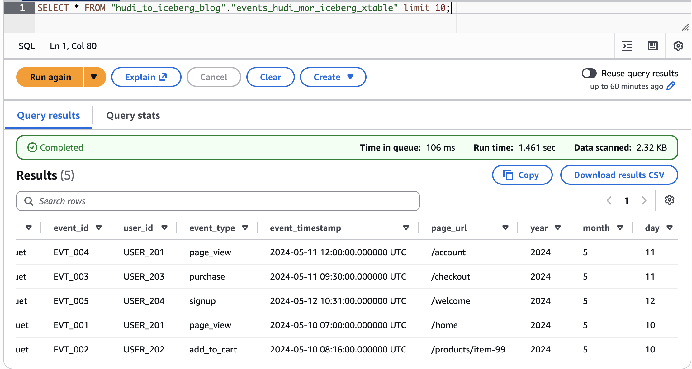
Figure 2: Validating the Apache XTable conversion by querying the migrated Iceberg table in Amazon Athena

Note: If you keep ingesting into the source Hudi table and want to keep the Iceberg table in sync, re-run the same conversion command. XTable automatically detects the previous execution and runs in incremental mode.

Migrate CoW to Iceberg

For the CoW table, update the datasetConfig.yaml with the CoW table path and name.

sourceFormat: HUDI
targetFormats:
  - ICEBERG
datasets:
  - tableBasePath: s3://YOUR_BUCKET/hudi_to_iceberg_blog/events_hudi_cow/
    tableName: events_hudi_mor_iceberg_xtable
    namespace: hudi_to_iceberg_blog
    partitionSpec: year:VALUE,month:VALUE,day:VALUE

The glueDataCatalog.yaml, conversion command, and verification steps remain the same as described in the MOR example.

Migrate Hudi tables to Iceberg with full table migration

Full table migration (also called shadow migration) reads all data from Hudi and writes it into a brand-new Iceberg table. This approach:

Allows schema and partition evolution (for example, switching to Iceberg hidden partitioning).
Produces a clean Iceberg table with no Hudi metadata dependencies.
Requires additional storage (data is copied)

Two options are demonstrated:

Option A: CTAS – a single-statement CREATE TABLE ... AS SELECT.
Option B: CREATE + INSERT – explicit table creation followed by data insertion.

Note: When performing a full table migration, the process is the same regardless of whether your source is a Hudi CoW or MoR table. This is because Spark reads from the Hudi real-time view by default, which reflects the latest table state. For CoW tables, this means reading the current base Parquet files. For MoR tables, the real-time view automatically merges the base Parquet files with any pending delta log files, ensuring all recent inserts, updates, and deletes are captured. As a result, the migrated Iceberg table will contain a complete and up-to-date snapshot of your data, with no additional compaction or cleanup steps required before migration.

We have taken a Hudi CoW table example to demonstrate the migration from Hudi CoW table to Iceberg table.

Prepare the column list for migration

Filter out Hudi internal metadata columns (_hoodie_*) and explicit partition columns to use Iceberg hidden partitioning.

Code:

# Build column list excluding Hudi metadata and explicit partition columns
all_columns_cow = spark.sql(f"SELECT * FROM {db_name}.{hudi_events_cow_table} LIMIT 1").columns
non_hoodie_columns_cow = [col for col in all_columns_cow if not col.startswith("_hoodie")]
partition_cols = ['year', 'month', 'day']
data_columns_cow = [col for col in non_hoodie_columns_cow if col not in partition_cols]
columns_to_select_cow = ", ".join(data_columns_cow)
print(f"Columns for COW migration: {columns_to_select_cow}")

Output:

Columns for COW migration: event_id, user_id, event_type, event_timestamp, page_url

Migrate CoW to Iceberg (full table / shadow migration)

We show two full-migration options: a single-statement CTAS and an explicit CREATE followed by INSERT.

Option A: CTAS (CREATE TABLE AS SELECT)

Single statement that creates the Iceberg table and populates it in one step. Here we also adopt Iceberg hidden partitioning by days(event_timestamp) – no need for explicit year/month/day columns.

Code:

spark.sql(f"""
CREATE TABLE glue_iceberg.{db_name}.{iceberg_cow_full_ctas}
USING ICEBERG
PARTITIONED BY (days(event_timestamp))
LOCATION 's3://{bucket_name}/{db_name}/{iceberg_cow_full_ctas}/'
AS (SELECT {columns_to_select_cow} FROM {db_name}.{hudi_events_cow_table})
""")

Code:

# Verify CTAS migration
print("Iceberg COW (CTAS) - Full Migration")
spark.sql(f"SELECT * FROM glue_iceberg.{db_name}.{iceberg_cow_full_ctas} ORDER BY event_id").show(truncate=False)

Output:

Iceberg COW (CTAS) - Full Migration
+--------+--------+-----------+-------------------+-----------------+
|event_id|user_id |event_type |event_timestamp |page_url |
+--------+--------+-----------+-------------------+-----------------+
|EVT_001 |USER_101|page_view |2024-04-01 08:15:00|/home |
|EVT_002 |USER_102|add_to_cart|2024-04-01 09:31:00|/products/item-42|
|EVT_003 |USER_103|purchase |2024-04-02 10:45:00|/checkout |
|EVT_004 |USER_101|page_view |2024-04-02 14:20:00|/blog |
|EVT_005 |USER_104|signup |2024-04-03 11:01:00|/welcome |
+--------+--------+-----------+-------------------+-----------------+

Option B: CREATE + INSERT

Useful when you need more control over the target table schema or want to add table properties before loading data, such as sort order. It is also a good fit for very large source tables, because the load phase is a plain INSERT INTO that you can run partition by partition, giving you control over parallelism, resource usage, and resumability during the migration.

Code:

spark.sql(f"""
CREATE TABLE glue_iceberg.{db_name}.{iceberg_cow_full_create_insert} (
event_id STRING,
user_id STRING,
event_type STRING,
event_timestamp TIMESTAMP,
page_url STRING
)
USING iceberg
PARTITIONED BY (days(event_timestamp))
LOCATION 's3://{bucket_name}/{db_name}/{iceberg_cow_full_create_insert}/'
""")

Code:

spark.sql(f"""
INSERT INTO glue_iceberg.{db_name}.{iceberg_cow_full_create_insert}
SELECT {columns_to_select_cow}
FROM {db_name}.{hudi_events_cow_table}
""")

Code:

# Verify CREATE + INSERT migration
print("Iceberg COW (CREATE+INSERT) - Full Migration")
spark.sql(f"SELECT * FROM glue_iceberg.{db_name}.{iceberg_cow_full_create_insert} ORDER BY event_id").show(truncate=False)

Output:

Iceberg COW (CREATE+INSERT) - Full Migration
+--------+--------+-----------+-------------------+-----------------+
|event_id|user_id |event_type |event_timestamp |page_url |
+--------+--------+-----------+-------------------+-----------------+
|EVT_001 |USER_101|page_view |2024-04-01 08:15:00|/home |
|EVT_002 |USER_102|add_to_cart|2024-04-01 09:31:00|/products/item-42|
|EVT_003 |USER_103|purchase |2024-04-02 10:45:00|/checkout |
|EVT_004 |USER_101|page_view |2024-04-02 14:20:00|/blog |
|EVT_005 |USER_104|signup |2024-04-03 11:01:00|/welcome |
+--------+--------+-----------+-------------------+-----------------+

Full table migration of Hudi to Amazon S3 Tables

Create a new notebook following the same procedure described earlier, updating the configuration as shown in the following steps.

Configure the Spark session

Change <ACCOUNT_ID>, <REGION>, and <TABLE_BUCKET_NAME> to your S3 Tables bucket details.

Code:

%%configure
{
"glue_version": "5.1",
"worker_type": "G.1X",
"number_of_workers": 5,
"idle_timeout": 30,
"--datalake-formats": "hudi,iceberg",
"--conf": "spark.serializer=org.apache.spark.serializer.KryoSerializer --conf spark.kryo.registrator=org.apache.spark.HoodieSparkKryoRegistrar --conf spark.sql.extensions=org.apache.spark.sql.hudi.HoodieSparkSessionExtension,org.apache.iceberg.spark.extensions.IcebergSparkSessionExtensions --conf spark.sql.catalog.s3tablesbucket=org.apache.iceberg.spark.SparkCatalog --conf spark.sql.catalog.s3tablesbucket.catalog-impl=org.apache.iceberg.aws.glue.GlueCatalog --conf spark.sql.catalog.s3tablesbucket.glue.id=<ACCOUNT_ID>:s3tablescatalog/<TABLE_BUCKET_NAME> --conf spark.sql.catalog.s3tablesbucket.warehouse=arn:aws:s3tables:<REGION>:<ACCOUNT_ID>:bucket/<TABLE_BUCKET_NAME>"
}

Configuration variables

Code:

# ──────────────────────────────────────────────
# Source Hudi tables - created in previous notebook
# ──────────────────────────────────────────────
hudi_events_cow_table = "events_hudi_cow" # Copy-on-Write source
# ──────────────────────────────────────────────
# s3tables targets - Full table migration
# ──────────────────────────────────────────────
s3tables_cow_full = "events_s3tables_cow_full"
# ──────────────────────────────────────────────
# Infrastructure
# ──────────────────────────────────────────────
db_name = "hudi_to_iceberg_blog" # Glue Data Catalog database
namespace_name = "hudi_to_s3tables" # S3tables Catalog database

Create the S3 Tables namespace

Code:

spark.sql(f"""
CREATE NAMESPACE IF NOT EXISTS s3tablesbucket.{namespace_name}
""")

Full table migration with CREATE + INSERT

Let’s perform full migration to S3tables. We also implement Iceberg hidden partitioning during the migration.

Hudi CoW table example

Code:

spark.sql(f"""
CREATE TABLE s3tablesbucket.{namespace_name}.{s3tables_cow_full} (
event_id STRING,
user_id STRING,
event_type STRING,
event_timestamp TIMESTAMP,
page_url STRING
)
USING iceberg
PARTITIONED BY (days(event_timestamp))
""")

Code:

spark.sql(f"""
INSERT INTO s3tablesbucket.{namespace_name}.{s3tables_cow_full}
SELECT
event_id,
user_id,
event_type,
event_timestamp,
page_url
FROM {db_name}.{hudi_events_cow_table}
""")

Query the S3 Tables Iceberg table

Code:

spark.sql(f"""
SELECT * FROM s3tablesbucket.{namespace_name}.{s3tables_cow_full} ORDER BY event_id
""").show(truncate=False)

Output:

+--------+--------+-----------+-------------------+-----------------+
|event_id|user_id |event_type |event_timestamp |page_url |
+--------+--------+-----------+-------------------+-----------------+
|EVT_001 |USER_101|page_view |2024-04-01 08:15:00|/home |
|EVT_002 |USER_102|add_to_cart|2024-04-01 09:31:00|/products/item-42|
|EVT_003 |USER_103|purchase |2024-04-02 10:45:00|/checkout |
|EVT_004 |USER_101|page_view |2024-04-02 14:20:00|/blog |
|EVT_005 |USER_104|signup |2024-04-03 11:01:00|/welcome |
+--------+--------+-----------+-------------------+-----------------+

Clean up

To avoid incurring future charges and to clean up unused roles and policies, delete the resources you created.

Clean up the S3 Tables tables and namespace (same Spark session configuration as for the S3 Tables section):

spark.sql(f"DROP TABLE IF EXISTS s3tablesbucket.{namespace_name}.{s3tables_cow_full} PURGE")
spark.sql(f"DROP NAMESPACE IF EXISTS s3tablesbucket.{namespace_name}")

Clean up the tables and namespace created in the general S3 bucket (same Spark session configuration as for the S3 General buckets section):

in_place_iceberg = [
    iceberg_cow_inplace,
    iceberg_mor_inplace,
    iceberg_cow_xtable,
    iceberg_mor_xtable,
]
for t in in_place_iceberg:
    spark.sql(f"DROP TABLE IF EXISTS glue_iceberg.{db_name}.{t}")

owned_iceberg = [
    iceberg_cow_full_ctas,
    iceberg_cow_full_create_insert,
    iceberg_mor_full_ctas,
    iceberg_mor_full_create_insert,
]
for t in owned_iceberg:
    spark.sql(f"DROP TABLE IF EXISTS glue_iceberg.{db_name}.{t}")

# --- Hudi tables ---
hudi_tables = [
    hudi_events_cow_table,
    hudi_events_mor_table,
]
for t in hudi_tables:
    spark.sql(f"DROP TABLE IF EXISTS {db_name}.{t}")

spark.sql(f"DROP DATABASE IF EXISTS {db_name} CASCADE")

On the Amazon S3 console, navigate to the database folder and delete it.
In the AWS Glue console, under ETL jobs, select the created notebook and choose Actions, Delete job(s).
In the IAM console, delete the role you created for the notebook.

Conclusion

This post outlined strategies for migrating Apache Hudi tables to Apache Iceberg on Amazon S3 and Amazon S3 Tables, enabling organizations to build a modern transactional data lake. Most of the migrations were performed from AWS Glue 5.1 notebooks with interactive sessions, with the exception of the Apache XTable path, which was executed as a standalone Java process from a local workstation to show that cross-format conversion doesn’t require a managed Spark environment and can run anywhere a JVM is available.

The migration process, whether through an in-place migration, a full table migration, or a combination of both, should be chosen based on a thorough analysis of the data architecture and the integration pipelines that read from and write to the table. Factors to weigh include performance requirements, cost, data freshness needs, and the acceptable downtime window during the cutover. The migration should follow well-defined phases that identify the data integration patterns and use cases in play, so the selected strategy aligns with the specific requirements of each table.

To get started, open the AWS Glue console and try the migration path that fits your tables. For more information about the procedures used in this post, see the Apache Iceberg Spark procedures documentation and the AWS Glue Developer Guide.

Note: Always run the migration end to end in a non-production environment first and validate the migrated Iceberg table against the source Hudi table before cutting production workloads over. We recommend preparing a validation runbook with queries that compare row counts per partition, aggregate values on key metrics, latest-record checks against the preCombine field, and sample point lookups on primary keys, and running it both immediately after the migration and again after each downstream pipeline is repointed at the Iceberg table. Keep the source Hudi table available until the validation runbook has passed on production traffic.

About the authors

NVIDIA CEO and Co-Founder Jensen Huang Resigns, Effective Immediately

2026-11-12 Ryan Smith

Post Syndicated from Ryan Smith original https://www.servethehome.com/nvidia-ceo-and-co-founder-jensen-huang-resigns-effective-immediately/

NVIDIA’s CEO and Co-Founder Jensen Huang has resigned from the company, effective immediately, marking a pivotal moment for the company and the AI and graphics industries at large

The post NVIDIA CEO and Co-Founder Jensen Huang Resigns, Effective Immediately appeared first on ServeTheHome.

Introducing Polo: a Wayland MATE compositor

2026-11-12 jzb

Post Syndicated from jzb original https://lwn.net/Articles/1107152/

Kerem Söke has announced
the 1.0
release of Polo, a
Wayland compositor for the MATE Desktop
Environment:

The idea is to keep MATE behaving as closely as possible to how it does on
X11, rather than changing the desktop to fit a different compositor. […]

Window management, metacity, workspaces, tiling, XWayland, clipboard and
clipman support, multiple monitors, display scaling, hotplugging, screenshots,
screen sharing, and session management are all working.

I’ve also added desktop effects: fade, zoom, zap, spin, squeemize, magic
lamp, desktop cube, expo, and wobbly windows.

Söke is looking for people to test Polo, particularly on multi-monitor
setups, and report back with problems.

[$] C++26 contract confusion

2026-11-12 daroc

Post Syndicated from daroc original https://lwn.net/Articles/1105400/

The

International Organization for Standardization (ISO) has blessed seven C++
language revisions since 1998.
The language is mostly developed by ISO’s

Working Group 21, which
considers proposed additions and amendments, integrates them into a document,
and then presents that document to the main ISO body to be voted on as a
standard. On October 23, for the first time ever, ISO declined to ratify a document
presented by Working Group 21, leaving the future of the C++26 standard in
doubt. The decision was driven by controversy around a proposed new “contracts”
feature that would add pre- and post-conditions to function signatures.

Stenberg: 30 years of Internet transfers with curl

2026-11-12 corbet

Post Syndicated from corbet original https://lwn.net/Articles/1107151/

Daniel Stenberg reflects
on the 30th anniversary of the curl project.

libcurl runs in an estimated thirty billion installations today. It
is a rough estimate since the majority of all libcurl users never
tell us they use it, but we need to find it mentioned in their
credit screens, open source license windows or their manuals. A
super popular app might use libcurl today and not tomorrow, or vice
versa, which can make the numbers shift by several billions
overnight. In reality of course, once the pulse raise has calmed
down and your ego is content, these numbers do not matter. In our
corner of the world, things don’t change notably when we go from a
thousand installs to billions. We still work with similar people,
in similar ways, with similar challenges.

Security updates for Thursday

2026-11-12 jzb

Post Syndicated from jzb original https://lwn.net/Articles/1107146/

Security updates have been issued by Debian (aodh, apache2, dnspython, firefox-esr, mutt, octavia, spip, thunderbird, and watcher), Fedora (epiphany, firefox, freerdp, java-25-openjdk, java-latest-openjdk, libsoup3, perl-HTTP-Parser-XS, perl-libnet, php-getid3, pipx, python-crate-ingredients, python-pillow, python-robotframework, python3.9, rsync, rubygem-nokogiri, tpm2-tss, udns, and xorg-x11-server-Xwayland), Gentoo (curl, ImageMagick, libheif, and PCRE2), Mageia (nginx and python-django), Oracle (go-toolset:rhel8, libimobiledevice, nodejs:22, util-linux, and vim), Red Hat (.NET 10.0, .NET 8.0, .NET 9.0, cockpit, freerdp, gdb, go-fdo-client, grafana-pcp, ignition, kernel, kernel-rt, krb5, openssh, openssl, osbuild-composer, rpm, rsync, and webkit2gtk3), Slackware (git, httpd, and tigervnc), SUSE (aliyun-cli, alloy, apache-parent, aqute-bnd, google-gson, logback, maven, maven-artifact-transfer, maven-parent, maven-resolver, methanol, osgi-service- subsystem, slf4j, xmvn, bcel, benchdnn, containerd, distribution, dpdk, efivar, elemental, elemental-register, elemental-system-agent, elemental-toolkit, firefox, kernel, liblldpctl4, libonnxruntime1, openssl-1_0_0, openssl-1_1, openvpn, pcre2, perl-Net-DNS, perl-Plack, perl-Starman, psqlODBC, python-M2Crypto, python-Pillow, python-Twisted, python-urllib3_1, python313-djangorestframework, python313-fpdf2, python313-langgraph-sdk, python313-nltk, rust-keylime, skopeo, traefik, zchunk, and zvbi), and Ubuntu (asyncpg, awl, btrbk, davical, dotnet8, dotnet10, dotnet11, libfcgi, linux-raspi, logback, mysql-8.0, mysql-8.4, mysql-9.7, network-manager-ssh, node-babel, php-pecl-http, prosody-modules, rkhunter, ruby-actionpack-page-caching, ruby-jwt, ruby-kramdown, shiro, snmptt, and yodl).

Pete Hegseth & Women’s Rights #lastweektonight

2026-11-12 LastWeekTonight

Post Syndicated from LastWeekTonight original https://www.youtube.com/shorts/1W5HMOziFEw

How Might the Republican Party Change After the Midterms Defeat?

2026-11-12 The Atlantic

Post Syndicated from The Atlantic original https://www.youtube.com/shorts/ZO5T7XBL_Tw

Solution overview

Prerequisites

The sample application

Connect your source and discover repositories

Analyze the repository for Graviton readiness

What the analysis found

Remediate the findings

What the remediation changed

Validate the build on Arm64

Deploy to a Graviton instance and verify

Scale across your portfolio

Clean up

Conclusion

About the authors

Minimally invasive design

Focus: Regression detection

Scope and applicability

Proven results

Use cases: When and why to simulate for regression detection

1. Refactoring and technical upgrades

2. Feature toggle deployments

3. Validating impact boundaries for significant changes

Architecture overview: Versatile component-based design

Component insertion flexibility

Tech stack and rationale

Component 1: Traffic capture – universal storage with complete parameter logging

Component 2: Replay engine – running simulated production traffic against test environments

Component 3: Comparison engine – domain-specific output analysis

Component 4: Orchestration – CI/CD pipeline integration

Simulation traffic controls and production safety

Handling stateful dependencies

1. Idempotency controls

2. Deterministic randomization

When to reconsider

Cost and operational efficiency

Getting started: Phased implementation approach

Implementation reference

Replay function

State machine definition

Start and stop functions

Evaluation function

Conclusion

About the author

How Anyscale builds on Ray

Anyscale on AWS

Anyscale deployment architecture on AWS

Option A: Amazon EC2

Option B: Amazon EKS

Option C: Amazon SageMaker HyperPod

Native integrations shared by EC2, EKS, and HyperPod

Networking and storage

Security and compliance

Observability

Cost optimization and provisioning

Right-sizing compute per stage

Spot Instances with Ray fault tolerance

Capacity Blocks and On-Demand Capacity Reservations

Combined provisioning strategy

Getting started: From prototype to production

Conclusion

About the authors

Overview

Prerequisites

The problem

The traditional approach (and why it breaks)

The building block: Amazon EventBridge Scheduler

Architecture

Implementation

Step 1: Create schedule groups

Step 2: Create a recurring invoice schedule at signup

Step 3: Generate the invoice and schedule reminders

Step 4: Send reminders with idempotency

Step 5: Cancel reminders on payment (event-driven)

Step 6: Handle customer lifecycle changes

Why Scheduler is the right building block

Operational considerations

Schedule groups for organization

Quotas and request rates at scale

Monitoring

Retry policy