Tag Archives: Amazon SageMaker Lakehouse

Multi-cloud lakehouse architecture on AWS for Agentic AI, Part 1: Architecture and best practices

Post Syndicated from Sakti Mishra original https://aws.amazon.com/blogs/big-data/multi-cloud-lakehouse-architecture-on-aws-for-agentic-ai-part-1-architecture-and-best-practices/

Enterprise data architectures have become fundamentally distributed. Over the past decade, organizations have made deliberate investments across multiple platforms such as relational databases for transactional workloads, cloud data warehouses for analytics, object stores for unstructured data, and SaaS applications for domain-specific functions. Each was chosen to solve a specific problem, serve a specific team, or meet a specific performance requirement. The result is not accidental sprawl. It is a deeply heterogeneous data landscape shaped by intentional, workload-driven decisions. The challenge now is not consolidation, but interoperability: enabling these systems to function as a unified foundation for the next generation of AI-driven applications.

Agentic AI systems that autonomously reason, plan, and take action on behalf of users are moving rapidly from experimentation to enterprise production. These systems do not just retrieve information. They synthesize it, act on it, and learn from it. And unlike traditional analytics tools that can work with a well-scoped dataset, AI agents require something more demanding: unified, governed, and real-time access to all relevant enterprise data, regardless of where it lives.

This is the gap that matters most right now. Enterprises that have invested in building strong data capabilities across multiple providers are well-positioned, but only if those platforms can be accessed together, consistently, and with the governance controls that enterprise AI requires. Without a unified data foundation, AI agents operate with incomplete context, governance becomes inconsistent, and the promise of autonomous AI remains out of reach.

Solution approach

The following high-level architecture explains how you can onboard metadata catalogs and MCP servers to your context layer, which becomes the primary input for your AI agents.

Assuming your data products have a well-defined metadata catalog, you can take a unified-catalog-first approach, then build the context layer on top of it to let your AI agents discover all the context from one place. This helps bring in centralized governance and audit control, because every request gets routed through the centralized metadata catalog and context layer to simplify implementation of unified governance. In addition, this brings simplicity to enable business semantics, define attribute priorities, and define authoritative sources for the consumer use cases.
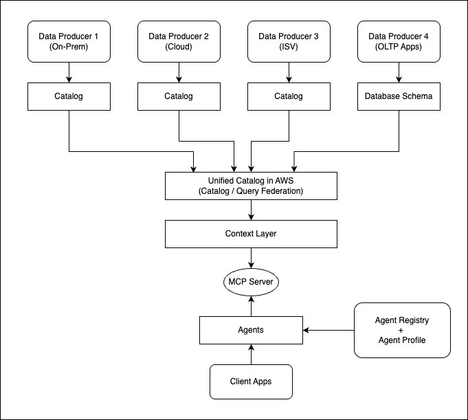
Architecture showing metadata catalogs and MCP servers onboarded to a context layer that feeds AI agents

If any of the data sources does not have a well-defined metadata catalog, you can define Model Context Protocol (MCP) servers on them, and then directly onboard them to the context layer. For example, if you have semi-structured or unstructured datasets for which you do not have a well-defined metadata catalog, or you want to onboard third-party data sources through REST APIs, then you can add their respective MCP server to the context layer directly. The following architecture explains the extended flow for it.
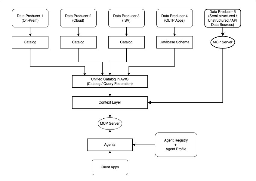
Extended architecture where data sources without a metadata catalog expose MCP servers directly to the context layer

In this series of posts, we demonstrate how you can unify the metadata catalog access across multiple providers, how you can enable AI agents to query the unified catalog, and how the context layer can be integrated to unify metadata from catalogs and MCP servers. We have divided the series into the following parts.

  • Part 1: Architecture approach with tradeoffs to unify a multi-cloud lakehouse architecture that can power Agentic AI (this post).
  • Part 2: Implementing an example solution to unify catalogs from multiple providers and deploy AI agents to query the unified data access layer.
  • Part 3: Integrate a context layer on top of the unified catalog for AI agents.
  • Part 4: Onboard additional data sources to the context layer through MCP servers and demonstrate the full solution.

This post focuses on explaining the architecture approach to build the open lakehouse architecture on AWS, unifying the metadata catalog across providers for the AI agents to access. In addition, it highlights the architecture trade-offs and best practices.

Use case

Every AI initiative launched on a fragmented data foundation is an initiative that will need to be rebuilt. Organizations that establish unified data access today are the ones that will scale Agentic AI with confidence tomorrow. Consider a large enterprise managing petabytes of data across a diverse set of environments:

  • On-premises: Network device telemetry, customer records, and operational databases.
  • Multiple cloud platforms: Marketing analytics, HR systems, and enterprise applications distributed across cloud providers.
  • Data platforms: Data science workloads, feature engineering pipelines, and finance and supply chain analytics running on specialized platforms.
  • SaaS applications: Salesforce, SAP, Zendesk, ITSM, and other business tools that each hold a critical piece of the enterprise data picture.

The business objective is to build a unified analytics and AI platform that can:

  • Query and analyze data across all environments without requiring full data migration.
  • Enforce consistent data governance and access control regardless of data location.
  • Power AI agents that can autonomously discover, query, and act on enterprise data.
  • Reduce total cost of ownership by eliminating redundant pipelines and storage.

This architecture directly addresses these needs by combining flexible data integration patterns, an open-table-format-based lakehouse architecture (with an example of Apache Iceberg), AI agent deployment to access unified metadata, and centralized governance.

Reference architecture

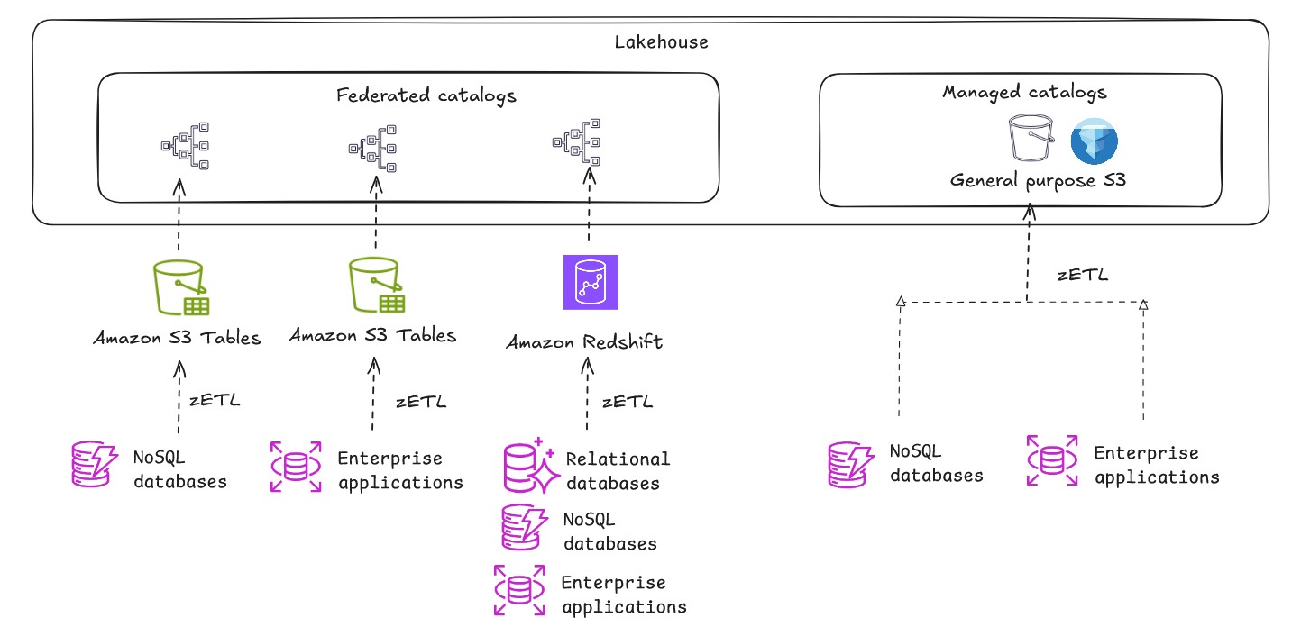
Before going deeper into a specific architecture, let’s revisit at a high level how the AWS open lakehouse architecture enables data ingestion and query or catalog federation to power analytics, machine learning development, and generative AI application development.

The following architecture diagram represents an end-to-end flow that includes:

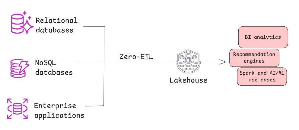
  • Data ingestion to the data lake or data warehouse through Zero-ETL and batch or stream processing using AWS native services, or accessing data from Google Cloud Platform using AWS Interconnect – multicloud.
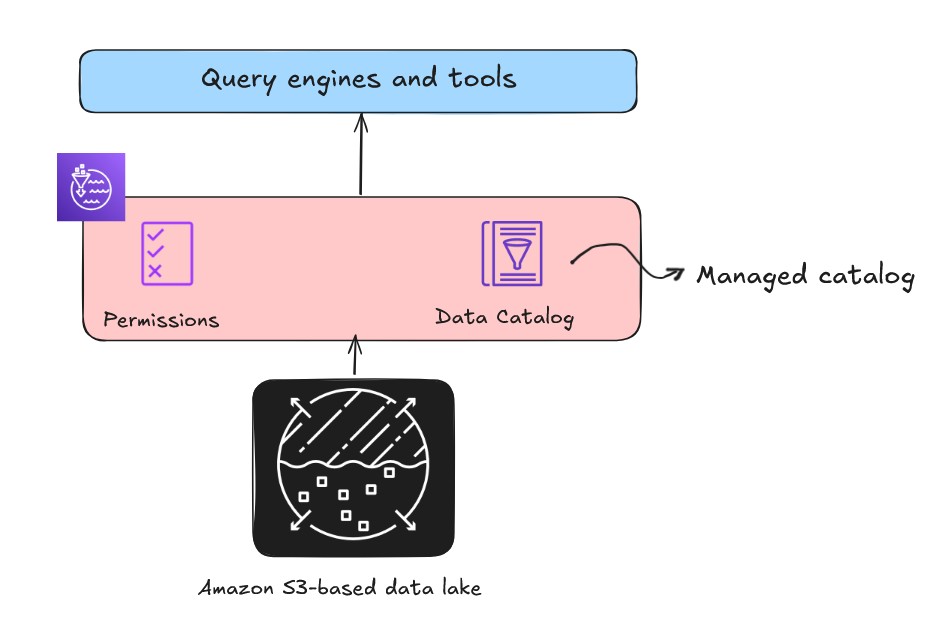
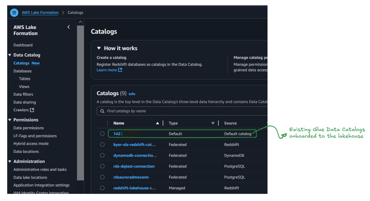
  • A centralized metadata catalog layer that includes data on AWS and metadata representation of non-AWS data sources using query or catalog federation.
  • A context layer that you can integrate to create a knowledge graph with ontology and business semantics that can enrich context for AI agents.
  • The consumption layer, which can include analytics, machine learning model development with Amazon SageMaker AI, and generative AI application development with Amazon Bedrock AgentCore, Amazon Quick, or other AWS and non-AWS AI applications.
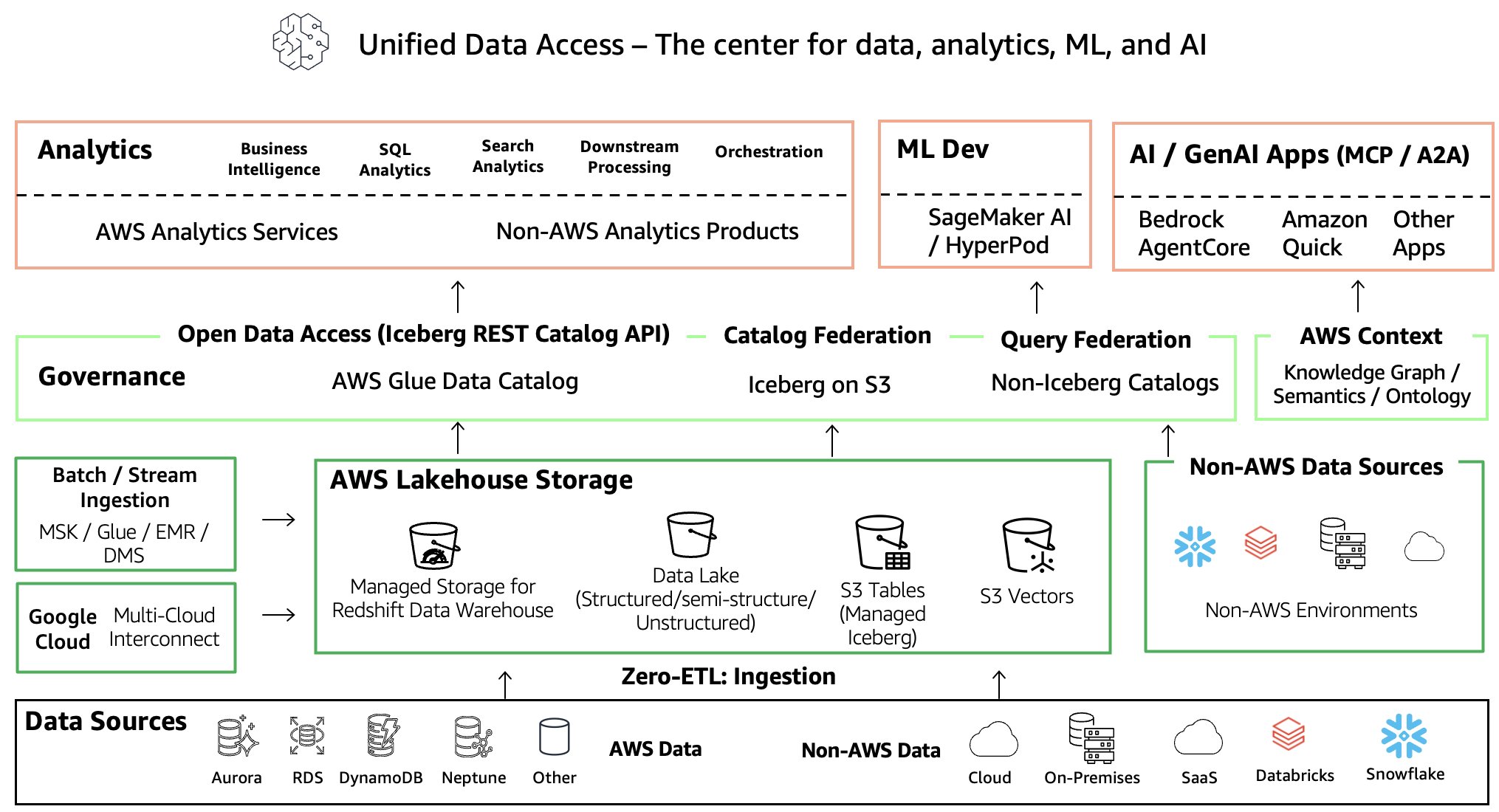
End-to-end AWS open lakehouse architecture spanning ingestion, catalog, context, and consumption layers

Let’s look at an expanded version of this architecture that details the data ingestion and data consumption patterns to build a unified data access layer on AWS that spans multiple cloud and ISV providers.

Expanded technical architecture walkthrough

The following architecture demonstrates the comprehensive AWS approach for metadata catalog consolidation through flexible integration patterns, and it also highlights patterns for building a lakehouse on AWS. Built on the open standards of Apache Iceberg for storage and governance through AWS Lake Formation, it creates a unified data foundation that connects existing investments without requiring wholesale migration, and it makes enterprise data AI-ready from day one. This architecture delivers value at every layer: business teams query across platforms without data movement, IT teams manage governance through a single federated layer with the flexibility to federate or ingest per use case, and compliance teams enforce policies once across all sources with full lineage and audit coverage.
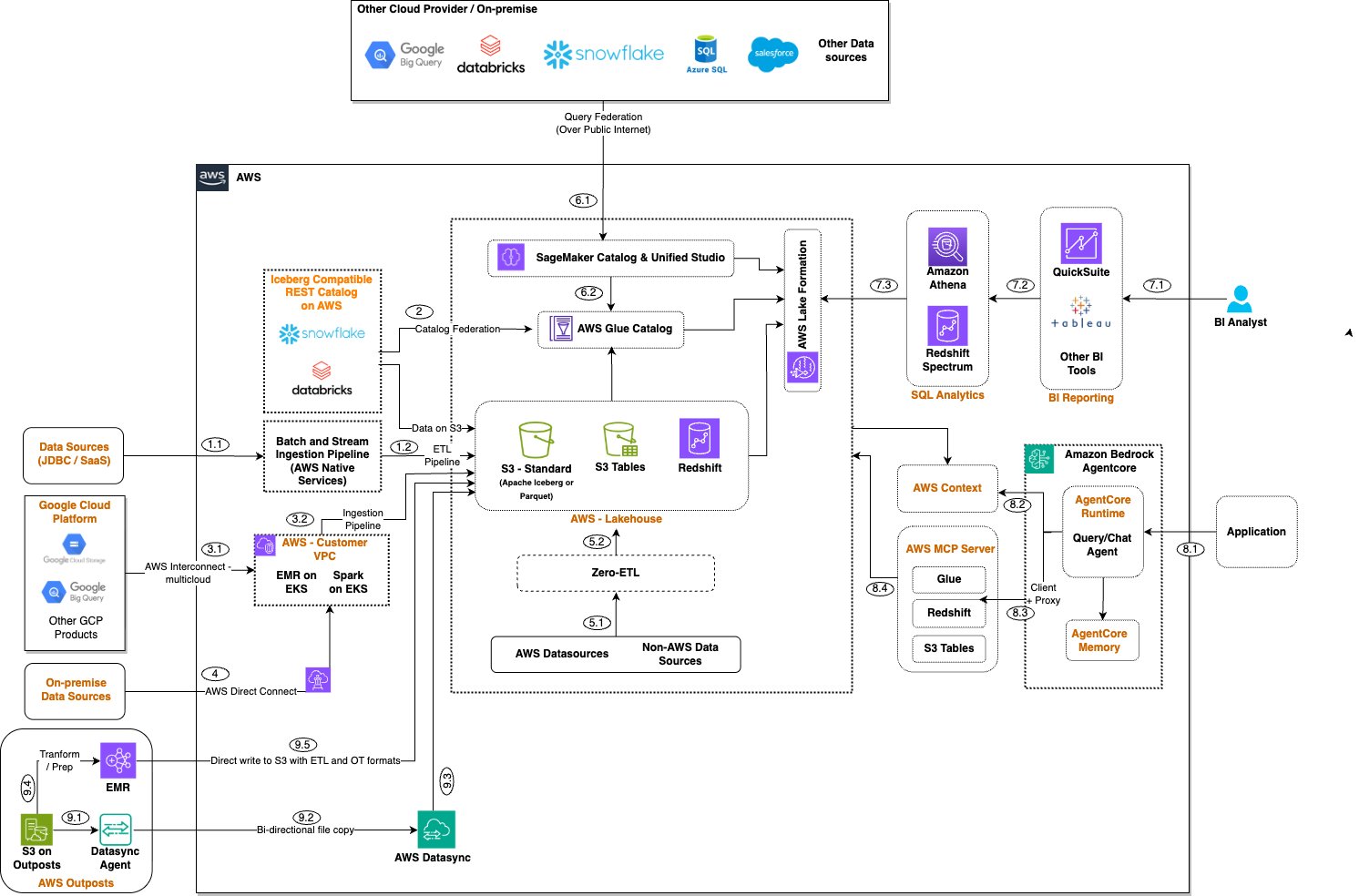
Expanded lakehouse architecture on AWS showing federation and ingestion patterns across multiple cloud and ISV providers

The following are the key components of the architecture.

Data access methods

This section provides options to access data that is not available in AWS Glue Data Catalog and not available on AWS.

1. Iceberg catalog federation (Reference points 2, 6.1, 6.2)

  • AWS Glue Data Catalog implements the Iceberg REST Catalog API specification, which enables seamless federation with Databricks, Snowflake, or other Iceberg-compatible catalogs set up with Amazon Simple Storage Service (Amazon S3) as the storage layer.
  • With the growing adoption of Apache Iceberg, catalog federation will become a common standard in the future and simplify metadata unification.

2. Query federation (Reference point 1.1)

  • Direct cross-cloud querying over the public internet to Google BigQuery, Azure SQL, Salesforce, and other platforms.
  • Real-time access to external data sources without replication, and seamless access with AWS analytics services.
  • Provides flexibility, because the catalog federation capability of the Iceberg REST catalog is limited to Iceberg tables only.

2.1. Secured private connectivity to Google Cloud Platform using AWS Interconnect for multi-cloud (Reference points 3.1, 3.2)

The default query federation approach makes the connection and transfers data over the public internet, which has its own latency implications depending on the target platform and the data volume transferred over the internet. During re:Invent 2025, AWS announced the public preview of AWS Interconnect – multicloud, which recently became generally available.

AWS Interconnect – multicloud is a managed service that provides private, high-speed, and secure network connections between Amazon Web Services (AWS) and other cloud providers, starting with Google Cloud Platform (GCP), with Microsoft Azure and Oracle Cloud Infrastructure (OCI) coming later in 2026. You can enable the integration with three steps: 1) specify the target cloud service provider, 2) select the destination Region on the other side, and 3) pick the required bandwidth.

The following architecture represents AWS and GCP integration with AWS Interconnect – multicloud.
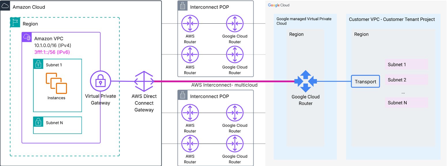
High-level architecture of AWS and GCP integration through AWS Interconnect for multi-cloud

On the AWS side, you need an AWS Direct Connect gateway (a global construct that acts as a route reflector), which you can attach to your Amazon Virtual Private Cloud (Amazon VPC) through a virtual private gateway or AWS Transit Gateway, or AWS Cloud WAN. On the GCP side, you need a Google Cloud Router that you attach to your customer VPC. Interconnect – multicloud offers pre-cabled capacity pools at shared Interconnect points of presence (PoPs) in selected Regions, where both AWS and GCP routers are co-located and pre-wired.

Because Interconnect – multicloud primarily routes traffic within the VPC through a private network, to benefit from it you need to keep your query engine or jobs within a customer VPC.

2.2. High network bandwidth with on-premises systems (Reference point 4)

  • AWS Direct Connect for high-bandwidth, low-latency on-premises connectivity.

Data ingestion methods

This section focuses on ways you can use to onboard datasets (complete or subset) to a lakehouse on AWS.

1. Zero-ETL: Data movement to AWS with Zero-ETL ingestion (Reference points 5.1, 5.2)

  • AWS Zero-ETL capabilities for seamless data loading from AWS and non-AWS sources.
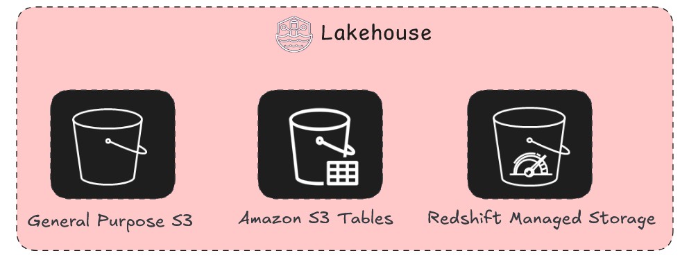
  • Flexibility to choose your target as an Amazon S3 based data lake or Amazon Redshift.

2. Extract, transform, load (ETL): Extract data from JDBC or SaaS sources and transform through a batch or stream pipeline (Reference points 3.1, 3.2)

The following architecture expands the flow 1.1 to 1.2 ingestion method that integrates AWS services to onboard data to the Amazon S3 raw layer and then takes it through an ETL pipeline for data cleansing and transformations. It also includes steps to onboard unstructured data to Amazon S3 using Amazon Bedrock Data Automation, and taking the lakehouse data for machine learning development with Amazon SageMaker AI.
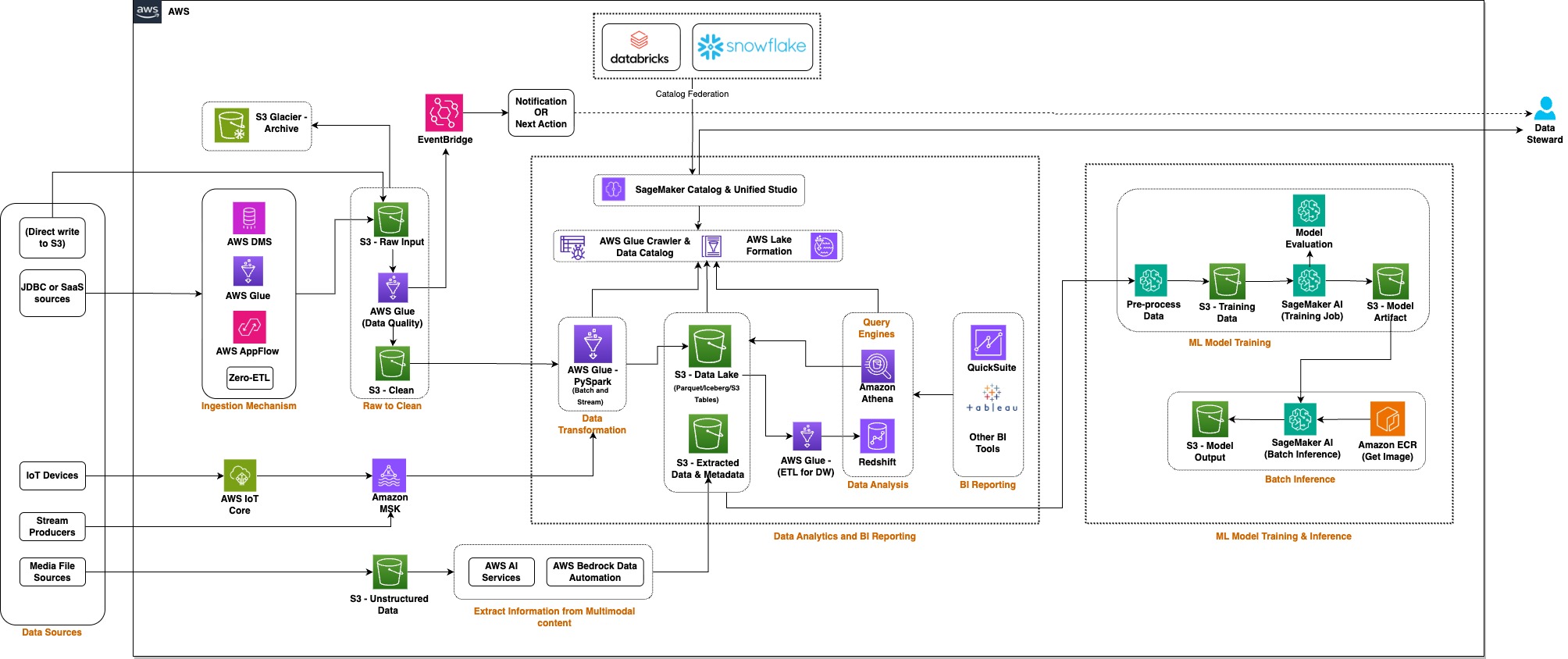
Ingestion architecture integrating AWS services to load data into the Amazon S3 raw layer and process it through an ETL pipeline

You can also use AWS Interconnect – multicloud to run Spark jobs (Spark with Amazon EMR on EKS or open source Spark on any compute within a customer VPC) to ingest and transform data from Google Cloud with private connectivity.

3. Accessing data from Google Cloud over a private network

Refer to the preceding data access methods (3.1 and 3.2).

4. Onboarding data from AWS Outposts (S3 on Outposts) (Reference points 9.1 to 9.5)

  • Option to onboard S3 on AWS Outposts data to regional Amazon S3 through AWS DataSync (reference 9.1 to 9.3), which might be a better fit to sync files as-is through a scheduled batch or an event-driven approach.
  • Flexibility to transform the S3 on Outposts data using an Amazon EMR clusters on Outposts job, and then directly write the transformed output to a regional Amazon S3 bucket in the formats you want (including open table formats such as Apache Hudi, Apache Iceberg, and Delta Lake).

Lakehouse foundation with Apache Iceberg

By standardizing on Apache Iceberg, you’re not choosing AWS over your other platforms. You’re choosing interoperability and future flexibility. Your data becomes truly portable across any Iceberg-compatible engine.

  • Open table format: Industry-standard format supported across AWS, Databricks, Snowflake, and other platforms, which eliminates vendor lock-in.
  • ACID transactions: Reliability with full transactional consistency.
  • Time travel and schema evolution: Built-in versioning and flexible schema management.
  • Performance optimization: Advanced features such as hidden partitioning, partition evolution, and metadata management.

Note that lakehouse storage is not limited to the Apache Iceberg format, and you have the flexibility to include other open table formats (for example, Apache Hudi and Delta Lake) or file formats (for example, Apache Parquet and Apache Avro).

Unified governance and access control

AWS governance capabilities transform the lakehouse from a storage layer into a fully governed data platform. This delivers security, compliance, and data quality out of the box, applied consistently across all data sources including federated catalogs. A unified catalog consolidates metadata from AWS and non-AWS sources with generative AI-powered business glossary generation, while automated ML-powered classification identifies sensitive data (for example, PII, PHI, and financial data) across structured and unstructured datasets. AWS Identity and Access Management (AWS IAM) and AWS Lake Formation enforce fine-grained access control at the row, column, cell, and tag level, applied consistently across Amazon Athena, Amazon Redshift Spectrum, Amazon EMR, and federated sources. End-to-end data lineage tracking provides visual data flow graphs, impact analysis, and compliance audit trails. When AI agents explore metadata from the unified catalog and submit a query to Amazon Athena for execution, the Lake Formation fine-grained access control filters data based on the user interacting with the AI agent.

For the foundation model integrated into your AI agents, you can use Amazon Bedrock Guardrails, which implements customized safeguards to block harmful content and minimize hallucinations. Amazon Bedrock AgentCore provides fine-grained policy control over agent actions with real-time enforcement and managed authentication for agents accessing AWS and third-party services.

A comprehensive audit and compliance stack spans Amazon CloudWatch, AWS CloudTrail, AWS IAM, AWS Key Management Service (AWS KMS), AWS Audit Manager, and AWS PrivateLink. This stack makes sure every agent invocation is traceable, every key is managed, and every configuration is automatically mapped to frameworks including ISO, SOC, GDPR, and HIPAA.

When an end user interacts with the AI chat assistant, the layers of security and governance should go through the following.

Layer 1: Who can access?

  • Enable Active Directory and single sign-on integration for user authentication, and a combination of AWS IAM roles for AWS API-level authorization.

Layer 2: What can they see?

  • Integrate an agent profile to define what datasets each agent can access, because not all agents should have access to all datasets.
  • Enable fine-grained access control on the metadata layer using AWS Lake Formation that can filter rows and columns.
  • Enable data masking as applicable while the query responses are served through the query engine.

Layer 3: What can the agent do?

  • Control agent actions by restricting them to read-only, and apply restrictions to INSERT, UPDATE, and DELETE if the agents are supposed to query only.
  • Apply a limit on the number of rows that can be returned from the query, and apply a query scan limit to reduce cost.

Layer 4: What does the agent reveal?

  • Enable output filtering to make sure no PII is included.
  • Apply Amazon Bedrock Guardrails on large language model (LLM) responses to make sure the model does not produce anything inappropriate.
  • In addition, enable audit logging of all queries to make sure future audit and compliance needs can be met.

Comprehensive analytics ecosystem (Reference points 7.1, 7.2, 7.3)

AWS offers a complete analytics ecosystem that includes the following.

  • Amazon Athena: Serverless SQL queries with Iceberg v2 support, including provisioned capacity for consistent performance and workgroups for resource and cost management.
  • Amazon Redshift Spectrum: Federated queries across the data warehouse and Iceberg data lake.
  • Amazon Quick Sight: Enterprise visualization with governed access to all data.
  • AWS Glue and Amazon EMR: Distributed data processing capability for enterprise transformations.

AI-ready architecture (Reference points 8.1 to 8.4)

A consolidated lakehouse architecture helps you make data ready for AI agents that can access the data through readily available MCP servers or through the AWS SDK for Python (Boto3) for Amazon Athena or Amazon Redshift Spectrum. AI agents can integrate the AWS MCP Server to interact with AWS analytics services such as AWS Glue, Amazon Athena, and Amazon S3 Tables, a capability of Amazon S3, to query both data and metadata.

AI agents need context to understand how the catalog tables and their attributes are linked to each other, how users have queried them in the past, or what priorities are defined to understand which one is an authoritative source for a particular natural language question. To enable the AI agent with additional context, we can integrate the AWS Context service that was pre-announced recently at the AWS New York Summit 2026.

Governance integration: AI agents automatically inherit Lake Formation permissions, because the agent can submit the SQL query to be run through Amazon Athena or Amazon Redshift Spectrum. This makes sure they only access data that users are authorized to see. Amazon SageMaker Unified Studio data lineage tracks AI agent queries for full auditability.

The following diagram represents how the AI agent request flow looks.
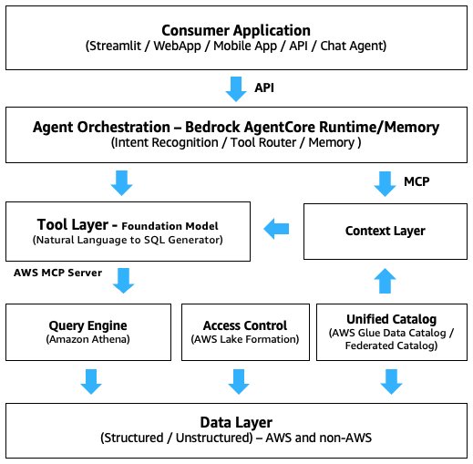
AI agent request flow through the unified catalog, Lake Formation governance, and Amazon Athena

This architecture delivers value across every layer of the organization. Business teams gain faster time-to-insight by querying data across all platforms without waiting for data movement, while eliminating duplicate storage and reducing transfer costs through federation. The Apache Iceberg open table format ensures data portability and freedom from vendor lock-in. For IT and data teams, a single governance layer across all sources, including federated catalogs, reduces operational complexity, while the flexibility to choose between federation and ingestion for each use case, combined with the elastic AWS infrastructure and the petabyte-scale metadata architecture of Iceberg, delivers both agility and scalability. Data governance and compliance teams benefit from a single point of policy enforcement across all data regardless of location, complete lineage and access logs for audit and compliance reporting, automated sensitive data classification, and policies that are defined once and enforced everywhere, including across federated sources.

Architecture tradeoffs and best practices

The following are a few key trade-offs you need to consider while designing the solution.

Data ingestion and access methods

Use catalog federation (Iceberg REST) when:

  • The source platform supports the Iceberg REST API (Databricks, Snowflake Polaris).
  • Data is already in Iceberg format with Amazon S3 backed storage.
  • You want bidirectional discovery (AWS tables visible in Databricks or Snowflake too).

Use query federation (Amazon SageMaker Lakehouse architecture or AWS Glue connectors) when:

  • The source is BigQuery, SQL Server, or another non-Iceberg platform.
  • Data must stay in the source cloud (sovereignty, contractual, or latency reasons).
  • Real-time access is required without replication lag.

Use ingestion (Zero-ETL, AWS Glue, or Amazon EMR) when:

  • Data is accessed frequently with a low-latency requirement by AI agents or high-concurrency analytics.
  • The business decides to build a data lake and warehouse on AWS.
  • You need full governance, time travel, and performance optimization.

Use AWS Interconnect – multicloud when:

  • You need real-time or near-real-time query federation to GCP data sources (BigQuery, AlloyDB, Cloud Spanner) and latency or security requirements prohibit public internet routing.
  • You have high-volume, recurring data transfers between AWS and GCP where public internet egress costs or bandwidth variability are unacceptable.
  • Your organization has compliance or regulatory requirements mandating that data never traverse the public internet (HIPAA, PCI-DSS, or financial services regulations).
  • You need bidirectional connectivity, such as GCP workloads calling AWS APIs, or AWS workloads calling GCP APIs, both over private paths.

Choosing between federation and ingestion based on use case

Dimension Federation (Query in Place) Ingestion (Move to AWS)
Data freshness Real-time or near-real-time Dependent on ingestion frequency
Query performance Subject to source system latency and network Subject to data volume and operation, avoids cross-cloud network latency
Cost Lower storage cost. Higher per-query cost for cross-cloud egress Higher upfront ingestion cost. Lower ongoing query cost
Governance Partial. Source system retains some control, and a unified catalog can simplify governance for consumers Full. Lake Formation enforces all policies across all AWS analytics services
Data portability Data remains in source Data fully portable in open format
AI readiness Limited. Agents depend on source availability High. Agents query optimized, governed Iceberg tables
Operational complexity Lower initial setup. Harder to debug cross-cloud issues Higher initial setup. Simpler long-term operations

Integrating Amazon Bedrock AgentCore Gateway and Amazon Bedrock AgentCore Runtime based on use case

The following are key differences between AgentCore Gateway and AgentCore Runtime that are relevant for our use case.

Dimension Amazon Bedrock AgentCore Gateway Amazon Bedrock AgentCore Runtime
Timeout 5 minutes (hard limit) 15 min sync / 8 hours async
Statefulness Stateless (per-request) Stateful (session-based)
Best for Lightweight API proxying Long-running data processing
Your lakehouse queries Will time out frequently Handles multi-hour jobs

Because AgentCore Gateway has a 5-minute hard timeout limit, use AgentCore Runtime for data processing jobs.

  • AWS Glue ETL jobs can run for minutes to hours.
  • Amazon Redshift queries on large datasets routinely exceed 5 minutes.
  • Athena federated queries (especially cross-cloud through Interconnect) can be slow.
  • Iceberg table scans on multi-TB datasets take time.

You can use AgentCore Gateway if the scope is limited to Glue Data Catalog interactions to fetch metadata schema, because that won’t run for more than 5 minutes.

Design considerations for production implementation

In practice, there are multiple aspects to consider when deploying the solution for production. The following summarizes a few of the key issues you might encounter and approaches to address them.

Catalog federation: The metadata drift problem

One of the first surprises in production is metadata drift, the state where your federated catalog no longer reflects the actual schema of the source system, because the source system’s metadata changes are not reflected in the unified catalog. The agent continues to generate SQL against the stale schema, producing silent failures that are hard to trace.

The following are a few ways you can address the metadata drift issue.

  • Implement a catalog refresh schedule. Even a daily Glue crawler run against federated sources catches most drift before it causes agent failures.
  • Add schema validation as a pre-query step in your agent tool. Before running SQL, verify that the referenced columns exist in the current catalog metadata.
  • Instead of pulling metadata changes from the source in a scheduled manner, you can design an event-driven system, where the source system triggers a push event to run the schema change in the federated catalog.

Query federation: Latency is non-deterministic

Query federation works well for moderate data volumes, but latency becomes non-deterministic at scale. A query that returns in 3 seconds during testing can take more than 10 seconds in production when the source system is under load, the network path is congested, or the federated connector is cold-starting.

The following are a few approaches you can consider to improve the performance.

  • Set explicit query timeouts in your Athena execution context. Without them, a slow federated query will block your agent indefinitely.
  • Implement query result caching for frequently asked questions. Most business users ask the same questions repeatedly, and caching at the agent layer improves perceived performance.
  • For time-sensitive use cases, consider caching aggregated data in an AWS lakehouse on a schedule rather than querying live. This trades freshness for reliability.

AgentCore memory: Statefulness cost

AgentCore Memory enables stateful conversations, but in production, unbounded memory accumulation creates its own problems. An agent that remembers every conversation eventually starts surfacing stale context. For example, a user who asked about Q3 revenue six months ago gets that context injected into a Q1 query today.

The following are a few ways you can optimize cost and improve relevance.

  • Set explicit memory expiry (we use 30 days as shown in the implementation) and enforce it consistently.
  • Use session-scoped memory for transactional queries and long-term memory only for user preferences and recurring patterns.
  • Implement a memory review step in your LangGraph workflow. Before invoking the model, filter retrieved memories by recency and relevance score rather than injecting all of them.

LangGraph orchestration: When tool calls loop

The conditional routing of LangGraph is powerful, but in production we observed a failure mode where the agent enters a tool call loop. The model repeatedly calls the same tool with slightly different parameters, never reaching a satisfactory answer. This typically happens when the tool returns partial or ambiguous results and the model keeps trying to refine.

What we learned:

  • Add a maximum tool call counter in your LangGraph state. If the agent has called tools more than N times in a single session, force a graceful exit with a summary of what was found.
  • Return structured, unambiguous responses from your tools. Include row counts, column names, and explicit null indicators so the model can reason clearly about completeness.
  • Log every tool invocation with its input and output. This is the single most valuable debugging artifact when diagnosing agent misbehavior in production.

Handling hallucination risks in federated agent architectures

This is the most important section for teams moving from prototype to production. Hallucination in agentic AI systems that query real data is qualitatively different from hallucination in general-purpose LLMs, and it is more dangerous because the outputs look authoritative.

There are three distinct hallucination risk zones in a lakehouse AI agent:

  • SQL generation: The model generates SQL that is syntactically valid but semantically wrong. For example, when asked “What is our revenue growth this quarter?”, the model might generate a query that compares the wrong date ranges, uses the wrong aggregation function, or joins tables on incorrect keys, and then returns a confident, formatted answer with the wrong numbers.
  • Cross-source synthesis: When the agent queries multiple federated sources and synthesizes results, the risk compounds. The model may correctly retrieve customer counts from Amazon S3 and revenue figures from Snowflake, but incorrectly draw conclusions that aren’t supported by either dataset individually.
  • Memory-augmented reasoning: When long-term memory is active, the model may blend historical context with current query results in ways that are factually incorrect. For example, it might apply a business rule that was true six months ago but has since changed.

To improve, before any agent output informs a business decision, apply the following three-step validation framework:

  • Step 1: Source verification. Can you trace the answer back to a specific table, column, and row count? If the agent can’t show you the SQL and the row count, the answer is unverified.
  • Step 2: Reasonableness check. Does the answer fall within expected ranges? A sudden 10x spike in customer count is a signal to investigate.
  • Step 3: Cross-validation. For critical decisions, run the equivalent query directly in Athena or your BI tool and compare. Discrepancies reveal either a model reasoning error or a data quality issue. Resolve both before the answer is trusted.

These lessons don’t diminish the value of the architecture. They make it production-ready. The teams that move fastest with agentic AI are not the ones who skip these guardrails. They’re the ones who build them in from the start and spend less time firefighting in production.

Alternative to the unified catalog approach

In case you face technical and process challenges to unify catalogs across providers, you can let each data producer expose the metadata and data through MCP servers, as represented in the following diagram. In this approach, each producer takes the responsibility of maintaining the MCP servers and exposing them to the context layer. While this approach provides autonomy to data owners to operate independently and with flexibility, it also creates operational overhead to synchronize all metadata in a consistent way.
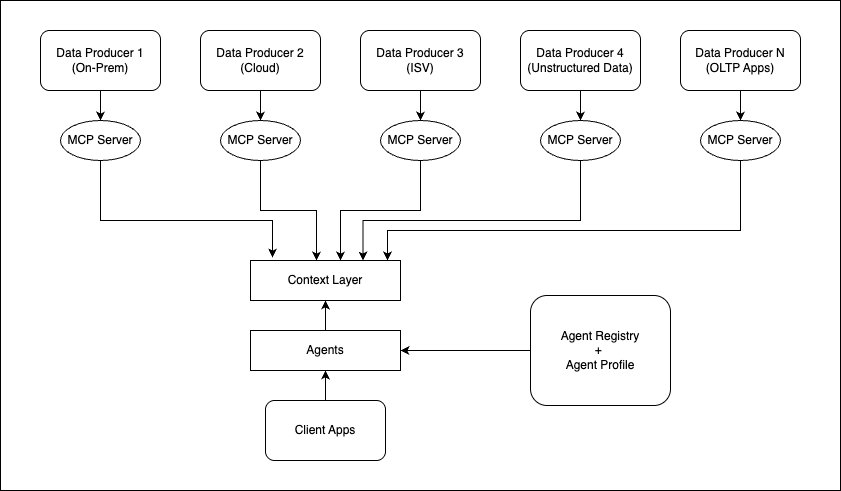
Alternative architecture where each data producer exposes its metadata and data through its own MCP server to the context layer

What’s next

In Part 2 of this series, we walk through the full implementation step by step, including hands-on scripts to:

  • Load example sales datasets into Databricks and marketing data to Snowflake as Iceberg tables, and federate them into AWS Glue Data Catalog through the Iceberg REST API.
  • Register Google BigQuery as a native federated data source in Amazon SageMaker, instead of a traditional AWS Lambda connector integration.
  • Create a customer master table as a native Iceberg table in Amazon S3.
  • Run a single SQL query in Amazon Athena that joins all four sources across two federation patterns, with no data movement.
  • Deploy an AI agent on Amazon Bedrock AgentCore that can autonomously query the same unified catalog using Amazon Athena and answer complex business questions in natural language queries. In addition, integrate AgentCore Memory to persist user context.

Conclusion

In this post, we summarized how you can unify data access across multiple cloud and ISV providers on AWS with the combination of catalog federation, query federation, and data movement to AWS. We then explained how AWS Glue Data Catalog and Lake Formation help provide unified catalog and access governance, and how AI agents hosted in Amazon Bedrock AgentCore can access it using MCP servers to explore the metadata context, convert user natural language queries to SQL, and use Amazon Athena to run the query across data sources to get the response to the end user. In addition, we provided an overview of different data ingestion methods to build a lakehouse architecture on AWS, including AWS Interconnect – multicloud and where it adds value.

We also provided architecture trade-offs and best practices to integrate the service capabilities. In the next post (Part 2), we will take a specific use case and provide a step-by-step implementation guide to unify the catalog and deploy the agent to Amazon Bedrock AgentCore.
About the author

Sakti Mishra

Sakti Mishra

Sakti is a Principal Data and AI Solutions Architect at AWS, where he helps customers modernize their data architecture and define end-to-end data strategies, including data security, accessibility, governance, and more. He is also the author of Simplify Big Data Analytics with Amazon EMR and AWS Certified Data Engineer Study Guide. Outside of work, Sakti enjoys learning new technologies, watching movies, and visiting places with family. You can connect with Sakti through his LinkedIn profile.

Deploy modern data platforms in minutes with MDAA

Post Syndicated from Sudeshna Dash original https://aws.amazon.com/blogs/big-data/deploy-modern-data-platforms-in-minutes-with-mdaa/

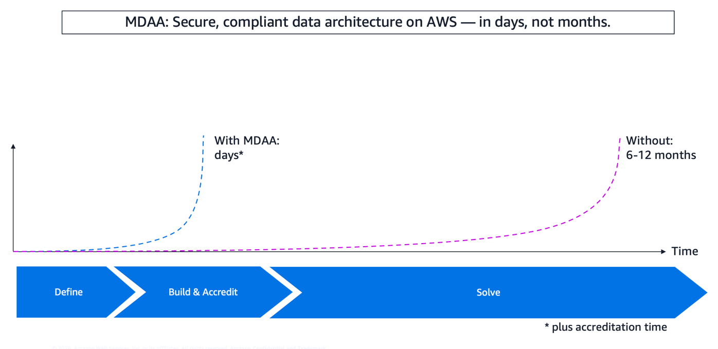
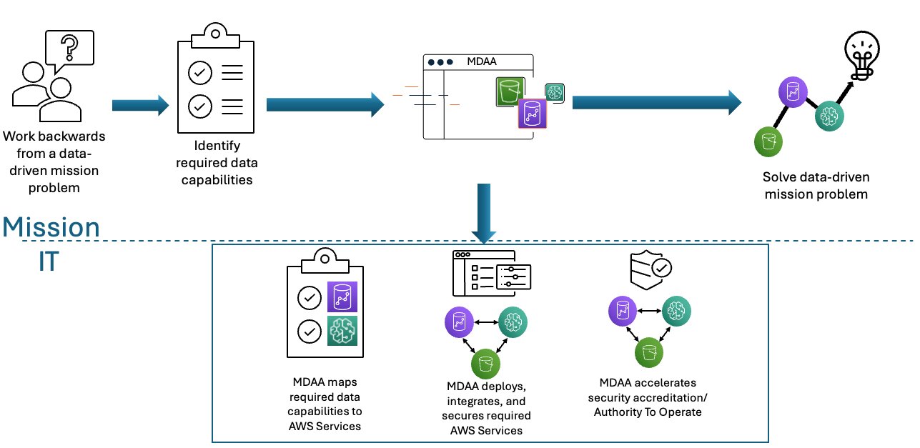
Modern Data Architecture Accelerator (MDAA) is an open source framework that replaces infrastructure code with concise YAML configuration, so your team can deploy a governed, production-ready data architecture, reducing deployment time from months to weeks (depending on complexity and team experience).

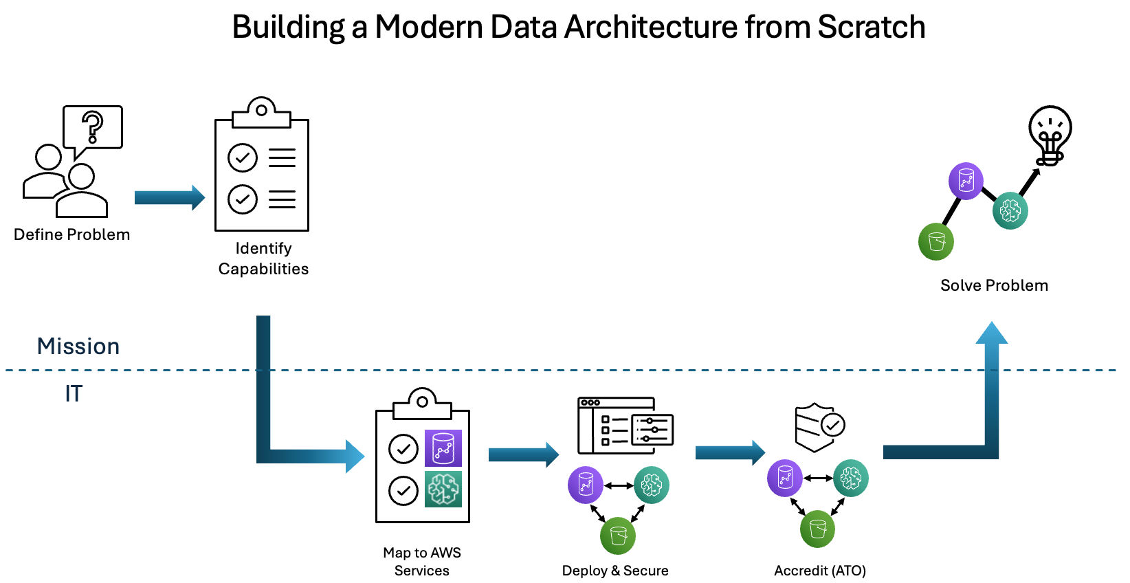
Organizations building modern data architecture on AWS face a critical challenge: deploying production-ready, governed infrastructure traditionally requires 6–12 months of custom development, thousands of lines of infrastructure code, and continuous remediation cycles to maintain security and compliance. Governance is often added incrementally, treated as an afterthought that creates compliance gaps and engineering rework.

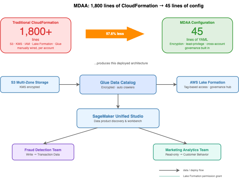
MDAA addresses this by replacing infrastructure code with concise YAML configuration, achieving up to 97.6 percent code reduction (from approximately 1,800 lines of AWS CloudFormation to 45 lines of MDAA YAML) while embedding governance from the start. The complete Governed Lakehouse Starter Kit deploys 491 AWS resources across 12 stacks from approximately 450 lines of YAML configuration, representing a 66x verbosity ratio where each line automatically expands into production-ready infrastructure.

In this post, we explore how MDAA transforms data architecture development from months of manual coding to production-ready deployment through configuration-driven infrastructure and embedded governance, examine a real customer transformation, and provide a clear implementation pathway for your own data modernization journey.

Customer use case and challenge

A university system office needed to modernize its analytics architecture across 17 campuses while managing sensitive educational data. Their third-party dependency created bottlenecks that slowed feature implementation from weeks to months, and their IT team lacked the cloud skillsets to build modern infrastructure independently.

With MDAA, they achieved:

  • 95 percent reduction in time-to-value for dashboard and feature implementation (from weeks to hours).
  • 17 campuses integrated into a unified, secure architecture.
  • 7.2TB of data and over 8,000 dashboards migrated successfully.
  • Significant cost savings by removing third-party dependencies and reducing license costs.
  • Enhanced security posture for external stakeholders accessing sensitive educational data.

The team used MDAA to implement a modernization strategy with continuous integration and continuous delivery (CI/CD) for automated deployment. The architecture now supports rapid response to stakeholder requests while maintaining strict data governance through AWS Lake Formation.

Their transformation demonstrates what becomes possible when governance is embedded from launch rather than added incrementally, moving from months-long manual development to weeks of production-ready deployment through configuration-driven infrastructure.

Solution: MDAA and its value propositions

MDAA’s capabilities stem from its modular, composable architecture. The accelerator provides over 40 pre-built modules that encapsulate AWS best practices for security, governance, and operational excellence. Organizations describe the outcomes they want in MDAA-specific YAML configuration files (not CloudFormation or Terraform YAML) and the accelerator automatically translates these configurations into AWS Cloud Development Kit (AWS CDK) constructs, which then deploy via CloudFormation with embedded governance.

Configuration over code. The MDAA framework takes a fundamentally different approach: describe the outcomes you want in YAML, and the accelerator deploys production-ready infrastructure with embedded governance. Consider deploying a governed data lake where fraud detection teams need write access to transaction data, while marketing analytics teams require read-only access to customer behavior data. Traditional approaches require over 1,800 lines of CloudFormation across Amazon Simple Storage Service (Amazon S3) buckets, AWS Key Management Service (AWS KMS) keys, AWS Identity and Access Management (IAM) policies, and Lake Formation permissions. With MDAA, the same governed data lake is expressed in 45 lines of configuration, a 97.6 percent reduction, while helping you apply encryption, least-privilege access, and cross-account governance as built-in defaults.

The configuration deploys multi-zone S3 storage with KMS encryption, Lake Formation permissions with tag-based access control (TBAC) enabled, Amazon SageMaker Unified Studio for data product discovery, and encrypted AWS Glue Data Catalog with automated crawlers. All permissions flow through Lake Formation rather than individual IAM policies.

Embedded governance from day one. Governance is declared in YAML and deployed alongside infrastructure from the first run. Fine-grained access controls, encrypted data catalogs, data quality validation, audit trails, and sensitive data classification are all part of the same configuration. MDAA’s Governed Lakehouse starter kit defines an entire governed data architecture in roughly 450 lines of YAML, which produces approximately 29,700 lines of CloudFormation across 12 stacks (a 98.5 percent reduction in infrastructure code).

Modular, composable architecture. Each module is purpose-built to handle a specific capability within the data architecture. Modules communicate through AWS Systems Manager Parameter Store, passing resource identifiers (Amazon Resource Names (ARNs), IDs, and names) between stacks. This approach removes hardcoded dependencies. A KMS key created in one module can be referenced by another through parameter resolution, with all dependencies resolved automatically at deployment time.

The diagram illustrates the deployed architecture and team-level access flow that MDAA generates from the 45-line configuration.

Progressive architecture patterns. MDAA provides four reference architecture patterns that align to progressive stages of data infrastructure maturity:

  • Basic Data Lake deploys a governed data lake with built-in security controls, data quality checks, centralized metadata management using AWS Lake Formation and AWS Glue.
  • Data Science Platform extends the data lake with Amazon SageMaker notebooks, feature stores, and machine learning (ML) pipelines so data science teams can experiment and train models on governed data.
  • SageMaker Unified Studio adds a single interface for analytics and ML collaboration, connecting data engineers, analysts, and data scientists in one workspace.
  • Generative AI Platform layers Amazon Bedrock and Retrieval Augmented Generation (RAG) capabilities on top of your existing data foundation, so teams can build generative AI applications grounded in enterprise data.

Each pattern builds the one before it. You can start with the Basic Data Lake and adopt additional patterns as your team’s needs grow. MDAA’s modular design means you add capabilities without rearchitecting what you already deployed.

The infrastructure is versioned through GitHub, repeatable across environments, and auditable through comprehensive AWS CloudTrail logging. Data engineers focus on data pipelines and business logic while MDAA manages infrastructure complexity and governance integration. This represents the fundamental shift: from writing infrastructure code to describing the outcomes you want through configuration, with governance embedded from the start.

Use case of MDAA: Governed data architecture

DataOps teams spend significant time on governance tasks, including permissions management, compliance validation, and access control, rather than building pipelines and analytics. These aren’t data problems, they’re governance problems that consume engineering capacity meant for higher-value work. MDAA addresses this at the architectural level. Governance is declared in YAML and deployed alongside infrastructure from the first run.

The following sections walk through how each governance module works in practice.

Publish, discover, subscribe, and consume data products between business units: SageMaker Unified Studio

Amazon SageMaker Unified Studio provides a governed data catalog where data producers publish data products, and consumers discover and subscribe to them. Your deployment with MDAA includes a pre-configured domain, blueprints (managed and custom), projects, and environment profiles, all defined in a single configuration file:

# sagemaker.yaml --- 16 lines that deploy 114 CloudFormation resources
domains:
  domain1:
    dataAdminRole:
      id: ssm:/{{org}}/govern1/generated-role/data-admin/id
    description: SMUS Domain 1
    userAssignment: MANUAL

    tooling:
      vpcId: '{{context:vpc_id}}'
      subnetIds:
        - '{{context:private_subnet_id1}}'
        - '{{context:private_subnet_id2}}'

    groups:
      team1:
        ssoId: '{{context:team1-group-sso-id}}'
      team2:
        ssoId: '{{context:team2-group-sso-id}}'

Behind this configuration, MDAA deploys an Amazon SageMaker Unified Studio domain with dedicated KMS keys, execution and provisioning roles, and single sign-on group profiles for team access. Data producers tag and publish assets with metadata, ownership, and classification. Consumers browse a searchable catalog, see only authorized assets, and request access through a governed workflow. Cross-account and cross-business-unit data sharing flows through a subscription model, ensuring every access grant is tracked, auditable, and revocable.

Use case of MDAA: Restricting access to cardholder data using Lake Formation

AWS Lake Formation provides fine-grained access control at database and table levels, removing manual IAM policy management. MDAA deploys AWS Lake Formation with pre-configured settings that disable IAMAllowedPrincipals, the critical governance setting that ensures all permissions flow through centralized governance:

# lakeformation-settings.yaml --- 6 lines that deploy 25 CloudFormation resources
lakeFormationAdminRoles:
  - id: generated-role-id:data-admin
createCdkLFAdmin: true
createDataZoneAdminRole: true
iamAllowedPrincipalsDefault: false

That last flag is the single most important governance setting in the platform. Without it, an IAM principal with glue:GetTable can read tables in the catalog, bypassing the entire access control model. Most manual setups miss this or defer it.

With the data lake configuration, you declare roles and access policies in YAML where admins get full control, engineers get read access to curated data, extract, transform, and load (ETL) roles get scoped write access, and MDAA compiles them into the correct S3 bucket policies and Lake Formation registrations.

Use case of MDAA: Ensuring data integrity with AWS Glue Data Quality

AWS Glue Data Quality runs automated validation rulesets continuously as part of the pipeline, not as periodic batch checks. MDAA’s data quality module supports over 15 built-in rule types, from completeness and uniqueness checks to statistical thresholds and data freshness validation:

# data-quality.yaml
projectName: example-project

rulesets:
  customer-data-quality:
    description: Validate customer data completeness and uniqueness
    targetTable:
      databaseName: project:databaseName/customer-data
      tableName: customers
    ruleset:
      - ruleType: IsComplete
        column: customer_id
      - ruleType: Uniqueness
        column: email
        comparisonOperator: ">"
        threshold: 0.95
      - ruleType: RowCount
        comparisonOperator: ">"
        value: 100

Quality metrics flow into Amazon CloudWatch for real-time alerting. If anomalies are detected, automated workflows quarantine affected records and alert data engineering teams before issues reach downstream consumers.

Protecting metadata at rest: AWS Glue Data Catalog encryption

Table schemas, column names, and partition structures can reveal sensitive information about an organization’s data architecture, even without access to the underlying data. AWS Glue Catalog Encryption secures metadata at rest using AWS KMS-managed keys. MDAA configures catalog encryption by default, so schema definitions and connection passwords are encrypted from initial deployment without requiring manual key management setup. Access to catalog metadata follows the same Lake Formation governance controls applied to the data itself, so teams see only the schemas that they’re authorized to query.

Auditing every data access event: CloudTrail integration

Every data access event must be logged and attributable to a specific identity. Without a complete audit trail, demonstrating compliance during a regulatory review becomes a manual, error-prone process. AWS CloudTrail captures API-level activity across the data infrastructure, recording who accesses what data, when, and from which service. MDAA configures CloudTrail integration by default, so audit logging is active from initial deployment rather than added retroactively. Log data flows into a centralized, tamper-resistant store, giving compliance teams a single location to query access history across all business units and accounts.

Identifying sensitive data automatically: Macie integration

In large environments, sensitive information spreads across dozens of S3 buckets through pipelines, transforms, and ad hoc data drops, and self-reporting data owners consistently produce gaps. Amazon Macie uses machine learning to automatically discover and classify sensitive data in S3, surfacing findings at the object level without manual tagging. MDAA configures Macie across your S3 buckets during deployment, routing findings to Amazon EventBridge where automated workflows can alert owners or trigger remediation.

Together, these controls form a layered defense: Lake Formation governs access to cataloged data, Glue Data Quality validates integrity on arrival, and Macie identifies sensitive data that lands outside governed pipelines to reduce compliance risk.

Multi-account data mesh

MDAA provides extensive support for multi-account data mesh setups, with decentralized data ownership across business units and centralized governance. The data mesh starter kit supports cross-account data product publishing and consumption, allowing organizations to scale data sharing while maintaining consistent security and compliance controls.

Technical implementation

Ready to deploy your modern data architecture? Here are the resources to get started:

MDAA Implementation Guide provides detailed instructions for deploying all starter packages, including architecture patterns, configuration examples, security best practices, and troubleshooting guidance.

MDAA Hands-on Workshop offers step-by-step guided implementation with AWS experts. The workshop covers configuration management best practices, implementation patterns, hands-on labs with real-world scenarios, and cleanup instructions.

GitHub Repository and Documentation provide source code, module reference, and comprehensive documentation.

Organizations approach MDAA from different starting points. Some modernize existing data architectures, migrating from on-premises infrastructure or legacy cloud architectures. Others build new architectures for artificial intelligence and machine learning (AI/ML) initiatives or generative AI applications. Financial services organizations require PCI-DSS compliance from day one. Healthcare organizations need controls that can help support HIPAA. Each journey benefits from MDAA’s configuration-driven approach and embedded governance.

Conclusion

MDAA transforms data architecture development from months of manual coding to production-ready deployment. Configuration-driven infrastructure reduces development time by 40–60 percent while embedding governance from the start. The university system’s 95 percent reduction in time-to-value demonstrates the outcome: organizations deploy secure, compliant, governed data architectures in weeks rather than months.

Financial services organizations can deploy architectures to help them align with PCI-DSS compliance requirements using Lake Formation access controls, Glue Data Quality validation, SageMaker Unified Studio data discovery, comprehensive CloudTrail audit trails, and automated Macie data classification, all inherited from configuration rather than built manually.

Data architecture journeys need not follow six-month timelines with governance added incrementally. MDAA provides an alternative: describe the outcomes you want through YAML configuration, inherit pre-validated security controls, and deploy production-ready infrastructure with comprehensive governance from initial deployment.

Security and compliance is a shared responsibility between AWS and the customer. For more information, see the AWS Shared Responsibility Model.

Need help or have questions? Contact AWS ProServe for personalized guidance on selecting the right package and deployment strategy for your organization.


About the author

Sudeshna Dash

Sudeshna Dash

Sudeshna is a Data Scientist at AWS Professional Services based in Berlin, Germany. She specializes in data architecture, generative AI, and agentic AI systems on AWS. Sudeshna is a contributor to the Modern Data Architecture Accelerator (MDAA) open-source project and helps customers design and deploy governed, production-ready data and AI/ML architectures on AWS.

John Reynolds

John Reynolds is a Principal Engineer with AWS Professional Services based in Seattle, Washington. He leads the architecture and development of Modern Data Architecture Accelerator (MDAA), focusing on turning proven delivery patterns into reusable, production-ready foundations that customers can adopt and extend at scale.

AWS Weekly Roundup: AWS Local Zones in Istanbul, open-source ExtendDB, Kiro Web, and more (May 25, 2026)

Post Syndicated from Daniel Abib original https://aws.amazon.com/blogs/aws/aws-weekly-roundup-aws-local-zones-in-istanbul-open-source-extenddb-kiro-web-and-more-may-25-2026/

There’s something genuinely energizing about working with startups — something I’ve been doing intensely for more than two years now. Startups operate at a different frequency: the urgency is real, the constraints are tight, and the stakes are personal. Helping them navigate the challenge of proving their business model requires not just technical depth but a willingness to move fast, challenge assumptions, and make bets on the right architecture before the perfect data exists.

What I love most is that the work is never abstract: every decision I help a startup make has a direct impact on whether they ship on time, stay within budget, and earn the next round of confidence from their investors.

Let’s dive into this week’s AWS news.

Headlines
Now Open — AWS Local Zones in Istanbul, Türkiye — AWS has opened a new Local Zone in Istanbul, Türkiye, bringing AWS compute, storage, and networking services to one of Europe’s largest metropolitan areas. For organizations with data residency requirements in Türkiye, this Local Zone enables you to keep data within the country while still leveraging the full breadth of AWS services. The Local Zone also benefits applications that require single-digit millisecond latency — such as real-time gaming, media production, live video streaming, and financial services — by running closer to where end users actually are.

A Local Zone is a significant infrastructure investment: it requires the same level of commitment as a Region in terms of hardware, power, networking, and operational excellence. It also reflects AWS’s continued expansion into underserved markets.

For builders in Türkiye, this opens up a new set of architectural possibilities. You can now store and back up data within Turkish borders to help meet data residency requirements, and run latency-sensitive workloads in the Istanbul Local Zone while connecting seamlessly to the AWS Region — giving you the flexibility to architect hybrid applications without managing your own data center infrastructure. To learn more about our decade-long commitment, available services, customers and partners in Türkiye, visit the launch blog post.

Last week’s launches
Here are some launches and updates that caught my attention:

  • Security Hub Extended expands to 21 curated partner solutions across 9 categories — AWS Security Hub Extended now integrates with 21 curated partner security solutions spanning 9 categories, including endpoint protection, cloud security posture management, threat intelligence, and more. You can now get consolidated, prioritized security findings from a broader ecosystem of tools directly within Security Hub, without requiring custom integrations. This is particularly valuable for enterprise security teams that want a unified view of their security posture across AWS and third-party tooling.
  • Amazon SageMaker AI now supports OpenAI-compatible APIs for inference endpoints — You can now call Amazon SageMaker AI inference endpoints using OpenAI-compatible APIs, making it significantly easier to migrate AI workloads from OpenAI to SageMaker — or to build applications that work across multiple providers — with no SDK changes required. This lowers the migration barrier for teams that started prototyping with OpenAI and are now looking to move to a more scalable, cost-controlled infrastructure on AWS. Your existing application code works as-is; you simply point it at your SageMaker endpoint.
  • Introducing pre-fetching and IAM role assumption for AWS Secrets Manager Agent — The AWS Secrets Manager Agent can now pre-fetch secrets at startup and assume IAM roles to retrieve them, eliminating the cold-start latency associated with on-demand secret retrieval in latency-sensitive applications. You can configure the agent to preload the secrets your application needs before it starts serving traffic, reducing the risk of secrets-related latency spikes in production. IAM role assumption support also makes it easier to share the agent across workloads with different permission boundaries.
  • AWS announces ExtendDB, an open-source DynamoDB-compatible adapter — AWS has open-sourced ExtendDB, a DynamoDB-compatible adapter that allows you to use the DynamoDB API and data model on top of alternative backend storage systems. This is particularly useful for local development and testing workflows — you can write against the DynamoDB API without requiring a live AWS connection. It’s also valuable for scenarios where you need DynamoDB-compatible semantics with more control over the underlying storage layer. It’s a practical tool for teams that want to build portability into their data access layer.
  • AWS SAM CLI adds AWS CloudFormation Language Extensions support to accelerate local serverless development — The AWS SAM CLI now supports AWS CloudFormation Language Extensions locally, meaning you can use transforms, dynamic references, and other CloudFormation language features directly in your local development and testing workflows. This closes a long-standing gap between what you can test locally and what runs in production, making local serverless development faster and more reliable. If you build serverless applications with SAM and encounter edge cases in local testing, this update will meaningfully improve your experience.

For a full list of AWS announcements, be sure to keep an eye on the What’s New with AWS page.

Other AWS news
Here are some additional posts and resources that you might find interesting:

  • Amazon Bedrock introduces new advanced prompt optimization and migration tool — This post covers the newly launched Advanced Prompt Optimization and Migration Tool in Amazon Bedrock, which helps you automatically tune your prompts for better model performance and assists you in migrating prompts across different foundation models. It’s a must-read if you’re iterating on prompt quality for production AI workloads.
  • Introducing Kiro Web — Kiro, AWS’s AI-powered development environment, now has a web-based interface. Kiro Web lets you access Kiro’s spec-driven development, AI chat, and agent capabilities directly from your browser, without needing to install the desktop IDE. This is a great step toward making AI-assisted development more accessible — whether you’re doing a quick review, prototyping from a new machine, or introducing your team to the Kiro workflow.
  • Announcing updated retry behavior for AWS SDKs and Tools — AWS has updated the default retry behavior across its SDKs and CLI tools, improving resilience for transient errors without requiring configuration changes from developers. The updated behavior includes smarter backoff strategies and better handling of throttling responses. If you’re running production workloads that occasionally hit API rate limits or transient failures, this update improves reliability out of the box. It’s worth reading to understand what changed and how it affects your applications.
  • Bitnami image removal from ECR Public — AWS has announced that Bitnami container images will be removed from Amazon ECR Public. If your workloads pull Bitnami images from ECR Public, you should review this post to understand the timeline and migration path. The Bitnami images remain available directly from Bitnami’s own registry, and this post explains how to update your image references to continue pulling them without interruption.

Upcoming AWS events
Check your calendar and sign up for these events:

  • AWS Summit Amsterdam — Join us in Amsterdam on May 27 for a full day of cloud and AI sessions, hands-on labs, and networking with builders and AWS experts from across Europe. Registration is free.
  • AWS Summit Bangkok — AWS Summit Bangkok takes place on May 28. It’s a fantastic opportunity for builders and customers across Southeast Asia to connect and explore the latest in cloud innovation.
  • AWS Summit Milan — Also on May 28, AWS Summit Milan brings the AWS community together in Italy. If you’re in Southern Europe, this is your event.
  • AWS Summit Mumbai — Also on May 28, AWS Summit Mumbai brings cloud and AI content to builders across India. Check the link for the full agenda and registration.
  • AWS Summit Los Angeles — Mark your calendar for June 10 in Los Angeles. The AWS Summit LA is coming up and it’s a great opportunity to connect with the West Coast builder community.
  • AWS Community Days — Community-led conferences where content is planned, sourced, and delivered by community leaders. If you’re in Latin America, don’t miss AWS Community Day Belo Horizonte on August 22 — registration is open at awscommunityday.com.br.

Join the AWS Builder Center to connect with builders, share solutions, and access content that supports your development. Browse here for upcoming AWS-led in-person and virtual events and developer-focused events.

That’s all for this week. Check back next Monday for another Weekly Roundup!

— Daniel Abib

This post is part of our Weekly Roundup series. Check back each week for a quick roundup of interesting news and announcements from AWS!

Improve DynamoDB analytics with AWS Glue zero-ETL schema and partition controls

Post Syndicated from Raju Ansari original https://aws.amazon.com/blogs/big-data/improve-dynamodb-analytics-with-aws-glue-zero-etl-schema-and-partition-controls/

You store transactional data in Amazon DynamoDB and get single-digit millisecond performance. However, when you want to run analytics, machine learning (ML), or reporting on that same data, you face a gap: your flexible, semi-structured DynamoDB schemas don’t align with the flat, columnar formats that analytics engines require. Bridging this gap typically means building and maintaining custom ETL pipelines, which adds development cost and operational overhead.

AWS Glue Zero-ETL integration removes that pipeline work. It enables replication of your DynamoDB tables to Apache Iceberg tables in Amazon Simple Storage Service (Amazon S3), then query it directly with Amazon Athena. During setup, you can configure two capabilities that will shape how replicated data looks and performs: schema unnesting flattens nested attributes into individual columns, and data partitioning organizes data so your queries scan only what they need.

In this post, you learn how to replicate Amazon DynamoDB data to Apache Iceberg tables in Amazon S3 through a zero-ETL integration. We walk through the challenges that the DynamoDB nested, schema-flexible data model introduces for analytics workloads, and show you how to configure schema unnesting and data partitioning for a sample product catalog table. We also cover how to query the replicated data in Amazon Athena using standard SQL.

Semi-structured data meets analytics

Your product catalog in DynamoDB contains items with nested attributes like product details, pricing tiers, and inventory information. A typical item looks like this:

{
  "product_id": "P-1001",
  "name": "Wireless Headphones",
  "productdetails": {
    "brand": "AudioTech",
    "category": "Electronics",
    "weight_kg": 0.25,
    "specification": {
       "color": "Black",
       "storage": "128GB"
    }
  },
  "pricing": {
    "list_price": 79.99,
    "discount_pct": 10
  },
  "created_at": 1701388800000
}

This structure supports fast transactional reads and writes. However, when you replicate this data for analytics, you face two decisions:

  • You must decide whether to flatten nested maps like productdetails into individual columns or preserve them as-is.
  • You must choose how to organize the data on disk so that queries filtering by brand or date range scan only relevant partitions.

With AWS Glue Zero-ETL, you address both decisions through configurable schema unnesting and data partitioning.

Solution overview

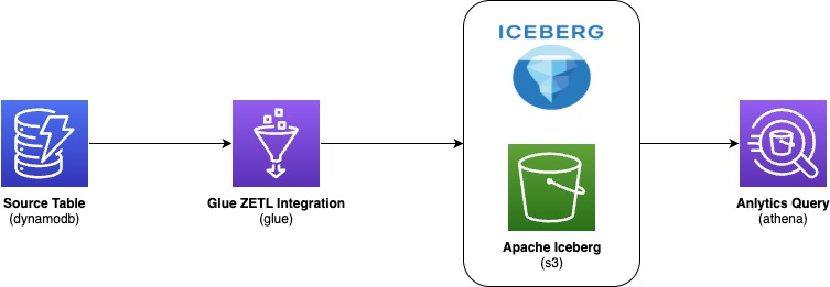
You replicate data from your DynamoDB table through AWS Glue Zero-ETL into Apache Iceberg tables stored in Amazon S3, then query the results with Amazon Athena. The following diagram illustrates the end-to-end architecture:

Data flow diagram showing AWS data pipeline: DynamoDB source table → AWS Glue zero-ETL integration → Apache Iceberg on Amazon S3 → Amazon Athena analytics query.

AWS Glue zero-ETL ingests data from Amazon DynamoDB, writes it in Apache Iceberg format to your Amazon S3 data lake, and makes it available for SQL queries in Amazon Athena—with no pipelines to build or maintain. With this integration, you:

  • Save development time by skipping custom code and ETL job management
  • Keep DynamoDB performance intact because replication doesn’t consume table’s provisioned read/write capacity
  • Get data within 15 minutes of changes in the source table
  • Query with standard tools because data lands in Apache Iceberg format, an open table format that AWS natively supports for high-performance analytics

During setup, you configure two output settings:

  1. Schema unnesting in Zero-ETL: You choose how nested attributes appear in the target. Flattening nested maps into individual columns streamlines your queries and reduces complexity.
  2. Data partitioning in Zero-ETL: You choose how data is organized into partitions. When you filter on a partition column, the query engine reads only matching data instead of scanning everything, cutting both query time and cost.

Schema unnesting

When you create a zero-ETL integration, you can choose one of three unnesting options. Schema unnesting transforms complex, nested DynamoDB structures into formats that analytics engines can query directly, removing post-processing transformations.

Each option changes how nested DynamoDB attributes appear in the target table. The right choice depends on your analytics tools and how consistent your DynamoDB schemas are.

Option 1: No unnesting

This option preserves the original nested structure. DynamoDB maps and lists remain as structured columns in the target.

Using the product example, the target table retains productid and value as columns to hold DynamoDB partition key and a DynamoDB record respectively.

Recommended for: Workloads where your analytics tools natively support querying nested data and you want to preserve the DynamoDB structure unchanged.

Option 2: Unnest one level

This option flattens top-level maps into individual columns. Lists remain nested.

With this option, productdetails and pricing each become separate columns.

Recommended for: Scenarios where your DynamoDB items have a consistent schema and you want to balance structure preservation with query simplicity.

Option 3: Unnest all levels (default)

This option recursively flattens nested structures using dot notation and produces the flattest schema.

For the product table, this creates columns such as productdetails.brand, productdetails.category, productdetails.specification.color , productdetails.specification.storage , pricing.list_price, and pricing.discount_pct. The pricing map flattens similarly. Each column is directly queryable without nested access patterns.

Recommended for: Analytics tools that prefer flat schemas when your DynamoDB items have a reasonably consistent structure. Note that deeply nested or highly variable schemas can produce very wide tables.

Data partitioning

You can speed up your queries and reduce costs by partitioning your replicated data. Partitioning divides data into logical segments on disk.

When you include a filter on a partition column in your query, the query engine skips irrelevant segments entirely. This behavior is called partition pruning: instead of scanning the entire dataset, the engine reads only the data that matches your filter conditions. For large tables, partition pruning can reduce both query runtime and cost significantly.

Default partitioning

If you don’t specify partition columns, AWS Glue Zero-ETL partitions data using the DynamoDB primary key with bucketing. This approach supports general-purpose queries without requiring manual configuration. For specific query patterns or performance requirements, you can define custom partitioning strategies described in the subsections that follow.

Identity partitioning

Identity partitioning uses raw column values to create partitions. You apply this strategy to low-to-medium cardinality columns such as brand, category, or AWS Region. To partition the product table by productdetails.brand and create a separate partition for each brand, use this configuration:

{
  "partitionSpec": [
    {
      "fieldName": "productdetails.brand",
      "functionSpec": "identity"
    }
  ]
}

With this setup, AWS Glue creates one partition directory per unique brand value. When you query for a specific brand, Athena reads only that partition.

Important: Avoid identity partitioning on high-cardinality columns such as primary keys or timestamps. This creates many small partitions, which degrades both ingestion and query performance

Time-based partitioning

Time-based partitioning organizes data by timestamp at a chosen granularity: year, month, day, or hour. You apply this strategy to time-series data and time-range queries. To partition the product table by month on the created_at column, which stores epoch milliseconds, use this configuration:

{
  "partitionSpec": [
    {
      "fieldName": "created_at",
      "functionSpec": "month",
      "conversionSpec": "epoch_milli"
    }
  ]
}

The conversionSpec parameter tells AWS Glue how to interpret the source timestamp. Supported values: epoch_sec (Unix seconds), epoch_milli (Unix milliseconds), and iso (ISO 8601 format).

Note: The original column values remain unchanged. AWS Glue transforms only the partition column values to timestamp type in the target table

Multi-level partitioning

You can combine strategies for a hierarchical scheme. To partition first by month and then by brand, use this configuration:

{
  "partitionSpec": [
    {
      "fieldName": "created_at",
      "functionSpec": "month",
      "conversionSpec": "epoch_milli"
    },
    {
      "fieldName": "productdetails.brand",
      "functionSpec": "identity"
    }
  ]
}

This scheme supports efficient queries that filter by date range, brand, or both. Place higher-selectivity columns first in the hierarchy and align the scheme with your most common query patterns.

Best practices

Keep these guidelines in mind when you configure your integration:

  • Avoid identity partitioning on high-cardinality columns such as primary keys, timestamps, or system-generated IDs. This leads to partition explosion and degrades performance.
  • Apply only one time-based function per column. For example, don’t partition col1 by year, month, day, and hour simultaneously.
  • Match conversionSpec to your actual data format. If your timestamps are in epoch milliseconds, use epoch_milli, not epoch_sec or iso.
  • Choose granularity based on data volume. High-volume tables benefit from finer granularity (day or hour). Lower-volume tables work well with coarser granularity (month or year).
  • Account for timezone implications with ISO timestamps. AWS Glue Zero-ETL normalizes timestamp partition values to UTC.

Prerequisites

To implement the AWS Glue Zero-ETL integration with a DynamoDB source, you will need:

  1. An AWS account with least privilege principle
  2. An AWS Glue database (for example, ddb_zero_etl_demo_db) with an Amazon S3 bucket associated as the database location (setup instructions)
  3. AWS Glue Data Catalog settings updated with an AWS Identity and Access Management (IAM) policy that grants fine-grained access control for zero-ETL (setup instructions)
  4. Create an IAM role named zetl-role, to be used by zero-ETL to access data from your DynamoDB table
  5. A DynamoDB source table (for example, product) configured for zero-ETL integration (setup instructions)

Walkthrough: Create the zero-ETL integration

Complete these steps to create a zero-ETL integration with DynamoDB as the source and Apache Iceberg tables in Amazon S3 as the target.

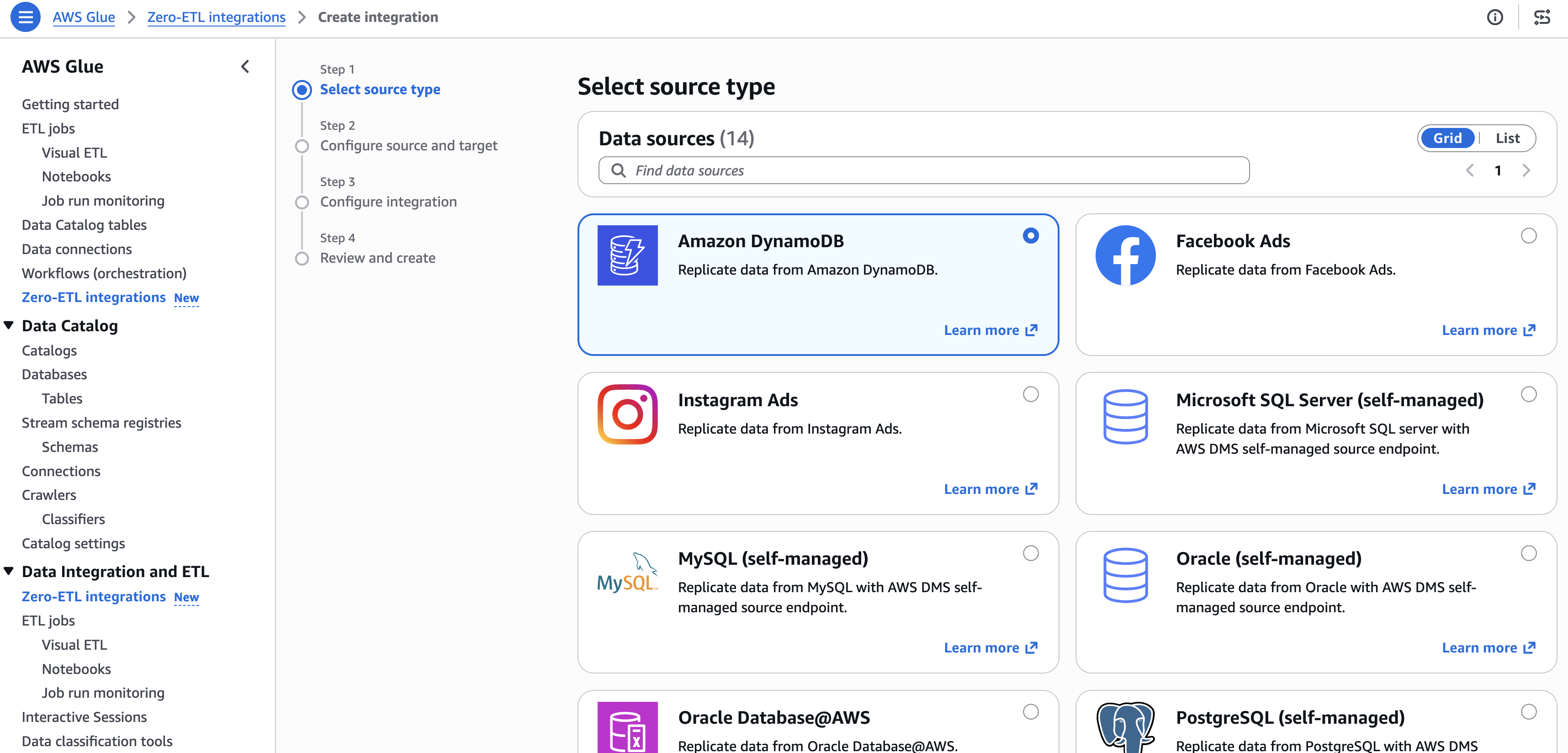
Step 1: Select the source type

  1. Open the AWS Glue console.
  2. In the navigation pane, under Data Integration and ETL, choose Zero-ETL integrations.
  3. Choose Create zero-ETL integration.
  4. Select Amazon DynamoDB as the source type, then choose Next.

AWS Glue console showing Step 1 of creating a Zero-ETL integration — selecting a source type from 14 available data sources including Amazon DynamoDB, Facebook Ads, Instagram Ads, MySQL, Oracle, PostgreSQL, and Microsoft SQL Server

[Figure 1: Selecting Amazon DynamoDB as the zero-ETL source type]

Step 2: Configure source and target

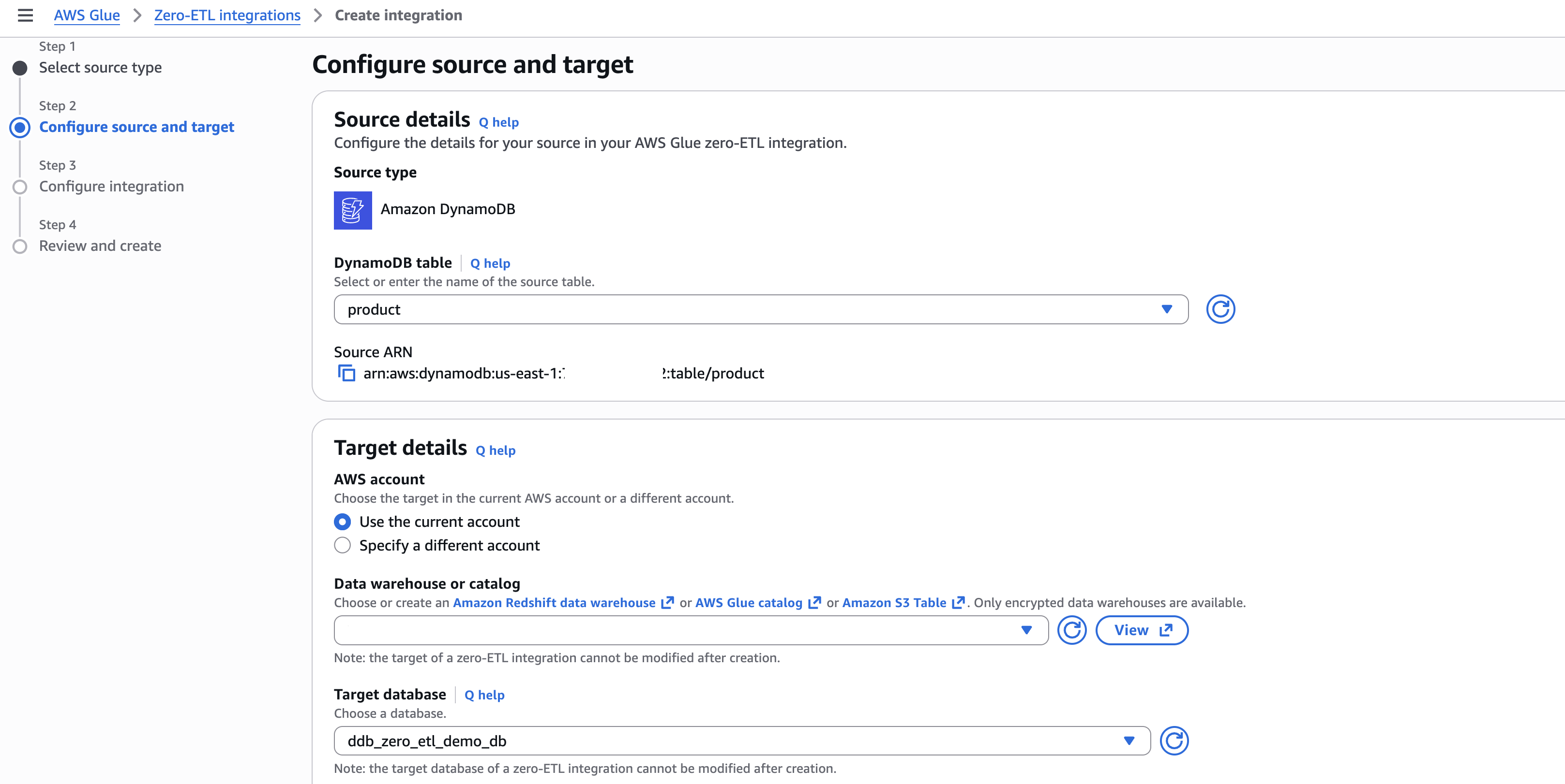
  1. In Source details, select your DynamoDB table (for example, product).
  2. In Target details:
    • Select the current account as target.
    • Choose the catalog and target database (for example, ddb_zero_etl_demo_db).
    • Select the IAM role (for example, zetl-role).

AWS Glue console Step 2 — configuring source and target for a zero-ETL integration with Amazon DynamoDB "product" table as source and an AWS Glue catalog database "ddb_zero_etl_demo_db" as target

[Figure 2: Configuring source DynamoDB table and target database]

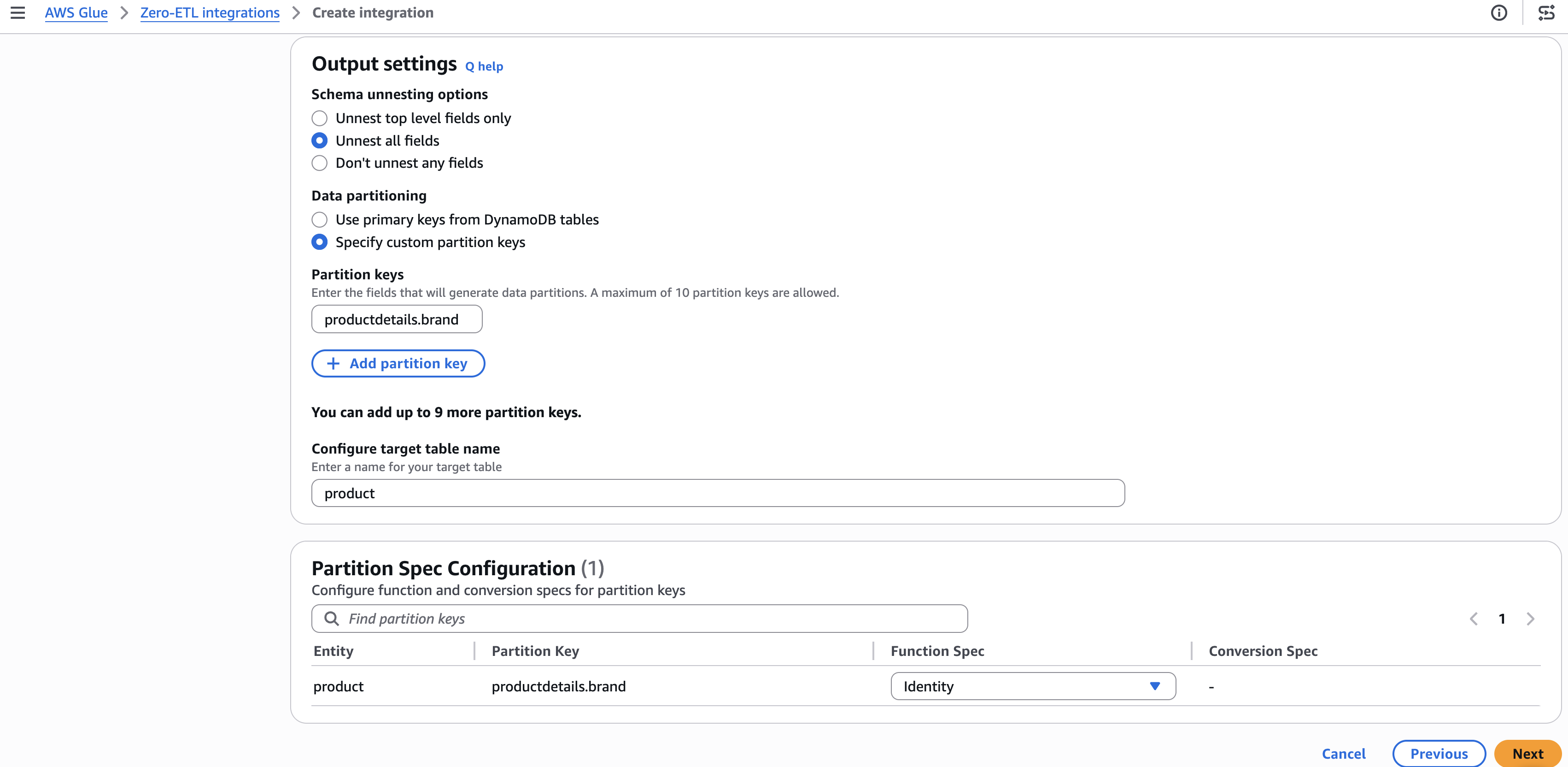
Step 3: Configure output settings

  1. Under Schema unnesting, select Unnest all fields.
  2. Under Data partitioning, select Specify custom partition keys.
  3. Enter the partition key (for example, productdetails.brand) and set the function to Identity.
  4. Choose Next.

AWS Glue Zero-ETL integration output settings showing schema unnesting set to "Unnest all fields," custom partition key "productdetails.brand" configured with Identity function, and target table named "product.

[Figure 3: Configuring schema unnesting and partition key settings]

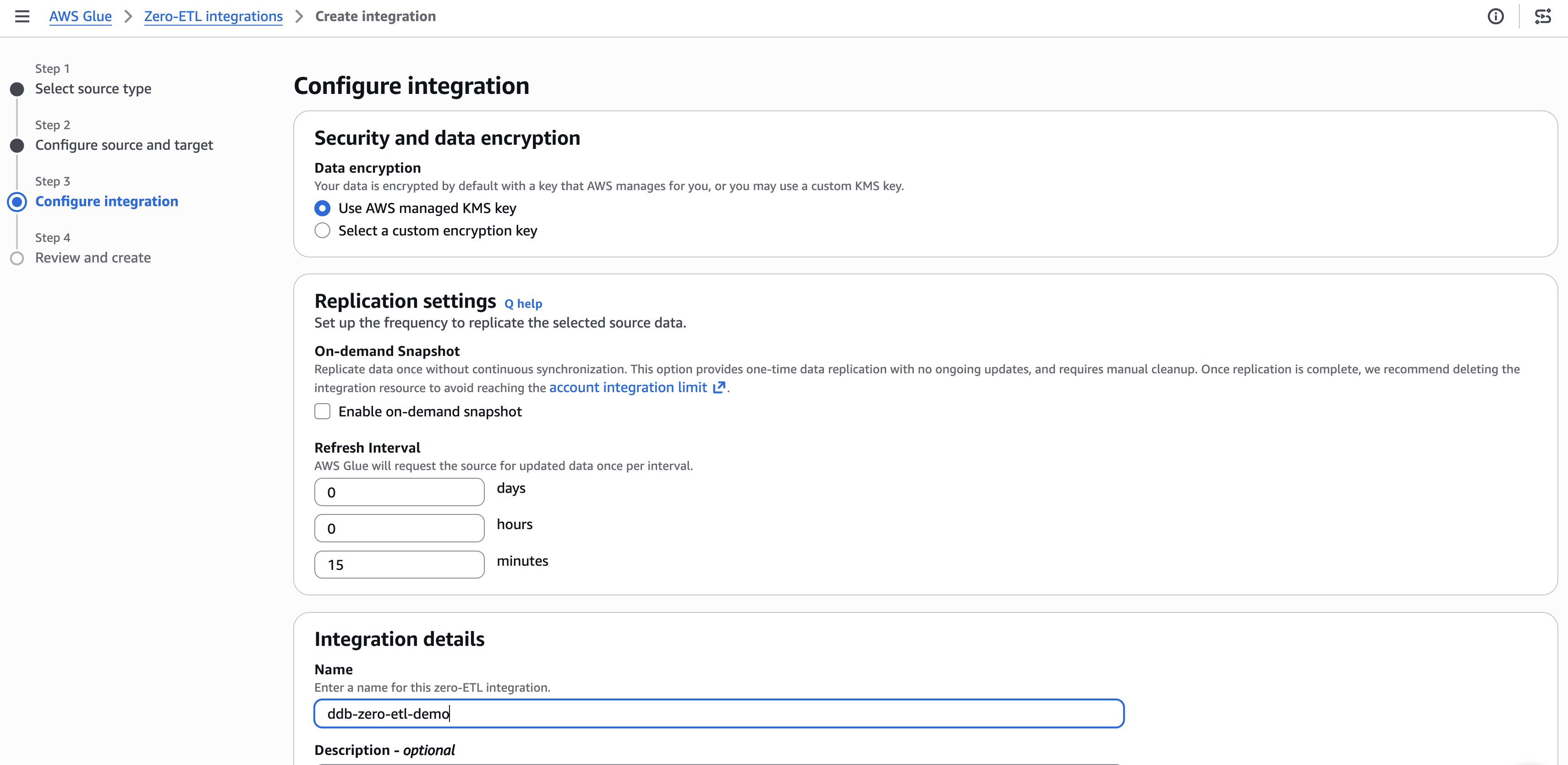
Step 4: Set integration details

  1. Optionally configure encryption and replication settings. The default refresh interval is 15 minutes.
  2. Enter a name for the integration (for example, ddb-zero-etl-demo).
  3. Choose Next.

AWS Glue Zero-ETL integration Step 3 — configuring security with AWS managed KMS key, replication refresh interval set to 15 minutes, and integration named "ddb-zero-etl-demd

[Figure 4: Configuring encryption and replication settings]

Step 5: Review and create

  1. Review your settings and choose Create and launch integration.
  2. The integration shows as Active within about a minute.

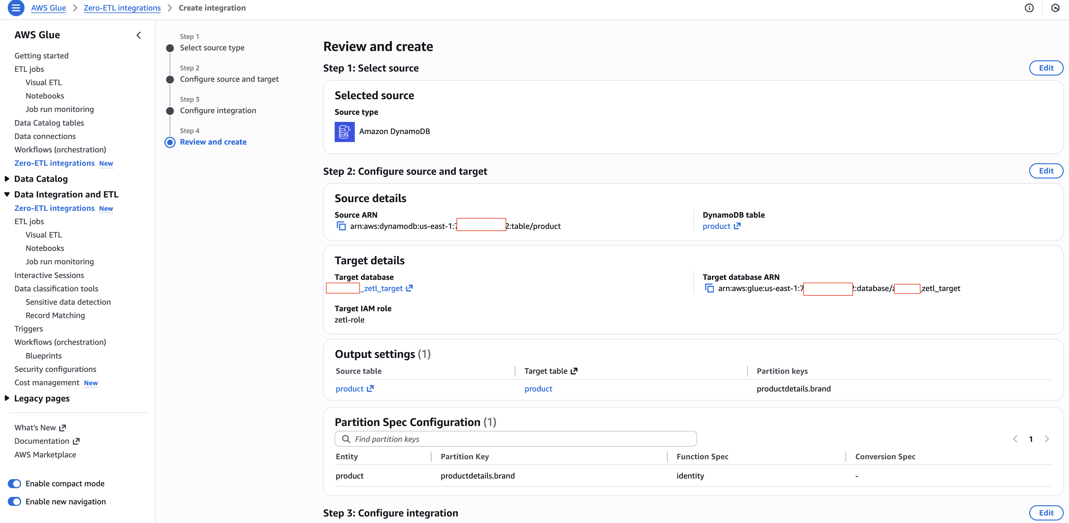
AWS Glue Zero-ETL integration Step 4: Review and Create — showing DynamoDB "product" table as source, Glue database "zett_target" as target with IAM role "zett-role," and partition key "productdetails.brand" with Identity function

[Figure 5: Review and create summary]

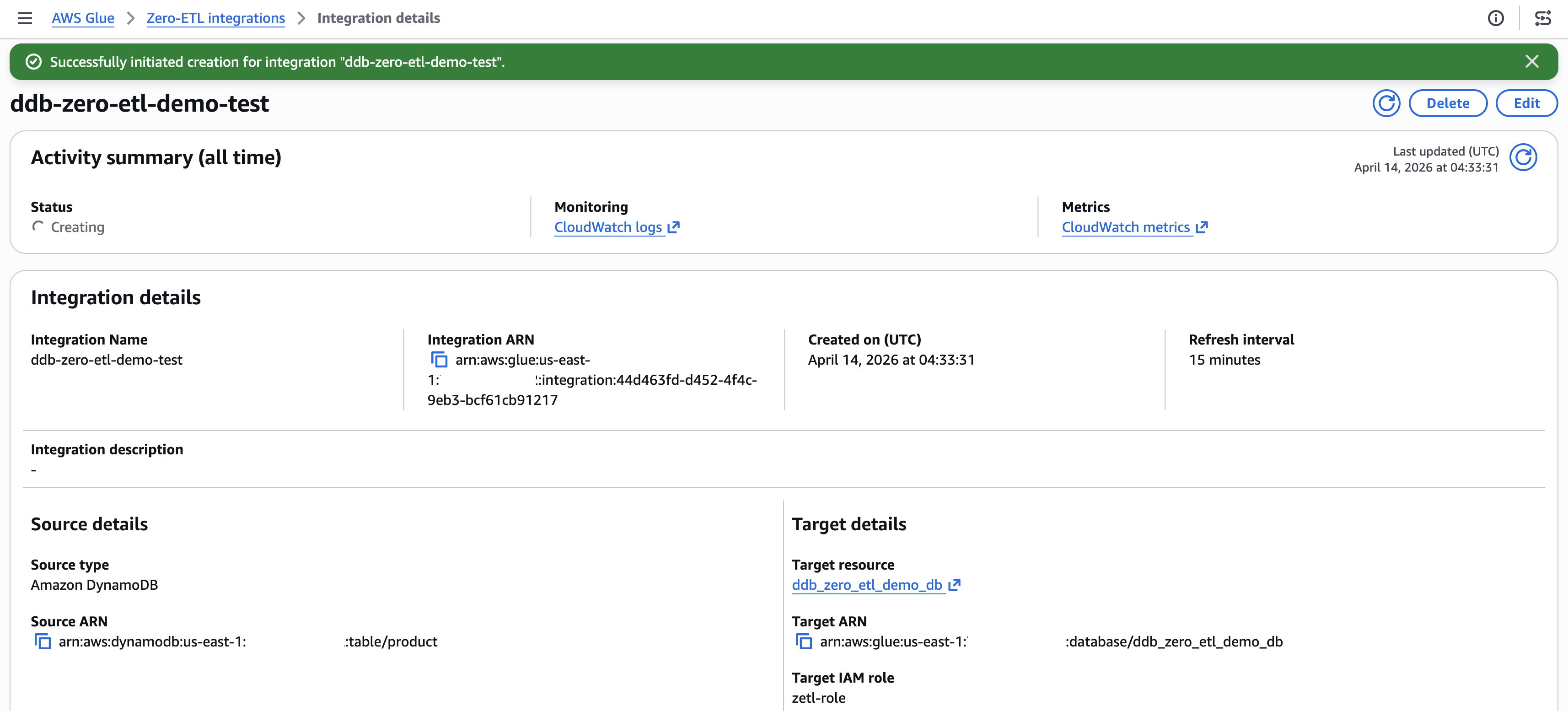
AWS Glue Zero-ETL Integration Details page showing "ddb-zero-etl-demo-test" integration with status "Creating," DynamoDB "product" table as source, Glue database "ddb_zero_etl_demo_db" as target, and a 15-minute refresh interval

[Figure 6: Integration active with successful status]

Query the replicated data

After the integration is active and the initial replication completes (typically 15–30 minutes), you can query the data in Amazon Athena.

Preview the replicated data

  1. Open the Amazon Athena console.
  2. In the query editor, select your target database (for example, ddb_zero_etl_demo_db).
  3. Run a preview query:
SELECT * FROM "ddb_zero_etl_demo_db"."product"LIMIT 10;

Verify schema unnesting

With Unnest all fields selected, nested attributes appear as individual columns with dot notation:

SELECT "productdetails.brand", "productdetails.category", "pricing.list_price" 
FROM "ddb_zero_etl_demo_db"."product"
WHERE "productdetails.category" = 'Electronics';

Verify partition pruning

Queries that filter on the partition column (productdetails.brand) automatically skip irrelevant partitions:

SELECT product_id, name, "pricing.list_price"
FROM "ddb_zero_etl_demo_db"."product"
WHERE "productdetails.brand" = 'AudioTech';

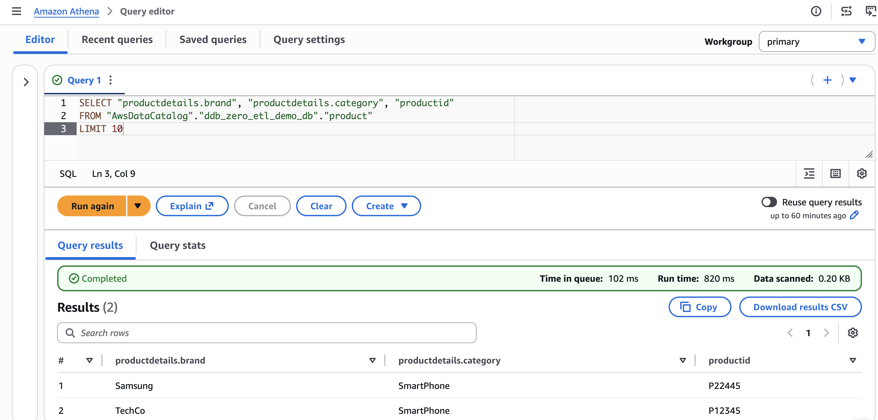
Amazon Athena Query Editor showing a completed SQL query selecting brand, category, and product ID from a DynamoDB zero-ETL Glue catalog table, returning two results: Samsung SmartPhone P22445 and TechCo SmartPhone P12345

[Figure 7: Athena query to retrieve the data from Apache Iceberg lakehouse]

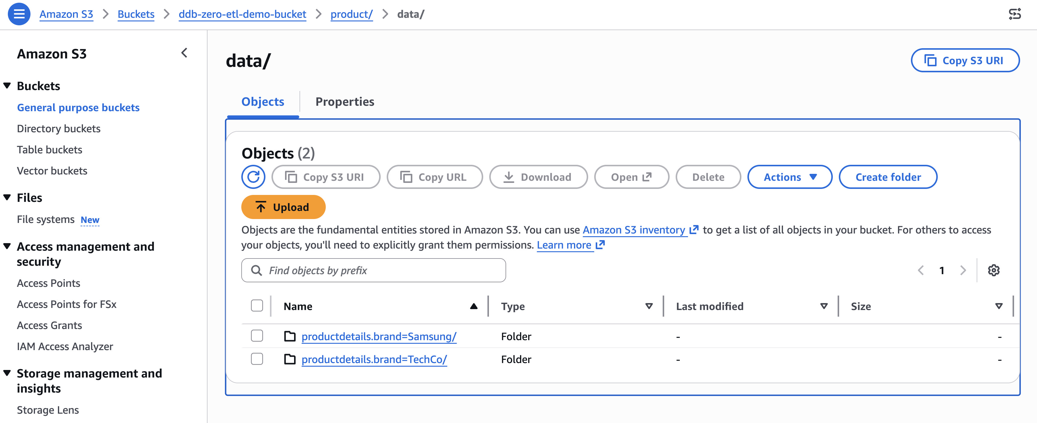
You can verify the partition structure by navigating to the Amazon S3 bucket associated with your database. The data organizes into directories like:

Amazon S3 bucket browser showing the "data/" folder in "ddb-zero-etl-demo-bucket" with two partitioned folders: "productdetails.brand=Samsung/" and "productdetails.brand=TechCo/" — confirming Iceberg partition structure from DynamoDB zero-ETL integration

[Figure 8: Amazon S3 bucket organization for the identity partition productdetails.brand]

Clean up

To avoid ongoing charges, delete the resources in this order:

  1. Delete the zero-ETL integration. In the AWS Glue console, navigate to Zero-ETL integrations, select your integration, and choose Delete. Existing replicated data remains in the target, but new changes stop replicating.
  2. Delete the replicated table. In the AWS Glue Data Catalog, navigate to Tables, select the replicated table, and delete it.
  3. Delete the AWS Glue database. In the Data Catalog, select the database and delete it.
  4. Delete the Amazon S3 data. Empty and delete the S3 bucket associated with the database.
  5. Delete the DynamoDB table. If you created it for this walkthrough, delete the source table.
  6. Delete IAM resources. Remove the IAM role and policies created for the integration.

Conclusion

You configured schema unnesting and data partitioning for a DynamoDB zero-ETL integration, replicated a product catalog table to Apache Iceberg tables in Amazon S3, and verified the results in Amazon Athena. Unnesting flattened nested attributes into directly queryable columns. Partitioning helped the query engine skip irrelevant data, reducing both query time and cost. To take your integration further, try monitoring replication lag and data freshness with Amazon CloudWatch metrics. You can also experiment with different partitioning strategies on a staging table before applying them to production workloads, testing time-based partitioning alongside identity partitioning to find the optimal scheme for your query patterns. For broader analytics coverage, query the same Iceberg tables from Amazon Redshift Spectrum or Amazon EMR alongside Athena. For more details, explore these resources:


About the authors

Raju Ansari

Raju is a Senior Software Development Engineer at AWS, specializing in building scalable, secure, serverless solutions that simplify data analytics and AI agent development. He helps organizations modernize their data analytics infrastructure and develop cutting-edge AI agentic applications. Currently, Raju focuses on building foundational AI services, including Amazon Bedrock Agents, which enable developers to create intelligent, autonomous applications at scale. Outside of work, Raju is passionate about giving back to the tech community. He actively volunteers at IEEE events and mentor early and mid-career professionals

Shashank Sharma

Shashank is an Engineering Leader with over 15 years of experience delivering data integration and replication solutions for first-party and third-party databases and SaaS for enterprise customers. He leads engineering for AWS Glue Zero-ETL and Amazon AppFlow, building fully managed pipelines that replicate data from sources like Salesforce, SAP, DynamoDB, and Oracle into Amazon Redshift and Apache Iceberg-based data lakes. Shashank advises startups on technology strategy and mentors engineers and technical leaders at various career stages

Implement a data mesh pattern in Amazon SageMaker Catalog without changing applications

Post Syndicated from Paolo Romagnoli original https://aws.amazon.com/blogs/big-data/implement-a-data-mesh-pattern-with-amazon-sagemaker-catalog-without-making-changes-to-your-applications/

When creating a project in Amazon SageMaker Unified Studio, users select a project profile to define resources and tools to be provisioned in the project. These are used by Amazon SageMaker Catalog to implement a data mesh pattern. Some users don’t want to take advantage of resources provisioned along with the project for various reasons. For instance, they may want to avoid making changes to their existing applications and data products.

This post shows you how to implement a data mesh pattern by using Amazon SageMaker Catalog while keeping your current data repositories and consumer applications unchanged.

Solution overview

In this post, you will simulate a scenario based on data producer and data consumer that exists before Amazon SageMaker Catalog adoption. For this purpose, you will use a sample dataset to simulate existing data and simulate an existing application using an AWS Lambda function. You can apply the same solution to your real-life data and workloads.

The following diagram illustrates the solution architecture’s key configurations. In this architecture, the Amazon Simple Storage Service (Amazon S3) bucket and the AWS Glue Data Catalog in the producer account simulate the existing data repository. The Lambda function in the consumer account simulates the existing consumer application.

AWS cross-account data sharing via SageMaker & Lake Formation: Producer publishes to catalog, Consumer subscribes & accesses data

Here is a description of the key configurations highlighted in the architecture:

  1. As part of an Amazon SageMaker domain, create a producer project (associated to a producer account) and a consumer project (associated to a consumer account). Among other resources, a project AWS Identity and Access Management (IAM) role is created for each project in the associated account.
  2. In the producer account, use AWS Lake Formation to grant producer project’s IAM role permissions to access the existing data asset.
  3. Publish the data asset in the Amazon SageMaker Catalog from the producer project.
  4. Subscribe the data asset from the consumer project.
  5. In the consumer account, configure your Lambda function to assume consumer project’s IAM role to access the subscribed data asset.

The solution architecture is based on the following Amazon Web Services (AWS) services and features:

  • Amazon SageMaker Catalog offers you a way to discover, govern, and collaborate on data and AI securely.
  • Amazon SageMaker Unified Studio provides a single data and AI development environment to discover and build with your data. Amazon SageMaker Unified Studio projects provide collaborative boundaries for users to accomplish data and AI tasks.
  • The lakehouse architecture of Amazon SageMaker is fully compatible with Apache Iceberg. It unifies data across Amazon S3 data lakes, Amazon Redshift data warehouses, and third-party and federated data sources.
  • AWS Lake Formation, which you can use centrally to govern, secure, and share data for analytics and machine learning.
  • AWS Glue Data Catalog is a persistent metadata store for your data assets. It contains table definitions, job definitions, schemas, and other control information to help you manage your AWS Glue environment.
  • Amazon S3 is an object storage service that offers industry-leading scalability, data availability, security, and performance.

Setting up resources

In this section, you will prepare the resources and configurations you need for this solution.

Three AWS accounts

To follow this solution, you need three AWS accounts, and it’s better if they’re part of the same organization in AWS Organizations:

  • Producer account – Hosts the data asset to be published
  • Consumer account – Hosts the application that consumes the data published from the producer account
  • Governance account – Where the Amazon SageMaker Unified Studio domain is configured

Each account must have an Amazon Virtual Private Cloud (Amazon VPC) with at least two private subnets in two different Availability Zones. For instruction, refer to Create a VPC plus other VPC resources. Make sure to create both VPCs in the same Region you plan to apply this solution.

A governance account is used for the sake of convenience, but it’s not strictly needed because Amazon SageMaker can be configured and managed in producer or consumer accounts.If you don’t have access to three accounts, you can still use this post to understand the key configurations required to implement a data mesh pattern with Amazon SageMaker Catalog while keeping your current data repositories and consumer applications unchanged.

Create a data repository in the producer account

First, create a sample dataset by following these instructions:

  1. Open a text editor.
  2. Paste the following text in a new file:
    name,stars
    	oak,3
    	maple,2
    	birch,3
    	willow,4
    	pine,5
    	mango,1
    	neem,2
    	banyan,5
    	eucalyptus,3
    	teak,2

  3. Save the file as trees.csv. This is your sample data file.

After you create the sample dataset, create an S3 bucket and an AWS Glue database in the producer account, which will act as the data repository.

Create the S3 bucket and upload the trees.csv file in the producer account:

  1. Access the S3 console in the producer account.
  2. Create an S3 bucket. For instructions, refer to Creating a general purpose bucket.
  3. Upload to the S3 bucket the trees.csv sample data file that you created. For instructions, refer to Uploading objects.

Create the AWS Glue database and table in the producer account:

  1. Access the Glue console in the producer account.
  2. In the navigation pane, under Data Catalog, choose Databases.
  3. Choose Add database.
  4. For Name, enter collections.
  5. For Description, enter This database contains collections of statistics for natural resources.
  6. Choose Create database.
  7. In the navigation pane, under Data Catalog, choose Tables.
  8. Choose Add table.
  9. In the table creation guided procedure, enter the following input for Step 1: Set table properties:
    1. For Name, enter trees.
    2. For Database, select collections.
    3. For Description, enter This table captures ratings data related to the characteristics of various tree species.
    4. For Table format, select Standard AWS Glue table (default).
    5. For Select the type of source, select S3.
    6. For Data location is specified in, select my account.
    7. For Include path, enter s3://<bucket-name>/<prefix>/ where <bucket-name> is the name of the S3 bucket you created earlier in this procedure and <prefix> is the optional prefix for the trees.csv file you uploaded.
    8. For Data format, select CSV.
    9. For Delimeter, select Comma (,).
  10. Choose Next.
  11. For Step 2: Choose or define schema, enter the following:
    1. For Schema, select Define or upload a schema.
    2. Choose Edit schema as JSON and enter the following schema in the pop-up:
      [
        {
          "Name": "name",
          "Type": "string",
          "Parameters": {}
        },
        {
          "Name": "stars",
          "Type": "string",
          "Parameters": {}
        }
      ]

    3. Choose Save.
    4. Choose Next.
    5. Choose Create.

Create a Lambda function in the consumer account

Create the Lambda function in the consumer account. This will simulate a data consumer application.First, in the consumer account create the IAM policy and the IAM role to be assigned to the Lambda function:

  1. Access the IAM console in the consumer account.
  2. Create an IAM policy and name it smus_consumer_athena_execution by using the following policy. Make sure to replace placeholders <AWS_Region> and <AWS_account_ID_number> with your Region and consumer account ID number. You will replace the <workgroup_id> placeholder later. For IAM policy creation instructions, refer to Create IAM policies (console).
    {
        "Version": "2012-10-17",
        "Statement": [
            {
                "Sid": "AthenaExecution",
                "Action": [
                    "athena:StartQueryExecution",
                    "athena:GetQueryExecution",
                    "athena:GetQueryResults"
                ],
                "Effect": "Allow",
                "Resource": "arn:aws:athena:<AWS_Region>:<AWS_account_ID_number>:workgroup/<workgroup_id>"
            }
        ]
    }

  3. Create an IAM role for AWS Lambda service and name it smus_consumer_lambda. Assign to it the AWS managed permission AWSLambdaBasicExecutionRole and the permission named smus_consumer_athena_execution that you just created. For instructions, refer to Create a role to delegate permissions to an AWS service.

After the IAM role for the Lambda function is in place, you can create the Lambda function in the consumer account:

  1. Access the Lambda console in the consumer account.
  2. In the navigation pane, choose Functions.
  3. Choose Create function and enter the following information:
    1. For Function name, enter consumer_function.
    2. For Runtime, select Python 3.14.
    3. Expand Change default execution role section.
    4. For Execution role, select Use an existing role.
    5. For Existing role, select smus_consumer_lambda.
  4. Choose Create function.
  5. Under the Code tab, in the Code source, replace the existing code with the following:
    import boto3
    import time
    sts_client = boto3.client('sts')
    role_arn = "<role_arn>"
    session_name = "AthenaQuerySession"
    catalog = "AwsDataCatalog"
    database = "<database_name>"
    workgroup = "<workgroup_id>"
    query = "select * from "+catalog+"."+database+".trees"
    def lambda_handler(event, context):
        # Assume SageMaker Unified Studio project role
        assumed_role_object = sts_client.assume_role(
            RoleArn=role_arn,
            RoleSessionName=session_name
        )
        # Get temporary credentials
        credentials = assumed_role_object['Credentials']
        # Create Athena client using temporary credentials
        athena = boto3.client(
            'athena',
            aws_access_key_id=credentials['AccessKeyId'],
            aws_secret_access_key=credentials['SecretAccessKey'],
            aws_session_token=credentials['SessionToken'],
            region_name='eu-west-1'
        )
        # Execute Athena Query
        response = athena.start_query_execution(
            QueryString=query,
            QueryExecutionContext={
                'Database': database,
                'Catalog': catalog
            },
            WorkGroup=workgroup
        )
        query_execution_id = response['QueryExecutionId']
        # Polling with exponential backoff
        wait_time = 0.25  # Start with 0.25 seconds
        max_wait = 8      # Maximum wait time of 8 seconds
        
        while True:
            result = athena.get_query_execution(QueryExecutionId=query_execution_id)
            state = result['QueryExecution']['Status']['State']
            if state in ['FAILED', 'CANCELLED']:
                raise Exception(f"Query {state}")
            elif state == 'SUCCEEDED':
                break
            elif state in ['QUEUED', 'RUNNING']:
                time.sleep(wait_time)
                wait_time = min(wait_time * 2, max_wait)  # Double wait time, cap at max_wait
        # Retrieve results
        results = athena.get_query_results(QueryExecutionId=query_execution_id)
        return results

  6. Choose Deploy.

The code provided for the Lambda function includes some placeholders that you will replace later, after you have the required information. Don’t test the Lambda function at this time because it will fail because of the presence of the placeholders.

Create a user with administrative access

Amazon SageMaker Unified Studio supports two distinct domain types: AWS IAM Identity Center based domains and IAM based domains. At the time of writing this post, only IAM Identity Center based domains support multi-accounts association, therefore in this post you work with this type of domain that requires IAM Identity Center.

In the governance account, you enable IAM Identity Center and create an administrative user to create and manage the Amazon SageMaker Unified Studio domain. Create a user with administrative access:

  1. Enable IAM Identity Center in the governance account. For instructions, refer to Enable IAM Identity Center.
  2. In IAM Identity Center in the governance account, grant administrative access to a user. For a tutorial about using the IAM Identity Center directory as your identity source, refer to Configure user access with the default IAM Identity Center directory.

Sign in as the user with administrative access:

  • To sign in with your IAM Identity Center user, use the sign-in URL that was sent to your email address when you created the IAM Identity Center user. For help signing in using an IAM Identity Center user, refer to Sign in to your AWS access portal.

Create a SageMaker Unified Studio domain

To create the Amazon SageMaker Unified Studio domain in the governance account refer to Create a Amazon SageMaker Unified Studio domain – quick setup.

After your domain is created, you can navigate to the Amazon SageMaker Unified Studio portal (a browser-based web application) where you can use your data and configured tools for analytics and AI. Save the Amazon SageMaker Unified Studio portal URL because you will use this URL later.

Solution steps

Now that you have the prerequisites in place, you can complete the following ten high-level steps to implement the solution.

Associate the producer and consumer accounts to the Amazon SageMaker Unified Studio domain

Start by associating the producer and consumer accounts to the newly created Amazon SageMaker Unified Studio domain. When you associate your producer and consumer accounts to the domain, make sure to select IAM users and roles can access APIs and IAM users can log in to Amazon SageMaker Unified Studio in the AWS RAM share managed permission section. For step-by-step instructions, refer to Associated accounts in Amazon SageMaker Unified Studio. If your AWS accounts are part of the same organization, your association requests are automatically accepted. However, if your AWS accounts aren’t part of the same organization, request association with the other AWS accounts in the governance account and then accept the association request in both the producer and consumer accounts.

Create two project profiles

Now, create two project profiles, one for the producer project and one for the consumer project.

In Amazon SageMaker Unified Studio, a project profile defines an uber template for projects in your Amazon SageMaker domain. A project profile is a collection of blueprints that provides reusable AWS CloudFormation templates used to create project resources.

A project profile is associated to a specific AWS account. This means, when a project is created the blueprints listed in the project profile are deployed in the associated AWS account. To use a project profile, you must enable its blueprints in the AWS account associated to the project profile.

Create the producer project profile

You’re going to create the producer project profile that is associated to the producer account. This project profile will be used to create the producer project. This profile includes by default the Tooling blueprint that creates resources for the project, including IAM user roles and security groups.

Before creating the project profile, you will enable the Tooling blueprint in the producer account using the following procedure:

  1. Access the SageMaker console in the producer account.
  2. In the navigation pane, choose Associated domains.
  3. Select the domain you created while setting up.
  4. On the Blueprints tab, choose Enable in the Tooling blueprint section as shown in the following image:
  5. SageMaker Unified Studios Tooling blueprint config: disabled status with Enable button for IAM roles & AWS resource setup

  6. For Virtual private cloud (VPC) select your account VPC.
  7. For Subnets, select at least two subnets in different Availability Zones.
  8. Choose Enable blueprint.

Proceed to creating the project profile in the governance account:

  1. Access the SageMaker console in the governance account.
  2. In the navigation pane, choose Domains.
  3. Select the domain you created as part of prerequisites.
  4. Under the Project profiles tab, choose Create and enter the following information:
    1. For Project profile name, enter producer-project-profile.
    2. For Project profile creation options, select Custom create.
    3. DO NOT SELECT A BLUEPRINT for Blueprints because the Tooling blueprint is included by default in any project profile.
    4. For Account, select Provide an account ID.
    5. For Account ID, enter the producer account ID.
    6. For Region, select Provide region name and then select the Region in which you’re working.
    7. For Authorization, select Allow all users and groups.
    8. For Project profile readiness, select Enable project profile on creation.
  5. Choose Create project profile.

Create a consumer project profile

You also create a consumer project profile and associate it to the consumer account. This profile will be used to create the consumer project. The consumer project profile includes the LakeHouseDatabase blueprint, which is needed to create a lakehouse environment with an AWS Glue database for data management and an Amazon Athena workgroup for querying. The Tooling blueprint is included by default in the project profile.

Before creating the project profile, enable the Tooling and LakeHouseDatabase blueprints in the consumer account:

  1. Access the SageMaker console in the consumer account.
  2. In the navigation pane, choose Associated domains.
  3. Select the domain you created as part of prerequisites.
  4. On the Blueprints tab, choose Enable in the Tooling blueprint section.
  5. For Virtual private cloud (VPC) select your account VPC.
  6. For Subnets, select at least two subnets in different Availability Zones.
  7. Choose Enable blueprint.
  8. In the navigation pane, choose Associated domains.
  9. Select the domain you created as part of prerequisites.
  10. Under the Blueprints tab, select the LakeHouseDatabase blueprint.
  11. Choose Enable.
  12. Choose Enable blueprint.

After blueprints are enabled in the consumer account, you can proceed creating the project profile:

  1. Access the SageMaker console in the governance account.
  2. In the navigation pane, choose Domains.
  3. Select the domain you created as part of prerequisites.
  4. Under Project profiles tab choose Create and enter the following information:
    1. For Project profile name, enter consumer-project-profile.
    2. For Project profile creation options, select Custom create.
    3. For Blueprints, select LakeHouseDatabase.
    4. For Account, select Provide an account ID.
    5. For Account ID, enter the consumer account ID.
    6. For Region, select Provide region name and then select the Region you are working.
    7. For Authorization, select Allow all users and groups.
    8. For Project profile readiness, select Enable project profile on creation.
  5. Choose Create project profile.

Create SageMaker Unified Studio producer and consumer projects

In Amazon SageMaker Unified Studio, a project is a boundary within a domain where you can collaborate with other users to work on a business use case. In projects, you can create and share data and resources.To create producer and consumer projects in Amazon SageMaker Unified Studio use the following instructions:

  1. Access the Amazon SageMaker Unified Studio portal.
  2. Choose the Select a project dropdown list.
  3. Choose Create project and enter the following information:
    1. For Project name, enter Producer.
    2. For Project profile, select producer-project-profile.
  4. Choose Continue.
  5. Choose Continue.
  6. Choose Create project.

After you’ve created the Producer project, note in a text file the Project role ARN that is displayed in the Project overview. The following image is shown for reference. The project role name is the string that follows arn:aws:iam::<account_ID>:role/ in the project role Amazon Resource Name (ARN). You will use both project role name and ARN later.

SageMaker Producer project overview: active status, files listed, S3 location & IAM role ARN displayed in project details tab

Repeat the preceding procedure to create the Consumer project. Be sure to enter Consumer for Project name and then select consumer-project-profile for Project profile. After it’s created, note the Project role ARN in a text file. The project role name is the string that follows arn:aws:iam::<account_ID>:role/ in the project role ARN. You will use both project role name and ARN later.

Bring your own data from the producer account

Bring your own data to the Amazon SageMaker Unified Studio Producer project. AWS provides several options to achieve this onboarding. The first option is automated onboarding in Amazon SageMaker lakehouse, in which you ingest the Amazon SageMaker lakehouse metadata of datasets into Amazon SageMaker Catalog. With this option, you can onboard your Amazon SageMaker lakehouse data as part of creating a new Amazon SageMaker Unified Studio domain or for an existing domain.

For more information about automated onboarding of Amazon SageMaker lakehouse data, refer to Onboarding data in Amazon SageMaker Unified Studio. As other options, you can bring in existing resources to your Amazon SageMaker Unified Studio project by using the Data and Compute pages in your project, or by using scripts provided in GitHub. For more information about using the Data and Compute pages or about using scripts, refer to Bringing existing resources into Amazon SageMaker Unified Studio. In this post, you will use Amazon SageMaker lakehouse capabilities to import your trees AWS Glue table into the Producer project.

Register the Amazon S3 location for the table

To use Lake Formation permissions for fine-grained access control to the trees table, you need to register in Lake Formation the Amazon S3 location of the trees table. To do that, complete the following actions:

  1. Access the Lake Formation console in the producer account.
  2. In the navigation pane under Administration, choose Data lake locations.
  3. Choose Register location and enter the following information:
    1. For S3 URI, enter s3://<bucket-name>/<prefix>/ where <bucket-name> is the name of the S3 bucket you created in the prerequisites and <prefix> is the optional prefix for the trees.csv file you uploaded as part of the prerequisite.
    2. For IAM role, select AWSServiceRoleForLakeFormationDataAccess.
    3. For Permission mode, select Lake Formation.
  4. Choose Register location.

Grant Producer project role permissions on the database

Grant database access to the IAM role that is associated with your Producer project. This role is called the project role, and it was created in IAM upon project creation.

To access the AWS Glue Data Catalog collections database from the Producer project in the Amazon SageMaker Unified Studio, complete the following actions:

  1. Access the Lake Formation console in the producer account.
  2. In the navigation pane under Data Catalog, choose Databases.
  3. Choose the collections database.
  4. From the Actions menu, choose Grant and enter the following information:
    1. For IAM users and roles, select your Producer project’s role name. This is the string starting with datazone_usr_role_ that is part of the Producer project role ARN that you noted in step 3 “Create SageMaker Unified Studio producer and consumer projects”.
    2. For Database permissions, select Describe.
  5. Choose Grant.

Grant Producer project role permissions on the table

Grant trees table access to the IAM role that is associated with your Producer project. To grant these permissions use the following instructions:

  1. Access the Lake Formation console in the producer account.
  2. In the navigation pane under Data Catalog, choose Tables and MVs.
  3. Select the trees table.
  4. From the Actions menu, choose Grant and enter the following information:
    1. For IAM users and roles, select your Producer project’s role. This is the string starting with datazone_usr_role_ that is part of the Producerproject role ARN that you noted in step 3 “Create SageMaker Unified Studio producer and consumer projects”.
    2. For Table permissions, select Select and Describe.
    3. For Grantable permissions, select Select and Describe.
  5. Choose Grant.

Revoke any existing permissions of IAMAllowedPrincipals

You must revoke the IAMAllowedPrincipals group permissions on both the database and table to enforce Lake Formation permission for access. For more information, refer to Revoking permission using the Lake Formation console.

  1. Access the Lake Formation console in the producer account.
  2. In the navigation pane under Permission, choose Data permissions.
  3. Select the entries where Principal is set to IAMAllowedPrincipals and Resource is set to collections or trees as in the following image:
  4. Data permissions table: 2 of 5 IAMAllowedPrincipals entries selected. All permissions granted for collections DB & trees table

  5. Choose Revoke.
  6. Enter revoke.
  7. Choose Revoke again.

Verify that data is available in the Producer project

Verify that your collections database and trees table are accessible in the Producer project:

  1. Access the Amazon SageMaker Unified Studio portal.
  2. Choose the Select a project drop-down menu and choose the Producer project.
  3. In the navigation pane under Overview, choose Data.
  4. Choose Lakehouse.
  5. Choose AwsDataCatalog.
  6. Choose collections.
  7. Choose tables.
  8. Choose the three-dot action menu next to your trees table and choose Preview data, as shown in the following image.
    AWS Data Catalog interface: collections database in Lakehouse with trees table, presenting preview/notebook/drop options
  9. You’ll find data from the trees table as shown in the following image.
    Query Editor showing SQL query on trees table with results: oak (3 stars), maple (2), birch (3). Red arrow highlights output

Create Amazon SageMaker Catalog asset

Even if it’s accessible in the project, to work with the trees table in Amazon SageMaker Catalog, you need to register the data source and create an Amazon SageMaker Catalog asset:

  1. Access the Amazon SageMaker Unified Studio portal.
  2. Choose the Select a project dropdown list and choose the Producer project.
  3. On the project page, under Project catalog in the navigation pane, choose Data sources.
  4. Choose Create Data Source and make the following selections:
    1. For Name, enter collections.
    2. For Data source type, select AWS Glue (Lakehouse).
    3. For Database name, select collections.
    4. Choose Next.
    5. Choose Next.
    6. Choose Next.
    7. Choose Create.
  5. After the data source is created, you will be in the collections data source page, choose Run. This will import metadata and create the Amazon SageMaker Catalog asset.
  6. In the collections data source, on the Data source runs tab, you’ll find your run marked as Completed and the trees asset Successfully created, as shown in the following image:
    Producer project Assets page: Inventory tab presenting trees Glue Table asset with red arrows highlighting navigation & selection

Publish the data asset in the Amazon SageMaker Catalog

Publishing a data asset manually is a one-time operation that you need to perform to allow others to access the data asset through the catalog:

  1. Access the Amazon SageMaker Unified Studio portal.
  2. Choose the Select a project dropdown list and choose the Producer project.
  3. On the project page under Project catalog, choose Assets.
  4. Select your trees data asset that is available on the Inventory tab. The following image is shown for reference.
    Assets Inventory page: trees Glue Table listed in Producer project with navigation arrows highlighting menu selection
  5. (Optional) If automated metadata generation is enabled when the data source is created, metadata for assets (such as the asset business name) is available to review and accept or reject. You can either choose Accept All or Reject All in the Automated Metadata Generation banner.
  6. Choose Publish Asset. The following image is shown for reference.
    Asset overview: Agricultural Crop Yield dataset with automated metadata banner, ACCEPT ALL & PUBLISH ASSET buttons highlighted
  7. Choose Publish Asset.

Subscribe to the data asset in the Amazon SageMaker Catalog

To consume data assets in the Consumer project, subscribe to the data asset by creating a subscription request:

  1. Access the Amazon SageMaker Unified Studio portal.
  2. Choose the Select a project dropdown list and choose Consumer project.
  3. On the Discover menu, choose Catalog.
  4. Enter trees in the search box and then select the data asset returned from the search. If in step 7 “Publish the data asset in the Amazon SageMaker Catalog” you chose Accept All in the Automated Metadata Generation banner, your data asset will have a different business name generated by the automated metadata recommendations feature. The data asset technical name is trees. For reference, refer to the following image.
    Data Catalog search: 'trees' query shows Agricultural Crop Yield dataset with browse assets & data products options
  5. Choose Subscribe.
  6. For Comment, enter a justification such as This data asset is needed for model training purposes.
  7. Choose Subscribe again.

By default, asset subscription requests require manual approval by a data owner. However, if the requester in the Consumer project is also a member of the Producer project, the subscription request is automatically approved. For information about approving subscription requests, refer to Approve or reject a subscription request in Amazon SageMaker Unified Studio.

Configure your Lambda IAM role to access the subscribed data access

To enable your Lambda function access to the subscribed data asset, you need to allow the Lambda function to assume the Consumer project role. To do this, edit the Consumer project’s IAM role trust relationship:

  1. Navigate to the IAM console in the consumer account.
  2. In the navigation pane under Access management, choose Roles.
  3. Select the Consumer project’s IAM role. This is the string starting with datazone_usr_role_ that is part of the Consumer project role ARN that you noted in step 3 “Create SageMaker Unified Studio producer and consumer projects”.
  4. Under the Trust relationships tab, choose Edit trust policy.
  5. For backup reasons, make a copy of the existing trust policy in a text file.
  6. In the Edit trust policy window, add the following statement to the existing trust policy without removing or overwriting other existing statements in the trust policy. Be sure to replace the placeholder <account_id> with your consumer AWS account ID.
    {
        "Effect": "Allow",
        "Principal": {
            "AWS": "arn:aws:iam::<account_id>:role/smus_consumer_lambda"
        },
        "Action": [
            "sts:AssumeRole"
        ]
    }	

    IAM trust policy editor: JSON code with red arrow highlighting AWS principal ARN for smus_consumer_lambda role

  7. Choose Update policy.

Test the Lambda function’s access to the subscribed data asset

Before you can test your Lambda function, you need to replace placeholders in the function code and in the IAM policy. There are three placeholders to be replaced: <role_arn>, <database_name> and <workgroup_id>. For <role_arn>, you already have the actual value, which is the Consumer project’s role ARN that you noted in step 3 “Create SageMaker Unified Studio producer and consumer projects”. The next sections provide instructions to retrieve values for the other placeholders.

Retrieve the AWS Glue Data Catalog database name

You need to find the name of the AWS Glue Data Catalog database that was created along with the Consumer project. You will then use this value to replace the <database_name> placeholder in the consumer_function Lambda function code. To retrieve the AWS Glue Data Catalog database name, follow these instructions:

  1. Access the Amazon SageMaker Unified Studio portal.
  2. Choose the Select a project dropdown list and choose Consumer project.
  3. On the project page, under Overview, choose Data.
  4. Choose Lakehouse.
  5. Choose AwsDataCatalog.
  6. Copy the name of the database. It should be an alphanumerical string starting with glue_db, as in the following image:
  7. Consumer project Data page: Lakehouse > AwsDataCatalog > glue_db database navigation with tables & views expandable sections” width=”1084″ height=”294″> </p>
</ol>
<h4>Retrieve the Athena workgroup ID</h4>
<p>You need to find the ID of the Athena workgroup that was created along with the <code>Consumer</code> project. You will then use this value to replace the <code><workgroup_id></code> placeholder in the <code>consumer_function</code> Lambda function code and in the <code>smus_consumer_athena_execution</code> IAM policy. Use the following instructions to retrieve the Athena workgroup ID:</p>
<ol>
<li>Access the Amazon SageMaker Unified Studio portal.</li>
<li>Choose the <strong>Select a project</strong> dropdown list and choose <code>Consumer</code> project.</li>
<li>On the project page, under <strong>Overview</strong>, choose <strong>Compute</strong>.</li>
<li>Under the <strong>SQL analytics</strong> tab, select <strong>project.athena</strong>, as in the following image:<br /> <img decoding=

  8. Copy the Workgroup ARN and save to a text file. The Athena workgroup ID is the string that follows arn:aws:athena:<region>:<account_ID>:workgroup/ in the Workgroup ARN.

Replace placeholder in the smus_consumer_athena_execution IAM policy

To replace the <workgroup_id> placeholder in the smus_consumer_athena_execution IAM policy, use the following procedure:

  1. Access the IAM console in the consumer account.
  2. In the navigation pane, choose Policies.
  3. In the search field enter smus_consumer_athena_execution.
  4. Select the smus_consumer_athena_execution policy.
  5. Choose Edit.
  6. Replace <workgroup_id> with the value you noted earlier.
  7. Choose Next.
  8. Choose Save changes.

Replace placeholders in the Lambda function code and test it

In this section, you will replace the <role_arn>, <database_name> and <workgroup_id> placeholders in the consumer_function Lambda function code, and then you can test the function ability to access data of the trees table.

  1. Access the Lambda console in the consumer account.
  2. In the navigation pane, choose Functions.
  3. Select consumer_function.
  4. Under the Code tab, replace <role_arn>, <database_name> and <workgroup_id> placeholders with the respective values you noted earlier.
  5. Choose Deploy.
  6. Under the Test tab, for Event name, enter mytest.
  7. Choose Test.
  8. Choose Details in the green banner titled Executing function that appears after the execution is completed.
  9. The execution log reports the trees table content, as shown in the following image:
    Lambda test results: consumer_function succeeded with JSON output showing VarCharValue 'ok' and '3', execution details available

If your Lambda function execution fails due to timeout, change the function timeout setting as follows:

  1. Access the Lambda console in the consumer account.
  2. In the navigation pane, choose Functions.
  3. Select consumer_function.
  4. Under the Configuration tab, choose Edit.
  5. For Timeout, enter 15 sec or a greater value.
  6. Choose Save.

After increasing the timeout, test the function again.

Clean up

If you no longer need the resources you created as you followed this post, delete them to prevent incurring additional charges. Start by deleting your Amazon SageMaker Unified Studio domain in the governance account. For more information, refer to Delete domains.

To remove the AWS Glue collections database from the producer account, follow these steps:

  1. Access the Glue console in the producer account.
  2. In the navigation pane under Data Catalog, choose Databases.
  3. Select the collections database.
  4. Choose Delete.
  5. Choose Delete.

To remove the S3 bucket from the producer account, empty the bucket and then you can delete the bucket. For information about emptying the bucket, refer to Emptying a general purpose bucket. For information about deleting the bucket, refer to Deleting a general purpose bucket.

To remove the Lambda function from the consumer account, follow these steps:

  1. Access the Lambda console in the consumer account.
  2. In the navigation pane, choose Functions.
  3. Select the consumer_function Lambda function.
  4. Choose the Actions menu and then choose Delete function.
  5. Enter confirm.
  6. Choose Delete.

To complete the cleanup, delete the IAM role named smus_consumer_lambda, then delete the IAM policy named smus_consumer_athena_execution in the consumer account. For information about removing a IAM role, refer to Delete roles or instance profiles. For information about removing an IAM policy, refer to Delete IAM policies.

Conclusion

In this post, we covered adopting Amazon SageMaker Catalog for data governance without rearchitecting your existing applications and data repositories. We walked through how to onboard existing data in Amazon SageMaker Unified Studio, then publish it in a catalog, and then subscribe and consume the data from resources deployed outside the context of an Amazon SageMaker Unified Studio project. This solution can help you accelerate your implementation of a data mesh pattern with Amazon SageMaker Catalog to publish, find, and access data securely in your organization.

For more information, refer to What is Amazon SageMaker? and work through the Amazon SageMaker Workshop to try the unified experience for data, analytics, and AI.


About the authors

Paolo Romagnoli

Paolo is a Senior Solutions Architect at AWS for Energy and Utilities. With 20+ years of experience in designing and building enterprise solutions, he works with global energy customers to design solutions to address customers’ business and technical needs. He is passionate about technology and enjoys running.

Joel Farvault

Joel is a Principal Specialist SA Analytics for AWS with 25 years’ experience working on enterprise architecture, data governance and analytics. He uses his experience to advise customers on their data strategy and technology foundations.

Verisk cuts processing time and storage costs with Amazon Redshift and lakehouse

Post Syndicated from Karthick Shanmugam, Srinivasa Are original https://aws.amazon.com/blogs/big-data/verisk-cuts-processing-time-and-storage-costs-with-amazon-redshift-and-lakehouse/

This post is co-written with Srinivasa Are, Principal Cloud Architect, and Karthick Shanmugam, Head of Architecture Verisk EES (Extreme Event Solutions).

Verisk, a catastrophe modeling SaaS provider serving insurance and reinsurance companies worldwide, cut processing time from hours to minutes-level aggregations while reducing storage costs by implementing a lakehouse architecture with Amazon Redshift and Apache Iceberg. If you’re managing billions of catastrophe modeling records across hurricanes, earthquakes, and wildfires, this approach eliminates the traditional compute-versus-cost trade-off by separating storage from processing power.

In this post, we examine Verisk’s lakehouse implementation, focusing on four architectural decisions that delivered measurable improvements:

  • Execution performance: Sub-hour aggregations across billions of records replaced long batch process
  • Storage efficiency: Columnar Parquet compression reduced costs without sacrificing response time
  • Multi-tenant security: Schema-level isolation enforced complete data separation between insurance clients
  • Schema flexibility: Apache Iceberg support column additions and historical data access without downtime

The architecture separates compute (Amazon Redshift) from storage (Amazon S3), demonstrating how to scale from billions to trillions of records without proportional cost increases.

Current state and challenges

In Verisk’s world of risk analytics, data volumes grow at exponential rates. Every day, risk modeling systems generate billions of rows of structured and semi-structured data. Each record captures a micro-slice of exposure, event probability, or loss correlation. To convert this raw information into actionable insights at scale, experts need a data engine designed for high-volume analytical workloads.

Each Verisk model run produces detailed, high-granularity outputs that include billions of simulated risk factors and event-level results, multi-year loss projections across thousands of perils, and deep relational joins across exposure, policy, and claims datasets.

Running meaningful aggregations (such as, loss by region, peril, or occupancy type) over such high volumes created performance challenges.

Verisk needed to build a SQL service that could aggregate at scale in the fastest time possible and integrate into their broader AWS solutions, requiring a serverless, open, and performant SQL engine capable of handling billions of records efficiently.

Prior to this cloud-based release, Verisk’s risk analytics infrastructure operated on an on-premises architecture centered around relational database clusters. Processing nodes shared access to centralized storage volumes through dedicated interconnect networks. This architecture required capital investment in server hardware, storage arrays, and networking equipment. The deployment model required manual capacity planning and provisioning cycles, limiting the organization’s ability to respond to fluctuating workload demands. Database operations depended on batch-oriented processing windows, with analytical queries competing for shared compute resources.

Amazon Redshift and lakehouse architecture

Lakehouse architecture on AWS combines data lake storage scalability with data warehouse analytical performance in a unified architecture. This architecture stores vast amounts of structured and semi-structured data in cost-effective Amazon S3 storage while maintaining Amazon Redshift’s massively parallel SQL analytics.

Amazon Redshift is a fully managed, petabyte-scale cloud data warehouse service that delivers fast query performance using massively parallel processing (MPP) and columnar storage. Amazon Redshift eliminates the complexity of provisioning hardware, installing software, and managing infrastructure, keeping focus on deriving insights from their data rather than maintaining systems.

To meet their challenge, Verisk designed a hybrid data lakehouse architecture that combines the storage scalability of Amazon S3 with the compute power of Amazon Redshift. The following diagram shows the foundational compute and storage architecture that powers Verisk’s analytical solution.

Compute and Storage Layer

Architecture Overview

The architecture processes risk and loss data through three distinct stages within the lakehouse architecture, with comprehensive multi-tenant delivery capabilities to maintain isolation between insurance clients.

Amazon Redshift allows retrieving data directly from S3 using standard SQL for background processing. This solution collects detailed result outputs, join them with internal reference data, and executes aggregations over billions of rows. Concurrency scaling guarantees that hundreds of background analyses using multiple serverless clusters can run simultaneous aggregation queries.

The following diagram shows the architecture designed by Verisk

Architecture Design used by Verisk

Data ingestion and storage foundation

Verisk stores risk model outputs, location level losses, exposure tables, and model data in columnar Parquet format within Amazon S3. An AWS Glue crawler extracts metadata from S3 and feeds it into the lakehouse processing pipeline.

For versioned datasets like exposure tables, Verisk adopted Apache Iceberg, an open table format that addresses schema evolution and historical versioning requirements. Apache Iceberg provides transactional consistency through atomicity, consistency, isolation, durability ACID-compliant operations that maintain consistent snapshots during concurrent updates. Snapshot-based time travel allows data retrieval at previous points in time for regulatory compliance, audit trails, and model comparison with rollback capabilities. Schema evolution supports adding, dropping, or renaming columns without downtime or dataset rewrites. Incremental processing uses metadata tracking to process only changed data, reducing refresh times. Hidden partitioning and file-level statistics reduce I/O operations, improving aggregation performance. Engine interoperability allows accessing the same tables across Amazon Redshift, Amazon Athena, Spark, and other engines without data duplication.

Verisk built a foundation that combines S3’s cost-effectiveness with data management by adopting Apache Iceberg as open table format for this solution.

Three-stage processing pipeline

This pipeline orchestrates data flow from raw inputs to analytical outputs through three sequential stages. Pre-processing prepares and cleanses data, modeling applies risk calculations and analytics, and post-processing aggregates results for delivery.

  • Stage 1: Pre-processing transforms raw data into structured formats using Iceberg Tables and Parquet files, then processes it through Amazon Redshift Serverless for initial data cleaning and transformation.
  • Stage 2: Modeling takes place with a process built on AWS Batch the pre-processed data and applies advanced analytics and feature engineering. Results are stored in Iceberg Tables and Parquet files.
  • Stage 3: Aggregated Results are obtained during post-processing using Amazon Redshift Serverless, it produces the final analytical outputs in Parquet files, ready for consumption by end users.

Multi-tenant delivery system

The architecture delivers results to multiple insurance clients (tenants) through a secure, isolated delivery system that includes:

  • Amazon Quick Sight dashboards for visualization and business intelligence
  • Amazon Redshift as the data warehouse for querying aggregated results
  • AWS Batch for modelling processing.
  • AWS Secrets Manager to manage tenant-specific credentials
  • Tenant Roles implementing role-based access control to provide data isolation between clients

Summarized results are exposed through Amazon Quick Sight dashboards or downstream APIs to underwriting teams.

Multi-tenant security architecture

A critical requirement for Verisk’s SaaS solution was supporting comprehensive data and compute isolation between different insurance and reinsurance clients. Verisk implemented a comprehensive multi-tenant security model that provides isolation while maintaining operational efficiency.

Our solution implements an isolation strategy in two layers combining logical and physical separation. At the logical layer, each client’s data resides in dedicated schemas with access controls that prevent cross-tenant operations. Amazon Redshift Metadata security restricts tenants from discovering or accessing other clients’ schemas, tables, or database objects through system catalogs. At the physical layer, for larger deployments, dedicated Amazon Redshift clusters provide workload separation at the compute level, preventing one tenant’s analytical operations from impacting another’s performance. This dual approach meets regulatory requirements for data isolation in the insurance industry through schema-level isolation within clusters for standard deployments and complete compute separation across dedicated clusters for larger-scale implementations.

The implementation uses stored procedures to automate security configuration, maintaining consistent application of access controls across tenants. This defense-in-depth approach combines schema-level isolation, system catalog lockdown, and selective permission grants to create a security model.

For data architects interested in implementing similar multi-tenant architectures, review Implementing Metadata Security for Multi-Tenant Amazon Redshift Environment.

Implementation considerations

Verisk’s architecture reveals three decision points for companies building similar systems.

When to adopt open table formats

Apache Iceberg proved essential for datasets requiring schema evolution and historical versioning. Data engineers should evaluate open table formats when analytical workloads span multiple engines (Amazon Redshift, Amazon Athena, Spark) or when regulatory requirements demand point-in-time data reconstruction.

Multi-tenant isolation strategy

Schema-level separation combined with metadata security prevented cross-tenant data discovery without performance overhead. This approach scales more efficiently than database-per-tenant architectures while meeting insurance industry compliance requirements. Security experts should implement isolation controls during initial deployment rather than retrofitting them later.

Stored procedures or application logic

Redshift stored procedures standardized aggregation calculations across teams and constructed dynamic SQL queries. This approach works best when business logic changes frequently or when multiple teams need different aggregation dimensions on the same datasets.

Conclusion

Verisk’s implementation of Amazon Redshift Serverless with Apache Iceberg and lakehouse architecture shows how separating compute from storage addresses enterprise analytics challenges at billion-record scale. By combining cost-effective Amazon S3 storage with Redshift’s massively parallel SQL compute, Verisk achieved aggregations across billions of catastrophe modeling records, reduced storage costs through efficient parquet compression, and eliminated ingestion delays. Now underwriting teams can run ad-hoc analyses during business hours rather than waiting for long-running batch jobs. The combination of open standards like Apache Iceberg, serverless compute with Amazon Redshift, and multi-tenant security provides the scalability, performance, and cost efficiency needed for modern analytics workloads.

Verisk’s journey has positioned them to scale confidently into the future, processing not just billions, but potentially trillions of records as their model resolution increases.


About the authors

Karthick Shanmugam

Karthick Shanmugam

Karthick is Head of Architecture at Verisk EES. Focused on scalability, security, and innovation, he drives the development of architectural blueprints that align technology direction with business objectives. He is dedicated to building a modern, adaptable foundation that accelerates Verisk’s digital transformation and enhances value delivery across global platforms.

Srinivasa Are

Srinivasa Are

Srinivasa is a Principal Data Architect at Verisk EES, with extensive experience driving cloud transformation and data modernization across global enterprises. Known for combining deep technical expertise with strategic vision, Srini helps organizations unlock the full potential of their data through scalable cost-optimized architectures on AWS—bridging innovation, efficiency, and meaningful business outcomes.

Raks Khare

Raks Khare

Raks is a Senior Analytics Specialist Solutions Architect at AWS based out of Pennsylvania. He helps customers across varying industries and regions architect data analytics solutions at scale on the AWS platform. Outside of work, he likes exploring new travel and food destinations and spending quality time with his family.

Duvan Segura-Camelo

Duvan Segura-Camelo

Duvan is a Senior Analytics & AI Solutions Architect at AWS based out of Michigan, he helps customers architect scalable data analytics and AI solutions. With over two decades of experience in Analytics, Big Data and AI, Duvan is passionate about helping organizations build advanced, highly scalable solutions on AWS. Outside of work, he enjoys spending time with his family, staying active, reading, and playing the guitar.

Ashish Agrawal

Ashish Agrawal

Ashish is a Principal Product Manager with Amazon Redshift, building cloud-based data warehouses and analytics cloud services. Ashish has over 25 years of experience in IT. Ashish has expertise in data warehouses, data lakes, and platform as a service. Ashish has been a speaker at worldwide technical conferences.

Navigating architectural choices for a lakehouse using Amazon SageMaker

Post Syndicated from Lakshmi Nair original https://aws.amazon.com/blogs/big-data/navigating-architectural-choices-for-a-lakehouse-using-amazon-sagemaker/

Organizations today are using data more than ever to drive decision-making and innovation. Because they work with petabytes of information, they have traditionally gravitated towards two distinct paradigms—data lakes and data warehouses. While each paradigm excels at specific use cases, they often create unintended barriers between the data assets. 

Data lakes are often built on object storage such as Amazon Simple Storage Service (Amazon S3), which provide flexibility by supporting diverse data formats and schema-on-read capabilities. This enables multi-engine access where various processing frameworks (such as Apache Spark, Trino, and Presto) can query the same data. On the other hand, data warehouses (such as Amazon Redshift) excel in areas such as ACID (atomicity, consistency, isolation and durability) compliance, performance optimization, and straightforward deployment, making them suitable for structured and complex queries. As data volumes grow and analytics needs become more complex, organizations seek to bridge these silos and use the strengths of both paradigms. This is where the concept of lakehouse architecture is applied, offering a unified approach to data management and analytics. 

Over time, several distinct lakehouse approaches have emerged. In this post, we show you how to evaluate and choose the right lakehouse pattern for your needs.

The data lake centric lakehouse approach begins with the scalability, cost-effectiveness, and flexibility of a traditional data lake built on object storage. The goal is to add a layer of transactional capabilities and data management traditionally found in databases, primarily through open table formats (such as Apache Hudi, Delta Lake, or Apache Iceberg). While open table formats have made significant strides by introducing ACID guarantees for single-table operations in data lakes, implementing multi-table transactions with complex referential integrity constraints and joins remains challenging. The fundamental nature of querying petabytes of files on object storage, often through distributed query engines, can result in slow interactive queries at high concurrency when compared to a highly optimized, indexed, and materialized data warehouse. Open table formats introduce compaction and indexing, but the full suite of intelligent storage optimizations found in highly mature, proprietary data warehouses is still evolving in data lake-centric architecture. 

The data warehouse centric lakehouse approach offers robust analytical capabilities but has significant interoperability challenges. Though data warehouses provide JAVA Database Connectivity (JDBC) and Open Database Connectivity (ODBC) drivers for external access, the underlying data remains in proprietary formats, making it difficult for external tools or services to directly access it without complex extract, transform, and load (ETL) or API layers. This can lead to data duplication and latency. A data warehouse architecture might support reading open table formats, but its ability to write to them or participate in their transactional layers can be limited. This restricts true interoperability and can create shadow data silos. 

On AWS, you can build a modern, open lakehouse architecture to achieve unified access to both data warehouses and data lakes. By using this approach, you can build sophisticated analytics, machine learning (ML), and generative AI applications while maintaining a single source of truth for their data. You don’t have to choose between a data lake or data warehouse. You can use existing investments and preserve the strengths of both paradigms while eliminating their respective weaknesses. The lakehouse architecture on AWS embraces open table formats such as Apache Hudi, Delta Lake, and Apache Iceberg.

You can accelerate your lakehouse journey with the next generation of Amazon SageMaker, which delivers an integrated experience for analytics and AI with unified access to data. SageMaker is built on an open lakehouse architecture that is fully compatible with Apache Iceberg. By extending support for Apache Iceberg REST APIs, SageMaker significantly adds interoperability and accessibility across various Apache Iceberg-compatible query engines and tools. At the core of this architecture is a metadata management layer built on AWS Glue Data Catalog and AWS Lake Formation, which provide unified governance and centralized access control.

Foundations of the Amazon SageMaker lakehouse architecture

The lakehouse architecture of Amazon SageMaker has four main components that work together to create a unified data platform. 

  • Flexible storage to adapt to the workload patterns and requirements
  • Technical catalog that serves as a single source of truth for all metadata
  • Integrated permission management with fine-grained access control across all data assets
  • Open access framework built on Apache Iceberg REST APIs for universal compatibility

Catalogs and permissions

When building an open lakehouse, the catalog—your central repository of metadata—is a critical component for data discovery and governance. There are two types of catalogs in the lakehouse architecture of Amazon SageMaker: managed catalogs and federated catalogs.

You can use an AWS Glue crawler to automatically discover and register this metadata in Data Catalog. Data Catalog stores the schema and table metadata of your data assets, effectively turning files into logical tables. After your data is cataloged, the next challenge is controlling who can access it. While you could use complex S3 bucket policies for every folder, this approach is difficult to manage and scale. Lake Formation provides a centralized database-style permissions model on the Data Catalog, giving you the flexibility to grant or revoke fine-grained access at row, column, and cell levels for individual users or roles. 

Open access with Apache Iceberg REST APIs

The lakehouse architecture described in the preceding section and shown in the following figure also uses the AWS Glue Iceberg REST catalog through the service endpoint, which provides OSS compatibility, enabling increased interoperability for managing Iceberg table metadata across Spark and other open source analytics engines. You can choose the appropriate API based on table format and use case requirements.

The lakehouse architecture of Amazon SageMaker

In this post, we explore various lakehouse architecture patterns, focusing on how to optimally use data lake and data warehouse to create robust, scalable, and performance-driven data solutions. 

Bringing data into your lakehouse on AWS

When building a lakehouse architecture, you can choose from three distinct patterns to access and integrate your data, each offering unique advantages for different use cases.

  • Traditional ETL is the classic method of extracting data, transforming it and loading it into your lakehouse. 

When to use it:

    • You need complex transformations and require highly curated and optimized data sets for downstream applications for better performance
    • You need to perform historical data migrations
    • You need data quality enforcement and standardization at scale
    • You need highly governed curated data in a lakehouse

  • Zero-ETL is a modern architectural pattern where data automatically and continuously replicates from a source system to lakehouse with minimal or no manual intervention or custom code. Behind the scenes, the pattern uses change data capture (CDC) to automatically stream all new inserts, updates, and deletes from the source to the target. This architectural pattern is effective when the source system maintains a high degree of data cleanliness and structure, minimizing the need for heavy pre-load transformations, or when data refinement and aggregation can occur at the target end within lakehouse. Zero-ETL replicates data with minimal delay, and the transformation logic is performed on the target end closer to where the insights are generated by shifting it to a more efficient, post-load phase. 

When to use it:

    • You need to reduce operational complexity and gain flexible control over data replication for both near real-time and batch use cases.
    • You need limited customization. While zero-ETL implies minimal work, some light transformations might still be required on the replicated data.
    • You need to minimize the need for specialized ETL expertise.
    • You need to maintain data freshness without processing delays and reduce risk of data inconsistencies. Zero-ETL facilitates faster time-to-insight.

zero-etl architecture

  • Data federation (no-movement approach) is a method that enables querying and combining data from multiple disparate sources without physically moving or copying it into a single centralized location. This query-in-place approach allows the query engine to connect directly to the external source systems, delegate and execute queries, and combine results on the fly for presentation to the user. The effectiveness of this architecture pattern depends on three key factors: network latency between systems, source system performance capabilities, and the query engine’s ability to push down predicates to optimize query execution. This no-movement approach can significantly reduce data duplication and storage costs while providing real-time access to source data.

When to use it:

    • You need to query the source system directly to use operational analytics.
    • You don’t want to duplicate data to save on storage space and associated costs within your Lakehouse.
    • You’re willing to trade some query performance and governance for immediate data availability and one-time analysis of live data.
    • You don’t need to frequently query the data.

Understanding the storage layer of your lakehouse on AWS

Now that you’ve seen different ways to get data into a lakehouse, the next question is where to store the data. As shown in the following figure, you can architect a modern open lakehouse on AWS by storing the data in a data lake (Amazon S3 or Amazon S3 Tables) or data warehouse (Redshift Managed Storage), so you can optimize for both flexibility and performance based on your specific workload requirements.

A modern lakehouse isn’t a single storage technology but a strategic combination of them. The decision of where and how to store your data impacts everything from the speed of your dashboards to the efficiency of your ML models. You must consider not only the initial cost of storage but also the long-term costs of data retrieval, the latency required by your users, and the governance necessary to maintain a single source of truth. In this section, we delve into architectural patterns for the data lake and the data warehouse and provide a clear framework for when to use each storage pattern. While they have historically been seen as competing architectures, the modern and open lakehouse approach uses both to create a single, powerful data platform.

General purpose S3

A general purpose S3 bucket in Amazon S3 is the standard, foundational bucket type used for storing objects. It provides flexibility so that you can store your data in its native format without a rigid upfront schema. Because of the ability of an S3 bucket to decouple storage from compute, you can store the data in a highly scalable location, while a variety of query engines can access and process it independently. This means that you can choose the right tool for the job without having to move or duplicate the data. You can store petabytes of data without ever having to provision or manage storage capacity, and its tiered storage classes provide significant cost savings by automatically moving less-frequently accessed data to more affordable storage.

The existing Data Catalog functions as a managed catalog. It’s identified by the AWS account number, which means there is no migration needed for existing Data Catalogs; they’re already available in the lakehouse and become the default catalog for the new data, as shown in the following figure.

A foundational data lake on general purpose S3 is highly efficient for append-only workloads. However, its file-based nature lacks the transactional guarantees of a traditional database. This is where you can use the support of open-source transactional table formats such as Apache Hudi, Delta Lake, and Apache Iceberg. With these table formats, you can implement multi-version concurrency control, allowing multiple readers and writers to operate simultaneously without conflicts. They provide snapshot isolation, so that readers see consistent views of data even during write operations. A typical medallion architecture pattern with Apache Iceberg is depicted in the following figure. When building a lakehouse on AWS with Apache Iceberg, customers can choose between two primary approaches for storing their data on Amazon S3: General purpose S3 buckets with self-managed Iceberg or using the fully managed S3 Tables. Each path has distinct advantages, and the right choice depends on your specific needs for control, performance, and operational overhead. 

General purpose S3 with Self-managed Iceberg

Using general purpose S3 buckets with self-managed Iceberg is a traditional approach where you store both data and Iceberg metadata files in standard S3 buckets. With this option, you maintain full control but are responsible for managing the complete Iceberg table lifecycle, including essential maintenance tasks such as compaction and garbage collection.

When to use it:

  • Maximum control: This approach provides complete control over the entire data life cycle. You can fine-tune every aspect of table maintenance, such as defining your own compaction schedules and strategies, which can be crucial for specific high-performance workloads or to optimize costs.
  • Flexibility and customization: It is ideal for organizations with strong in-house data engineering expertise that need to integrate with a wider range of open-source tools and custom scripts. You can use Amazon EMR or Apache Spark to manage the table operations. 
  • Lower upfront costs: You pay only for Amazon S3 storage, API requests, and the compute resources you use for maintenance. This can be more cost-effective for smaller or less-frequent workloads where continuous, automated optimization isn’t necessary.

Note: The query performance depends entirely on your optimization strategy. Without continuous, scheduled jobs for compaction, performance can degrade over time as data gets fragmented. You must monitor these jobs to ensure efficient querying.

S3 Tables

S3 Tables provides S3 storage that’s optimized for analytic workloads and provides Apache Iceberg compatibility to store tabular data at scale. You can integrate S3 table buckets and tables with Data Catalog and register the catalog as a Lake Formation data location from the Lake Formation console or using service APIs, as shown in the following figure. This catalog will be registered and mounted as a federated lakehouse catalog.

When to use it:

  • Simplified operations: S3 Tables automatically handles table maintenance tasks such as compaction, snapshot management and orphan file cleanup in the background. This automation eliminates the need to build and manage custom maintenance jobs, significantly reducing your operational overhead.
  • Automated optimization: S3 Tables provides built-in automatic optimizations that improve query performance. These optimizations include background processes such as file compaction to address the small files problem and data layout optimizations specific to tabular data. However, this automation trades flexibility for convenience. Because you can’t control the timing or method of compaction operations, workloads with specific performance requirements might experience varying query performance. 
  • Focus on data usage: S3 Tables reduces the engineering overhead and shifts the focus to data consumption, data governance and value creation. 
  • Simplified entry to open table formats: It’s suitable for teams who are new to the concept of Apache Iceberg but want to use transactional capabilities on data lake. 
  • No external catalog: Suitable for smaller teams who don’t want to manage an external catalog.

Redshift managed storage

While the data lake serves as the central source of truth for all your data, it’s not the most suitable data store for every job. For the most demanding business intelligence and reporting workloads, the data lake’s open and flexible nature can introduce performance unpredictability. To help ensure the desired performance, consider transitioning a curated subset of your data from the data lake to a data warehouse for the following reasons:

  • High concurrency BI and reporting: When hundreds of business users are concurrently running complex queries on live dashboards, a data warehouse is specifically optimized to handle these workloads with predictable, sub-second query latency.
  • Predictable performance SLAs:– For critical business processes that require data to be delivered at a guaranteed speed, such as financial reporting or end-of-day sales analysis, a data warehouse provides consistent performance. 
  • Complex SQL workloads: While data lakes are powerful, they can struggle with highly complex queries involving numerous joins and massive aggregations. A data warehouse is purpose-built to run these relational workloads efficiently.

The lakehouse architecture on AWS supports Redshift Managed Storage (RMS), a storage option provided by Amazon Redshift, a fully managed, petabyte-scale data warehouse service in the cloud. RMS storage supports the automatic table optimization offered in Amazon Redshift such as built-in query optimizations for data warehousing workloads, automated materialized views, and AI-driven optimizations and scaling for frequently running workloads.

Federated RMS catalog: Onboard existing Amazon Redshift data warehouses to lakehouse

Implementing a federated catalog with existing Amazon Redshift data warehouses creates a metadata-only integration that requires no data movement. This approach lets you extend your established Amazon Redshift investments into a modern open lakehouse framework while maintaining compatibility with existing workflows. Amazon Redshift uses a hierarchical data organization structure: 

  • Cluster level: Starts with a namespace 
  • Database level: Contains multiple databases 
  • Schema level: Organizes tables within databases

When you register your existing Amazon Redshift provisioned or serverless namespaces as a federated catalog in Data Catalog, this hierarchy maps directly into the lakehouse metadata layer. The lakehouse implementation on AWS supports multiple catalogs using a dynamic hierarchy to organize and map the underlying storage metadata.

After you register a namespace, the federated catalog automatically mounts across all Amazon Redshift data warehouses in your AWS Region and account. During this process, Amazon Redshift internally creates external databases that correspond to data shares. This mechanism remains completely abstracted from end users. By using federated catalogs, you can create and use immediate visibility and accessibility across your data ecosystem. Permissions on the federated catalogs can be managed by Lake Formation for both same account and cross account access. 

The real capability of federated catalogs emerges when accessing Amazon Redshift-managed storage from external AWS engines such as Amazon Athena, Amazon EMR, or open source Spark. Because Amazon Redshift uses proprietary block-based storage that only Amazon Redshift engines can read natively, AWS automatically provisions a service-managed Amazon Redshift Serverless instance in the background. This service-managed instance acts as a translation layer between external engines and Amazon Redshift managed storage. AWS establishes automatic data shares between your registered federated catalog and the service-managed Amazon Redshift Serverless instance to enable secure, efficient data access. AWS also creates a service-managed Amazon S3 bucket in the background for data transfer.

 When an external engine such as Athena submits queries against Amazon Redshift federated catalog, Lake Formation handles the credential vending by providing the temporary credentials to the requesting service. The query executes through the service-managed Amazon Redshift Serverless, which accesses data through automatically established data shares, processes results, offloads them to a service-managed Amazon S3 staging area, and then returns results to the original requesting engine.

To track the compute cost of the federated catalog of existing Amazon Redshift warehouse, use the following tag.

aws:redshift-serverless:LakehouseManagedWorkgroup value: "True"

To activate the AWS generated cost allocation tags for billing insight, follow the activation instructions. You can also view the computational cost of the resources in AWS Billing.

When to use it:

  • Existing Amazon Redshift investments: Federated catalogs are designed for organizations with existing Amazon Redshift deployments who want to use their data across multiple services without migration.
  • Cross-service data sharing:– Implement so teams can share existing data in an Amazon Redshift data warehouse across different warehouses and centralize their permissions.
  • Enterprise integration requirements: This approach is suitable for organizations that need to integrate with established data governance. It also maintains compatibility with current workflows while adding lakehouse capabilities.
  • Infrastructure control and pricing:– You can retain full control over compute capacity for their existing warehouses for predictable workloads. You can optimize compute capacity, choose between on-demand and reserved capacity pricing, and fine-tune performance parameters. This provides cost predictability and performance control for consistent workloads.

When implementing lakehouse architecture with multiple catalog types, selecting the appropriate query engine is crucial for both performance and cost optimization. This post focuses on the storage foundation of lakehouse, however for critical workloads involving extensive Amazon Redshift data operations, consider executing queries within Amazon Redshift or using Spark when possible. Complex joins spanning multiple Amazon Redshift tables through external engines might result in higher compute costs if the engines don’t support full predicate push-down. 

Other use-cases

Build a multi-warehouse architecture

Amazon Redshift supports data sharing, which you can use to share live data between source and target Amazon Redshift clusters. By using data sharing, you can share live data without creating copies or moving data, enabling uses cases such as workload isolation (hub and spoke architecture) and cross group collaboration (data mesh architecture). Without a lakehouse architecture, you must create an explicit data share between source and target Amazon Redshift clusters. While managing these data shares in small deployments is relatively straightforward, it becomes complex in data mesh architectures.

The lakehouse architecture addresses this challenge so customers can publish their existing Amazon Redshift warehouses as federated catalogs. These federated catalogs are automatically mounted and made available as external databases in other consumer Amazon Redshift warehouses within the same account and Region. By using this approach, you can maintain a single copy of data and use multiple data warehouses to query it, eliminating the need to create and manage multiple data shares and scale with workload isolation. The permission management becomes centralized through Lake Formation, streamlining governance across the entire multi-warehouse environment.

Near real-time analytics on petabytes of transactional data with no pipeline management:

Zero-ETL integrations seamlessly replicate transactional data from OLTP data sources to Amazon Redshift, general purpose S3 (with self-managed Iceberg) or S3 Tables. This approach eliminates the need to maintain complex ETL pipelines, reducing the number of moving parts in your data architecture and potential points of failure. Business users can analyze fresh operational data immediately rather than working with stale data from the last ETL run. 

See Aurora zero-ETL integrations for a list of OLTP data sources that can be replicated to an existing Amazon Redshift warehouse.

See Zero-ETL integrations for information about other supported data sources that can be replicated to an existing Amazon Redshift warehouse, general purpose S3 with self-managed Iceberg, and S3 Tables.

Conclusion

A lakehouse architecture isn’t about choosing between a data lake and a data warehouse. Instead, it’s an approach to interoperability where both frameworks coexist and serve different purposes within a unified data architecture. By understanding fundamental storage patterns, implementing effective catalog strategies, and using native storage capabilities, you can build scalable, high-performance data architectures that support both your current analytics needs and future innovation. For more information, see The lakehouse architecture of Amazon SageMaker


About the authors

Lakshmi Nair

Lakshmi Nair

Lakshmi is a Senior Analytics Specialist Solutions Architect at AWS. She specializes in designing advanced analytics systems across industries. She focuses on crafting cloud-based data platforms, enabling real-time streaming, big data processing, and robust data governance.

Saman Irfan

Saman Irfan

Saman is a Senior Specialist Solutions Architect at Amazon Web Services, based in Berlin, Germany. Saman is passionate about helping organizations modernize their data architectures and unlock the full potential of their data to drive innovation and business transformation. Outside of work, she enjoys spending time with her family, watching TV series, and staying updated with the latest advancements in technology.

How Bayer transforms Pharma R&D with a cloud-based data science ecosystem using Amazon SageMaker

Post Syndicated from Avinash Erupaka original https://aws.amazon.com/blogs/big-data/how-bayer-transforms-pharma-rd-with-a-cloud-based-data-science-ecosystem-using-amazon-sagemaker/

This post was written with Avinash Erupaka from Bayer (IT PH, Drug Innovation platform)

How can pharmaceutical companies unlock the full potential of their data to drive breakthrough innovations? Bayer, a global leader in health and nutrition, is dedicated to tackling the pressing challenges of our time, including a growing and aging population and the strain on our planet’s ecosystems. Its mission of “Health for All, Hunger for None” drives its commitment to addressing societal and environmental needs through groundbreaking research. Bayer is focused on developing innovative solutions that make a tangible difference in the world and value for its customers, employees, and stakeholders. Headquartered in Leverkusen, Germany, Bayer operates across 80 countries and is pioneering a data science ecosystem that transforms how research teams access, analyze, and derive insights from complex scientific data.

By harnessing the power of data, analytics, artificial intelligence and machine learning (AI/ML), and generative AI, Bayer is creating a cloud-based Pharma R&D Data Science Ecosystem (DSE) on AWS that powers cutting-edge technologies and concepts with robust data management. In doing so, R&D teams can fully realize the potential of unified data and analytics.

In this post, we discuss how Bayer used the next generation of SageMaker to build a solution that unified data ingestion, storage, analytics, and AI/ML workflows. Built on data mesh principles, Bayer’s DSE integrates advanced data ingestion, storage, analytics, and ML workflows to enable agile experimentation and scalable insight generation. It democratizes access to analytics, fosters cross-Region collaboration, and provides flexible integration of structured, semi-structured, and unstructured data.

Challenges in pharmaceutical research

In pharmaceutical research, data has become the most critical asset for driving innovation. However, managing this data effectively presents unprecedented challenges and traditional data management approaches are becoming increasingly inadequate for complex, global research initiatives. Many pharma R&D organization face a complex ecosystem of data and analytics related obstacles that hinder scientific discovery and operational efficiency:

  • Siloed datasets – Research datasets are siloed across domains, limiting reuse and slowing discovery.
  • Multiple data modalities – Clinical trial data (structured), real-world evidence (semi-structured), and genomic files (unstructured) existed in isolation, complicating integration and analysis.
  • Inflexible ingestion capabilities – Systems that support batch processing (such as trial data), real-time data streams (for example, from lab equipment), and event-driven ingestion (such as regulatory updates).
  • Rising R&D costs – Disparate technologies and disconnected systems create operational inefficiencies and increased licensing and maintenance costs.
  • Inconsistent landscape to fully use ML – The absence of a unified data architecture and standardized, domain-agnostic MLOps workflows mean that data and analytics innovation is often ad hoc and non-repeatable. Teams lack a streamlined way to scale successful patterns, resulting in redundant efforts, longer development cycles, and missed opportunities for cross-domain synergy.
  • Disconnected architectures – Software solutions are not integrated into the wider unified ecosystem, resulting in silos, redundancies, and inefficiencies.

Recognizing these systemic challenges, Bayer embarked on a transformative journey. DSE is not just a technological solution, but a strategic reimagining of how research data and analytics could be used across a global organization. By bringing together cutting-edge technologies, standardized frameworks, a collaborative data mesh, and lakehouse architecture, Bayer set out to help researchers and engineers accelerate pharmaceutical innovation.

Finding a solution with the next generation of SageMaker

Bayer envisioned a unified data science ecosystem that would provide the following:

  • A unified collaborative development experience for all data scientists regardless of their location or specialization
  • Seamless access to both structured and unstructured data through a consistent interface
  • Built-in governance and compliance controls appropriate for pharmaceutical research
  • Scalable compute resources to handle the most complex analytical workloads

Bayer conducted a comprehensive evaluation of various solutions before selecting the next generation of SageMaker as the cornerstone of their new data science ecosystem. Although other options had merits, Bayer prioritized the following capabilities:

  • Access to multimodal data – Essential for genomics, proteomics, and advanced biomarker research
  • Centralized asset marketplace – Central hub to discover and reuse data, features, models, and other enterprise assets
  • Integrated tooling ecosystem – Streamlined access to key tools like Git, ETL, MLflow, and generative AI application builders in one place
  • Multi-domain and cross-Region support – Critical for global research collaboration
  • Price-performance – Necessary for sustainable, long-term scaling

The capabilities of Amazon SageMaker Unified Studio and Amazon SageMaker Catalog aligned with Bayer’s vision of decentralized mesh execution combined with centralized discovery and governance. They enabled teams to work with their preferred tools, such as Jupyter Notebooks or workflow builders, while maintaining discoverability and reusability of assets.

Solution overview

This section describes the key features and architecture of Bayer’s DSE built on SageMaker. The DSE solution addresses the identified challenges through a multi-layered architecture:

  • Breaking down data silos – Multimodal data ingestion capabilities of the solution break down data silos by enabling unified storage, processing of structured, semi-structured, and unstructured data through batch, streaming, and event-driven pipelines.
  • Handling diverse data modalities – A hybrid lakehouse architecture, built on Amazon Simple Storage Service (Amazon S3), Apache Iceberg, and Amazon Redshift, provides a flexible foundation for handling diverse data modalities and maturities while providing data consistency and accessibility.
  • Reducing costs through standardization – To address rising R&D costs and operational inefficiencies, pre-wired analytical workbenches offer standardized templates and integrated development environments (IDEs) that reduce redundancy and accelerate workflow development.
  • Unlocking AI/ML with Amazon SageMaker AI and Amazon Bedrock – Advanced AI/ML capabilities, powered by Amazon SageMaker AI and Amazon Bedrock, create a standardized, domain-agnostic MLOps environment that enables repeatable innovation and cross-domain synergy.
  • Managing tools ecosystem with end-to-end observability – Robust governance and observability features provide compliance and system reliability while integrating previously disconnected tools into a unified, well-monitored ecosystem that breaks down architectural silos and promotes efficient resource utilization.

The DSE architecture implements data mesh principles where data domains (omics, regulatory, clinical trials) are treated as products, with ownership and management responsibilities assigned to domain experts. These domains are decentralized for execution but remain discoverable and reusable through SageMaker Catalog. At the core of the architecture is a hybrid mesh lakehouse architecture that combines Amazon S3 and Iceberg, providing the flexibility to handle both structured and unstructured data efficiently. SageMaker Unified Studio provides an analytical layer where researchers can access the full suite of tools needed for their work. The following diagram illustrates this architecture.

architecture diagram showing Bayer's data science ecosystem

Impact

The first phase of Bayer’s DSE confirmed the next generation of SageMaker as a powerful foundation for their R&D DSE—designed to balance decentralized innovation with centralized governance through a scalable data mesh architecture. With this solution, Bayer can catalog and manage multimodal data assets—including structured and unstructured data, ML features, models, and custom scientific assets—with context-rich metadata across diverse Pharma R&D domains. Bayer is now positioned to onboard over 300 TB of biomarker data and integrate siloed omics, clinical, and chemistry data repositories into a cohesive environment. With integrated tools like JupyterLab Spaces, MLflow, and SageMaker AI Studio, the DSE platform is laying the groundwork for a comprehensive, GxP-aware ML workbench—paving the way to operationalize over 25 high-value ML use cases and support more than 100 data scientists across the organization.

“The Data Science Ecosystem is vital for developing our medicines,” says Daniel Gusenleitner, Mission Lead for the R&D Data Science Ecosystem. “It enhances our business workflows with advanced analytics, helping us accelerate the search for new treatments. By integrating data from the entire research and development process, we improve the chances of technical success and ensure our efforts are efficient. Unlocking our data also facilitates target discovery, leading to groundbreaking advancements in patient care.”

Next steps

Bayer has successfully begun their Data Science Ecosystem on the next generation of Amazon SageMaker and is working to onboard the first use case of advanced biomarker research. Building on the strong foundation, Bayer is also accelerating the evolution of the DSE solution with the following key enhancements:

  • Federated catalogs and cross-domain integration – Enabling search and reuse of data assets across therapeutic areas and business units
  • Advanced ontology and semantic layer – Enriching metadata with domain knowledge to support AI-based search, discovery, and reasoning
  • Adoption of generative and agentic AI workflows – Driving novel drug discovery and accelerating hypothesis generation

Conclusion

By leveraging the next generation of Amazon SageMaker to build their cloud-based Data Science Ecosystem, Bayer is creating a foundation for faster, more efficient research and discovery. Amazon SageMaker is unifying diverse data types, enabling global collaboration, and standardizing ML workflows to help position Bayer at the forefront of data-driven innovation.

To learn more and get started with the next generation of SageMaker, refer to Amazon SageMaker or the AWS console.


About the Authors

Avinash Erupaka

Avinash Erupaka

Avinash is a Principal Engineering Lead at Bayer’s Drug Innovation platform. With deep experience across pharmaceuticals, crop science, and consumer health, he has led large-scale transformations spanning cloud platforms, AI/ML, and data infrastructure. Avinash brings a unique blend of technical depth and business acumen, having worked across the life sciences value chain—from research to manufacturing. He holds a Master’s in Engineering and an Executive MBA, and is passionate about building scalable, reusable solutions to accelerate scientific discovery.

Modood Alvi

Modood Alvi

Modood was a Senior Solutions Architect at AWS. Modood is passionate about digital transformation and is committed to helping large enterprise customers across the globe accelerate their adoption of and migration to the cloud. Modood brings more than a decade of experience in software development, having held a variety of technical roles within companies like SAP and Porsche Digital. Modood earned his Diploma in Computer Science from the University of Stuttgart.

Radhika Kashyap

Radhika Kashyap

Radhika is a Senior Customer Solutions Manager at AWS. Radhika brings over a decade of experience in technical program management and works with AWS customers to accelerate their journey to the cloud. She holds a master’s degree in management information systems and a bachelor’s degree in information technology.

Cross-account lakehouse governance with Amazon S3 Tables and SageMaker Catalog

Post Syndicated from Sneha Rao original https://aws.amazon.com/blogs/big-data/cross-account-lakehouse-governance-with-amazon-s3-tables-and-sagemaker-catalog/

Organizations increasingly face challenges when analyzing data stored across multiple AWS accounts and storage formats. Data teams often need to query both traditional Amazon Simple Storage Service (Amazon S3) objects and Apache Iceberg tables, leading to costly data duplication, potential inconsistencies, and complex permission management across accounts.

To address these challenges, you can combine Amazon S3 Tables, which provides native Apache Iceberg support within S3, with Amazon SageMaker Catalog for unified data governance. This solution supports secure cross-account data access without duplicating datasets or compromising security controls.

In this post, we walk you through a practical solution for secure, efficient cross-account data sharing and analysis. You’ll learn how to set up cross-account access to S3 Tables using federated catalogs in Amazon SageMaker, perform unified queries across accounts with Amazon Athena in Amazon SageMaker Unified Studio, and implement fine-grained access controls at the column level using AWS Lake Formation.

This post helps you establish proper governance and security controls for S3 Tables in a multi-account environment, enabling secure and efficient cross-account data access.

Solution overview

We walk you through implementing a three-account lakehouse governance architecture where you can securely share data. As shown in the following diagram, Account A serves as your data producer with S3 Tables, Account B acts as your central governance hub with SageMaker Catalog, and Account C represents your data consumers. We’ll demonstrate step-by-step how to configure cross-account access and implement governance controls so consumers can discover and query data from both S3 tables and traditional S3 buckets.

Prerequisite and Set up

In this post, we focus on how to do the cross account set up and how to onboard S3 Tables. All three accounts are in the same AWS Region. To implement this solution, you will need three individual accounts (A, B, C). The setup in the accounts should look like the following:

  • Account A (Producer): Create an Amazon S3 Table on the account.
  • Account B (Central governance and producer): This is another account where you have data in Amazon S3 buckets catalog via Glue Catalog. You would onboard these into domain portal.
  • Account C (Consumer account): Identify an account where you have consumers query data using Athena to follow along.

The following are the high-level implementation steps for this solution:

Step 1: Configure cross-account association for governance.
Step 2: Create three Project Profiles in Account B pointing to tables in Account A, B, and C.
Step 3: Create three Projects.
Step 4: Set up permissions for Projects in AWS Lake Formation.
Step 5: In Account B, create Datasource to connect S3 Table from Account A and Glue Catalog Tables from Account B.
Step 6: Publish and Subscribe to asset.
Step 7: Query S3 table (Account A) and S3 (Account B) data together in SQL editor (Account C).

Step 1

A. Configure cross-account association for governance

In this section, we associate Account A and C in the Governance account B.

  1. Open the SageMaker Unified Studio console in Account B.
  2. Navigate to Domains, select your domain, then choose the Account associations tab.
  3. Choose Request association and enter the Account IDs for Account A and Account C.
  4. Submit the association request and verify the accounts appear with “Requested” status.

B. Enable Blueprints for your domain in Accounts A, B, and C

The LakeHouseDatabase blueprint enables SageMaker Unified Studio to securely manage, query, and share data from S3, Redshift, and other sources using open standards—so in this step, you enable it in Accounts A, B, and C to support unified data access and collaboration.

  1. In Account A, in the SageMaker console, navigate to your domain and select the Blueprints tab.
  2. Select the LakeHouseDatabase blueprint and choose Enable.
  3. Keeping the Permissions and resources section at the default settings, choose Enable Blueprint.
  4. Back on the blueprints screen, select the Tooling blueprint and choose Enable.
  5. Keeping the Permissions and resources section at the default settings, configure the Networking section with the desired VPC and subnet configurations.
  6. Choose Enable Blueprint.
  7. Repeat Step1.B and enable the same blueprints in Account B to make S3 data publishable and Account C so consumers can query the data using Athena.

Step 2: Create Project Profiles in Account B

Use the documentation to create three project profiles in Account B using the ‘LakeHouseDatabase’ Blueprint, with each profile configured for Accounts A, B, and C respectively. For this post, we use the following naming convention:

  • datalake-project-profile-s3tables (for Account A)
  • datalake-project-profile (for Account B)
  • datalake-project-profile-consumer (for Account C)

Step 3: Create three Projects for accounts A, B, and C

  1. Using the documentation, create one Project in each account. For this post, we use the following naming convention:
    • ‘producer-s3tables’ – This is configured for Account A
    • ‘producer-s3’ – This is configured for Account B
    • ‘consumer’ – This is configured for Account C
  2. After creating the Project, locate and make note of the Project role ARN listed under Project details on the project overview page.

Step 4: Set up permissions for Projects in AWS Lake Formation

In Account A, onboard the S3 table in SageMaker Lakehouse and grant permissions to the project role:

  1. In the AWS Lake Formation console, choose Permissions, choose Data permissions, and then choose Grant.
  2. Choose Principals, select IAM users and roles, then select the role generated by the project producer-s3tables in Step 3.
  3. In LF-Tags or catalog resources, choose Named data catalog resources, select the S3 table catalog from the Catalogs list.
  4. In Catalog permissions, configure the Catalog permissions and grantable permissions. Choose Grant to apply the following permissions.

In Account A, we repeat these steps for grant permissions to the database:

  1. In the AWS Lake Formation console, choose Permissions, choose Data permissions, and then choose Grant.
  2. Choose Principals, select IAM users and roles, then select the role generated by the project producer-s3tables in Step 3.
  3. In LF-Tags or catalog resources, choose Named data catalog resources, choose both the S3 table catalog and database from their respective dropdown lists.
  4. Configure database permissions and grantable permissions. Choose Grant to apply the following permissions.

In Account A, repeat these steps for grant permissions to the table in the database:

  1. In the AWS Lake Formation console, choose Permissions, choose Data permissions, and then choose Grant.
  2. Choose Principals, select IAM users and roles, then select the role generated by the project producer-s3tables in Step 3.
  3. In LF-Tags or catalog resources, choose Named data catalog resources, choose both the S3 table catalog, database, and S3 table from their respective dropdown lists.
  4. Configure table permissions and grantable permissions. Choose Grant to apply the following permissions.

Repeat Step 4 in Accounts B to onboard S3 to SageMaker Lakehouse and grant the necessary permissions to the role created by your project for Account B.

Step 5: Create Datasource and onboard S3 Table from Account A and Glue Catalog Tables from Account B

To enable unified access and cross-account analytics with data lineage tracking, you’ll connect your SageMaker Unified Studio project to S3 tables from both accounts:

  1. Navigate to your project in SageMaker Unified Studio, select Data sources under the Project catalog section and choose Create data source.
  2. Enter a name, description, and select AWS Glue as the Data source type. Under Data selection, specify the S3 table catalog name.
  3. In this post, we will keep the Publishing setting and Metadata settings as the default configuration.
  4. Choose the run preference as Run on demand to manually initiate data source runs.
  5. Configure any optional connection settings, such as importing data lineage or setting up data quality options. Review your configuration and create the data source.
  6. Once created, run the data source to import the Glue assets into your project’s inventory.
  7. Add asset filter to restrict consumer access, On the Asset filters tab, choose Add asset filter.
  8. Select Column as the filter type, choose the columns for consumer access, and create the asset filter.
  9. Select the assets created and choose Publish assets to the SageMaker Unified Studio catalog to make them discoverable by other users.
  10. Use the documentation to add Glue catalog as data source for S3.

Step 6: Subscribe to the asset from Consumer account in Account C

In Account C, enable the consumer teams to discover, request, and subscribe to those assets for secure, governed data sharing and collaboration across projects.

  1. In SageMaker Unified Studio, select the consumer project.
  2. Use the Discover menu (top navigation) and go to Catalog.
  3. Browse or search for the published asset (S3 tables from Account A).
  4. Select the desired asset (S3 tables from Account A) and choose Subscribe.
  5. In the subscription pop-up:
    1. Choose the target project for asset access.
    2. Provide a short justification for the access request.
  6. Submit the subscription request.
  7. Repeat step 6 to enable the consumer (Account C) teams to discover assets in Account B.

Approve or reject a subscription request

  1. In Account A, open the SageMaker Unified Studio portal.
  2. Under Project catalog, Subscription requests, Incoming requests tab locate and view the subscription request.
  3. Review the requester and justification.
  4. Choose the option to approve with row and column filters. For this post, we use the filter that we created earlier.
  5. Repeat step 6 to enable the consumer (Account C) teams to discover assets in Account B.

Step 7: Analyze S3 table and S3 data together in query editor

Account C (consumer) now has full access to the customer data in S3 from Account B, and the daily_sales_by_customer data in S3 tables from Account A with restricted columns. Both datasets contain a common column Customer_id.

To generate combined insights, assets from Account A and Account B can be queried and joined on Customer_id.

  1. In SageMaker Unified Studio (consumer project in Account C), go to the Build section and select Query Editor.
  2. Run the following SQL query to join the assets from Account B and Account A on the common column Customer_id, enabling unified cross-account analytics.
    SELECT
        c.c_last_name,
        c.c_first_name,
        d.*
    FROM "awsdatacatalog"."glue_db_cqmfkub9co3rqh"."customer" c
    JOIN "awsdatacatalog"."glue_db_cqmfkub9co3rqh"."daily_sales_by_customer" d
        ON c.c_customer_id = d.customer_id
    LIMIT 10;

This approach allows combining filtered, governed data from multiple accounts into a single query for comprehensive insights.

Clean up

To avoid ongoing charges, clean up the resources created during this walkthrough. Complete these steps in the specified order to facilitate proper resource deletion. You might need to add respective delete permissions for databases, table buckets, and tables if your IAM user or role doesn’t already have them.

  1. Delete any created IAM roles or policies.
  2. Delete all the projects you created in the SageMaker Unified Studio domain.
  3. Delete the SageMaker Unified Studio domain you created.

Conclusion

In this post, we explored how Amazon SageMaker Catalog integrates with S3 Tables to provide comprehensive data governance in cross-account environments. We demonstrated how data publishers can onboard S3 Tables to SageMaker Lakehouse while data consumers can efficiently search, request access, and leverage approved datasets for analytics and AI development.

The integration between SageMaker Catalog, S3 Tables, and AWS AWS Lake Formation creates a unified governance framework that eliminates data silos while maintaining robust security controls. Through automated subscription workflows and fine-grained access permissions, organizations can implement self-service data access without compromising compliance or data quality.


About the authors

Sneha Rao

Sneha Rao

Sneha is a Solutions Architect at AWS who helps strategic enterprise customers design architectures on the cloud. She’s passionate about creating inclusive learning experiences that make complex technologies approachable and impactful. Outside of work, Sneha enjoys painting, exploring local coffee shops, and going on outdoor adventures with her Cavapoo, Taz.

Deepmala Agarwal

Deepmala Agarwal

Deepmala is passionate about helping customers build out scalable, distributed, and data-driven solutions on AWS. When not at work, Deepmala likes spending time with family, walking, listening to music, watching movies, and cooking!

Viral Thakkar

Viral Thakkar

Viral is a Software Engineer at AWS, working on Amazon DataZone with a primary focus on distributed systems and data governance with deep expertise in building large-scale data analytics and pipelining solutions. He is passionate about tackling complex distributed systems challenges while also creating tools and automated scripts that simplify day-to-day workflows and improve productivity.

Santhosh Padmanabhan

Santhosh Padmanabhan

Santhosh is a Software Development Manager at AWS, leading the Amazon DataZone engineering team. His team designs, builds, and operates services specializing in data, machine learning, and AI governance. With deep expertise in building distributed data systems at scale, Santhosh plays a key role in advancing AWS’s data governance capabilities.

Abbas Makhdum

Abbas Makhdum

Abbas is Head of Product Marketing for Amazon SageMaker Catalog at AWS, where he leads go-to-market strategy and launches for data and AI governance solutions. With deep expertise across data, AI, and analytics, Abbas has also authored a book on data governance with O’Reilly. He is passionate about helping organizations unlock business value by making data and AI more accessible, transparent, and governed.

Break down data silos and seamlessly query Iceberg tables in Amazon SageMaker from Snowflake

Post Syndicated from Nidhi Gupta original https://aws.amazon.com/blogs/big-data/break-down-data-silos-and-seamlessly-query-iceberg-tables-in-amazon-sagemaker-from-snowflake/

Organizations often struggle to unify their data ecosystems across multiple platforms and services. The connectivity between Amazon SageMaker and Snowflake’s AI Data Cloud offers a powerful solution to this challenge, so businesses can take advantage of the strengths of both environments while maintaining a cohesive data strategy.

In this post, we demonstrate how you can break down data silos and enhance your analytical capabilities by querying Apache Iceberg tables in the lakehouse architecture of SageMaker directly from Snowflake. With this capability, you can access and analyze data stored in Amazon Simple Storage Service (Amazon S3) through AWS Glue Data Catalog using an AWS Glue Iceberg REST endpoint, all secured by AWS Lake Formation, without the need for complex extract, transform, and load (ETL) processes or data duplication. You can also automate table discovery and refresh using Snowflake catalog-linked databases for Iceberg. In the following sections, we show how to set up this integration so Snowflake users can seamlessly query and analyze data stored in AWS, thereby improving data accessibility, reducing redundancy, and enabling more comprehensive analytics across your entire data ecosystem.

Business use cases and key benefits

The capability to query Iceberg tables in SageMaker from Snowflake delivers significant value across multiple industries:

  • Financial services – Enhance fraud detection through unified analysis of transaction data and customer behavior patterns
  • Healthcare – Improve patient outcomes through integrated access to clinical, claims, and research data
  • Retail – Increase customer retention rates by connecting sales, inventory, and customer behavior data for personalized experiences
  • Manufacturing – Boost production efficiency through unified sensor and operational data analytics
  • Telecommunications – Reduce customer churn with comprehensive analysis of network performance and customer usage data

Key benefits of this capability include:

  • Accelerated decision-making – Reduce time to insight through integrated data access across platforms
  • Cost optimization – Accelerate time to insight by querying data directly in storage without the need for ingestion
  • Improved data fidelity – Reduce data inconsistencies by establishing a single source of truth
  • Enhanced collaboration – Increase cross-functional productivity through simplified data sharing between data scientists and analysts

By using the lakehouse architecture of SageMaker with Snowflake’s serverless and zero-tuning computational power, you can break down data silos, enabling comprehensive analytics and democratizing data access. This integration supports a modern data architecture that prioritizes flexibility, security, and analytical performance, ultimately driving faster, more informed decision-making across the enterprise.

Solution overview

The following diagram shows the architecture for catalog integration between Snowflake and Iceberg tables in the lakehouse.

Catalog integration to query Iceberg tables in S3 bucket using Iceberg REST Catalog (IRC) with credential vending

The workflow consists of the following components:

  • Data storage and management:
    • Amazon S3 serves as the primary storage layer, hosting the Iceberg table data
    • The Data Catalog maintains the metadata for these tables
    • Lake Formation provides credential vending
  • Authentication flow:
    • Snowflake initiates queries using a catalog integration configuration
    • Lake Formation vends temporary credentials through AWS Security Token Service (AWS STS)
    • These credentials are automatically refreshed based on the configured refresh interval
  • Query flow:
    • Snowflake users submit queries against the mounted Iceberg tables
    • The AWS Glue Iceberg REST endpoint processes these requests
    • Query execution uses Snowflake’s compute resources while reading directly from Amazon S3
    • Results are returned to Snowflake users while maintaining all security controls

There are four patterns to query Iceberg tables in SageMaker from Snowflake:

  • Iceberg tables in an S3 bucket using an AWS Glue Iceberg REST endpoint and Snowflake Iceberg REST catalog integration, with credential vending from Lake Formation
  • Iceberg tables in an S3 bucket using an AWS Glue Iceberg REST endpoint and Snowflake Iceberg REST catalog integration, using Snowflake external volumes to Amazon S3 data storage
  • Iceberg tables in an S3 bucket using AWS Glue API catalog integration, also using Snowflake external volumes to Amazon S3
  • Amazon S3 Tables using Iceberg REST catalog integration with credential vending from Lake Formation

In this post, we implement the first of these four access patterns using catalog integration for the AWS Glue Iceberg REST endpoint with Signature Version 4 (SigV4) authentication in Snowflake.

Prerequisites

You must have the following prerequisites:

The solution takes approximately 30–45 minutes to set up. Cost varies based on data volume and query frequency. Use the AWS Pricing Calculator for specific estimates.

Create an IAM role for Snowflake

To create an IAM role for Snowflake, you first create a policy for the role:

  1. On the IAM console, choose Policies in the navigation pane.
  2. Choose Create policy.
  3. Choose the JSON editor and enter the following policy (provide your AWS Region and account ID), then choose Next.
{
     "Version": "2012-10-17",
     "Statement": [
         {
             "Sid": "AllowGlueCatalogTableAccess",
             "Effect": "Allow",
             "Action": [
                 "glue:GetCatalog",
                 "glue:GetCatalogs",
                 "glue:GetPartitions",
                 "glue:GetPartition",
                 "glue:GetDatabase",
                 "glue:GetDatabases",
                 "glue:GetTable",
                 "glue:GetTables",
                 "glue:UpdateTable"
             ],
             "Resource": [
                 "arn:aws:glue:<region>:<account-id>:catalog",
                 "arn:aws:glue:<region>:<account-id>:database/iceberg_db",
                 "arn:aws:glue:<region>:<account-id>:table/iceberg_db/*",
             ]
         },
         {
             "Effect": "Allow",
             "Action": [
                 "lakeformation:GetDataAccess"
             ],
             "Resource": "*"
         }
     ]
 }
  1. Enter iceberg-table-access as the policy name.
  2. Choose Create policy.

Now you can create the role and attach the policy you created.

  1. Choose Roles in the navigation pane.
  2. Choose Create role.
  3. Choose AWS account.
  4. Under Options, select Require External Id and enter an external ID of your choice.
  5. Choose Next.
  6. Choose the policy you created (iceberg-table-access policy).
  7. Enter snowflake_access_role as the role name.
  8. Choose Create role.

Configure Lake Formation access controls

To configure your Lake Formation access controls, first set up the application integration:

  1. Sign in to the Lake Formation console as a data lake administrator.
  2. Choose Administration in the navigation pane.
  3. Select Application integration settings.
  4. Enable Allow external engines to access data in Amazon S3 locations with full table access.
  5. Choose Save.

Now you can grant permissions to the IAM role.

  1. Choose Data permissions in the navigation pane.
  2. Choose Grant.
  3. Configure the following settings:
    1. For Principals, select IAM users and roles and choose snowflake_access_role.
    2. For Resources, select Named Data Catalog resources.
    3. For Catalog, choose your AWS account ID.
    4. For Database, choose iceberg_db.
    5. For Table, choose customer.
    6. For Permissions, select SUPER.
  4. Choose Grant.

SUPER access is required for mounting the Iceberg table in Amazon S3 as a Snowflake table.

Register the S3 data lake location

Complete the following steps to register the S3 data lake location:

  1. As data lake administrator on the Lake Formation console, choose Data lake locations in the navigation pane.
  2. Choose Register location.
  3. Configure the following:
    1. For S3 path, enter the S3 path to the bucket where you will store your data.
    2. For IAM role, choose LakeFormationLocationRegistrationRole.
    3. For Permission mode, choose Lake Formation.
  4. Choose Register location.

Set up the Iceberg REST integration in Snowflake

Complete the following steps to set up the Iceberg REST integration in Snowflake:

  1. Log in to Snowflake as an admin user.
  2. Execute the following SQL command (provide your Region, account ID, and external ID that you provided during IAM role creation):
CREATE OR REPLACE CATALOG INTEGRATION glue_irc_catalog_int
CATALOG_SOURCE = ICEBERG_REST
TABLE_FORMAT = ICEBERG
CATALOG_NAMESPACE = 'iceberg_db'
REST_CONFIG = (
    CATALOG_URI = 'https://glue.<region>.amazonaws.com/iceberg'
    CATALOG_API_TYPE = AWS_GLUE
    CATALOG_NAME = '<account-id>'
    ACCESS_DELEGATION_MODE = VENDED_CREDENTIALS
)
REST_AUTHENTICATION = (
    TYPE = SIGV4
    SIGV4_IAM_ROLE = 'arn:aws:iam::<account-id>:role/snowflake_access_role'
    SIGV4_SIGNING_REGION = '<region>'
    SIGV4_EXTERNAL_ID = '<external-id>'
)
REFRESH_INTERVAL_SECONDS = 120
ENABLED = TRUE;
  1. Execute the following SQL command and retrieve the value for API_AWS_IAM_USER_ARN:

DESCRIBE CATALOG INTEGRATION glue_irc_catalog_int;

  1. On the IAM console, update the trust relationship for snowflake_access_role with the value for API_AWS_IAM_USER_ARN:
{
    "Version": "2012-10-17",
    "Statement": [
        {
            "Sid": "",
            "Effect": "Allow",
            "Principal": {
                "AWS": [
                   "<API_AWS_IAM_USER_ARN>"
                ]
            },
            "Action": "sts:AssumeRole",
            "Condition": {
                "StringEquals": {
                    "sts:ExternalId": [
                        "<external-id>"
                    ]
                }
            }
        }
    ]
}
  1. Verify the catalog integration:

SELECT SYSTEM$VERIFY_CATALOG_INTEGRATION('glue_irc_catalog_int');

  1. Mount the S3 table as a Snowflake table:
CREATE OR REPLACE ICEBERG TABLE s3iceberg_customer
 CATALOG = 'glue_irc_catalog_int'
 CATALOG_NAMESPACE = 'iceberg_db'
 CATALOG_TABLE_NAME = 'customer'
 AUTO_REFRESH = TRUE;

Query the Iceberg table from Snowflake

To test the configuration, log in to Snowflake as an admin user and run the following sample query:SELECT * FROM s3iceberg_customer LIMIT 10;

Clean up

To clean up your resources, complete the following steps:

  1. Delete the database and table in AWS Glue.
  2. Drop the Iceberg table, catalog integration, and database in Snowflake:
DROP ICEBERG TABLE iceberg_customer;
DROP CATALOG INTEGRATION glue_irc_catalog_int;

Make sure all resources are properly cleaned up to avoid unexpected charges.

Conclusion

In this post, we demonstrated how to establish a secure and efficient connection between your Snowflake environment and SageMaker to query Iceberg tables in Amazon S3. This capability can help your organization maintain a single source of truth while also letting teams use their preferred analytics tools, ultimately breaking down data silos and enhancing collaborative analysis capabilities.

To further explore and implement this solution in your environment, consider the following resources:

These resources can help you to implement and optimize this integration pattern for your specific use case. As you begin this journey, remember to start small, validate your architecture with test data, and gradually scale your implementation based on your organization’s needs.


About the authors

Nidhi Gupta

Nidhi Gupta

Nidhi is a Senior Partner Solutions Architect at AWS, specializing in data and analytics. She helps customers and partners build and optimize Snowflake workloads on AWS. Nidhi has extensive experience leading production releases and deployments, with focus on Data, AI, ML, generative AI, and Advanced Analytics.

Andries Engelbrecht

Andries Engelbrecht

Andries is a Principal Partner Solutions Engineer at Snowflake working with AWS. He supports product and service integrations, as well the development of joint solutions with AWS. Andries has over 25 years of experience in the field of data and analytics.

The Amazon SageMaker Lakehouse Architecture now supports Tag-Based Access Control for federated catalogs

Post Syndicated from Sandeep Adwankar original https://aws.amazon.com/blogs/big-data/the-amazon-sagemaker-lakehouse-architecture-now-supports-tag-based-access-control-for-federated-catalogs/

The Amazon SageMaker lakehouse architecture has expanded its tag-based access control (TBAC) capabilities to include federated catalogs. This enhancement extends beyond the default AWS Glue Data Catalog resources to encompass Amazon S3 Tables, Amazon Redshift data warehouses. TBAC is also supported on federated catalogs from data sources Amazon DynamoDB, MySQL, PostgreSQL, SQL Server, Oracle, Amazon DocumentDB, Google BigQuery, and Snowflake. TBAC provides you a sophisticated permission management that uses tags to create logical groupings of catalog resources, enabling administrators to implement fine-grained access controls across their entire data landscape without managing individual resource-level permissions.

Traditional data access management often requires manual assignment of permissions at the resource level, creating significant administrative overhead. TBAC solves this by introducing an automated, inheritance-based permission model. When administrators apply tags to data resources, access permissions are automatically inherited, eliminating the need for manual policy modifications when new tables are added. This streamlined approach not only reduces administrative burden but also enhances security consistency across the data ecosystem.

TBAC can be set up through the AWS Lake Formation console, and accessible using Amazon Redshift, Amazon Athena, Amazon EMR, AWS Glue, and Amazon SageMaker Unified Studio. This makes it valuable for organizations managing complex data landscapes with multiple data sources and large datasets. TBAC is especially beneficial for enterprises implementing data mesh architectures, maintaining regulatory compliance, or scaling their data operations across multiple departments. Furthermore, TBAC enables efficient data sharing across different accounts, making it easier to maintain secure collaboration.

In this post, we illustrate how to get started with fine-grained access control of S3 Tables and Redshift tables in the lakehouse using TBAC. We also show how to access these lakehouse tables using your choice of analytics services, such as Athena, Redshift, and Apache Spark in Amazon EMR Serverless in Amazon SageMaker Unified Studio.

Solution overview

For illustration, we consider a fictional company called Example Retail Corp, as covered in the blog post Accelerate your analytics with Amazon S3 Tables and Amazon SageMaker Lakehouse. Example Retail’s leadership has decided to use the SageMaker lakehouse architecture to unify data across S3 Tables and their Redshift data warehouse. With this lakehouse architecture, they can now conduct analyses across their data to identify at-risk customers, understand the impact of personalized marketing campaigns on customer churn, and develop targeted retention and sales strategies.

Alice is a data administrator with the AWS Identity and Access Management (IAM) role LHAdmin in Example Retail Corp, and she wants to implement tag-based access control to scale permissions across their data lake and data warehouse resources. She is using S3 Tables with Iceberg transactional capability to achieve scalability as updates are streamed across billions of customer interactions, while providing the same durability, availability, and performance characteristics that S3 is known for. She already has a Redshift namespace, which contains historical and current data about sales, customers prospects, and churn information. Alice supports an extended team of developers, engineers, and data scientists who require access to the data environment to develop business insights, dashboards, ML models, and knowledge bases. This team includes:

  • Bob, a data steward with IAM role DataSteward, is the domain owner and manages access to the S3 Tables and warehouse data. He enables other teams who build reports to be shared with leadership.
  • Charlie, a data analyst with IAM role DataAnalyst, builds ML forecasting models for sales growth using the pipeline or customer conversion across multiple touchpoints, and makes those available to finance and planning teams.
  • Doug, a BI engineer with IAM role BIEngineer, builds interactive dashboards to funnel customer prospects and their conversions across multiple touchpoints, and makes those available to thousands of sales team members.

Alice decides to use the SageMaker lakehouse architecture to unify data across S3 Tables and Redshift data warehouse. Bob can now bring his domain data into one place and manage access to multiple teams requesting access to his data. Charlie can quickly build Amazon QuickSight dashboards and use his Redshift and Athena expertise to provide quick query results. Doug can build Spark-based processing with AWS Glue or Amazon EMR to build ML forecasting models.

Alice’s goal is to use TBAC to make fine-grained access much more scalable, because they can grant permissions on many resources at once and permissions are updated accordingly when tags for resources are added, changed, or removed.The following diagram illustrates the solution architecture.

Alice as Lakehouse admin and Bob as Data Steward determines that following high-level steps are needed to deploy the solution:

  1. Create an S3 Tables bucket and enable integration with the Data Catalog. This will make the resources available under the federated catalog s3tablescatalog in the lakehouse architecture with Lake Formation for access control. Create a namespace and a table under the table bucket where the data will be stored.
  2. Create a Redshift cluster with tables, publish your data warehouse to the Data Catalog, and create a catalog registering the namespace. This will make the resources available under a federated catalog in the lakehouse architecture with Lake Formation for access control.
  3. Delegate permissions to create tags and grant permissions on Data Catalog resources to DataSteward.
  4. As DataSteward, define tag ontology based on the use case and create Tags. Assign these LF-Tags to the resources (database or table) to logically group lakehouse resources for sharing based on access patterns.
  5. Share the S3 Tables catalog table and Redshift table using tag-based access control to DataAnalyst, who uses Athena for analysis and Redshift Spectrum for generating the report.
  6. Share the S3 Tables catalog table and Redshift table using tag-based access control to BIEngineer, who uses Spark in EMR Serverless to further process the datasets.

Data steward defines the tags and assignment to resources as shown:

Tags Data Resources

Domain = sales

Sensitivity = false

S3 Table:

customer(

c_salutation,              c_preferred_cust_flag,c_first_sales_date_sk,
c_customer_sk ,
c_login ,
c_current_cdemo_sk ,
c_current_hdemo_sk ,
c_current_addr_sk ,
c_customer_id ,
c_last_review_date_sk ,
c_birth_month ,
c_birth_country ,
c_birth_day ,
c_first_shipto_date_sk
)

Domain = sales

Sensitivity = true

S3 Table:

customer(

c_first_name,

c_last_name,

c_email_address,

c_birth_year)

Domain = sales

Sensitivity = false

Redshift Table:

sales.store_sales

The following table summarizes the tag expression that is granted to roles for resource access:

User Persona Permission Granted Access
Bob DataSteward SUPER_USER on catalogs Admin access on customer and store_sales.
Charlie DataAnalyst

Domain = sales

Sensitivity = false

Access to non -sensitive data that is aligned to sales domain: customer(non-sensitive columns) and store_sales.
Doug BIEngineer Domain = sales Access to all datasets that is aligned to sales domain: customer and store_sales.

Prerequisites

To follow along with this post, complete the following prerequisite steps:

  1. Have an AWS account and admin user with access to the following AWS services:
    1. Athena
    2. Amazon EMR
    3. IAM
    4. Lake Formation and the Data Catalog
    5. Amazon Redshift
    6. Amazon S3
    7. IAM Identity Center
    8. Amazon SageMaker Unified Studio
  2. Create a data lake admin (LHAdmin). For instructions, see Create a data lake administrator.
  3. Create an IAM role named DataSteward and attach permissions for AWS Glue and Lake Formation access. For instructions, refer to Data lake administrator permissions.
  4. Create an IAM role named DataAnalyst and attach permissions for Amazon Redshift and Athena access. For instructions, refer to Data analyst permissions.
  5. Create an IAM role named BIEngineer and attach permissions for Amazon EMR access. This is also the EMR runtime role that the Spark job will use to access the tables. For instructions on the role permissions, refer to Job runtime roles for EMR serverless.
  6. Create an IAM role named RedshiftS3DataTransferRole following the instructions in Prerequisites for managing Amazon Redshift namespaces in the AWS Glue Data Catalog.
  7. Create an EMR Studio and attach an EMR Serverless namespace in a private subnet to it, following the instructions in Run interactive workloads on Amazon EMR Serverless from Amazon EMR Studio.

Create data lake tables using an S3 Tables bucket and integrate with the lakehouse architecture

Alice completes the following steps to create a table bucket and enable integration with analytics services:

  1. Sign in to the Amazon S3 console as LHAdmin.
  2. Choose Table buckets in the navigation pane and create a table bucket.
  3. For Table bucket name, enter a name, such as tbacblog-customer-bucket.
  4. For Integration with AWS analytics services, choose Enable integration.
  5. Choose Create table bucket.
  6. After you create the table, click the hyperlink of the table bucket name.
  7. Choose Create table with Athena.
  8. Create a namespace and provide a namespace name. For example, tbacblog_namespace.
  9. Choose Create namespace.
  10. Now proceed to creating table schema and populating it by choosing Create table with Athena.
  11. On the Athena console, run the following SQL script to create a table:
    CREATE TABLE `tbacblog_namespace`.customer (
      c_salutation string, 
      c_preferred_cust_flag string, 
      c_first_sales_date_sk int, 
      c_customer_sk int, 
      c_login string, 
      c_current_cdemo_sk int, 
      c_first_name string, 
      c_current_hdemo_sk int, 
      c_current_addr_sk int, 
      c_last_name string, 
      c_customer_id string, 
      c_last_review_date_sk int, 
      c_birth_month int, 
      c_birth_country string, 
      c_birth_year int, 
      c_birth_day int, 
      c_first_shipto_date_sk int, 
      c_email_address string)
    TBLPROPERTIES ('table_type' = 'iceberg');
    
    
    INSERT INTO tbacblog_namespace.customer
    VALUES('Dr.','N',2452077,13251813,'Y',1381546,'Joyce',2645,2255449,'Deaton','AAAAAAAAFOEDKMAA',2452543,1,'GREECE',1987,29,2250667,'[email protected]'),
    ('Dr.','N',2450637,12755125,'Y',1581546,'Daniel',9745,4922716,'Dow','AAAAAAAAFLAKCMAA',2432545,1,'INDIA',1952,3,2450667,'[email protected]'),
    ('Dr.','N',2452342,26009249,'Y',1581536,'Marie',8734,1331639,'Lange','AAAAAAAABKONMIBA',2455549,1,'CANADA',1934,5,2472372,'[email protected]'),
    ('Dr.','N',2452342,3270685,'Y',1827661,'Wesley',1548,11108235,'Harris','AAAAAAAANBIOBDAA',2452548,1,'ROME',1986,13,2450667,'[email protected]'),
    ('Dr.','N',2452342,29033279,'Y',1581536,'Alexandar',8262,8059919,'Salyer','AAAAAAAAPDDALLBA',2952543,1,'SWISS',1980,6,2650667,'[email protected]'),
    ('Miss','N',2452342,6520539,'Y',3581536,'Jerry',1874,36370,'Tracy','AAAAAAAALNOHDGAA',2452385,1,'ITALY',1957,8,2450667,'[email protected]');
    
    SELECT * FROM tbacblog_namespace.customer;

You have now created the S3 Tables table customer, populated it with data, and integrated it with the lakehouse architecture.

Set up data warehouse tables using Amazon Redshift and integrate them with the lakehouse architecture

In this section, Alice sets up data warehouse tables using Amazon Redshift and integrates them with the lakehouse architecture.

Create a Redshift cluster and publish it to the Data Catalog

Alice completes the following steps to create a Redshift cluster and publish it to the Data Catalog:

  1. Create a Redshift Serverless namespace called salescluster. For instructions, refer to Get started with Amazon Redshift Serverless data warehouses.
  2. Sign in to the Redshift endpoint salescluster as an admin user.
  3. Run the following script to create a table under the dev database under the public schema:
    CREATE SCHEMA sales;
    CREATE TABLE sales.store_sales (
    sale_id INTEGER IDENTITY(1,1) PRIMARY KEY,
    customer_sk INTEGER NOT NULL,
    sale_date DATE NOT NULL,
    sale_amount DECIMAL(10, 2) NOT NULL,
    product_name VARCHAR(100) NOT NULL,
    last_purchase_date DATE
    );
    
    INSERT INTO sales.store_sales (customer_sk, sale_date, sale_amount, product_name, last_purchase_date)
    VALUES
    (13251813, '2023-01-15', 150.00, 'Widget A', '2023-01-15'),
    (29033279, '2023-01-20', 200.00, 'Gadget B', '2023-01-20'),
    (12755125, '2023-02-01', 75.50, 'Tool C', '2023-02-01'),
    (26009249, '2023-02-10', 300.00, 'Widget A', '2023-02-10'),
    (3270685, '2023-02-15', 125.00, 'Gadget B', '2023-02-15'),
    (6520539, '2023-03-01', 100.00, 'Tool C', '2023-03-01'),
    (10251183, '2023-03-10', 250.00, 'Widget A', '2023-03-10'),
    (10251283, '2023-03-15', 180.00, 'Gadget B', '2023-03-15'),
    (10251383, '2023-04-01', 90.00, 'Tool C', '2023-04-01'),
    (10251483, '2023-04-10', 220.00, 'Widget A', '2023-04-10'),
    (10251583, '2023-04-15', 175.00, 'Gadget B', '2023-04-15'),
    (10251683, '2023-05-01', 130.00, 'Tool C', '2023-05-01'),
    (10251783, '2023-05-10', 280.00, 'Widget A', '2023-05-10'),
    (10251883, '2023-05-15', 195.00, 'Gadget B', '2023-05-15'),
    (10251983, '2023-06-01', 110.00, 'Tool C', '2023-06-01'),
    (10251083, '2023-06-10', 270.00, 'Widget A', '2023-06-10'),
    (10252783, '2023-06-15', 185.00, 'Gadget B', '2023-06-15'),
    (10253783, '2023-07-01', 95.00, 'Tool C', '2023-07-01'),
    (10254783, '2023-07-10', 240.00, 'Widget A', '2023-07-10'),
    (10255783, '2023-07-15', 160.00, 'Gadget B', '2023-07-15');
    
    SELECT * FROM sales.store_sales;

  4. On the Redshift Serverless console, open the namespace.
  5. On the Actions dropdown menu, choose Register with AWS Glue Data Catalog to integrate with the lakehouse architecture.
  6. Select the same AWS account and choose Register.

Create a catalog for Amazon Redshift

Alice completes the following steps to create a catalog for Amazon Redshift:

  1. Sign in to the Lake Formation console as the data lake administrator LHAdmin.
  2. In the navigation pane, under Data Catalog, choose Catalogs.
    Under Pending catalog invitations, you will see the invitation initiated from the Redshift Serverless namespace salescluster.
  3. Select the pending invitation and choose Approve and create catalog.
  4. Provide a name for the catalog. For example, redshift_salescatalog.
  5. Under Access from engines, select Access this catalog from Iceberg-compatible engines and choose RedshiftS3DataTransferRole for IAM role.
  6. Choose Next.
  7. Choose Add permissions.
  8. Under Principals, choose the LHAdmin role for IAM users and roles, choose Super user for Catalog permissions, and choose Add.
  9. Choose Create catalog.After you create the catalog redshift_salescatalog, you can inspect the sub-catalog dev, namespace and database sales, and table store_sales underneath it.

Alice has now completed creating an S3table catalog table and Redshift federated catalog table in the Data Catalog.

Delegate LF-Tags creation and resource permission to the DataSteward role

Alice completes the following steps to delegate LF-Tags creation and resource permission to Bob as DataSteward:

  1. Sign in to the Lake Formation console as the data lake administrator LHAdmin.
  2. In the navigation pane, choose LF Tags and permissions, then choose the LF-Tag creators tab.
  3. Choose Add LF-Tag creators.
  4. Choose DataSteward for IAM users and roles.
  5. Under Permission, select Create LF-Tag and choose Add.
  6. In the navigation pane, choose Data permissions, then choose Grant.
  7. In the Principals section, for IAM users and roles, choose the DataSteward role.
  8. In the LF-Tags or catalog resources section, select Named Data Catalog resources.
  9. Choose <account_id>:s3tablescatalog/tbacblog-customer-bucket and <account_id>:redshift_salescatalog/dev for Catalogs.
  10. In the Catalog permissions section, select Super user for permissions.
  11. Choose Grant.

You can verify permissions for DataSteward on the Data permissions page.

Alice has now completed delegating LF-tags creation and assignment permissions to Bob, the DataSteward. She had also granted catalog level permissions to Bob.

Create LF-Tags

Bob as DataSteward completes the following steps to create LF-Tags:

  1. Sign in to the Lake Formation console as DataSteward.
  2. In the navigation pane, choose LF Tags and permissions, then choose the LF-tags tab.
  3. Choose Add-LF-Tag.
  4. Create LF tags as follows:
    1. Key: Domain and Values: sales, marketing
    2. Key: Sensitivity and Values: true, false

Assign LF-Tags to the S3 Tables database and table

Bob as DataSteward completes the following steps to assign LF-Tags to the S3 Tables database and table:

  1. In the navigation pane, choose Catalogs and choose s3tablescatalog.
  2. Choose tbacblog-customer-bucket and choose tbacblog_namespace.
  3. Choose Edit LF-Tags.
  4. Assign the following tags:
    1. Key: Domain and Value: sales
    2. Key: Sensitivity and Value: false
  5. Choose Save.
  6. On the View dropdown menu, choose Tables.
  7. Choose the customer table and choose the Schema tab.
  8. Choose Edit schema and select the columns c_first_name, c_last_name, c_email_address, and c_birth_year.
  9. Choose Edit LF-Tags and modify the tag value:
    1. Key: Sensitivity and Value: true
  10. Choose Save.

Assign LF-Tags to the Redshift database and table

Bob as DataSteward completes the following steps to assign LF-Tags to the Redshift database and table:

  1. In the navigation pane, choose Catalogs and choose salescatalog.
  2. Choose dev and select sales.
  3. Choose Edit LF-Tags and assign the following tags:
    1. Key: Domain and Value: sales
    2. Key: Sensitivity and Value: false
  4. Choose Save.

Grant catalog permission to the DataAnalyst and BIEngineer roles

Bob as DataSteward completes the following steps to grant catalog permission to the DataAnalyst and BIEngineer roles (Charlie and Doug, respectively):

  1. In the navigation pane, choose Datalake permissions, then choose Grant.
  2. In the Principals section, for IAM users and roles, choose the DataAnalyst and BIEngineer roles.
  3. In the LF-Tags or catalog resources section, select Named Data Catalog resources.
  4. For Catalogs, choose <account_id>:s3tablescatalog/tbacblog-customer-bucket and <account_id>:salescatalog/dev.
  5. In the Catalog permissions section, choose Describe for permissions.
  6. Choose Grant.

Grant permission to the DataAnalyst role for the sales domain and non-sensitive data

Bob as DataSteward completes the following steps to grant permission to the DataAnalyst role (Charlie) for the sales domain for non-sensitive data:

  1. In the navigation pane, choose Datalake permissions, then choose Grant.
  2. In the Principals section, for IAM users and roles, choose the DataAnalyst role.
  3. In the LF-Tags or catalog resources section, select Resources matched by LF-Tags and provide the following values:
    1. Key: Domain and Value: sales
    2. Key: Sensitivity and Value: false

  4. In the Database permissions section, choose Describe for permissions.
  5. In the Table permissions section, select Select and Describe for permissions.
  6. Choose Grant.

Grant permission to the BIEngineer role for sales domain data

Bob as DataSteward completes the following steps to grant permission to the BIEngineer role (Doug) for all sales domain data:

  1. In the navigation pane, choose Datalake permissions, then choose Grant.
  2. In the Principals section, for IAM users and roles, choose the BIEngineer role.
  3. In the LF-Tags or catalog resources section, select Resources matched by LF-Tags and provide the following values:
    1. Key: Domain and Value: sales
  4. In the Database permissions section, choose Describe for permissions.
  5. In the Table permissions section, select Select and Describe for permissions.
  6. Choose Grant.

This completes the steps to grant S3 Tables and Redshift federated tables permissions to various data personas using LF-TBAC.

Verify data access

In this step, we log in as individual data personas and query the lakehouse tables that are available to each persona.

Use Athena to analyze customer information as the DataAnalyst role

Charlie signs in to the Athena console as the DataAnalyst role. He runs the following sample SQL query:

SELECT * FROM
"redshift_salescatalog/dev"."sales"."store_sales" s
JOIN
"s3tablescatalog/tbacblog-customer-bucket"."tbacblog_namespace"."customer" c 
ON c.c_customer_sk = s.customer_sk
LIMIT 5;

Run a sample query to access the 4 columns in the S3table customer that DataAnalyst does not have access to. You should receive an error as shown in the screenshot. This verifies column level fine grained access using LF-tags on the lakehouse tables.

Use the Redshift query editor to analyze customer data as the DataAnalyst role

Charlie signs in to the Redshift query editor v2 as the DataAnalyst role and runs the following sample SQL query:

SELECT * FROM
"dev@redshift_salescatalog"."sales"."store_sales" s
JOIN
"tbacblog-customer-bucket@s3tablescatalog"."tbacblog_namespace"."customer" c 
ON c.c_customer_sk = s.customer_sk
LIMIT 5;

This verifies the DataAnalyst access to the lakehouse tables with LF-tags based permissions, using Redshift Spectrum

Use Amazon EMR to process customer data as the BIEngineer role

Doug uses Amazon EMR to process customer data with the BIEngineer role:

  1. Sign-in to the EMR Studio as Doug, with BIEngineer role. Ensure EMR Serverless application is attached to the workspace with BIEngineer as the EMR runtime role.
    Download the PySpark notebook tbacblog_emrs.ipynb. Upload to your studio environment.
  2. Change the account id, AWS Region and resource names as per your setup. Restart kernel and clear output.
  3. Once your pySpark kernel is ready, run the cells and verify access.This verifies access using LF-tags to the lakehouse tables as the EMR runtime role. For demonstration, we are also providing the pySpark script tbacblog_sparkscript.py that you can run as EMR batch job and Glue 5.0 ETL.

Doug has also set up Amazon SageMaker Unified Studio as covered in the blog post Accelerate your analytics with Amazon S3 Tables and Amazon SageMaker Lakehouse. Doug logs in to SageMaker Unified Studio and select previously created project to perform his analysis. He navigates to the Build options and choose JupyterLab under IDE & Applications. He uses the downloaded pyspark notebook and updates it as per his Spark query requirements. He then runs the cells by selecting compute as project.spark.fineGrained.

Doug can now start using Spark SQL and start processing data as per fine grained access controlled by the Tags.

Clean up

Complete the following steps to delete the resources you created to avoid unexpected costs:

  1. Delete the Redshift Serverless workgroups.
  2. Delete the Redshift Serverless associated namespace.
  3. Delete the EMR Studio and EMR Serverless instance.
  4. Delete the AWS Glue catalogs, databases, and tables and Lake Formation permissions.
  5. Delete the S3 Tables bucket.
  6. Empty and delete the S3 bucket.
  7. Delete the IAM roles created for this post.

Conclusion

In this post, we demonstrated how you can use Lake Formation tag-based access control with the SageMaker lakehouse architecture to achieve unified and scalable permissions to your data warehouse and data lake. Now administrators can add access permissions to federated catalogs using attributes and tags, creating automated policy enforcement that scales naturally as new assets are added to the system. This eliminates the operational overhead of manual policy updates. You can use this model for sharing resources across accounts and Regions to facilitate data sharing within and across enterprises.

We encourage AWS data lake customers to try this feature and share your feedback in the comments. To learn more about tag-based access control, visit the Lake Formation documentation.

Acknowledgment: A special thanks to everyone who contributed to the development and launch of TBAC: Joey Ghirardelli, Xinchi Li, Keshav Murthy Ramachandra, Noella Jiang, Purvaja Narayanaswamy, Sandya Krishnanand.


About the Authors

Sandeep Adwankar is a Senior Product Manager with Amazon SageMaker Lakehouse . Based in the California Bay Area, he works with customers around the globe to translate business and technical requirements into products that help customers improve how they manage, secure, and access data.

Srividya Parthasarathy is a Senior Big Data Architect with Amazon SageMaker Lakehouse. She works with the product team and customers to build robust features and solutions for their analytical data platform. She enjoys building data mesh solutions and sharing them with the community.

Aarthi Srinivasan is a Senior Big Data Architect with Amazon SageMaker Lakehouse. She works with AWS customers and partners to architect lakehouse solutions, enhance product features, and establish best practices for data governance.

Zero-ETL: How AWS is tackling data integration challenges

Post Syndicated from Nikki Rouda original https://aws.amazon.com/blogs/big-data/zero-etl-how-aws-is-tackling-data-integration-challenges/

In this blog post, we show you how Amazon Web Services (AWS) is simplifying data integration with zero-ETL while realizing performance benefits and cost optimizations. As organizations gather data for analytics and AI, they are increasingly finding themselves caught in a complex web of extract, transform, and load (ETL) pipelines—the traditional backbone of data integration. While these pipelines still serve their purpose, they’ve also become a costly bottleneck, consuming valuable staff time and resources that could be better spent on innovation. Now, zero-ETL integrations are simplifying how businesses handle data integration. Zero-ETL can eliminate the need for complex data pipelines while still maintaining seamless data flow between your operational databases and analytics environments, including data warehouses, data lakes, and the combination of these into lakehouses.

Thousands of AWS customers have used zero-ETL to process petabytes of data with thousands of integrations. AWS customers are using integrations with services such as Amazon Aurora, Amazon Relational Database Service (Amazon RDS), Amazon Redshift, Amazon DynamoDB, and Amazon SageMaker, along with multiple third-party software as a service (SaaS) applications. These zero-ETL integrations are transforming data integration from a technical burden into a strategic advantage, so that businesses can focus on deriving actionable insights from their data.

The evolution of data integration

Traditionally, organizations have relied on ETL processes to move data between operational databases and analytics systems. This approach, while functional, presents several key challenges that can hinder an organization’s ability to derive timely insights from their data.

Building and maintaining ETL pipelines requires significant engineering resources, often diverting talent from core business initiatives. These pipelines need constant attention, updates, and optimization, creating an ongoing operational burden. As data volumes grow, updates happen faster, and schemas evolve, the complexity of these pipelines increases exponentially.

Pipeline failures can cause delays in data availability, impacting decision-making processes. When a pipeline breaks, it can take hours or even days to diagnose and fix the issue, during which time critical business decisions might be made with outdated information. This lag between data creation and availability for analysis can be a significant competitive disadvantage in fast-moving industries.

Complex transformations introduce potential points of failure, increasing the risk of data inconsistencies. Each transformation step is an opportunity for errors to creep in, whether through bugs in the transformation logic or unexpected edge cases in the data. Making sure of data quality and consistency across these transformations requires rigorous testing and validation processes.

Furthermore, as organizations add new data sources, the operational overhead of managing multiple pipelines increases exponentially. Each new source typically requires its own pipeline, complete with custom logic for extraction, transformation, and loading. This proliferation of pipelines can quickly become unwieldy, making it difficult to maintain a coherent data strategy across the organization.

How zero-ETL makes data accessible for analytics

AWS zero-ETL integrations provide automated, fully managed data replication from both AWS services and third-party applications to AWS data warehouses, data lakes, and lakehouses without requiring custom pipeline development. This innovative approach offers numerous benefits across several key areas, fundamentally changing how organizations approach data integration.

Simplified data architecture

Zero-ETL integrations offer low-code or no-code setup, which means that organizations can quickly establish data access and flows without specialized expertise. This democratization of data integration means that teams across the organization can set up and manage their own data integration, reducing bottlenecks and accelerating time-to-insight.

Zero-ETL integrations automatically handle data definition languages (DDLs), schema changes, and data type mapping, so that data in your analytics store is correct and complete. This data is immediately available for business consumption, helping to ensure consistency between source and target systems. This automatic mapping significantly reduces the risk of errors that can occur with manual mapping processes, helping to ensure that data types and structures are correctly translated between systems.

Built-in monitoring and error handling capabilities provide visibility into the replication process and help maintain data integrity. Administrators can set up alerts for specific conditions, such as replication lag or failed transfers, allowing for proactive management of the data integration process.

Zero-ETL integrations automatically handle full load and ongoing changes through change data capture (CDC) for quick access to the latest data. Organizations can use this dual capability to migrate existing data while also making sure that new data is continuously replicated, providing a seamless transition to the new integration model.

Near real-time analytics

With zero-ETL integrations, data is typically available in the target system within seconds or minutes of updates in the source system. This near real-time capability supports even high-volume transactional workloads, enabling timely insights for fast-moving businesses. For example, an ecommerce company can analyze purchase patterns almost immediately, enabling real-time inventory management and personalized recommendations.

The solution maintains consistent performance at scale, accommodating growing data volumes without degradation. As businesses grow and data volumes increase, the zero-ETL integration scales automatically, keeping performance consistent even as the demands on the system increase.

Built-in fault tolerance and recovery mechanisms help ensure high availability and data consistency. If an issue occurs during replication, manual or automatic retries of failed operations help resume from the last successful point, minimizing data loss and helping to ensure consistency between source and target systems.

Reduced operational burden

By eliminating the need for custom pipeline maintenance, zero-ETL integrations free up valuable engineering resources. Data engineers can focus on higher-value tasks such as data modeling, advanced analytics, and machine learning, rather than spending time on routine pipeline maintenance.

There is no additional infrastructure to manage, reducing complexity and cost. The zero-ETL integration runs on AWS-managed infrastructure, eliminating the need for customers to provision and manage servers, storage, or networking components for data integration.

The system automatically handles schema changes, adapting to evolving data structures without manual intervention. When a new column is added to a source table, for example, the zero-ETL integration will automatically detect this change and update the target schema accordingly, helping to ensure that the data remains in sync without any manual effort.

Native integration with AWS security controls helps ensure that data remains protected throughout the replication process. This includes support for encryption at rest and in transit, and integration with AWS Key Management Service (AWS KMS) for compliance with various regulatory standards.

Customer success with Zero-ETL

Since launch, zero-ETL integrations have seen rapid customer adoption. The versatility and benefits of zero-ETL integrations are demonstrated through diverse customer implementations across industries.

Yossi Shlomo, Director of Payment Systems Architecture at MassPay, a leading global payment solutions provider, stated, “Zero-ETL has been transformative for teams at MassPay. By using Amazon Aurora MySQL-Compatible Edition zero-ETL integration with Amazon Redshift, we’ve streamlined data flow from our core payment systems into analytics environments used for fraud detection, compliance case management, and business insights. This shift reduced latency by >90% and gives our teams near-instant access to critical data to optimize processes and decisions.” Because of this dramatic improvement in data freshness and availability, MassPay can make more timely and informed decisions, improving their service to customers and their competitive position in the market.

Available AWS service Integrations

AWS currently offers zero-ETL integrations designed to seamlessly connect popular AWS database services with Amazon Redshift, a fully managed data warehouse service. These include Amazon Aurora MySQL-Compatible, Amazon Aurora PostgreSQL-Compatible Edition, Amazon RDS for MySQL, and Amazon DynamoDB. This means that organizations can use the strengths of each service—the transactional capabilities of Aurora and Amazon RDS, the flexibility of DynamoDB, and the analytical power of Amazon Redshift—while minimizing the complexity of data movement between these systems.

Third-party integration support

Zero-ETL integrations have expanded beyond AWS services to support a wide range of third-party data too. AWS has zero-ETL integrations with sources including SAP OData, Salesforce, Salesforce Marketing Cloud Account Engagement, ServiceNow, Zendesk, and Zoho CRM, plus Facebook Ads and Instagram Ads. Targets include Amazon Redshift and a lakehouse with Amazon SageMaker.

Recent updates include:

Traditional relational databases from various vendors can also link to a lakehouse through zero-ETL integrations. This comprehensive support means that organizations can consolidate data from virtually any source into their AWS analytics environment without building custom integration pipelines. By using zero-ETL to break down data silos—even between multiple vendors’ solutions—and simplifying the data integration process, organizations can focus on deriving insights rather than managing complex data movements.

Additional integrations are in development to support more AWS services and data sources, further expanding the ecosystem. AWS is committed to continually expanding the range of zero-ETL integrations, responding to customer needs and evolving data landscapes.

Advanced features and capabilities of AWS zero-ETL

AWS zero-ETL capabilities include several sophisticated features that set them apart from other clouds. For example, by using the refresh interval control, you can customize how frequently data is synchronized, helping to ensure that analytics are based on data that is as current as necessary for each use case. Meanwhile, History Mode maintains historical versions of data, enabling trend analysis, insightful dashboards, and meeting audit requirements. You can also create type 2 slowly changing dimensions (SCD 2) tables in Amazon Redshift.

You can use the data filtering capabilities to selectively replicate specific objects and data subsets, optimizing storage use and focusing on the most relevant data. Comprehensive logging and monitoring features provide visibility into data movement and system health, so that administrators can quickly identify and address any issues.

You can also combine two primary integration approaches. Zero-ETL provides full data replication (movement) for comprehensive analytics in a central repository, complementing federation allows querying data in place when real-time access to source data is critical. You can use this flexibility to tailor your data integration strategy to your organization’s specific needs and use cases.

Getting started with zero-ETL

To begin using zero-ETL integrations, you should first identify your source database and target analytics service. This involves assessing your current data architecture and determining which data flows would benefit most from a zero-ETL approach.

Next, you need to configure the necessary permissions and networking requirements. This typically involves setting up either an AWS Identity and Access Management (IAM) identity or single sign-on using AWS IAM Identity Center and making sure that the source and target services can communicate securely.

As shown in the following image, after the prerequisites are in place, creating the integration is a click-through experience within the AWS Management Console. The intuitive interface guides you through the process, prompting you to specify source and target details, select tables for replication, and configure any additional options.

Salesforce objects for zero-ETL

After setup, you can monitor replication status and performance to help ensure optimal operation. AWS provides detailed metrics and logs to help you track the health and performance of your zero-ETL integrations.

For detailed setup instructions, visit the AWS documentation for zero-ETL integrations, which provides step-by-step guides for each supported integration.

What’s ahead for zero-ETL

AWS has an active roadmap for support of additional AWS services and data sources, expanding the reach of zero-ETL integrations so that more customers can benefit from simplified data integration across a broader range of use cases.

Zero-ETL integrations represent a fundamental shift in how organizations approach data integration. Without the complexity of ETL pipelines, customers can focus on deriving value from their data rather than managing infrastructure. This approach aligns with the AWS commitment to simplifying cloud operations and empowering customers to innovate faster.

To learn more about zero-ETL integrations and how they can benefit your organization, see the following topics:

Get started today and discover how you can streamline your data operations and unlock the full potential of your data with AWS zero-ETL integrations.


Nikki Rouda works in product marketing at AWS. He has many years experience across a wide range of IT infrastructure, storage, networking, security, IoT, analytics, and modern applications.

Guide to adopting Amazon SageMaker Unified Studio from ATPCO’s Journey

Post Syndicated from Mitesh Patel original https://aws.amazon.com/blogs/big-data/guide-to-adopting-amazon-sagemaker-unified-studio-from-atpcos-journey/

This blog post is co-written with Raj Samineni from ATPCO.

Launched at AWS re:Invent 2024, the next generation of Amazon SageMaker is expediting innovation for organizations such as ATPCO through a unified data management and tooling experience for analytics and AI use cases. This comprehensive service provides both technical and business users with Amazon SageMaker Unified Studio, a single data and AI development environment to discover the data and put it to work using familiar AWS tools. SageMaker Unified Studio offers a single governed environment to complete end-to-end development workflows, including data analysis, data processing, model training, generative AI application building, and more. It simplifies the creation of analytics and AI applications, fast-tracking the journey from raw data to actionable insights through its integrated data and tooling environment.

ATPCO is the backbone of modern airline retailing, helping airlines and third-party channels deliver the right offers to customers at the right time. ATPCO’s vision is to be the platform driving innovation in airline retailing while remaining a trusted partner to the airline ecosystem. ATPCO aims to support data-driven decision-making by making high-quality data discoverable by every business unit, with the appropriate governance on who can access what, and required tooling to support their needs. ATPCO addressed data governance challenges using Amazon DataZone. SageMaker Unified Studio, built on the same architecture as Amazon DataZone, offers additional capabilities, so users can complete various tasks such as building data pipelines using AWS Glue and Amazon EMR, or conducting analyses using Amazon Athena and Amazon Redshift query editor across diverse datasets, all within a single, unified environment.

In this post, we walk you through the challenges ATPCO addresses for their business using SageMaker Unified Studio. We start with the admin flow, a one-time setup process that lays the foundation for non-admin users in preparation for a company-wide rollout. When onboarding users from different business units to SageMaker Unified Studio, it’s crucial to make sure they have immediate access to their data sources such as Amazon Simple Storage Service (Amazon S3), AWS Glue Data Catalog, and Redshift tables as well as tools like Amazon EMR, AWS Glue, and Amazon Redshift that they already use. This helps users become productive swiftly and use the full potential of SageMaker Unified Studio. Next, we walk you through the developer flow, detailing how non-admin users can use SageMaker Unified Studio to access their data and act on it using their choice of tools.

“SageMaker Unified Studio has transformed how our teams access and collaborate on data. It’s the first time business and technical users can work together in a single, intuitive environment—no more tool switching or fragmented workflows.”
–Rajesh Samineni, Director of Data Engineering at ATPCO

ATPCO’s challenges

The implementation of SageMaker Unified Studio at ATPCO has been instrumental in addressing several critical challenges and unlocking new use cases across various business units within the organization. By building on the foundation laid by Amazon DataZone, ATPCO is helping users self-serve insights and fostering a culture of shared understanding and reusability of data assets, leading to more informed decision-making and a robust data culture.

SageMaker Unified Studio helped address the following challenges:

  • Data silos and discoverability – Analysts often struggled to locate the right data sources, verify data freshness, and maintain consistent definitions across different departments. By offering a single entry point for searching and subscribing to curated datasets, SageMaker Unified Studio minimizes these barriers. Integrated tools for data exploration, querying, and visualization, along with contextual metadata and lineage, builds trust in the data, making it straightforward for users to find and use the information they need.
  • Manual data handling – Teams relied heavily on manual exports and custom reports to gather insights, leading to inefficiencies and delays in decision-making. SageMaker Unified Studio helps users across departments, including product, sales, operations, and analytics, self-serve insights without manual intervention. This accelerates the decision-making process and helps teams focus on strategic initiatives rather than data collection.

Solution overview

The following diagram illustrates ATPCO’s architecture for SageMaker Unified Studio.

ATPCO-Solution-SMUS-AdminFlow-1

The following sections walk you through the steps that ATPCO went through to prepare the SageMaker Unified Studio environment for use by different personas in engineering and business units.

Prerequisites

If you’re new to SageMaker Unified Studio, you should first become familiar with concepts such as domains, domain units, projects, project profiles, blueprints, lakehouses, and catalogs before continuing with this post. For a company-wide rollout of SageMaker Unified Studio, it’s important to understand the foundation setup required as an admin user. For more information about the role of a SageMaker Unified Studio admin user and steps required to set up a SageMaker Unified Studio domain,refer to Foundational blocks of Amazon SageMaker Unified Studio: An admin’s guide to implement unified access to all your data, analytics, andAI. As an admin user, start with domain units and projects based on the need of different business units for the data and tooling.

Create domain units and set up projects with required tools

As an admin or root domain owner, you begin with the design of domain units and projects to organize different teams and users to their respective domain units. When non-admin users log in to the SageMaker Unified Studio portal, they should have seamless access to necessary AWS resources. These resources include the required tools and data sources to perform their job. Providing users access to these resources is critical for the successful adoption and utilization of SageMaker Unified Studio in your organization. ATPCO created separate domain units for engineering teams and non-engineering business units, as shown in the preceding architecture diagram. It only shows few examples. In reality, they have more domain units to meet their business needs, which we discuss in the following sections.

Data engineering domain

This domain unit has the Operational Metrics project, managed by the data engineering team, which supports a key backbone of visibility across the organization: understanding how ATPCO’s products perform in real time. Data engineers bring together signals from infrastructure, application logs, API monitoring, and internal systems to build aggregated, curated datasets that track latency, availability, adoption, and reliability. These operational metrics are published using SageMaker Unified Studio for consumption by other domains. Rather than fielding one-off requests or maintaining bespoke dashboards for different stakeholders, the engineering team now:

  • Builds reusable data assets that can be subscribed to one time and reused by many
  • Creates unified views of system health that are automatically updated and versioned
  • Supports other teams such as Product, Sales, and analysts with quick access to performance indicators in a format aligned with their needs

SageMaker Unified Studio becomes the center for operational intelligence, reducing duplication and making sure data engineers can focus on scale and automation rather than ticket-based support.

Analyst domain

The Data Exploration project in this domain unit serves the entire ATPCO community. Its purpose is to make available datasets regardless of their owning domain easily discoverable and ready for analysis. Previously, analysts struggled with locating the right data source, verifying its freshness, or aligning on consistent definitions. With SageMaker Unified Studio, those barriers are removed. The project provides:

  • A single entry point where users can search and subscribe to curated datasets
  • Integrated tools for exploration, query, and visualization
  • Contextual metadata and lineage to build trust in the data

Users in product, strategy, operations, or analytics can self-serve insights without waiting on manual exports or custom reports.

Sales domain

The Customer Profile project in this domain unit helps the Sales team understand which customers are actively engaging with ATPCO’s products, how they are using them, and where there might be opportunities to strengthen relationships. By using SageMaker Unified Studio, Sales team members can access the following:

  • Customer data sourced from CRM systems, including interaction history, product adoption, and support engagement
  • Operational metrics from the Data Engineering team, revealing which features are being used, how often, and whether the customer is experiencing reliability issues

With this combined insight, the Sales team can accomplish the following:

  • Identify high-value accounts for follow-up based on recent usage
  • Detect drop-off in engagement or technical issues before a customer raises a concern
  • Tailor outreach and proposals using objective data, not assumptions

All of this happens within SageMaker Unified Studio, reducing the time spent on manual data gathering and enabling more strategic, proactive customer engagement.

Onboard data sources to domain units and projects

Now that domain units and projects are created for different business units, the next step is to onboard existing Amazon S3 data sources, Data Catalog tables, and database tables available in Amazon Redshift. After logging in, users have access to the required data and tools. This required the ATPCO team to build the inventory to see which team has access to what data sources and what level of permissions are needed. For example, the Data Engineering team needs access to raw, processed and curated S3 buckets for building data processing jobs. They must also read and write to the Data Catalog, and prepare and write curated and aggregated data to the Redshift tables. The following sections guide you through configuring these various data sources within SageMaker Unified Studio, making sure users can access the data sources to continue their work in SageMaker Unified Studio.

Configure existing Amazon S3 data sources into SageMaker Unified Studio

To use an existing S3 bucket in SageMaker Unified Studio, configure an S3 bucket policy that allows the appropriate actions for the project AWS Identity and Access Management (IAM) role.

The Data Engineering team that owns the data processing pipeline must grant access to raw, processed, and curated S3 buckets to the data engineering project role. To learn more about using existing S3 buckets, refer to Access your existing data and resources through Amazon SageMaker Unified Studio, Part 2: Amazon S3, Amazon RDS, Amazon DynamoDB, and Amazon EMR.

Configure an existing Data Catalog into SageMaker Unified Studio

The next generation of SageMaker is built on a lakehouse architecture, which streamlines cataloging and managing permissions on data from multiple sources. Built on the Data Catalog and AWS Lake Formation, it organizes data through catalogs that can be accessed through an open, Apache Iceberg REST API to help enforce secure access to data with consistent, fine-grained access controls. SageMaker Lakehouse organizes data access through two types of catalogs: federated catalogs andmanaged catalogs (shown in the following figure). A catalog is a logical container that organizes objects from a data store, such as schemas, tables, views, or materialized views from Amazon Redshift. The following diagram illustrates this architecture.

ATPCO-Solution-SMUS-Catalog-2

ATPCO built a data lake on Amazon S3 using the Data Catalog and implemented data governance and fine-grained access control using Lake Formation. When developer users log in to SageMaker Unified Studio, they need access to the Data Catalog tables owned by their respective team. Existing Data Catalog databases are made available in SageMaker Lakehouse as a federated catalog because they’re created outside of SageMaker Lakehouse and not managed by it.

To access an existing Data Catalog, you must provide explicit permissions to SageMaker Unified Studio to be able to access the Data Catalog databases and tables. For more details, see Configure Lake Formation permissions for Amazon SageMaker Unified Studio. To onboard Data Catalog tables to SageMaker Lakehouse in SageMaker Unified Studio, the Lake Formation admin must grant access to specific Data Catalog database tables to the SageMaker Unified Studio project role. For more details, refer to Access your existing data and resources through Amazon SageMaker Unified Studio, Part 1: AWS Glue Data Catalog and Amazon Redshift. The Lake Formation permission model is the prerequisite to grant access to SageMaker Unified Studio. If Lake Formation is not the permission model for the Data Catalog, then you must register the S3 path and delegate the permission model to Lake Formation before it can be granted to the SageMaker Unified Studio project role. After you complete these steps, users of the project can access the Data Catalog database and are granted tables under the AwsDataCatalog namespace, and your tables will be visible in the Data Explorer (see the following screenshot). Your data is now ready for tagging, searching, enrichment, and data analysis.

ATPCO-Solution-SMUS-Catalog-2

Configure Redshift data into SageMaker Unified Studio

ATPCO relies on Amazon Redshift as their enterprise data warehouse and stores their aggregated data for insights and dashboarding. Users can combine the data from Amazon Redshift and SageMaker Lakehouse for unified data analysis in SageMaker Unified Studio without leaving SageMaker Unified Studio. For more information about how to add existing Redshift data sources, refer to Access your existing data and resources through Amazon SageMaker Unified Studio, Part 1: AWS Glue Data Catalog and Amazon Redshift.

After it’s connected, the Amazon Redshift compute engine becomes visible in the Data Explorer of your project. Project users can perform the following actions:

  • Write and run SQL queries directly against Amazon Redshift
  • Explore Redshift schemas and tables
  • Use Redshift tables to define SageMaker Unified Studio data sources
  • Combine Redshift data with metadata tagging, glossary linking, and publishing

ATPCO-Solution-SMUS-Compute-4

This doesn’t require copying or duplicating data. You’re using the data exactly where it lives in your Redshift cluster while benefiting from the collaborative features of SageMaker Unified Studio. Adding compute makes the data within the warehouse available to query inside the SageMaker Unified Studio query editor.

ATPCO-Solution-SMUS-DataExplore-5

Onboard users to their respective domain units and projects

Now that as an admin you have created the environments for different business units, your next step is to add domain owner users to the respective domain units. First, you must add domain and project owners’ users for them to get access to the SageMaker Unified Studio domain portal.

ATPCO-Solution-SMUS-Domain-6

Domain units make it possible to organize your assets and other domain entities under specific business units and teams. Domain unit owners can create policies such as membership, domain, and project creation.

ATPCO-Solution-SMUS-Owner-7

Domain unit owners can add one of the members as owner of the project so that when the owner user logs in, they can add other users of their team as an owner or contributor to the project. This helps other users get access to the projects when they login to SageMaker Unified Studio.

ATPCO-Solution-SMUS-members-8

Use the SageMaker Unified Studio environment

After the admin completes the required setup for different business units and onboardsproject members, users can log in to the portal and start using the preconfigured SageMaker Unified Studio environment. Users have access to respective data sources and tools as shown in the following developer flow diagram.

ATPCO-Solution-SMUS-DeveloperFlow-9

At ATPCO, developers must often combine data from various sources to perform extract, transform, and load (ETL) processes efficiently. In this section, we demonstrate how developers can benefit from the SageMaker unified lakehouse environment by seamlessly integrating data from both Amazon Redshift and the Data Catalog. Using PySpark within SageMaker Unified Studio notebooks, we read transactional data from Amazon Redshift and enrich it with metadata stored in AWS Glue backed S3 tables such as warehouse or product attributes. This integrated view supports complex transformations and aggregations across disparate sources without needing to move or duplicate data. By using native connectors and Spark’s distributed processing, users can join, filter, and analyze multi-source datasets efficiently and write the results back to Amazon Redshift for downstream analytics or dashboarding, all within a single, interactive lakehouse interface.

The following code snippet sets up a Spark session to directly query Amazon Redshift managed storage tables using the lakehouse architecture. It registers an AWS Glue backed Iceberg catalog (rmscatalog) that points to a specific Redshift lakehouse catalog and database, allowing Spark to read from and write to Redshift Iceberg tables. By enabling Iceberg extensions and linking the catalog to AWS Glue and Lake Formation, this setup provides seamless, scalable access to Amazon Redshift managed data using standard Spark SQL.

from pyspark.sql import SparkSession
from pyspark.sql.functions import count, avg, round as _round, col
catalog_name = "rmscatalog"
#Change <your_account_id> with your AWS account ID
rms_catalog_id = "<your_account_id>:rms-catalog-demo/dev"
#Change with your AWS region
aws_region="<region>"
spark = SparkSession.builder.appName('rms_demo') \
.config(f'spark.sql.catalog.{catalog_name}', 'org.apache.iceberg.spark.SparkCatalog') \
.config(f'spark.sql.catalog.{catalog_name}.type', 'glue') \
.config(f'spark.sql.catalog.{catalog_name}.glue.id', rms_catalog_id) \
.config(f'spark.sql.catalog.{catalog_name}.client.region', aws_region) \
.config('spark.sql.extensions','org.apache.iceberg.spark.extensions.IcebergSparkSessionExtensions').getOrCreate()

ATPCO-Solution-SMUS-Code-10

=== Check for the tables and load them into dataframes
SHOW TABLES IN rmscatalog.salesdb

ATPCO-Solution-SMUS-Code-11

city_info_df = spark.table("rmscatalog.salesdb.city_info") 
carrier_info_df = spark.table("rmscatalog.salesdb.carrier_info")

ATPCO-Solution-SMUS-Code-12

The following step sets the active AWS Glue database to shopping_data and retrieves metadata for the shopping_data_catalog table using DESCRIBE EXTENDED. It filters for key properties like Provider, Location, and Table Properties to understand the table’s storage and configuration. Finally, it loads the entire table into a Spark DataFrame (shopping_data_df) for downstream processing.

# === Use Glue Catalog and Load Shopping Data ===
spark.sql("USE shopping_data")
# describing the glue table properties
desc_df = spark.sql("DESCRIBE EXTENDED shopping_data_catalog")
desc_df.filter("col_name IN ('Provider', 'Location', 'Table Properties')") \
.selectExpr("col_name AS Property", "data_type AS Value") \
.show(truncate=True)
shopping_data_df = spark.sql("SELECT * FROM shopping_data_catalog")

ATPCO-Solution-SMUS-Code-13

The following code shows how you can seamlessly combine and aggregate two disparate data sources, Amazon Redshift and the Data Catalog, within SageMaker Unified Studio. Using PySpark, we perform transformations and derive meaningful summaries across the unified view. This facilitates streamlined analysis and reporting without the need for complex data movement or duplication.

# == Join and Aggregate Data ===
shopping_with_cities_df = shopping_data_df \
.join(city_info_df.alias("origin_city"), shopping_data_df.origincitycode == col("origin_city.citycode"), "left") \
.join(city_info_df.alias("dest_city"), shopping_data_df.destinationcitycode == col("dest_city.citycode"), "left")
shopping_full_df = shopping_with_cities_df \
.join(carrier_info_df, col("validatingcarrier") == col("carrier_code"), "left")
result_df = shopping_full_df.groupBy("origin_city.region", "alliance") \
.agg(
count("*").alias("total_trips"),
_round(avg("totalamount"), 2).alias("avg_amount")
) \
.orderBy("total_trips", ascending=False)
result_df.show(10, truncate=False)

ATPCO-Solution-SMUS-Code-14

After the job runs, it writes the transformed dataset directly into a Data Catalog table that is Iceberg-compatible. This integration makes sure the data is stored in Amazon S3 with ACID transaction support, and also registered and tracked in the Data Catalog for unified governance, schema discovery, and downstream query access. The Iceberg table format organizes the data into Parquet files under a data/ directory and maintains rich versioned metadata in a metadata/ folder, supporting features like schema evolution, time travel, and partition pruning. This design facilitates scalable, reliable, and SQL-compatible analytics on modern data lakes.

ATPCO-Solution-SMUS-Code-15

ATPCO-Solution-SMUS-Data-File-16

The table becomes immediately available for querying through the Athena query editor, providing interactive access to fresh, transactional data without additional ingestion steps or manual registration.This approach streamlines the end-to-end data flow, from processing in Spark to interactive querying in Athena within the modern SageMaker Lakehouse environment.

ATPCO-Solution-SMUS-Query-Data-16

Conclusion

This post walked you through the steps to prepare a SageMaker Unified Studio environment for a company-wide rollout, using APTCO’s journey as an example. We covered the domain design and admin flow, which is a one-time setup to prepare the SageMaker Unified Studio environment for different teams in the organization who requires different levels of access to the data and tools. After the admin flow, we demonstrated the developer flow and how to use tools like a Jupyter notebook and SQL editor to use the data across different sources such as Amazon S3, the Data Catalog, and Redshift assets to perform a unified analysis.

Try out this solution and get started with SageMaker Unified Studio and modernize with the next generation of SageMaker. To learn more about SageMaker Unified Studio and how to get started, refer to the Amazon SageMaker Unified Studio Administrator Guide, and the latest AWS Big Data Blog posts.


About the authors

Mitesh Patel is a Principal Solutions Architect at AWS. His passion is helping customers harness the power of Analytics, Machine Learning, AI & GenAI to drive business growth. He engages with customers to create innovative solutions on AWS.

Nikki Rouda works in product marketing at AWS. He has many years experience across a wide range of IT infrastructure, storage, networking, security, IoT, analytics, and modern applications.

Raj Samineni is the Director of Data Engineering at ATPCO, leading the creation of advanced cloud-based data platforms. His work ensures robust, scalable solutions that support the airline industry’s strategic transformational objectives. By leveraging machine learning and AI, Raj drives innovation and data culture, positioning ATPCO at the forefront of technological advancement.

Saurabh Rawat is a Solution Architect at AWS with 13 years of experience working with enterprise data systems. He has designed and delivered large-scale, cloud-native solutions for customers across industries, with a focus on data engineering, analytics, and well-architected architectures. Over his career, he has helped organizations modernize their data platforms, optimize for performance, and cost, and adopt best practices for scalability and security. Outside of work, he is a passionate musician and enjoys playing with his band.

The Amazon SageMaker lakehouse architecture now automates optimization configuration of Apache Iceberg tables on Amazon S3

Post Syndicated from Tomohiro Tanaka original https://aws.amazon.com/blogs/big-data/the-amazon-sagemaker-lakehouse-architecture-now-automates-optimization-configuration-of-apache-iceberg-tables-on-amazon-s3/

As organizations increasingly adopt Apache Iceberg tables for their data lake architectures on Amazon Web Services (AWS), maintaining these tables becomes crucial for long-term success. Without proper maintenance, Iceberg tables can face several challenges: degraded query performance, unnecessary retention of old data that should be removed, and a decline in storage cost efficiency. These issues can significantly impact the effectiveness and economics of your data lake. Regular table maintenance operations help ensure your Iceberg tables remain high performing, compliant with data retention policies, and cost-effective for production workloads. To help you manage your Iceberg tables at scale, AWS Glue automated those Iceberg table maintenance operations: compaction with sort and z-order and snapshots expiration and orphan data management. After the launch of the feature, many customers have enabled automated table optimization through AWS Glue Data Catalog to reduce operational burden.

The Amazon SageMaker lakehouse architecture now automates optimization of Iceberg tables stored in Amazon S3 with catalog-level configuration, optimizing storage in your Iceberg tables and improving query performance. Previously, optimizing Iceberg tables in AWS Glue Data Catalog required updating configurations for each table individually. Now, you can enable automatic optimization for new Iceberg tables with one-time Data Catalog configuration. Once enabled, for any new table or updated table, Data Catalog continuously optimizes tables by compacting small files, removing snapshots, and unreferenced files that are no longer needed.

This post demonstrates an end-to-end flow to enable catalog level table optimization setting.

Prerequisites

The following prerequisites are required to use the new catalog-level table optimizations:

Enable table optimizations at the catalog level

The data lake administrator can enable the catalog-level table optimization on the AWS Lake Formation console. Complete the following steps:

  1. On the AWS Lake Formation console, choose Catalogs in the navigation pane.
  2. Select the catalog to be enabled with catalog-level table optimizations.
  3. Choose Table optimizations tab, and choose Edit in Table optimizations, as shown in the following screenshot.

setup-catalog-level-optimizations

  1. In Optimization options, select Compaction, Snapshot retention, and Orphan file deletion, as shown in the following screenshot.

enable-optimizations

  1. Select an IAM role. Refer to Table optimization prerequisites for permissions.
  2. Choose Grant required permissions.
  3. Choose I acknowledge that expired data will be deleted as part of the optimizers.

After you enable the table optimizations at the catalog level, the configuration is displayed on the AWS Lake Formation console, as shown in the following screenshot.

optimizations-configuration

When you select an Iceberg table registered in the catalog, you can confirm that the table optimizations configuration is inherited from the table view because Configuration source shows catalog, as shown in the following screenshot.

catalog-level-optimizations

The table optimizations history is displayed on the table view. The following result shows one of the compaction runs by the table optimizations.

binpack-compaction-result

The catalog-level table optimizations for all databases and Iceberg tables are now enabled.

Customize setting of table optimizations at both the catalog and table-level

Although the catalog-level optimization applies common settings across all databases and Iceberg tables in your catalog, you might want to apply different strategies for specific Iceberg tables. You can use AWS Glue Data Catalog to enable both catalog-level and table-level optimizations based on specific table characteristics and access patterns. For example, in addition to configuring the catalog-level compaction with the bin-pack strategy for general-purpose Iceberg tables, you can apply the sort strategy at the table-level to tables with frequent range queries on timestamp columns.

This section shows configuring catalog-level and table-specific optimizations through a practical scenario. Imagine a real-time analytics table with frequent write operations that generates more orphan files due to constant metadata updates. Users also run selective queries filtering specific columns, which makes sort-order strategy preferable. Complete the following steps:

  1. Select another Iceberg table in the same catalog as before to configure the table-level optimizations on the AWS Lake Formation console. At this point, the catalog-level table optimizations are configured for this table.
  2. Choose Edit in Optimization configuration, as shown in the following screenshot.

new-optimizations-configuration

  1. In Optimization options, choose Compaction, Snapshot retention, and Orphan file deletion.
  2. In Optimization configuration, choose Customize settings.
  3. Select the same IAM role.
  4. In Compaction configuration, select Sort, as shown in the following screenshot. Also configure 80 files to Minimum input files, which is a threshold of the number of files to trigger the compaction. To configure Sort, a sort order needs to be defined in your Iceberg table. You can define the sort order with Spark SQL such as ALTER TABLE db.tbl WRITE ORDERED BY <columns>.

sort-config

  1. In Snapshot retention configuration and Snapshot deletion run rate, select Specify a custom value in hours. Then, configure 12 hours to the interval between two deletion job runs, as shown in the following screenshot.

snapshot-retention

  1. In Orphan file deletion configuration, configure 1 day to Files under the provided Table Location with a creation time older than this number of days will be deleted if they are no longer referenced by the Apache Iceberg Table metadata.

orphan-deletion

  1. Choose Grant required permissions.
  2. Choose I acknowledge that expired data will be deleted as part of the optimizers.
  3. Choose Save.
  4. The Table optimization tab on the AWS Lake Formation console displays the custom setting of table optimizers. In Compaction, Compaction strategy is configured to sort and Minimum input files is also configured to 80 files. In Snapshot retention, Snapshot deletion run rate is configured to 12 hours. In Orphan file deletion, Orphan files will be deleted after is configured to 1 days, as shown in the following screenshot.

new-table-level-optimizations

The compaction history shows sort as its table-level compaction strategy even if the strategy in the catalog-level is configured to binpack, as shown in the following screenshot.

sort-compaction-result

In this scenario, the table-specific optimizations are configured along with the catalog-level optimizations. Combining the table and catalog-level optimizations means you can more flexibly manage your Iceberg table data deletions and compactions.

Conclusion

In this post, we demonstrated how to enable and manage using Amazon SageMaker lakehouse architecture with AWS Glue Data Catalog’s catalog-level table optimization feature for Iceberg tables. This enhancement significantly simplifies the management of Iceberg tables because you can enable automated maintenance operations across all tables with a single setting. Instead of configuring optimization settings for individual tables, you can now maintain your entire data lake more efficiently, reducing operational overhead while ensuring consistent optimization policies. We recommend enabling catalog-level table optimization to help you maintain a well-organized, high-performing, and cost-effective data lake while freeing up your teams to focus on deriving value from your data.

Try out this feature for your own use case and share your feedback and questions in the comments. To learn more about AWS Glue Data Catalog table optimizer, visit Optimizing Iceberg tables.

Acknowledgment: A special thanks to everyone who contributed to the development and launch of catalog level optimization: Siddharth Padmanabhan Ramanarayanan, Dhrithi Chidananda, Noella Jiang, Sangeet Lohariwala, Shyam Rathi, Anuj Jigneshkumar Vakil, and Jeremy Song.


About the authors

Tomohiro Tanaka is a Senior Cloud Support Engineer at Amazon Web Services (AWS). He’s passionate about helping customers use Apache Iceberg for their data lakes on AWS. In his free time, he enjoys a coffee break with his colleagues and making coffee at home.

Noritaka Sekiyama is a Principal Big Data Architect with AWS Analytics services. He’s responsible for building software artifacts to help customers. In his spare time, he enjoys cycling on his road bike.

Sandeep Adwankar is a Senior Product Manager at Amazon Web Services (AWS). Based in the California Bay Area, he works with customers around the globe to translate business and technical requirements into products customers can use to improve how they manage, secure, and access data.

Siddharth Padmanabhan Ramanarayanan is a Senior Software Engineer on the AWS Glue and AWS Lake Formation team, where he focuses on building scalable distributed systems for data analytics workloads. He is passionate about helping customers optimize their cloud infrastructure for performance and cost efficiency.

Accelerate your data quality journey for lakehouse architecture with Amazon SageMaker, Apache Iceberg on AWS, Amazon S3 tables, and AWS Glue Data Quality

Post Syndicated from Brody Pearman original https://aws.amazon.com/blogs/big-data/accelerate-your-data-quality-journey-for-lakehouse-architecture-with-amazon-sagemaker-apache-iceberg-on-aws-amazon-s3-tables-and-aws-glue-data-quality/

In an era where data drives innovation and decision-making, organizations are increasingly focused on not only accumulating data but on maintaining its quality and reliability. High-quality data is essential for building trust in analytics, enhancing the performance of machine learning (ML) models, and supporting strategic business initiatives.

By using AWS Glue Data Quality, you can measure and monitor the quality of your data. It analyzes your data, recommends data quality rules, evaluates data quality, and provides you with a score that quantifies the quality of your data. With this, you can make confident business decisions. With this launch, AWS Glue Data Quality is now integrated with the lakehouse architecture of Amazon SageMaker, Apache Iceberg on general purpose Amazon Simple Storage Service (Amazon S3) buckets, and Amazon S3 Tables. This integration brings together serverless data integration, quality management, and advanced ML capabilities in a unified environment.

This post explores how you can use AWS Glue Data Quality to maintain data quality of S3 Tables and Apache Iceberg tables on general purpose S3 buckets. We’ll discuss strategies for verifying the quality of published data and how these integrated technologies can be used to implement effective data quality workflows.

Solution overview

In this launch, we’re supporting the lakehouse architecture of Amazon SageMaker, Apache Iceberg on general purpose S3 buckets, and Amazon S3 Tables. As example use cases, we demonstrate data quality on an Apache Iceberg table stored in a general purpose S3 bucket as well as on Amazon S3 Tables. The steps will cover the following:

  1. Create an Apache Iceberg table on a general purpose Amazon S3 bucket and an Amazon S3 table in a table bucket using two AWS Glue extract, transform, and load (ETL) jobs
  2. Grant appropriate AWS Lake Formation permissions on each table
  3. Run data quality recommendations at rest on the Apache Iceberg table on general purpose S3 bucket
  4. Run the data quality rules and visualize the results in Amazon SageMaker Unified Studio
  5. Run data quality recommendations at rest on the S3 table
  6. Run the data quality rules and visualize the results in SageMaker Unified Studio

The following diagram is the solution architecture.

Prerequisites

To implement the instructions, you must have the following prerequisites:

Create S3 tables and Apache Iceberg on general purpose S3 bucket

First, complete the following steps to upload data and scripts:

  1. Upload the attached AWS Glue job scripts to your designated script bucket in S3
    1. create_iceberg_table_on_s3.py
    2. create_s3_table_on_s3_bucket.py
  2. To download the New York City Taxi – Yellow Trip Data dataset for January 2025 (Parquet file), navigate to NYC TLC Trip Record Data, expand 2025, and choose Yellow Taxi Trip records under January section. A file called yellow_tripdata_2025-01.parquet will be downloaded to your computer.
  3. On the Amazon S3 console, open an input bucket of your choice and create a folder called nyc_yellow_trip_data. The stack will create a GlueJobRole with permissions to this bucket.
  4. Upload the yellow_tripdata_2025-01.parquet file to the folder.
  5. Download the CloudFormation stack file. Navigate to the CloudFormation console. Choose Create stack. Choose Upload a template file and select the CloudFormation template you downloaded. Choose Next.
  6. Enter a unique name for Stack name.
  7. Configure the stack parameters. Default values are provided in the following table:
Parameter Default value Description
ScriptBucketName N/A – user-supplied Name of the referenced Amazon S3 general purpose bucket containing the AWS Glue job scripts
DatabaseName iceberg_dq_demo Name of the AWS Glue Database to be created for the Apache Iceberg table on general purpose Amazon S3 bucket
GlueIcebergJobName create_iceberg_table_on_s3 The name of the created AWS Glue job that creates the Apache Iceberg table on general purpose Amazon S3 bucket
GlueS3TableJobName create_s3_table_on_s3_bucket The name of the created AWS Glue job that creates the Amazon S3 table
S3TableBucketName dataquality-demo-bucket Name of the Amazon S3 table bucket to be created.
S3TableNamespaceName s3_table_dq_demo Name of the Amazon S3 table bucket namespace to be created
S3TableTableName ny_taxi Name of the Amazon S3 table to be created by the AWS Glue job
IcebergTableName ny_taxi Name of the Apache Iceberg table on general purpose Amazon S3 to be created by the AWS Glue job
IcebergScriptPath scripts/create_iceberg_table_on_s3.py The referenced Amazon S3 path to the AWS Glue script file for the Apache Iceberg table creation job. Verify the file name matches the corresponding GlueIcebergJobName
S3TableScriptPath scripts/create_s3_table_on_s3_bucket.py The referenced Amazon S3 path to the AWS Glue script file for the Amazon S3 table creation job. Verify the file name matches the corresponding GlueS3TableJobName
InputS3Bucket N/A – user-supplied bucket Name of the referenced Amazon S3 bucket with which the NY Taxi data was uploaded
InputS3Path nyc_yellow_trip_data The referenced Amazon S3 path with which the NY Taxi data was uploaded
OutputBucketName N/A – user-supplied Name of the created Amazon S3 general purpose bucket for the AWS Glue job for Apache Iceberg table data

Complete the following steps to configure AWS Identity and Access Management (IAM) and Lake Formation permissions:

  1. If you haven’t previously worked with S3 Tables and analytics services, navigate to Amazon S3.
  2. Choose Table buckets.
  3. Choose Enable integration to enable analytics service integrations with your S3 table buckets.
  4. Navigate to the Resources tab for your AWS CloudFormation stack. Note the IAM role with the logical ID GlueJobRole and the database name with the logical ID GlueDatabase. Additionally, note the name of the S3 table bucket with the logical ID S3TableBucket as well as the namespace name with the logical ID S3TableBucketNamespace. The S3 table bucket name is the portion of the Amazon Resource Name (ARN) which follows: arn:aws:s3tables:<region>:<accountID>:bucket/{S3 Table bucket Name}. The namespace name is the portion of the namespace ARN which follows: arn:aws:s3tables:<region>:<accountID>:bucket/{S3 Table bucket Name}|{namespace name}.
  5. Navigate to the Lake Formation console with a Lake Formation data lake administrator.
  6. Navigate to the Databases tab and select your GlueDatabase. Note the selected default catalog should match your AWS account ID.
  7. Select the Actions dropdown menu and under Permissions, choose Grant.
  8. Grant your GlueJobRole from step 4 the necessary permissions. Under Database permissions, select Create table and Describe, as shown in the following screenshot.

Navigate back to the Databases tab in Lake Formation and select the catalog that matches with the value of S3TableBucket you noted in step 4 in the format: <AWS account ID>:s3tablescatalog/<S3 Table Bucket name>

  1. Select your namespace name. From the Actions dropdown menu, under Permissions, choose Grant.
  2. Grant your GlueJobRole from step 4 the necessary permissions Under Database permissions, select Create table and Describe, as shown in the following screenshot.

To run the jobs created in the CloudFormation stack to create the sample tables and configure Lake Formation permissions for the DataQualityRole, complete the following steps:

  1. In the Resources tab of your CloudFormation stack, note the AWS Glue job names for the logical resource IDs: GlueS3TableJob and GlueIcebergJob.
  2. Navigate to the AWS Glue console and select ETL jobs. Select your GlueIcebergJob from step 11 and choose Run job. Select your GlueS3TableJob and choose Run job.
  3. To verify the successful creation of your Apache Iceberg table on general purpose S3 bucket in the database, navigate to Lake Formation with your Lake Formation data lake administrator permissions. Under Databases, select your GlueDatabase. The selected default catalog should match your AWS account ID.
  4. On the dropdown menu, choose View and then Tables. You should see a new tab with the table name you specified for IcebergTableName. You have verified the table creation.
  5. Select this table and grant your DataQualityRole (<stack_name>-DataQualityRole-<xxxxxx>) the necessary Lake Formation permissions by choosing the Grant link in the Actions tab. Choose Select, Describe from Table permissions for the new Apache Iceberg table.
  6. To verify the S3 table in the S3 table bucket, navigate to Databases in the Lake Formation console with your Lake Formation data lake administrator permissions. Make sure the selected catalog is your S3 table bucket catalog: <AWS account ID>:s3tablescatalog/<S3 Table Bucket name>
  7. Select your S3 table namespace and choose the dropdown menu View.
  8. Choose Tables and you should see a new tab with the table name you specified for S3TableTableName. You have verified the table creation.
  9. Choose the link for the table and under Actions, choose Grant. Grant your DataQualityRole the necessary Lake Formation permissions. Choose Select, Describe from Table permissions for the S3 table.
  10. In the Lake Formation console with your Lake Formation data lake administrator permissions, on the Administration tab, choose Data lake locations .
  11. Choose Register location. Input your OutputBucketName as the Amazon S3 path. Input the LakeFormationRole from the stack resources as the IAM role. Under Permission mode, choose Lake Formation.
  12. On the Lake Formation console under Application integration settings, select Allow external engines to access data in Amazon S3 locations with full table access, as shown in the following screenshot.

Generate recommendations for Apache Iceberg table on general purpose S3 bucket managed by Lake Formation

In this section, we show how to generate data quality rules using the data quality rule recommendations feature of AWS Glue Data Quality for your Apache Iceberg table on a general purpose S3 bucket. Follow these steps:

  1. Navigate to the AWS Glue console. Under Data Catalog, choose Databases. Choose the GlueDatabase.
  2. Under Tables, select your IcebergTableName. On the Data quality tab, choose Run history.
  3. Under Recommendation runs, choose Recommend rules.
  4. Use the DataQualityRole (<stack_name>-DataQualityRole-<xxxxxx>) to generate data quality rule recommendations, leaving the other settings as default. The results are shown in the following screenshot.

Run data quality rules for Apache Iceberg table on general purpose S3 bucket managed by Lake Formation

In this section, we show how to create a data quality ruleset with the recommended rules. After creating the ruleset, we run the data quality rules. Follow these steps:

  1. Copy the resulting rules from your recommendation run by selecting the dq-run ID and choosing Copy.
  2. Navigate back to the table under the Data quality tab and choose Create data quality rules. Paste the ruleset from step 1 here. Choose Save ruleset, as shown in the following screenshot.

  1. After saving your ruleset, navigate back to the Data Quality tab for your Apache Iceberg table on the general purpose S3 bucket. Select the ruleset you created. To run the data quality evaluation run on the ruleset using your data quality role, choose Run, as shown in the following screenshot.

Generate recommendations for the S3 table on the S3 table bucket

In this section, we show how to use the AWS Command Line Interface (AWS CLI) to generate recommendations for your S3 table on the S3 table bucket. This will also create a data quality ruleset for the S3 table. Follow these steps:

  1. Fill in your S3 table namespace name, S3 table table name, Catalog ID, and Data Quality role ARN in the following JSON file and save it locally:
{
    "DataSource": {
        "GlueTable": {
            "DatabaseName": "<namespace name>",
            "TableName": "<table name>",
            "CatalogId": "<account ID>:s3tablescatalog/<s3 table bucket name>"
        }
    },
    "Role": "<Data Quality role ARN>",
    "NumberOfWorkers": 5,
    "Timeout": 120,
    "CreatedRulesetName": "data_quality_s3_table_demo_ruleset"
}
  1. Enter the following AWS CLI command replacing local file name and region with your own information:
aws glue start-data-quality-rule-recommendation-run --cli-input-json file://<file name> --region <region>
  1. Run the following AWS CLI command to confirm the recommendation run succeeds:
aws glue get-data-quality-rule-recommendation-run --run-id <input run ID from step 2> --region <region>

Run data quality rules for the S3 table on the S3 table bucket

In this section, we show how to use the AWS CLI to evaluate the data quality ruleset on the S3 tables bucket that we just created. Follow these steps:

  1. Replace S3 table namespace name, S3 tables table name, Catalog ID, and Data Quality role ARN with your own information in the following JSON file and save it locally:
{
    "DataSource": {
         "GlueTable": {
            "DatabaseName": "<namespace name>",
            "TableName": "<table name>",
            "CatalogId": "<account ID>:s3tablescatalog/<s3 table bucket name>"
        }
    },
    "Role": "<>",
    "NumberOfWorkers": 2,
    "Timeout": 120,
    "AdditionalRunOptions": {
        "CloudWatchMetricsEnabled": true,
        "CompositeRuleEvaluationMethod": "COLUMN"
    },
    "RulesetNames": ["data_quality_s3_table_demo_ruleset"]
}
  1. Run the following AWS CLI command replacing local file name and region with your information:
aws glue start-data-quality-ruleset-evaluation-run --cli-input-json file://<file name> --region <region>
  1. Run the following AWS CLI command replacing region and data quality run ID with your information:
aws glue get-data-quality-ruleset-evaluation-run --run-id <input run ID from step 2> --region <region>

View results in SageMaker Unified Studio

Complete the following steps to view results from your data quality evaluation runs in SageMaker Unified Studio:

  1. Log in to the SageMaker Unified Studio portal using your single sign-on (SSO).
  2. Navigate to your project and note the project role ARN
  3. Navigate to the Lake Formation console with your Lake Formation data lake administrator permissions. Select your Apache Iceberg table that you created on general purpose S3 bucket and choose Grant from the Actions dropdown menu. Grant the following Lake Formation permissions to your SageMaker Unified Studio project role from step 2:
    1. Describe for Table permissions and Grantable permissions
  4. Next, select your S3 Table from the S3 Table bucket catalog in Lake Formation and choose Grant from the Actions drop-down. Grant the below Lake Formation permissions to your SageMaker Unified Studio project role from step 2:
    1. Describe for Table permissions and Grantable permissions
  5. Follow the steps at Create an Amazon SageMaker Unified Studio data source for AWS Glue in the project catalog to configure your data source for your GlueDatabase and your S3 tables namespace.
    1. Choose a name and optionally enter a description for your data source details.
    2. Choose AWS Glue (Lakehouse) for your Data source type. Leave connection and data lineage as the default values.
    3. Choose Use the AwsDataCatalog for the Apache Iceberg table on general purpose S3 bucket AWS Glue database.
    4. Choose the Database name corresponding to the GlueDatabase.Choose Next.
    5. Under Data quality, select Enable data quality for this data source. Leave the rest of the defaults.
    6. Configure the next data source with a name for your S3 table namespace. Optionally, enter a description for your data source details.
    7. Choose AWS Glue (Lakehouse) for your Data source type. Leave connection and data lineage as the default values.
    8. Choose to enter the catalog name: s3tablescatalog/<S3TableBucketName>
    9. Choose the Database name corresponding to the S3 table namespace. Choose Next.
    10. Select Enable data quality for this data source. Leave the rest of the defaults.
  6. Run each dataset.
  7. Navigate to your project’s Assets and select the related asset that you created for Apache Iceberg table on general purpose S3 bucket. Navigate to the Data Quality tab to view your data quality results. You should be able to see the data quality results for the S3 table asset similarly.

The data quality results in the following screenshot show each rule evaluated in the selected data quality evaluation run and its result. The data quality score calculates the percentage of rules that passed, and the overview shows how certain rule types faired across the evaluation. For example, Completeness rule types all passed, but ColumnValues rule types passed only three out of nine times.

Cleanup

To avoid incurring future charges, clean up the resources you created during this walkthrough:

  1. Navigate to the blog post output bucket and delete its contents.
  2. Un-register the data lake location for your output bucket in Lake Formation
  3. Revoke the Lake Formation permissions for your SageMaker project role, for your data quality role, and for your AWS Glue job role.
  4. Delete the input data file and the job scripts from your bucket.
  5. Delete the S3 table.
  6. Delete the CloudFormation stack.
  7. [Optional] Delete your SageMaker Unified Studio domain and the associated CloudFormation stacks it created on your behalf.

Conclusion

In this post, we demonstrated how you can now generate data quality recommendation for your lakehouse architecture using Apache Iceberg tables on general purpose Amazon S3 buckets and Amazon S3 Tables. Then we showed how to integrate and view these data quality results in Amazon SageMaker Unified Studio. Try this out for your own use case and share your feedback and questions in the comments.


About the Authors

Brody Pearman is a Senior Cloud Support Engineer at Amazon Web Services (AWS). He’s passionate about helping customers use AWS Glue ETL to transform and create their data lakes on AWS while maintaining high data quality. In his free time, he enjoys watching football with his friends and walking his dog.

Shiv Narayanan is a Technical Product Manager for AWS Glue’s data management capabilities like data quality, sensitive data detection and streaming capabilities. Shiv has over 20 years of data management experience in consulting, business development and product management.

Shriya Vanvari is a Software Developer Engineer in AWS Glue. She is passionate about learning how to build efficient and scalable systems to provide better experience for customers. Outside of work, she enjoys reading and chasing sunsets.

Narayani Ambashta is an Analytics Specialist Solutions Architect at AWS, focusing on the automotive and manufacturing sector, where she guides strategic customers in developing modern data and AI strategies. With over 15 years of cross-industry experience, she specializes in big data architecture, real-time analytics, and AI/ML technologies, helping organizations implement modern data architectures. Her expertise spans across lakehouse architecture, generative AI, and IoT platforms, enabling customers to drive digital transformation initiatives. When not architecting modern solutions, she enjoys staying active through sports and yoga.

Streamline the path from data to insights with new Amazon SageMaker Catalog capabilities

Post Syndicated from Donnie Prakoso original https://aws.amazon.com/blogs/aws/streamline-the-path-from-data-to-insights-with-new-amazon-sagemaker-capabilities/

Modern organizations manage data across multiple disconnected systems—structured databases, unstructured files, and separate visualization tools—creating barriers that slow analytics workflows and limit insight generation. Separate visualization platforms often create barriers that prevent teams from extracting comprehensive business insights.

These disconnected workflows prevent your organizations from maximizing your data investments, creating delays in decision making and missed opportunities for comprehensive analysis that combines multiple data types.

Starting today, you can use three new capabilities in Amazon SageMaker to accelerate your path from raw data to actionable insights:

  • Amazon QuickSight integration – Launch Amazon QuickSight directly from Amazon SageMaker Unified Studio to build dashboards using your project data, then publish them to the Amazon SageMaker Catalog for broader discovery and sharing across your organization.
  • Amazon SageMaker adds support for Amazon S3 general purpose buckets and Amazon S3 Access Grants in SageMaker Catalog– Make data stored in Amazon S3 general purpose buckets easier for teams to find, access, and collaborate on all types of data including unstructured data, while maintaining fine-grained access control using Amazon S3 Access Grants.
  • Automatic data onboarding from your lakehouse – Automatic onboarding of existing AWS Glue Data Catalog (GDC) datasets from the lakehouse architecture into SageMaker Catalog, without manual setup.

These new SageMaker capabilities address the complete data lifecycle within a unified and governed experience. You get automatic onboarding of existing structured data from your lakehouse, seamless cataloging of unstructured data content in Amazon S3, and streamlined visualization through QuickSight—all with consistent governance and access controls.

Let’s take a closer look at each capability.

Amazon SageMaker and Amazon QuickSight Integration
With this integration, you can build dashboards in Amazon QuickSight using data from your Amazon SageMaker projects. When you launch QuickSight from Amazon SageMaker Unified Studio, Amazon SageMaker automatically creates the QuickSight dataset and organizes it in a secured folder accessible only to project members.

Furthermore, the dashboards you build stay within this folder and automatically appear as assets in your SageMaker project, where you can publish them to the SageMaker Catalog and share them with users or groups in your corporate directory. This keeps your dashboards organized, discoverable, and governed within SageMaker Unified Studio.

To use this integration, both your Amazon SageMaker Unified Studio domain and QuickSight account must be integrated with AWS IAM Identity Center using the same IAM Identity Center instance. Additionally, your QuickSight account must exist in the same AWS account where you want to enable the QuickSight blueprint. You can learn more about the prerequisites on Documentation page

After these prerequisites are met, you can enable the blueprint for Amazon QuickSight by navigating to the Amazon SageMaker console and choosing the Blueprints tab. Then find Amazon QuickSight and follow the instructions.

You also need to configure your SQL analytics project profile to include Amazon QuickSight in Add blueprint deployment settings.

To learn more on onboarding setup, refer to the Documentation page.

Then, when you create a new project, you need to use the SQL analytics profile.

With your project created, you can start building visualizations with QuickSight. You can navigate to the Data tab, select the table or view to visualize, and choose Open in QuickSight under Actions.

This will redirect you to the Amazon QuickSight transactions dataset page and you can choose USE IN ANALYSIS to begin exploring the data.

When you create a project with the QuickSight blueprint, SageMaker Unified Studio automatically provisions a restricted QuickSight folder per project where SageMaker scopes all new assets—analyses, datasets, and dashboards. The integration maintains real-time folder permission sync, keeping QuickSight folder access permissions aligned with project membership.

Amazon Simple Storage Service (S3) general purpose buckets integration
Starting today, SageMaker adds support for S3 general purpose buckets in SageMaker Catalog to increase discoverability and allows granular permissions through S3 Access Grants, enabling users to govern data, including sharing and managing permissions. Data consumers, such as data scientists, engineers, and business analysts, can now discover and access S3 assets through SageMaker Catalog. This expansion also enables data producers to govern security controls on any S3 data asset through a single interface.

To use this integration, you need appropriate S3 general purpose bucket permissions, and your SageMaker Unified Studio projects must have access to the S3 buckets containing your data. Learn more about prerequisites on Amazon S3 data in Amazon SageMaker Unified Studio Documentation page.

You can add a connection to an existing S3 bucket.

When it’s connected, you can browse accessible folders and create discoverable assets by choosing on the bucket or a folder and selecting Publish to Catalog.

This action creates a SageMaker Catalog asset of type “S3 Object Collection” and opens an asset details page where users can augment business context to improve search and discoverability. Once published, data consumers can discover and subscribe to these cataloged assets. When data consumers subscribe to “S3 Object Collection” assets, SageMaker Catalog automatically grants access using S3 Access Grants upon approval, enabling cross-team collaboration while ensuring only the right users have the right access.

When you have access, now you can process your unstructured data in Amazon SageMaker Jupyter notebook. Following screenshot is an example to process image in medical use case.

If you have structured data, you can query your data using Amazon Athena or process using Spark in notebooks.

With this access granted through S3 Access Grants, you can seamlessly incorporate S3 data into my workflows—analyzing it in notebooks, combining it with structured data in the lakehouse and Amazon Redshift for comprehensive analytics. You can access unstructured data such as documents, images in JupyterLab notebooks to train ML models, or generate queryable insights.

Automatic data onboarding from your lakehouse
This integration automatically onboards all your lakehouse datasets into SageMaker Catalog. The key benefit for you is to bring AWS Glue Data Catalog (GDC) datasets into SageMaker Catalog, eliminating manual setup for cataloging, sharing, and governing them centrally.

This integration requires an existing lakehouse setup with Data Catalog containing your structured datasets.

When you set up a SageMaker domain, SageMaker Catalog automatically ingests metadata from all lakehouse databases and tables. This means you can immediately explore and use these datasets from within SageMaker Unified Studio without any configuration.

The integration helps you to start managing, governing, and consuming these assets from within SageMaker Unified Studio, applying the same governance policies and access controls you can use for other data types while unifying technical and business metadata.

Additional things to know
Here are a couple of things to note:

  • Availability – These integrations are available in all commercial AWS Regions where Amazon SageMaker is supported.
  • Pricing – Standard SageMaker Unified Studio, QuickSight, and Amazon S3 pricing applies. No additional charges for the integrations themselves.
  • Documentation – You can find complete setup guides in the SageMaker Unified Studio Documentation.

Get started with these new integrations through the Amazon SageMaker Unified Studio console.

Happy building!
Donnie

Develop and monitor a Spark application using existing data in Amazon S3 with Amazon SageMaker Unified Studio

Post Syndicated from Amit Maindola original https://aws.amazon.com/blogs/big-data/develop-and-monitor-a-spark-application-using-existing-data-in-amazon-s3-with-amazon-sagemaker-unified-studio/

Organizations face significant challenges managing their big data analytics workloads. Data teams struggle with fragmented development environments, complex resource management, inconsistent monitoring, and cumbersome manual scheduling processes. These issues lead to lengthy development cycles, inefficient resource utilization, reactive troubleshooting, and difficult-to-maintain data pipelines.These challenges are especially critical for enterprises processing terabytes of data daily for business intelligence (BI), reporting, and machine learning (ML). Such organizations need unified solutions that streamline their entire analytics workflow.

The next generation of Amazon SageMaker with Amazon EMR in Amazon SageMaker Unified Studio addresses these pain points through an integrated development environment (IDE) where data workers can develop, test, and refine Spark applications in one consistent environment. Amazon EMR Serverless alleviates cluster management overhead by dynamically allocating resources based on workload requirements, and built-in monitoring tools help teams quickly identify performance bottlenecks. Integration with Apache Airflow through Amazon Managed Workflows for Apache Airflow (Amazon MWAA) provides robust scheduling capabilities, and the pay-only-for-resources-used model delivers significant cost savings.

In this post, we demonstrate how to develop and monitor a Spark application using existing data in Amazon Simple Storage Service (Amazon S3) using SageMaker Unified Studio.

Solution overview

This solution uses SageMaker Unified Studio to execute and oversee a Spark application, highlighting its integrated capabilities. We cover the following key steps:

  1. Create an EMR Serverless compute environment for interactive applications using SageMaker Unified Studio.
  2. Create and configure a Spark application.
  3. Use TPC-DS data to build and run the Spark application using a Jupyter notebook in SageMaker Unified Studio.
  4. Monitor application performance and schedule recurring runs with Amazon MWAA integrated.
  5. Analyze results in SageMaker Unified Studio to optimize workflows.

Prerequisites

For this walkthrough, you must have the following prerequisites:

Add EMR Serverless as compute

Complete the following steps to create an EMR Serverless compute environment to build your Spark application:

  1. In SageMaker Unified Studio, open the project you created as a prerequisite and choose Compute.
  2. Choose Data processing, then choose Add compute.
  3. Choose Create new compute resources, then choose Next.

  1. Choose EMR Serverless, then choose Next.

  1. For Compute name, enter a name.
  2. For Release label, choose emr-7.5.0.
  3. For Permission mode, choose Compatibility.
  4. Choose Add compute.

It takes a few minutes to spin up the EMR Serverless application. After it’s created, you can view the compute in SageMaker Unified Studio.

The preceding steps demonstrate how you can set up an Amazon EMR Serverless application in SageMaker Unified Studio to run interactive PySpark workloads. In subsequent steps, we build and monitor Spark applications in an interactive JupyterLab workspace.

Develop, monitor, and debug a Spark application in a Jupyter notebook within SageMaker Unified Studio

In this section, we build a Spark application using the TPC-DS dataset within SageMaker Unified Studio. With Amazon SageMaker Data Processing, you can focus on transforming and analyzing your data without managing compute capacity or open source applications, saving you time and reducing costs. SageMaker Data Processing provides a unified developer experience from Amazon EMR, AWS Glue, Amazon Redshift, Amazon Athena, and Amazon MWAA in a single notebook and query interface. You can automatically provision your capacity on Amazon EMR on Amazon Elastic Compute Cloud (Amazon EC2) or EMR Serverless. Scaling rules manage changes to your compute demand to optimize performance and runtimes. Integration with Amazon MWAA simplifies workflow orchestration by alleviating infrastructure management needs. For this post, we use EMR Serverless to read and query the TPC-DS dataset within a notebook and run it using Amazon MWAA.

Complete the following steps:

  1. Upon completion of the previous steps and prerequisites, navigate to SageMaker Studio and open your project.
  2. Choose Build and then JupyterLab.

The notebook takes about 30 seconds to initialize and connect to the space.

  1. Under Notebook, choose Python 3 (ipykernel).
  2. In the first cell, next to Local Python, choose the dropdown menu and choose PySpark.
  3. Choose the dropdown menu next to Project.Spark and choose EMR-S Compute.
  4. Run the following code to develop your Spark application. This example reads a 3 TB TPC-DS dataset in Parquet format from a publicly accessible S3 bucket:
spark.read.parquet("s3://blogpost-sparkoneks-us-east-1/blog/BLOG_TPCDS-TEST-3T-partitioned/store/").createOrReplaceTempView("store")

After the Spark session starts and execution logs start to populate, you can explore the Spark UI and driver logs to further debug and troubleshoot Spark progra The following screenshot shows an example of the Spark UI. The following screenshot shows an example of the driver logs. The following screenshot shows the Executors tab, which provides access to the driver and executor logs.

  1. Use the following code to read some more TPC-DS datasets. You can create temporary views and use the Spark UI to see the files being read. Refer to the appendix at the end of this for details on using the TPC-DS dataset within your buckets.
spark.read.parquet("s3://blogpost-sparkoneks-us-east-1/blog/BLOG_TPCDS-TEST-3T-partitioned/item/").createOrReplaceTempView("item")
spark.read.parquet("s3://blogpost-sparkoneks-us-east-1/blog/BLOG_TPCDS-TEST-3T-partitioned/store_sales/").createOrReplaceTempView("store_sales")
spark.read.parquet("s3://blogpost-sparkoneks-us-east-1/blog/BLOG_TPCDS-TEST-3T-partitioned/date_dim/").createOrReplaceTempView("date_dim")
spark.read.parquet("s3://blogpost-sparkoneks-us-east-1/blog/BLOG_TPCDS-TEST-3T-partitioned/customer/").createOrReplaceTempView("customer")
spark.read.parquet("s3://blogpost-sparkoneks-us-east-1/blog/BLOG_TPCDS-TEST-3T-partitioned/catalog_sales/").createOrReplaceTempView("catalog_sales")
spark.read.parquet("s3://blogpost-sparkoneks-us-east-1/blog/BLOG_TPCDS-TEST-3T-partitioned/web_sales/").createOrReplaceTempView("web_sales")

In each cell of your notebook, you can expand Spark Job Progress to view the stages of the job submitted to EMR Serverless for a specific cell. You can see the time taken to complete each stage. In addition, if a failure occurs, you can examine the logs, making troubleshooting a seamless experience.

Because the files are partitioned based on date key column, you can observe that Spark runs parallel tasks for reads.

  1. Next, get the count across the date time keys on data that is partitioned based on the time key using the following code:
select count(1), ss_sold_date_sk from store_sales group by ss_sold_date_sk order by ss_sold_date_sk

Monitor jobs in the Spark UI

On the Jobs tab of the Spark UI, you can see a list of complete or actively running jobs, with the following details:

  • The action that triggered the job
  • The time it took (for this example, 41 seconds, but timing will vary)
  • The number of stages (2) and tasks (3,428); these are for reference and specific to this specific example

You can choose the job to view more details, particularly around the stages. Our job has two stages; a new stage is created whenever there is a shuffle. We have one stage for the initial reading of each dataset, and one for the aggregation. In the following example, we run some TPC-DS SQL statements that are used for performance and benchmarks:

 with frequent_ss_items as
 (select substr(i_item_desc,1,30) itemdesc,i_item_sk item_sk,d_date solddate,count(*) cnt
  from store_sales, date_dim, item
  where ss_sold_date_sk = d_date_sk
    and ss_item_sk = i_item_sk
    and d_year in (2000, 2000+1, 2000+2,2000+3)
  group by substr(i_item_desc,1,30),i_item_sk,d_date
  having count(*) >4),
 max_store_sales as
 (select max(csales) tpcds_cmax
  from (select c_customer_sk,sum(ss_quantity*ss_sales_price) csales
        from store_sales, customer, date_dim
        where ss_customer_sk = c_customer_sk
         and ss_sold_date_sk = d_date_sk
         and d_year in (2000, 2000+1, 2000+2,2000+3)
        group by c_customer_sk) x),
 best_ss_customer as
 (select c_customer_sk,sum(ss_quantity*ss_sales_price) ssales
  from store_sales, customer
  where ss_customer_sk = c_customer_sk
  group by c_customer_sk
  having sum(ss_quantity*ss_sales_price) > (95/100.0) *
    (select * from max_store_sales))
 select sum(sales)
 from (select cs_quantity*cs_list_price sales
       from catalog_sales, date_dim
       where d_year = 2000
         and d_moy = 2
         and cs_sold_date_sk = d_date_sk
         and cs_item_sk in (select item_sk from frequent_ss_items)
         and cs_bill_customer_sk in (select c_customer_sk from best_ss_customer)
      union all
      (select ws_quantity*ws_list_price sales
       from web_sales, date_dim
       where d_year = 2000
         and d_moy = 2
         and ws_sold_date_sk = d_date_sk
         and ws_item_sk in (select item_sk from frequent_ss_items)
         and ws_bill_customer_sk in (select c_customer_sk from best_ss_customer))) x

You can monitor your Spark job in SageMaker Unified Studio using two methods. Jupyter notebooks provide basic monitoring, showing real-time job status and execution progress. For more detailed analysis, use the Spark UI. You can examine specific stages, tasks, and execution plans. The Spark UI is particularly useful for troubleshooting performance issues and optimizing queries. You can track estimated stages, running tasks, and task timing details. This comprehensive view helps you understand resource utilization and track job progress in depth.

In this section, we explained how you can EMR Serverless compute in SageMaker Unified Studio to build an interactive Spark application. Through the Spark UI, the interactive application provides fine-grained task-level status, I/O, and shuffle details, as well as links to corresponding logs of the task for this stage directly from your notebook, enabling a seamless troubleshooting experience.

Clean up

To avoid ongoing charges in your AWS account, delete the resources you created during this tutorial:

  1. Delete the connection.
  2. Delete the EMR job.
  3. Delete the EMR output S3 buckets.
  4. Delete the Amazon MWAA resources, such as workflows and environments.

Conclusion

In this post, we demonstrated how the next generation of SageMaker, combined with EMR Serverless, provides a powerful solution for developing, monitoring, and scheduling Spark applications using data in Amazon S3. The integrated experience significantly reduces complexity by offering a unified development environment, automatic resource management, and comprehensive monitoring capabilities through Spark UI, while maintaining cost-efficiency through a pay-as-you-go model. For businesses, this means faster time-to-insight, improved team collaboration, and reduced operational overhead, so data teams can focus on analytics rather than infrastructure management.

To get started, explore the Amazon SageMaker Unified Studio User Guide, set up a project in your AWS environment, and discover how this solution can transform your organization’s data analytics capabilities.

Appendix

In the following sections, we discuss how to run a workload on a schedule and provide details about the TPC-DS dataset for building the Spark application using EMR Serverless.

Run a workload on a schedule

In this section, we deploy a JupyterLab notebook and create a workflow using Amazon MWAA. You can use workflows to orchestrate notebooks, querybooks, and more in your project repositories. With workflows, you can define a collection of tasks organized as a directed acyclic graph (DAG) that can run on a user-defined schedule.Complete the following steps:

  1. In SageMaker Unified Studio, choose Build, and under Orchestration, choose Workflows.

  1. Choose Create Workflow in Editor.

You will be redirected to the JupyterLab notebook with a new DAG called untitled.py created under the /src/workflows/dag folder.

  1. We rename this notebook to tpcds_data_queries.py.
  2. You can reuse the existing template with the following updates:
    1. Update line 17 with the schedule you want your code to run.
    2. Update line 26 with your NOTEBOOK_PATH. This should be in src/<notebook_name>.ipynb. Note the name of the automatically generated dag_id; you can name it based on your requirements.

  1. Choose File and Save notebook.

To test, you can trigger a manual run of your workload.

  1. In SageMaker Unified Studio, choose Build, and under Orchestration, choose Workflows.
  2. Choose your workflow, then choose Run.

You can monitor the success of your job on the Runs tab.

To debug your notebook job by accessing the Spark UI within your Airflow job console, you must use EMR Serverless Airflow Operators to submit your job. The link is available on the Details tab of your query.

This option has the following key limitations: it’s not available for Amazon EMR on EC2, and SageMaker notebook job operators don’t work.

You can configure the operator to generate one-time links to the application UIs and Spark stdout logs by passing enable_application_ui_links=True as a parameter. After the job starts running, these links are available on the Details tab of the relevant task. If enable_application_ui_links=False, then the links will be present but grayed out.

Make sure you have the emr-serverless:GetDashboardForJobRun AWS Identity and Access Management (IAM) permissions to generate the dashboard link.

Open the Airflow UI for your job. The Spark UI and history server dashboard options are visible on the Details tab, as shown in the following screenshot.

The following screenshot shows the Jobs tab of the Spark UI.

Use the TPC-DS dataset to build the Spark application using EMR Serverless

To use the TPC-DS dataset to run the Spark application against a dataset in an S3 bucket, you need to copy the TPC-DS dataset into your S3 bucket:

  1. Create a new S3 bucket in your test account if needed. In the following code, replace $YOUR_S3_BUCKET with your S3 bucket name. We suggest you export YOUR_S3_BUCKET as an environment variable:
<Your bucket name>
  1. Copy the TPC-DS source data as input to your S3 bucket. If it’s not exported as an environment variable, replace $YOUR_S3_BUCKET with your S3 bucket name:
aws s3 sync s3://blogpost-sparkoneks-us-east-1/blog/BLOG_TPCDS-TEST-3T-partitioned/ s3://$YOUR_S3_BUCKET/blog/BLOG_TPCDS-TEST-3T-partitioned/

About the Authors

Amit Maindola is a Senior Data Architect focused on data engineering, analytics, and AI/ML at Amazon Web Services. He helps customers in their digital transformation journey and enables them to build highly scalable, robust, and secure cloud-based analytical solutions on AWS to gain timely insights and make critical business decisions.

Abhilash is a senior specialist solutions architect at Amazon Web Services (AWS), helping public sector customers on their cloud journey with a focus on AWS Data and AI services. Outside of work, Abhilash enjoys learning new technologies, watching movies, and visiting new places.

Reduce time to access your transactional data for analytical processing using the power of Amazon SageMaker Lakehouse and zero-ETL

Post Syndicated from Avijit Goswami original https://aws.amazon.com/blogs/big-data/reduce-time-to-access-your-transactional-data-for-analytical-processing-using-the-power-of-amazon-sagemaker-lakehouse-and-zero-etl/

As the lines between analytics and AI continue to blur, organizations find themselves dealing with converging workloads and data needs. Historical analytics data is now being used to train machine learning models and power generative AI applications. This shift requires shorter time to value and tighter collaboration among data analysts, data scientists, machine learning (ML) engineers, and application developers. However, the reality of scattered data across various systems—from data lakes to data warehouses and applications—makes it difficult to access and use data efficiently. Moreover, organizations attempting to consolidate disparate data sources into a data lakehouse have historically relied on extract, transform, and load (ETL) processes, which have become a significant bottleneck in their data analytics and machine learning initiatives. Traditional ETL processes are often complex, requiring significant time and resources to build and maintain. As data volumes grow, so do the costs associated with ETL, leading to delayed insights and increased operational overhead. Many organizations find themselves struggling to efficiently onboard transactional data into their data lakes and warehouses, hindering their ability to derive timely insights and make data-driven decisions. In this post, we address these challenges with a two-pronged approach:

  • Unified data management: Using Amazon SageMaker Lakehouse to get unified access to all your data across multiple sources for analytics and AI initiatives with a single copy of data, regardless of how and where the data is stored. SageMaker Lakehouse is powered by AWS Glue Data Catalog and AWS Lake Formation and brings together your existing data across Amazon Simple Storage Service (Amazon S3) data lakes and Amazon Redshift data warehouses with integrated access controls. In addition, you can ingest data from operational databases and enterprise applications to the lakehouse in near real-time using zero-ETL which is a set of fully-managed integrations by AWS that eliminates or minimizes the need to build ETL data pipelines.
  • Unified development experience: Using Amazon SageMaker Unified Studio to discover your data and put it to work using familiar AWS tools for complete development workflows, including model development, generative AI application development, data processing, and SQL analytics, in a single governed environment.

In this post, we demonstrate how you can bring transactional data from AWS OLTP data stores like Amazon Relational Database Service (Amazon RDS) and Amazon Aurora flowing into Redshift using zero-ETL integrations to SageMaker Lakehouse Federated Catalog (Bring your own Amazon Redshift into SageMaker Lakehouse). With this integration, you can now seamlessly onboard the changed data from OLTP systems to a unified lakehouse and expose the same to analytical applications for consumptions using Apache Iceberg APIs from new SageMaker Unified Studio. Through this integrated environment, data analysts, data scientists, and ML engineers can use SageMaker Unified Studio to perform advanced SQL analytics on the transactional data.

Architecture patterns for a unified data management and unified development experience

In this architecture pattern, we show you how to use zero-ETL integrations to seamlessly replicate transactional data from Amazon Aurora MySQL-Compatible Edition, an operational database, into the Redshift Managed Storage layer. This zero-ETL approach eliminates the need for complex data extraction, transformation, and loading processes, enabling near real-time access to operational data for analytics. The transferred data is then cataloged using a federated catalog in the SageMaker Lakehouse Catalog and exposed through the Iceberg Rest Catalog API, facilitating comprehensive data analysis by consumer applications.

You then use SageMaker Unified Studio, to perform advanced analytics on the transactional data bridging the gap between operational databases and advanced analytics capabilities.

Prerequisites

Make sure that you have the following prerequisites:

Deployment steps

In this section, we share steps for deploying resources needed for Zero-ETL integration using AWS CloudFormation.

Setup resources with CloudFormation

This post provides a CloudFormation template as a general guide. You can review and customize it to suit your needs. Some of the resources that this stack deploys incur costs when in use. The CloudFormation template provisions the following components:

  1. An Aurora MySQL provisioned cluster (source).
  2. An Amazon Redshift Serverless data warehouse (target).
  3. Zero-ETL integration between the source (Aurora MySQL) and target (Amazon Redshift Serverless). See Aurora zero-ETL integrations with Amazon Redshift for more information.

Create your resources

To create resources using AWS Cloudformation, follow these steps:

  1. Sign in to the AWS Management Console.
  2. Select the us-east-1 AWS Region in which to create the stack.
  3. Open the AWS CloudFormation
  4. Choose Launch Stack
    https://us-east-1.console.aws.amazon.com/cloudformation/home?region=us-east-1#/stacks/create/template?templateURL=https://aws-blogs-artifacts-public.s3.us-east-1.amazonaws.com/BDB-4866/aurora-zero-etl-redshift-lakehouse-cfn.yaml
  5. Choose Next.
    This automatically launches CloudFormation in your AWS account with a template. It prompts you to sign in as needed. You can view the CloudFormation template from within the console.
  6. For Stack name, enter a stack name, for example UnifiedLHBlogpost.
  7. Keep the default values for the rest of the Parameters and choose Next.
  8. On the next screen, choose Next.
  9. Review the details on the final screen and select I acknowledge that AWS CloudFormation might create IAM resources.
  10. Choose Submit.

Stack creation can take up to 30 minutes.

  1. After the stack creation is complete, go to the Outputs tab of the stack and record the values of the keys for the following components, which you will use in a later step:
    • NamespaceName
    • PortNumber
    • RDSPassword
    • RDSUsername
    • RedshiftClusterSecurityGroupName
    • RedshiftPassword
    • RedshiftUsername
    • VPC
    • Workgroupname
    • ZeroETLServicesRoleNameArn

Implementation steps

To implement this solution, follow these steps:

Setting up zero-ETL integration

A zero-ETL integration is already created as a part of CloudFormation template provided. Use the following steps from the Zero-ETL integration post to complete setting up the integration.:

  1. Create a database from integration in Amazon Redshift
  2. Populate source data in Aurora MySQL
  3. Validate the source data in your Amazon Redshift data warehouse

Bring Amazon Redshift metadata to the SageMaker Lakehouse catalog

Now that transactional data from Aurora MySQL is replicating into Redshift tables through zero-ETL integration, you next bring the data into SageMaker Lakehouse, so that operational data can co-exist and be accessed and governed together with other data sources in the data lake. You do this by registering an existing Amazon Redshift Serverless namespace that has Zero-ETL tables as a federated catalog in SageMaker Lakehouse.

Before starting the next steps, you need to configure data lake administrators in AWS Lake Formation.

  1. Go to the Lake Formation console and in the navigation pane, choose Administration roles and then choose Tasks under Administration. Under Data lake administrators, choose Add.
  2. In the Add administrators page, under Access type, select Data Lake administrator.
  3. Under IAM users and roles, select Admin. Choose Confirm.

Add AWS Lake Formation Administrators

  1. On the Add administrators page, for Access type, select Read-only administrators. Under IAM users and roles, select AWSServiceRoleForRedshift and choose Confirm. This step enables Amazon Redshift to discover and access catalog objects in AWS Glue Data Catalog.

Add AWS Lake Formation Administrators 2

With the data lake administrators configured, you’re ready to bring your existing Amazon Redshift metadata to SageMaker Lakehouse catalog:

  1. From the Amazon Redshift Serverless console, choose Namespace configuration in the navigation pane.
  2. Under Actions, choose Register with AWS Glue Data Catalog. You can find more details on registering a federated Amazon Redshift catalog in Registering namespaces to the AWS Glue Data Catalog.

  1. Choose Register. This will register the namespace to AWS Glue Data Catalog

  1. After registration is complete, the Namespace register status will change to Registered to AWS Glue Data Catalog.
  2. Navigate to the Lake Formation console and choose Catalogs New under Data Catalog in the navigation pane. Here you can see a pending catalog invitation is available for the Amazon Redshift namespace registered in Data Catalog.

  1. Select the pending invitation and choose Approve and create catalog. For more information, see Creating Amazon Redshift federated catalogs.

  1. Enter the Name, Description, and IAM role (created by the CloudFormation template). Choose Next.

  1. Grant permissions using a principal that is eligible to provide all permissions (an admin user).
    • Select IAM users and rules and choose Admin.
    • Under Catalog permissions, select Super user to grant super user permissions.

  1. Assigning super user permissions grants the user unrestricted permissions to the resources (databases, tables, views) within this catalog. Follow the principal of least privilege to grant users only the permissions required to perform a task wherever applicable as a security best practice.

  1. As final step, review all settings and choose Create Catalog

After the catalog is created, you will see two objects under Catalogs. dev refers to the local dev database inside Amazon Redshift, and aurora_zeroetl_integration is the database created for Aurora to Amazon Redshift ZeroETL tables

Fine-grained access control

To set up fine-grained access control, follow these steps:

  1. To grant permission to individual objects, choose Action and then select Grant.

  1. On the Principals page, grant access to individual objects or more than one object to different principals under the federated catalog.

Access lakehouse data using SageMaker Unified Studio

SageMaker Unified Studio provides an integrated experience outside the console to use all your data for analytics and AI applications. In this post, we show you how to use the new experience through the Amazon SageMaker management console to create a SageMaker platform domain using the quick setup method. To do this, you set up IAM Identity Center, a SageMaker Unified Studio domain, and then access data through SageMaker Unified Studio.

Set up IAM Identity Center

Before creating the domain, makes sure that your data admins and data workers are ready to use the Unified Studio experience by enabling IAM Identity Center for single sign-on following the steps in Setting up Amazon SageMaker Unified Studio. You can use Identity Center to set up single sign-on for individual accounts and for accounts managed through AWS Organizations. Add users or groups to the IAM instance as appropriate. The following screenshot shows an example email sent to a user through which they can activate their account in IAM Identity Center.

Set up SageMaker Unified domain

Follow steps in Create a Amazon SageMaker Unified Studio domain – quick setup to set up a SageMaker Unified Studio domain. You need to choose the VPC that was created by the CloudFormation stack earlier.

The quick setup method also has a Create VPC option that sets up a new VPC, subnets, NAT Gateway, VPC endpoints, and so on, and is meant for testing purposes. There are charges associated with this, so delete the domain after testing.

If you see the No models accessible, you can use the Grant model access button to grant access to Amazon Bedrock serverless models for use in SageMaker Unified Studio, for AI/ML use-cases

  1. Fill in the sections for Domain Name. For example, MyOLTPDomain. In the VPC section, select the VPC that was provisioned by the CloudFormation stack, for example UnifiedLHBlogpost-VPC. Select subnets and choose Continue.

  1. In the IAM Identity Center User section, look up the newly created user from (for example, Data User1) and add them to the domain. Choose Create Domain. You should see the new domain along with a link to open Unified Studio.

Access data using SageMaker Unified Studio

To access and analyze your data in SageMaker Unified Studio, follow these steps:

    1. Select the URL for SageMaker Unified Studio. Choose Sign in with SSO and sign in using the IAM user, for example datauser1, and you will be prompted to select a multi-factor authentication (MFA) method.
    2. Select Authenticator App and proceed with next steps. For more information about SSO setup, see Managing users in Amazon SageMaker Unified Studio.After you have signed in to the Unified Studio domain, you need to set up a new project. For this illustration, we created a new sample project called MyOLTPDataProject using the project profile for SQL Analytics as shown here.A project profile is a template for a project that defines what blueprints are applied to the project, including underlying AWS compute and data resources. Wait for the new project to be set up, and when status is Active, open the project in Unified Studio.By default, the project will have access to the default Data Catalog (AWSDataCatalog). For the federated redshift catalog redshift-consumer-catalog to be visible, you need to grant permissions to the project IAM role using Lake Formation. For this example, using the Lake Formation console, we have granted below access to the demodb database that is part of the Zero-ETL catalog to the Unified Studio project IAM role. Follow steps in Adding existing databases and catalogs using AWS Lake Formation permissions.In your SageMaker Unified Studio Project’s Data section, connect to the Lakehouse Federated catalog that you created and registered earlier (for example redshift-zetl-auroramysql-catalog/aurora_zeroetl_integration). Select the objects that you want to query and execute them using the Redshift Query Editor integrated with SageMaker Unified Studio.If you select Redshift, you will be transferred to the Query editor where you can execute the SQL and see the results as shown in the following figure.

With this integration of Amazon Redshift metadata with SageMaker Lakehouse federated catalog, you have access to your existing Redshift data warehouse objects in your organizations centralized catalog managed by SageMaker Lakehouse catalog and join the existing Redshift data seamlessly with the data stored in your Amazon S3 data lake. This solution helps you avoid unnecessary ETL processes to copy data between the data lake and the data warehouse and minimize data redundancy.

You can further integrate more data sources serving transactional workloads such as Amazon DynamoDB and enterprise applications such as Salesforce and ServiceNow. The architecture shared in this post for accelerated analytical processing using Zero-ETL and SageMaker Lakehouse can be further expanded by adding Zero-ETL integrations for DynamoDB using DynamoDB zero-ETL integration with Amazon SageMaker Lakehouse and for enterprise applications by following the instructions in Simplify data integration with AWS Glue and zero-ETL to Amazon SageMaker Lakehouse

Clean up

When you’re finished, delete the CloudFormation stack to avoid incurring costs for some of the AWS resources used in this walkthrough incur a cost. Complete the following steps:

  1. On the CloudFormation console, choose Stacks.
  2. Choose the stack you launched in this walkthrough. The stack must be currently running.
  3. In the stack details pane, choose Delete.
  4. Choose Delete stack.
  5. On the Sagemaker console, choose Domains and delete the domain created for testing.

Summary

In this post, you’ve learned how to bring data from operational databases and applications into your lake house in near real-time through Zero-ETL integrations. You’ve also learned about a unified development experience to create a project and bring in the operational data to the lakehouse, which is accessible through SageMaker Unified Studio, and query the data using integration with Amazon Redshift Query Editor. You can use the following resources in addition to this post to quickly start your journey to make your transactional data available for analytical processing.

  1. AWS zero-ETL
  2. SageMaker Unified Studio
  3. SageMaker Lakehouse
  4. Getting started with Amazon SageMaker Lakehouse


About the authors

Avijit Goswami is a Principal Data Solutions Architect at AWS specialized in data and analytics. He supports AWS strategic customers in building high-performing, secure, and scalable data lake solutions on AWS using AWS managed services and open-source solutions. Outside of his work, Avijit likes to travel, hike in the San Francisco Bay Area trails, watch sports, and listen to music.

Saman Irfan is a Senior Specialist Solutions Architect focusing on Data Analytics at Amazon Web Services. She focuses on helping customers across various industries build scalable and high-performant analytics solutions. Outside of work, she enjoys spending time with her family, watching TV series, and learning new technologies.

Sudarshan Narasimhan is a Principal Solutions Architect at AWS specialized in data, analytics and databases. With over 19 years of experience in Data roles, he is currently helping AWS Partners & customers build modern data architectures. As a specialist & trusted advisor he helps partners build & GTM with scalable, secure and high performing data solutions on AWS. In his spare time, he enjoys spending time with his family, travelling, avidly consuming podcasts and being heartbroken about Man United’s current state.

Simplify real-time analytics with zero-ETL from Amazon DynamoDB to Amazon SageMaker Lakehouse

Post Syndicated from Narayani Ambashta original https://aws.amazon.com/blogs/big-data/simplify-real-time-analytics-with-zero-etl-from-amazon-dynamodb-to-amazon-sagemaker-lakehouse/

At AWS re:Invent 2024, we introduced a no code zero-ETL integration between Amazon DynamoDB and Amazon SageMaker Lakehouse, simplifying how organizations handle data analytics and AI workflows. This integration alleviates the traditional challenges of building and maintaining complex extract, transform, and load (ETL) pipelines for transforming NoSQL data into analytics-ready formats, which previously required significant time and resources while introducing potential system vulnerabilities. Organizations can now seamlessly combine the strength of DynamoDB in handling rapid, concurrent transactions with immediate analytical processing through the zero-ETL integration. For example, an ecommerce platform storing user session data and cart information in DynamoDB can now analyze this data in near real time without building custom pipelines. Gaming companies using DynamoDB for player data can instantly analyze user behavior as events occur, enabling real-time insights into game balance and player engagement patterns.

The zero-ETL capability uses built-in change data capture (CDC) to automatically synchronize data updates and schema changes between DynamoDB and SageMaker Lakehouse tables. By using Apache Iceberg format, the integration provides reliable performance with ACID transaction support and efficient large-scale data handling. Data scientists can train ML models on fresh data and data analysts can generate reports using current information, with typical synchronization latency in minutes rather than hours.

In this post, we share how to set up this zero-ETL integration from DynamoDB to your SageMaker Lakehouse environment.

Solution overview

We use a SageMaker Lakehouse catalog, AWS Lake Formation, Amazon Athena, AWS Glue, and Amazon SageMaker Unified Studio for this integration. The following is the reference data flow diagram for the zero-ETL integration.

ref architecture

The workflow consists of the following components:

  1. The recently launched zero-ETL integration capability within the AWS Glue console enables direct integration between DynamoDB and SageMaker Lakehouse, storing data in Iceberg format. This streamlined approach opens up new possibilities for data teams by creating a large-scale open and secure data ecosystem without traditional ETL processing overhead.
  2. When building a SageMaker Lakehouse architecture, you can use an Amazon Simple Storage Service (Amazon S3) based managed catalog as your zero-ETL target, providing seamless data integration without transformation overhead. This approach creates a robust foundation for your SageMaker Lakehouse implementation while maintaining the cost-effectiveness and scalability inherent to Amazon S3 storage, enabling efficient analytics and machine learning workflows.
  3. Organizations can use a Redshift Managed Storage (RMS) based managed catalog when they need high-performance SQL analytics and multi-table transactions. This approach uses RMS for storage while maintaining data in the Iceberg format, providing an optimal balance of performance and flexibility.
  4. After you establish your Lakehouse infrastructure, you can access it through diverse analytics engines, including AWS services like Athena, Amazon Redshift, AWS Glue, and Amazon EMR as independent services. For a more streamlined experience, SageMaker Unified Studio offers centralized analytics management, where you can query your data from a single unified interface.

Prerequisites

In this section, we walk through the steps to set up your solution resources and confirm your permission settings.

Create a SageMaker Unified Studio domain, project, and IAM role

Before you begin, you need an AWS Identity and Access Management (IAM) role for enabling the zero-ETL integration. In this post, we use SageMaker Unified Studio, which offers a unified data platform experience. It automatically manages required Lake Formation permissions on data and catalogs for you.

You have to first create a SageMaker Unified Studio domain, an administrative entity that controls user access, permissions, and resources for teams working within the SageMaker Unified Studio environment. Note down the SageMaker Unified Studio URL after you create the domain. You will be using this URL later to log in to the SageMaker Unified Studio portal and query our data across multiple engines.

Then, you create a SageMaker Unified Studio project, an integrated development environment (IDE) that provides a unified experience for data processing, analytics, and AI development. As part of project creation, an IAM role is automatically generated. This role will be used when you access SageMaker Unified Studio later. For more details on how to create a SageMaker Unified Studio project and domain, refer to An integrated experience for all your data and AI with Amazon SageMaker Unified Studio.

Prepare a sample dataset within DynamoDB

To implement this solution, you need a DynamoDB table that can either be used from your existing resources, or created using the sample data file that you can import from an S3 bucket. For this post, we guide you through importing sample data from an S3 bucket into a new DynamoDB table, providing a practical foundation for the concepts discussed.

To create a sample table in DynamoDB, complete the following steps:

  1. Download the fictitious ecommerce_customer_behavior.csv dataset. This dataset captures customer behavior and interactions on an ecommerce platform.
  2. On the Amazon S3 console, open the S3 bucket used by the SageMaker Unified Studio project.
  3. Upload the CSV file you downloaded.

BDB-4928-image-2.png

  1. Select the uploaded file to view its details page.

  1. Copy the value for S3 URI and make a note of it; you will use this path for the subsequent DynamoDB table creation step.

Create a Dynamo DB table

Complete the following steps to create a DynamoDB table from a file from Amazon S3, using the import from Amazon S3 functionality. Then you can enable the settings on the DynamoDB table required to enable zero-ETL integration.

  1. On the DynamoDB console, select Imports from S3 in the navigation pane.
  2. Select Import from S3.

  1. Enter the S3 URI from previous step for Source S3 URL, select CSV for Import file format, and select Next.

  1. Provide the table name as ecommerce_customer_behavior, the partition key as customer_id, and the sort key as product_id, then select Next.

  1. Use the default table settings, then select Next to review the details.

  1. Review the settings and select Import.

It will take a few minutes for the import status to change from Importing to Completed.

When the import is complete, you should be able to see the table created on the Tables page.

  1. Select the ecommerce_customer_behavior table and select Edit PTIR.

  1. Select Turn on point in time recovery and select Save changes.

This is required for setting up zero-ETL using DynamoDB as source.
On the Backups tab, you should see the status for PITR as On.

  1. Additionally, you need to use a table policy to enable access for zero-ETL integration. On the Permissions tab, and copy the following code under Resource-based policy for table:
{
    "Version": "2012-10-17",
    "Statement": [
        {
            "Sid": "TablePolicy01",
            "Effect": "Allow",
            "Principal": {
                "Service": "glue.amazonaws.com"
            },
            "Action": [
                "dynamodb:ExportTableToPointInTime",
                "dynamodb:DescribeExport",
                "dynamodb:DescribeTable"
            ],
            "Resource": "*"
        }
    ]
}

This policy uses all the resources, which shouldn’t be used in production workload. To deploy this setup in production, restrict it to only specific zero-ETL integration resources by adding a condition to the resource-based policy.

Now that you have used the Amazon S3 import method to load a CSV file to create a DynamoDB table, you can enable zero-ETL integration on the table.

Validate permission settings

To validate if the catalog permission setting is appropriate, complete the following steps:

  1. On the AWS Glue console, select Databases in the navigation pane.

  1. Check for the database salesmarketing_XXX.

  1. Select Catalog settings in the navigation pane, and save the permissions.

The following code is an example of permissions for catalog settings:

{
    "Version": "2012-10-17",
    "Statement": [
        {
            "Effect": "Allow",
            "Principal": {
                "AWS": "arn:aws:iam::<Account-id>:root"
            },
            "Action": "glue:CreateInboundIntegration",
            "Resource": "arn:aws:glue:<region>:<Account-id>:database/salesmarketing_XXX"
        },
        {
            "Effect": "Allow",
            "Principal": {
                "Service": "glue.amazonaws.com"
            },
            "Action": "glue:AuthorizeInboundIntegration",
            "Resource": "arn:aws:glue:<region>:<Account-id>:database/salesmarketing_XXX"
        }
    ]
}

Now you’re ready to create your zero-ETL integration.

Create a zero-ETL integration

Complete the following steps to create a zero-ETL integration:

  1. On the AWS Glue console, select Zero-ETL integrations in the navigation pane.

  1. Select “Create zero-ETL integration” to create a new configuration.

  1. Select Amazon DynamoDB as the source type.

  1. Under Source details, select ecommerce_customer_behavior for DynamoDB table.


  1. Under Target details, provide the following information:
    1. For AWS account, select Use the current account.
    2. For Data warehouse or catalog, enter the account ID of your default catalog.
    3. For Target database, enter salesmarketing_XXX.
    4. For Target IAM role, enter datazone_usr_role_XXX.

  1. Under Output settings, select Unnest all fields and Use primary keys from DynamoDB tables, leave Configure target table name as the default value (ecommerce_customer_behavior), then select Next.

  1. Enter zetl-ecommerce-customer-behavior for Name under Integration details, then select Next.

  1. Select Create and launch integration to launch the integration.

The status should be Creating after the integration is successfully initiated.
The status will change to Active in approximately a minute.

Verify that the SageMaker Lakehouse table exists. This process might take up to 15 minutes to complete, because the default refresh interval from DynamoDB is set to 15 minutes.
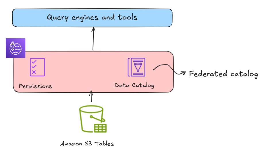
Validate the SageMaker Lakehouse table

You can now query your SageMaker Lakehouse table, created through zero-ETL integration, using various query engines. Complete the following steps to verify you can you see the table in SageMaker Unified Studio:

  1. Log in to the SageMaker Unified Studio portal using the single sign-on (SSO) option.

  1. Select your project to view its details page.

  1. Select Data in the navigation pane.

  1. Verify that you can see the Iceberg table in the SageMaker Lakehouse catalog.

Query with Athena

In this section, we show how to use Athena to query the SageMaker Lakehouse table from SageMaker Unified Studio. On the project page, locate the ecommerce_customer_behavior table in the catalog, and on the options menu (three dots), select Query with Athena.

This creates a SELECT query against the SageMaker Lakehouse table in a new window, and you should see the query results as shown in the following screenshot.

Query with Amazon Redshift

You can also query the SageMaker Lakehouse table from SageMaker Unified Studio using Amazon Redshift. Complete the following steps:

  1. Select the connection on the top right.
  2. Select Redshift (Lakehouse) from the list of connections.
  3. Select the awsdatacatalog database.
  4. Select the salesmarketing schema.
  5. Select Choose button.

The results will be shown in the Amazon Redshift Query Editor.

Query with Amazon EMR Serverless

You can query the Lakehouse table using Amazon EMR Serverless, which uses Apache Spark’s processing capabilities. Complete the following steps:

  1. On the project page, select Compute in the navigation pane.
  2. Select Add compute on the Data processing tab to create an EMR Serverless compute associated to the project.

  1. You can create new compute resources or connect to existing resources. For this example, select Create new compute resources.

  1. Select EMR Serverless.

  1. Enter a compute name (for example, Sales-Marketing), select the most recent release of EMR Serverless, and select Add compute.

It will take some time to create the compute.

You should see the status as Started for the compute. Now it’s ready to be used as your compute option for querying through a Jupyter notebook.

  1. Select the Build menu and select JupyterLab.

It will take some time to set up the workspace for running JupyterLab.

After the Jupyter Lab space is set up, you should see a page similar to the following screenshot.

  1. Select the new folder icon to create a new folder.

  1. Name the folder lakehouse_zetl_lab.

  1. Navigate to the folder you just created and create a notebook under this folder.
  1. Select the notebook Python3 (ipykernel) on the Launcher tab, and rename the notebook to query_lakehouse_table.

You can observe that the notebook is showing local Python as default language and compute. The two drop down menus show the connection type and compute for the selected connection type, just above the first cell within the Jupyter notebook.

  1. Select PySpark as the connection, and select the EMR Serverless application as compute.

  1. Enter the following sample code to query the table using Spark SQL:
import sys
from pyspark.sql import SparkSession
from pyspark.sql.functions import *

# Set the current database
spark.catalog.setCurrentDatabase("salesmarketing_XXX")

# Execute SQL query and store results in DataFrame
df = spark.sql("select * from ecommerce_customer_behavior limit 10")

# Display the results
df.show()

You can see the Spark DataFrame results.
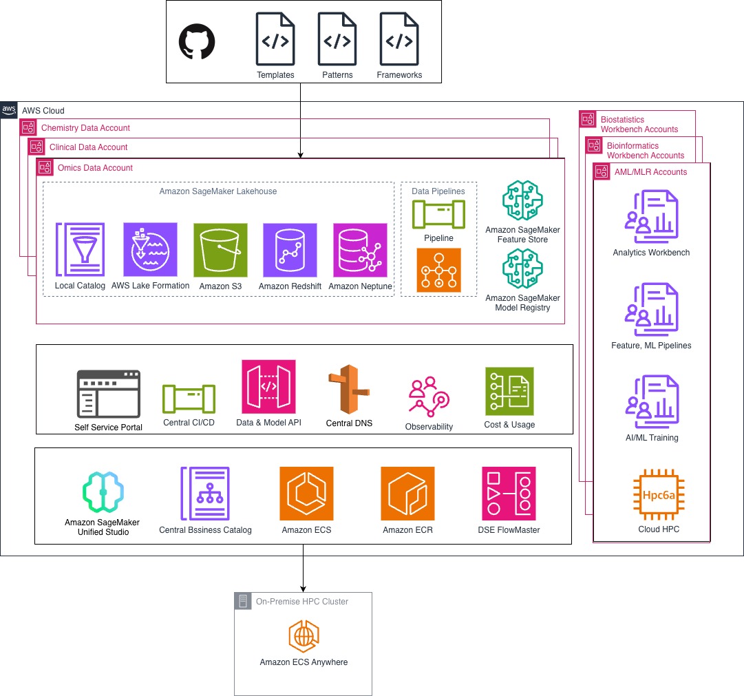
Clean up

To avoid incurring future charges, delete the SageMaker domain, DynamoDB table, AWS Glue resources, and other objects created from this post.

Conclusion

This post demonstrated how you can establish a zero-ETL connection from DynamoDB to SageMaker Lakehouse, making your data available in Iceberg format without building custom data pipelines. We showed how you can analyze this DynamoDB data through various compute engines within SageMaker Unified Studio. This streamlined approach alleviates traditional data movement complexities, and enables more efficient data analysis workflows directly from your DynamoDB tables.
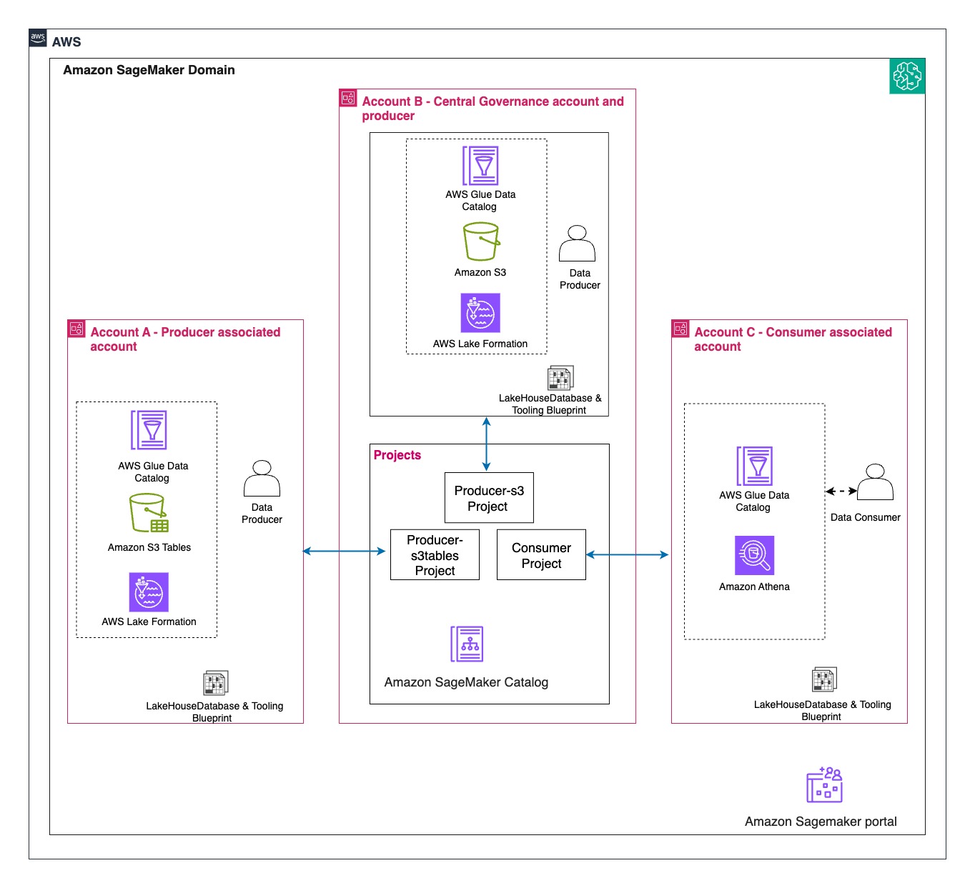
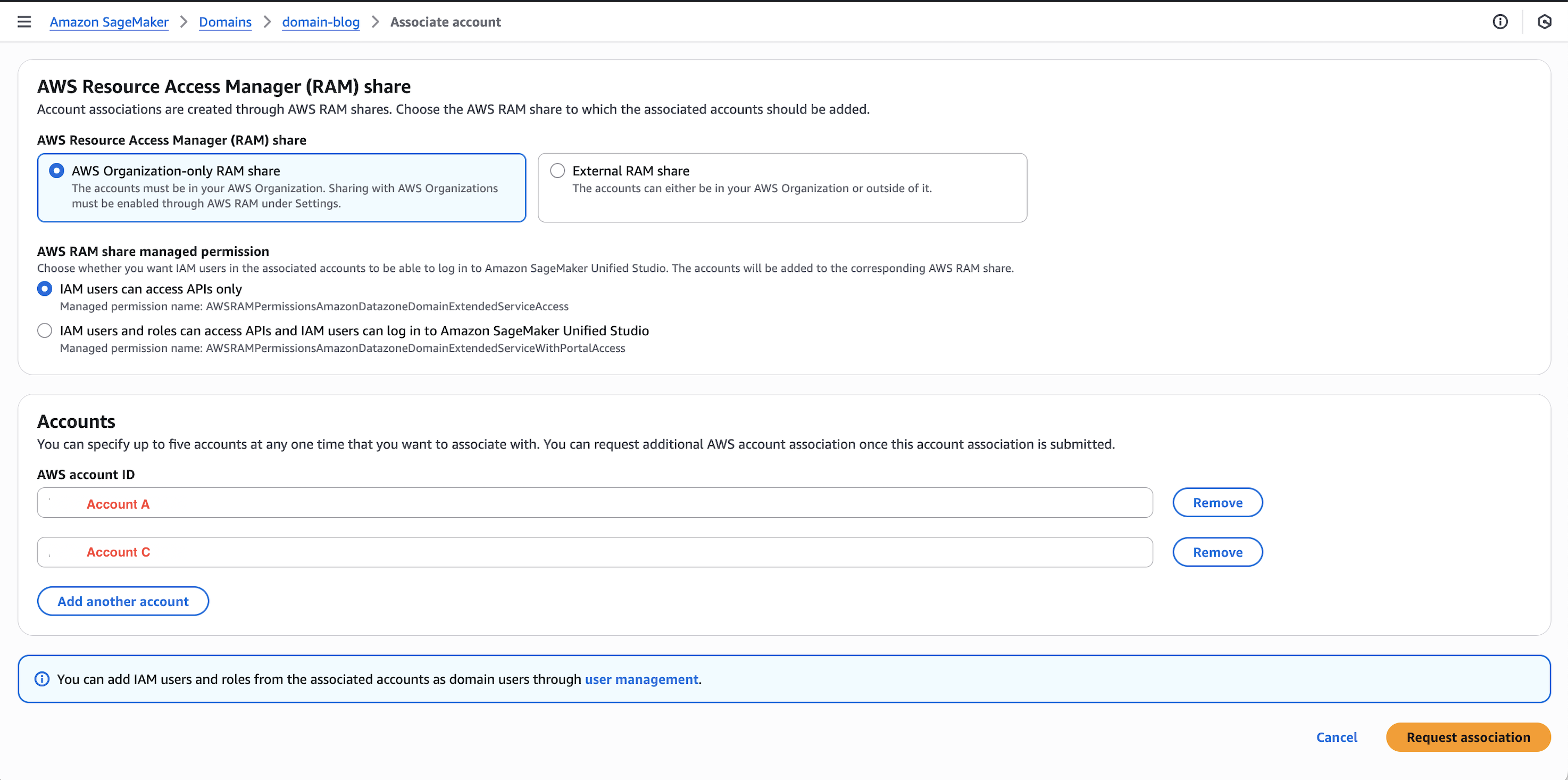
Try out this solution for your own use case, and share your feedback in the comments.
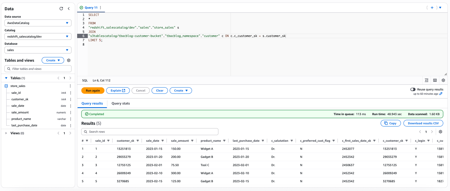

About the authors

Narayani Ambashta is an Analytics Specialist Solutions Architect at AWS, focusing on the automotive and manufacturing sector, where she guides strategic customers in developing modern data and AI strategies. With over 15 years of cross-industry experience, she specializes in big data architecture, real-time analytics, and AI/ML technologies, helping organizations implement modern data architectures. Her expertise spans across lakehouse, generative AI, and IoT platforms, enabling customers to drive digital transformation initiatives. When not architecting modern solutions, she enjoys staying active through sports and yoga.
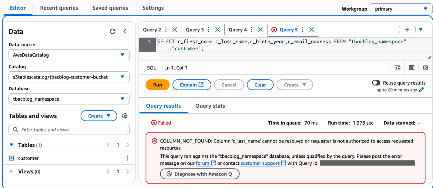
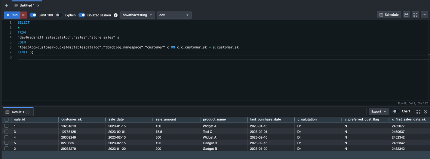
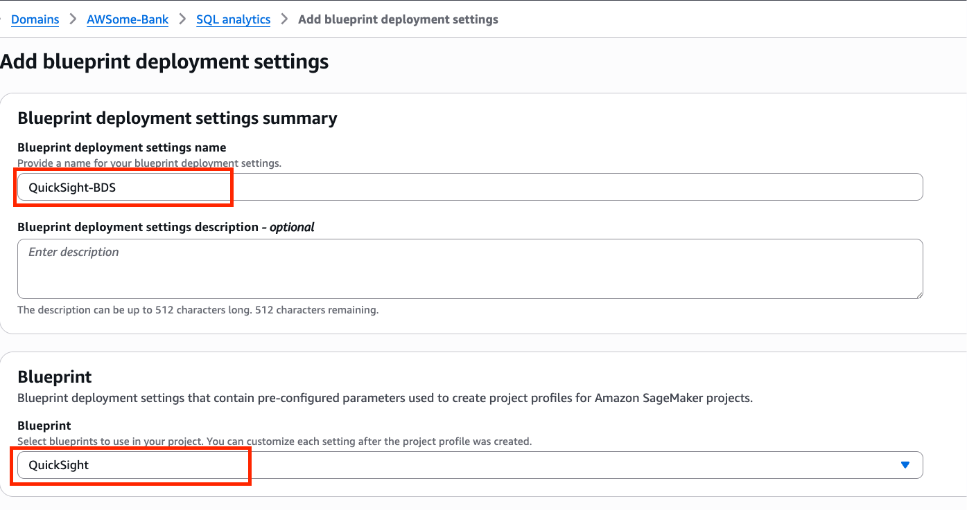
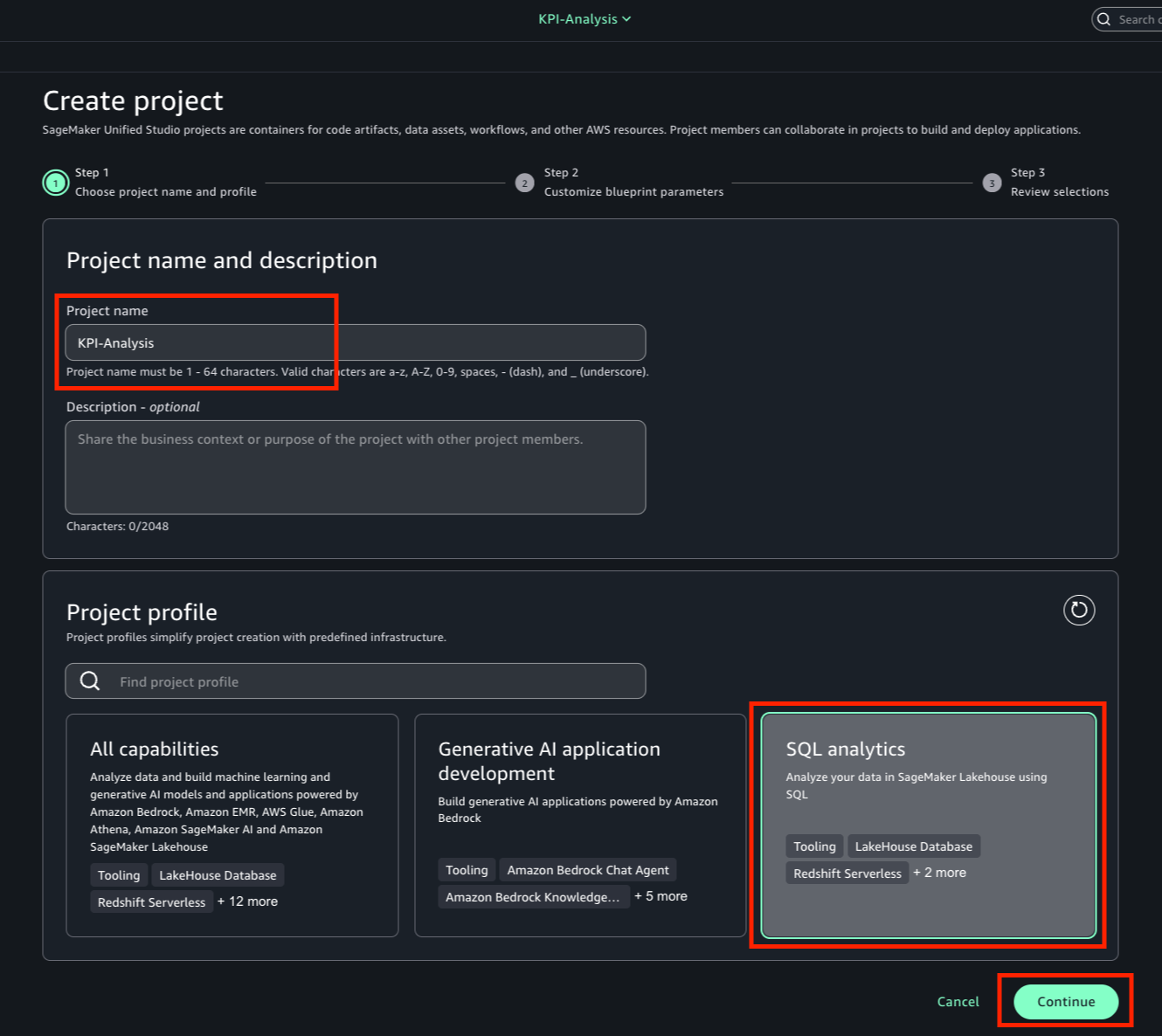
Raj Ramasubbu is a Senior Analytics Specialist Solutions Architect focused on big data and analytics and AI/ML with AWS. He helps customers architect and build highly scalable, performant, and secure cloud-based solutions on AWS. Raj provided technical expertise and leadership in building data engineering, big data analytics, business intelligence, and data science solutions for over 18 years prior to joining AWS. He helped customers in various industry verticals like healthcare, medical devices, life sciences, retail, asset management, car insurance, residential REIT, agriculture, title insurance, supply chain, document management, and real estate.

Yadgiri Pottabhathini is a Senior Analytics Specialist Solutions Architect in the media and entertainment sector. He specializes in assisting enterprise customers with their data and analytics cloud transformation initiatives, while providing guidance on accelerating their Generative AI adoption through the development of data foundations and modern data strategies that leverage open-source frameworks and technologies.

Junpei Ozono is a Sr. Go-to-market (GTM) Data & AI solutions architect at AWS in Japan. He drives technical market creation for data and AI solutions while collaborating with global teams to develop scalable GTM motions. He guides organizations in designing and implementing innovative data-driven architectures powered by AWS services, helping customers accelerate their cloud transformation journey through modern data and AI solutions. His expertise spans across modern data architectures including Data Mesh, Data Lakehouse, and Generative AI, enabling customers to build scalable and innovative solutions on AWS.

Unify streaming and analytical data with Amazon Data Firehose and Amazon SageMaker Lakehouse

Post Syndicated from Kalyan Janaki original https://aws.amazon.com/blogs/big-data/unify-streaming-and-analytical-data-with-amazon-data-firehose-and-amazon-sagemaker-lakehouse/

Organizations are increasingly required to derive real-time insights from their data while maintaining the ability to perform analytics. This dual requirement presents a significant challenge: how to effectively bridge the gap between streaming data and analytical workloads without creating complex, hard-to-maintain data pipelines. In this post, we demonstrate how to simplify this process using Amazon Data Firehose (Firehose) to deliver streaming data directly to Apache Iceberg tables in Amazon SageMaker Lakehouse, creating a streamlined pipeline that reduces complexity and maintenance overhead.

Streaming data empowers AI and machine learning (ML) models to learn and adapt in real time, which is crucial for applications that require immediate insights or dynamic responses to changing conditions. This creates new opportunities for business agility and innovation. Key use cases include predicting equipment failures based on sensor data, monitoring supply chain processes in real time, and enabling AI applications to respond dynamically to changing conditions. Real-time streaming data helps customers make quick decisions, fundamentally changing how businesses compete in real-time markets.

Amazon Data Firehose seamlessly acquires, transforms, and delivers data streams to lakehouses, data lakes, data warehouses, and analytics services, with automatic scaling and delivery within seconds. For analytical workloads, a lakehouse architecture has emerged as an effective solution, combining the best elements of data lakes and data warehouses. Apache Iceberg, an open table format, enables this transformation by providing transactional guarantees, schema evolution, and efficient metadata handling that were previously only available in traditional data warehouses. SageMaker Lakehouse unifies your data across Amazon Simple Storage Service (Amazon S3) data lakes, Amazon Redshift data warehouses, and other sources, and gives you the flexibility to access your data in-place with Iceberg-compatible tools and engines. By using SageMaker Lakehouse, organizations can harness the power of Iceberg while benefiting from the scalability and flexibility of a cloud-based solution. This integration removes the traditional barriers between data storage and ML processes, so data workers can work directly with Iceberg tables in their preferred tools and notebooks.

In this post, we show you how to create Iceberg tables in Amazon SageMaker Unified Studio and stream data to these tables using Firehose. With this integration, data engineers, analysts, and data scientists can seamlessly collaborate and build end-to-end analytics and ML workflows using SageMaker Unified Studio, removing traditional silos and accelerating the journey from data ingestion to production ML models.

Solution overview

The following diagram illustrates the architecture of how Firehose can deliver real-time data to SageMaker Lakehouse.

This post includes an AWS CloudFormation template to set up supporting resources so Firehose can deliver streaming data to Iceberg tables. You can review and customize it to suit your needs. The template performs the following operations:

Prerequisites

For this walkthrough, you should have the following prerequisites:

After you create the prerequisites, verify you can log in to SageMaker Unified Studio and the project is created successfully. Every project created in SageMaker Unified Studio gets a project location and project IAM role, as highlighted in the following screenshot.

Create an Iceberg table

For this solution, we use Amazon Athena as the engine for our query editor. Complete the following steps to create your Iceberg table:

  1. In SageMaker Unified Studio, on the Build menu, choose Query Editor.

  1. Choose Athena as the engine for query editor and choose the AWS Glue database created for the project.

  1. Use the following SQL statement to create the Iceberg table. Make sure to provide your project AWS Glue database and project Amazon S3 location (can be found on the project overview page):
CREATE TABLE firehose_events (
type struct<device: string, event: string, action: string>,
customer_id string,
event_timestamp timestamp,
region string)
LOCATION '<PROJECT_S3_LOCATION>/iceberg/events'
TBLPROPERTIES (
'table_type'='iceberg',
'write_compression'='zstd'
);

Deploy the supporting resources

The next step is to deploy the required resources into your AWS environment by using a CloudFormation template. Complete the following steps:

  1. Choose Launch Stack.
  2. Choose Next.
  3. Leave the stack name as firehose-lakehouse.
  4. Provide the user name and password that you want to use for accessing the Amazon Kinesis Data Generator application.
  5. For DatabaseName, enter the AWS Glue database name.
  6. For ProjectBucketName, enter the project bucket name (located on the SageMaker Unified Studio project details page).
  7. For TableName, enter the table name created in SageMaker Unified Studio.
  8. Choose Next.

  1. Select I acknowledge that AWS CloudFormation might create IAM resources and choose Next.

  1. Complete the stack.

Create a Firehose stream

Complete the following steps to create a Firehose stream to deliver data to Amazon S3:

  1. On the Firehose console, choose Create Firehose stream.

  1. For Source, choose Direct PUT.
  2. For Destination, choose Apache Iceberg Tables.

This example chooses Direct PUT as the source, but you can apply the same steps for other Firehose sources, such as Amazon Kinesis Data Streams and Amazon Managed Streaming for Apache Kafka (Amazon MSK).

  1. For Firehose stream name, enter firehose-iceberg-events.

  1. Collect the database name and table name from the SageMaker Unified Studio project to use in the next step.

  1. In the Destination settings section, enable Inline parsing for routing information and provide the database name and table name from the previous step.

Make sure you enclose the database and table names in double quotes if you want to deliver data to a single database and table. Amazon Data Firehose can also route records to different tables based on the content of the record. For more information, refer to Route incoming records to different Iceberg tables.

  1. Under Buffer hints, reduce the buffer size to 1 MiB and the buffer interval to 60 seconds. You can fine-tune these settings based on your use case latency needs.

  1. In the Backup settings section, enter the S3 bucket created by the CloudFormation template (s3://firehose-demo-iceberg-<account_id>-<region>) and the error output prefix (error/events-1/).

  1. In the Advanced settings section, enable Amazon CloudWatch error logging to troubleshoot any failures, and in for Existing IAM roles, choose the role that starts with Firehose-Iceberg-Stack-FirehoseIamRole-*, created by the CloudFormation template.
  2. Choose Create Firehose stream.

Generate streaming data

Use the Amazon Kinesis Data Generator to publish data records into your Firehose stream:

  1. On the AWS CloudFormation console, choose Stacks in the navigation pane and open your stack.
  2. Select the nested stack for the generator, and go to the Outputs tab.
  3. Choose the Amazon Kinesis Data Generator URL.

  1. Enter the credentials that you defined when deploying the CloudFormation stack.

  1. Choose the AWS Region where you deployed the CloudFormation stack and choose your Firehose stream.
  2. For the template, replace the default values with the following code:
{
"type": {
"device": "{{random.arrayElement(["mobile", "desktop", "tablet"])}}",
"event": "{{random.arrayElement(["firehose_events_1", "firehose_events_2"])}}",
"action": "update"
},
"customer_id": "{{random.number({ "min": 1, "max": 1500})}}",
"event_timestamp": "{{date.now("YYYY-MM-DDTHH:mm:ss.SSS")}}",
"region": "{{random.arrayElement(["pdx", "nyc"])}}"
}
  1. Before sending data, choose Test template to see an example payload.
  2. Choose Send data.

You can monitor the progress of the data stream.

Query the table in SageMaker Unified Studio

Now that Firehose is delivering data to SageMaker Lakehouse, you can perform analytics on that data in SageMaker Unified Studio using different AWS analytics services.

Clean up

It’s generally a good practice to clean up the resources created as part of this post to avoid additional cost. Complete the following steps:

  1. On the AWS CloudFormation console, choose Stacks in the navigation pane.
  2. Select the stack firehose-lakehouse* and on the Actions menu, choose Delete Stack.
  3. In SageMaker Unified Studio, delete the domain created for this post.

Conclusion

Streaming data allows models to make predictions or decisions based on the latest information, which is crucial for time-sensitive applications. By incorporating real-time data, models can make more accurate predictions and decisions. Streaming data can help organizations avoid the costs associated with storing and processing large datasets, because it focuses on the most relevant information. Amazon Data Firehose makes it straightforward to bring real-time streaming data to data lakes in Iceberg format and unifying it with other data assets in SageMaker Lakehouse, making streaming data accessible by various analytics and AI services in SageMaker Unified Studio to deliver real-time insights. Try out the solution for your own use case, and share your feedback and questions in the comments.


About the Authors

Kalyan Janaki is Senior Big Data & Analytics Specialist with Amazon Web Services. He helps customers architect and build highly scalable, performant, and secure cloud-based solutions on AWS.

Phaneendra Vuliyaragoli is a Product Management Lead for Amazon Data Firehose at AWS. In this role, Phaneendra leads the product and go-to-market strategy for Amazon Data Firehose.

Maria Ho is a Product Marketing Manager for Streaming and Messaging services at AWS. She works with services including Amazon Managed Streaming for Apache Kafka (Amazon MSK), Amazon Managed Service for Apache Flink, Amazon Data Firehose, Amazon Kinesis Data Streams, Amazon MQ, Amazon Simple Queue Service (Amazon SQS), and Amazon Simple Notification Services (Amazon SNS).