[$] Linux ecosystem contributions from SteamOS

Post Syndicated from jake original https://lwn.net/Articles/946188/

The SteamOS Linux
distribution is focused on gaming, naturally, but the effort to build it
has resulted
in contributions to multiple areas in the Linux ecosystem. Alberto Garcia
has been working on SteamOS and came to Bilbao, Spain to describe some of those
contributions at Open Source Summit Europe 2023. There are some obvious
areas where a gaming-focused OS might contribute upstream, such as
graphics, but the talk showed contributions in several other areas as well.

A local root vulnerability in glibc

Post Syndicated from corbet original https://lwn.net/Articles/946381/

Qualys has posted an
advisory
for a vulnerability in the GNU C Library related to the
handling of the GLIBC_TUNABLES environment variable:

We successfully exploited this vulnerability and obtained full root
privileges on the default installations of Fedora 37 and 38, Ubuntu
22.04 and 23.04, Debian 12 and 13; other distributions are probably
also vulnerable and exploitable (one notable exception is Alpine
Linux, which uses musl libc, not the glibc).

Updates from distributors are beginning to appear and should be applied on
any systems with untrusted users.
The curious can see the fix applied to glibc in this
patch series
.

Falcon Northwest RAK Intel Xeon W-3400 Unleashed Edition

Post Syndicated from Patrick Kennedy original https://www.servethehome.com/falcon-northwest-rak-intel-xeon-w-3400-unleashed-edition-nvidia-asus-silverstone-kingston/

In our Falcon Northwest RAK review, we see how the company unleashed the Intel Xeon w9-3495X as a fast workstation today and a server tomorrow

The post Falcon Northwest RAK Intel Xeon W-3400 Unleashed Edition appeared first on ServeTheHome.

Migrate an existing data lake to a transactional data lake using Apache Iceberg

Post Syndicated from Rajdip Chaudhuri original https://aws.amazon.com/blogs/big-data/migrate-an-existing-data-lake-to-a-transactional-data-lake-using-apache-iceberg/

A data lake is a centralized repository that you can use to store all your structured and unstructured data at any scale. You can store your data as-is, without having to first structure the data and then run different types of analytics for better business insights. Over the years, data lakes on Amazon Simple Storage Service (Amazon S3) have become the default repository for enterprise data and are a common choice for a large set of users who query data for a variety of analytics and machine leaning use cases. Amazon S3 allows you to access diverse data sets, build business intelligence dashboards, and accelerate the consumption of data by adopting a modern data architecture or data mesh pattern on Amazon Web Services (AWS).

Analytics use cases on data lakes are always evolving. Oftentimes, you want to continuously ingest data from various sources into a data lake and query the data concurrently through multiple analytics tools with transactional capabilities. But traditionally, data lakes built on Amazon S3 are immutable and don’t provide the transactional capabilities needed to support changing use cases. With changing use cases, customers are looking for ways to not only move new or incremental data to data lakes as transactions, but also to convert existing data based on Apache Parquet to a transactional format. Open table formats, such as Apache Iceberg, provide a solution to this issue. Apache Iceberg enables transactions on data lakes and can simplify data storage, management, ingestion, and processing.

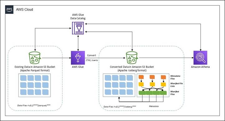
In this post, we show you how you can convert existing data in an Amazon S3 data lake in Apache Parquet format to Apache Iceberg format to support transactions on the data using Jupyter Notebook based interactive sessions over AWS Glue 4.0.

Existing Parquet to Iceberg migration

There are two broad methods to migrate the existing data in a data lake in Apache Parquet format to Apache Iceberg format to convert the data lake to a transactional table format.

In-place data upgrade

In an in-place data migration strategy, existing datasets are upgraded to Apache Iceberg format without first reprocessing or restating existing data. This means the data files in the data lake aren’t modified during the migration and all Apache Iceberg metadata files (manifests, manifest files, and table metadata files) are generated outside the purview of the data. In this method, the metadata are recreated in an isolated environment and colocated with the existing data files. This can be a much less expensive operation compared to rewriting all the data files. The existing data file format must be Apache Parquet, Apache ORC, or Apache Avro. An in-place migration can be performed in either of two ways:

  1. Using add_files: This procedure adds existing data files to an existing Iceberg table with a new snapshot that includes the files. Unlike migrate or snapshot, add_files can import files from a specific partition or partitions and doesn’t create a new Iceberg table. This procedure doesn’t analyze the schema of the files to determine if they match the schema of the Iceberg table. Upon completion, the Iceberg table treats these files as if they are part of the set of files owned by Apache Iceberg.
  2. Using migrate: This procedure replaces a table with an Apache Iceberg table loaded with the source’s data files. The table’s schema, partitioning, properties, and location are copied from the source table. Supported formats are Avro, Parquet, and ORC. By default, the original table is retained with the name table_BACKUP_. However, to leave the original table intact during the process, you must use snapshot to create a new temporary table that has the same source data files and schema.

In this post, we show you how you can use the Iceberg add_files procedure for an in-place data upgrade. Note that the migrate procedure isn’t supported in AWS Glue Data Catalog.

The following diagram shows a high-level representation.

CTAS migration of data

The create table as select (CTAS) migration approach is a technique where all the metadata information for Iceberg is generated along with restating all the data files. This method shadows the source dataset in batches. When the shadow is caught up, you can swap the shadowed dataset with the source.

The following diagram showcases the high-level flow.

Prerequisites

To follow along with the walkthrough, you must have the following:

You can check the data size using the following code in the AWS CLI or AWS CloudShell:

//Run this command to check the data size

aws s3 ls --summarize --human-readable --recursive s3://noaa-ghcn-pds/parquet/by_year/YEAR=2023

As of writing this post, there are 107 objects with total size of 70 MB for year 2023 in the Amazon S3 path.

Note that to implement the solution, you must complete a few preparatory steps.

Deploy resources using AWS CloudFormation

Complete the following steps to create the S3 bucket and the AWS IAM role and policy for the solution:

  1. Sign in to your AWS account and then choose Launch Stack to launch the CloudFormation template.

  1. For Stack name, enter a name.
  2. Leave the parameters at the default values. Note that if the default values are changed, then you must make corresponding changes throughout the following steps.
  3. Choose Next to create your stack.

This AWS CloudFormation template deploys the following resources:

  • An S3 bucket named demo-blog-post-XXXXXXXX (XXXXXXXX represents the AWS account ID used).
  • Two folders named parquet and iceberg under the bucket.
  • An IAM role and a policy named demoblogpostrole and demoblogpostscoped respectively.
  • An AWS Glue database named ghcn_db.
  • An AWS Glue Crawler named demopostcrawlerparquet.

After the the AWS CloudFormation template is successfully deployed:

  1. Copy the data in the created S3 bucket using following command in AWS CLI or AWS CloudShell. Replace XXXXXXXX appropriately in the target S3 bucket name.
    Note: In the example, we copy data only for the year 2023. However, you can work with the entire dataset, following the same instructions.

    aws s3 sync s3://noaa-ghcn-pds/parquet/by_year/YEAR=2023/ s3://demo-blog-post-XXXXXXXX/parquet/year=2023

  2. Open the AWS Management Console and go to the AWS Glue console.
  3. On the navigation pane, select Crawlers.
  4. Run the crawler named demopostcrawlerparquet.
  5. After the AWS Glue crawler demopostcrawlerparquet is successfully run, the metadata information of the Apache Parquet data will be cataloged under the ghcn_db AWS Glue database with the table name source_parquet. Notice that the table is partitioned over year and element columns (as in the S3 bucket).

  1. Use the following query to verify the data from the Amazon Athena console. If you’re using Amazon Athena for the first time in your AWS Account, set up a query result location in Amazon S3.
    SELECT * FROM ghcn_db.source_parquet limit 10;

Launch an AWS Glue Studio notebook for processing

For this post, we use an AWS Glue Studio notebook. Follow the steps in Getting started with notebooks in AWS Glue Studio to set up the notebook environment. Launch the notebooks hosted under this link and unzip them on a local workstation.

  1. Open AWS Glue Studio.
  2. Choose ETL Jobs.
  3. Choose Jupyter notebook and then choose Upload and edit an existing notebook. From Choose file, select required ipynb file and choose Open, then choose Create.
  4. On the Notebook setup page, for Job name, enter a logical name.
  5. For IAM role, select demoblogpostrole. Choose Create job. After a minute, the Jupyter notebook editor appears. Clear all the default cells.

The preceding steps launch an AWS Glue Studio notebook environment. Make sure you Save the notebook every time it’s used.

In-place data upgrade

In this section we show you how you can use the add_files procedure to achieve an in-place data upgrade. This section uses the ipynb file named demo-in-place-upgrade-addfiles.ipynb. To use with the add_files procedure, complete the following:

  1. On the Notebook setup page, for Job name, enter demo-in-place-upgrade for the notebook session as explained in Launch Glue notebook for processing.
  2. Run the cells under the section Glue session configurations. Provide the S3 bucket name from the prerequisites for the bucket_name variable by replacing XXXXXXXX.
  3. Run the subsequent cells in the notebook.

Notice that the cell under Execute add_files procedure section performs the metadata creation in the mentioned path.

Review the data file paths for the new Iceberg table. To show an Iceberg table’s current data files, .files can be used to get details such as file_path, partition, and others. Recreated files are pointing to the source path under Amazon S3.

Note the metadata file location after transformation. It’s pointing to the new folder named iceberg under Amazon S3. This can be checked using .snapshots to check Iceberg tables’ snapshot file location. Also, check the same in the Amazon S3 URI s3://demo-blog-post-XXXXXXXX/iceberg/ghcn_db.db/target_iceberg_add_files/metadata/. Also notice that there are two versions of the manifest list created after the add_files procedure has been run. The first is an empty table with the data schema and the second is adding the files.

The table is cataloged in AWS Glue under the database ghcn_db with the table type as ICEBERG.

Compare the count of records using Amazon Athena between the source and target table. They are the same.

In summary, you can use the add_files procedure to convert existing data files in Apache Parquet format in a data lake to Apache Iceberg format by adding the metadata files and without recreating the table from scratch. Following are some pros and cons of this method.

Pros

  • Avoids full table scans to read the data as there is no restatement. This can save time.
  • If there are any errors during while writing the metadata, only a metadata re-write is required and not the entire data.
  • Lineage of the existing jobs is maintained because the existing catalog still exists.

Cons

  • If data is processed (inserts, updates, and deletes) in the dataset during the metadata writing process, the process must be run again to include the new data.
  • There must be write downtime to avoid having to run the process a second time.
  • If a data restatement is required, this workflow will not work as source data files aren’t modified.

CTAS migration of data

This section uses the ipynb file named demo-ctas-upgrade.ipynb. Complete the following:

  1. On the Notebook setup page, for Job name, enter demo-ctas-upgrade for the notebook session as explained under Launch Glue notebook for processing.
  2. Run the cells under the section Glue session configurations. Provide the S3 bucket name from the prerequisites for the bucket_name variable by replacing XXXXXXXX.
  3. Run the subsequent cells in the notebook.

Notice that the cell under Create Iceberg table from Parquet section performs the shadow upgrade to Iceberg format. Note that Iceberg requires sorting the data according to table partitions before writing to the Iceberg table. Further details can be found in Writing Distribution Modes.

Notice the data and metadata file paths for the new Iceberg table. It’s pointing to the new path under Amazon S3. Also, check under the Amazon S3 URI s3://demo-blog-post-XXXXXXXX/iceberg/ghcn_db.db/target_iceberg_ctas/ used for this post.

The table is cataloged under AWS Glue under the database ghcn_db with the table type as ICEBERG.

Compare the count of records using Amazon Athena between the source and target table. They are same.

In summary, the CTAS method creates a new table by generating all the metadata files along with restating the actual data. Following are some pros and cons of this method:

Pros

  • It allows you to audit and validate the data during the process because data is restated.
  • If there are any runtime issues during the migration process, rollback and recovery can be easily performed by deleting the Apache Iceberg table.
  • You can test different configurations when migrating a source. You can create a new table for each configuration and evaluate the impact.
  • Shadow data is renamed to a different directory in the source (so it doesn’t collide with old Apache Parquet data).

Cons

  • Storage of the dataset is doubled during the process as both the original Apache Parquet and new Apache Iceberg tables are present during the migration and testing phase. This needs to be considered during cost estimation.
  • The migration can take much longer (depending on the volume of the data) because both data and metadata are written.
  • It’s difficult to keep tables in sync if there changes to the source table during the process.

Clean up

To avoid incurring future charges, and to clean up unused roles and policies, delete the resources you created: the datasets, CloudFormation stack, S3 bucket, AWS Glue job, AWS Glue database, and AWS Glue table.

Conclusion

In this post, you learned strategies for migrating existing Apache Parquet formatted data to Apache Iceberg in Amazon S3 to convert to a transactional data lake using interactive sessions in AWS Glue 4.0 to complete the processes. If you have an evolving use case where an existing data lake needs to be converted to a transactional data lake based on Apache Iceberg table format, follow the guidance in this post.

The path you choose for this upgrade, an in-place upgrade or CTAS migration, or a combination of both, will depend on careful analysis of the data architecture and data integration pipeline. Both pathways have pros and cons, as discussed. At a high level, this upgrade process should go through multiple well-defined phases to identify the patterns of data integration and use cases. Choosing the correct strategy will depend on your requirements—such as performance, cost, data freshness, acceptable downtime during migration, and so on.


About the author

Rajdip Chaudhuri is a Senior Solutions Architect with Amazon Web Services specializing in data and analytics. He enjoys working with AWS customers and partners on data and analytics requirements. In his spare time, he enjoys soccer and movies.

Apache Iceberg optimization: Solving the small files problem in Amazon EMR

Post Syndicated from Avijit Goswami original https://aws.amazon.com/blogs/big-data/apache-iceberg-optimization-solving-the-small-files-problem-in-amazon-emr/

In our previous post Improve operational efficiencies of Apache Iceberg tables built on Amazon S3 data lakes, we discussed how you can implement solutions to improve operational efficiencies of your Amazon Simple Storage Service (Amazon S3) data lake that is using the Apache Iceberg open table format and running on the Amazon EMR big data platform. Iceberg tables store metadata in manifest files. As the number of data files increase, the amount of metadata stored in these manifest files also increases, leading to longer query planning time. The query runtime also increases because it’s proportional to the number of data or metadata file read operations. Compaction is the process of combining these small data and metadata files to improve performance and reduce cost. Compaction also gets rid of deleting files by applying deletes and rewriting a new file without deleting records. Currently, Iceberg provides a compaction utility that compacts small files at a table or partition level. But this approach requires you to implement the compaction job using your preferred job scheduler or manually triggering the compaction job.

In this post, we discuss the new Iceberg feature that you can use to automatically compact small files while writing data into Iceberg tables using Spark on Amazon EMR or Amazon Athena.

Use cases for processing small files

Streaming applications are prone to creating a large number of small files, which can negatively impact the performance of subsequent processing times. For example, consider a critical Internet of Things (IoT) sensor from a cold storage facility that is continuously sending temperature and health data into an S3 data lake for downstream data processing and triggering actions like emergency maintenance. Systems of this nature generate a huge number of small objects and need attention to compact them to a more optimal size for faster reading, such as 128 MB, 256 MB, or 512 MB. In this post, we show you a streaming sensor data use case with a large number of small files and the mitigation steps using the Iceberg open table format. For more information on streaming applications on AWS, refer to Real-time Data Streaming and Analytics.

Streaming Architecture

Solution overview

To compact the small files for improved performance, in this example, Amazon EMR triggers a compaction job after the write commit as a post-commit hook when defined thresholds (for example, number of commits) are met. By default, Amazon EMR waits for 10 commits to trigger the post-commit hook compaction utility.

This Iceberg event-based table management feature lets you monitor table activities during writes to make better decisions about how to manage each table differently based on events. As of this writing, only the optimize-data optimization is supported. To learn more about the available optimize data executors and catalog properties, refer to the README file in the GitHub repo.

To use the feature, you can use the iceberg-aws-event-based-table-management source code and provide the built JAR in the engine’s class-path. The following bootstrap action can place the JAR in the engine’s class-path:

sudo aws s3 cp s3://<path>/iceberg-aws-event-based-table-management-0.1.jar /usr/lib/spark/jars/

Note that the Iceberg AWS event-based table management feature works with Iceberg v1.2.0 and above (available from Amazon EMR 6.11.0).

In some use cases, you may want to run the event-based compaction jobs in a different EMR cluster in order to avoid any impact to the ETL jobs running in their current EMR cluster. You can get the metadata, including the cluster ID of your current ETL workflows, from the /mnt/var/lib/info/job-flow.json file and then use a different cluster to process the event-based compactions.

The notebook examples shown in the following sections are also available in the aws-samples GitHub repo.

Prerequisite

For this performance comparison exercise between a Spark external table and an Iceberg table and Iceberg with compaction, we generate a significant number of small files in Parquet format and store them in an S3 bucket. We used the Amazon Kinesis Data Generator (KDG) tool to generate sample sensor data information using the following template:

{"sensorId": {{random.number(5000)}},
 "currentTemperature": {{random.number(
        {
            "min":10,
            "max":150
        }
  )}},
 "status": "{{random.arrayElement(
        ["OK","FAIL","WARN"]
    )}}",
 "date_ts": "{{date.now("YYYY-MM-DD HH:mm:ss")}}"
}

We configured an Amazon Kinesis Data Firehose delivery stream and sent the generated data into a staging S3 bucket. Then we ran an AWS Glue extract, transform, and load (ETL) job to convert the JSON files into Parquet format. For our testing, we generated about 58,176 small objects with total size of 2 GB.

For running the Amazon EMR tests, we used Amazon EMR version emr-6.11.0 with Spark 3.3.2, and JupyterEnterpriseGateway 2.6.0. The cluster used had one primary node (r5.2xlarge) and two core nodes (r5.xlarge). We used a bootstrap action during cluster creation to enable event-based table management:

sudo aws s3 cp s3://<path>/iceberg-aws-event-based-table-management-0.1.jar /usr/lib/spark/jars/

Also, refer to our guidance on how to use an Iceberg cluster with Spark, which is a prerequisite for this exercise.

As part of the exercise, we see new steps are being added to the EMR cluster to trigger the compaction jobs. To enable adding new steps to the running cluster, we add the elasticmapreduce:AddJobFlowSteps action to the cluster’s default role, EMR_EC2_DefaultRole, as a prerequisite.

Performance of Iceberg reads with the compaction utility on Amazon EMR

In the following steps, we demonstrate how to use the compaction utility and what performance benefits you can achieve. We use an EMR notebook to demonstrate the benefits of the compaction utility. For instructions to set up an EMR notebook, refer to Amazon EMR Studio overview.

First, you configure your Spark session using the %%configure magic command. We use the Hive catalog for Iceberg tables.

  1. Before you run the following step, create an Amazon S3 bucket in your AWS account called <your-iceberg-storage-blog>. To check how to create an Amazon S3 bucket, follow the instructions given here. Update the your-iceberg-storage-blog bucket name in the following configuration with the actual bucket name you created to test this example:
    %%configure -f
    {
    "conf":{
        "spark.sql.extensions":"org.apache.iceberg.spark.extensions.IcebergSparkSessionExtensions",
        "spark.sql.catalog.dev":"org.apache.iceberg.spark.SparkCatalog",
        "spark.sql.catalog.dev.catalog-impl":"org.apache.iceberg.aws.glue.GlueCatalog",
        "spark.sql.catalog.dev.io-impl":"org.apache.iceberg.aws.s3.S3FileIO",
        "spark.sql.catalog.dev.warehouse":"s3://<your-iceberg-storage-blog>/iceberg/"
        }
    }

  2. Create a new database for the Iceberg table in the AWS Glue Data Catalog named DB and provide the S3 URI specified in the Spark config as s3://<your-iceberg-storage-blog>/iceberg/db. Also, create another Database named iceberg_db in Glue for the parquet tables. Follow the instructions given in Working with databases on the AWS Glue console to create your Glue databases. Then create a new Spark table in Parquet format pointing to the bucket containing small objects in your AWS account. See the following code:
    spark.sql(""" CREATE TABLE iceberg_db.sensor_data_parquet_table (
        sensorid int,
        currenttemperature int,
        status string,
        date_ts timestamp)
    USING parquet
    location 's3://<your-bucket-with-parquet-files>/'
    """)

  3. Run an aggregate SQL to measure the performance of Spark SQL on the Parquet table with 58,176 small objects:
    spark.sql(""" select maxtemp, mintemp, avgtemp from
    (select
    max(currenttemperature) as maxtemp,
    min(currenttemperature) as mintemp,
    avg(currenttemperature) as avgtemp
    from iceberg_db.sensor_data_parquet_table
    where month(date_ts) between 2 and 10
    order by maxtemp, mintemp, avgtemp)""").show()

In the following steps, we create a new Iceberg table from the Spark/Parquet table using CTAS (Create Table As Select). Then we show how the automated compaction job can help improve query performance.

  1. Create a new Iceberg table using CTAS from the earlier AWS Glue table with the small files:
    spark.sql(""" CREATE TABLE dev.db.sensor_data_iceberg_format USING iceberg AS (SELECT * FROM iceberg_db.sensor_data_parquet_table)""")

  2. Validate that a new Iceberg snapshot was created for the new table:
    spark.sql(""" Select * from dev.db.sensor_data_iceberg_format.snapshots limit 5""").show()

We have confirmed that our S3 folder corresponds to the newly created Iceberg table. It shows that during the CTAS statement, it added 1,879 objects in the new folder with a total size of 1.3 GB. We can conclude that Iceberg did some optimization while loading data from the Parquet table.

  1. Now that you have data in the Iceberg table, run the previous aggregation SQL to check the runtime:
    spark.sql(""" select maxtemp, mintemp, avgtemp from
    (select
    max(currenttemperature) as maxtemp,
    min(currenttemperature) as mintemp,
    avg(currenttemperature) as avgtemp
    from dev.db.sensor_data_iceberg_format
    where month(date_ts) between 2 and 10
    order by maxtemp, mintemp, avgtemp)""").show()

The runtime for the preceding query ran on the Iceberg table with 1,879 objects in 1 minute, 39 seconds. There is already some significant performance improvement by converting the external Parquet table to an Iceberg table.

  1. Now let’s add the configurations needed to apply the automatic compaction of small files in the Iceberg tables. Note the last four newly added configurations in the following statement. The parameter optimize-data.commit-threshold suggests that the compaction will take place after the first successful commit. The default is 10 successful commits to trigger the compaction.
    %%configure -f
    {
    "conf":{
        "spark.sql.extensions":"org.apache.iceberg.spark.extensions.IcebergSparkSessionExtensions",
        "spark.sql.catalog.dev":"org.apache.iceberg.spark.SparkCatalog",
        "spark.sql.catalog.dev.catalog-impl":"org.apache.iceberg.aws.glue.GlueCatalog",
        "spark.sql.catalog.dev.io-impl":"org.apache.iceberg.aws.s3.S3FileIO",
        "spark.sql.catalog.dev.warehouse":"s3://<your-iceberg-storage-blog>/iceberg/",
        "spark.sql.catalog.dev.metrics-reporter-impl":"org.apache.iceberg.aws.manage.AwsTableManagementMetricsEvaluator",
        "spark.sql.catalog.dev.optimize-data.impl":"org.apache.iceberg.aws.manage.EmrOnEc2OptimizeDataExecutor",
        "spark.sql.catalog.dev.optimize-data.emr.cluster-id":"j-1N8J5NZI0KEU3",
        "spark.sql.catalog.dev.optimize-data.commit-threshold":"1"
        }
    }

  2. Run a quick sanity check to confirm that the configurations are working fine with Spark SQL.

  1. 10. To activate the automatic compaction process, add a new record to the existing Iceberg table using a Spark insert:
    spark.sql(""" Insert into dev.db.sensor_data_iceberg_format values(999123, 86, 'PASS', timestamp'2023-07-26 12:50:25') """)

  2. Navigate to the Amazon EMR console to check the cluster steps.

You should see a new step added that goes from Pending to Running and finally the Completed state. Every time the data in the Iceberg table is updated or inserted, based on configuration optimize-data.commit-threshold, the optimize job will automatically trigger to compact the underlying data.

  1. Validate that the record insert was successful.

  1. Check the snapshot table to see that a new snapshot is created for the table with the operation replace.

For every successful run of the background optimize job, a new entry will be added to the snapshot table.

  1. On the Amazon S3 console, navigate to the folder corresponding to the Iceberg table and see that the data files are compacted.

In our case, it was compacted from the previous smaller sizes to approximately 437 MB. The folder will still contain the previous smaller files for time travel unless you issue an expire snapshot command to remove them.

  1. Now you can run the same aggregate query and record the performance after the compaction.

Summary of Amazon EMR testing

The runtime for the preceding aggregation query on the compacted Iceberg table reduced to approximately 59 seconds from the previous runtime of 1 minute, 39 seconds. That is about a 40% improvement. The more small files you have in your source bucket, the bigger performance boost you can achieve with this post-hook compaction implementation. The examples shown in this blog were executed in a small Amazon EMR cluster with only two core nodes (r5.xlarge). To improve the performance of your Spark applications, Amazon EMR provides multiple optimization features that you can implement for your production workloads.

Performance of Iceberg reads with the compaction utility on Athena

To manage the Iceberg table based on events, you can start the Spark 3.3 SQL shell as shown in the following code. Make sure that the athena:StartQueryExecution and athena:GetQueryExecution permission policies are enabled.

spark-sql --conf spark.sql.catalog.my_catalog=org.apache.iceberg.spark.SparkCatalog \
          --conf spark.sql.catalog.my_catalog.catalog-impl=org.apache.iceberg.aws.glue.GlueCatalog \
          --conf spark.sql.catalog.my_catalog.warehouse=<s3-bucket> \
          --conf spark.sql.catalog.my_catalog.metrics-reporter-impl=org.apache.iceberg.aws.manage.AwsTableManagementMetricsEvaluator \
          --conf spark.sql.catalog.my_catalog.optimize-data.impl=org.apache.iceberg.aws.manage.AthenaOptimizeDataExecutor \
          --conf spark.sql.catalog.my_catalog.optimize-data.athena.output-bucket=<s3-bucket>

Clean up

After you complete the test, clean up your resources to avoid any recurring costs:

  1. Delete the S3 buckets that you created for this test.
  2. Delete the EMR cluster.
  3. Stop and delete the EMR notebook instance.

Conclusion

In this post, we showed how Iceberg event-based table management lets you manage each table differently based on events and compact small files to boost application performance. This event-based process significantly reduces the operational overhead of using the Iceberg rewrite_data_files procedure, which needs manual or scheduled operation.

To learn more about Apache Iceberg and implement this open table format for your transactional data lake use cases, refer to the following resources:


About the Authors

Avijit Goswami is a Principal Solutions Architect at AWS specialized in data and analytics. He supports AWS strategic customers in building high-performing, secure, and scalable data lake solutions on AWS using AWS managed services and open-source solutions. Outside of his work, Avijit likes to travel, hike, watch sports, and listen to music.

Rajarshi Sarkar is a Software Development Engineer at Amazon EMR/Athena. He works on cutting-edge features of Amazon EMR/Athena and is also involved in open-source projects such as Apache Iceberg and Trino. In his spare time, he likes to travel, watch movies, and hang out with friends.

Secure by Design: AWS to enhance MFA requirements in 2024

Post Syndicated from Steve Schmidt original https://aws.amazon.com/blogs/security/security-by-design-aws-to-enhance-mfa-requirements-in-2024/

Security is our top priority at Amazon Web Services (AWS). To that end, I’m excited to share that AWS is further strengthening the default security posture of our customers’ environments by requiring the use of multi-factor authentication (MFA), beginning with the most privileged users in their accounts. MFA is one of the simplest and most effective ways to enhance account security, offering an additional layer of protection to help prevent unauthorized individuals from gaining access to systems or data.

Beginning in mid-2024, customers signing in to the AWS Management Console with the root user of an AWS Organizations management account will be required to enable MFA to proceed. Customers who must enable MFA will be notified of the upcoming change through multiple channels, including a prompt when they sign in to the console.

We will expand this program throughout 2024 to additional scenarios such as standalone accounts (those outside an organization in AWS Organizations) as we release features that make MFA even easier to adopt and manage at scale. That said, there’s no need to wait for 2024 to take advantage of the benefits of MFA. You can visit our AWS Identity and Access Management (IAM) user guide to learn how to enable MFA on AWS now, and eligible customers can request a free security key through our ordering portal.

Verifying that the most privileged users in AWS are protected with MFA is just the latest step in our commitment to continuously enhance the security posture of AWS customers. To help more customers get started on their MFA journey, in fall 2021, we began offering a free MFA security key to eligible AWS account owners in the United States. And in November 2022, we launched support for customers to register up to eight MFA devices per account root user or per IAM user in AWS, creating additional flexibility and resiliency for your MFA strategy.

We recommend that everyone adopts some form of MFA, and additionally encourage customers to consider choosing forms of MFA that are phishing-resistant, such as security keys. While the requirement to enable MFA for root users of Organizations management accounts is coming in 2024, we strongly encourage our customers to get started today by enabling MFA not only for their root users, but for all user types in their environments. For example, you can enable multiple MFA options, including passkeys and authenticator apps, for AWS IAM Identity Center. You can visit our AWS IAM Identity Center MFA user guide to learn more.

 
If you have feedback about this post, submit comments in the Comments section below. If you have questions about this post, contact AWS Support.

Want more AWS Security news? Follow us on Twitter.

Steve Schmidt

Having joined Amazon in February 2008, Steve is the current chief security officer for Amazon. He leads the information security, physical security, security engineering, and regulatory program teams. From 2010 to 2022, Steve was the chief information security officer for Amazon Web Services (AWS). Prior to joining Amazon, Steve had an extensive career at the FBI, where he served as a senior executive. His responsibilities there included a term as acting chief technology officer, overseeing development and operation of technical collection and analysis, and as the section chief overseeing the FBI Cyber Division components responsible for computer and network intrusion technical investigation.

Vulnerable Arm GPU drivers under active exploitation (ars technica)

Post Syndicated from corbet original https://lwn.net/Articles/946315/

Ars technica reports
on an Arm advisory
regarding exploitable vulnerabilities in a number of
its GPU drivers.

The most prevalent platform affected by the vulnerability is
Google’s line of Pixels, which are one of the only Android models
to receive security updates on a timely basis. Google patched
Pixels in its September update against the vulnerability, which is
tracked as CVE-2023-4211.

As the article notes, the story on fixes for other devices is less clear.

Security updates for Tuesday

Post Syndicated from corbet original https://lwn.net/Articles/946313/

Security updates have been issued by Debian (exim4), Fedora (firecracker, rust-aes-gcm, rust-axum, rust-tokio-tungstenite, rust-tungstenite, and rust-warp), Gentoo (nvidia-drivers), Mageia (chromium-browser-stable, glibc, and libwebp), Red Hat (kernel), SUSE (ghostscript and python3), and Ubuntu (firefox, libtommath, libvpx, and thunderbird).

Announcing General Availability for the Magic WAN Connector: the easiest way to jumpstart SASE transformation for your network

Post Syndicated from Annika Garbers original http://blog.cloudflare.com/magic-wan-connector-general-availability/

Announcing General Availability for the Magic WAN Connector: the easiest way to jumpstart SASE transformation for your network

Announcing General Availability for the Magic WAN Connector: the easiest way to jumpstart SASE transformation for your network

Today, we’re announcing the general availability of the Magic WAN Connector, a key component of our SASE platform, Cloudflare One. Magic WAN Connector is the glue between your existing network hardware and Cloudflare’s network — it provides a super simplified software solution that comes pre-installed on Cloudflare-certified hardware, and is entirely managed from the Cloudflare One dashboard.

It takes only a few minutes from unboxing to seeing your network traffic automatically routed to the closest Cloudflare location, where it flows through a full stack of Zero Trust security controls before taking an accelerated path to its destination, whether that’s another location on your private network, a SaaS app, or any application on the open Internet.

Since we announced our beta earlier this year, organizations around the world have deployed the Magic WAN Connector to connect and secure their network locations. We’re excited for the general availability of the Magic WAN Connector to accelerate SASE transformation at scale.

When customers tell us about their journey to embrace SASE, one of the most common stories we hear is:

We started with our remote workforce, deploying modern solutions to secure access to internal apps and Internet resources. But now, we’re looking at the broader landscape of our enterprise network connectivity and security, and it’s daunting. We want to shift to a cloud and Internet-centric model for all of our infrastructure, but we’re struggling to figure out how to start.

The Magic WAN Connector was created to address this problem.

Zero-touch connectivity to your new corporate WAN

Cloudflare One enables organizations of any size to connect and secure all of their users, devices, applications, networks, and data with a unified platform delivered by our global connectivity cloud. Magic WAN is the network connectivity “glue” of Cloudflare One, allowing our customers to migrate away from legacy private circuits and use our network as an extension of their own.

Previously, customers have connected their locations to Magic WAN with Anycast GRE or IPsec tunnels configured on their edge network equipment (usually existing routers or firewalls), or plugged into us directly with CNI. But for the past few years, we’ve heard requests from hundreds of customers asking for a zero-touch approach to connecting their branches: We just want something we can plug in and turn on, and it handles the rest.

The Magic WAN Connector is exactly this. Customers receive Cloudflare-certified hardware with our software pre-installed on it, and everything is controlled via the Cloudflare dashboard. What was once a time-consuming, complex process now takes a matter of minutes, enabling robust Zero-Trust protection for all of your traffic.  

In addition to automatically configuring tunnels and routing policies to direct your network traffic to Cloudflare, the Magic WAN Connector will also handle traffic steering, shaping and failover to make sure your packets always take the best path available to the closest Cloudflare network location — which is likely only milliseconds away. You’ll also get enhanced visibility into all your traffic flows in analytics and logs, providing a unified observability experience across both your branches and the traffic through Cloudflare’s network.

Zero Trust security for all your traffic

Once the Magic WAN Connector is deployed at your network location, you have automatic access to enforce Zero Trust security policies across both public and private traffic.

Announcing General Availability for the Magic WAN Connector: the easiest way to jumpstart SASE transformation for your network

A secure on-ramp to the Internet

An easy first step to improving your organization’s security posture after connecting network locations to Cloudflare is creating Secure Web Gateway policies to defend against ransomware, phishing, and other threats for faster, safer Internet browsing. By default, all Internet traffic from locations with the Magic WAN Connector will route through Cloudflare Gateway, providing a unified management plane for traffic from physical locations and remote employees.

A more secure private network

The Magic WAN Connector also enables routing private traffic between your network locations, with multiple layers of network and Zero Trust security controls in place. Unlike a traditional network architecture, which requires deploying and managing a stack of security hardware and backhauling branch traffic through a central location for filtering, a SASE architecture provides private traffic filtering and control built-in: enforced across a distributed network, but managed from a single dashboard interface or API.

A simpler approach for hybrid cloud

Cloudflare One enables connectivity for any physical or cloud network with easy on-ramps depending on location type. The Magic WAN Connector provides easy connectivity for branches, but also provides automatic connectivity to other networks including VPCs connected using cloud-native constructs (e.g., VPN Gateways) or direct cloud connectivity (via Cloud CNI). With a unified connectivity and control plane across physical and cloud infrastructure, IT and security teams can reduce overhead and cost of managing multi- and hybrid cloud networks.

Single-vendor SASE dramatically reduces cost and complexity

With the general availability of the Magic WAN Connector, we’ve put the final piece in place to deliver a unified SASE platform, developed and fully integrated from the ground up. Deploying and managing all the components of SASE with a single vendor, versus piecing together different solutions for networking and security, significantly simplifies deployment and management by reducing complexity and potential integration challenges. Many vendors that market a full SASE solution have actually stitched together separate products through acquisition, leading to an un-integrated experience similar to what you would see deploying and managing multiple separate vendors. In contrast, Cloudflare One (now with the Magic WAN Connector for simplified branch functions) enables organizations to achieve the true promise of SASE: a simplified, efficient, and highly secure network and security infrastructure that reduces your total cost of ownership and adapts to the evolving needs of the modern digital landscape.

Evolving beyond SD-WAN

Cloudflare One addresses many of the challenges that were left behind as organizations deployed SD-WAN to help simplify networking operations. SD-WAN provides orchestration capabilities to help manage devices and configuration in one place, as well as last mile traffic management to steer and shape traffic based on more sophisticated logic than is possible in traditional routers. But SD-WAN devices generally don't have embedded security controls, leaving teams to stitch together a patchwork of hardware, virtualized and cloud-based tools to keep their networks secure. They can make decisions about the best way to send traffic out from a customer’s branch, but they have no way to influence traffic hops between the last mile and the traffic's destination. And while some SD-WAN providers have surfaced virtualized versions of their appliances that can be deployed in cloud environments, they don't support native cloud connectivity and can complicate rather than ease the transition to cloud.

Cloudflare One represents the next evolution of enterprise networking, and has a fundamentally different architecture from either legacy networking or SD-WAN. It's based on a "light branch, heavy cloud" principle: deploy the minimum required hardware within physical locations (or virtual hardware within virtual networks, e.g., cloud VPCs) and use low-cost Internet connectivity to reach the nearest "service edge" location. At those locations, traffic can flow through security controls and be optimized on the way to its destination, whether that's another location within the customer's private network or an application on the public Internet. This architecture also enables remote user access to connected networks.

This shift — moving most of the "smarts" from the branch to a distributed global network edge, and leaving only the functions at the branch that absolutely require local presence, delivered by the Magic WAN Connector — solves our customers’ current problems and sets them up for easier management and a stronger security posture as the connectivity and attack landscape continues to evolve.

Aspect

Example

MPLS/VPN Service

SD-WAN

SASE with 

Cloudflare One 

Configuration

New site setup, configuration and management

By MSP through service request

Simplified orchestration and 
management via centralized controller

Automated orchestration via SaaS portal

Single Dashboard

Last mile 

traffic control

Traffic balancing, QoS, and failover

Covered by MPLS SLAs

Best Path selection available
in SD-WAN appliance 

Minimal on-prem deployment to control local decision making

Middle mile 

traffic control

Traffic steering around middle mile congestion

Covered by MPLS SLAs

“Tunnel Spaghetti” and still no control over the middle mile

Integrated traffic management & private backbone controls in a unified dashboard

Cloud integration

Connectivity for cloud migration

Centralized breakout

Decentralized breakout

Native connectivity with Cloud Network Interconnect

Security

Filter in & outbound Internet traffic for malware

Patchwork of hardware controls

Patchwork of hardware
and/or software controls

Native integration with user, data, application & network security tools

Cost

Maximize ROI for network investments

High cost for hardware and connectivity

Optimized connectivity costs at the expense of increased 

hardware and software costs

Decreased hardware and connectivity costs for maximized ROI

Summary of legacy, SD-WAN based, and SASE architecture considerations

Love and want to keep your current SD-WAN vendor? No problem – you can still use any appliance that supports IPsec or GRE as an on-ramp for Cloudflare One.

Ready to simplify your SASE journey?

You can learn more about the Magic WAN Connector, including device specs, specific feature info, onboarding process details, and more at our dev docs, or contact us to get started today.

Hacking Gas Pumps via Bluetooth

Post Syndicated from Bruce Schneier original https://www.schneier.com/blog/archives/2023/10/hacking-gas-pumps-via-bluetooth.html

Turns out pumps at gas stations are controlled via Bluetooth, and that the connections are insecure. No details in the article, but it seems that it’s easy to take control of the pump and have it dispense gas without requiring payment.

It’s a complicated crime to monetize, though. You need to sell access to the gas pump to others.

EDITED TO ADD (10/13): Reader Jeff Hall says that story is not accurate, and that the gas pumps do not have a Bluetooth connection.

The collective thoughts of the interwebz