Existing systems estimate user price sensitivity primarily from spending behavior or demographic proxies. They do not systematically account for residential property values, which can indicate a user’s financial circumstances. This omission creates three limitations:
Limited property insights: Existing profiles do not account for property values.
One-dimensional profiles: Users with similar spending patterns but different living standards receive the same classification.
Regional variation: Manual classification does not adapt well to differences between property markets.
This invention adds property data to user profiles to produce affluence segments that account for regional property markets. The invention remains unimplemented and is not deployed in any live market.
Background
Property values vary across buildings, neighborhoods, and regions. A useful classification method must account for these differences while processing property records in several formats. The same classification method could support other industries that use affluence segments.
Solution
A four-step method that combines public property data with clustering techniques to classify user affluence was created:
Data collection and enrichment.
Building-level property price estimation.
Property tier classification.
User mapping to affluence tiers.
The method combines external property data, large language model (LLM) enrichment, and cluster-based segmentation. The resulting profiles can inform personalized offers, targeted marketing, and operational planning.
Data gathering and processing
The system collects public property data from external sources. These records include transaction prices, building types, and related attributes in raw text formats. LLMs standardize the records and extract key attributes such as postcode, building address, transaction price, price per square meter, property size, and floor level. This stage produces a structured property-level dataset for analysis and modeling.
Building-level price estimation
Under the proposed method, transaction records for properties within the same building would be aggregated to calculate a weighted average sale price. The weighting would account for transaction recency and data volume, with the aim of reflecting recent market conditions.
When transaction data is limited, the method could apply rules based on comparable properties in the area. It could also evaluate LLM-assisted extraction of contextual signals from appropriately licensed external sources, such as real estate listings. Any LLM-derived signals would require validation against independent reference data before contributing to a property-value estimate.
The invention has not been implemented, deployed, or tested in a live market. Its model and version, validation methodology, error bounds, and operational safeguards remain subjects for future technical evaluation.
Property tier classification
A hierarchical clustering model groups buildings into affluence tiers based on their estimated resale values. The model accounts for regional differences and local market-value distributions across property types and locations. This stage assigns each building to an affluence tier.
User mapping to property tiers
The system maps would use appropriately aggregated geographic signals to associate users with broad property-market segments and assign a corresponding affluence classification.
Potential future applications
This invention presents a conceptual approach for exploring new ways to support personalization, advertising, and operational planning. It has not been implemented, deployed, or tested in a live market. Subject to technical validation and approval from Privacy, Legal, PR, and the relevant product owners, potential applications could include:
Personalization: Tailoring promotions, discounts, subscription plans, and recommendations for optional products and services.
Advertising: Supporting more relevant connections between advertising content, merchants, and broad audience segments, alongside tailored marketing campaigns.
Operational planning: Informing aggregated analysis used to plan and prioritize delivery and transport capacity.
Learnings and conclusion
This invention presents a conceptual approach that combines publicly available property data, LLM-assisted data structuring, building-level value estimation, hierarchical clustering, and contextual tier assignment. It demonstrates how regional property-market context could complement existing signals, while highlighting dependencies on data quality, model accuracy, geographic coverage, privacy, and fairness.
The approach shows potential applications in personalization, advertising, and operational planning, but these are illustrative, not demonstrated outcomes.
Join us
Grab is a leading superapp in Southeast Asia, operating across the deliveries, mobility, and digital financial services sectors. Serving over 900 cities in eight Southeast Asian countries: Cambodia, Indonesia, Malaysia, Myanmar, the Philippines, Singapore, Thailand, and Vietnam. Grab enables millions of people every day to order food or groceries, send packages, hail a ride or taxi, pay for online purchases or access services such as lending and insurance, all through a single app. We operate supermarkets in Malaysia under Jaya Grocer and Everrise, which enables us to bring the convenience of on-demand grocery delivery to more consumers in the country. As part of our financial services offerings, we also provide digital banking services through GXS Bank in Singapore and GXBank in Malaysia. Grab was founded in 2012 with the mission to drive Southeast Asia forward by creating economic empowerment for everyone. Grab strives to serve a triple bottom line. We aim to simultaneously deliver financial performance for our shareholders and have a positive social impact, which includes economic empowerment for millions of people in the region, while mitigating our environmental footprint.
Powered by technology and driven by heart, our mission is to drive Southeast Asia forward by creating economic empowerment for everyone. If this mission speaks to you, join our team today!
Amazon Redshift has progressively deepened its integration with Apache Iceberg. Earlier this year we launched Amazon Redshift RG, powered by AWS Graviton, with a purpose-built, integrated vectorized query engine designed from the ground up for data lakes. Instead of sending scans to a separate fleet, RG runs them natively on the cluster using vectorized Parquet scans, a smart-prefetch I/O subsystem, partition- and file-level pruning, improved bloom filters, and automatic Iceberg statistics collection through JIT Analyze for better query plans. Together, these deliver up to 2.4x faster Apache Iceberg queries than RA3, at 30 percent lower cost per vCPU and with no per-terabyte scan charges on data lake queries. On top of that performance foundation, you can write directly to Iceberg tables with full ACID alignment using INSERT, CTAS, UPDATE, DELETE, and MERGE. You can govern access with AWS Identity and Access Management (IAM) permissions through the external schema’s IAM role or with AWS Lake Formation for fine-grained, cross-engine control.
Amazon Redshift now also supports creating and refreshing Iceberg materialized views. A materialized view (MV) pre-computes expensive joins and aggregations once and stores the result as a standard Apache Iceberg table in Amazon Simple Storage Service (Amazon S3) or Amazon S3 Table Buckets, registered in the AWS Glue Data Catalog. You create one using familiar SQL (CREATE MATERIALIZED VIEW ... USING ICEBERG), and the result is instantly queryable by Iceberg-compatible engines, including Amazon Athena, Apache Spark on Amazon EMR, and AWS Glue. Amazon Redshift keeps it current with incremental refresh, and because the result is an ordinary Iceberg table in the AWS Glue Data Catalog, it is governed and discovered like any other catalog table.
Consider a team that runs its analytics on Amazon Redshift. Their transformations are already written in Amazon Redshift SQL, their staff know Amazon Redshift, and they’ve invested in its query engine. What they don’t have is a way to share their most expensive pre-computed results with the other engines in their organization, such as a data science group on Spark or an ad-hoc reporting team on Athena, without exporting copies or standing up a second transformation stack. The gap for this team is that they want interoperability and acceleration from the engine they already run.
Now they can create this materialized view in Amazon Redshift, in the SQL they already write, and Amazon Redshift stores the pre-computed result as an open Iceberg table. The Spark and Athena teams read that same result directly, without maintaining copies or separate pipelines. As new data lands, incremental refresh recomputes only what changed. The team gets a single, consistent source of truth for its most expensive queries that every engine shares. The Amazon Redshift team can run an end-to-end transformation pipeline in one engine, using materialized views as the building block between raw, cleaned, and serving layers without stitching multiple engines together stage by stage.
And you don’t need to choose between open and fast: for your most latency-sensitive dashboards, you can still load these Iceberg materialized views into Amazon Redshift Managed Storage (RMS) as native RMS materialized views.
When to use Iceberg MVs compared to Amazon Redshift (RMS) materialized views
Iceberg materialized views don’t replace the standard materialized views of Amazon Redshift. They serve a different need. Amazon Redshift materialized views store their results in Amazon Redshift Managed Storage (RMS), which is highly optimized for fast reads from Amazon Redshift. Iceberg materialized views store their results as open Iceberg tables in your Amazon S3, readable by your choice of engine. Choose based on where and how the result is consumed:
Use Amazon Redshift (RMS) materialized views when:
You query only from Amazon Redshift.
You need the lowest read latency. For interactive dashboards and sub-second lookups, reading from RMS is significantly faster than reading an Iceberg table from Amazon S3.
You want the most straightforward option for an Amazon Redshift-only workload.
Use Iceberg materialized views when:
You want the pre-computed result readable by engines beyond Amazon Redshift (Athena, Spark, Amazon SageMaker AI, third-party engines) without copying data.
You’re standardizing on Apache Iceberg for interoperability and don’t want acceleration tied to an Amazon Redshift-only storage format.
You want to run an end-to-end pipeline in a single engine and have every downstream consumer share the same open result.
They’re complementary. A common pattern is to build and transform data as Iceberg materialized views for openness and cross-engine access, then load the most performance-sensitive results into an RMS materialized view for your hottest interactive dashboards. This keeps your data open by default and fast where it counts.
In this post, you will:
Understand why Iceberg materialized views matter and their key use cases.
Learn how incremental refresh and cross-engine access work.
Set up prerequisites (IAM, Amazon S3, AWS Glue).
Create your first Iceberg materialized view.
Verify cross-engine access from Amazon Athena and PyIceberg.
This solution uses the following AWS services:
Amazon Redshift (Serverless or RG provisioned).
AWS Glue Data Catalog.
Amazon S3 (general purpose buckets or Amazon S3 Tables).
AWS Identity and Access Management (IAM).
AWS Lake Formation (optional, for governed access).
Solution overview
With Iceberg materialized views, you can compute aggregations once in Amazon Redshift and store the results as standard Apache Iceberg tables in Amazon S3 or Amazon S3 Table buckets. Iceberg-compatible engines can then query these pre-computed results directly.
Figure 1: Iceberg-compatible engines query the pre-computed materialized view directly from Amazon S3
Powered by Amazon Redshift Serverless and Amazon Redshift RG
Iceberg materialized views are supported on:
Amazon Redshift Serverless – Fully managed, auto scaling compute. Recommended for variable workloads where MV refreshes run alongside one-time queries without capacity planning.
Note: Amazon Redshift RA3 and DC2 instance types don’t support Iceberg materialized views.
Amazon Redshift does the heavy computation once on Serverless or Provisioned RG instances. Every Iceberg-compatible engine (Athena, Spark, SageMaker, and AWS Glue) consumes the pre-computed Iceberg MV from Amazon S3 or Amazon S3 Tables at standard Amazon S3 read cost. No additional compute charges on the consumer side.
Use cases
Iceberg materialized views support several patterns across analytics, cost optimization, and AI workloads.
1. Medallion architecture with shared optimization
The problem: In Bronze→Silver→Gold architectures, optimizations at silver/gold layers benefit only the engine that computed them.
With Iceberg MVs: Amazon Redshift RG computes silver and gold layers as Iceberg MVs with incremental refresh. Output is standard Iceberg on Amazon S3, so every consumer benefits without additional compute.
2. Empowering agentic AI, feature stores, and generative AI workloads
The problem: AI agents, machine learning (ML) pipelines, and generative AI applications need pre-computed features, such as rolling averages, customer lifetime value, and engagement scores, in a format frameworks can consume without direct warehouse connectivity.
With Iceberg MVs: The heavy computation (complex joins, window functions, statistical aggregations) runs once on Amazon Redshift Serverless or RG. Materialized views that use window functions or aggregations beyond COUNT and SUM are fully recomputed on each refresh rather than incrementally updated. Once the materialized view is computed and stored in Amazon S3 as a standard Iceberg table, it can be accessed by different consumers natively:
Amazon SageMaker notebooks and training jobs read features directly from Amazon S3 through PyIceberg, with no JDBC driver needed.
Amazon Bedrock agents access pre-computed analytics as structured data for Retrieval Augmented Generation (RAG).
Apache Spark on Amazon EMR consumes features through spark.table() for large-scale ML training pipelines.
Amazon Athena provides serverless SQL access to materialized features for ad-hoc analysis and dashboarding.
3. Cost optimization through compute consolidation
The problem: When the same aggregation is re-executed independently across multiple engines (Amazon Redshift, Athena, Spark, third-party tools), organizations pay for redundant compute on each engine, which multiplies cost linearly with the number of consumers.
With Iceberg MVs: One Amazon Redshift Serverless or RG refresh computes the aggregation once. Consumers read the pre-computed result directly from Amazon S3 at standard storage read cost, alleviating redundant compute across engines. The cost reduction can scale with the number of consuming engines you consolidate.
4. Governed data sharing without data movement
The problem: Sharing analytics across teams requires data copying or engine-specific sharing mechanisms.
With Iceberg MVs: Output is governed by AWS Lake Formation. Grant access with a single permission model. Consumers bring their preferred engine.
5. Single source of truth across analytics engines
The problem: Multiple teams recompute the same metrics independently across Spark, Amazon Redshift, Athena, and custom tools, producing inconsistent numbers.
With Iceberg MVs: One CREATE MATERIALIZED VIEW ... USING ICEBERG computes the metric once on Amazon Redshift Serverless or RG. Every engine reads the same Iceberg table from Amazon S3, with the same numbers, the same snapshot, and zero reconciliation.
How it works
Iceberg MVs extend the native materialized view capability of Amazon Redshift with the USING ICEBERG clause:
CREATE MATERIALIZED VIEW awsdatacatalog.analytics.daily_revenue
USING ICEBERG
LOCATION 's3://amzn-s3-demo-analytics/daily_revenue/'
PARTITIONED BY (day(order_date))
AS
SELECT order_date, region,
       SUM(amount) AS total_revenue, COUNT(*) AS transaction_count
FROM awsdatacatalog.source.transactions
GROUP BY 1, 2;
The MV can also be stored in Amazon S3 Table Buckets. If you omit the LOCATION clause, Amazon S3 Tables manages storage automatically.
Incremental refresh
Amazon Redshift tracks Iceberg snapshot IDs across refreshes. On REFRESH MATERIALIZED VIEW, it identifies changed source partitions and recomputes only the delta.
Set operations (UNION ALL, UNION, INTERSECT, EXCEPT).
MIN, MAX, AVG, COUNT(DISTINCT), SUM(DISTINCT).
GROUPING SETS, ROLLUP, CUBE.
Cross-cluster refresh
The MV isn’t tied to the creating cluster. Amazon Redshift clusters or Serverless workgroups with the appropriate IAM role can refresh it. When multiple clusters attempt to refresh the same MV concurrently, Amazon Redshift coordinates through the AWS Glue Data Catalog to make sure that only one refresh succeeds at a time, helping prevent conflicts automatically. For more details on concurrency handling, see the Amazon Redshift Iceberg materialized views documentation.
Cross-engine access
The result is a standard Iceberg table that needs no special drivers. This materialized view can be read from different engines, as shown in the following examples:
Amazon Athena:
SELECT * FROM analytics.daily_revenue WHERE region = 'us-east';
Why are these two principals? Amazon Redshift needs to assume the role to perform materialized view operations. AWS Glue needs to check base table permissions on behalf of the materialized view definer role.
Step 2: Attach IAM policies
Attach the following scoped inline policies to the IcebergMvDefiner role. These provide the minimum permissions required for Iceberg materialized view operations.
Create an S3 bucket for MV storage. We recommend the naming convention iceberg-mv-. Enable default encryption (SSE-S3) and block all public access.
Step 4: Create AWS Glue database
Create a database named iceberg_mv in the AWS Glue Data Catalog. Use a plain create-database command. The database inherits IAM_ALLOWED_PRINCIPALS by default, which allows cross-engine access from Amazon Athena and other engines.
Step 5: Associate role with Redshift
Associate the IcebergMvDefiner role with your Amazon Redshift cluster or Serverless namespace:
With prerequisites in place, you can now create an external schema, a base Iceberg table, and your first materialized view.
Step 7: Create external schema
CREATE EXTERNAL SCHEMA iceberg_schema FROM DATA CATALOG DATABASE 'iceberg_mv' REGION '<<your-region>>' IAM_ROLE 'arn:aws:iam:::role/IcebergMvDefiner';
Step 8: Create Iceberg base table with sample data
CREATE TABLE iceberg_schema.orders USING ICEBERG LOCATION 's3://<<your-bucket>>/iceberg_mv_blog/orders' AS SELECT 1 AS id, 'us' AS region, 100 AS amount UNION ALL SELECT 2, 'eu', 200 UNION ALL SELECT 3, 'jp', 150;
Step 9: Create the Iceberg materialized view
CREATE MATERIALIZED VIEW iceberg_schema.sales_by_region USING ICEBERG LOCATION 's3://<<your-bucket>>/iceberg_mv_blog/sales_by_region' AS SELECT region, SUM(amount) AS total, COUNT(*) AS num_orders FROM iceberg_schema.orders GROUP BY region;
Step 10: Verify MV contents
SELECT * FROM iceberg_schema.sales_by_region;
Figure 2: Initial materialized view query results aggregated by region
Step 11: Test incremental refresh
Insert new rows into the base table and refresh the MV:
INSERT INTO iceberg_schema.orders VALUES (4, 'us', 300), (5, 'eu', 50);
REFRESH MATERIALIZED VIEW iceberg_schema.sales_by_region;

SELECT * FROM iceberg_schema.sales_by_region;
Figure 3: Materialized view query results after inserting new rows and refreshing
Cross-engine verification
The materialized view is now a standard Iceberg table in the AWS Glue Data Catalog, accessible from compatible engines without an Amazon Redshift connection.
Amazon Athena:
SELECT * FROM iceberg_mv.sales_by_region WHERE region = 'us';
Figure 4: Querying the materialized view from Amazon Athena
If your organization requires centralized access control across engines, you can layer AWS Lake Formation governance on top of the IAM-only setup. Note that Lake Formation permissions for Iceberg MVs are coarse-grained (database and table level). Fine-grained access control (row filters, column filters) isn’t supported on Iceberg materialized views. The following additional steps were validated in the same environment used in this walkthrough:
Add lakeformation.amazonaws.com to the IAM role trust policy (in addition to redshift.amazonaws.com and glue.amazonaws.com).
Add lakeformation:GetDataAccess to the role’s inline policy.
Register the S3 bucket as a Lake Formation data location:
Grant Lake Formation permissions to the definer role: DATA_LOCATION_ACCESS on the S3 bucket, CREATE_TABLE/DESCRIBE/ALTER/DROP on the database, and ALL on tables (with grant option).
To avoid incurring ongoing charges, remove the resources created in this walkthrough:
DROP MATERIALIZED VIEW iceberg_schema.sales_by_region;
DROP TABLE iceberg_schema.orders;
DROP SCHEMA iceberg_schema;
Note:DROP MATERIALIZED VIEW removes the AWS Glue catalog entry but does not delete the underlying data in Amazon S3. To remove the data, delete the Amazon S3 prefix manually:
Iceberg materialized views take the open lakehouse promise further: optimization itself becomes portable. Amazon Redshift, whether running as Serverless or on RG instances powered by AWS Graviton, does the heavy computation once. Every other engine and ML pipeline benefits without additional compute. Start with one MV. Watch the numbers match across engines for the first time. Then scale from there.
Resources
Getting started with Iceberg materialized views (Amazon Redshift documentation)
As AI models become more capable, they uncover more security vulnerabilities and identify increasingly sophisticated paths to exploit them, raising the bar for how quickly defenders must respond. Security teams now face more potential vulnerabilities than their existing processes were designed to handle — each requiring investigation, reproduction, and a repair that must be tested to confirm it closes the vulnerability without breaking expected behavior.
AWS Continuum for code vulnerabilities accelerates this work with autonomous security at machine speed. To measure Continuum against a concrete public standard, we chose CyberGym-E2E, which asks an agent to find a vulnerability in a real codebase, demonstrate it with a working proof of concept, and repair it without breaking behavior covered by the project’s tests. Continuum passed 819 of 920 tasks within the benchmark’s 90-minute limit, achieving an 89.0% end-to-end success rate. This establishes a new standard 23.1 percentage points up from the previous public high of 65.9%.
Measuring the full vulnerability lifecycle
Many security benchmarks test a single task in isolation. Detection benchmarks test whether a system can identify suspicious code, while patching benchmarks begin with a known flaw and ask for a fix. CyberGym, the predecessor to CyberGym-E2E, also begins with a known vulnerability and focuses on exploit generation. By contrast, CyberGym-E2E evaluates the full vulnerability lifecycle, requiring a system to identify and demonstrate a vulnerability before producing a tested repair. This broader scope more closely reflects the work facing security teams.
Each CyberGym-E2E task places an agent in a container with a vulnerable revision of a real open-source project and the tools needed to build and test it. An agent can inspect and modify the source, but receives no vulnerability description, proof of concept, crash log, or original patch. External network access is blocked, and protected benchmark files cannot be modified. Within 90 minutes, the agent must submit an input demonstrating a vulnerability and a source-code patch. The full benchmark contains 920 tasks based on historical OSS-Fuzz vulnerabilities across 139 open-source projects. The median project contains more than 600,000 lines of code.
The benchmark evaluates each submission in four cumulative stages:
S1 checks whether the agent produced an input that crashes the vulnerable program.
S2 checks whether the agent’s patch prevents that crash.
S3 checks whether the patched project still passes its functionality tests.
S4 checks whether the patch also fixes the specific historical vulnerability selected by the benchmark.
CyberGym-E2E defines S3 as its main measure of end-to-end success. S4 is diagnostic because a repository may contain several valid vulnerabilities: an agent can find and repair a real flaw that differs from the benchmark’s selected target.
Continuum sets a new standard
Continuum for code vulnerabilities reached a new standard for every stage of CyberGym-E2E. The table below compares its performance with the previous best public results.
Stage
What it measures
Continuum
Previous public high
Difference
S1
Finds and reproduces a vulnerability
92.5%
67.9%
+24.6%
S2
Repairs its generated crash
89.6%
66.2%
+23.4%
S3
Preserves tested functionality
89.0%
65.9%
+23.1%
S4
Also repairs the benchmark’s selected vulnerability
37.8%
26.2%
+11.6%
On S3, the benchmark’s main measure of end-to-end success, Continuum passed 819 of 920 tasks. Its 89.0% success rate exceeds the previous public high of 65.9% by 23.1 percentage points. The result reflects both the capability of the underlying frontier models and Continuum’s design as a multi-agent security system. The next section examines how that system adds value beyond the models alone.
The official 89.0% result applies CyberGym-E2E’s 90-minute limit. When tasks were allowed to continue beyond that limit, Continuum’s end-to-end pass rate reached 93.7%, indicating higher potential coverage when longer-running analyses can complete.
We conducted the evaluation under CyberGym-E2E’s network-isolation and submission-review requirements. External retrieval was blocked during execution, and post-run trajectory review confirmed that successful results came from vulnerability analysis rather than retrieval of public historical fixes.
Harness design for end-to-end security
Continuum for code vulnerabilities is a multi-agent system organized around the main phases of the code vulnerability lifecycle: discovery, validation, and remediation. Each phase uses specialized agents adapted to the evidence and decisions it requires. The system carries evidence forward so that each phase builds on the work completed before it.
During discovery, Continuum analyzes the repository and develops candidate vulnerability findings. Its agents identify code paths that warrant deeper investigation and record the source evidence supporting each candidate.
During validation, specialized agents attempt to turn a candidate finding into a demonstrated security issue. They construct a proof of concept, run it against the vulnerable program, and determine whether the observed behavior supports the finding. This converts a potential code-level weakness into executable evidence.
During remediation, agents trace the vulnerability to its root cause and produce a patch. Continuum then verifies that the patch prevents the demonstrated failure and that the project’s functionality tests continue to pass. The repair is therefore evaluated against the same evidence used to establish the vulnerability.
Together, these phases create a connected record from suspicious code to a demonstrated vulnerability and tested repair. The architecture allows Continuum to adapt its tools, instructions, checks, and models to each phase while maintaining a consistent standard of evidence. It also supports a multi-model approach that can leverage complementary strengths and incorporate new models as they become available.
In customer environments, Continuum can also combine code-level evidence with available deployment context, including service exposure, network paths, permissions, and configuration. This context helps distinguish vulnerabilities with limited production impact from exposures that demand immediate action. CyberGym-E2E evaluates the code-level process but does not provide deployment context, placing this broader prioritization capability outside the benchmark’s scope.
Beyond CyberGym-E2E
CyberGym-E2E advances security evaluation by turning a complex, multi-stage process into a large public benchmark with reproducible tasks and outcomes that can be verified by running code. The CyberGym-E2E authors’ careful work on task construction, scoring, and submission standards gives the field a concrete foundation for measuring end-to-end progress.
To keep evaluation consistent and reproducible across 920 tasks, CyberGym-E2E focuses on memory-safety vulnerabilities in C and C++ projects. Sanitizer-detected crashes provide objective evidence of a defect, while subsequent checks determine whether a repair blocks the proof of concept and preserves functionality covered by the project’s tests. This design necessarily leaves many languages and vulnerability classes outside the benchmark’s current scope, including many of the most common and impactful bug classes observed in production systems. Evaluating these areas will require different task environments and equally rigorous forms of validation.
Our view of end-to-end security also extends beyond producing a tested code-level repair. In production systems, deployment context such as service exposure, network paths, permissions, and configuration often determines whether a vulnerability presents limited risk or demands immediate action. Future evaluations should test whether autonomous systems can reason about this context and prioritize findings according to their effect on the safety of the deployed system.
CyberGym-E2E’s value extends beyond the dataset itself. It makes the case that end-to-end security is worth defining and measuring as a task in its own right. That involves hard design choices about scope, evidence, and what counts as success, and CyberGym-E2E gives the field a concrete starting point for working through those choices. This system-level view complements our work on the Deception Benchmark, which evaluates a narrower but related capability: how reliably individual frontier models distinguish real vulnerabilities from safe code. Together, they examine security performance at both the model and system levels.
To learn how AWS Continuum for code vulnerabilities helps teams discover, validate, prioritize, and remediate vulnerabilities at machine speed, visit the AWS Continuum product page.
Tags are an important and versatile tool on AWS. FinOps teams track costs with them, security teams enforce compliance, and governance teams gate access through attribute-based access control (ABAC).
Tags become especially important as infrastructure management grows more complex across multiple accounts in an organization. Because compute is a common shared resource, many organizations tag their AMIs to track approval status, OS versions, and team. However, when you share an AMI with another AWS account, the tags you attached to it stay behind. The other account sees the image, but tag metadata used to describe it could not be shared.
Until today, the only way to solve this was to build a custom workflow to copy tags into every account the AMI is shared with. Typically created with services such as AWS Simple Notification Service (Amazon SNS) and AWS Lambda, this caused operational burden.
Today, we’re introducing EC2 Tag Sharing, a new feature that AMI owners can use to share tags with any account that has access to the image. Whether an AMI is shared with an account, across an organization, or made public, a shared tag is automatically shared alongside the image by adding the ec2:SharedTag/ prefix to the tag key. Updates also propagate automatically without any need for custom replication workflows. In this post, we walk through how tag sharing works, demonstrate a common use case, and cover considerations and best practices.
How it works
Any tag whose key starts with ec2:SharedTag/ is visible to all AWS accounts the AMI is shared with, and also when the AMI is shared publicly. Tags without the prefix remain private to the account that created them, exactly as they do today.
Only the resource owner can create, modify, or delete tags with the ec2:SharedTag/ prefix. Accounts you share the AMI with can view these tags but cannot change them. They can continue to add their own private tags to a shared AMI.
Shared tags count against the resource owner’s 50-tag-per-resource quota for both shared and private tags. They do not count against the quota of accounts you share the image with. When you copy an AMI that has shared tags, AWS Elastic Compute Cloud (AWS EC2) copies the shared tags to the new image when the --copy-image-tags parameter is included. At launch, tag sharing is supported specifically for AMI resources.
Creating a shared tag (CLI)
To share a tag, create it with the ec2:SharedTag/ prefix on the key name. For example, to share a tag indicating the AMI’s approval status:
You can add multiple shared tags alongside your private tags. In the following example, status and os-version are shared with other accounts. The team tag remains private to the owner.
To stop sharing a specific tag, delete the tag with the ec2:SharedTag/ prefix:
# Remove the shared tag
aws ec2 delete-tags \
    --resources ami-0abcdef1234567890 \
    --tags Key=ec2:SharedTag/status
If you want to keep the tag private, recreate it without the prefix:
# Optionally, recreate as a private tag
aws ec2 create-tags \
    --resources ami-0abcdef1234567890 \
    --tags Key=status,Value=approved
Viewing shared tags as a recipient
When an AMI is shared with your account, you can see the shared tags alongside any tags you’ve added yourself. Figure 1 shows an example of an AMI shared from the original account with both private and shared tags. Figure 2 shows that AMI in the recipient account. The ec2:SharedTag/ prefix in the key name makes it clear which tags came from the owner.
Figure 1: AMI tags in the originating account, showing both private and shared tags
Figure 2: The same AMI in the recipient account, where only the shared tags are visible
As you can see in the preceding figures, the shared tags are visible across both accounts. However, the private tags created in the original account are only visible in the original account.
A common use case: Golden AMIs
Many organizations maintain a central build factory account that produces hardened, security-approved AMIs. These golden images can be shared with hundreds or thousands of workload accounts across an organization. Tags like status=approved or patch-date=2026-09-18 are commonly used by recipient accounts to enforce policies that only allow launches from approved images.
Before tag sharing, the build factory had to replicate tags to every account the AMI is shared with after each AMI publish. A typical workflow looked like this:
The build factory creates a new AMI and tags it.
An SNS notification triggers a Lambda function in each account.
Each Lambda function reads the tag values from the AWS SNS message and calls CreateTags on the shared AMI in its own account.
Because this runs for every AMI, in every Region, across every account, the number of CreateTags API calls can grow rapidly in concentrated bursts. At that scale, teams risk throttling, failed Lambda invocations, and tag drift when calls silently fail.
With tag sharing, the build factory tags the AMI with the ec2:SharedTag/ prefix. Every account the AMI is shared with sees these tags, without the need for additional pipelines to replicate the tags. When the build factory updates a tag (for example, marking an older image as deprecated), the change is visible across all accounts without any additional API calls.
Considerations
Shared tags are visible to every account with access. We recommend that you do not include personally identifying, confidential, or sensitive information in these tags.
If consuming accounts have ABAC policies that evaluate tags, those policies will also apply to the shared AMI. For example, if a recipient account has a policy that allows ec2:RunInstances only when the AMI has the tag status=approved, and you share that tag by using ec2:SharedTag/status=approved, the policy will deny it.
When you adopt the shared tags model, any action that depends on those tags is controlled by the AMI owner, not by the recipient account. This includes tag-gated instance launches, AWS Identity and Access Management (IAM) and ABAC policy evaluations, and any downstream automation that reads tag values. Because only the owner can create, modify, or delete shared tags, the recipient account cannot change the values its own policies depend on. Before you rely on a shared tag in a policy or workflow, make sure you trust the owner account to set and maintain that value.
As a best practice, apply account-level governance so that you only consume AMIs from providers you trust. With Allowed AMIs, you can define criteria for which AMIs are allowed in your account, for example a list of trusted AMI provider account IDs. Only AMIs that meet the criteria are discoverable and available to launch in your account. To preview the impact before enforcing, start in audit mode.
Conclusion
EC2 Tag Sharing removes the need to build and maintain cross-account tag replication workflows. For organizations that share AMIs, this means less undifferentiated heavy lifting. To get started, add a tag with the ec2:SharedTag/ prefix to a shared AMI in the AWS EC2 console. To learn more, see Tag your AWS EC2 resources in the Amazon EC2 User Guide.
Operators often restart fleets when they need to pick up runtime configuration changes, recover unhealthy processes, or return hosts to a known state. Before RESTART, AWS CodeDeploy customers either redeployed the current revision, repeating completed work, or ran custom scripts outside of CodeDeploy production safeguards. Now there’s a purpose-built option: RESTART deployment mode. It keeps the operation inside CodeDeploy, so you get the same batch sizing, health checks, alarm monitoring, and rollback behavior as a standard deployment.
This new option reapplies the last successful revision to Amazon Elastic Compute Cloud (Amazon EC2) and on-premises in-place deployments. It retains your deployment configurations, lifecycle hooks, Amazon CloudWatch alarm monitoring, rollback settings, and deployment history.
In testing, a fleet restart completed up to 6.1x faster than a standard deployment, turning a multi-minute rollout into tens of seconds.
In this post, we explain how RESTART works, walk through starting a restart deployment from the command line and the CodeDeploy console, and review the safety controls that carry over from a standard deployment.
Why use a CodeDeploy restart?
A restart changes production even when the application revision stays the same. Hosts stop and start, failures reduce fleet capacity, and external configuration errors spread across restarted hosts. Fleet scripts must recreate batch sizing, minimum healthy capacity, validation, alarm monitoring, and audit history. One customer experienced this firsthand. Their restart script restarted hosts in batches with no health checks in between. When a bad configuration left the first batch unable to start, the script never noticed and continued. What should have been a routine restart took down their fleet.
This new deployment mode keeps the operation in CodeDeploy. You configure how the deployment runs with the familiar CreateDeployment API. CodeDeploy still runs your lifecycle hooks, validates the result, and stops after a health or alarm breach. A failed restart stays within the active batch instead of continuing through the fleet.
RESTART also works well as a building block for automated remediation. Point a CloudWatch alarm on a memory or resource-utilization metric at an Amazon EventBridge rule, and have that rule invoke an AWS Lambda function that calls CreateDeployment with deploymentMode: RESTART. Long-running or stateful workloads benefit from periodic recycling. Examples include self-managed Kafka brokers and JVM services with memory growth. This turns that recycling into a managed, self-healing loop instead of a cron job or a manual restart. The following diagram shows the flow:
Figure 1: Automated remediation loop using an Amazon CloudWatch alarm, an Amazon EventBridge rule, and an AWS Lambda function to trigger a RESTART deployment
How RESTART works
Set deploymentMode to RESTART on CreateDeployment and provide no revision. CodeDeploy resolves the deployment group’s last successful revision and creates a deployment record.
CodeDeploy agents that support local reuse (from version 2.1.0 onward) use the previous deployment’s archive. DownloadBundle remains in the signed workflow. If the archive is unavailable or invalid, the agent downloads the same pinned revision, covering added or replaced hosts.
Install reapplies the revision and corrects drift in managed files. BeforeInstall, AfterInstall, and ValidateService run as defined in the AppSpec file. Local reuse removes the network transfer, and end-to-end savings vary with revision size, agent version, hooks, fleet size, and deployment configuration.
Performance in feature testing
Feature tests peaked at 6.14x. Tests used m5.large instances, a 1 GB revision, and 10, 50, and 100-host fleets with and without an Application Load Balancer (ALB). Each scenario ran seven times. We discarded the minimum and maximum and report the median of five. Results combine local reuse with omitted traffic control and are not predictive of results for other applications.
At 75 percent minimum healthy, four or five waves saved ALB-backed fleets 397.1 to 424.8 seconds. The 50-host fleet reached 6.14x.
Host Count
ALB in Front?
Rollout Waves
Standard Deployment Time
Restart Deployment Time
Speedup
Time Saved
10
Yes
5
526.2s
129.1s
4.08x
397.1s
50
Yes
5
507.4s
82.6s
6.14x
424.8s
100
Yes
4
544.5s
144.7s
3.76x
399.8s
10
No
5
192.4s
167.8s
1.15x
24.6s
50
No
5
190.5s
117.2s
1.63x
73.3s
100
No
4
260.8s
139.6s
1.87x
121.2s
With two-wave HalfAtATime, ALB-backed fleets saved 168.6–185.7 seconds. No-ALB rows isolate local reuse.
Host Count
ALB in Front?
Standard Deployment Time
Restart Deployment Time
Speedup
Time Saved
10
Yes
230.2s
61.6s
3.74x
168.6s
50
Yes
276.2s
90.5s
3.05x
185.7s
100
Yes
275.2s
103.9s
2.65x
171.3s
10
No
133.8s
37.0s
3.62x
96.8s
50
No
152.4s
86.7s
1.76x
65.7s
100
No
162.7s
109.1s
1.49x
53.6s
Multi-wave ALB deployments repeated traffic control and saved the most time. These results carry a couple of safety implications to keep in mind.
The safety controls remain familiar
A RESTART deployment uses the controls already configured for the deployment group:
Deployment configuration: Use CodeDeployDefault.OneAtATime, CodeDeployDefault.HalfAtATime, CodeDeployDefault.AllAtOnce, or a custom minimum healthy host setting to bound concurrent restarts.
Lifecycle validation: CodeDeploy runs ValidateService on each host before it considers that host healthy.
CloudWatch alarms: CodeDeploy polls the alarms configured on the deployment group and stops the deployment when an alarm enters ALARM.
Automatic rollback: CodeDeploy applies the deployment group’s automatic rollback configuration for qualifying failures. A rollback can’t reverse an external configuration change, so correct the underlying configuration before retrying.
Deployment history:GetDeployment and ListDeployments expose the restart’s status, timestamps, revision, and result for monitoring and audit.
Traffic-control behavior
RESTART doesn’t run the load balancer BlockTraffic and AllowTraffic steps. The host remains registered while its application stops and starts. Treat this as an operational constraint, not as the reason to use RESTART.
For request-serving fleets, make ApplicationStop stop accepting new work and drain in-flight work before the process exits. Select a deployment configuration that preserves enough healthy capacity for the expected restart duration. Pull-based workers stop receiving work when the process stops, but their hooks still need to handle in-flight jobs safely.
Walk through a restart deployment
This section walks through starting a restart deployment from the command line and the CodeDeploy console, and then monitoring its progress.
Prerequisites
An existing Amazon EC2 or on-premises application and deployment group with at least one successful deployment.
An AWS Command Line Interface (AWS CLI) or SDK version that supports the deploymentMode request field.
CodeDeploy agent version 2.1.0 or newer on target hosts to benefit from local revision reuse. Earlier agents work but fall back to downloading the revision.
Start a restart deployment with the AWS CLI
The following command restarts the fleet with the deployment group’s default deployment configuration:
To restart one host at a time, provide a deployment configuration in the request:
aws deploy create-deployment \
    --application-name MyApp \
    --deployment-group-name MyDeploymentGroup \
    --deployment-mode RESTART \
    --deployment-config-name CodeDeployDefault.OneAtATime \
    --description "Restart one host at a time"
Omit --deployment-config-name to use the deployment group’s configured default.
Start a restart deployment on the console
You can also use this feature in the CodeDeploy console. Under Applications, select the deployment group you want to restart and choose Create deployment.
Figure 2: Choosing Create deployment for a deployment group in the CodeDeploy console
For Deployment mode, select Restart, and configure any other settings or overrides on the page (the same options you would set with the AWS CLI).
Figure 3: Selecting Restart as the deployment mode on the Create deployment page
Monitor the restart
You can see the status of the deployment on the console, or use the deployment ID with the GetDeployment API or CLI command. For example:
The deployment moves through the standard Created, InProgress, and terminal states. If a lifecycle hook fails, the deployment breaches its minimum healthy host requirement, or a configured alarm enters ALARM, CodeDeploy stops the restart and applies the configured failure behavior.
You can distinguish restart deployments by the deploymentMode field in the GetDeployment API, or visually on the console under Deployment details.
Figure 4: Deployment details showing the deploymentMode field set to RESTART
Handle alarms during incident recovery
If an alarm is already in ALARM state, CreateDeployment still creates the deployment. CodeDeploy then stops it when the deployment workflow observes that alarm during polling. The ignorePollAlarmFailure setting does not ignore an alarm in ALARM. It only controls behavior when CodeDeploy cannot retrieve alarm state.
If an approved incident runbook requires a restart despite the current alarm state, override alarm monitoring for that deployment:
This override disables all deployment-group alarms for that deployment. It requires codedeploy:UpdateDeploymentGroup in addition to the permission to create a deployment. Use it only when your incident process provides another health signal and explicitly authorizes the override. The deployment configuration and lifecycle validation continue to apply.
Request constraints
RESTART has the following constraints:
It supports EC2 and on-premises in-place deployment groups. It doesn’t support Amazon Elastic Container Service (Amazon ECS) or AWS Lambda deployment groups.
The deployment group must have a successful revision for CodeDeploy to reapply.
Don’t provide revision, s3Location, gitHubLocation, or deploymentRevisions. CodeDeploy resolves the revision from deployment history.
Don’t combine RESTART with updateOutdatedInstancesOnly. That option selects hosts that aren’t running the target revision, which conflicts with restarting hosts on the current successful revision.
Restarting a fleet is routine, but it still changes production availability and exposes configuration or process failures. RESTART gives the operation a first-class CodeDeploy path instead of requiring a separate fleet script.
Set deploymentMode to RESTART to reapply the deployment group’s last successful revision. CodeDeploy controls the batch size, runs the lifecycle hooks, validates each host, monitors configured alarms, records the result, and reuses the local revision archive when possible. The operation is faster when the archive is already present, while hosts that need to download it use the normal fallback path.
It’s the end of a strong quarter, and your Amazon Redshift workloads have grown with the business. Data volumes are up, new pipelines have shipped, and more teams are querying than when you first sized the cluster. Nothing is broken, but this is exactly when a periodic operational review pays off. It confirms the cluster is still tuned for how it’s used today, and surfaces ways to optimize cost and performance as you scale.
Amazon Redshift already automates significant operational complexity. Autonomics features such as automatic table optimization, automatic workload management, and automatic vacuum handle much of the complex work, so you can focus on writing queries rather than managing infrastructure. Amazon Redshift Serverless goes further, using AI-driven scaling that adapts compute to workload demand.
Even so, some decisions still benefit from human judgment. For example, table design choices may not have accounted for common join patterns, or query patterns may have shifted since the tables were built. Both are worth revisiting. Likewise, as workloads increase, it’s worth deciding whether the current deployment model is still correctly sized.
Many organizations have turned this into a recurring business process: monitoring dashboards and key performance indicators (KPIs), narrowing down long-running queries, collaborating across teams to resolve them, and coaching users on efficient query patterns. This isn’t unique to Amazon Redshift. It’s a best practice for any production data system.
AWS Enterprise Support helps customers with these reviews. But even with specialist assistance, the process typically consumes 4–8 hours of focused effort per cluster: assembling diagnostic queries, interpreting results, cross-referencing documentation, and compiling findings into a prioritized report. Most teams recognize the value, but consistently deprioritize it in favor of feature delivery and day-to-day operations.
In a previous post, we demonstrated how to query Amazon Redshift using natural language with Kiro and the Amazon Redshift Model Context Protocol (MCP) server. That approach replaced manual schema navigation and hand-written SQL with conversational analytics. This post takes the next step: from asking questions about your data to asking questions about your cluster’s operational health.
The review_cluster tool in the Amazon Redshift MCP server makes the entire diagnostic process available from a single natural-language request. It evaluates 12 diagnostic areas, identifies potential issues, and returns prioritized recommendations linked directly to AWS documentation, covering both provisioned clusters and serverless workgroups in one invocation. What previously required hours of specialist effort now completes in a few minutes. This makes it practical to review your cluster weekly, after significant schema changes, or before peak traffic events.
In this post, you learn how to:
Run an automated operational review of your Amazon Redshift cluster using natural language.
Interpret the structured findings and recommendations.
Act on specific findings conversationally, turning diagnostics into remediation without leaving Kiro, Claude, or any MCP-compatible client.
Incorporate periodic reviews into your operational workflow.
What is the review_cluster tool?
A single natural-language request triggers a comprehensive diagnostic assessment. It complements the server’s discovery and query tools: those give you conversational access to your data, while review_cluster gives you the same for your cluster’s health. The tool executes a curated set of queries against Amazon Redshift system views, evaluates the results against known best-practice thresholds, and returns structured findings with prioritized recommendations. Every recommendation includes direct links to the relevant AWS documentation, so you can move from identification to remediation without searching. The entire process is read-only. No data is modified, no configuration is changed, and no resources are created. The tool observes and reports. Remediation decisions remain with you.
The tool returns a structured result containing:
Signals evaluated: The total number of diagnostic checks executed.
Findings: A list of triggered conditions, each with a name, the number of affected objects (tables, queries, nodes), and linked recommendation IDs.
Recommendations: A deduplicated list of corrective actions, ordered by effort, with documentation links.
What it inspects
The review currently evaluates your cluster across 12 diagnostic areas:
Automatic Table Optimization (ATO): Whether the automated tuning actions of Amazon Redshift (encoding, sort keys, distribution styles) are completing successfully or not.
Table design recommendations: Amazon Redshift Advisor recommendations for encoding, sort keys, and distribution that have not yet been applied.
COPY and data ingestion performance: File sizing, parallelism relative to slice count, and ingestion throughput patterns.
External query (Spectrum) performance: Partition pruning effectiveness, file sizes, and scan efficiency for queries against external tables.
Materialized view health: Staleness, auto-refresh status, and maintenance overhead of materialized views.
Node and storage utilization: Disk usage, node type currency, and whether the cluster would benefit from migration to the latest instance generation.
Table-level statistics: Vacuum status, stale statistics, sort key effectiveness, distribution skew, and compression encoding coverage.
Query performance: The longest-running queries, nested loop joins, and disk spill patterns.
Workload usage patterns: How intensively the cluster is used throughout the day and whether the workload suits the current deployment model.
Workload Management (WLM) configuration: Queue setup, concurrency scaling, short query acceleration, priority settings, and query monitoring rules.
Workload evaluation: Whether the cluster’s utilization pattern suggests it could benefit from a different deployment model such as serverless.
Serverless scaling: Whether a serverless workgroup’s observed compute range falls within the AI-driven scaling window.
Not every area applies to every deployment, because some checks target configuration that only exists in one model. Four checks are provisioned-only: COPY parallelism relative to slice count, node and storage utilization, WLM configuration, and workload evaluation. These tune constructs that Amazon Redshift Serverless manages for you. Serverless has no nodes or slices to size, and it always uses automatic WLM rather than user-configured queues, so there is nothing for those checks to act on. The serverless-scaling check is the reverse: it evaluates AI-driven Redshift Processing Unit (RPU) scaling, which is specific to serverless and has no equivalent on a provisioned cluster. As a result, a provisioned cluster evaluates 11 of the areas and a serverless workgroup evaluates 8, and the tool reports the number actually run as signals evaluated.
Running your first review
The following steps cover what you need in place and how to start a review.
Prerequisites
Before running a review, make sure that you have:
An MCP-compatible client configured with the Amazon Redshift MCP server (for example, Kiro). See the Amazon Redshift MCP server README for installation and configuration steps.
Valid AWS credentials with the AWS Identity and Access Management (IAM) permissions the server requires.
The sys:monitor role granted to the connecting database user, the one additional database permission review_cluster needs.
To grant this access, a database administrator with superuser privileges runs:
GRANT ROLE sys:monitor TO "IAMR:YourRoleName";
The database user name for IAM identities follows the format IAMR:RoleName or IAM:UserName. Confirm yours with SELECT current_user in the Amazon Redshift Query Editor. The double quotes in the GRANT statement are required for IAM identity names.
With prerequisites in place, the review is a single prompt:
Run a review of analytics-cluster
The agent identifies the target cluster, connects to the database, and executes the diagnostic assessment.
The following example shows the output from a review of a serverless workgroup. Because four provisioned-only areas don’t apply, the tool evaluated 8 of the 12 diagnostic areas, identified 8 findings, and mapped them to 6 distinct recommendations:
Cluster Review: analytics-cluster (Serverless, eu-west-2 / London)
Ran the diagnostic --- result: 8 signals evaluated, 8 findings, 6 recommendations.
Findings
- Missing statistics --- 16 queries hit tables that have never been analyzed
- Dist/Broadcast alerts --- 10 queries reshuffle data across nodes
- Nested loop joins / cross-joins --- 5 long-running queries
- Small tables without ALL distribution --- 4 tables
- Small tables with a manual sort key --- 4 tables
- Large table with data skew --- 1 table (slice imbalance ≥4x)
- Large table distributed by date/datetime --- 1 table
- Variable serverless workload in the AI-scaling range --- 1 workgroup
Recommendations
1. REC_003 --- Analyze tables (fix missing stats). Effort: Low. Run or schedule ANALYZE on the 16 affected tables. Lowest-effort, highest-impact item; also improves the poor distribution/plan decisions the optimizer is making. Docs: https://docs.aws.amazon.com/redshift/latest/dg/t_Analyzing_tables.html
2. REC_007 --- Right-size sort keys. Effort: Low. The 4 small tables carry manual sort keys that add overhead for little benefit --- switch them to ALTER TABLE [table] ALTER SORTKEY AUTO. Docs: https://docs.aws.amazon.com/redshift/latest/dg/c_best-practices-sort-key.html
3. REC_008 --- Choose the right distribution style. Effort: Low--Medium. Small tables → DISTSTYLE AUTO/ALL; the skewed large table → pick a better DISTKEY (skew often from NULLs in the key); the date-distributed large table → reconsider the key or move to DISTSTYLE AUTO. This also resolves the 10 Dist/Broadcast query alerts. Docs: https://docs.aws.amazon.com/redshift/latest/dg/c_best-practices-best-dist-key.html
4. REC_030 --- Tune serverless AI-driven scaling. Effort: Low. Review your price-performance target (Optimizes for cost / Balanced / Optimizes for performance) and pair it with Max capacity + Max RPU-hours caps to keep cost predictable. Adapts over 1--3 days. Docs: https://docs.aws.amazon.com/redshift/latest/mgmt/serverless-capacity.html
5. REC_009 --- Remove nested loop joins (cross-joins). Effort: Medium. Add join conditions to the 5 cross-join queries. Docs: https://docs.aws.amazon.com/redshift/latest/dg/query-performance-improvement-opportunities.html#nested-loop
6. REC_019 --- Add QMR rules. Effort: Medium. Add query monitoring rules to catch nested loops and long runtimes going forward (log/hop/abort actions). Docs: https://docs.aws.amazon.com/redshift/latest/dg/cm-c-wlm-query-monitoring-rules.html
Suggested starting point
Start with REC_003 (ANALYZE) --- cheapest, highest-impact, and likely a root cause behind several slow-query findings. Then apply the AUTO table-optimization changes in REC_007 and REC_008, which are mostly one-line ALTER TABLE statements.
Want me to pull the specific table names behind each finding and draft the exact ANALYZE / ALTER TABLE remediation statements?
Each finding represents an independent diagnostic condition that was triggered. The affected_row_count indicates how many objects match that specific condition. These counts describe different dimensions of the cluster and are not additive across findings.
When the tool returns zero findings, the cluster is operating within best-practice thresholds across the evaluated areas.
From findings to fixes
The review output isn’t a static report. It’s a starting point for an interactive conversation. Each finding identifies a specific condition, and each recommendation provides a clear remediation path with documentation links. From here, you can continue working within the same Kiro session to plan and prepare your next steps.
Recommendations fall into four broad categories:
Quick configuration changes: Actions such as enabling concurrency scaling or short query acceleration require a single parameter change in the Amazon Redshift console or a brief API call. These are low-risk, high-impact adjustments that can often be applied immediately.
Batch table operations: Findings related to table design (distribution style, sort keys, compression encoding) typically affect multiple tables. You can ask Kiro to list the specific tables involved and generate the corresponding ALTER TABLE statements. Review the generated SQL, then apply it through the Amazon Redshift Query Editor or your preferred SQL client.
Data ingestion optimization: Findings related to COPY performance identify inefficiencies in how data is loaded. For example, source files might be too small, or file counts might not align with the cluster’s slice count. Addressing these requires changes upstream in your extract, transform, and load (ETL) pipeline or Amazon Simple Storage Service (Amazon S3) staging process rather than within Amazon Redshift itself.
Architectural decisions: Recommendations such as migrating to Amazon Redshift Serverless or resizing to RG instances require broader evaluation. These are not single-command fixes. They involve capacity planning, workload testing, and potentially migration steps. The recommendation text and linked documentation provide the context needed to begin that planning.
After presenting findings, Kiro proposes the next best step to act upon, typically starting with the lowest-effort, highest-impact recommendation. Alternatively, you can direct the conversation yourself. For example:
“Which tables are affected by the distribution style finding?”
“What would the ALTER TABLE statements look like for those tables?”
“Explain what concurrency scaling does and how to enable it.”
“What are the trade-offs of migrating this workload to serverless?”
Kiro retrieves the relevant details, generates SQL where applicable, and references the documentation. The tool diagnoses and recommends, but does not modify your cluster. The decision to apply changes remains with you.
Best practices
Tips for getting the most out of review_cluster.
Embed reviews in your DataOps practice. Regular table and cluster maintenance is a foundational best practice for any production data warehouse, and its value comes from consistency. Operational reviews are one component of a broader DataOps discipline: the practice of maintaining data systems that are clean, reliable, governed, and always available. Define KPIs for your cluster, such as query latency percentiles, disk spill frequency, and WLM queue wait times. Then use periodic review_cluster runs to track your query and workload optimization progress against them. Over time, this creates a feedback loop: findings inform remediation, KPIs measure impact, and the next review validates improvement.
Run reviews on a regular cadence. Treat operational reviews like testing: the more routinely you run them, the sooner you catch drift before it affects users. Consider running a review weekly, after significant schema changes, after major data loads, or before anticipated peak traffic events.
Follow the documentation links. Every recommendation includes direct links to the relevant AWS documentation. These pages provide detailed guidance, edge cases, and configuration examples that go beyond what the recommendation text can cover. Use them as your primary reference when planning remediation.
Start with low-effort wins. The recommendations are ordered by effort. Begin with quick configuration changes (concurrency scaling, short query acceleration, query monitoring rules) before moving to structural changes that require broader planning. Early wins build confidence and often improve cluster performance enough to create headroom for larger changes.
Use the review as a baseline. Run a review before and after significant changes to measure their effect. For example, after applying table design recommendations, a follow-up review should show fewer table-related findings. This before-and-after pattern helps validate that your changes had the intended impact.
Conclusion
In this post, you learned how to run an automated operational review of your Amazon Redshift cluster using natural language with Kiro. The review_cluster tool evaluates 12 diagnostic areas, from table design and workload management to node utilization and data ingestion performance. It returns prioritized, actionable recommendations linked directly to AWS documentation.
What previously required a specialist to assemble diagnostic scripts, interpret system view outputs, and compile findings over several hours now completes in a single request. This shift makes it practical to incorporate operational reviews into your regular workflow rather than treating them as an infrequent, resource-intensive exercise.
To get started:
Make sure the Amazon Redshift MCP server is configured in Kiro (see the setup post).
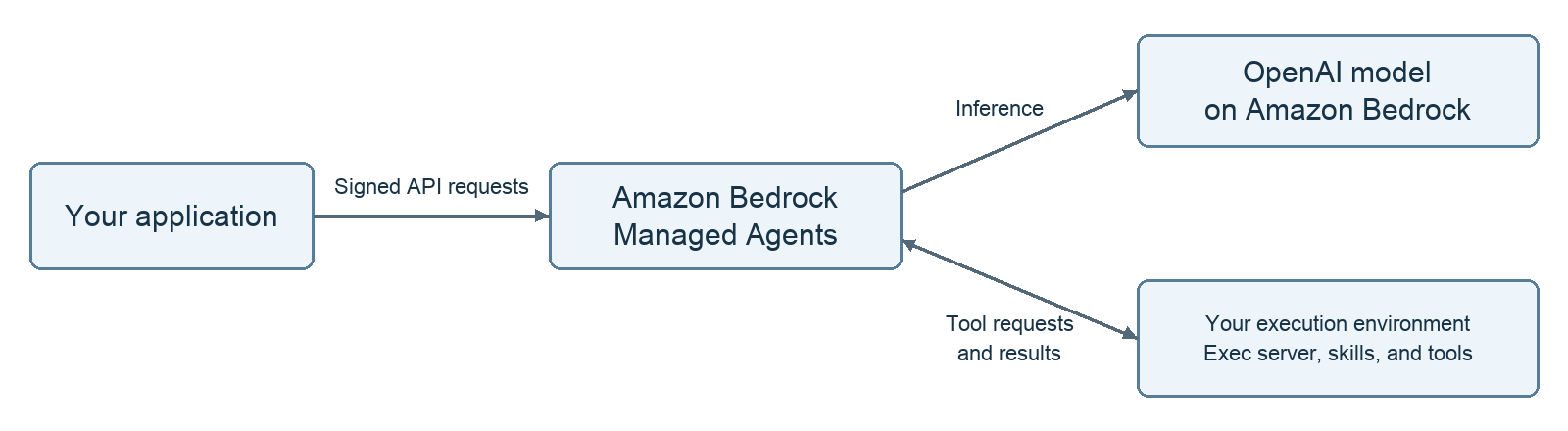
Last week, we announced a public preview of Amazon Bedrock Managed Agents powered by OpenAI, built on a customized version of OpenAI’s Agents API engineered to be AWS-native and integrated with AWS resources. You can now build agents optimized for OpenAI models that run entirely inside AWS with the identities, permissions, and governance controls you already use.
You can choose an execution environment: self-hosted compute to use an existing development machine, container, or compute environment or Amazon Bedrock AgentCore Runtime, for managed runtime sessions and configurable storage in your AWS account. To learn more, visit the Amazon Bedrock documentation.
In addition, we are adding new frontier models on Amazon Bedrock to expand your model choices:
OpenAI GPT-6.1 Sol: An upgrade to GPT-6 Sol, GPT-6.1 Sol delivers exceptionally strong performance on agentic coding, computer use, and professional work. According to OpenAI, it approaches GPT-6 Astra across demanding evaluations at roughly one-fifth of the cost, giving developers more room to build and run capable agents at scale. To learn more, visit the GPT-6.1 Sol model card.
OpenAI GPT-6 Astra UltraFast mode: Ultrafast is a premium speed tier for GPT-6 Astra, built for workloads where speed matters most. According to OpenAI, Ultrafast delivers up to 6x faster inference in the API, with up to 300 tokens per second. The Amazon Bedrock inference engine delivers the performance, security, and reliability required for production workloads. To learn more, visit the GPT-6 Astra model card.
Anthropic Claude Sonnet 5.5: Claude Sonnet 5.5 is a smarter, more efficient Sonnet and a step up from Sonnet 5, making it a natural upgrade for teams already building on Sonnet. It’s stronger for coding, completing well-scoped tasks as part of a larger coding strategy such as building and fixing features with Claude in the same session or verifying output against requirements. To learn more, visit the Claude Sonnet 5.5 model card.
SpaceXAI Grok 4.7: Grok 4.7 builds on Grok 4.6 with better mixed-document handling, more dependable repo-scale coding with planning and error recovery, and enhanced browser-use agents for form fills and portal navigation. To learn more, visit the Grok 4.7 model card.
Last week’s launches
Here are some launches that got my attention:
AWS Well-Architected Agent (preview): You can use an AI-powered agent service that analyzes your AWS environment to deliver targeted, contextual recommendations for improving your applications’ cost, security, performance, and resilience. The agent analyzes your infrastructure, understands your unique business goals, and delivers contextual recommendations.
Amazon S3 Tables support all Apache Iceberg V3 data types: Amazon S3 Tables add support for geometry, geography, unknown, and nanosecond timestamp data types, along with column default values, as defined in the Iceberg V3 specification. You can now store geospatial coordinates and nanosecond-precision event times natively instead of encoding them in strings or integers.
For a full list of AWS announcements, be sure to keep an eye on the What’s New with AWS page.
AWS service availability updates
When the availability of an AWS service or feature changes, we provide customers guidance in AWS Product Lifecycle Changes on available alternatives and support for migration so that disruptions to your operations are minimized. The following lifecycle changes were updated on September 29, 2026.
Services moving to Maintenance (no longer accessible to new customers starting October 29, 2026):
Services reaching End of Support (as of September 29, 2026):
Amazon Mechanical Turk
We understand that changes in availability can impact your operations. For specific guidance, consult the relevant service documentation or contact AWS Support.
Other AWS news
Here are some additional projects and news items you may find interesting:
Introducing Kiro workflows: Kiro workflows enable you to carry out complex tasks from start to finish with multiple agents and less supervision. We’ve been building Kiro itself with workflows, including the new cloud configuration, cloud sessions, and most of the workflow experience.
Introducing Strands Decider: Strands Decider is one of a new class of decision models or system one models, a type of model that has been gaining significant attention since TypeSafe AI’s launch of Jev earlier this month. Strands Decider 2B is a small, open source, decision model optimized for fast experimentation, local development, and innovation.
New FDE pathways for AWS Partners: On June 30, AWS announced the Forward Deployed Engineering (FDE) organization, backed by a $1 billion investment, and extended this hands-on delivery approach to AWS Partners through the Partner-Led FDE motion. Now, AWS Partners have a structured way to build and validate that depth with three new Partner FDE pathways and credentials that recognize the applied proficiency required to deliver production agentic AI.
For a full list of AWS blog posts, be sure to keep an eye on the AWS Blogs page.
Patch review has long been one of the limiting constraints for the kernel
project (and most others); there just aren’t enough people to properly
review all of the code that is submitted for inclusion. The Sashiko
system, which uses a large language model (LLM) to generate reviews
automatically, offers the prospect of some relief, and has already become
an important part of the kernel’s development process. At the 2026 edition
of Kernel Recipes, Roman
Gushchin, the maintainer of Sashiko, provided an overview of how
the system works and what is being done to improve it.
Version
3.0 of the MusicBrainz Picard
tag editor has been released. “This release brings many changes, including an
upgrade to Qt6, a completely new plugin system, several improvements to the user
interface, cover art processing, [International Standard Recording
Code (ISRC)] submission and many more.”
A year ago, many companies were cutting intern and new-graduate hiring. We went the other way. We announced a goal to hire as many as 1,111 interns in 2026, a number that’s a nod to 1.1.1.1, our public DNS resolver.
The bet was that AI makes early-career talent more valuable and able to make an impact faster. The best AI tools help people learn a system faster, try more ideas, and take on harder problems. They don’t supply the energy, curiosity and fresh eyes a new person brings to a team.
A year in, and our interns are shipping to our internal teams and to millions of customers.
If you’re reading this on the Cloudflare Blog, you’re already using some of their work. The blog runs on EmDash, and EmDash’s second maintainer started at Cloudflare as an intern this past summer.
A new generation of builders
We’re still working toward 1,111. So far, we’ve hosted 750 internships across 48 teams in nine offices: Austin, San Francisco, London, Lisbon, New York, Singapore, Bengaluru, Washington DC, and Sydney. And we’re still hiring.
From their first day, interns joined active teams and worked on real problems. Each was expected to leave something behind: a shipped product improvement, a better process, a new piece of infrastructure, or an insight that changes how a team approaches its work.
That work reached far beyond engineering. An internal audit intern built an AI-assisted pipeline to automate ISO compliance control testing and documentation. A product manager intern worked on an API, dashboard, and migration tooling to modernize credit management for our Startup Program. A people team software engineering intern improved background-verification workflows for new hires. A customer support intern explored ways to use AI to trigger troubleshooting commands from case descriptions.
AI-native interns, real-world results
AI was a key theme through the whole program, but it wasn’t a shortcut around learning or accountability. Interns used AI to understand unfamiliar codebases and systems, compare product requirements with implementation, prototype ideas, automate repetitive work, and accelerate the path from a question to a working solution. Managers and mentors remained essential in setting direction, reviewing decisions, and ensuring that what shipped met Cloudflare’s standards.
For many interns, AI moved the starting line. They could map a new project in days instead of weeks, create a working scaffold quickly, and spend more time on the hard questions: What should we build? Who will use it? How do we know it is correct? What happens when it reaches production?
One intern put it more bluntly: “How did previous interns ship anything in 12 weeks without AI?”
Interns ship at Cloudflare
Last year’s announcement had a section with that title. This year, the interns wrote the posts:
More cache from the same hardware. RAM and disk prices have climbed sharply over the past year, so our intern Aashi asked whether Cloudflare could get more cache capacity out of the servers it already has. Aashi built Cache Transcoding, which compresses eligible assets with Zstandard inside our primary proxy before they’re written to disk. In initial testing, it shrank them to a third of their original on-disk size on average. That points toward petabytes of effective cache capacity and less data moving between our data centers.
The CMS behind this blog. Noah joined as an intern and became EmDash’s second maintainer, contributing changes across the media library, content editor, and admin interface. EmDash 1.0 shipped during Birthday Week.
Getting ready for post-quantum. Cloudflare is targeting 2029 for post-quantum security, and you can’t migrate what you can’t see. Tiago helped build CryptoLabe, an internal AI tool that finds cryptography across our codebase and maps what depends on it. Sophie helped bring per-connection post-quantum visibility to Logpush, Log Explorer, and HTTP Traffic Analytics, so customers can check their own progress too.
Fixing the Internet’s plumbing. Some intern work goes beyond our products. Iliana measured how often networks rewrite BGP’s ORIGIN attribute to pull traffic their way, and found it on roughly 70% of observed paths. Then she publicly advocated for taking ORIGIN out of route selection altogether. She also tracked the adoption of RFC 9234, which lets routers reject route leaks on their own. Helping build a better Internet includes work like this: measuring a problem no single network owns, publishing the data, and proposing a fix.
Our interns didn't just help with Birthday Week, they shipped impactful work! Several of this year's Birthday Week launches included intern-authored and intern-engineered work:
An internship is also about the people you meet. Across our offices, interns shared meals, volunteered together, and made friends. Our CEO, Matthew Prince, hosted dinners with interns in offices around the world to hear directly about what they were working on and learning.
Executives also joined Q&A sessions where interns could ask candid questions about Cloudflare, strategy, technology, and careers. These sessions complemented the day-to-day support of managers and mentors, and gave interns a view of how the whole company works and where it’s going.
What comes next
We’ll keep growing the program next year, with a new cohort of interns, more teams taking part, and more learning about how early career people do their best work with AI and with the people around them.
And many of this year’s interns are coming back to Cloudflare full-time. A good summer is nice, but the outcome we want is a career and a new generation of people helping build a better Internet.
If you’re a student or early-career technologist, and you want your first project to ship to millions of people, apply to our internship program. We’ll keep opening up roles throughout the year.
We celebrated our 16th birthday last week by sharing how we’re building a better Internet for today’s world. As Matthew and Michelle reflected in this year’s Founders’ Letter, this year saw some of the most consequential changes in the history of the Internet.
For the first time, automated traffic surpassed human activity. AI is empowering people to build like never before, leading the Internet to grow massively in scale and unlocking more ambition and creativity. As we witnessed the influence that agent-driven recommendations have on consumer choices, we identified the need for a new approach that creates space for new businesses to succeed.
Each day of Birthday Week explored a different way we are helping to build the future of the Internet. We began on Monday by strengthening our commitment to open source. Tuesday focused on application security and the post-quantum transition. On Wednesday, we explored new economic models for the agentic Internet. Thursday, we expanded the Developer Platform with new tools for data analysis, storage, AI, and agent development. Finally, we closed out the week by launching features that make Cloudflare faster, easier to operate, and more accessible to everyone. As a special Birthday Week follow-up, we shared an update on our intern program, one year after announcing our goal to hire 1,111 interns. Interns directly contributed to many of the projects launched this week, including EmDash, post-quantum visibility, CryptoLabe, and Protected Quick Tunnels.
We shipped 46 announcements this week. In case you missed any, here’s the full list of everything we announced during Birthday Week 2026.
Monday, September 28 – Commitment to open source
With the announcement of our new CLI, which we released alongside the pipeline we use to generate it and our SDKs and docs, we shared how we’re building to support agents and developers as they use Cloudflare — and supporting the projects that you rely on, too.
The new cf CLI mirrors the Cloudflare API, uses JSON-first output and typed configuration, and gives people and agents one consistent command-line interface.
Since joining Cloudflare, VoidZero has delivered more than 80 releases across the Vite ecosystem, and its previously commercial Void platform will become fully open source.
Experimental Emscripten target support lets developers bring more native Rust libraries and applications, including progress toward Tokio support, to Workers.
The Cold Start gives five early-stage companies the opportunity to pitch live at Cloudflare Connect and compete for resources to help them grow.
Tuesday, September 29 – Helping secure the agentic Internet
Technological progress is rapidly changing how we think about application security. We announced our intention to become a certificate authority, as well as how we’re preparing foundational Internet cryptography for the post-quantum era and adapting application security to counter AI-driven attacks.
Twelve years after launching Universal SSL, Cloudflare announced its intention to become a public certificate authority (CA) and add resilience to free, automated certificate issuance.
Our planned CA will issue free Merkle Tree Certificates designed to make post-quantum authentication practical without imposing large certificate and handshake costs.
Cloudflare helped develop an IETF extension that authenticates the full IKEv2 transcript and prevents attackers from downgrading post-quantum IPsec tunnels.
HTTP Analytics, Log Explorer, and Logpush now show whether requests negotiated post-quantum key exchange, giving customers evidence they can inspect and report.
Application Profiles learns the expected structure of HTTP requests so customers can identify deviations and enforce what valid application traffic should look like.
An adaptive AI red-team system found WAF detection gaps across six attack categories, helping us improve normalization and managed rules for customers.
Threat Signals turns open-source reporting into structured indicators and connects the context to WAF rules, while the Threat Events Platform expands to every account.
Our application-security framework connects discovery, governance, runtime protection, investigation, and response in a continuous learning loop.
Wednesday, September 30 – Powering the agent economy
With our announcements of Pay Per Use and the release of our Monetization Gateway in beta, we shared how we’re building support for a new economic model that empowers creators to monetize their content and services.
Containers now has faster startup, flexible image and instance selection, new scheduling controls, and filesystem snapshots for persistent agent workspaces.
A new domain-search experience and expanded Registrar APIs make it easier for both people and agents to search, register, transfer, and manage domains.
Initiatives including Project Galileo, the Athenian Project, and Cloudflare for Campaigns have now delivered more than $100 million in donated services.
Thursday, October 1 – Bringing more of the developer stack to Cloudflare
We expanded what is possible to achieve on Cloudflare’s platform with the general availability launch of Cloudflare Basin, our data analytics platform, the launch of K2, a durable serverless event stream, and the announcement of our new contest — inviting developers to build a Git platform designed for agentic development.
Basin is now generally available, giving developers a serverless platform built on Apache Iceberg and R2 for ingesting, managing, and querying large datasets.
Workers adds opt-in native Web Crypto support for ML-KEM and ML-DSA, giving developers post-quantum primitives without bundling their own implementations.
Workers KV Instant delivers sub-two-millisecond p99 reads and fast global replication across more than 300 locations using the familiar Workers KV API.
Clef and Clef-flash are open-source decision models for fast classification and agent workflows, accompanied by a platform for reinforcement-learning fine-tuning.
Friday, October 2 – Delivering a faster, simpler Internet for everyone
We wrapped up the week with major updates to Cloudflare Observability, alongside adding Cloudflare Traces, network performance improvements that make Cloudflare faster, and an announcement on how we’re supporting civil society organizations.
Cloudflare Traces provides request-level visibility across security rules, transformations, cache, Workers, services, and origins without requiring an agent or SDK.
One year after our pledge, Logpush, multi-account governance, higher platform limits, and other capabilities are available to more customers across plans.
Account Abuse Protection uses stateful analysis and privacy-preserving Hashed User IDs to help teams investigate credential stuffing and fake-account creation.
Quick Tunnels now support email authentication, letting developers share a local application with selected people or domains without requiring Cloudflare accounts.
AI Gateway’s Web Search API brings current web context from multiple providers into model calls through REST APIs, Workers bindings, or customer-managed keys.
Streamline is an open-source example for building continuous video pipelines by combining Workers, Durable Objects, and a containerized media engine.
Building the Internet’s next chapter together
Across this week’s announcements, we kept returning to a consistent theme: the Internet should continue to open up more opportunities for people to create, contribute, and succeed. That means open tools developers can shape, security that keeps pace with new threats, a fairer exchange between agents and the people whose work they use, and infrastructure designed for the agentic Internet.
For 16 years, we have been building alongside developers, creators, researchers, customers, partners, and open-source communities. Your ideas, feedback, and willingness to challenge us have shaped Cloudflare, and that collaboration matters now more than ever.
Two Burp Suite extensions that group responses by content: Response Overview, a BApp with a threshold you set, and Colonel Clustered, which picks its own.
To provide the best experiences, we use technologies like cookies to store and/or access device information. Consenting to these technologies will allow us to process data such as browsing behavior or unique IDs on this site. Not consenting or withdrawing consent, may adversely affect certain features and functions.
Functional
Always active
The technical storage or access is strictly necessary for the legitimate purpose of enabling the use of a specific service explicitly requested by the subscriber or user, or for the sole purpose of carrying out the transmission of a communication over an electronic communications network.
Preferences
The technical storage or access is necessary for the legitimate purpose of storing preferences that are not requested by the subscriber or user.
Statistics
The technical storage or access that is used exclusively for statistical purposes.The technical storage or access that is used exclusively for anonymous statistical purposes. Without a subpoena, voluntary compliance on the part of your Internet Service Provider, or additional records from a third party, information stored or retrieved for this purpose alone cannot usually be used to identify you.
Marketing
The technical storage or access is required to create user profiles to send advertising, or to track the user on a website or across several websites for similar marketing purposes.
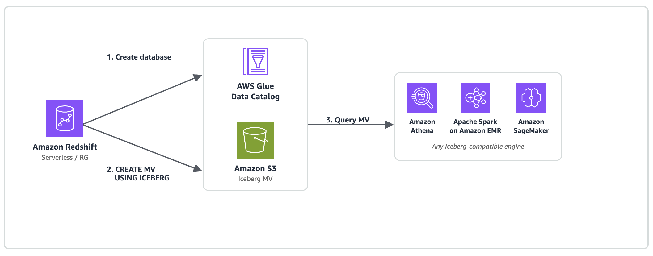


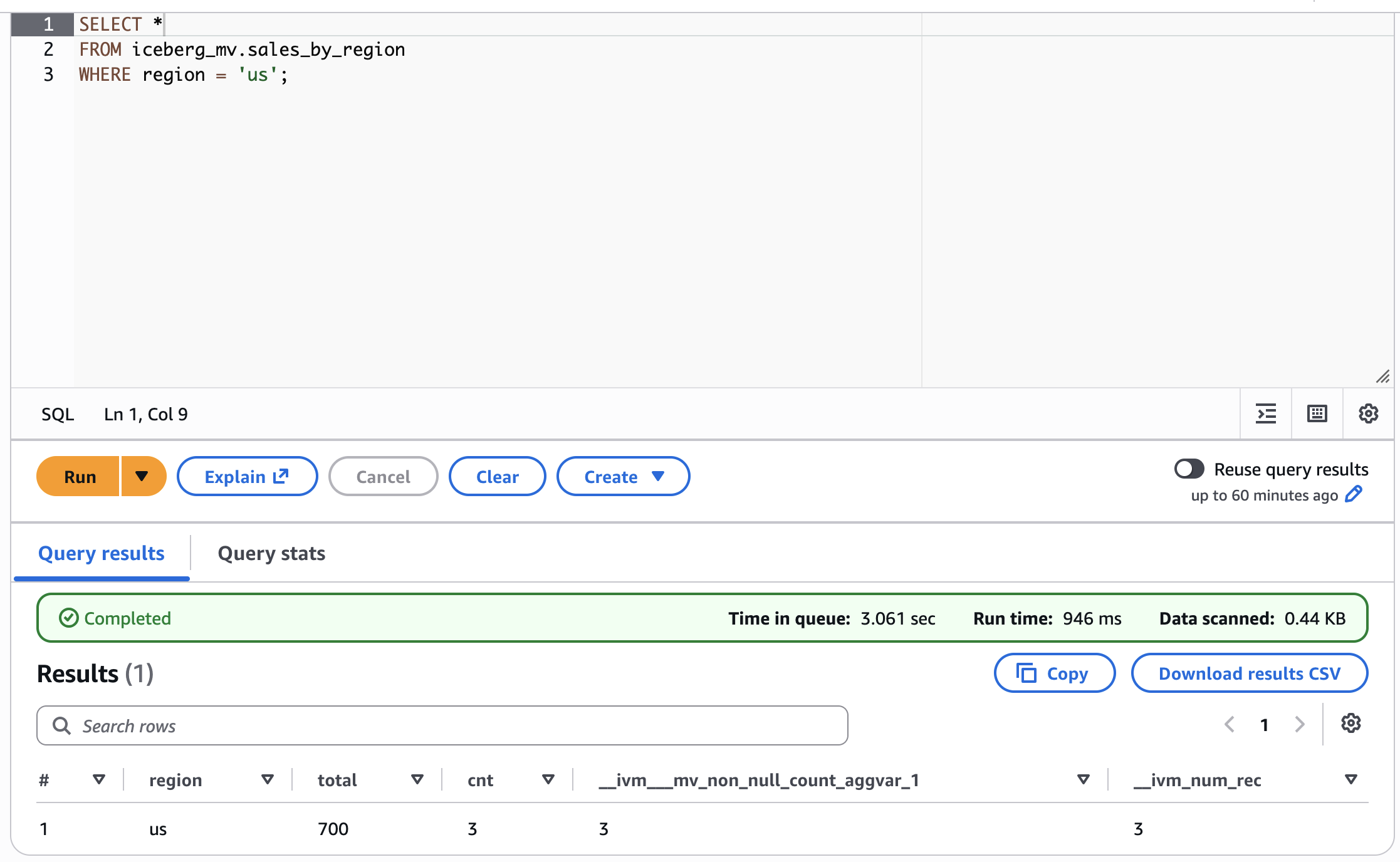
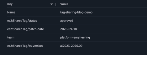
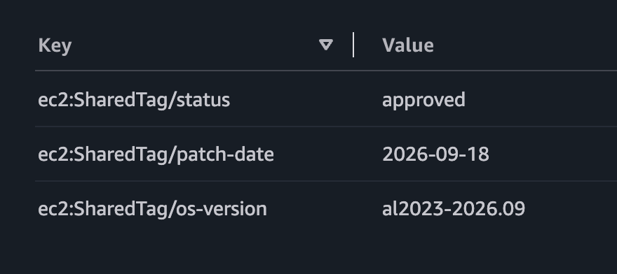
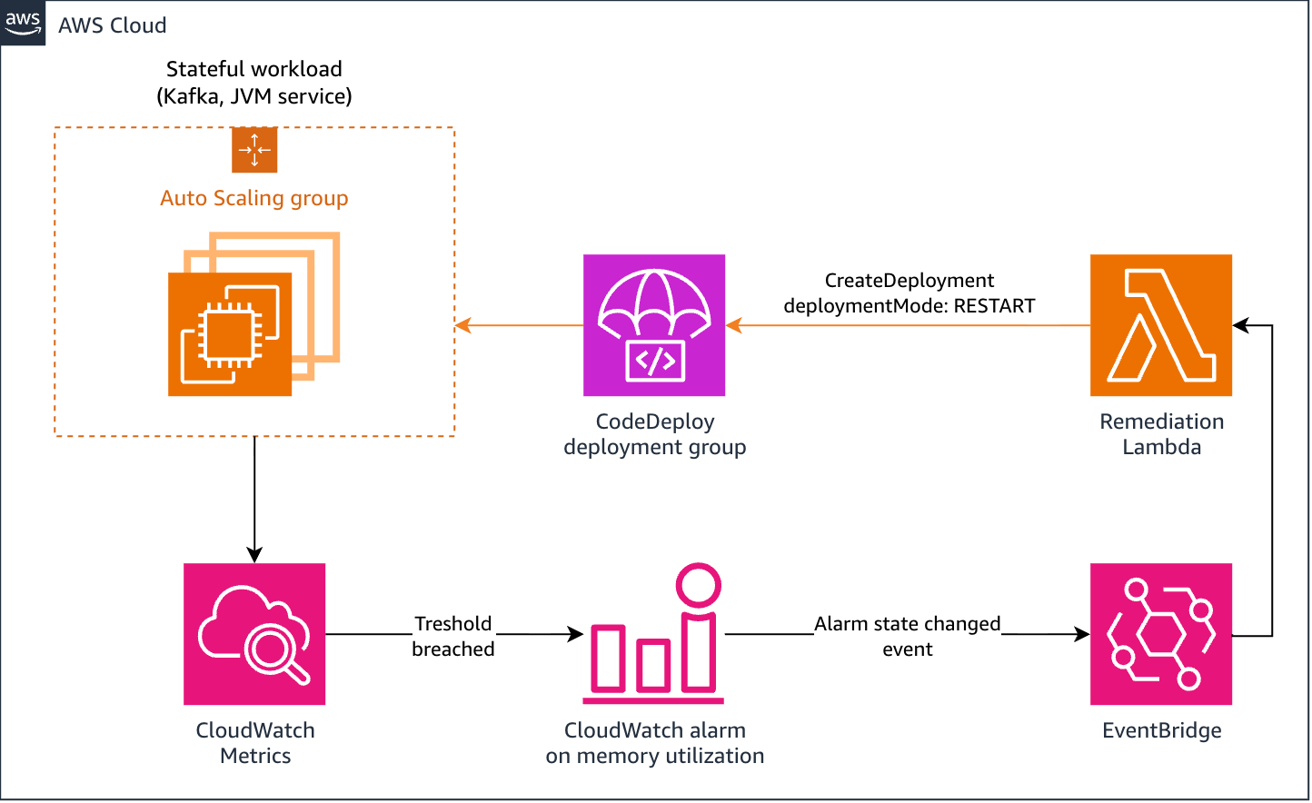
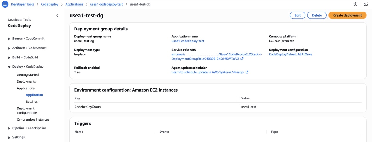
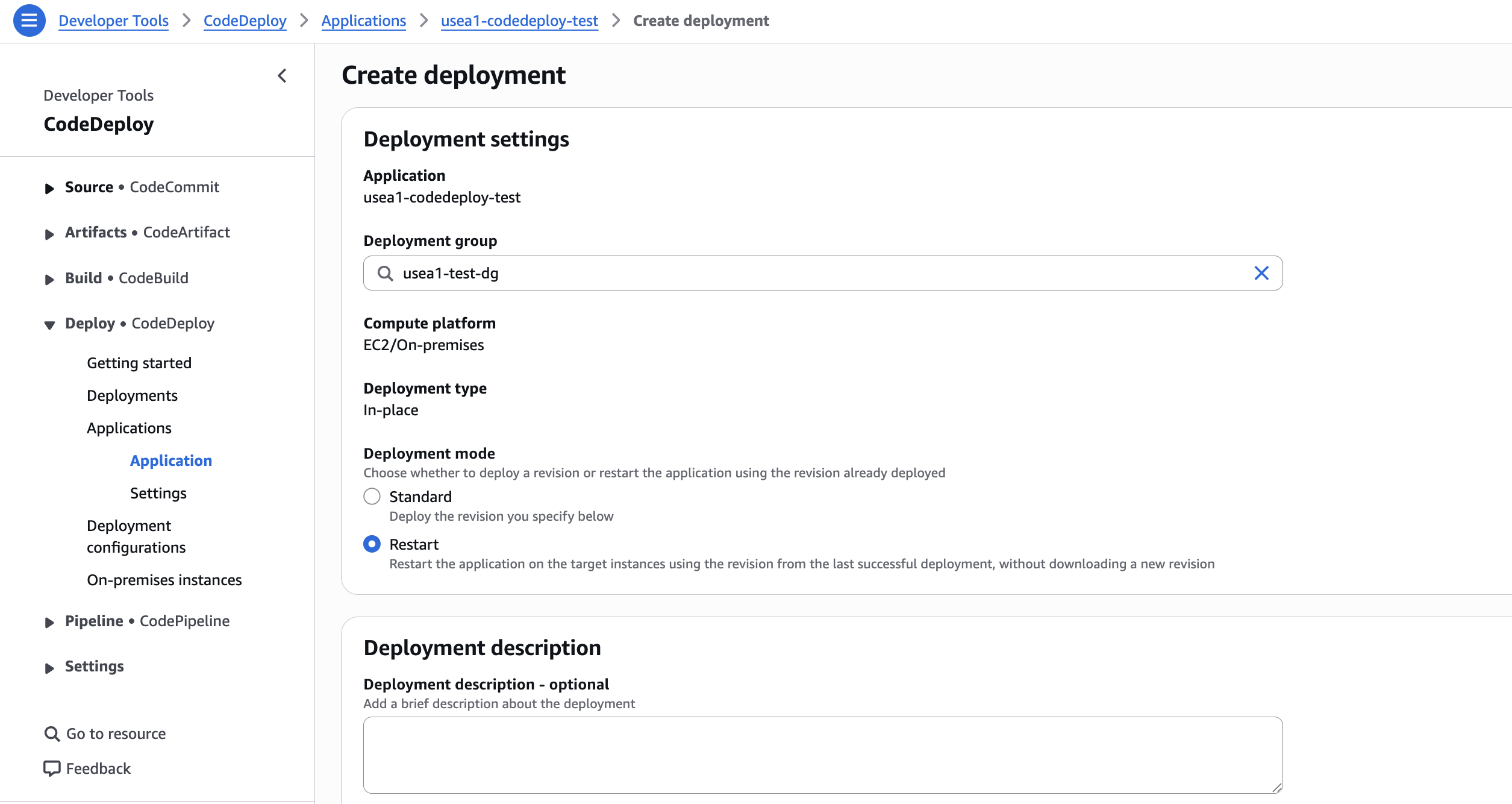
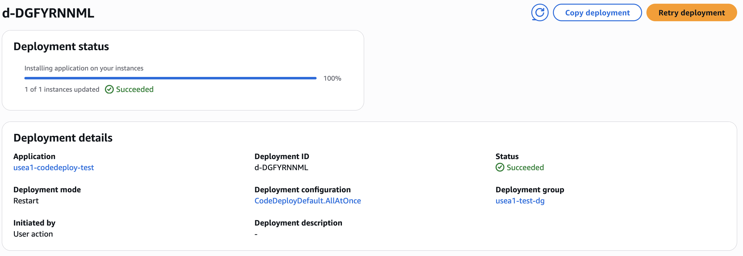
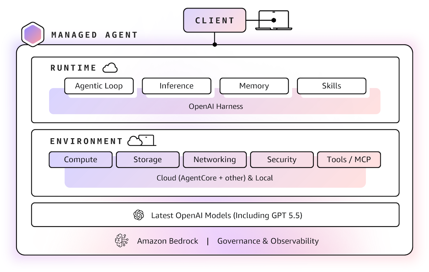 You can choose an execution environment: self-hosted compute to use an existing development machine, container, or compute environment or Amazon Bedrock AgentCore Runtime, for managed runtime sessions and configurable storage in your AWS account. To learn more, visit the