The GNU awk text-processing utility, gawk has released version
5.3.0. The main new features add compatibility with “The One True Awk” (also known
as “BWK awk”); version 5.3.0 adds CSV (comma-separated values) parsing and
the ability to use \u escape sequences for Unicode code points.
Read on for other changes in the release.
The 6.5.10 and 6.1.61 stable kernels have been released. As
usual, they contain important fixes throughout the kernel tree; users of
those series should upgrade.
Security updates have been issued by Gentoo (Netatalk), Oracle (firefox), Red Hat (.NET 6.0, .NET 6.0, .NET 7.0, binutils, and qemu-kvm), SUSE (gcc13, tomcat, and xorg-x11-server), and Ubuntu (axis, libvpx, linux-starfive, thunderbird, and xrdp).
For companies where security administration and ownership are distributed across a single organization in AWS Organizations, it’s important to have a mechanism for securely sharing and visualizing security data. This can be achieved by enriching data within Security Lake with organizational unit (OU) structure and account tags and using AWS Lake Formation to securely share data across your organization on a per-OU basis. Users can then analyze and visualize security data of only those AWS accounts in the OU that they have been granted access to. Enriching the data enables users to effectively filter information using business-specific criteria, minimizing distractions and enabling them to concentrate on key priorities.
Distributed security ownership
It’s not unusual to find security ownership distributed across an organization in AWS Organizations. Take for example a parent company with legal entities operating under it, which are responsible for the security posture of the AWS accounts within their lines of business. Not only is each entity accountable for managing and reporting on security within its area, it must not be able to view the security data of other entities within the same organization.
In this post, we discuss a common example of distributing dashboards on a per-OU basis for visualizing security posture measured by the AWS Foundational Security Best Practices (FSBP) standard as part of AWS Security Hub. In this post, you learn how to use a simple tool published on AWS Samples to extract OU and account tags from your organization and automatically create row-level security policies to share Security Lake data to AWS accounts you specify. At the end, you will have an aggregated dataset of Security Hub findings enriched with AWS account metadata that you can use as a basis for building QuickSight dashboards.
Although this post focuses on sharing Security Hub data through Security Lake, the same steps can be performed to share any data—including Security Hub findings in Amazon S3—according to OU. You need to ensure any tables you want to share contain an AWS account ID column and that the tables are managed by Lake Formation.
Prerequisites
This solution assumes you have:
Followed the previous posts in this series and understand how Security Lake, Lake Formation, and QuickSight work together.
Enabled Security Lake across your organization and have set up a delegated administrator account.
Configured Security Hub across your organization and have enabled the AWS FSBP standard.
Example organization
AnyCorp Inc, a fictional organization, wants to provide security compliance dashboards to its two subsidiaries, ExampleCorpEast and ExampleCorpWest, so that each only has access to data for their respective companies.
Each subsidiary has an OU under AnyCorp’s organization as well as multiple nested OUs for each line of business they operate. ExampleCorpEast and ExampleCorpWest have their own security teams and each operates a security tooling AWS account and uses QuickSight for visibility of security compliance data. AnyCorphas implemented Security Lake to centralize the collection and availability of security data across their organization and has enabled Security Hub and the AWS FSBP standard across every AWS account.
Figure 1: Overview of AnyCorp Inc OU structure and AWS accounts
Note: Although this post describes a fictional OU structure to demonstrate the grouping and distribution of security data, you can substitute your specific OU and AWS account details and achieve the same results.
Logical architecture
Figure 2: Logical overview of solution components
The solution includes the following core components:
An AWS Lambda function is deployed into the Security Lake delegated administrator account (Account A) and extracts AWS account metadata for grouping Security Lake data and manages secure sharing through Lake Formation.
Lake Formation implements row-level security using data filters to restrict access to Security Lake data to only records from AWS accounts in a particular OU. Lake Formation also manages the grants that allow consumer AWS accounts access to the filtered data.
Under Specify a template, choose Upload a template file and upload the file downloaded in the previous step. Then choose Next.
Enter RowLevelSecurityLakeStack as the stack name.
The table names used by Security Lake include AWS Region identifiers that you might need to change depending on the Region you’re using Security Lake in. Edit the following parameters if required and then choose Next.
MetadataDatabase: the name you want to give the metadata database.
Default: aws_account_metadata_db
SecurityLakeDB: the Security Lake database as registered by Security Lake.
On the Configure stack options screen, leave all other values as default and choose Next.
On the next screen, navigate to the bottom of the page and select the checkbox next to I acknowledge that AWS CloudFormation might create IAM resources. Choose Submit.
The solution takes about 5 minutes to deploy.
To deploy the solution using the AWS CDK, follow these steps:
Download the code from the row-level-security-lake GitHub repository, where you can also contribute to the sample code. The CDK initializes your environment and uploads the Lambda assets to Amazon S3. Then, deploy the solution to your account.
For a CDK deployment, you can edit the same Region identifier parameters discussed in the CloudFormation deployment option by editing the cdk.context.json file and changing the metadata_database, security_lake_db, and security_lake_table values if required.
While you’re authenticated in the Security Lake delegated administrator account, you can bootstrap the account and deploy the solution by running the following commands:
cdk bootstrap cdk deploy
Configuring the solution in the Security Lake delegated administrator account
After the solution has been successfully deployed, you can review the OUs discovered within your organization and specify which consumer AWS accounts (Account B) you want to share OU data with.
To specify AWS accounts to share OU security data with, follow these steps:
While in the Security Lake delegated administrator account (Account A), go to the Lake Formation console.
To view and update the metadata discovered by the Lambda function, you first must grant yourself access to the tables where it’s stored. Select the radio button for aws_account_metadata_db. Then, under the Action dropdown menu, select Grant.
Figure 3: Creating a grant for your IAM role
On the Grant data permissions page, under Principals, select the IAM users and roles dropdown and select the IAM role that you are currently logged in as.
Under LF-Tags or catalog resources, select the Tables dropdown and select All tables.
Figure 4: Choosing All Tables for the grant
Under Table permissions, select Select, Insert, and Alter. These permissions let you view and update the data in the tables.
Leave all other options as default and choose Grant.
Note: To use Athena for queries you must configure an S3 bucket to store query results. If this is the first time Athena is being used in your account, you will receive a message saying that you need to configure an S3 bucket. To do this, select the Edit settings button in the blue information notice and follow the instructions.
On the left side, select aws_account_metadata_db> as the Database. You will see aws_account_metadata and ou_groups >as tables within the database.
Figure 5: List of tables under the aws_accounts_metadata_db database
To view the OUs available within your organization, paste the following query into the Athena query editor window and choose Run.
SELECT * FROM "aws_account_metadata_db"."ou_groups"
Next, you must specify an AWS account you want to share an OU’s data with. Run the following SQL query in Athena and replace <AWS account Id> and <OU to assign> with values from your organization:
UPDATE "aws_account_metadata_db"."ou_groups"
SET consumer_aws_account_id = '<AWS account Id>'
WHERE ou = '<OU to assign>'
In the example organization, all ExampleCorpWest security data is shared with AWS account 123456789012 (Account B) using the following SQL query:
UPDATE "aws_account_metadata_db"."ou_groups"
SET consumer_aws_account_id = '123456789012'
WHERE ou = 'OU=root,OU=ExampleCorpWest'
Note: You must specify the full OU path beginning with OU=root.
Repeat this process for each OU you want to assign different AWS accounts to.
Note: You can only assign one AWS account ID to each OU group
You can confirm that changes have been applied by running the Athena query from Step 3 again.
SELECT * FROM "aws_account_metadata_db"."ou_groups"
You should see the AWS account ID you specified next to your OU.
Figure 6: Consumer AWS account listed against ExampleCorpWest OU
Invoke the Lambda function manually
By default, the Lambda function is scheduled to run hourly to monitor for changes to AWS account metadata and to update Lake Formation sharing permissions (grants) if needed. To perform the remaining steps in this post without having to wait for the hourly run, you must manually invoke the Lambda function.
To invoke the Lambda function manually, follow these steps:
Select the RowLevelSecurityLakeStack-* Lambda function.
Under Code source, choose Test.
The Lambda function doesn’t take any parameters. Enter rl-sec-lake-test as the Event name and leave all other options as the default. Choose Save.
Choose Test again. The Lambda function will take approximately 5 minutes to complete in an environment with less than 100 AWS accounts.
After the Lambda function has finished, you can review the data cell filters and grants that have been created in Lake Formation to securely share Security Lake data with your consumer AWS account (Account B).
To review the data filters and grants, follow these steps:
In the navigation pane, select Data filters under Data catalog to see a list of data cells filters that have been created for each OU that you assigned a consumer AWS account to. One filter is created per table. Each consumer AWS account is granted restricted access to the aws_account_metadata table and the aggregated Security Lake table.
Figure 7: Viewing data filters in Lake Formation
Select one of the filters in the list and choose Edit. Edit data filter displays information about the filter such as the database and table it’s applied to, as well as the Row filter expression that enforces row-level security to only return rows where the AWS account ID is in the OU it applies to. Choose Cancel to close the window.
Figure 8: Details of a data filter showing row filter expression
To see how the filters are used to grant restricted access to your tables, select Data lake permission under Permissions from navigation pane. In the search bar under Data permissions, enter the AWS account ID for your consumer AWS account (Account B) and press Enter. You will see a list of all the grants applied to that AWS account. Scroll to the right to see a column titled Resource that lists the names of the data cell filters you saw in the previous step.
Figure 9: Grants to the data consumer account for data filters
You can now move on to setting up the consumer AWS account.
Configuring QuickSight in the consumer AWS account (Account B)
Now that you’ve configured everything in the Security Lake delegated administrator account (Account A), you can configure QuickSight in the consumer account (Account B).
To confirm you can access shared tables, follow these steps:
Sign in to your consumer AWS account (also known as Account B).
Follow the same steps as outlined in this previous post (NEEDS 2ND POST IN SERIES LINK WHEN LIVE) to accept the AWS Resource Access Manager invitation, create a new database, and create resource links for the aws_account_metadata and amazon_security_lake_table_<region>_sh_findings_1_0 tables that have been shared with your consumer AWS account. Make sure you create resource links for both tables shared with the account. When done, return to this post and continue with step 3.
[Optional] After the resource links have been created, test that you’re able to query the data by selecting the radio button next to the aws_account_metadata resource link, select Actions, and then select View data under Table. This takes you to the Athena query editor where you can now run queries on the shared tables.
Figure 10: Selecting View data in Lake Formation to open Athena
Note: To use Athena for queries you must configure an S3 bucket to store query results. If this is the first time using Athena in your account, you will receive a message saying that you need to configure an S3 bucket. To do this, choose Edit settings in the blue information notice and follow the instructions.
In the Editor configuration, select AwsDataCatalog from the Data source options. The Database should be the database you created in the previous steps, for example security_lake_visualization. After selecting the database, copy the SQL query that follows and paste it into your Athena query editor, and choose Run. You will only see rows of account information from the OU you previously shared.
SELECT * FROM "security_lake_visualization"."aws_account_metadata"
Next, to enrich your Security Lake data with the AWS account metadata you need to create an Athena View that will join the datasets and filter the results to only return findings from the AWS Foundational Security Best Practices Standard. You can do this by copying the below query and running it in the Athena query editor.
CREATE OR REPLACE VIEW "security_hub_fsbps_joined_view" AS
WITH
  security_hub AS (
   SELECT *
   FROM
     "security_lake_visualization"."amazon_security_lake_table_ap_southeast_2_sh_findings_1_0"
   WHERE (metadata.product.feature.uid LIKE 'aws-foundational-security-best-practices%')
)
SELECT
  amm.*
, security_hub.*
FROM
  (security_hub
INNER JOIN "security_lake_visualization"."aws_account_metadata" amm ON (security_hub.cloud.account_uid = amm.id))
The SQL above performs a subquery to find only those findings in the Security Lake table that are from the AWS FSBP standard and then joins those rows with the aws_account_metadata table based on the AWS account ID. You can see it has created a new view listed under Views containing enriched security data that you can import as a dataset in QuickSight.
Figure 11: Additional view added to the security_lake_visualization database
Configuring QuickSight
To perform the initial steps to set up QuickSight in the consumer AWS account, you can follow the steps listed in the second post in this series. You must also provide the following grants to your QuickSight user:
To create a new dataset in QuickSight, follow these steps:
After your QuickSight user has the necessary permissions, open the QuickSight console and verify that you’re in same Region where Lake Formation is sharing the data.
Add your data by choosing Datasets from the navigation pane and then selecting New dataset. To create a new dataset from new data sources, select Athena.
Enter a data source name, for example security_lake_visualization, leave the Athena workgroup as [ primary ]. Then choose Create data source.
The next step is to select the tables to build your dashboards. On the Choose your table prompt, for Catalog, select AwsDataCatalog. For Database, select the database you created in the previous steps, for example security_lake_visualization. For Table, select the security_hub_fsbps_joined_view you created previously and choose Edit/Preview data.
Figure 12 – Choosing the joined dataset in QuickSight
You will be taken to a screen where you can preview the data in your dataset.
Figure 13: Previewing data in QuickSight
After you confirm you’re able to preview the data from the view, select the SPICE radio button in the bottom left of the screen and then choose PUBLISH & VISUALIZE.
You can now create analyses and dashboards from Security Hub AWS FSBP standard findings per OU and filter data based on business dimensions available to you through OU structure and account tags.
Figure 14: QuickSight dashboard showing only ExampleCorpWest OU data and incorporating business dimensions
Clean up the resources
To clean up the resources that you created for this example:
Sign in to the Security Lake delegated admin account and delete the CloudFormation stack by either:
Using the CloudFormation console to delete the stack, or
Using the AWS CDK to run cdk destroy in your terminal. Follow the instructions and enter y when prompted to delete the stack.
Remove any data filters you created by navigating to data filters within Lake Formation, selecting each one and choosing Delete.
Conclusion
In this final post of the series on visualizing Security Lake data with QuickSight, we introduced you to using a tool—available from AWS Samples—to extract OU structure and account metadata from your organization and use it to securely share Security Lake data on a per-OU basis across your organization. You learned how to enrich Security Lake data with account metadata and use it to create row-level security controls in Lake Formation. You were then able to address a common example of distributing security posture measured by the AWS Foundational Security Best Practices standard as part of AWS Security Hub.
If you have feedback about this post, submit comments in the Comments section below. If you have questions about this post, contact AWS Support.
Customers using Amazon Web Services (AWS) can use a range of native and third-party tools to build workloads based on their specific use cases. Logs and metrics are foundational components in building effective insights into the health of your IT environment. In a distributed and agile AWS environment, customers need a centralized and holistic solution to visualize the health and security posture of their infrastructure.
You can effectively categorize the members of the teams involved using the following roles:
Executive stakeholder: Owns and operates with their support staff and has total financial and risk accountability.
Data custodian: Aggregates related data sources while managing cost, access, and compliance.
Operator or analyst: Uses security tooling to monitor, assess, and respond to related events such as service disruptions.
In this blog post, we focus on the data custodian role. We show you how you can visualize metrics and logs centrally with Amazon QuickSight irrespective of the service or tool generating them. We use Amazon Simple Storage Service (Amazon S3) for storage, AWS Glue for cataloguing, and Amazon Athena for querying the data and creating structured query language (SQL) views for QuickSight to consume.
Target architecture
This post guides you towards building a target architecture in line with the AWS Well-Architected Framework. The tiered and multi-account target architecture, shown in Figure 1, uses account-level isolation to separate responsibilities across the various roles identified above and makes access management more defined and specific to those roles. The workload accounts generate the telemetry around the applications and infrastructure. The data custodian account is where the data lake is deployed and collects the telemetry. The operator account is where the queries and visualizations are created.
Throughout the post, I mention AWS services that reduce the operational overhead in one or more stages of the architecture.
Figure 1: Data visualization architecture
Ingestion
Irrespective of the technology choices, applications and infrastructure configurations should generate metrics and logs that report on resource health and security. The format of the logs depends on which tool and which part of the stack is generating the logs. For example, the format of log data generated by application code can capture bespoke and additional metadata deemed useful from a workload perspective as compared to access logs generated by proxies or load balancers. For more information on types of logs and effective logging strategies, see Logging strategies for security incident response.
Amazon S3 is a scalable, highly available, durable, and secure object storage that you will use as the storage layer. To build a solution that captures events agnostic of the source, you must forward data as a stream to the S3 bucket. Based on the architecture, there are multiple tools you can use to capture and stream data into S3 buckets. Some tools support integration with S3 and directly stream data to S3. Resources like servers and virtual machines need forwarding agents such as Amazon Kinesis Agent, Amazon CloudWatch agent, or Fluent Bit.
Amazon Kinesis Data Streams provides a scalable data streaming environment. Using on-demand capacity mode eliminates the need for capacity provisioning and capacity management for streaming workloads. For log data and metric collection, you should use on-demand capacity mode, because log data generation can be unpredictable depending on the requests that are being handled by the environment. Amazon Kinesis Data Firehose can convert the format of your input data from JSON to Apache Parquet before storing the data in Amazon S3. Parquet is naturally compressed, and using Parquet native partitioning and compression allows for faster queries compared to JSON formatted objects.
Amazon Security Lake is a fully managed security data lake service. You can use Security Lake to automatically centralize security data from AWS environments, SaaS providers, on-premises, and third-party sources into a purpose-built data lake that’s stored in your AWS account. Using Security Lake reduces the operational effort involved in building a scalable data lake, as the service automates the configuration and orchestration for the data lake with Lake Formation. Security Lake automatically transforms logs into a standard schema—the Open Cybersecurity Schema Framework (OCSF) — and parses them into a standard directory structure, which allows for faster queries. For more information, see How to visualize Amazon Security Lake findings with Amazon QuickSight.
You can start with basic queries and visualizations as described in Query logs in S3 with Athena and Create a QuickSight visualization. Depending on the nature and origin of the logs and metrics that you want to query, you can use the examples published in Running SQL queries using Amazon Athena. To build custom analytics, you can create views with Athena. Views in Athena are logical tables that you can use to query a subset of data. Views help you to hide complexity and minimize maintenance when querying large tables. Use views as a source for new datasets to build specific health analytics and dashboards.
You can also use Amazon QuickSight Q to get started on your analytics journey. Powered by machine learning, Q uses natural language processing to provide insights into the datasets. After the dataset is configured, you can use Q to give you suggestions for questions to ask about the data. Q understands business language and generates results based on relevant phrases detected in the questions. For more information, see Working with Amazon QuickSight Q topics.
Conclusion
Logs and metrics offer insights into the health of your applications and infrastructure. It’s essential to build visibility into the health of your IT environment so that you can understand what good health looks like and identify outliers in your data. These outliers can be used to identify thresholds and feed into your incident response workflow to help identify security issues. This post helps you build out a scalable centralized visualization environment irrespective of the source of log and metric data.
This post is part 1 of a series that helps you dive deeper into the security analytics use case. In part 2, How to visualize Amazon Security Lake findings with Amazon QuickSight, you will learn how you can use Security Lake to reduce the operational overhead involved in building a scalable data lake and centralizing log data from SaaS providers, on-premises, AWS, and third-party sources into a purpose-built data lake. You will also learn how you can integrate Athena with Security Lake and create visualizations with QuickSight of the data and events captured by Security Lake.
With the launch of Amazon Security Lake, it’s now simpler and more convenient to access security-related data in a single place. Security Lake automatically centralizes security data from cloud, on-premises, and custom sources into a purpose-built data lake stored in your account, and removes the overhead related to building and scaling your infrastructure as your data volumes increase. With Security Lake, you can get a more complete understanding of your security data across your entire organization. You can also improve the protection of your workloads, applications, and data.
Security Lake has adopted the Open Cybersecurity Schema Framework (OCSF), an open standard. With OCSF support, the service can normalize and combine security data from AWS and a broad range of enterprise security data sources. Using the native ingestion capabilities of the service to pull in AWS CloudTrail, Amazon Route 53, VPC Flow Logs, or AWS Security Hub findings, ingesting supported third-party partner findings, or ingesting your own security-related logs, Security Lake provides an environment in which you can correlate events and findings by using a broad range of tools from the AWS and APN partner community.
Many customers have already deployed and maintain a centralized logging solution using services such as Amazon OpenSearch Service or a third-party security information and event management (SIEM) tool, and often use business intelligence (BI) tools such as Amazon QuickSight to gain insights into their data. With Security Lake, you have the freedom to choose how you analyze this data. In some cases, it may be from a centralized team using OpenSearch or a SIEM tool, and in other cases it may be that you want the ability to give your teams access to QuickSight dashboards or provide specific teams access to a single data source with Amazon Athena.
Before you get started
To follow along with this post, you must have:
A basic understanding of Security Lake, Athena, and QuickSight
Security Lake already deployed and accepting data sources
An existing QuickSight deployment that can be used to visualize Security Lake data, or an account where you can sign up for QuickSight to create visualizations
Accessing data
Security Lake uses the concept of data subscribers when it comes to accessing your data. A subscriber consumes logs and events from Security Lake, and supports two types of access:
Data access — Subscribers can directly access Amazon Simple Storage Service (Amazon S3) objects and receive notifications of new objects through a subscription endpoint or by polling an Amazon Simple Queue Service (Amazon SQS) queue. This is the architecture typically used by tools such as OpenSearch Service and partner SIEM solutions.
Query access — Subscribers with query access can directly query AWS Lake Formation tables in your S3 bucket by using services like Athena. Although the primary query engine for Security Lake is Athena, you can also use other services that integrate with AWS Glue, such as Amazon Redshift Spectrum and Spark SQL.
In the sections that follow, we walk through how to configure cross-account sharing from Security Lake to visualize your data with QuickSight, and the associated Athena queries that are used. It’s a best practice to isolate log data from visualization workloads, and we recommend using a separate AWS account for QuickSight visualizations. A high-level overview of the architecture is shown in Figure 1.
Figure 1: Security Lake visualization architecture overview
In Figure 1, Security Lake data is being cataloged by AWS Glue in account A. This catalog is then shared to account B by using AWS Resource Access Manager. Users in account B are then able to directly query the cataloged Security Lake data using Athena, or get visualizations by accessing QuickSight dashboards that use Athena to query the data.
Configure a Security Lake subscriber
The following steps guide you through configuring a Security Lake subscriber using the delegated administrator account.
To configure a Security Lake subscriber
Sign in to the AWS Management Console and navigate to the Amazon Security Lake console in the Security Lake delegated administrator account. In this post, we’ll call this Account A.
Go to Subscribers and choose Create subscriber.
On the Subscriber details page, enter a Subscriber name. For example, cross-account-visualization.
For Log and event sources, select All log and event sources. For Data access method, select Lake Formation.
Add the Account ID for the AWS account that you’ll use for visualizations. In this post, we’ll call this Account B.
Security Lake creates a resource share in your visualizations account using AWS Resource Access Manager (AWS RAM). You can view the configuration of the subscriber from Security Lake by selecting the subscriber you just created from the main Subscribers page. It should look like Figure 2.
Figure 2: Subscriber configuration
Note: your configuration might be slightly different, based on what you’ve named your subscriber, the AWS Region you’re using, the logs being ingested, and the external ID that you created.
Configure Athena to visualize your data
Now that the subscriber is configured, you can move on to the next stage, where you configure Athena and QuickSight to visualize your data.
Note: In the following example, queries will be against Security Hub findings, using the Security Lake table in the ap-southeast-2 Region. If necessary, change the table name in your queries to match the Security Lake Region you use in the following configuration steps.
To configure Athena
Sign in to your QuickSight visualization account (Account B).
Navigate to the AWS Resource Access Manager (AWS RAM) console. You’ll see a Resource share invitation under Shared with me in the menu on the left-hand side of the screen. Choose Resource shares to go to the invitation.
Figure 3: RAM menu
On the Resource shares page, select the name of the resource share starting with LakeFormation-V3, and then choose Accept resource share. The Security Lake Glue catalog is now available to Account B to query.
For cross-account access, you should create a database to link the shared tables. Navigate to Lake Formation, and then under the Data catalog menu option, select Databases, then select Create database.
Enter a name, for example security_lake_visualization, and keep the defaults for all other settings. Choose Create database.
Figure 4: Create database
After you’ve created the database, you need to create resource links from the shared tables into the database. Select Tables under the Data catalog menu option. Select one of the tables shared by Security Lake by selecting the table’s name. You can identify the shared tables by looking for the ones that start with amazon_security_lake_table_.
From the Actions dropdown list, select Create resource link.
Figure 5: Creating a resource link
Enter the name for the resource link, for example amazon_security_lake_table_ap_southeast_2_sh_findings_1_0, and then select the security_lake_visualization database created in the previous steps.
Choose Create. After the links have been created, the names of the resource links will appear in italics in the list of tables.
You can now select the radio button next to the resource link, select Actions, and then select View data under Table. This takes you to the Athena query editor, where you can now run queries on the shared Security Lake tables.
Figure 6: Viewing data to query
To use Athena for queries, you must configure an S3 bucket to store query results. If this is the first time Athena is being used in your account, you’ll receive a message saying that you need to configure an S3 bucket. To do this, choose Edit settings in the information notice and follow the instructions.
In the Editor configuration, select AwsDataCatalog from the Data source options. The Database should be the database you created in the previous steps, for example security_lake_visualization.
After selecting the database, copy the query that follows and paste it into your Athena query editor, and then choose Run. This runs your first query to list 10 Security Hub findings:
Figure 7: Athena data query editor
SELECT * FROM
"AwsDataCatalog"."security_lake_visualization"."amazon_security_lake_table_ap_southeast_2_sh_findings_1_0" limit 10;
This queries Security Hub data in Security Lake from the Region you specified, and outputs the results in the Query results section on the page. For a list of example Security Lake specific queries, see the AWS Security Analytics Bootstrap project, where you can find example queries specific to each of the Security Lake natively ingested data sources.
To build advanced dashboards, you can create views using Athena. The following is an example of a view that lists 100 findings with failed checks sorted by created_time of the findings.
CREATE VIEW security_hub_new_failed_findings_by_created_time AS
SELECT
finding.title, cloud.account_uid, compliance.status, metadata.product.name
FROM "security_lake_visualization"."amazon_security_lake_table_ap_southeast_2_sh_findings_1_0"
WHERE compliance.status = 'FAILED'
ORDER BY finding.created_time
limit 100;
You can now query the view to list the first 10 rows using the following query.
SELECT * FROM
"security_lake_visualization"."security_hub_new_failed_findings_by_created_time" limit 10;
Create a QuickSight dataset
Now that you’ve done a sample query and created a view, you can use Athena as the data source to create a dataset in QuickSight.
To create a QuickSight dataset
Sign in to your QuickSight visualization account (also known as Account B), and open the QuickSight console.
When using cross-account configuration with AWS Glue Catalog, you also need to configure permissions on tables that are shared through Lake Formation. For a detailed deep dive, see Use Amazon Athena and Amazon QuickSight in a cross-account environment. For the use case highlighted in this post, use the following steps to grant access on the cross-account tables in the Glue Catalog.
In the AWS Lake Formation console, navigate to the Tables section and select the resource link for the table, for example amazon_security_lake_table_ap_southeast_2_sh_findings_1_0.
Select Actions. Under Permissions, select Grant on target.
For the LF-Tags or catalog resources section, use the default settings.
For Table permissions, choose Select for both Table Permissions and Grantable Permissions.
Choose Grant.
Figure 8: Granting permissions in Lake Formation
After permissions are in place, you can create datasets. You should also verify that you’re using QuickSight in the same Region where Lake Formation is sharing the data. The simplest way to determine your Region is to check the QuickSight URL in your web browser. The Region will be at the beginning of the URL. To change the Region, select the settings icon in the top right of the QuickSight screen and select the correct Region from the list of available Regions in the drop-down menu.
Select Datasets, and then select New dataset. Select Athena from the list of available data sources.
Enter a Data source name, for example security_lake_visualizations, and leave the Athena workgroup as [primary]. Then select Create data source.
Select the tables to build your dashboards. On the Choose your table prompt, for Catalog, select AwsDataCatalog. For Database, select the database you created in the previous steps, for example security_lake_visualization. For Table, select the table with the name starting with amazon_security_lake_table_. Choose Select.
Figure 9: Selecting the table for a new dataset
On the Finish dataset creation prompt, select Import to SPICE for quicker analytics. Choose Visualize.
In the left-hand menu in QuickSight, you can choose attributes from the data set to add analytics and widgets.
After you’re familiar with how to use QuickSight to visualize data from Security Lake, you can create additional datasets and add other widgets to create dashboards that are specific to your needs.
AWS pre-built QuickSight dashboards
So far, you’ve seen how to use Athena manually to query your data and how to use QuickSight to visualize it. AWS Professional Services is excited to announce the publication of the Data Visualization framework to help customers quickly visualize their data using QuickSight. The repository contains a combination of CDK tools and scripts that can be used to create the required AWS objects and deploy basic data sources, datasets, analysis, dashboards, and the required user groups to QuickSight with respect to Security Lake. The framework includes three pre-built dashboards based on the following personas.
Persona
Role description
Challenges
Goals
CISO/Executive Stakeholder
Owns and operates, with their support staff, all security-related activities within a business; total financial and risk accountability
Difficult to assess organizational aggregated security risk
Burdened by license costs of security tooling
Less agility in security programs due to mounting cost and complexity
Reduce risk
Reduce cost
Improve metrics (MTTD/MTTR and others)
Security Data Custodian
Aggregates all security-related data sources while managing cost, access, and compliance
Writes new custom extract, transform, and load (ETL) every time a new data source shows up; difficult to maintain
Manually provisions access for users to view security data
Constrained by cost and performance limitations in tools depending on licenses and hardware
Reduce overhead to integrate new data
Improve data governance
Streamline access
Security Operator/Analyst
Uses security tooling to monitor, assess, and respond to security-related events. Might perform incident response (IR), threat hunting, and other activities.
Moves between many security tools to answer questions about data
Lacks substantive automated analytics; manually processing and analyzing data
Can’t look historically due to limitations in tools (licensing, storage, scalability)
Reduce total number of tools
Increase observability
Decrease time to detect and respond
Decrease “alert fatigue”
After deploying through the CDK, you will have three pre-built dashboards configured and available to view. Once deployed, each of these dashboards can be customized according to your requirements. The Data Lake Executive dashboard provides a high-level overview of security findings, as shown in Figure 10.
Figure 10: Example QuickSight dashboard showing an overview of findings in Security Lake
The Security Lake custodian role will have visibility of security related data sources, as shown in Figure 11.
Figure 11: Security Lake custodian dashboard
And the Security Lake operator will have a view of security related events, as shown in Figure 12.
Figure 12: Security Operator dashboard
Conclusion
In this post, you learned about Security Lake, and how you can use Athena to query your data and QuickSight to gain visibility of your security findings stored within Security Lake. When using QuickSight to visualize your data, it’s important to remember that the data remains in your S3 bucket within your own environment. However, if you have other use cases or wish to use other analytics tools such as OpenSearch, Security Lake gives you the freedom to choose how you want to interact with your data.
We also introduced the Data Visualization framework that was created by AWS Professional Services. The framework uses the CDK to deploy a set of pre-built dashboards to help get you up and running quickly.
With the announcement of AWS AppFabric, we’re making it even simpler to ingest data directly into Security Lake from leading SaaS applications without building and managing custom code or point-to-point integrations, enabling quick visualization of your data from a single place, in a common format.
For additional information on using Athena to query Security Lake, have a look at the AWS Security Analytics Bootstrap project, where you can find queries specific to each of the Security Lake natively ingested data sources. If you want to learn more about how to configure and use QuickSight to visualize findings, we have hands-on QuickSight workshops to help you configure and build QuickSight dashboards for visualizing your data.
If you have feedback about this post, submit comments in the Comments section below. If you have questions about this post, contact AWS Support.
Want more AWS Security news? Follow us on Twitter.
You don’t always need the absolute fastest cloud storage—your performance requirements depend on your use case, business objectives, and security needs. But still, faster is usually better. And Backblaze just announced innovation on B2 Cloud Storage that delivers a lot more speed: most file uploads will now be up to 30% faster than AWS S3.
Today, I’m diving into all of the details of this performance improvement, how we did it, and what it means for you.
The TL:DR
The Results: Customers who rely on small file uploads (1MB or less) can expect to see 10–30% faster uploads on average based on our tests, all without any change to durability, availability, or pricing.
What Does This Mean for You?
All B2 Cloud Storage customers will benefit from these performance enhancements, especially those who use Backblaze B2 as a storage destination for data protection software. Small uploads of 1MB or less make up about 70% of all uploads to B2 Cloud Storage and are common for backup and archive workflows. Specific benefits of the performance upgrades include:
Secures data in offsite backup faster.
Frees up time for IT administrators to work on other projects.
Decreases congestion on network bandwidth.
Deduplicates data more efficiently.
Veeam® is dedicated to working alongside our partners to innovate and create a united front against cyber threats and attacks. The new performance improvements released by Backblaze for B2 Cloud Storage furthers our mission to provide radical resilience to our joint customers.
Today. The performance upgrades have been fully rolled out across Backblaze’s global data regions.
How We Did It
Prior to this work, when a customer uploaded a file to Backblaze B2, the data was written to multiple hard disk drives (HDDs). Those operations had to be completed before returning a response to the client. Now, we write the incoming data to the same HDDs and also, simultaneously, to a pool of solid state drives (SSDs) we call a “shard stash,” waiting only for the HDD writes to make it to the filesystems’ in-memory caches and the SSD writes to complete before returning a response. Once the writes to HDD are complete, we free up the space from the SSDs so it can be reused.
Since writing data to an SSD is much faster than writing to HDDs, the net result is faster uploads.
That’s just a brief summary; if you’re interested in the technical details (as well as the results of some rigorous testing), read on!
The Path to Performance Upgrades
As you might recall from many Drive Stats blog posts and webinars, Backblaze stores all customer data on HDDs, affectionately termed ‘spinning rust’ by some. We’ve historically reserved SSDs for Storage Pod (storage server) boot drives.
Until now.
That’s right—SSDs have entered the data storage chat. To achieve these performance improvements, we combined the performance of SSDs with the cost efficiency of HDDs. First, I’ll dig into a bit of history to add some context to how we went about the upgrades.
HDD vs. SSD
IBM shipped the first hard drive way back in 1957, so it’s fair to say that the HDD is a mature technology. Drive capacity and data rates have steadily increased over the decades while cost per byte has fallen dramatically. That first hard drive, the IBM RAMAC 350, had a total capacity of 3.75MB, and cost $34,500. Adjusting for inflation, that’s about $375,000, equating to $100,000 per MB, or $100 billion per TB, in 2023 dollars.
Today, the 16TB version of the Seagate Exos X16—an HDD widely deployed in the Backblaze B2 Storage Cloud—retails for around $260, $16.25 per TB. If it had the same cost per byte as the IBM RAMAC 250, it would sell for $1.6 trillion—around the current GDP of China!
SSDs, by contrast, have only been around since 1991, when SanDisk’s 20MB drive shipped in IBM ThinkPad laptops for an OEM price of about $1,000. Let’s consider a modern SSD: the 3.2TB Micron 7450 MAX. Retailing at around $360, the Micron SSD is priced at $112.50 per TB, nearly seven times as much as the Seagate HDD.
So, HDDs easily beat SSDs in terms of storage cost, but what about performance? Here are the numbers from the manufacturers’ data sheets:
Since HDD platters rotate at a constant rate, 7,200 RPM in this case, they can transfer more blocks per revolution at the outer edge of the disk than close to the middle—hence the two figures for the X16’s transfer rate.
The SSD is over 20 times as fast at sustained data transfer than the HDD, but look at the difference in random transfer rates! Even when the HDD is at its fastest, transferring blocks from the outer edge of the disk, the SSD is over 2,200 times faster reading data and nearly 900 times faster for writes.
This massive difference is due to the fact that, when reading data from random locations on the disk, the platters have to complete an average of 0.5 revolutions between blocks. At 7,200 rotations per minute (RPM), that means that the HDD spends about 4.2ms just spinning to the next block before it can even transfer data. In contrast, the SSD’s data sheet quotes its latency as just 80µs (that’s 0.08ms) for reads and 15µs (0.015ms) for writes, between 84 and 280 times faster than the spinning disk.
Let’s consider a real-world operation, say, writing 64kB of data. Assuming the HDD can write that data to sequential disk sectors, it will spin for an average of 4.2ms, then spend 0.25ms writing the data to the disk, for a total of 4.5ms. The SSD, in contrast, can write the data to any location instantaneously, taking just 27µs (0.027ms) to do so. This (somewhat theoretical) 167x speed advantage is the basis for the performance improvement.
Why did I choose a 64kB block? As we mentioned in a recent blog post focusing on cloud storage performance, in general, bigger files are better when it comes to the aggregate time required to upload a dataset. However, there may be other requirements that push for smaller files. Many backup applications split data into fixed size blocks for upload as files to cloud object storage. There is a trade-off in choosing the block size: larger blocks improve backup speed, but smaller blocks reduce the amount of storage required. In practice, backup blocks may be as small as 1MB or even 256kB. The 64kB blocks we used in the calculation above represent the shards that comprise a 1MB file.
The challenge facing our engineers was to take advantage of the speed of solid state storage to accelerate small file uploads without breaking the bank.
Improving Write Performance for Small Files
When a client application uploads a file to the Backblaze B2 Storage Cloud, a coordinator pod splits the file into 16 data shards, creates four additional parity shards, and writes the resulting 20 shards to 20 different HDDs, each in a different Pod.
Note: As HDD capacity increases, so does the time required to recover after a drive failure, so we periodically adjust the ratio between data shards and parity shards to maintain our eleven nines durability target. In the past, you’ve heard us talk about 17 + 3 as the ratio but we also run 16 + 4 and our very newest vaults use a 15 + 5 scheme.
Each Pod writes the incoming shard to its local filesystem; in practice, this means that the data is written to an in-memory cache and will be written to the physical disk at some point in the near future. Any requests for the file can be satisfied from the cache, but the data hasn’t actually been persistently stored yet.
We need to be absolutely certain that the shards have been written to disk before we return a “success” response to the client, so each Pod executes an fsync system call to transfer (“flush”) the shard data from system memory through the HDD’s write cache to the disk itself before returning its status to the coordinator. When the coordinator has received at least 19 successful responses, it returns a success response to the client. This ensures that, even if the entire data center was to lose power immediately after the upload, the data would be preserved.
As we explained above, for small blocks of data, the vast majority of the time spent writing the data to disk is spent waiting for the drive platter to spin to the correct location. Writing shards to SSD could result in a significant performance gain for small files, but what about that 7x cost difference?
Our engineers came up with a way to have our cake and eat it too by harnessing the speed of SSDs without a massive increase in cost. Now, upon receiving a file of 1MB or less, the coordinator splits it into shards as before, then simultaneously sends the shards to a set of 20 Pods and a separate pool of servers, each populated with 10 of the Micron SSDs described above—a “shard stash.” The shard stash servers easily win the “flush the data to disk” race and return their status to the coordinator in just a few milliseconds. Meanwhile, each HDD Pod writes its shard to the filesystem, queues up a task to flush the shard data to the disk, and returns an acknowledgement to the coordinator.
Once the coordinator has received replies establishing that at least 19 of the 20 Pods have written their shards to the filesystem, and at least 19 of the 20 shards have been flushed to the SSDs, it returns its response to the client. Again, if power was to fail at this point, the data has already been safely written to solid state storage.
We don’t want to leave the data on the SSDs any longer than we have to, so, each Pod, once it’s finished flushing its shard to disk, signals to the shard stash that it can purge its copy of the shard.
Real-World Performance Gains
As I mentioned above, that calculated 167x performance advantage of SSDs over HDDs is somewhat theoretical. In the real world, the time required to upload a file also depends on a number of other factors—proximity to the data center, network speed, and all of the software and hardware between the client application and the storage device, to name a few.
The first Backblaze region to receive the performance upgrade was U.S. East, located in Reston, Virginia. Over a 12-day period following the shard stash deployment there, the average time to upload a 256kB file was 118ms, while a 1MB file clocked in at 137ms. To replicate a typical customer environment, we ran the test application at our partner Vultr’s New Jersey data center, uploading data to Backblaze B2 across the public internet.
For comparison, we ran the same test against Amazon S3’s U.S. East (Northern Virginia) region, a.k.a. us-east-1, from the same machine in New Jersey. On average, uploading a 256kB file to S3 took 157ms, with a 1MB file taking 153ms.
So, comparing the Backblaze B2 U.S. East region to the Amazon S3 equivalent, we benchmarked the new, improved Backblaze B2 as 30% faster than S3 for 256kB files and 10% faster than S3 for 1MB files.
These low-level tests were confirmed when we timed Veeam Backup & Replication software backing up 1TB of virtual machines with 256k block sizes. Backing the server up to Amazon S3 took three hours and 12 minutes; we measured the same backup to Backblaze B2 at just two hours and 15 minutes, 40% faster than S3.
Test Methodology
We wrote a simple Python test app using the AWS SDK for Python (Boto3). Each test run involved timing 100 file uploads using the S3 PutObject API, with a 10ms delay between each upload. (FYI, the delay is not included in the measured time.) The test app used a single HTTPS connection across the test run, following best practice for API usage. We’ve been running the test on a VM in Vultr’s New Jersey region every six hours for the past few weeks against both our U.S. East region and its AWS neighbor. Latency to the Backblaze B2 API endpoint averaged 5.7ms, to the Amazon S3 API endpoint 7.8ms, as measured across 100 ping requests.
What’s Next?
At the time of writing, shard stash servers have been deployed to all of our data centers, across all of our regions. In fact, you might even have noticed small files uploading faster already. It’s important to note that this particular optimization is just one of a series of performance improvements that we’ve implemented, with more to come. It’s safe to say that all of our Backblaze B2 customers will enjoy faster uploads and downloads, no matter their storage workload.
Apple has warned leaders of the opposition government in India that their phones are being spied on:
Multiple top leaders of India’s opposition parties and several journalists have received a notification from Apple, saying that “Apple believes you are being targeted by state-sponsored attackers who are trying to remotely compromise the iPhone associated with your Apple ID ….”
For India to uphold fundamental rights, authorities must initiate an immediate independent inquiry, implement a ban on the use of rights-abusing commercial spyware, and make a commitment to reform the country’s surveillance laws. These latest warnings build on repeated instances of cyber intrusion and spyware usage, and highlights the surveillance impunity in India that continues to flourish despite the public outcry triggered by the 2019 Pegasus Project revelations.
We are pleased to announce a new AI-themed challenge for young people: the Experience AI Challenge invites and supports young people aged up to 18 to design and make their own AI applications. This is their chance to have a taste of getting creative with the powerful technology of machine learning. And equally exciting: every young creator will get feedback and encouragement from us at the Raspberry Pi Foundation.
As you may have heard, we recently launched a series of classroom lessons called Experience AI in partnership with Google DeepMind. The lesson materials make it easy for teachers of all subjects to teach their learners aged up to 18 about artificial intelligence and machine learning. Now the Experience AI Challenge gives young people the opportunity to develop their skills further and build their own AI applications.
Key information
Starts on 08 January 2024
Free to take part in
Designed for beginners, based on the tools Scratch and Machine Learning for Kids
Open for official submissions made by UK-based young people aged up to 18 and their mentors
Young people and their mentors around the world are welcome to access the Challenge resources and make AI projects
Tailored resources for young people and mentors to support you to take part
For the Experience AI Challenge, you and the young people you work with will learn how to make a machine learning (ML) classifier that organises data types such as audio, text, or images into different groupings that you specify.
The Challenge resources show young people the basic principles of using the tools and training ML models. Then they will use these new skills to create their own projects, and it’s a chance for their imaginations to run free. Here are some examples of projects your young tech creators could make:
An instrument classifier to identify the type of musical instrument being played in pieces of music
An animal sound identifier to determine which animal is making a particular sound
A voice command recogniser to detect voice commands like ‘stop’, ‘go’, ‘left’, and ‘right’
A photo classifier to identify what kind of food is shown in a photograph
All creators will receive expert feedback on their projects.
To make the Experience AI Challenge as familiar and accessible as possible for young people who may be new to coding, we designed it for beginners. We chose the free, easy-to-use, online tool Machine Learning for Kids for young people to train their machine learning models, and Scratch as the programming environment for creators to code their projects. If you haven’t used these tools before, don’t worry. The Challenge resources will provide all the support you need to get up to speed.
Training an ML model and creating a project with it teaches many skills beyond coding, including computational thinking, ethical programming, data literacy, and developing a broader understanding of the influence of AI on society.
The three Challenge stages
Our resources for creators and mentors walk you through the three stages of the Experience AI Challenge.
Stage 1: Explore and discover
The first stage of the Challenge is designed to ignite young people’s curiosity. Through our resources, mentors let participants explore the world of AI and ML and discover how these technologies are revolutionising industries like healthcare and entertainment.
Stage 2: Get hands-on
In the second stage, young people choose a data type and embark on a guided example project. They create a training dataset, train an ML model, and develop a Scratch application as the user interface for their model.
Stage 3: Design and create
In the final stage, mentors support young people to apply what they’ve learned to create their own ML project that addresses a problem they’re passionate about. They submit their projects to us online and receive feedback from our expert panel.
LWN.net is looking to hire a full-time writer/editor to help us keep the
news flowing and to expand our content in areas of interest to our readers.
We are certain that the person we need is out there somewhere, and are
counting on help from LWN readers to find them. Read on for details on who
we are looking for and how we see them fitting in here.
When you build on Amazon Web Services (AWS) across accounts, you might use an AWS Identity and Access Management (IAM) role to allow an authenticated identity from outside your account—such as an IAM entity or a user from an external identity provider—to access the resources in your account. IAM roles have two types of policies attached to them: a trust policy that allows access to an external entity, and a permissions policy that defines what actions the role can take. This blog post focuses on how to use AWS Identity and Access Management Access Analyzer cross-account access findings and IAM action last accessed information to refine the permissions policies of your IAM roles that have a trust policy.
IAM Access Analyzer helps you set, verify, and refine permissions. To learn more about how IAM Access Analyzer guides you toward least-privilege permissions, visit Using AWS IAM Access Analyzer. Action last accessed information helps you identify unused permissions and refine the access of your IAM roles to only the actions they use. IAM now provides action last accessed information for more than 140 services such as Amazon Kinesis Data Streams and Data Firehose, Amazon DynamoDB, and Amazon Simple Queue Service (Amazon SQS).
This blog post walks you through how to use IAM Access Analyzer and action last accessed to refine the required permissions for your IAM roles that have a trust policy, which allows entities outside of your account to assume a role and access your resources.
Use IAM roles to grant access to an external entity
You can create an IAM role that grants permissions for an entity outside your account to access the resources in your account. For example, if you’re an application developer, you might grant cross-account access to your AWS resources by using a role and attaching a trust policy to the role.
To allow an external entity access to your resources by using a role, you first create a role with a role trust policy to grant access to entities outside your account, and then grant permissions that specify which actions the role can take. The external entities can then assume the role in your account and access your resources based on the permissions you granted to the role. See Cross-account access using roles for more information.
You should restrict the access of roles that grant access outside of your account to just the permissions required to perform a specific task.
Use IAM Access Analyzer cross-account access findings to identify roles that grant access to external entities
When you use role trust policies to grant account access to entities outside your account, those entities can access and take the allowed actions on your resources. IAM Access Analyzer continuously monitors your account to identify the resources in your account that can be accessed from outside your account and helps you verify whether the access permissions meet your intent. For the example in this post, if you were to add a new trust policy to your ApplicationRole to grant permissions to an external account to access an application in your account, IAM Access Analyzer would let you know that ApplicationRole is accessible by entities from outside your account.
Use IAM action last accessed information to identify and remove unused permissions
After you’ve identified the IAM roles that grant access to entities outside your account, review what those roles can do and remove unused permissions. You can use action last accessed to show you the latest timestamp when your IAM role used an action, analyze its access permissions, and remove unused permissions.
Refine permissions for externally accessible roles by using IAM Access Analyzer cross-account access findings and action last accessed information
This example demonstrates how you can combine the information from IAM Access Analyzer cross-account access findings and IAM action last accessed information to identify roles that can be assumed from outside your account, review unused and unnecessary actions, and reduce the permissions available to external roles.
To view action last accessed information in the IAM console
Open the AWS Management Console and go to the IAM console, and then select Access analyzer in the navigation pane.
Review your findings on the IAM Access Analyzer tab.
Under Active findings, for Filter active findings, enter AWS::IAM::Role. The list of Active findings shows you the roles that can be accessed by entities outside your account.
Figure 1: Findings filtered by resource types
Under the Finding ID column, select a finding for a role (for example, ApplicationRole) that you want to review.
A new page for the Finding ID will appear. Choose the resource ARN link in the Resource field under the Details section.
Figure 2: Findings page
A new page for the role will appear. Select the Access Advisor tab to review the last accessed information of your services for this role. This tab displays the AWS services to which the role has permissions. Action last accessed reports the actions listed in the IAM action last accessed information services and actions. The tracking period for services is the last 400 days—fewer if your AWS Region began tracking within the last 400 days. Learn more about Where AWS tracks last accessed information.
Figure 3: Last accessed information of allowed services
In this exercise, we will use DynamoDB as an example. Under Allowed services, for Search, enter Amazon DynamoDB and under the Service column, choose Amazon DynamoDB. This will take you to a new section titled Allowed management actions for Amazon DynamoDB, which displays the action last accessed information of your role for DynamoDB. The Action column displays the action, the Last Accessed column displays the timestamp of when access was last attempted, and the Region accessed column displays in which region access was last attempted.
The Action column on the resulting Allowed management actions for Amazon DynamoDB section includes the actions to which the role has permissions, when the role last accessed each action, and the Region accessed. You can sort the actions by choosing the arrow next to Last accessed.
Figure 4: Action last accessed information for Amazon DynamoDB
Because you want to remove unused permissions, filter for all unused actions for the role by selecting Servicesnot accessed from the Last accessed dropdown list. This will show you the actions that haven’t been accessed during the tracking period.
Figure 5: Action last accessed information ordered by not accessed
To return to the service view, choose Back to Allowed services and then select the Permissions tab. Select the plus sign to the left of DynamoDBAccess to see the JSON of the customer managed policy.
Figure 6: The JSON code of the customer managed policy
Choose Next and then Save changes. Return to the Access Advisor tab to confirm that all the retained permissions have been used recently.
Conclusion
In this post, you learned how to use IAM Access Analyzer and action last accessed information to identify and refine permissions for externally accessible roles in your journey toward least privilege. You first used IAM Access Analyzer cross-account access findings to identify IAM roles that can be accessed from outside your account. You then used IAM action last accessed information to review the permissions those roles are using and to remove unused permissions.
If you have feedback about this post, submit comments in the Comments section below. If you have questions about this post, start a new thread on the AWS re:Post or contact AWS Support.
Tom Elkins, John Fenninger, Evan McCann, Matthew Smith, and Micah Young contributed attacker behavior insights to this blog.
Beginning Friday, October 27, Rapid7 Managed Detection and Response (MDR) identified suspected exploitation of Apache ActiveMQ CVE-2023-46604 in two different customer environments. In both instances, the adversary attempted to deploy ransomware binaries on target systems in an effort to ransom the victim organizations. Based on the ransom note and available evidence, we attribute the activity to the HelloKitty ransomware family, whose source code was leaked on a forum in early October. Rapid7 observed similar indicators of compromise across the affected customer environments, both of which were running outdated versions of Apache ActiveMQ.
CVE-2023-46604 is a remote code execution vulnerability in Apache ActiveMQ that allows a remote attacker with network access to a broker “to run arbitrary shell commands by manipulating serialized class types in the OpenWire protocol to cause the broker to instantiate any class on the classpath.” This is one of the more convoluted vulnerability descriptions we’ve seen, but the root cause of the issue is insecure deserialization.
Apache disclosed the vulnerability and released new versions of ActiveMQ on October 25, 2023. Proof-of-concept exploit code and vulnerability details are both publicly available. Rapid7’s vulnerability research team has tested the public PoC and confirmed that the behavior MDR observed in customer environments is similar to what we would expect from exploitation of CVE-2023-46604. Rapid7 research has a technical analysis of the vulnerability in AttackerKB.
Affected Products
According to Apache’s advisory, CVE-2023-46604 affects the following:
Apache ActiveMQ 5.18.0 before 5.18.3
Apache ActiveMQ 5.17.0 before 5.17.6
Apache ActiveMQ 5.16.0 before 5.16.7
Apache ActiveMQ before 5.15.16
Apache ActiveMQ Legacy OpenWire Module 5.18.0 before 5.18.3
Apache ActiveMQ Legacy OpenWire Module 5.17.0 before 5.17.6
Apache ActiveMQ Legacy OpenWire Module 5.16.0 before 5.16.7
Apache ActiveMQ Legacy OpenWire Module 5.8.0 before 5.15.16
Observed Attacker Behavior
During a successful exploitation of the vulnerability, Java.exe will contain the specific Apache application being targeted — in this case, D:\Program files\ActiveMQ\apache-activemq-5.15.3\bin\win64, which was observed as the parent process in both incidents. Post-exploitation, the adversary attempted to load remote binaries named M2.png and M4.png using MSIExec. The threat actor’s attempts at ransomware deployment were somewhat clumsy: In one of the incidents Rapid7 observed, there were more than half a dozen unsuccessful attempts to encrypt assets.
HelloKitty Ransomware Details
Rapid7 acquired the MSI files M4.png and M2.png from the domain 172.245.16[.]125 and analyzed them in a controlled environment. After analysis, Rapid7 observed that both MSI files contained a 32-bit .NET executable internally named dllloader. Within the .NET executable dllloader, Rapid7 found that the executable loads a Base64-encoded payload. We decoded the Base64-encoded payload and determined that it was a 32-bit .NET DLL named EncDLL.
The EncDLL binary contained functionality similar to that of ransomware — the DLL searches for specific processes and stops them from running. Rapid7 observed the DLL will encrypt specific file extensions using the RSACryptoServiceProvider function, appending encrypted files with the extension .locked. We also observed another function that provided information about which directories to avoid encrypting, a static variable assigned with the ransomware note, and a function that attempted communication to an HTTP server, 172.245.16[.]125.
The ransomware note indicated communications should occur through the email address service@hellokittycat[.]online:
send 0.1btc to my address:bc1ql8an5slxutu3yjyu9rvhsfcpv29tsfhv3j9lr4. contact email:[email protected],if you can't contact my email, please contact some data recovery company(suggest taobao.com), may they can contact to me.
Indicators of Compromise
Rapid7’s vulnerability research team analyzed CVE-2023-46604 and available public exploit code. In our test setup, activemq.log had a single line entry for successful exploitation of CVE-2023-46604:
2023-10-31 05:04:58,736 | WARN | Transport Connection to: tcp://192.168.86.35:15871 failed: java.net.SocketException: An established connection was aborted by the software in your host machine | org.apache.activemq.broker.TransportConnection.Transport | ActiveMQ Transport: tcp:///192.168.86.35:15871@61616
In the above example, the attacker’s IP was 192.168.86.35, and the target TCP port was 61616. More or less information may be available depending on the logging settings, which can be modified.
Organizations should update to a fixed version of ActiveMQ as soon as possible and look for indicators of compromise in their environments. Apache-supplied updates are available here. Apache also has information on improving the security of ActiveMQ implementations here.
Rapid7 Customers
Rapid7 MDR, InsightIDR, and Managed Threat Complete (MTC) customers have the following rules deployed and alerting on the post-exploitation activity related to this threat. Rapid7 recommends ensuring the Insight Agent is deployed to all applicable assets within our customers’ environments:
Suspicious Process – Apache ActiveMQ Launching CMD Process
Attacker Technique – MSIExec loading object via HTTP
Suspicious Process – Volume Shadow Service Delete Shadow Copies
InsightVM and Nexpose customers will be able to assess their exposure to CVE-2023-46604 with an authenticated vulnerability check for Windows being targeted for today’s (Wednesday, November 1) content release.
Python functions can use both positional and keyword arguments; the latter
provide a certain level of documentation for an argument and its meaning,
while allowing them to be given in any order in a call. But it is often
the case that the name of the local variable to be passed is the same as
the keyword, which can lead to overly repetitive argument lists, at least
in some eyes. A recent proposal to shorten the syntax for calls with
these duplicate names seems to be gaining some steam—a Python Enhancement
Proposal (PEP) is forthcoming—though there are some who find it to be an
unnecessary and unwelcome complication for the language.
Amazon Redshift ML allows data analysts, developers, and data scientists to train machine learning (ML) models using SQL. In previous posts, we demonstrated how you can use the automatic model training capability of Redshift ML to train classification and regression models. Redshift ML allows you to create a model using SQL and specify your algorithm, such as XGBoost. You can use Redshift ML to automate data preparation, preprocessing, and selection of your problem type (for more information, refer to Create, train, and deploy machine learning models in Amazon Redshift using SQL with Amazon Redshift ML). You can also bring a model previously trained in Amazon SageMaker into Amazon Redshift via Redshift ML for local inference. For local inference on models created in SageMaker, the ML model type must be supported by Redshift ML. However, remote inference is available for model types that are not natively available in Redshift ML.
Over time, ML models grow old, and even if nothing drastic happens, small changes accumulate. Common reasons why ML models needs to be retrained or audited include:
Data drift – Because your data has changed over time, the prediction accuracy of your ML models may begin to decrease compared to the accuracy exhibited during testing
Concept drift – The ML algorithm that was initially used may need to be changed due to different business environments and other changing needs
You may need to refresh the model on a regular basis, automate the process, and reevaluate your model’s improved accuracy. As of this writing, Amazon Redshift doesn’t support versioning of ML models. In this post, we show how you can use the bring your own model (BYOM) functionality of Redshift ML to implement versioning of Redshift ML models.
We use local inference to implement model versioning as part of operationalizing ML models. We assume that you have a good understanding of your data and the problem type that is most applicable for your use case, and have created and deployed models to production.
Solution overview
In this post, we use Redshift ML to build a regression model that predicts the number of people that may use the city of Toronto’s bike sharing service at any given hour of a day. The model accounts for various aspects, including holidays and weather conditions, and because we need to predict a numerical outcome, we used a regression model. We use data drift as a reason for retraining the model, and use model versioning as part of the solution.
After a model is validated and is being used on a regular basis for running predictions, you can create versions of the models, which requires you to retrain the model using an updated training set and possibly a different algorithm. Versioning serves two main purposes:
You can refer to prior versions of a model for troubleshooting or audit purposes. This enables you to ensure that your model still retains high accuracy before switching to a newer model version.
You can continue to run inference queries on the current version of a model during the model training process of the new version.
At the time of this writing, Redshift ML doesn’t have native versioning capabilities, but you can still achieve versioning by implementing a few simple SQL techniques by using the BYOM capability. BYOM was introduced to support pre-trained SageMaker models to run your inference queries in Amazon Redshift. In this post, we use the same BYOM technique to create a version of an existing model built using Redshift ML.
The following figure illustrates this workflow.
In the following sections, we show you how to can create a version from an existing model and then perform model retraining.
We use the regression model created in the post Build regression models with Amazon Redshift ML. We assume that it is already been deployed and use this model to create new versions and retrain the model.
Create a version from the existing model
The first step is to create a version of the existing model (which means saving developmental changes of the model) so that a history is maintained and the model is available for comparison later on.
The following code is the generic format of the CREATE MODEL command syntax; in the next step, you get the information needed to use this command to create a new version:
Next, we collect and apply the input parameters to the preceding CREATE MODEL code to the model. We need the job name and the data types of the model input and output values. We collect these by running the show model command on our existing model. Run the following command in Amazon Redshift Query Editor v2:
show model predict_rental_count;
Note the values for AutoML Job Name, Function Parameter Types, and the Target Column (trip_count) from the model output. We use these values in the CREATE MODEL command to create the version.
The following CREATE MODEL statement creates a version of the current model using the values collected from our show model command. We append the date (the example format is YYYYMMDD) to the end of the model and function names to track when this new version was created.
CREATE MODEL predict_rental_count_20230706
FROM 'redshiftml-20230706171639810624'
FUNCTION predict_rental_count_20230706 (int4, int4, int4, int4, int4, int4, int4, numeric, numeric, int4)
RETURNS float8
IAM_ROLE default
SETTINGS (
S3_BUCKET '<<your S3 Bucket>>');
This command may take few minutes to complete. When it’s complete, run the following command:
show model predict_rental_count_20230706;
We can observe the following in the output:
AutoML Job Name is the same as the original version of the model
Function Name shows the new name, as expected
Inference Type shows Local, which designates this is BYOM with local inference
You can run inference queries using both versions of the model to validate the inference outputs.
The following screenshot shows the output of the model inference using the original version.
The following screenshot shows the output of model inference using the version copy.
As you can see, the inference outputs are the same.
You have now learned how to create a version of a previously trained Redshift ML model.
Retrain your Redshift ML model
After you create a version of an existing model, you can retrain the existing model by simply creating a new model.
You can create and train a new model using same CREATE MODEL command but using different input parameters, datasets, or problem types as applicable. For this post, we retrain the model on newer datasets. We append _new to the model name so it’s similar to the existing model for identification purposes.
In the following code, we use the CREATE MODEL command with a new dataset available in the training_data table:
CREATE MODEL predict_rental_count_new
FROM training_data
TARGET trip_count
FUNCTION predict_rental_count_new
IAM_ROLE 'arn:aws:iam::<accountid>:role/RedshiftML'
PROBLEM_TYPE regression
OBJECTIVE 'mse'
SETTINGS (s3_bucket 'redshiftml-<your-account-id>',
          s3_garbage_collect off,
          max_runtime 5000);
Run the following command to check the status of the new model:
show model predict_rental_count_new;
Replace the existing Redshift ML model with the retrained model
The last step is to replace the existing model with the retrained model. We do this by dropping the original version of the model and recreating a model using the BYOM technique.
First, check your retrained model to ensure the MSE/RMSE scores are staying stable between model training runs. To validate the models, you can run inferences by each of the model functions on your dataset and compare the results. We use the inference queries provided in Build regression models with Amazon Redshift ML.
After validation, you can replace your model.
Start by collecting the details of the predict_rental_count_new model.
Note the AutoML Job Name value, the Function Parameter Types values, and the Target Column name in the model output.
Replace the original model by dropping the original model and then creating the model with the original model and function names to make sure the existing references to the model and function names work:
drop model predict_rental_count;
CREATE MODEL predict_rental_count
FROM 'redshiftml-20230706171639810624'
FUNCTION predict_rental_count(int4, int4, int4, int4, int4, int4, int4, numeric, numeric, int4)
RETURNS float8
IAM_ROLE default
SETTINGS (
S3_BUCKET ’<<your S3 Bucket>>’);
The model creation should complete in a few minutes. You can check the status of the model by running the following command:
show model predict_rental_count;
When the model status is ready, the newer version predict_rental_count of your existing model is available for inference and the original version of the ML model predict_rental_count_20230706 is available for reference if needed.
Please refer to this GitHub repository for sample scripts to automate model versioning.
Conclusion
In this post, we showed how you can use the BYOM feature of Redshift ML to do model versioning. This allows you to have a history of your models so that you can compare model scores over time, respond to audit requests, and run inferences while training a new model.
For more information about building different models with Redshift ML, refer to Amazon Redshift ML.
About the Authors
Rohit Bansal is an Analytics Specialist Solutions Architect at AWS. He specializes in Amazon Redshift and works with customers to build next-generation analytics solutions using other AWS Analytics services.
Phil Bates is a Senior Analytics Specialist Solutions Architect at AWS. He has more than 25 years of experience implementing large-scale data warehouse solutions. He is passionate about helping customers through their cloud journey and using the power of ML within their data warehouse.
Multiple Cloudflare services were unavailable for 37 minutes on October 30, 2023. This was due to the misconfiguration of a deployment tool used by Workers KV. This was a frustrating incident, made more difficult by Cloudflare’s reliance on our own suite of products. We are deeply sorry for the impact it had on customers. What follows is a discussion of what went wrong, how the incident was resolved, and the work we are undertaking to ensure it does not happen again.
Workers KV is our globally distributed key-value store. It is used by both customers and Cloudflare teams alike to manage configuration data, routing lookups, static asset bundles, authentication tokens, and other data that needs low-latency access.
During this incident, KV returned what it believed was a valid HTTP 401 (Unauthorized) status code instead of the requested key-value pair(s) due to a bug in a new deployment tool used by KV.
These errors manifested differently for each product depending on how KV is used by each service, with their impact detailed below.
What was impacted
A number of Cloudflare services depend on Workers KV for distributing configuration, routing information, static asset serving, and authentication state globally. These services instead received an HTTP 401 (Unauthorized) error when performing any get, put, delete, or list operation against a KV namespace.
Customers using the following Cloudflare products would have observed heightened error rates and/or would have been unable to access some or all features for the duration of the incident:
Product
Impact
Workers KV
Customers with applications leveraging KV saw those applications fail during the duration of this incident, including both the KV API within Workers, and the REST API. Workers applications not using KV were not impacted.
Pages
Applications hosted on Pages were unreachable for the duration of the incident and returned HTTP 500 errors to users. New Pages deployments also returned HTTP 500 errors to users for the duration.
Access
Users who were unauthenticated could not log in; any origin attempting to validate the JWT using the /certs endpoint would fail; any application with a device posture policy failed for all users. Existing logged-in sessions that did not use the /certs endpoint or posture checks were unaffected. Overall, a large percentage of existing sessions were still affected.
WARP / Zero Trust
Users were unable to register new devices or connect to resources subject to policies that enforce Device Posture checks or WARP Session timeouts. Devices already enrolled, resources not relying on device posture, or that had re-authorized outside of this window were unaffected.
Images
The Images API returned errors during the incident. Existing image delivery was not impacted.
Cache Purge (single file)
Single file purge was partially unavailable for the duration of the incident as some data centers could not access configuration data in KV. Data centers that had existing configuration data locally cached were unaffected. Other cache purge mechanisms, including purge by tag, were unaffected.
Workers
Uploading or editing Workers through the dashboard, wrangler or API returned errors during the incident. Deployed Workers were not impacted, unless they used KV.
AI Gateway
AI Gateway was not able to proxy requests for the duration of the incident.
Waiting Room
Waiting Room configuration is stored at the edge in Workers KV. Waiting Room configurations, and configuration changes, were unavailable and the service failed open. When access to KV was restored, some Waiting Room users would have experienced queuing as the service came back up.
Turnstile and Challenge Pages
Turnstile’s JavaScript assets are stored in KV, and the entry point for Turnstile (api.js) was not able to be served. Clients accessing pages using Turnstile could not initialize the Turnstile widget and would have failed closed during the incident window. Challenge Pages (which products like Custom, Managed and Rate Limiting rules use) also use Turnstile infrastructure for presenting challenge pages to users under specific conditions, and would have blocked users who were presented with a challenge during that period.
Cloudflare Dashboard
Parts of the Cloudflare dashboard that rely on Turnstile and/or our internal feature flag tooling (which uses KV for configuration) returned errors to users for the duration.
Timeline
All timestamps referenced are in Coordinated Universal Time (UTC).
Time
Description
2023-10-30 18:58 UTC
The Workers KV team began a progressive deployment of a new KV build to production.
2023-10-30 19:29 UTC
The internal progressive deployment API returns staging build GUID to a call to list production builds.
2023-10-30 19:40 UTC
The progressive deployment API was used to continue rolling out the release. This routed a percentage of traffic to the wrong destination, triggering alerting and leading to the decision to roll back.
2023-10-30 19:54 UTC
Rollback via progressive deployment API attempted, traffic starts to fail at scale. — IMPACT START —
2023-10-30 20:15 UTC
Cloudflare engineers manually edit (via break glass mechanisms) deployment routes to revert to last known good build for the majority of traffic.
2023-10-30 20:29 UTC
Workers KV error rates return to normal pre-incident levels, and impacted services recover within the following minute.
2023-10-30 20:31 UTC
Impact resolved — IMPACT END —
As shown in the above timeline, there was a delay between the time we realized we were having an issue at 19:54 UTC and the time we were actually able to perform the rollback at 20:15 UTC.
This was caused by the fact that multiple tools within Cloudflare rely on Workers KV including Cloudflare Access. Access leverages Workers KV as part of its request verification process. Due to this, we were unable to leverage our internal tooling and had to use break-glass mechanisms to bypass the normal tooling. As described below, we had not spent sufficient time testing the rollback mechanisms. We plan to harden this moving forward.
Resolution
Cloudflare engineers manually switched (via break glass mechanism) the production route to the previous working version of Workers KV, which immediately eliminated the failing request path and subsequently resolved the issue with the Workers KV deployment.
Analysis
Workers KV is a low-latency key-value store that allows users to store persistent data on Cloudflare’s network, as close to the users as possible. This distributed key-value store is used in many applications, some of which are first-party Cloudflare products like Pages, Access, and Zero Trust.
The Workers KV team was progressively deploying a new release using a specialized deployment tool. The deployment mechanism contains a staging and a production environment, and utilizes a process where the production environment is upgraded to the new version at progressive percentages until all production environments are upgraded to the most recent production build. The deployment tool had a latent bug with how it returns releases and their respective versions. Instead of returning releases from a single environment, the tool returned a broader list of releases than intended, resulting in production and staging releases being returned together.
In this incident, the service was deployed and tested in staging. But because of the deployment automation bug, when promoting to production, a script that had been deployed to the staging account was incorrectly referenced instead of the pre-production version on the production account. As a result, the deployment mechanism pointed the production environment to a version that was not running anywhere in the production environment, effectively black-holing traffic.
When this happened, Workers KV became unreachable in production, as calls to the product were directed to a version that was not authorized for production access, returning a HTTP 401 error code. This caused dependent products which stored key-value pairs in KV to fail, regardless of whether the key-value pair was cached locally or not.
Although automated alerting detected the issue immediately, there was a delay between the time we realized we were having an issue and the time we were actually able to perform the roll back. This was caused by the fact that multiple tools within Cloudflare rely on Workers KV including Cloudflare Access. Access uses Workers KV as part of the verification process for user JWTs (JSON Web Tokens).
These tools include the dashboard which was used to revert the change, and the authentication mechanism to access our continuous integration (CI) system. As Workers KV was down, so too were these services. Automatic rollbacks via our CI system had been successfully tested previously, but the authentication issues (Access relies on KV) due to the incident made accessing the necessary secrets to roll back the deploy impossible.
The fix ultimately was a manual change of the production build path to a previous and known good state. This path was known to have been deployed and was the previous production build before the attempted deployment.
Next steps
As more teams at Cloudflare have built on Workers, we have “organically” ended up in a place where Workers KV now underpins a tremendous amount of our products and services. This incident has continued to reinforce the need for us to revisit how we can reduce the blast radius of critical dependencies, which includes improving the sophistication of our deployment tooling, its ease-of-use for our internal teams, and product-level controls for these dependencies. We’re prioritizing these efforts to ensure that there is not a repeat of this incident.
This also reinforces the need for Cloudflare to improve the tooling, and the safety of said tooling, around progressive deployments of Workers applications internally and for customers.
This includes (but is not limited) to the below list of key follow-up actions (in no specific order) this quarter:
Onboard KV deployments to standardized Workers deployment models which use automated systems for impact detection and recovery.
Ensure that the rollback process has access to a known good deployment identifier and that it works when Cloudflare Access is down.
Add pre-checks to deployments which will validate input parameters to ensure version mismatches don’t propagate to production environments.
Harden the progressive deployment tooling to operate in a way that is designed for multi-tenancy. The current design assumes a single-tenant model.
Add additional validation to progressive deployment scripts to verify that the deployment matches the app environment (production, staging, etc.).
Again, we’re extremely sorry this incident occurred, and take the impact of this incident on our customers extremely seriously.
LWN editor Jonathan Corbet was asked to give a brief talk about kernel
maintainership at the recently concluded Linux
Foundation Member Summit. That talk was recorded and has now been made available
on YouTube. There is little in it that will be news to regular LWN
readers, but it may be instructive to folks who are less well versed in how
kernel development works.
The collective thoughts of the interwebz
Manage Consent
To provide the best experiences, we use technologies like cookies to store and/or access device information. Consenting to these technologies will allow us to process data such as browsing behavior or unique IDs on this site. Not consenting or withdrawing consent, may adversely affect certain features and functions.
Functional
Always active
The technical storage or access is strictly necessary for the legitimate purpose of enabling the use of a specific service explicitly requested by the subscriber or user, or for the sole purpose of carrying out the transmission of a communication over an electronic communications network.
Preferences
The technical storage or access is necessary for the legitimate purpose of storing preferences that are not requested by the subscriber or user.
Statistics
The technical storage or access that is used exclusively for statistical purposes.The technical storage or access that is used exclusively for anonymous statistical purposes. Without a subpoena, voluntary compliance on the part of your Internet Service Provider, or additional records from a third party, information stored or retrieved for this purpose alone cannot usually be used to identify you.
Marketing
The technical storage or access is required to create user profiles to send advertising, or to track the user on a website or across several websites for similar marketing purposes.
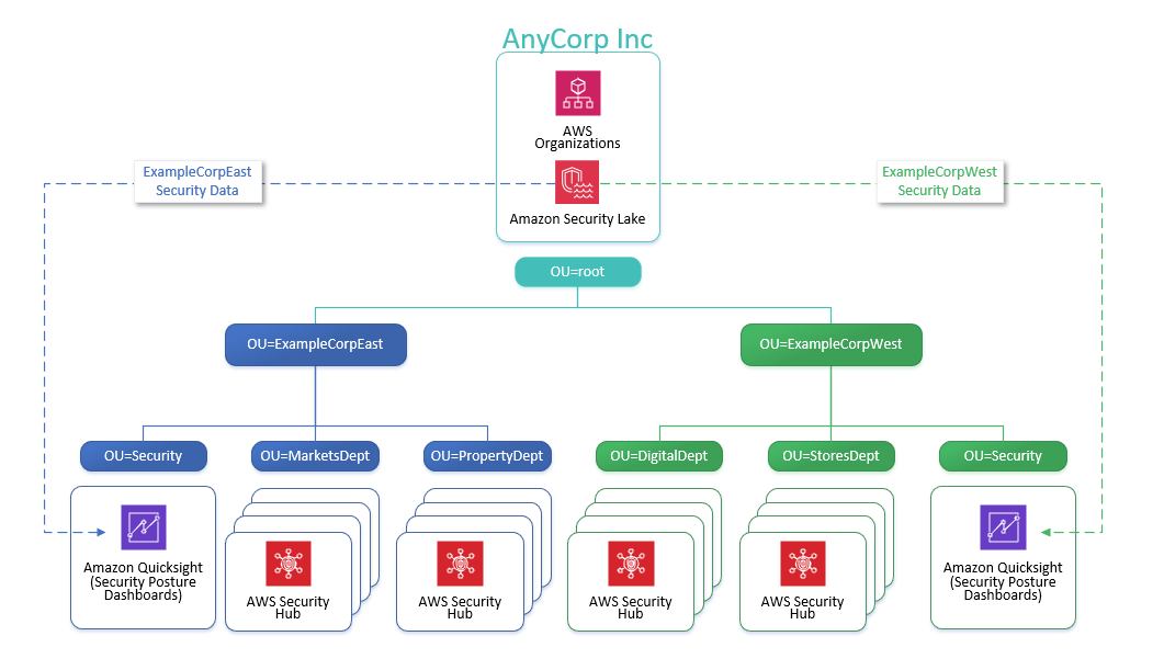
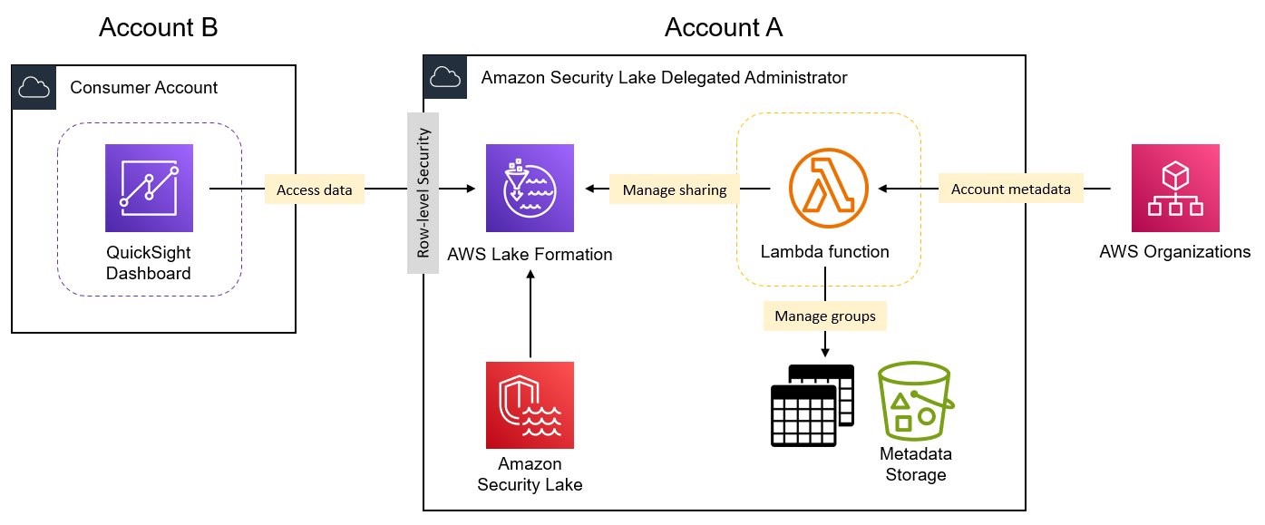
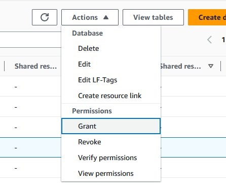
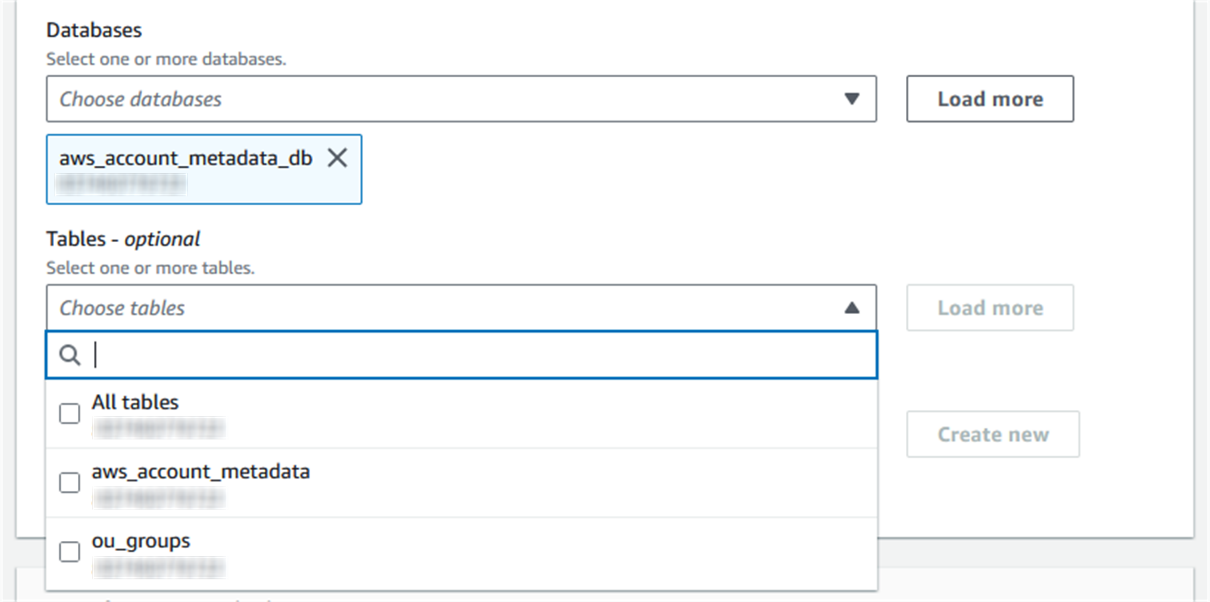
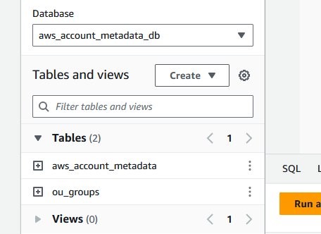
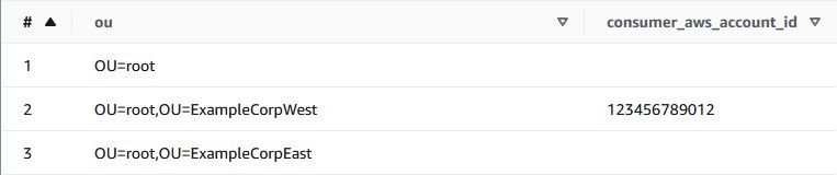

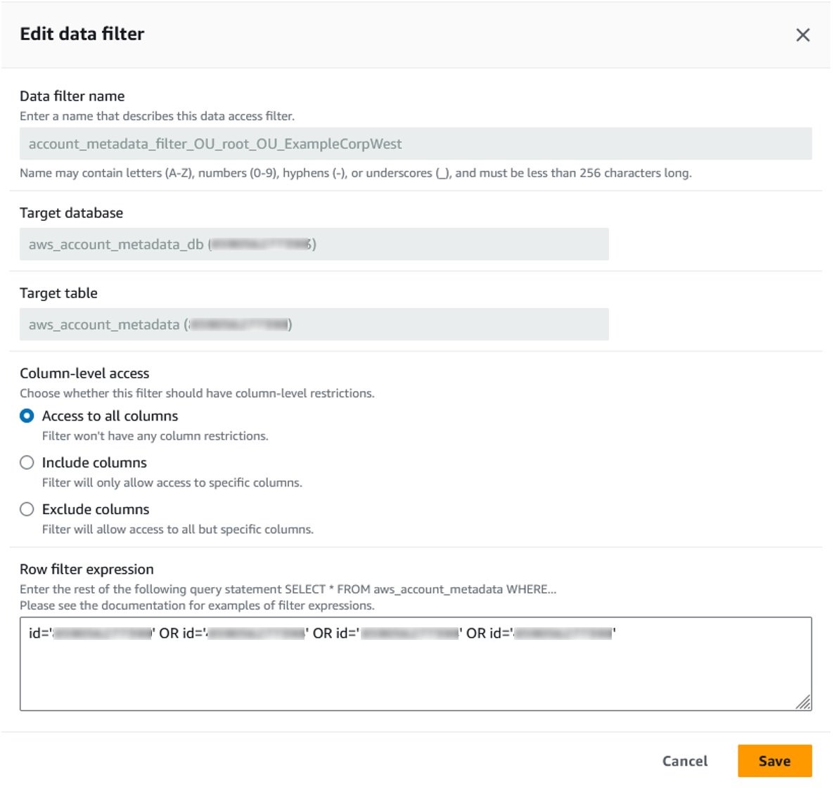
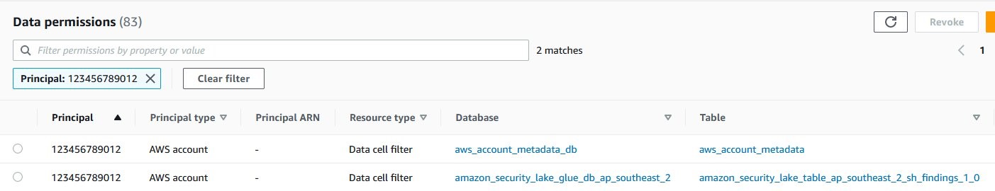
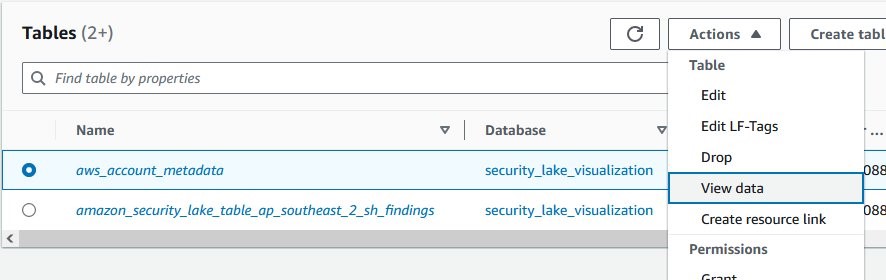
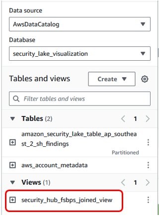
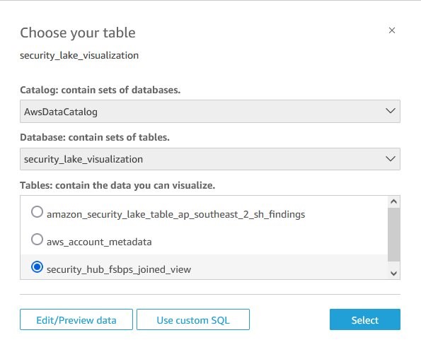
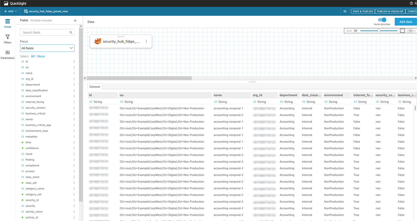
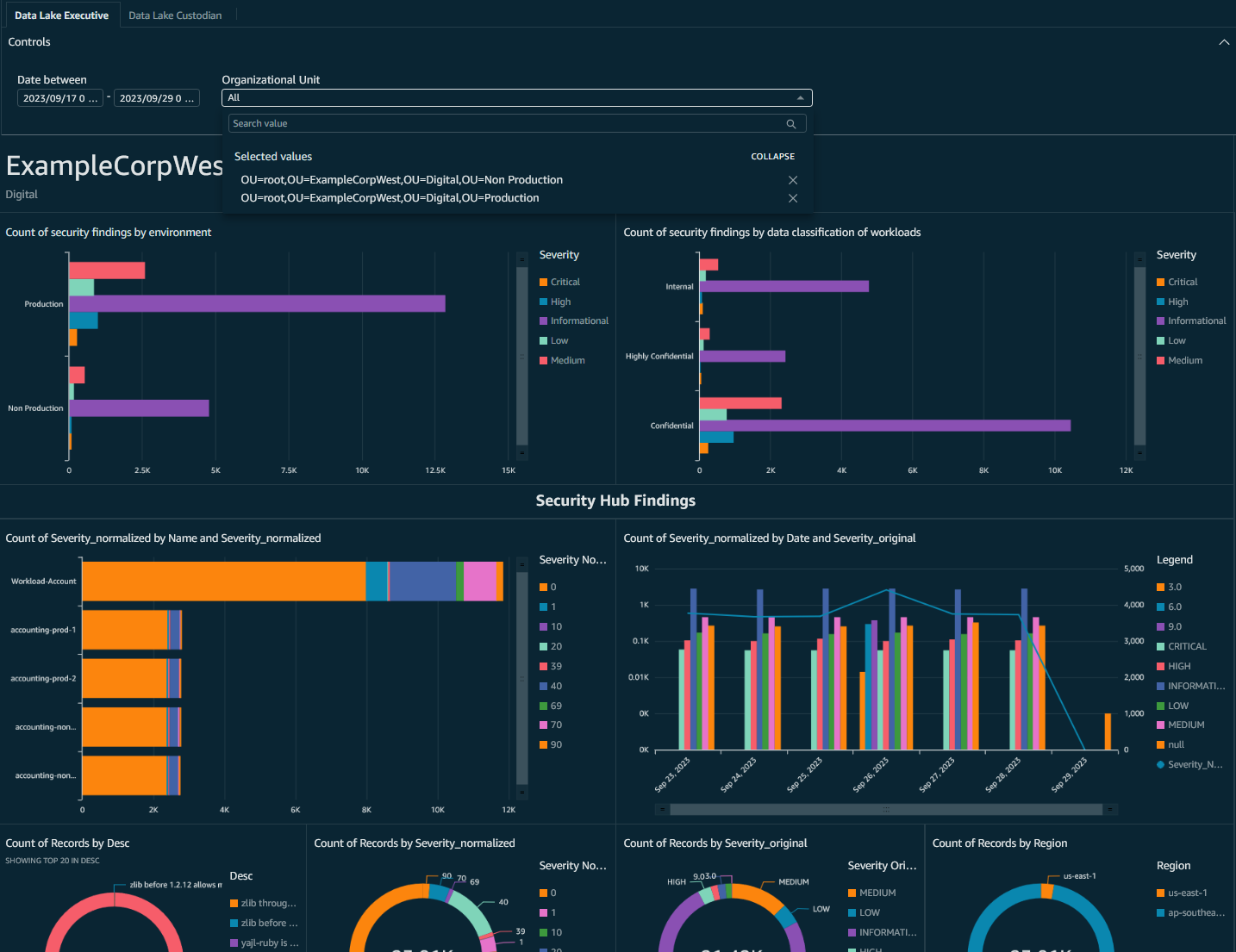


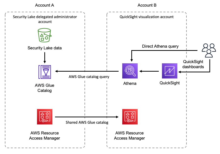
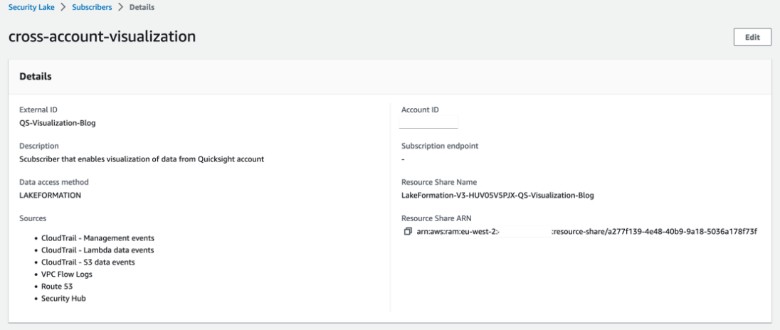


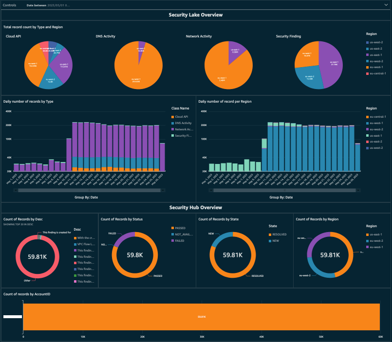
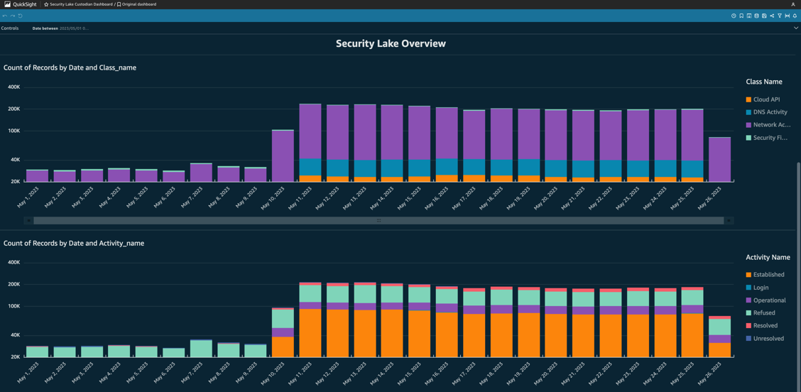
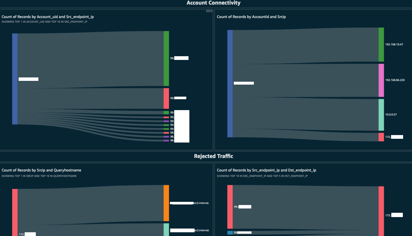


 Phil Bates is a Senior Analytics Specialist Solutions Architect at AWS. He has more than 25 years of experience implementing large-scale data warehouse solutions. He is passionate about helping customers through their cloud journey and using the power of ML within their data warehouse.
