Post Syndicated from Explosm.net original https://explosm.net/comics/accountant
New Cyanide and Happiness Comic
Post Syndicated from Explosm.net original https://explosm.net/comics/accountant
New Cyanide and Happiness Comic
Post Syndicated from Емилия Милчева original https://www.toest.bg/progresut-na-radev-trugva-s-osteritet/

Съдебната реформа е поставена на стендбай, а правителството на Румен Радев спешно търси пари – от пенсионерските ковид добавки до административните разходи. Налага се да прави и инвентаризация на скелетите в гардероба, за да оправдае обещанията за борба с корупцията. Така приключва първият месец на новото мнозинство, получило твърде много политически капитал и твърде малко финансова свобода за действие.
Каквито и наследени договори, съмнителни (и) неразплатени разходи или неизгодни решения да открива новата власт, ще трябва да намери трудното решение как да финансира собствените си политики, като се побере в лимита за дефицит от 3% от БВП.
Европейската комисия препоръча да започне процедура за прекомерен дефицит спрямо България, очаквайки превишение на разходите над приходите от 4,1% за 2026 г. и 4,3% за 2027 г. Последната дума има Съветът на ЕС. Ако предложението бъде прието, публичните финанси на България ще бъдат под надзора на Европейската комисия през следващите няколко години. Ще се наложи кабинетът да представи план с коригиращи мерки, който да договори с Европейската комисия, и до 6 месеца да започне да го изпълнява.
Правителството тепърва ще внася бюджета за 2026-та през юли, което означава, че в последните пет месеца на годината държавата ще работи с ограничен ресурс. Причината е, че Министерството на финансите (МФ) настоява да получи заявки за бюджет, който е 90% от миналогодишния, макар че през изминалите месеци структурите на бюджетна издръжка са харчили без такъв лимит.
Междувременно управляващите разкриват наследените задължения. Към май 2026 г. общият размер на неразплатените разходи от 2024, 2025 и началото на 2026 г. е бил 2,2 млрд. евро. Те включват фактурирани, но неплатени проекти на Агенция „Пътна инфраструктура“ и на общините, като тези разходи са заложени в закона за бюджета, но без да бъдат осигурени необходимите средства.
Допълнителен риск за бюджета идва от проектите по Плана за възстановяване и устойчивост (ПВУ). По тях МФ първо плаща на изпълнителите с бюджетни средства, а едва след това подава искане за възстановяване към Европейската комисия при изпълнение на съответните етапи и цели. Това означава, че всяко забавяне на реформите или на плащанията от Брюксел временно прехвърля тежестта върху българския бюджет. Така МФ се оказва принудено да финансира проекти, за които формално има европейски ресурс, но реално парите може да пристигнат много по-късно. Или да не дойдат, ако някоя от целите в Плана не е изпълнена от българските власти.
Все още не е обявено публично каква е сумата на декларираните по ПВУ за разплащане проекти.
България има и задължения по „президентския“ договор с турската компания „Боташ“, по който до май 2025 г. са платени 600 млн. лева (306,8 млн. евро), макар да е бил използван капацитет за 15 пъти по-малка сума. Ежедневно задължението на българската страна е за 1,05 млн. лв. (536 900 евро).
Темата за „Боташ“ се появява и изчезва от обществения интерес с променлива интензивност, но се зашумя отново, когато бившият енергиен министър, участвал в сключването на договора, беше назначен в Държавната консолидационна компания. Постът му стана причина лидерът на „Продължаваме промяната“ Асен Василев да обяви, че възнаграждението на Росен Христов ще е 11 160 евро, или 18 минимални работни заплати, какъвто е таванът по закон.
По-късно председателят на парламентарната група на „Прогресивна България“ Петър Витанов съобщи по bTV, че заплатата ще е 1878 евро, а Христов заплаши със съд лидера на ПП.
Проблемът за новото правителство е, че сега ще търси средства не за да реализира своите политики, а за да плаща за решения, взети от предишните управления и превърнали се в задължения на държавата.
Парадоксално, но факт. Натовареното с най-големи очаквания правителство след години на политически кризи ще трябва да ореже публични разходи, да извърши съкращения, да намали дела на сивата икономика и корупцията, ако иска да си осигури някакво финансовото благополучие и обществен престиж. Процедурата за прекомерен дефицит му развързва ръцете да предприеме непопулярни мерки, например дългоочакваната административна реформа. Абсолютното мнозинство, с което разполага, пък му осигурява необходимата подкрепа без напрежение от коалиционни партньори.
В следващите месеци кабинетът ще трябва едновременно да съкращава разходи и да убеждава избирателите, че управлява успешно. И това в навечерието на президентски избори и година преди местния вот, когато всяко евро за инвестиции в общински проекти има и политическа стойност.
Кметовете, които се канят да се присъединят към „Прогресивна България“, ще очакват финансиране на инвестиционните си проекти.
Гласувалите за Румен Радев близо 1 445 000 български граждани, които очакваха от него „да оправи държавата“, „да сложи ред“, не са очаквали остеритет.
Според Радев „тежкото наследство, което получаваме, е резултат на безхаберие, некомпетентност, волунтаризъм, популизъм и грабеж“.
Всички българи ще плащаме вересиите на олигархията и на предишните управления.
Това обяснение вероятно ще e убедително за някои избиратели. Проблемът е, че част от решенията, които днес натоварват бюджета, бяха вземани и от служебни кабинети, назначавани именно от президента Радев.
От ковид пандемията насам почти всяко управление добавяше нови постоянни разходи, без да осигурява устойчив източник за финансирането им. Временните антикризисни мерки, като интегрираните в пенсиите добавки и енергийните помощи за бизнеса, постепенно се превърнаха в трайни ангажименти. Социалните плащания и заплатите в публичния сектор растяха с темпове, които изпреварваха реалния икономически растеж.
Автоматичният механизъм за МВР и Министерството на отбраната се превърна в голям бюджетен проблем през миналата и тази година, когато започна да генерира двуцифрени годишни увеличения на възнагражденията, независимо от общото състояние на бюджета.
Тези политики на правителствата в последните пет години, които се изпълняваха и от назначените от президента Румен Радев служебни кабинети, дебалансираха бюджета. Върху тях тежат и безпринципните назначения в държавната администрация. Новата власт ще обяви огромните заплати, от порядъка на 20–25 000 евро, раздавани в държавни дружества и предприятия, които при това са на загуба.
Инвентаризацията на наследството включва и твърдения за злоупотреби при големи инфраструктурни проекти. Регионалният министър Иван Шишков вече обяви, че има подадени сигнали до прокуратурата за строителството на автомагистрала „Хемус“ и за обществени поръчки по европейски програми, поставили под риск около 127 млн. евро европейско финансиране.
Засега е ясно, че ще отпаднат автоматичните увеличения на заплатите в съдебната система и висшето образование. Дали правителството ще посмее да отреже МВР и Министерството на отбраната, които по закон трябва да получат със задна дата увеличените си отново от 1 януари 2026 г. възнаграждения?
Във Вътрешното министерство има и друг проблем – работещите пенсионери. Според отговор на министър Демерджиев на парламентарен въпрос от Мартин Димитров от „Демократична България“ към 30 април техният брой е 1098.
Засега управляващите говорят основно за съкращаване на разходи. Правителството се отказа да купува ракети за F-16 за 957 млн. долара заради липсата на средства.
Първите, които ще усетят остеритета, са пенсионерите – социалната група с най-ниски доходи. В действителност от 1 юли пенсиите им ще се увеличат с по-малко от 7,8%, защото от сегашните суми ще бъде извадена ковид добавката от 30,68 евро, а в отпуснатите нови пенсии изобщо ще липсва. Няма всички пенсионери да умрат заради 2 евро, каза Константин Проданов от „Прогресивна България“ в спор с лидера на „Продължаваме промяната“ Асен Василев.
За хората с най-ниски доходи обаче 2 евро тежат много повече от 1,09 евро по-малка субсидия за партиите, които занапред ще получават по 3 евро за всеки действителен глас.
Депутатите все още не са премахнали автоматичното увеличение на заплатите им на всеки три месеца. Тяхното основно възнаграждение се равнява на три средни в обществения сектор и в момента е 4326 евро, като към него се получават добавки за комисии и безотчетните ⅔ от тази сума за сътрудници, наем на офиси и др.
Изглежда невъзможно България да се върне към правилата от времето на валутния борд, когато държавата не си позволяваше да харчи повече, отколкото получаваше. Как ще бъдат съкратени разходите и кои социални групи ще понесат тази тежест, ще проличи още при съставянето на бюджета за тази година.
Някои икономисти вече предупреждават, че ако бюджетната консолидация не даде резултат, процедурата по свръхдефицит може да доведе не само до ограничения на разходите, но и до натиск за повишаване на данъци.
Първият месец от управлението не даде отговор дали Румен Радев ще успее да изпълни обещанията за по-малко корупция и по-ефективна държава.
Ако мнозинството обаче успее да превърне бюджетната криза в повод за реформи, може да излезе по-силно от нея. Ако се ограничи до счетоводни икономии и търсене на виновни, ще остане поредното управление, което е управлявало дефицита, вместо да се занимава с причините за него. След бюджета следва тестът със съдебната реформа.
Въпросът е дали избирателите могат да бъдат убедени, че остеритетът е промяна.
Post Syndicated from Matt Granger original https://www.youtube.com/watch?v=UMYxQx4omQo
Post Syndicated from xkcd.com original https://xkcd.com/3255/

Post Syndicated from corbet original https://lwn.net/Articles/1076478/
The Software Engineering Radio podcast has put up an
interview with graphics maintainer Dave Airlie. Much of what is in
there will not be news to LWN readers, but it is an interesting overview of
the life of a large-subsystem maintainer.
I was talking to a few of the Rust people, and I thought: these are
very young people, these are a group of people in their 20s, maybe
30s, they are a younger cohort of developers than the people I am
normally used to dealing with. I thought there was maybe a good
way we could bring these groups together. I think that having
young people coming into the kernel using Rust is valuable… So I
thought that I should be supportive of bringing Rust into the
kernel.
Post Syndicated from Hitesh Dodiya original https://aws.amazon.com/blogs/big-data/query-amazon-redshift-using-natural-language-with-kiro/
It’s Monday morning and your VP pings you: “Revenue dropped 15 percent over the weekend. What happened?” The clock starts. You open the AWS Management Console, find the right Amazon Redshift cluster, open the query editor, and start hunting. Which database has the revenue data, analytics_db or reporting_db? Is the table called orders, transactions, or sales_events? You find it, but now you need the schema. Is the amount column total_amount, revenue, or order_value? 20 minutes in, you haven’t answered the question. You’ve been navigating infrastructure.
This scenario plays out daily across data teams, and it’s why the landscape is shifting. With AI agents entering the analytics workflow, a growing number of business users can now perform complex data analysis. They no longer need to file a ticket with the data engineering team and wait days for a response. The bottleneck is no longer SQL expertise. It’s the friction between having a question and getting an answer.
The Amazon Redshift MCP server paired with Kiro removes that friction. Instead of memorizing cluster endpoints, reverse-engineering schemas, and hand-writing SQL, you describe what you need in plain text and get results. That Monday morning question becomes a single sentence: “Show me daily revenue for the past two weeks, broken down by region.” Kiro finds the cluster, discovers the schema, writes the query, and returns the answer in seconds, not minutes.
In this post, you learn how to:
You can use Kiro in two forms: Kiro integrated development environment (IDE), a full desktop development environment, and Kiro command line interface (CLI), which brings the same AI capabilities directly to your terminal. The Redshift MCP server works with both. The CLI experience is particularly well suited for the conversational analytics workflow this post describes, because you can start querying your data warehouse from a terminal session without opening an IDE.
Important: Before using this integration with production Amazon Redshift environments, read the Security tips section. This section covers critical considerations around AWS Identity and Access Management (IAM) permissions and Kiro autonomy modes.
The Model Context Protocol (MCP) is an open standard that provides AI agents with secure connections to external data sources and tools. The Amazon Redshift MCP server is an open source implementation that bridges the Kiro AI agent with your Amazon Redshift infrastructure.
With the Redshift MCP server, you can:
The server translates your natural language requests into the appropriate Amazon Redshift Data API calls and SQL queries. No manual endpoint configuration or SQL writing is required.
You might have noticed that AWS also offers the AWS MCP server (part of the Agent Toolkit for AWS), which provides broad access to AWS services, including the Redshift Data API. A common question is: if the AWS MCP server can already reach Redshift, why add a dedicated Redshift MCP server?
The two are complementary, not competing. The AWS MCP server gives Kiro general AWS capabilities (service decision guides, SDK usage guidance, troubleshooting skills, and access to AWS APIs). The Redshift MCP server adds a purpose-built analytics layer on top. It provides single-call query execution (compared to a minimum of three API calls for submit, poll, and fetch), read-only safety by default, transparent provisioned and serverless cluster handling, and dedicated metadata navigation tools. Upcoming features like query plan explanation, native identity propagation, cluster analysis, and UDF discovery will further extend this specialized layer.
You can use both together, or use the Amazon Redshift MCP server on its own. There’s no either-or requirement.
The following sections walk you through the installation and configuration process.
Before you begin, make sure that you have:
On your machine:
On AWS:
If you don’t have uv installed, run one of the following commands.
For macOS or Linux:
For Windows PowerShell:
Then install Python 3.10 or newer if needed:
Your AWS identity needs the following permissions. Attach this policy to your IAM user or role:
You also need database-level permissions: SELECT on tables you want to query, USAGE on schemas you want to explore, and connection access to the target databases.
Open (or create) your Kiro MCP configuration file and add the Amazon Redshift server.
For Kiro IDE:
~/.kiro/settings/mcp.json..kiro/settings/mcp.json.For Kiro CLI:
~/.kiro/settings/mcp.json..kiro/settings/mcp.json in your project directory.The configuration format is the same for both. Add the following:
Tip: Replace AWS_PROFILE and AWS_DEFAULT_REGION with values matching your environment. If you use AWS_REGION instead of AWS_DEFAULT_REGION, AWS_REGION takes higher precedence.
Note: Windows users: use uv instead of uvx with additional args. See the Amazon Redshift MCP server documentation for the Windows-specific configuration.
In Kiro IDE, restart Kiro (or reconnect MCP servers from the MCP Server view in the Kiro feature panel). Then open the Kiro chat and enter the following prompt:
If everything is configured correctly, Kiro discovers your clusters and lists them with details like cluster identifiers, status, node types, and endpoints.
The following scenarios show how Kiro and the Amazon Redshift MCP server work together in real-world workflows.
Tip: If you want Kiro to show the SQL that it executes alongside every result, tell it at the beginning of your session:
For every query you run against Amazon Redshift, show me the exact SQL you executed along with the results.
Kiro follows this instruction for the rest of the conversation. For a permanent setup, add this rule to a steering file (see the Tips section that follows) so you don’t need to repeat it. The following examples reflect this behavior.
Without Kiro: Log in to the AWS Management Console, navigate to Amazon Redshift, choose clusters, open the query editor, sign in to each database, and manually browse schemas.
With Kiro:
Kiro responds with a structured overview:
Found two provisioned clusters and one serverless workgroup:
Then drill deeper:
Kiro uses the MCP metadata tools to explore the cluster. No SQL is needed for discovery:
Database: analytics_db (local)
information_schema — system schemapg_catalog — system schemapublic — default schemasales — user-created schemaDatabase: dev (local)
information_schema — system schemapg_catalog — system schemapublic — default schemaThe only user-created schema is sales in the analytics_db database.
There are five base tables in analytics_db.sales:
customersorder_itemsordersproductsreturns| Column | Type | Nullable |
order_id |
INTEGER | NO |
customer_id |
INTEGER | NO |
order_date |
TIMESTAMP | NO |
total_amount |
numeric(12,2) | NO |
status |
VARCHAR(20) | YES |
Each request builds on the previous context. Kiro remembers which cluster you’re exploring and navigates the hierarchy for you.
Without Kiro: Write SQL from scratch, guess at column names, run the query, fix syntax errors, iterate.
With Kiro:
Kiro does the following:
The response includes the query and results:
Query executed:
| customer_id | customer_name | total_orders | total_spent |
| 4821 | Acme Corp | 347 | $1,284,500.00 |
| 1190 | Globex Inc | 289 | $1,102,340.00 |
| 7734 | Initech LLC | 256 | $987,210.00 |
| … | … | … | … |
You didn’t need to remember table names, column names, or join conditions. Kiro figured it out by exploring the metadata first. You can see exactly what it ran, copy the SQL, and reuse it.
Without Kiro: Open two SQL clients, sign in to different clusters, run similar queries, manually compare results in a spreadsheet.
With Kiro:
Kiro queries both environments, aligns the results, and provides a comparison, showing every query it runs along the way.
Query executed on analytics-cluster:
Query executed on etl-workgroup:
Sales data comparison: Analytics vs ETL.
| Metric | Analytics Cluster | ETL Workgroup | Status |
| Total Records | 172,456 | 172,456 | Match |
| Total Revenue | $110,765,431 | $110,765,431 | Match |
| Q4 Transactions | 38,061 | 38,061 | Match |
Because both queries are visible, you can verify that Kiro compared the same metrics on both sides, with no hidden assumptions.
Without Kiro: Manually document table structures in a wiki or spreadsheet. Documentation frequently falls out of date.
With Kiro:
Kiro explores every table using the discovery tools and produces structured documentation.
Table: sales.customers
| Column | Type | Nullable | Description |
customer_id |
INTEGER | NO | Primary key |
customer_name |
VARCHAR(255) | NO | |
email |
VARCHAR(255) | YES | |
created_at |
TIMESTAMP | NO |
Table: sales.orders
| Column | Type | Nullable | Description |
order_id |
INTEGER | NO | Primary key |
customer_id |
INTEGER | NO | FK to customers |
order_date |
TIMESTAMP | NO | |
total_amount |
numeric(12,2) | NO | |
status |
VARCHAR(20) | YES |
(continues for all tables in the schema…)
You can paste this directly into your team wiki or README, and anyone can rerun the same discovery flow to refresh the docs later.
Query executed:
Out of 172,456 rows: 0 NULL customer_ids, 3 NULL total_amounts.
Query executed:
Found two duplicate order_ids: order 88412 (two occurrences), order 91003 (two occurrences).
Query executed:
Date range: 2024-01-01 to 2025-04-20. Found three missing dates: 2024-03-15, 2024-07-04, 2024-12-25 (likely holidays).
Every query is right there in the response. You can copy them into your own SQL client, modify them, or save them as reusable scripts.
.kiro/steering/redshift.md file in your project with details about your cluster naming conventions, important schemas, and common query patterns. This gives Kiro persistent context about your environment.Example steering file:
That last Query Transparency rule is a small addition with a big impact. By default, Kiro might summarize results without showing the underlying SQL. Adding this steering instruction makes every query visible, which helps maintain consistent behavior across your data team and supports auditing, learning, and trust.
When configured with least privilege IAM policies and Supervised mode, the Redshift MCP server provides multiple layers of protection. Under the AWS shared responsibility model, you are responsible for configuring access controls appropriately.
Important caveat: The read-only enforcement only applies to queries routed through the MCP server’s execute_query tool. Kiro also has shell access. If your IAM credentials have write permissions, direct CLI calls (aws redshift-data execute-statement) bypass this guardrail entirely.
Takeaway: Use least privilege IAM policies (scoped to read and describe operations only) as your primary defense. Avoid broad policies like AdministratorAccess or AmazonRedshiftFullAccess. When IAM is properly scoped, even a direct CLI call cannot perform writes.
Kiro is a powerful assistant, but it’s not infallible. Like any AI tool, it can misinterpret your intent, generate incorrect SQL, or present results that look plausible but are wrong. Examples include a misplaced join, a wrong filter, or an aggregation that silently excludes rows. This is especially important when working with production data where decisions have real business impact.
Treat Kiro’s output as a strong starting point, not a final answer. Review the SQL it generates before acting on the results. Use the Query Transparency steering rule (described in the Tips section) so you can see the exact query behind every result. When findings inform business decisions, validate them independently by running the query yourself, cross-checking with a colleague, or comparing against a known baseline.
| Layer | What it protects against |
| MCP server read-only mode | Accidental writes through the MCP execute_query tool |
| Least privilege IAM policy | Write operations via any path, including direct CLI calls |
| Kiro Supervised mode | Unreviewed autonomous actions by the agent |
Defense in depth: use these layers together for production environments.
| Before | Now you can |
| Switch between the console, SQL clients, and documentation | Use one interface for discovery, querying, and analysis |
| Memorize cluster endpoints, database names, and schemas | Ask in plain text and let Kiro discover the structure |
| Write SQL from scratch for every query | Describe what you want and get results |
| Manually compare data across clusters | Run single-sentence cross-cluster analysis |
| Schema documentation is frequently stale | Generate fresh docs on demand |
| Onboarding new analysts takes days | New team members can explore immediately |
Every minute you spend hunting for a table name or debugging a SQL syntax error is a minute that you’re not spending on actual analysis. You can reduce that overhead by letting Kiro handle the mechanical parts (discovery, navigation, and query construction) so you can focus on the questions that matter to your business.
If you created Amazon Redshift resources specifically for this walkthrough, or if you no longer need the MCP server integration, follow these steps. They help you avoid ongoing charges and remove the configuration.
In this post, you learned how to set up Kiro with the Amazon Redshift MCP server to query your data warehouse using natural language. You explored cluster discovery, schema browsing, analytical queries, cross-cluster comparisons, and data quality checks, all without writing SQL from scratch or switching between tools.
To go further:
As you get comfortable with the basics, try combining steering files with agent hooks to automate recurring workflows like daily data quality checks or weekly schema documentation refreshes.
Post Syndicated from Howie Li original https://aws.amazon.com/blogs/security/amazon-cognito-unlocks-advanced-capabilities-with-next-generation-infrastructure/
Amazon Cognito recently introduced high-throughput performance for demanding workloads, customer-managed keys for full control over data encryption at rest, and multi- Region replication for business continuity improvement. These capabilities were made possible through a next-generation storage infrastructure designed for extensibility and scale. To deliver this, we migrated hundreds of millions of user profiles, and you probably didn’t even notice. In this post, we walk through what’s new, the architecture behind it, and how we got here with a zero-downtime migration that kept your applications running.
The migration to the new infrastructure wasn’t just about maintaining existing functionality—it created the foundation for delivering capabilities that solve customer challenges while positioning Amazon Cognito for continuous improvements.
High-throughput performance: The new architecture supports the higher request volumes and scale requirements of modern applications while maintaining the low latency performance that your applications depend on—able to support tens of millions of users per user pool and thousands of transactions per second (TPS).
Customer-managed keys: Customers can now use their own encryption keys stored in AWS Key Management Service (AWS KMS) for encrypting data at rest. This provides enhanced security control and capabilities, giving customers full ownership over their encryption key lifecycle.
Multi-Region replication: Customers can now synchronize their entire user pool data, including user passwords, attributes, and configurations to another user pool in another Region of their choice. This means that customers can implement business continuity strategies and maintain authentication availability in case of a Regional failover, helping their applications remain accessible to users even during unexpected disruptions.
The new architecture uses a purpose-built storage layer designed for extensibility and scale of identity operations. We anchored the new architecture around a set of design tenets:
These tenets shaped every architectural decision. The architecture separates into independently deployable domains. Previously, while using Amazon Cloud Directory, the service architecture relied on a single data store to persist all customer information. This provided straightforward data traversal mechanisms but required multi-service coordination to adjust database schema when new features were required. The new architecture uses different datasets, allowing them to evolve independently for faster feature iterations.
Migrating users requires extreme precautions and a strategy designed to maintain zero downtime and ensure data integrity at every step. Our approach prioritizes both immediate stability and long-term flexibility through the following measures:
This modernization taught us valuable principles that apply to any large-scale infrastructure project, therefore we choose to share these learnings to help you perform similar migrations.
In this post, we shared the high-level approach and learnings from the Amazon Cognito infrastructure modernization that create a foundation for modern identity management capabilities. The new Cognito infrastructure is live, delivering capabilities such as customer-managed keys and multi-Region replication. As the migration continues, all Cognito customers will gain access to these capabilities on the same service they rely on today, with no action required.
Ready to modernize your authentication infrastructure? Visit Amazon Cognito to learn more.
If you have feedback about this post, submit comments in the Comments section below.
Post Syndicated from The Atlantic original https://www.youtube.com/shorts/hwb4g7KGYp4
Post Syndicated from Ken Kitts original https://aws.amazon.com/blogs/security/gain-visibility-into-ddos-attacks-with-flow-logs-in-aws-shield-advanced/
Reconstructing distributed denial of service (DDoS) attack traffic used to mean combining data from multiple sources after the fact. AWS Shield Advanced attack flow logs change that—they capture traffic metadata during attacks so you can pinpoint sources, verify mitigations, and feed your existing analysis pipelines.
Shield publishes logs to Amazon Simple Storage Service (Amazon S3), Amazon CloudWatch Logs, or Amazon Data Firehose using the same CloudWatch Logs delivery infrastructure as other AWS flow logs, so they fit directly into the monitoring and analysis tools you already use.
In this post, you will learn how Shield Advanced attack flow logs capture metadata during DDoS events, what each field in a flow log entry means, and how to enable and configure flow logging for your protected resources.
A DDoS attack floods an application with traffic, making it unavailable to users. Infrastructure-layer attacks saturate bandwidth and exhaust connection tables—you see packet loss and timeouts.
Shield Advanced is a managed DDoS protection service that detects and mitigates attacks for Amazon CloudFront distributions, Elastic Load Balancing load balancers, Amazon Route 53 hosted zones, AWS Global Accelerator standard accelerators, and Elastic IP (EIP) addresses. See the AWS Shield Advanced documentation for full coverage details. Initially, Shield Advanced will provide infrastructure-layer attack flow logs for EIP protections, with support for additional resource types to follow.
Flow logs help you understand attacks in several ways:
srccountry and location fields show where traffic originated and which AWS edge location it entered.Logs go to Amazon S3, CloudWatch Logs, or Data Firehose. You can then query them with Amazon Athena (a serverless query service for analyzing data in Amazon S3), route them to third-party Security Information and Event Management (SIEM) platforms or build CloudWatch Logs Insights queries (an interactive log analysis feature) without deploying new infrastructure.
Log records capture source and destination IP addresses and ports, protocol, packet and byte counts, the action Shield Advanced took, and TCP flags. They also include the AWS ingress location where traffic entered and a two-letter country code for the traffic source when available. Logs are written at 5-minute intervals and are available during an active attack and after it concludes.
The maximum file size is 75 MB. If a file reaches that limit within the 5-minute window, the file will be closed, published, and a new file will start. Flow logs support JSON, plain text, W3C, and Parquet output formats and contain the following fields:
| Field | Description |
| protection_arn | Amazon Resource Name (ARN) of the Shield protection |
| event_timestamp | Timestamp of log generation |
| version | Flow log version number |
| srcaddr | Source IP address |
| dstaddr | Destination IP address |
| srcport | Source port |
| dstport | Destination port |
| protocol | IP protocol number |
| packets | Packet count within the aggregation window |
| bytes | Byte count within the aggregation window |
| starttime | Aggregation window start time |
| endtime | Aggregation window end time |
| action | Action taken by Shield |
| location | AWS ingress location |
| sampling_rate | Sampling rate used during packet processing |
| tcp_flags | TCP flags from the packet |
| srccountry | Two-letter country code for the traffic source |
The following steps walk you through creating the CloudWatch Logs delivery resources that connect a Shield Advanced protection to your preferred log destination.
Before configuring flow logs, make sure you have:
logs:PutDeliverySource, logs:PutDeliveryDestination, logs:CreateDelivery)Flow logs incur standard CloudWatch Logs vended log charges, and the destination resources (S3 bucket storage, CloudWatch Logs log group storage, or Firehose data processing) incur separate charges. Review the Vended Logs entry on the CloudWatch pricing page and the pricing for your chosen destination service before enabling flow logs on high-traffic resources.
Log delivery requires three objects:
This three-object model lets you reuse destinations across multiple sources and manage delivery pipelines independently. For example, you can send logs from multiple Shield protections to the same S3 bucket by creating multiple DeliverySource objects that reference the same DeliveryDestination.
Because Shield Advanced attack flow logs use the CloudWatch Logs delivery infrastructure, you can aggregate them across accounts and Regions just like other vended logs. Deliver directly to a centralized S3 bucket with a cross-account policy, replicate CloudWatch Logs log groups using cross-account cross-Region centralization rules, or stream to a shared Firehose stream using cross-account subscriptions. Explore these options to build a unified view of DDoS attack traffic across your multi-account, multi-Region footprint.
Choose a destination:
The destination resource needs a policy that grants the CloudWatch Logs delivery service write permissions. The policy varies by destination type. For more information, see Logs sent to Amazon S3, Logs sent to CloudWatch Logs, or Logs sent to Firehose.
For Amazon S3 destinations, you have two options:
s3:GetBucketPolicy and s3:PutBucketPolicy permissions, AWS automatically creates the required policy when you create the delivery in step 6. You can skip to step 3.Shield Advanced is a global service and uses the us-east-1 AWS Region for management. Run the following command to list your Shield Advanced protections.
In the output, copy the ProtectionArn value for the protection you want to log.
Run the following command to create the delivery source, replace <protection-arn> with the ProtectionArn value from step 3.
The --resource-arn is the ARN of your Shield Advanced protection—not the protected resource itself. Shield Advanced creates a separate protection object that wraps your resource, and flow logs are generated by that protection layer rather than the underlying resource.
Run the following command to create the delivery destination, replace <resource-arn> with the ARN of the destination resource you created in step 1.
The --delivery-destination-configuration parameter takes a JSON object with a destinationResourceArn key whose value is the ARN of your S3 bucket, log group, or Firehose stream.
In the output, copy the value of the top-level ARN field—this is the delivery destination ARN (different from the bucket ARN). You will use this in step 6.
Run the following command to connect the delivery source to the delivery destination, replace <delivery-destination-arn> with the delivery destination ARN from step 5.
Run the following command to confirm the delivery is active.
After delivery is active, Shield Advanced publishes flow log records to your destination during DDoS events.
To avoid ongoing charges, delete the resources you created.
For an S3 bucket:
For a CloudWatch Logs log group:
For a Firehose stream:
Shield Advanced attack flow logs provide the visibility you need to understand and respond to DDoS attacks effectively. By integrating with your existing observability infrastructure, they deliver actionable insights without requiring new tooling or complex setup. Enable flow logs on your Shield Advanced protections today to gain immediate visibility into attack patterns and strengthen your DDoS defense posture.
For the full reference about flow log configuration, see the AWS Shield Advanced documentation.
If you have feedback about this post, submit comments in the Comments section below.
Post Syndicated from Bruno Giorgini original https://aws.amazon.com/blogs/messaging-and-targeting/getting-started-with-amazon-ses-agent-skills-for-ai-assisted-email-development/
Building email infrastructure with Amazon Simple Email Service (SES) involves navigating identity verification, authentication protocols, configuration sets, bounce handling, and deliverability monitoring. Developers often spend time reading documentation and iterating on API calls before getting their first email sent correctly. AI coding agents can accelerate this process, but without domain-specific context, they frequently generate code using the legacy V1 API, skip authentication setup, or miss production requirements like tenant isolation.
Today, we are releasing Amazon SES Agent Skills, an open source set of agent skills that give AI coding agents the context they need to build email integrations correctly from the start. The skills work with Kiro, Claude Code, and any agent that supports the open Agent Skills format.
Agent skills are structured context packages that teach AI agents how to use a specific service correctly. Rather than relying on general training data (which may be outdated or incomplete), a skill provides the agent with validated patterns, common mistake avoidance, and step-by-step workflows for a specific domain.
When you install the Amazon SES agent skills, your AI agent gains access to:
Amazon SES has two distinct capabilities that use different API clients:
| Skill | Use case | SDK client |
|---|---|---|
aws-ses |
Sending email (transactional, marketing, notifications) |
sesv2 |
aws-mail-manager |
Receiving and processing inbound email (routing, filtering, archiving, SMTP relay) |
mailmanager |
These are different APIs with different clients. A common mistake agents make without this context is mixing them up or using the legacy ses client for sending.
Install both skills:
npx skills add amazon-ses/skills
Or install a specific skill:
npx skills add amazon-ses/skills --skill aws-ses
npx skills add amazon-ses/skills --skill aws-mail-manager
Once installed, the skill activates automatically when you ask your agent about email-related tasks.
After installing the aws-ses skill, ask your agent: “Help me send my first email with Amazon SES.”
Without the skill, an agent might generate code using the deprecated V1 API, skip identity verification, or omit a configuration set. With the skill, the agent follows the correct workflow:
Here is an example of what the agent produces for a Python quickstart:
import boto3
from botocore.exceptions import ClientError

client = boto3.client('sesv2', region_name='us-east-1')

try:
    response = client.send_email(
        FromEmailAddress='[email protected]',
        Destination={'ToAddresses': ['[email protected]']},
        Content={
            'Simple': {
                'Subject': {'Data': 'Hello from Amazon SES'},
                'Body': {'Text': {'Data': 'This email was sent using Amazon SES V2 API.'}}
            }
        },
        ConfigurationSetName='my-config-set',
        TenantName='my-tenant'
    )
    print(f"Message sent: {response['MessageId']}")
except ClientError as e:
    print(f"Send failed: {e.response['Error']['Code']} - {e.response['Error']['Message']}")
The agent knows to use sesv2 (not ses), includes a configuration set for observability, uses a tenant for isolation, and sends to a simulator address for safe testing.
For inbound email processing, the aws-mail-manager skill teaches the agent the core pipeline architecture:
Internet → Ingress Point → Traffic Policy → Rule Set → Action
The skill ensures the agent creates resources in the correct dependency order (traffic policy and rule set before ingress point), uses the correct condition syntax (union types with exactly one key per object), and waits for the ingress point to reach ACTIVE status before recommending DNS changes.
Each skill contains:
The agent loads only the context relevant to your current task. Ask about sending email and it loads the sending guides. Ask about archiving inbound email and it loads the archive reference.
To use the skills, you need:
boto3), Node.js (@aws-sdk/client-sesv2), or Java (software.amazon.awssdk:sesv2)The Amazon SES Agent Skills are available now on GitHub:
Install the skills, ask your agent to help you send your first email, and see how structured context changes the development experience. If you find issues or want to contribute, open an issue or pull request on the repository.
Post Syndicated from corbet original https://lwn.net/Articles/1075838/
The splice()
and vmsplice()
system calls are meant to improve performance for certain data-movement
tasks by minimizing (or avoiding altogether) system calls and the copying
of data. They also have a long history of security problems. The recent
flood of LLM-discovered vulnerabilities has drawn attention, once again, to
splice() and vmsplice(); as a result, they may end up
being removed altogether.
Post Syndicated from LastWeekTonight original https://www.youtube.com/watch?v=UMG5_6ybpV0
Post Syndicated from LastWeekTonight original https://www.youtube.com/shorts/quoewSXtGq4
Post Syndicated from Abrom Douglas original https://aws.amazon.com/blogs/security/customize-federated-sign-in-with-new-amazon-cognito-lambda-trigger/
You can use Amazon Cognito user pools to add sign-up and sign-in functionality to your web and mobile applications. You can authenticate users directly with Amazon Cognito managed accounts using passwords, passwordless flows, or custom authentication flows, or let users federate in through external identity providers (IdP) using SAML, OpenID Connect, or social providers such as Google, Facebook, Sign in with Apple, or Login with Amazon. For consumers, identity federation means fewer passwords to remember and a smoother sign-in experience. For business-to-business (B2B) software as a service (SaaS) providers, it means your tenants’ organizations keep control of their own identities rather than managing credentials on their behalf. But federation can also introduce challenges for enterprises and application developers. What happens when your enterprise customer’s SAML provider sends hundreds of group memberships that exceed attribute size limits? Or when your ecommerce customer forgets they already have an account and tries to sign in with a different social provider, creating duplicate records?
In this blog post, I introduce the inbound federation Lambda trigger for Amazon Cognito, a new feature that gives you programmatic control over federated authentication flows. This AWS Lambda trigger intercepts the federated authentication response immediately after your external identity provider responds to Cognito, so you can transform, filter, and enrich user attributes before the user profile is created and user attributes are mapped in your user pool.
The inbound federation Lambda trigger is invoked after your Amazon Cognito user pool has received and verified the response from the external IdP. The request payload for the federated IdP response is then sent from Cognito to your Lambda function and you will receive the following information:
userPoolId and clientId)providerName)providerType (SAML, OIDC, Login with Amazon, and so on)The specific format of this attribute data depends on the provider type, view the Inbound federation Lambda trigger parameters section in the docs to learn more. If the external IdP is a SAML provider, you will receive a JSON key-pair listing of the user’s attributes from the IdP assertion. If the external IdP is an OIDC provider (or social provider), you will receive the access token and attribute data from the /userinfo endpoint, along with an ID token if one was provided. See Figure 1 for a detailed flow of a federated sign-in with an Amazon Cognito user pool configured to use the inbound federation Lambda trigger.
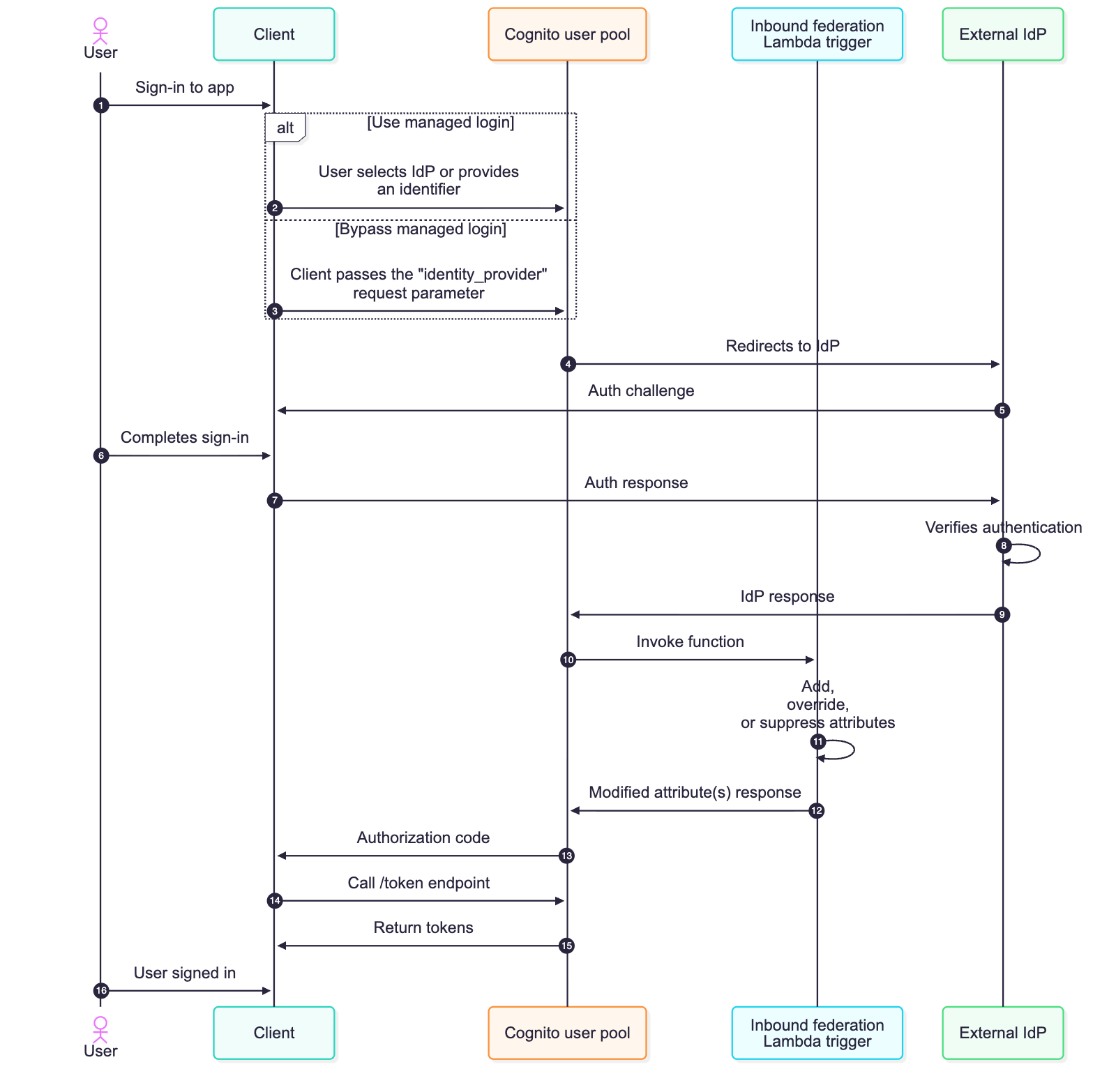
Figure 1: Sequence flow of a federated login configured with the inbound federation Lambda trigger
/token endpoint with the authorization code.Federation introduces complexity that varies depending on your use case. For B2B and SaaS applications, you’re often not in control of your customers’ IdPs, including what attributes they send or how they format them. As an example, an enterprise customer will configure their SAML response to include every group a user belongs to. This could be hundreds of groups or long group identifiers, and if the group membership of the user is mapped to an Amazon Cognito attribute, this can lead to a scenario where the Cognito attribute size limit is exceeded, causing federated sign-ins to fail.
Challenges for business-to-customer (B2C) applications can differ from B2B use cases. For B2C applications, organizations shouldn’t be required to think about identity providers. The ability to sign-up and sign-in should be seamless for consumer-facing applications. Customers visiting a consumer-facing application might create an account with email and password, forget they created created it, and then later try signing in with Facebook (or other social provider). Without proper account linking in Amazon Cognito, you then have multiple user records for the same user, which could lead to fragmented purchase history and a frustrating customer experience.
Both B2B and B2C use cases might need to look up external data just prior to completing the sign-in process, such as additional roles and access for B2B users or looking up active orders for B2C users. Another example could be the need to normalize data just prior to storing it in the user profile within the Amazon Cognito user pool or even discarding personally identifiable information (PII) prior to storing it in your Cognito user pool.
With the inbound federation Lambda trigger, you can handle these B2B and B2C use cases programmatically, and do so without requiring modification of your applications or coordinating IdP-specific changes with external IdPs. In this section, I dive deeper into two common use cases: oversized group attributes, common with B2B customers, and automated account linking, common with B2C customers.
If you have B2B and SaaS use cases, it’s a common practice to use group membership from the IdP to determine the level of access you have within the SaaS service. This is a great way to still provide some access control back to the enterprise customers themselves. The groups can be used to represent the roles a user will have or for some form of coarse-grained authorization. However, your customers might inadvertently send a large number of groups a user is a member of, thus leading to an oversized attribute payload.
Another common scenario is where the syntax and format of group name a user belongs to can arrive in various formats across different IdPs; such as a canonical name (for example, example.com/groups/myApp-readOnly), a distinguished name (common with LDAP based systems and such as cn=myApp-readOnly,OU=groups,DC=example,DC=com), or a plain text string (such as myApp-readOnly). Instead of having downstream authorization logic to accommodate different variations of a group name, you can now normalize how groups are represented prior to storing the user’s attribute data using the inbound federation Lambda trigger.
To expand this, imagine your enterprise customer uses a SAML IdP, such as Active Directory Federation Services (AD FS), in front of Active Directory (AD). When their users authenticate, AD FS sends a groups attribute containing every AD group the user belongs to. For users in large organizations, this can be hundreds of groups, and the attribute is mapped to an Amazon Cognito attribute, this could result in a string that exceeds 2,048-character limit per attribute of Cognito. Authentication would fail in this scenario, ultimately leading to support tickets because enterprise customers would be unable to sign in. Even if certain users didn’t exceed this limit, because of a smaller number of group memberships, this would result in the collection and storing of unnecessary data in your Cognito user pool.
Previously, you would need to work with your customer’s IT department to modify their SAML configuration to filter groups at the source—a process that could take weeks and require multiple approval cycles because it involves a change to the federation configuration. Especially for SaaS customers, this isn’t a scalable approach because you could integrate with hundreds of external IdPs. With the inbound federation Lambda trigger, you can solve this by filtering the groups to only those relevant to your application and normalizing the nomenclature of these groups. The following Lambda function filters the groups attribute to include only groups relevant to your application and normalizes the names of groups.
This approach reduces a large group list to only what is applicable to your application. Authentication succeeds, and you maintain control over your user pool’s data without depending on external configuration changes.
The second use case addresses a challenge that’s particularly common in B2C facing ecommerce or any consumer-facing applications; although it can also be applicable to B2B scenarios. Imagine you’re running an online retail store. A customer creates an account with their email and password to make a purchase. A few months later, they return to your site but forgot they already created an account and they see the Login with Amazon button and decide to sign in this way. Without account linking, Amazon Cognito creates a new federated user because these are technically distinct accounts, and now this customer has two separate accounts with different purchase histories and saved preferences.
This fragmentation creates a poor customer experience and complicates your business operations. You can’t see the customer’s complete purchase history, loyalty points are split across accounts, and your analytics show two distinct customers instead of one.
The inbound federation Lambda trigger can be used to solve this by automatically linking federated identities to existing local accounts based on email address. While account linking can also be implemented in a pre-sign-up Lambda trigger, the inbound federation trigger runs on every federated sign-in, not just the first, giving you access to the latest IdP attributes and the ability to apply linking logic continuously rather than only at initial account creation. If no local Amazon Cognito account exists, you can create one and then link the social provider account to it. The local account can serve as the primary identity, ensuring consistent JSON Web Tokens (JWTs) regardless of how the user signs in. The following is an example of an inbound federation Lambda trigger that can help address this use case.
Every federated sign-in will invoke the inbound federation Lambda trigger, and the logic is straightforward. When a user authenticates with an external identity provider, the trigger extracts their email from the federated response and searches the user pool for a local Cognito account with that same email. If one exists—such as if the user originally signed up with email and password—the Lambda function links the federated identity to that existing local account. If no local account exists, the trigger creates one on the fly as a passwordless account (confirmed, suppressing any emails, and ready for passwordless email one-time passcode (OTP) sign-in), then links the federated identity to it. In both cases, the local account is set as the primary profile. This means the user’s JWTs always carry the same sub-claim regardless of how they sign in—directly, or through Google, Facebook, or SAML—your application sees one consistent identity. The preceding Lambda trigger is also smart enough to check whether a linked account already exists before making the call, so returning users who’ve already been linked don’t generate unnecessary API calls. And because the local account supports passwordless authentication, a user who first arrived through federation can later sign in directly with an emailed OTP—or even add a password later through your applications account settings. The local account is always the anchor.
As you implement these patterns, keep a few best practices in mind. Your Lambda function must be completed within 5 seconds, so optimize for speed to help ensure the federated sign-in process is able to successfully complete. If you’re making external calls within the inbound federation Lambda function, like Amazon DynamoDB queries or API requests, implement caching where possible. Handle errors gracefully—if your Lambda function throws an exception or an error, authentication could fail for the user. Consider logging the error and returning the original event back to Amazon Cognito rather than failing authentication for a legitimate user attempting to sign in. Here are some additional best practices for working with Lambda functions.
For the account linking use case, automatic linking relies on matching the email from the federated identity to a local account. However, there are scenarios where this match won’t exist. For example, Apple’s Hide My Email feature generates a unique alias for each app, so the federated email won’t match any existing local account. This is an effective privacy feature but it also blocks the ability to automatically link accounts. In cases like these, your application will need to implement a user-initiated account linking flow, such as prompting the user to verify ownership of both email addresses before calling the AdminLinkProviderForUser API to complete the link.
Monitor your Lambda function performance using Amazon CloudWatch metrics. Set up alarms for errors, timeouts, and throttling so you can respond quickly if issues arise. I also recommend capturing sample event payloads from a CloudWatch log group during your initial development and deployment—these will be valuable for local testing and debugging which can lead to quicker resolution if issues arise in your production environment. This is especially important as different IdPs (namely SAML and OIDC providers) may respond with varying attribute and value syntaxes. Consider implementing CloudWatch alarms to alert your security and operational teams if authentication failures spike, which could indicate an attempted attack, misconfiguration, or provide insight into further optimization of your inbound federation Lambda trigger.
In this post, you learned about the new inbound federation Lambda trigger for Amazon Cognito and how it can solve various use cases. You walked through two common federation challenges and reviewed some sample code to help resolve those challenges. For B2B and SaaS applications, the inbound federation Lambda trigger gives you control when dealing with oversized attributes from external identity providers (such as group membership) without requiring coordination with enterprise IT teams. For B2C and consumer-facing applications, it enables seamless account linking across multiple authentication methods, creating a unified customer experience.
The new Lambda trigger works with SAML, OIDC, and supported social providers, and is available now in AWS Regions where Amazon Cognito is available. To learn more about the new Lambda trigger and others, see the Amazon Cognito Developer Guide.
What federation challenges are you facing in your applications? I’d love to hear about your use cases in the comments below and over at AWS re:Post.
Post Syndicated from Steve Phillips original https://aws.amazon.com/blogs/big-data/build-governance-dashboards-for-amazon-sagemaker-catalog-with-amazon-quick/
Maintaining visibility into your data catalog’s health requires more than ad-hoc queries. Data stewards and compliance teams need automated dashboards that surface governance metrics and alert them when issues arise. These issues include undocumented assets, missing ownership, and stale metadata.
In a previous post, we showed you how to query Amazon SageMaker Catalog metadata using SQL by using the metadata export feature. This post builds on that foundation by demonstrating how to create governance dashboards with Amazon Quick.
Amazon Quick is an agentic AI-powered digital workspace that provides integrated analytics, automation, and research capabilities. With Amazon Quick Sight, a component of Amazon Quick, you can create interactive dashboards and visualizations with automatic chart suggestions and machine learning (ML) insights.
We walk through how to connect Amazon Quick Sight to your Amazon SageMaker Catalog metadata and build governance dashboards using natural language prompts.
This solution extends the metadata export architecture by adding a visualization layer:
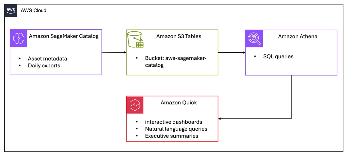
Figure 1 – Amazon SageMaker Catalog governance dashboard architecture
Before you begin, complete the following steps from Analyzing your data catalog: Query SageMaker Catalog metadata with SQL. You must also have the following:
asset_metadata.asset table contains dataAdditionally, you need:
To visualize catalog health metrics, connect Amazon Quick Sight to your Athena metadata tables.
The Amazon Quick Sight service role (default name: aws-quicksight-service-role-v0) needs permissions to access Amazon S3 Tables and AWS Glue catalog:
Add this as an inline policy to the Amazon Quick Sight service role in the IAM console.
Both the Amazon Quick Sight service role and your Amazon Quick Sight admin user need AWS Lake Formation permissions on the S3 Tables catalog. First, find your Amazon Quick Sight admin user ARN by running this AWS Command Line Interface (AWS CLI) command:
Amazon Quick Sight users are managed in the Amazon Quick Sight home AWS Region (us-east-1).To grant permissions, use the Lake Formation console.
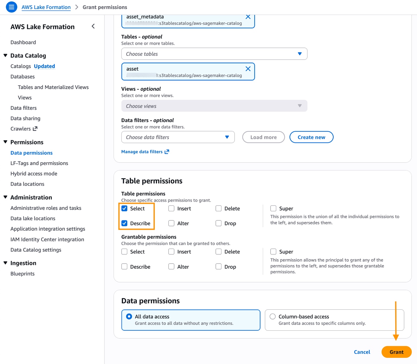
Figure 2 – Grant access to Amazon SageMaker Catalog resources
When choosing the catalog in the Lake Formation console, you must choose the full S3 Tables catalog identifier (ACCOUNT_ID:s3tablescatalog/aws-sagemaker-catalog) to see the asset_metadata database.
Access S3 Tables data by creating a Quick Sight dataset using an Amazon Athena data source and the custom SQL option. An S3 Tables data source is also available but requires additional permissions. See Introducing new data source with S3 Tables in Amazon Quick for using S3 Tables as an Amazon Quick data source.
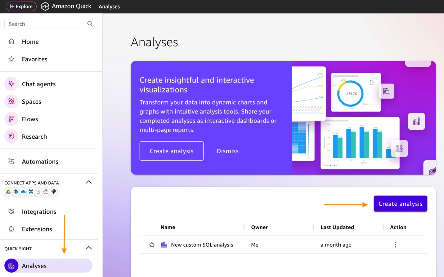
Figure 3 – Create Amazon Quick Sight analysis

Figure 4 – Create dataset
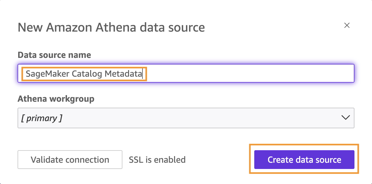
Figure 5 – Create data source
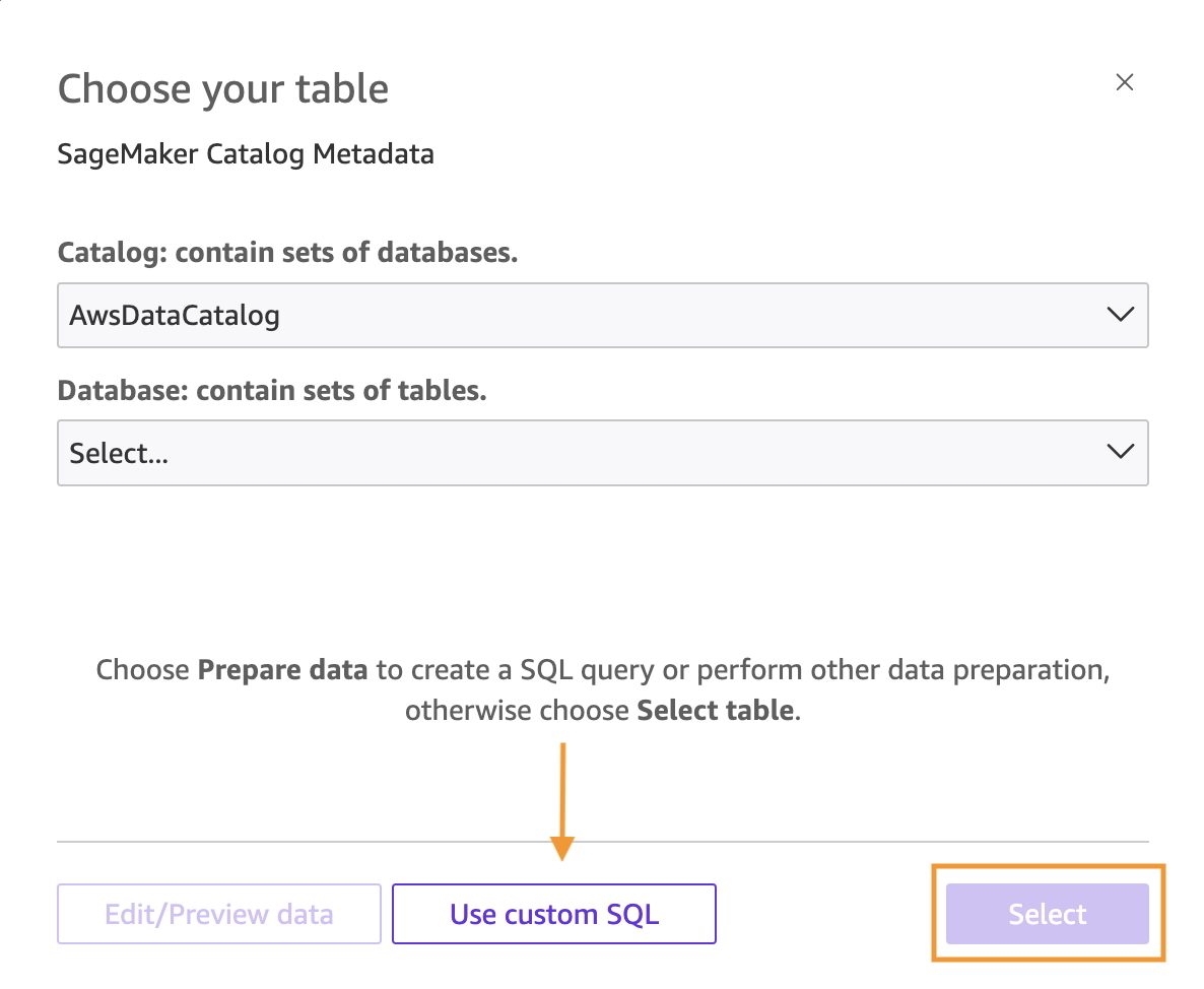
Figure 6 – Use custom SQL
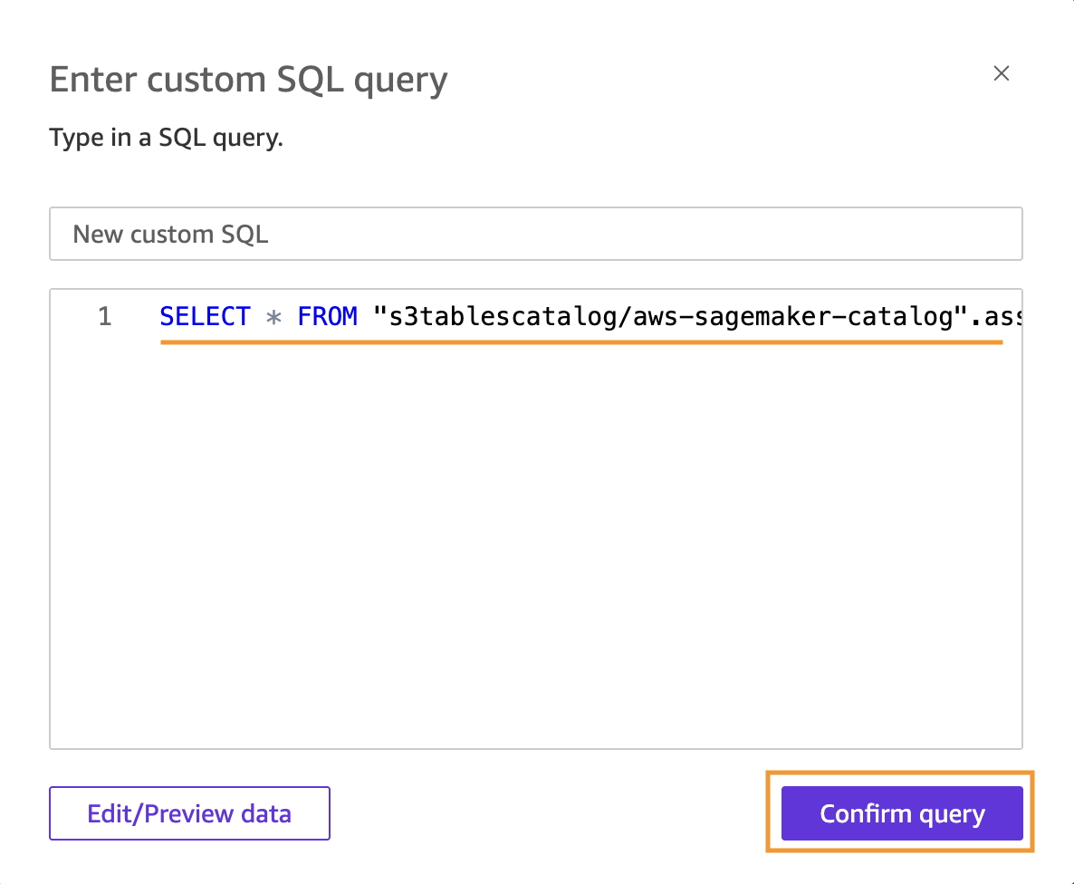
Figure 7 – Enter custom SQL
SELECT * FROM "s3tablescatalog/aws-sagemaker-catalog".asset_metadata.asset
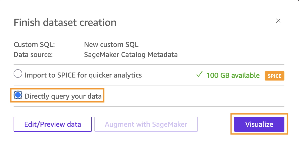
Figure 8 – Directly query your data
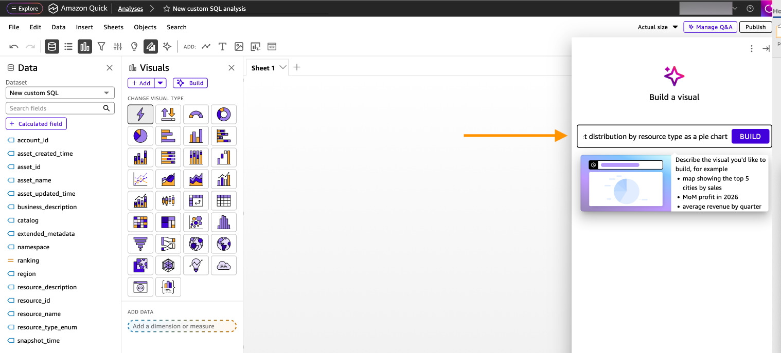
With Amazon Quick, you can build governance dashboards using natural language prompts. This removes the need for manual field configuration. This approach is faster and more intuitive than traditional dashboard building.The Amazon Quick Sight user must have AdminPro or AuthorPro subscription (the Build feature isn’t available for Reader users).Start building your dashboard with the following steps:
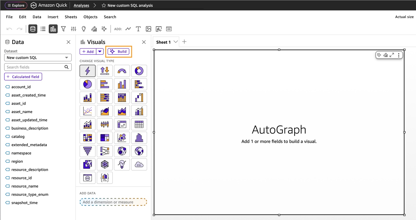
Figure 9 – Amazon Quick build dashboard
Create each visualization using natural language. For each of the six recommended visualizations, enter the corresponding natural language prompt, select Build, then choose ADD TO ANALYSIS.
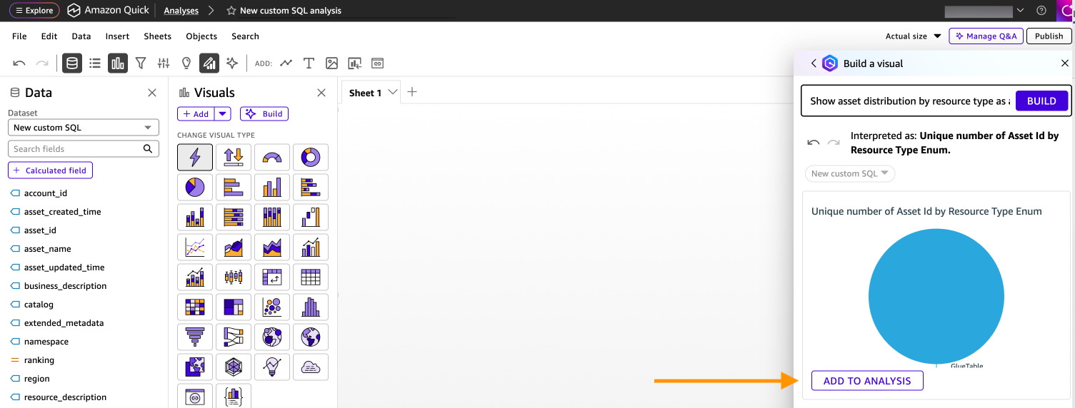
Figure 11 – Add to analysis
Visualization 1: Asset inventory by type
Show count of asset_id by resource_type_enum as a pie chart
After the pie chart is created, choose ADD TO ANALYSIS.
Visualization 2: Documentation completeness
Show count of asset_id where business_description is not null asa KPI
After the KPI is created, choose ADD TO ANALYSIS.
Visualization 3: Monthly registration trends
Show count of asset_id by asset_created_time month as a line chart
After the line chart is created, choose ADD TO ANALYSIS.
Visualization 4: Asset count by account
Show count of asset_id by account_id as a bar chart
After the bar chart is created, choose ADD TO ANALYSIS.
Visualization 5: Namespace distribution
Show count of asset_id by namespace as a treemap
After the treemap is created, choose ADD TO ANALYSIS.
Visualization 6: Resource type by namespace
Show count of asset_id by resource_type_enum and namespace as a heat map
Choose ADD TO ANALYSIS
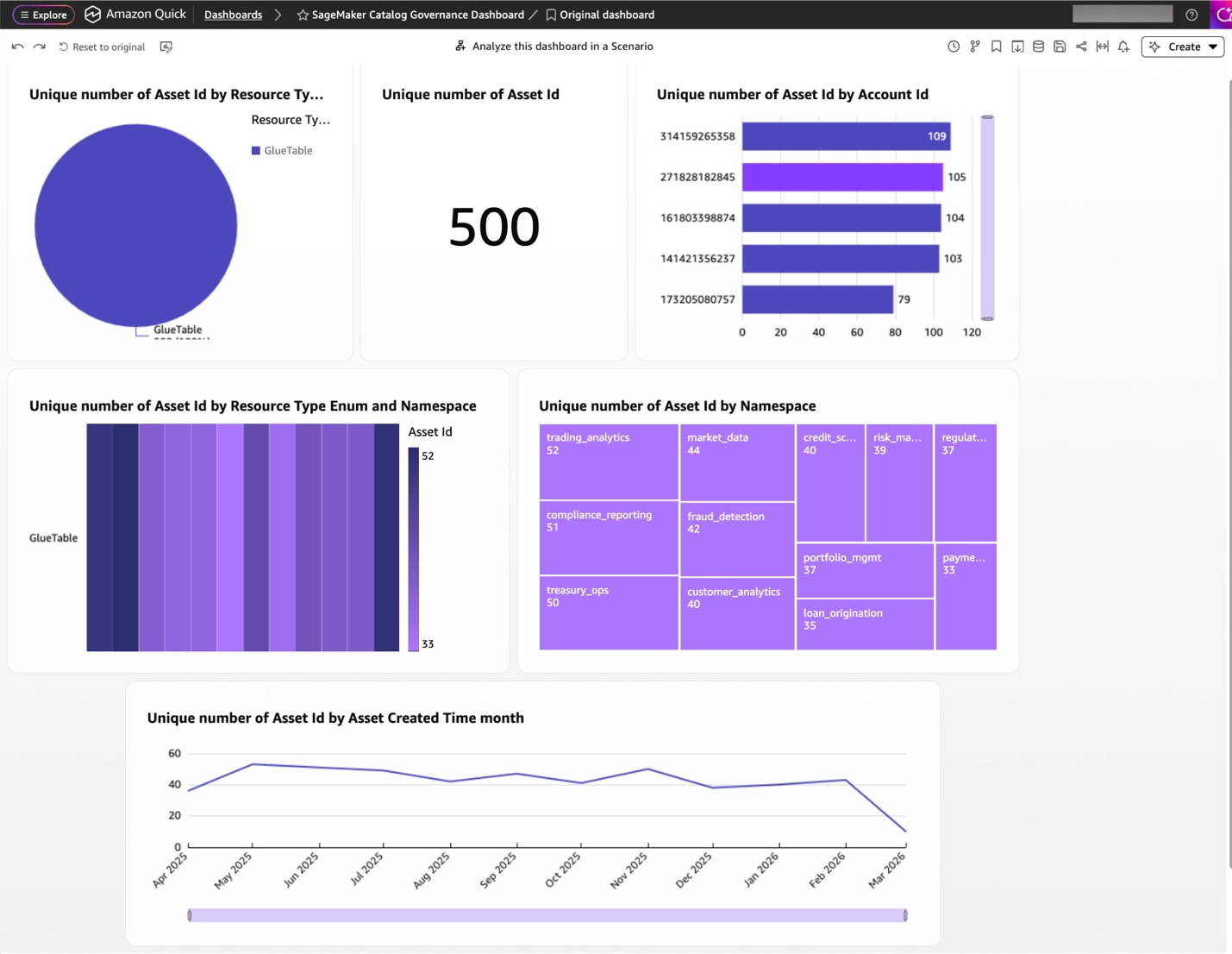
Figure 12 – Amazon SageMaker Catalog governance dashboard
After you publish, you can ask questions about your governance data:
Amazon Quick analyzes your data and provides insights with supporting visualizations.
Create automated governance reports for data stewards and compliance teams:
Amazon Quick will automatically generate a summary with key governance insights, including Total asset counts and growth trends, Documentation completeness metrics, Ownership coverage statistics, and Classification distribution analysis.
Build governance reports that combine multiple dashboards:
Amazon Quick will generate a narrative report combining your visualizations with AI-generated insights. Share the reports with leadership or compliance teams.
Governance dashboards contain metadata such as ownership and classification details. Restrict access to users who need it. In the Amazon Quick Sight console, open the dashboard, choose Share, and grant access to named users or a dedicated Quick Sight group (for example, data-stewards) instead of selecting Everyone in this account. Review the dashboard’s permissions periodically and remove entries that are no longer needed.
To avoid ongoing charges, clean up the resources created in this walkthrough. Delete Amazon Quick Sight resources including the dashboard, analyses, and dataset.
In this post, you connected Amazon Quick Sight to your Amazon SageMaker Catalog metadata export, built governance dashboards using the Amazon Quick natural language prompts. This approach gives data stewards and compliance teams visibility into catalog health through six key visualizations covering asset inventory, documentation completeness, registration trends, account distribution, classification coverage, and stale asset detection.
Together with the metadata export and SQL query capabilities covered in the Analyzing your data catalog: Query SageMaker Catalog metadata with SQL post, this solution provides a complete, low-overhead governance monitoring pipeline from raw catalog metadata to executive-ready.
To learn more about Amazon SageMaker Catalogs, see Amazon SageMaker Catalog documentation. To expand the work done with Amazon Quick, review Amazon Quick Sight documentation.
Post Syndicated from Jason Ramos original https://aws.amazon.com/blogs/big-data/accelerate-sql-development-with-sagemaker-data-agent-in-query-editor/
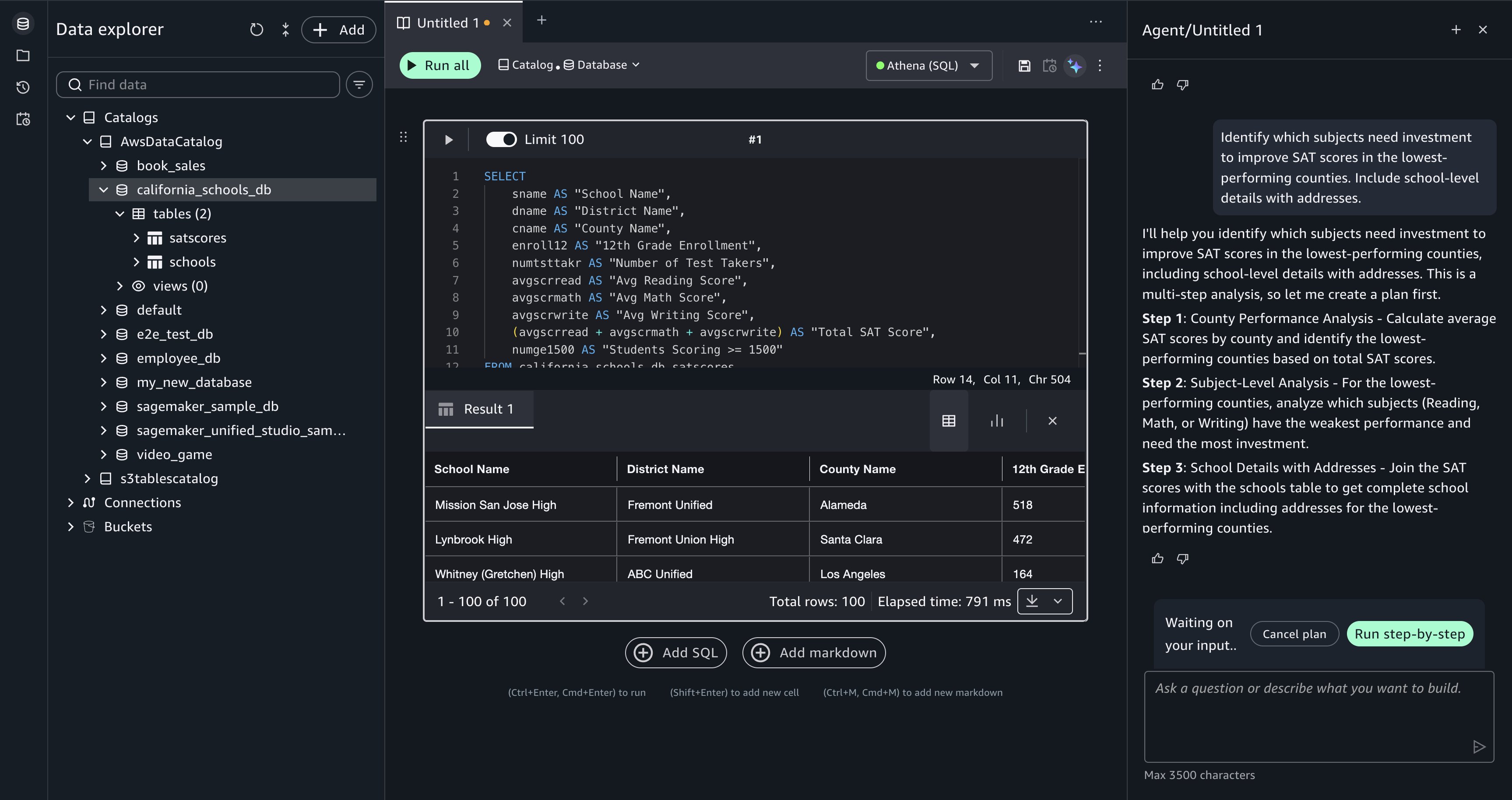
When you develop SQL against Amazon Redshift and Amazon Athena, you spend time finding the right tables across hundreds of databases, writing complex joins and aggregations, debugging failed queries without context from previous attempts, and re-specifying filters for every new question. Amazon SageMaker Data Agent in Query Editor takes a different approach. You describe what you need in natural language, and the Data Agent generates the SQL. It references your actual tables through AWS Glue Data Catalog, proposes step-by-step plans for complex questions, retains context across your session, and offers one-click error recovery with Fix with AI. In this post, you learn how to use Data Agent in Query Editor to explore data, build multi-step analyses, recover from errors, and summarize results using a public education dataset.
You can go from a natural language question to executable SQL in seconds. Data Agent in Query Editor provides a conversational interface with direct access to your AWS data environment, so you spend less time on query mechanics and more time on analysis. Data Agent in Query Editor focuses specifically on SQL development against Amazon Redshift and Amazon Athena. (For Python, SQL, and PySpark across broader analytical and machine learning (ML) workloads, use Data Agent in notebooks.)
Data Agent provides four key capabilities:
Data Agent integrates with AWS Glue Data Catalog and reads your actual table names, column types, descriptions, and relationships, so generated SQL references your real tables. Each follow-up question builds on your current Query Editor session—the SQL cells in your querybook, the active connection, your selected cell, and execution results from previously run cells. For complex requests, Data Agent produces a structured plan that specifies which data to retrieve, how to aggregate it, and what filters to apply. You review and approve each step before Data Agent proceeds. When a query fails, choose Fix with AI to get a corrected query based on the error and the failed cell’s context.
[Figure 1: The Query Editor Fix with AI panel, showing a corrected SQL query ready for your review.]
In this section, you use Data Agent in Query Editor to analyze California schools data and identify where SAT improvement investment has the most impact. The walkthrough covers four tasks:
The same workflow applies to your own data, whether you are analyzing sales figures, operational metrics, or financial records.
The California schools dataset contains SAT score results, school demographic information, and county-level data for public schools across California. The dataset includes tables that organize SAT scores by subject (reading, writing, math), school details (name, address, county, district), and enrollment figures. After you upload the data into your project database, you directly access the tables from Query Editor through your Amazon Athena or Amazon Redshift Lakehouse connection.
To complete this walkthrough, you need intermediate SQL knowledge and basic familiarity with the AWS Management Console. You don’t need prior AWS Glue experience, but familiarity with data catalogs (centralized metadata repositories) helps.
You can choose one of two setup paths:
sagemaker_sample_db) with pre-loaded data. To explore it, choose Data in the navigation pane, expand AwsDataCatalog, and select sagemaker_sample_db.Running queries against Amazon Athena or Amazon Redshift might incur costs. For pricing details, refer to Amazon Athena pricing and Amazon Redshift pricing. For detailed setup instructions, refer to AWS Identity and Access Management (IAM)-based domains and projects. Before starting the walkthrough, you must have a SageMaker Unified Studio IAM-based domain with a project using the SQL analytics or All Capabilities project profile. The project automatically provisions an AWS Glue database, the required IAM role, and Athena or Redshift Lakehouse connections.
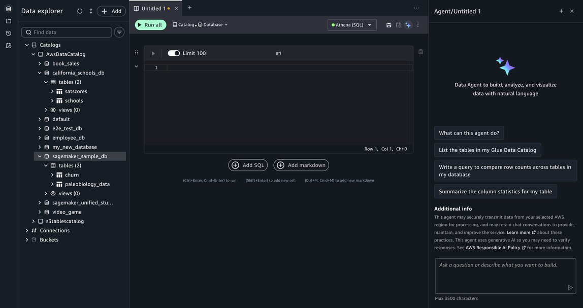
[Figure 2: The Data Explorer panel in Query Editor, showing the california_schools_db and sagemaker_sample_db tables.]
Explore available data. To start, enter the following prompt in the Data Agent panel:
Data Agent searches AWS Glue Data Catalog, locates the relevant tables, and generates an initial exploratory query that retrieves SAT score records. It adds a SQL cell directly to your querybook.
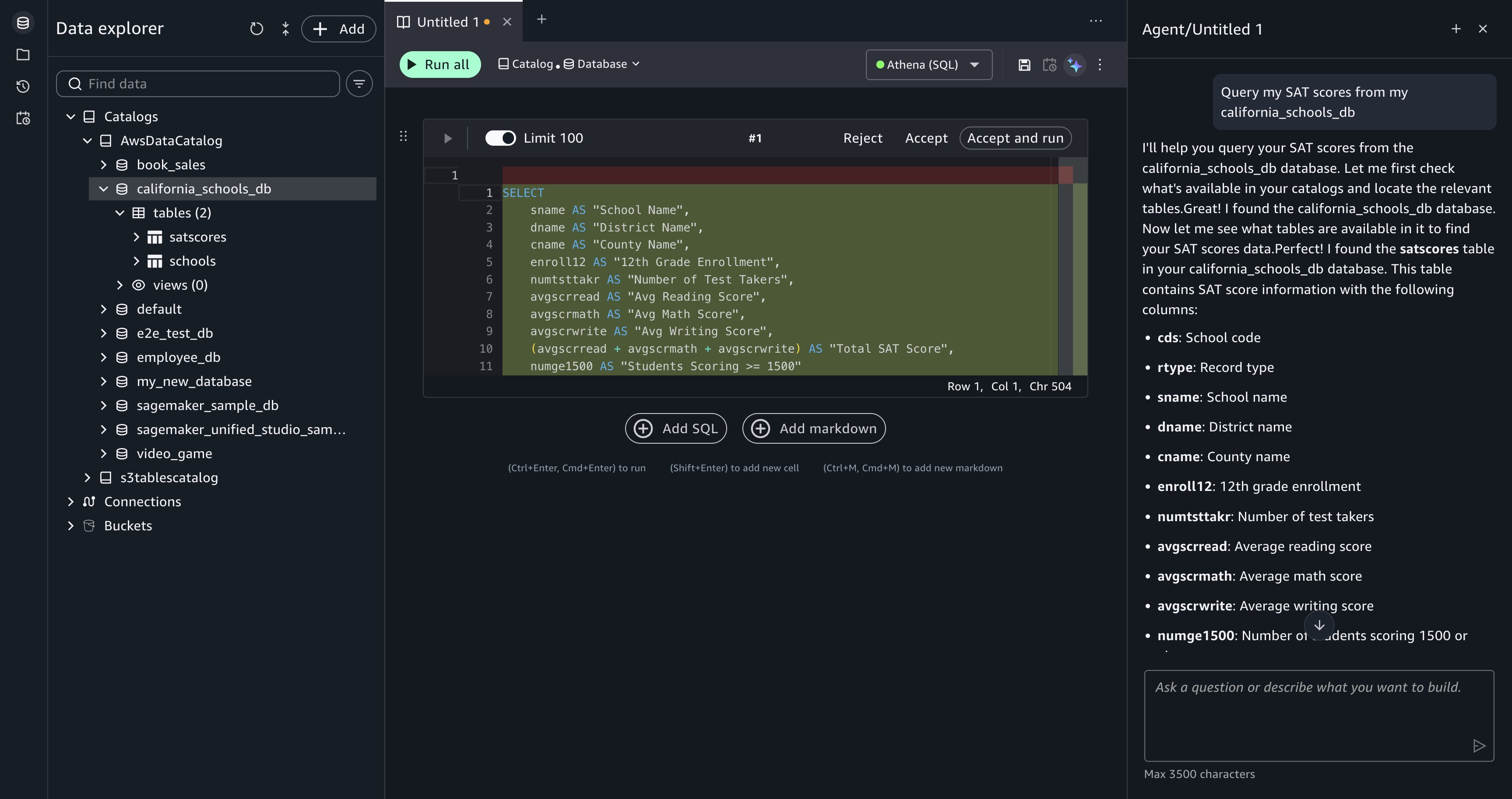
[Figure 3: Data Agent returns an exploratory query for the california_schools_db tables, ready for your review.]
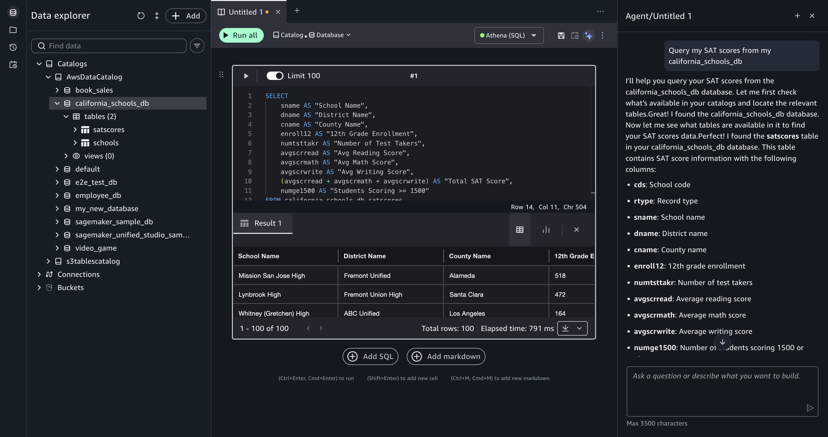
[Figure 4: The SQL query results appear beneath the cell after you choose Accept and run.]
Build a multi-step analysis plan. With the data explored, enter a more complex analytical question:
Data Agent proposes a step-by-step plan before generating SQL. For this request, Data Agent breaks the question into three steps:
Review the plan in the Data Agent panel and choose Run step-by-step to proceed.
[Figure 5: Data Agent proposes a multi-step plan with options to Cancel plan or Run step-by-step.]
Data Agent generates SQL for each step and adds it as a separate querybook cell. Review each cell’s SQL in the comparison view, then choose Accept and run to execute it. The results from each step are visible inline, so you can verify the intermediate output (county-level aggregations, the filtered ranking, and the final school list) before moving to the next step. When the steps are complete, your querybook contains the full analytical progression from raw scores to a detailed investment list.
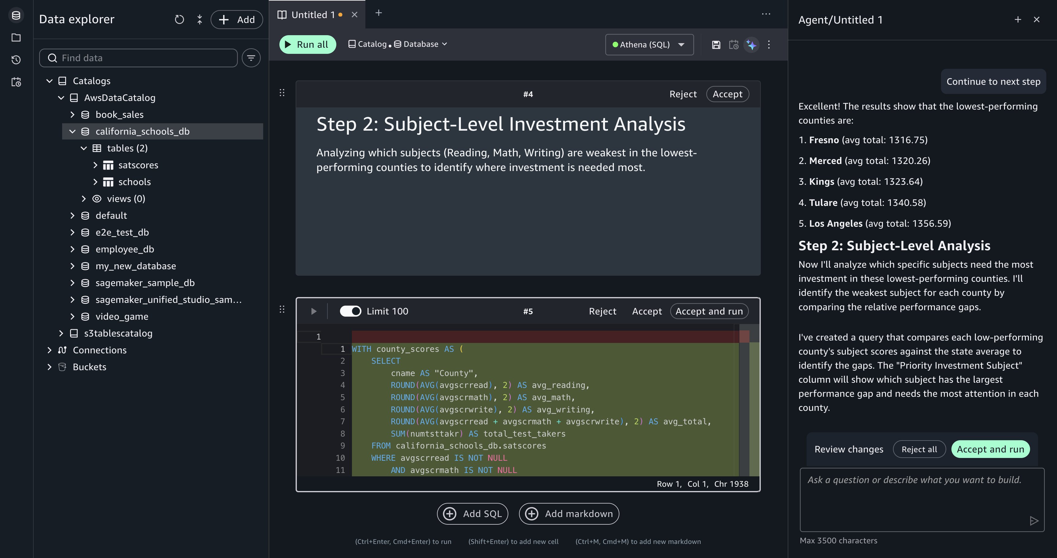
[Figure 6: Each plan step produces a querybook cell that you can review and run independently.]
Summarize insights from your queries. After running the analysis, enter the following prompt:
Data Agent has context on your querybook, including the SQL and the query results from each cell. It generates a natural language summary: which counties are underperforming, which subjects (reading, writing, or math) need the most attention in each county, and how many schools appear on the investment list. This summary provides a starting point for a report or presentation.
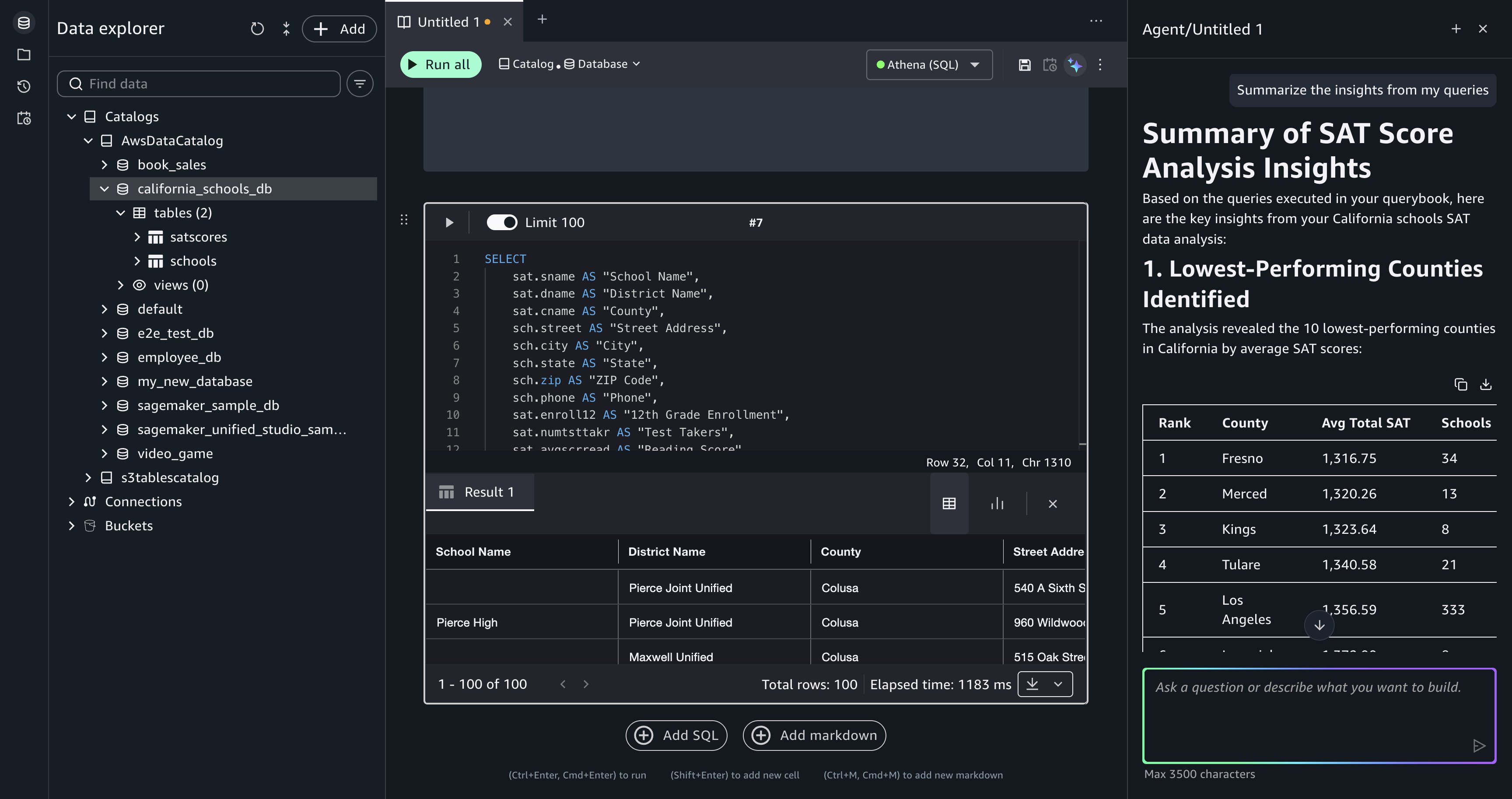
[Figure 7: Data Agent summarizes insights from the accumulated query results in the querybook.]
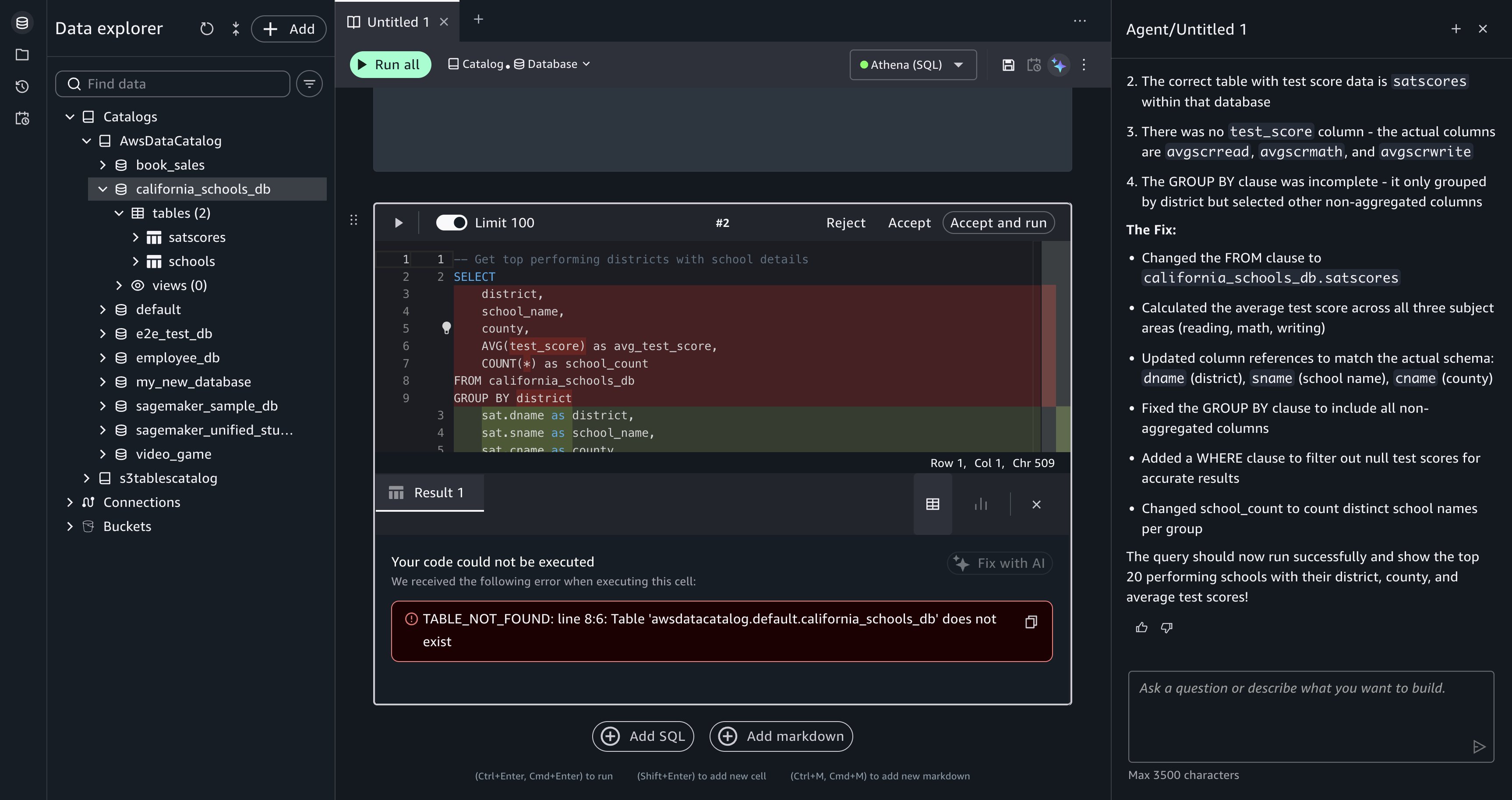
Recover from a failed query. During the analysis, a generated query might produce an error, for example, referencing a column name that doesn’t match the schema or a join condition that returns unexpected results. When a cell fails, Query Editor displays the error message and a Fix with AI option.
Choose Fix with AI, and Data Agent reads the error in the context of the failed cell, then generates corrected SQL and updates the querybook cell. Run the corrected cell to verify the fix.
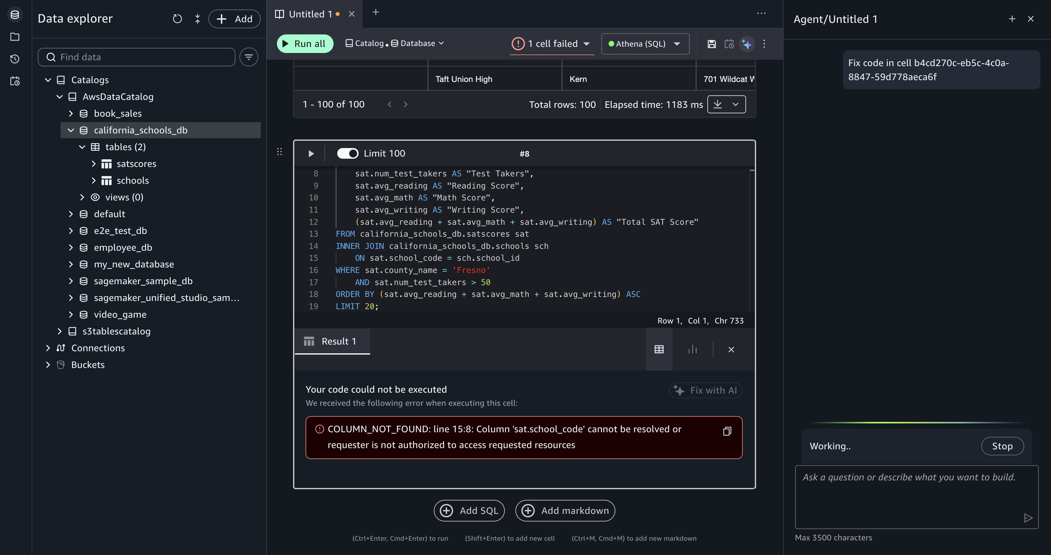
[Figure 8: After you choose Fix with AI, Data Agent is prompted to generate a corrected query for the failed cell.]
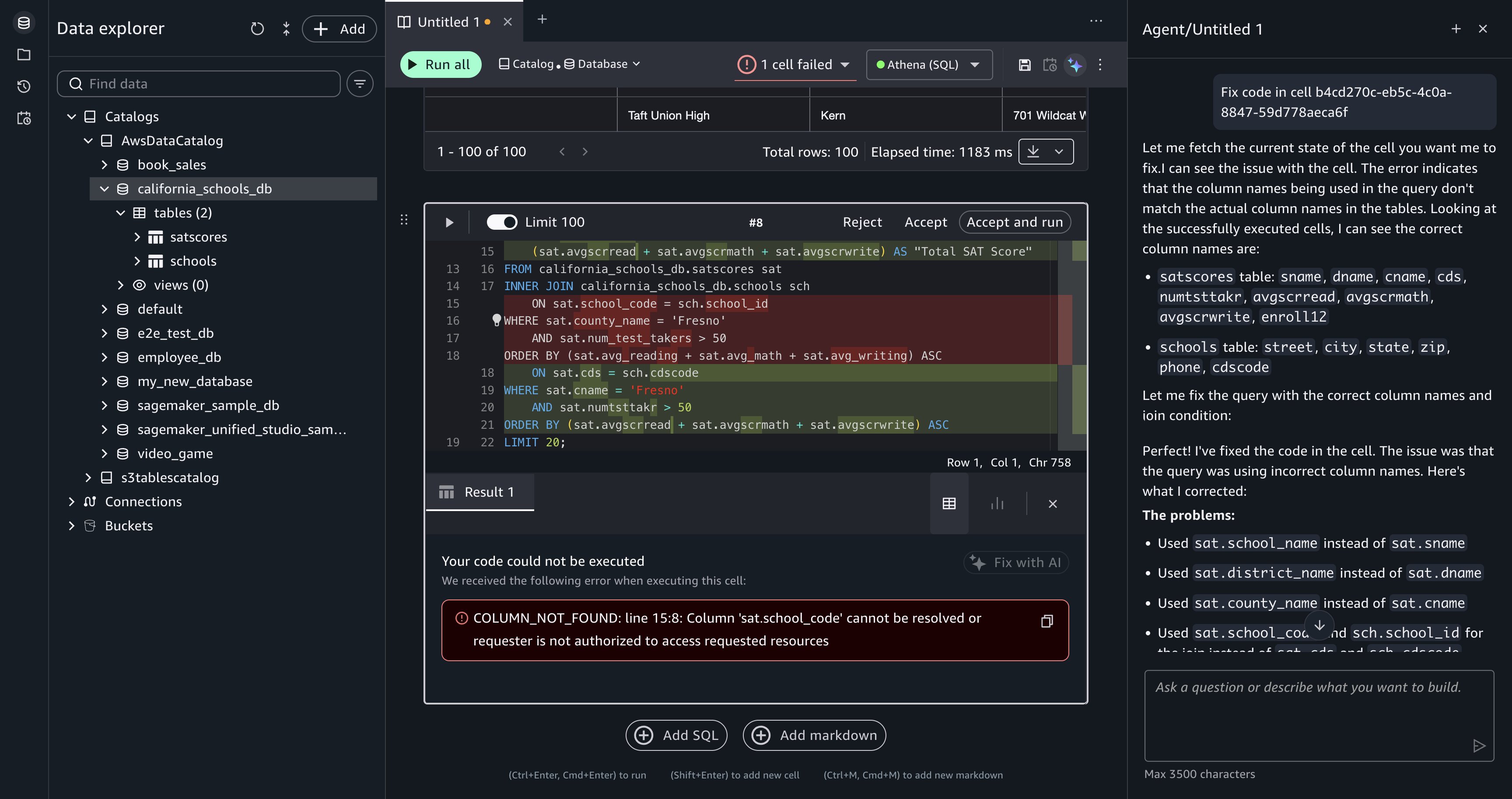
[Figure 9: Data Agent returns corrected SQL for you to review.]
Data Agent operates within your AWS environment and only accesses data that your IAM policies explicitly permit. Your existing IAM access controls and AWS Lake Formation permissions determine what data Data Agent can reach. To use Data Agent, your project role must have permissions to invoke specific Amazon DataZone APIs. For more information, refer to Actions, resources, and condition keys for Amazon DataZone.
Data Agent includes content filtering that prevents it from responding to off-topic requests, requests to reveal its system prompt, and requests for internal technical implementation details. Data Agent is restricted to AWS-related topics and English-language output.
Amazon SageMaker stores your natural language prompts and generated SQL in the AWS Region where you created your SageMaker Unified Studio domain. Data Agent doesn’t store your data, querybook context, or catalog metadata.
To opt out of data usage for service improvement, configure an AI services opt-out policy for Amazon DataZone in AWS Organizations. For more information, refer to Data storage in the SageMaker Data Agent, Service improvement, and AI services opt-out policies.
The walkthrough creates querybook cells in your Query Editor session but doesn’t provision standalone infrastructure. To remove the generated SQL cells, delete them from your querybook or delete the querybook itself.
If you uploaded the California schools dataset specifically for this walkthrough, remove the following resources to avoid ongoing charges:
Data Agent in Query Editor brings conversational, catalog-aware SQL development to your Amazon Redshift and Amazon Athena workloads. In this post, you explored unfamiliar data, built a multi-step investment analysis, recovered from query errors, and summarized findings through natural language prompts.
Data Agent works within your existing IAM and AWS Lake Formation security controls, keeps your data within your AWS environment, and retains context across your analytical workflow so each question builds on the last.
Get started with these next steps:
Show me the top 10 tables in my catalog with the most columns. For setup, refer to the SageMaker Unified Studio getting started guide.Which product categories had declining revenue quarter-over-quarter, and which regions drove the decline? and review Data Agent’s plan step by step.For more information, refer to the Amazon SageMaker Data Agent documentation, the What’s New blog post, Amazon Redshift documentation, and Amazon Athena documentation. To learn how Data Agent works in notebooks, refer to Accelerate context-aware data analysis and ML workflows with Amazon SageMaker Data Agent.
Post Syndicated from Ryan Smith original https://www.servethehome.com/microsoft-to-join-the-ai-dev-mini-pc-market-with-upcoming-surface-rtx-spark-dev-box/
Microsoft is joining the AI dev box mini-PC market with the announcement of the Surface RTX Spark Dev Box. Due later this year, it will offer a pre-loaded dev environment, powered by NVIDIA’s new RTX Spark SoC
The post Microsoft to Join the AI Dev Mini-PC Market With Upcoming Surface RTX Spark Dev Box appeared first on ServeTheHome.
Post Syndicated from Crosstalk Solutions original https://www.youtube.com/shorts/excZRXQEZMg
Post Syndicated from jzb original https://lwn.net/Articles/1076377/
The EFF has a blog
post looking at a new bill in California that would exempt
open-source operating systems from the Digital Age Assurance Act
passed last year, but has problems of its own:
While the open source exemption, if passed, would improve the law, the
remaining amendments proposed by AB 1856 would require all web
browsers and websites to request and collect users’ ages. This is an
expansion of last year’s AB 1043’s age-bracketing system that
compounds its constitutional harms to users’ speech, privacy, and
security.[…] EFF understands this amendment to exempt open-source
operating systems from the requirement to collect and transmit users’
age-bracket data. That is a definite win for open-source
developers. The bill is narrower now than it was before, and lawmakers
clearly responded to concerns raised by EFF and the broader
open-source community.Some important questions still remain—for example, it is unclear
how the law would apply when an open-source operating system is
incorporated into a commercial product or service. And, given the
structure of where the exemption is placed under the “operating system
provider” definition, lawmakers could stand to clarify that the
exemption applies to open-source operating systems and
applications.
LWN covered
California’s age-attestation law in March.
Post Syndicated from David Higgs original https://www.rapid7.com/blog/post/dr-swiss-cheese-model-helps-choose-mdr-providers
Not all managed detection and response (MDR) solutions are equal. Finding the differences between vendors can be quite hard, and then understanding how those differences impact your business can be even harder. For instance, you may come across an MDR provider whose pricing is based on how much data you ingest rather than the number of assets you protect.
Ingestion-based solutions have the potential to be more cost effective if you’re selective about what security telemetry you ingest – but then who analyzes the impact of the logs you’re leaving out until they’re needed?
Or, consider an MDR solution that’s more EDR with just a few additional log sources. For some organizations this is a perfectly optimal fit. But, how often are logging blind spots reviewed and accepted as a risk? In my experience, very rarely.
I like to spend time educating customers on the importance of defense in depth, and partners on how to clearly demonstrate its importance when it comes to catching and stopping attacks.
One of my favorite ways of explaining defense in depth is the “Swiss Cheese model.”

⠀
It’s a risk model successfully used across industries like aviation safety, engineering and other domains. Its guiding principle is that a single safeguard is not fool-proof when it comes to mitigating accidents, and that true resilience is dependent upon multiple layers of monitoring and control.
The great thing about this model is that it translates really well when it comes to security operations and the technologies (SIEM) and services (MDR) that underpin it. In the case of these solutions, each slice of “cheese” is a combination of log source and detection rules across multiple attack surface domains – think endpoint, identity, cloud, or network – each reinforced by multiple log sources and detection rules that ladder up to those domains.
The detection rules that help us spot attackers’ actions are the other half of the “cheese layer.”
The logs and detection rules working in combination is what represents the whole slice of cheese.
For example, let’s say you have an agent capturing activity on all of your servers and endpoints. But, an attacker has managed to steal some VPN credentials to log in to your corporate environment like a normal user. There is no agent on the attacker’s machine, only on corporate users’ machines.
Their next step is to enumerate the environment, which can be a combination of passive monitoring and active scanning. Their task? Finding that next stepping stone so they can ultimately make their way to gaining domain admin credentials or exfiltrating data from the environment as an example.
There are lots of activities the attacker can implement to achieve this without alerting any agents.. But, what if we have some log sources monitoring active directory, firewall/VPN access, and even a network-based sensor monitoring traffic going in and out of the firewall? It means we can gain additional visibility, capturing this malicious activity before it escalates.
Other methods of initial access – like phishing – can also be captured through adding log sources for email solutions and any other email-related activities. An example could be changing email inbox rules so that an unsuspecting user can’t see all the replies to the emails the attacker is sending from their mailbox.
Not every log source is able to capture every malicious activity from an attacker, which is why we need multiple layers. The holes can be for a few reasons – visibility gaps in the log source e.g. if you only have your EDR installed on 90% of the assets that can have it installed there is a clear hole. There are also detection rule shortfalls – either a rule does not exist to alert on that activity when it occurs or perhaps the log source is limited in how it records the behavior which makes creating a detection not possible.
This the whole foundational principle of Swiss cheese theory, that we should expect an attacker to be able to circumvent a single layer
For each type of asset in your environment, it’s a great idea to draw up a Threat Model. For the purposes of this blog, the below model is fairly high level. An organization-specific threat model should go more in depth, but hopefully you can get the general idea.
Think about how an attacker might attempt to use these assets either to monetize the environment (i.e. ransomware) or as a stepping stone to a more critical asset.
Think about the log sources that would contribute towards highlighting attacker activity on those assets. For instance:
Windows and Mac workstations
EDR agent
Email logs
VPN/firewall authentication logs
Single sign on (SSO) logs
Domain controller
Lightweight directory access protocol (LDAP) and Active Directory logs
EDR agent
Network sensor
As I stated, this is high-level and not exhaustive, but the idea is to think of the attacker’s actions and all of the potential log sources that could detect those actions in order to ensure you’re able to capture this activity.
Of course, this model might come under scrutiny when looking at the costs of ingesting and storing log data. Organizations then have to balance the cost of technical detections with the value they provide. In real terms, if you must choose three out of five log sources because that’s what you can afford, you should pick the three most valuable to your business.
The value should come from a combination of the number of detections they drive and the quality of those detections. For example, one log source might drive 1,000 detection types, but the detections themselves have a high benign positive ratio (say 29 in 30 are benign) on 80% of the detections, whilst another log source might drive 500 detections but have a much lower benign positive ratio of 1 in 10. This forces detection engineers to create the most optimal log-and-detection rule sets in order to optimize the cost of the SIEM.
All those calculations above sound complex, right? Much of that complexity can be made simpler with an asset-based pricing model, such as the one used by Rapid7.
The price is fixed on the number of servers and workstations, and customers can connect any number of log sources. This means when you’re modeling threats and detection of those threats, there are no cost constraints to consider for onboarding additional log sources, which would improve detection fidelity.
With that in mind, here’s a few questions I would suggest customers ask themselves to establish which solution is the right one for them:
Size: How big are you in terms of employees or number of assets?
A 5,000 employee business with a 20 person Security team is more likely to need a SIEM with unlimited ingestion than a 20 person business with one combined IT/security person.
Assets and tech stack: What types of assets are being protected and what technologies are in use?
This helps dictate whether an EDR with a few extra log sources is more suitable as the backbone of an MDR service versus One that incorporates a wide variety of telemetry sources.
Whilst the lines aren’t clear cut, these can be general areas to investigate and better understand. Other factors that also come into play are things like the type of threat actors that might target your organization. Here is an example of what it could look like worked into a threat model I spoke about.
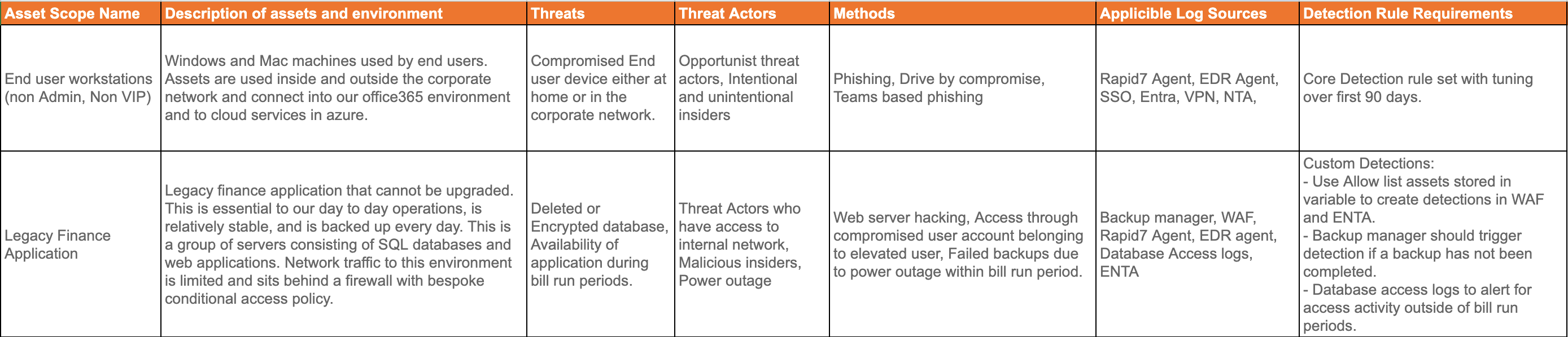
Attempting to compare asset-based and ingestion-based solutions can be tricky. If you try to constrain to a consistent set of log sources for the two solution types, you could be depriving your organization of the main benefit of an asset-based pricing structure: the ability to bring more log sources and detections – and therefore additional layers of protection – for the same cost. This would, of course, give you a lower cost-per-detection. Let’s take a look at some ideas that might help:
Look at cost-per-detection when fixing a cost limit.
Evaluate quality of detections within the model environment using the cost model constraint.
Detection noise under normal conditions.
Give detection rules a score:
|
MDR / SIEM Solution 1 |
MDR / SIEM Solution 2 |
||
|
Metric 1 – Solution Coverage |
|||
|
Cost |
$100,000.00 |
$100,000.00 |
|
|
Total Applicable log sources for example customer |
30 |
20 |
|
|
Points |
30 |
30 |
0 |
|
Metric 1.5 – Solution Detection Value |
|||
|
Cost |
$100,000.00 |
$100,000.00 |
|
|
Total detection rules applicable to log sources |
10,000 |
7,000 |
|
|
Cost per Detection |
$10.00 |
$14.29 |
|
|
Points |
30 |
30 |
0 |
|
Metric 2 – Quality 1 – Offensive Testing in isolated environment |
|||
|
Total tests conducted by offensive team |
18 |
18 |
|
|
Total detections triggered per solution |
15 |
16 |
|
|
% of coverage |
83% |
89% |
|
|
Points |
30 |
0 |
30 |
|
Metric 3 – Quality 2 – rules triggered by normal user activity |
|||
|
Total investigations triggered in 30 days |
100 |
130 |
|
|
Total True Positive investigations in 30 days |
90 |
87 |
|
|
True Positive Ratio % |
90% |
67% |
|
|
Points |
40 |
40 |
0 |
|
Metric 4 – Monthly SOC operations overhead – tuning and detection rule writing (N/A for Managed) |
|||
|
Hourly rate |
$200 |
$200 |
|
|
Tuning time in hours over the last 30 days |
10 |
12 |
|
|
Detection rule writing time in hours over the last 30 days |
6 |
8 |
|
|
Monthly soc operations overhead in $ |
$3,200.00 |
$4,000.00 |
|
|
Points |
10 |
10 |
0 |
|
Metric 5 – Implementation time |
|||
|
Hourly rate |
$200 |
$200 |
|
|
Time to implement solution in hours for example customer |
40 |
40 |
|
|
Total PS cost for solution implementation |
$8,000.00 |
$8,000.00 |
|
|
Points |
10 |
0 |
0 |
|
Total Points |
110 |
30 |
|
⠀
Whilst there are no absolutes, there are some good rules that can help you on the path to choosing an MDR provider that works best with and for your organization. Focusing on the assets and technologies that you want to protect, and looking at log sources and detections that support that is a great place to start.
The higher the importance and complexity of the asset, the more layers you ideally want, and having the table above to clearly define your quality metrics will help you consider whether a solution is the right fit for you in terms of technology, service, and economics.